The effectiveness of solar radiation management using fine sea spray across multiple climatic regions

Marine cloud brightening (MCB) geoengineering aims to inject aerosols over oceans to brighten clouds and reflect more sunlight in order to offset the impacts of global warming or to achieve localized climate cooling. The relative contributions of direct and indirect effects in MCB implementations remain uncertain. Here, we quantify both effects by designing model simulations to simulate MCB for five open-ocean regions around the globe. Our results show that a uniform injection strategy that does not depend on wind speed captured the sensitive areas of the regions that produced the largest radiative perturbations during the implementation of MCB. When the injection amounts are low, the sea salt aerosol effect on shortwave radiation is dominated by the indirect effect via brightening clouds, showing obvious spatial heterogeneity. As the indirect effect of aerosols saturates with increasing injection rates, the direct effect increases linearly and exceeds the indirect effects, producing a consistent increase in the spatial distributions of top-of-atmosphere upward shortwave radiation. This study provides quantifiable radiation and cloud variability data for multiple regional MCB implementations and suggests that injection strategies can be optimized by adjusting injection amounts and selecting areas sensitive to injections.

1 Introduction

As global temperatures continue to rise, the international community is facing an unprecedented challenge to achieving the ambitious goal set in the Paris Agreement of limiting global warming to within 1.5 °C (Mengel et al., 2018). One of the key outcomes of the recently concluded 28th Conference of the Parties (COP28) was the completion of the first Global Stocktake (GST), a midterm assessment of the progress made by countries towards achieving the climate goals of the Paris Agreement. However, the report highlighted that current efforts to reduce emissions have fallen short of the intended targets (https://unfccc.int/documents/636608, last access: 25 February 2025). Against this backdrop, scientists are turning their attention to geoengineering methods that reduce or offset the impacts of climate change through artificial interventions in the climate (Visioni et al., 2023). Some geoengineering methods seek to capture or remove CO₂ from the atmosphere in order to increase carbon sinks, while others focus on modifying solar radiation, reducing incoming solar shortwave radiation, or reflecting more sunlight to cool Earth, which is known as solar radiation management (SRM) (Lenton and Vaughan, 2009). Of these methods, marine cloud brightening (MCB) has a realistic basis and is considered the most feasible SRM method for regional applications (Latham et al., 2014). It has been observed that exhaust emissions from ocean-going vessels can lead to brighter clouds, with clear ship tracks also visible from satellites, and MCB aims to replicate this effect by spraying sea salt aerosols (Chen et al., 2012).

Aerosol–cloud interactions and their impacts on climate are complex (Rosenfeld et al., 2014, 2019). Injected sea salt aerosols affect clouds through indirect effects (Paulot et al., 2020). In the case of a constant liquid water content, an increase in cloud droplet number concentration (CDNC) decreases the cloud droplet size and increases the total surface area of cloud droplets, thereby enhancing the cloud albedo, forming brighter clouds, and reflecting more sunlight back into space (the first indirect effect or Twomey effect) (Twomey, 1974). At the same time, the decrease in cloud droplet size suppresses precipitation, thereby increasing a cloud's lifespan and optical thickness (the second indirect effect of aerosols) (Albrecht, 1989). In addition, those aerosols that are not injected into the clouds scatter more sunlight back into space through the direct scattering effect (Ahlm et al., 2017; Partanen et al., 2012; Zhao et al., 2021). Therefore, this method is also called marine sky brightening (MSB), which can work even when there are no clouds. Here, we collectively refer to the practice of injecting sea salt aerosols as MCB.

Compared to other geoengineering schemes, such as stratospheric aerosol injection (SAI), MCB has unique advantages. For example, the sprayed aerosols have lower environmental risks and can be applied locally to change the regional climate (Latham et al., 2008). Their deployment costs are relatively low and flexible (Kravitz et al., 2014; Latham et al., 2012, 2014). However, despite these potential advantages, the long-term effects and potential risks of MCB are not fully understood, and there are significant uncertainties as well as ethical, political, and environmental risks (Carlisle et al., 2020; Feingold et al., 2024). Therefore, most of the current literature examines the environmental and climate impacts of MCB implementation through modeling.

Table S1 in the Supplement summarizes the results of current modeling simulations of MCB with sea salt aerosols, together with their implementation strategies. Most MCB studies use Earth system models to assess the impacts of the implementation of MCB on climate. Early MCB studies assumed the effects of MCB implementation by setting a fixed CDNC or directly modifying the cloud effective radius (r_e), ignoring processes such as generation, transport, dry and wet deposition, and activation of injected sea salt aerosols and not including the direct radiative effect of aerosols. With the development of models, researchers started to conduct more detailed studies by injecting aerosols or increasing sea salt aerosol emissions, taking into account the post-injection processes of aerosols mentioned above.

The implementation region of MCB is crucial. Existing studies have focused on the impacts of MCB implementation in three key areas: open oceans globally, the equatorial region (between 30° S and 30° N), and coastal areas with widespread marine stratocumulus clouds. Alterskjær et al. (2012) used the cloud-weighted susceptibility function to find the regions most sensitive to the injection of sea salt aerosols. Similarly, Jones and Haywood (2012), using an iterative method, determined the 10 % of the marine regions that are globally most suitable for implementing MCB. The contributions of direct and indirect effects of aerosols during the implementation of MCB are still uncertain, and quantitative assessment of both is lacking (Haywood et al., 2023; Partanen et al., 2012).

Here, we use the two-way coupled Weather Research and Forecasting–Community Multi-scale Air Quality (WRF–CMAQ) model, combined with previous studies on the region and injection strategies, to implement MCB in five open-ocean regions. This study simulates the regional radiation and cloud responses caused by injecting sea salt aerosols, aiming to explore the commonalities and differences in MCB implementation in different regions and to find the optimal strategy for MCB injection.

2 Experiments and methods

2.1 Model configuration

The two-way coupled WRF (v3.4)–CMAQ (v5.0.2) model that considers both direct and indirect effects of aerosols was used in this study (Yu et al., 2014). In the two-way coupled model, aerosols predicted by CMAQ are able to affect clouds, radiation, and precipitation simulated by WRF in a consistent online coupled manner (Wong et al., 2012). Yu et al. (2014) further extended the two-way coupled WRF–CMAQ model by incorporating the aerosol indirect effects (including the first, second, and glaciation aerosol indirect effects), improving the ability of the WRF–CMAQ model to predict clouds and radiation. Wang et al. (2021) validated this model.

The physical schemes of the WRF model are the same as those in Yu et al. (2014), i.e., the Asymmetric Convective Model (ACM2) for a planetary boundary layer (PBL) scheme (Pleim, 2007), the Morrison two-moment cloud microphysics scheme (Morrison et al., 2009), the Kain–Fritsch (KF2) cumulus cloud parameterization, the Rapid Radiative Transfer Model for General Circulation Models (RRTMG) longwave and shortwave radiation schemes, and the Pleim–Xiu (PX) land surface scheme. The meteorological initial and boundary conditions were provided by the National Center for Environmental Prediction (NCEP) Final Analysis (FNL) dataset with a spatial resolution of 1° × 1° and a temporal resolution of 6 h. The Carbon Bond (CB05) gas-phase chemical mechanism and the aerosol module of AERO6 were used in the CMAQ model. The anthropogenic emissions were taken from the Hemispheric Transport of Air Pollution (HTAP_V2) projects (Janssens-Maenhout et al., 2015). The biogenic emissions were estimated using the Biogenic Emissions Inventory System version 3.14 (BEIS v3.14) model (Carlton and Baker, 2011).

Sea salt emissions were calculated online in CMAQ and divided into open-ocean and surf-zone emissions. In the open ocean, Gong (2003) extended the sea salt aerosol parameterization of Monahan et al. (1986) to submicron sizes, with the emission flux being linearly proportional to the ocean area covered by whitecaps. CMAQ represents the atmospheric particle distribution as the superposition of three lognormal modes, i.e., the Aitken, accumulation, and coarse modes (Binkowski and Roselle, 2003). The particle size distribution and the geometric standard deviation of the emitted sea salt aerosols are adjusted to the local relative humidity before mixing with the ambient particle modes (Zhang et al., 2005). The geometric mean diameter of accumulation-mode sea salt aerosols in CMAQ ranged from 0.2651 to 0.8187 µm, with the geometric standard deviation constrained between 1.76 and 1.83. Surf-zone emissions were calculated using the open-ocean source function of Gong (2003), with a fixed whitecap coverage of 100 % and a surf-zone width of 50 m. Kelly et al. (2010) provided a detailed description of these processes. In the CMAQ model, the number concentration emission rate was calculated from the mass emissions rate as follows:

$$\begin{array}{}\text{(1)}& {\displaystyle }{E}_{\mathrm{3}n}=\left({\displaystyle \frac{\mathrm{6}}{\mathit{\pi }}}\right)\left({\displaystyle \frac{E_n}{{\mathit{\rho }}_n}}\right),\text{(2)}& {\displaystyle }{E}_{\mathrm{0}}={\displaystyle \frac{\sum _n{E}_{\mathrm{3}n}}{D_{\mathrm{gv}}^{\mathrm{3}}\exp \left(-\frac{\mathrm{9}}{\mathrm{2}}{\ln }^{\mathrm{2}}{\mathit{\sigma }}_{\mathrm{g}}\right)}},\end{array}$$

where E_n is the mass emissions rate for species n and ρ_n is the density for that species. The sum $\sum _n{E}_{\mathrm{3}n}$ was taken over all the emitted species. The geometric mean diameter for mass or volume, D_gv, was given by D_gv=D_gexp (3ln ²σ_g) from the Hatch–Choate relation for a lognormal distribution (Binkowski and Roselle, 2003). This study used Geographic Information System software (ArcGIS) to obtain the open-ocean and surf-zone fractions for each grid within the modeling domain from shoreline information. The modeling domains of the five regions were almost entirely open-ocean ones, with surf-zone fractions of less than 0.01 %.

2.2 Experimental setup

As summarized in Table S1, the MCB geoengineering implementation areas include, globally, the Equator (30° S–30° N) and regions with extensive coverage of marine stratocumulus clouds. Therefore, based on previous experimental designs, we use the WRF–CMAQ model to simulate the injections of sea salt aerosols in five open-ocean regions (Fig. 1c). These regions are WP and NP, located in the western and northern Pacific Ocean; Equa, located in the Philippine Sea along the Equator; and SP and SA, located in the South Pacific and South Atlantic, respectively. Three of the regions, i.e., NP, SP, and SA, are located along the western coasts of continents, were considered to have extensive coverage of marine stratocumulus clouds, and were the most suitable areas for implementing MCB (Alterskjær et al., 2012; Hill and Ming, 2012; Jones et al., 2009; Partanen et al., 2012; Stuart et al., 2013).

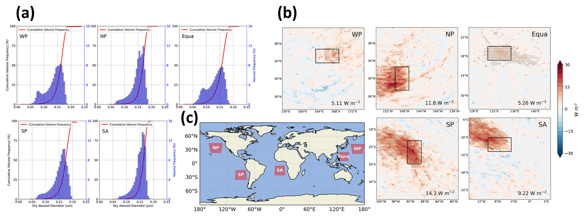
Figure 1 Injecting sea salt aerosols into five open-ocean regions to simulate the implementation of MCB geoengineering. (a) The cumulative volume frequency of increased aerosol dry-particle size (uniform injection of 10⁻⁹ kg m⁻² s⁻¹ sea salt aerosols over the entire region). (b) Difference (Exp − Base) in the spatial distribution of the TOA upward shortwave radiative flux response (SW_TOT) resulting from uniform injection of 10⁻⁹ kg m⁻² s⁻¹ of sea salt aerosol in sensitive areas of the five ocean regions, with SW_TOT response values resulting only in the sensitive areas labeled in the lower-right corner. Areas labeled with dots indicate mean differences that are significant at the 95 % confidence level. The black rectangles are sensitive areas. (c) Locations of the five ocean modeling domains.

The grids of WRF and CMAQ are 190 × 190 and 173 × 173, respectively, and both have a horizontal resolution of 12 km, with 29 vertical layers from the surface to an altitude of about 21 km. The simulation period for the WP, Equa, and NP regions in the Northern Hemisphere is from 24 July to 1 September 2018, while for the SP and SA regions in the Southern Hemisphere the simulation period is from 24 February to 1 April 2023. The first 8 d of the model simulations are considered the spinup period in order to minimize the impacts of the initial chemical conditions.

Figure 2 Column mean liquid cloud fraction from the surface to an altitude of 3000 m for the five regions. The first to fourth columns are Base, the sensitivity experiment with a uniform injection of 10⁻⁹ kg m⁻² s⁻¹ sea salt aerosols over the entire region, Exp − Base, and the percent change of Exp − Base, respectively.

Table 1 The cloud fraction, CDNC, LWP, and regional sea salt aerosol concentrations at Base and after injection of sea salt aerosols at 10⁻⁹ kg m⁻² s⁻¹ (Exp) for the five ocean regions.

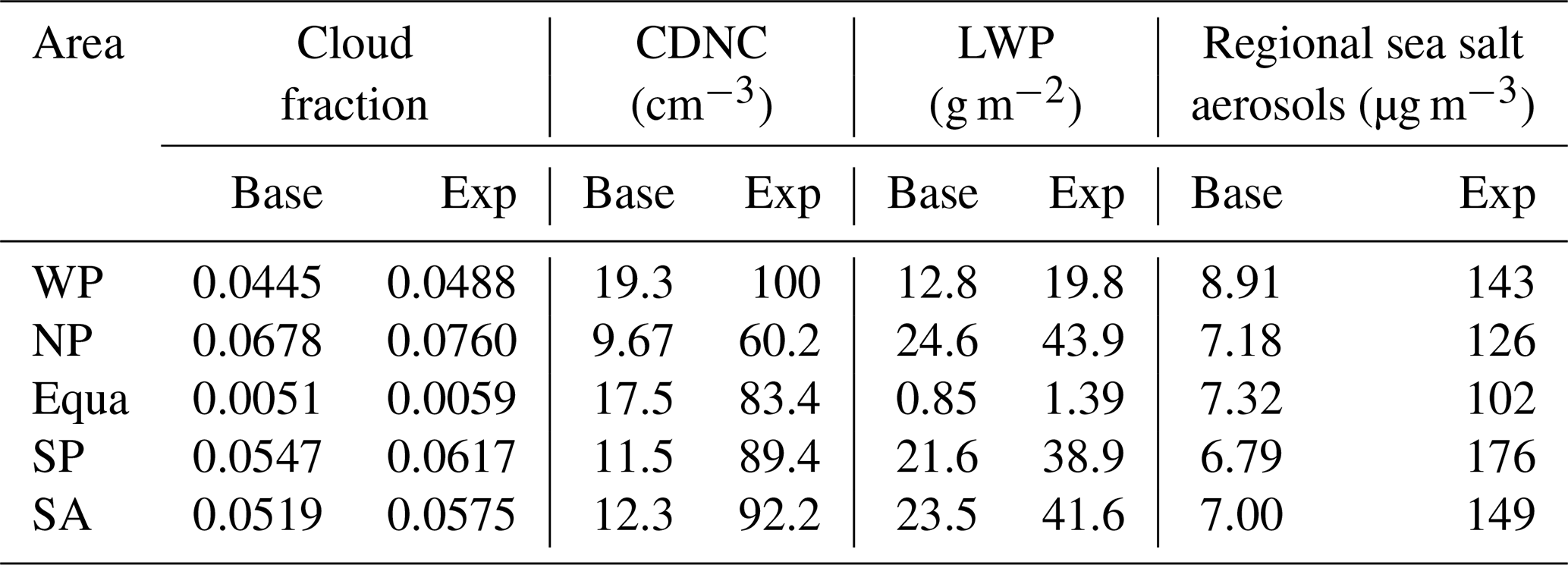
The results of the Base simulations with the model settings described above and the default sea salt emissions (no aerosol injection) were obtained. As can be seen, there are significant differences in the cloud distributions for the five ocean regions in the Base simulations during the study period, with wider distributions of liquid clouds in the NP, SP, and SA regions but fewer clouds in the WP and Equa regions (Fig. 2, first column). The cloud heights are distributed between 500 and 2000 m and centered at 1000 m (Fig. S1, first column). The cloud fraction, CDNC, liquid water path (LWP), and sea salt aerosol concentrations in the Base simulations for each region are summarized in Table 1.

We test four different sea salt aerosol injection strategies, i.e., wind-speed-dependent Natural × 5, Wind-adjusted, Fixed at 10⁻⁹ kg m⁻² s⁻¹, and Fixed-wind-adjusted. All additionally injected sea salt aerosols are in accumulation mode. In this study, the geometrical mean dry diameter of sea salt aerosols injected into the five regions is about 0.11–0.15 µm and is similar for all the emission scenarios.

Natural × 5: increase the emission rates of accumulation-mode sea salt aerosols by a factor of 5 (Hill and Ming, 2012). This is a simple wind-speed-dependent increase. The injection rates in the five regions are equivalent to 0.031–0.085 × 10⁻⁹ kg m⁻² s⁻¹ (Table S2).

Wind-adjusted: Salter et al. (2008) designed a spray vessel for injecting sea salt aerosols with a spray efficiency that was dependent on wind speed and was expected to achieve maximum spray outputs at wind speeds between 6 and 8 m s⁻¹. The threshold wind speed was set to 7 m s⁻¹ and the spray efficiency at lower wind speeds raised to the power of 1.5. We use the source function of Partanen et al. (2012) as follows, where u is the 10 m wind speed. For example, at a wind speed of 7 m s⁻¹, the injection rate will be 0.26 × 10⁻⁹ kg m⁻² s⁻¹:

$$\begin{array}{}\text{(3)}& F_{\mathrm{m},\mathrm{baseline}}=\left\{\begin{array}{l}\mathrm{5}\times \mathrm{2.8}\times {\mathrm{10}}^{-\mathrm{12}}\times {\left(\frac{u}{\mathrm{1}\mathrm{m}{\mathrm{s}}^{-\mathrm{1}}}\right)}^{\mathrm{1.5}}\mathrm{kg}{\mathrm{m}}^{-\mathrm{2}}{\mathrm{s}}^{-\mathrm{1}},\\ u<\mathrm{7}\mathrm{m}{\mathrm{s}}^{-\mathrm{1}},\\ \mathrm{5}\times \mathrm{2.8}\times {\mathrm{10}}^{-\mathrm{12}}\times {\mathrm{7}}^{\mathrm{1.5}}\mathrm{kg}{\mathrm{m}}^{-\mathrm{2}}{\mathrm{s}}^{-\mathrm{1}},\\ u\ge \mathrm{7}\mathrm{m}{\mathrm{s}}^{-\mathrm{1}}.\end{array}\right.\end{array}$$

Fixed at 10⁻⁹ kg m⁻² s⁻¹: unlike the previous two injection methods, the injections of sea salt aerosols at a fixed rate of 10⁻⁹ kg m⁻² s⁻¹ are not dependent on wind speed and increased uniformly over all the ocean grids. Injecting sea salt aerosols at a fixed rate identified the geographic areas that were most sensitive to increased sea salt aerosols and produced the largest top-of-atmosphere (TOA) radiative perturbations (Alterskjær et al., 2012). Many other studies have used this method (Goddard et al., 2022; Horowitz et al., 2020; Mahfouz et al., 2023). Uniform injections of sea salt aerosols throughout the region ignored aerosol transport and dispersion at the boundary. Therefore, based on the results of a fixed 10⁻⁹ kg m⁻² s⁻¹ injection rate, we identified the geographical regions (30 × 50 grid points approximately 360 km × 600 km away from the domain boundary) in the five ocean areas where the TOA radiative perturbations caused by uniform injection were largest and most sensitive. Table S3 shows the locations of these sensitive regions. The injection amount in a sensitive region at a fixed 10⁻⁹ kg m⁻² s⁻¹ injection rate is found to be about $\mathrm{1}/\mathrm{20}$ of that in the full domain.

Fixed-wind-adjusted: to rule out differences in radiative and cloud responses due to wind variabilities in spray rates, we perform an additional adjustment. Similar to Natural × 5, the injections of sea salt aerosols are also dependent on the wind speed, but the integrated amounts in the region are set to be equal to the case where all the areas had a fixed rate of 10⁻⁹ kg m⁻² s⁻¹ (fixed).

2.3 Calculations

The calculation method related to radiation, cloud properties, and cloud radiation forcing is based on Goddard et al. (2022) and is briefly described here as follows. This study focuses on the shortwave radiative flux responses at the TOA due to the injections of sea salt aerosols, which is consistent with the definition of effective radiation forcing (ERF) (Forster et al., 2007). The sea surface temperature in the model is preset by NCEP-FNL, so the model's surface temperature and upward longwave radiation would not respond to the increased sea salt aerosols. The total upward shortwave radiation flux (SW_TOT) at the TOA is under the all-sky conditions. The responses of SW_TOT to the injections of sea salt aerosols could be divided into cloud radiative effects (SW_CLD, excluding the direct effect of aerosols) and direct scattering effects when clouds are present (SW_AER).

$$\begin{array}{}\text{(4)}& \mathrm{SW}\mathit{\_}\mathrm{TOT}=\mathrm{SW}\mathit{\_}\mathrm{CLD}+\mathrm{SW}\mathit{\_}\mathrm{AER}\end{array}$$

The diagnosis of a clean sky (no aerosols) is not considered in the previous WRF–CMAQ model. So, in this study, we extend this feature of the WRF–CMAQ model using the methodology of Ghan et al. (2012) and performing a double-radiative call at each time step to calculate radiation variables related to a clean sky (SW_CLD). We also study the impacts of injecting sea salt aerosols on the upward shortwave radiation flux at the TOA under the clear-sky conditions (SW_AER_CLR). For this flux, only the direct scattering effect of aerosols exists as clouds are ignored, which is considered to be the maximum MSB potential generated by injecting sea salt aerosols when there is no cloud.

Due to the different amounts of sea salt aerosols injected by the four different injection strategies, we propose the concept of MCB efficiency (E_MCB) to measure the relationships between the number of sea salt aerosol injections and the resulting radiation flux responses (Table S2).

$$\begin{array}{}\text{(5)}& E_{\mathrm{MCB}}={\displaystyle \frac{\begin{array}{c}\mathrm{\text{SW\_TOT response due to injection of}}\\ \mathrm{\text{sea salt aerosol }}\left(\mathrm{W}{\mathrm{m}}^{-\mathrm{2}}\right)\end{array}}{\text{sea salt aerosol injections }\left(\mathrm{kg}{\mathrm{m}}^{-\mathrm{2}}{\mathrm{s}}^{-\mathrm{1}}\right)}}\end{array}$$

This is a measure of the mass efficiency of MCB implementation in different regions, i.e., the extent to which the SW_TOT responses are expected to be generated by injecting sea salt aerosols at a rate of 1 kg m⁻² s⁻¹. E_MCB = 1 means that injecting 1 kg of sea salt aerosols per unit time is expected to produce a 1 GW (10⁹ W) SW_TOT response. Note that this value (E_MCB) is based on model calculations under specific atmospheric conditions within the study region and is only used to analyze the sensitivities of the radiative flux to different injection methods and injection amounts.

This study focuses on the changes in liquid clouds and evaluates the responses in cloud condensation nuclei (CCN), cloud fraction, CDNC, r_e, LWP, cloud optical thickness (COT), and cloud albedo due to the injections of sea salt aerosols. These calculations are shown in Sect. S1.

Cloud radiation forcing (CRF) parameters can be used to quantify the responses of SW_CLD to changes in cloud cover or cloud albedo, defined as follows (Goddard et al., 2022):

$$\begin{array}{}\text{(6)}& {\mathrm{CRF}}_{\mathrm{param}}={\mathit{\alpha }}_{\mathrm{c}}f,\end{array}$$

where α_c is the mean cloud albedo and f is the mean cloud fraction.

The CRF parameters can be approximated using the perturbation method as follows (Goddard et al., 2022):

$$\begin{array}{}\text{(7)}& {\mathrm{CRF}}_{\mathrm{param}}^{\prime }={\mathit{\alpha }}_{\mathrm{c}}^{\prime }\stackrel{\mathrm{‾}}{f}+{\stackrel{\mathrm{‾}}{\mathit{\alpha }}}_{\mathrm{c}}{f}^{\prime }+{\mathit{\alpha }}_{\mathrm{c}}^{\prime }{f}^{\prime },\end{array}$$

where the first term on the right-hand side indicates the changes in CRF_param driven by the perturbation of the cloud albedo, the second term indicates the changes driven by the perturbation of the cloud fraction, and the third term denotes the changes driven by the interactions between the two. The horizontal bars on α_c and f are defined as the monthly mean of the Base, and the prime (^′) defines the monthly mean differences between the sensitivity experiments and the Base. The fourth column of Fig. S17 shows that the differences between CRF_param and CRF${}_{\mathrm{param}}^{\prime }$ are small enough that the perturbation method can be used to approximate CRF${}_{\mathrm{param}}^{\prime }$.

The changes in cloud albedo are driven by multiple processes. Based on Quaas et al. (2008) and Christensen et al. (2020), Goddard et al. (2022) formulated the following equation to assess the relative effects of CDNC, LWP, and mean cloud fraction on the responses of SW_CLD due to the injections of sea salt aerosols:

$$\begin{array}{}\text{(8)}& \begin{array}{rl}& {\displaystyle \frac{\mathrm{\Delta }\mathit{\alpha }}{\mathrm{\Delta }\ln \mathrm{AOD}}}=f\mathrm{\Delta }{\mathit{\alpha }}_{\mathrm{c}}\left(\mathrm{1}-{\mathit{\alpha }}_{\mathrm{c}}\right)\\ & \left({\displaystyle \frac{\mathrm{1}}{\mathrm{3}}}{\displaystyle \frac{\mathrm{\Delta }\ln \mathrm{CDNC}}{\mathrm{\Delta }\ln \mathrm{AOD}}}+{\displaystyle \frac{\mathrm{5}}{\mathrm{6}}}{\displaystyle \frac{\mathrm{\Delta }\ln \mathrm{CLWP}}{\mathrm{\Delta }\ln \mathrm{AOD}}}+{\displaystyle \frac{\mathrm{\Delta }\ln f}{\mathrm{\Delta }\ln \mathrm{AOD}}}\right),\end{array}\end{array}$$

where α is the planetary albedo, Δ represents the difference in monthly average results between the sensitivity experiments and Base simulations, and α_c is the cloud albedo. The three terms inside the parentheses represent the relative contributions of the Twomey effect, LWP effect, and cloud fraction effect, respectively, with the latter two related to the second aerosol indirect effect (Albrecht, 1989).

Additional statistics are obtained by generating three ensemble members for each experiment in each region using a stochastic kinetic-energy backscatter scheme to add stochastic perturbations (Berner et al., 2011). A two-tailed t test was applied to assess whether the difference between the Base simulation and the experiment was statistically significant at the 95 % confidence level. Unless specified otherwise, all the results in this study are shown as overall regional monthly averages of the ensemble.

3 Results

3.1 The impacts of different injection strategies on shortwave radiation at the TOA

In modeling studies, variations in the methods used to increase sea salt aerosols may lead to different conclusions, and these variations may be one of the reasons for differences in the assessments of MCB potentials in previous studies. In this study, sea salt aerosols injected following different strategies (with dry diameters of about 0.11–0.15 µm; Fig. 1a) increase the SW_TOT at the TOA by 0.07–25 W m⁻² in the five ocean regions compared with the Base experiment (Fig. 3a). The natural × 5 and wind-adjusted strategies, which rely on wind speeds, inject sea salt aerosols of 0.031–0.085 and 0.18–0.21 × 10⁻⁹ kg m⁻² s⁻¹ into the five regions and result in SW_TOT variations of 0.07–2.1 and 1.4–8.4 W m⁻², respectively (Fig. 3a and Table 2). Uniform injections of sea salt aerosols at a fixed rate of 10⁻⁹ kg m⁻² s⁻¹ result in SW_TOT changes of 11–25 W m⁻² in the five regions. The three stratocumulus regions NP, SP, and SA have the most significant SW_TOT responses, all exceeding 20 W m⁻², while the SW_TOT responses in the WP and Equa regions are 18 and 11 W m⁻², respectively.

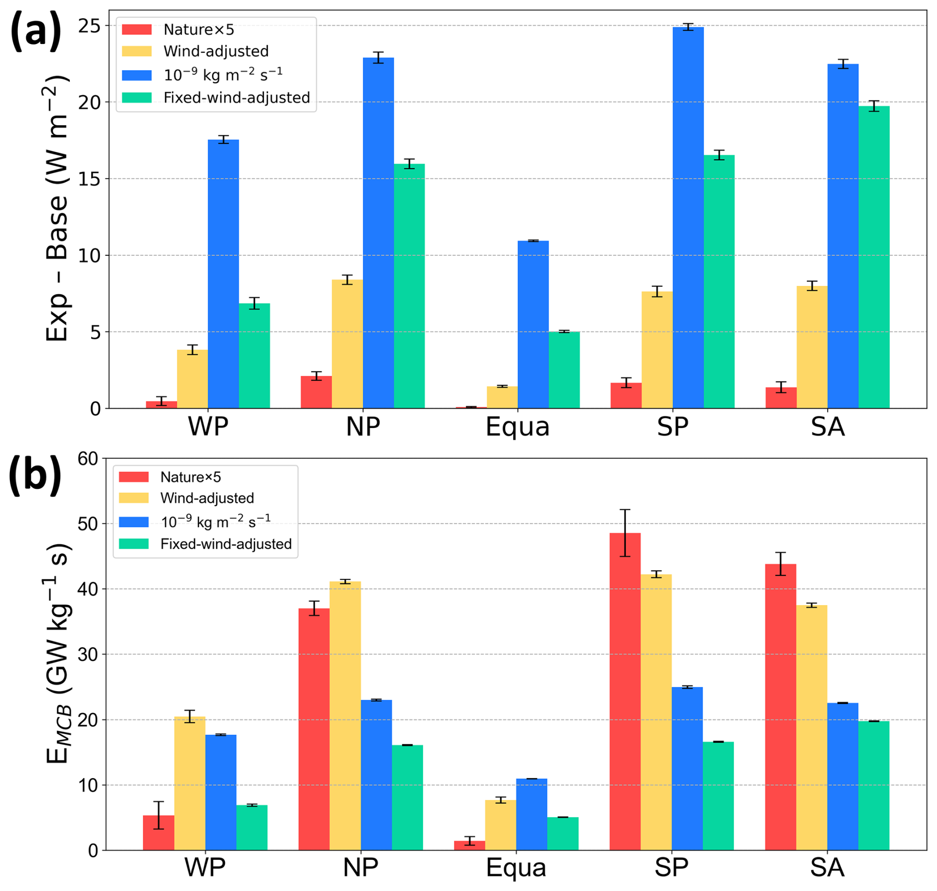
Figure 3 (a) The differences in SW_TOT and (b) MCB efficiency (E_MCB) due to the injection of sea salt aerosols following different strategies in the five ocean regions.

Table 2 Differences (Exp − Base) in SW_TOT, SW_CLD, SW_AER, and SW_AER_CLR at the TOA due to the injection of sea salt aerosols following different strategies in the five ocean regions.

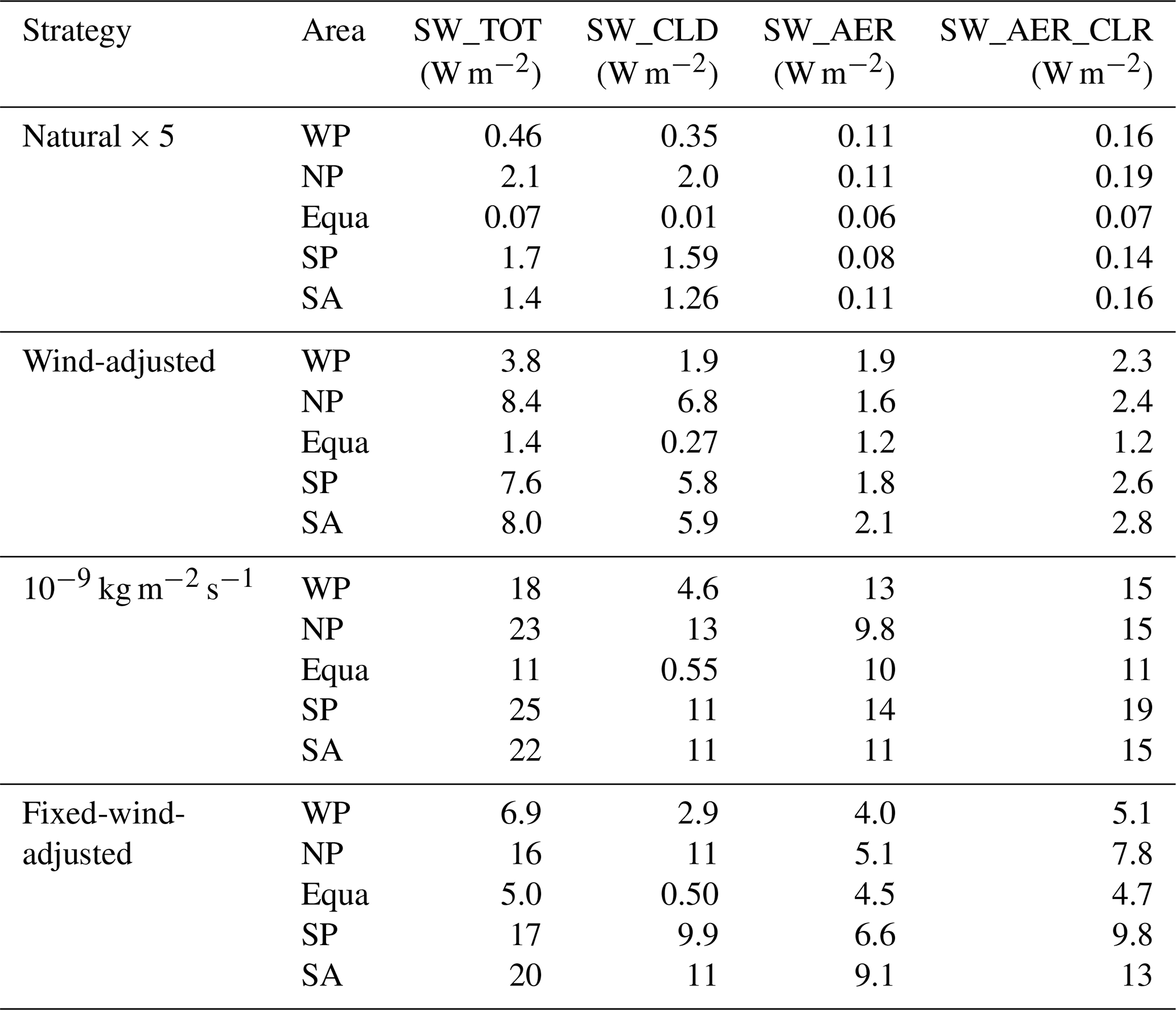
Note: SW_TOT is the upward shortwave radiative flux at the TOA for all-sky conditions. The response of SW_TOT to the sea salt aerosol injection can be separated into the influence of the cloud radiative effect (SW_CLD, where the influence of the aerosol is excluded) and the influence of the aerosol direct scattering effect (SW_AER) in the presence of clouds. That is, SW_TOT = SW_CLD + SW_AER. SW_AER_CLR is the response of aerosol direct scattering to the upward shortwave radiative flux at the TOA under clear skies.

Injecting the same amount of sea salt aerosols results in substantial variations in SW_TOT responses across the different regions (Fig. S2). The sea salt aerosols sprayed in the Fixed-wind-adjusted experiments are also dependent on wind speed, but the emission rate integrated in the full domain is consistent with the fixed rate of 10⁻⁹ kg m⁻² s⁻¹, ruling out the differences caused by the amount of injected sea salt aerosols. Although both strategies inject the same amounts of sea salt aerosols, the SW_TOT responses they produce are significantly different. The Fixed-wind-adjusted strategy results in SW_TOT changes of 5.0–20 W m⁻² in the five regions (Fig. 3a), indicating that the shortwave radiation flux changes caused by wind-speed-dependent injections are smaller than those caused by uniform injections and show regional differences.

Figure 3b shows the E_MCB values of the different sea salt injection strategies in the five regions. Overall, MCB implementation is more efficient in the NP, SP, and SA regions, while it is less efficient in WP and Equa, which is similar to the previous SW_TOT response results. E_MCB also varies for the different injection strategies. In the NP, SP, and SA regions, the E_MCB values of the Natural × 5 and Wind-adjusted strategies with relatively small injection amounts are higher than for the other two strategies with large injection amounts. For the same injection amount, injecting at a fixed rate shows a higher E_MCB value relative to injections depending on wind speed, as consistently shown in all five regions (Fig. 3b). Since the number flux of the aerosols increased with the decreases in the injected aerosol particle size for the same mass flux, we examined the MCB efficiency in units of aerosol number concentration (Fig. S3). The results showed a higher MCB number efficiency with less aerosol number flux injected (Fig. S3c). For the same quantity injected, the aerosol number varied greatly (Fig. S3d) and the MCB number efficiency was higher for Fixed-wind-adjusted injection than for uniform injection (Fig. S3c).

The production of sea salt aerosols in nature is strongly correlated with wind speed, and most models associate sea salt aerosol emissions with wind speed (Ahlm et al., 2017; Grythe et al., 2014). Injection strategies depending on wind speed bring the distributions of added sea salt aerosols closer to natural distributions. In natural environments, sea salt aerosol emissions in strong-wind areas (e.g., storm or typhoon areas) and surf zones are usually much higher than in weak-wind areas. Therefore, injection strategies depending on wind speed concentrate the added sea salt aerosols in strong-wind areas and surf zones, while the weak-wind regions increase sea salt aerosols relatively little (Fig. S4). Injecting uniformly at a fixed rate in the model will result in a large increase in sea salt aerosols in places with initially low aerosol concentrations (e.g., weak-wind regions). This strategy may not truly reflect the distribution characteristics of the natural environment. However, the uniform increase injection strategy also has its advantages: not only can it avoid a lower increase in sea salt emissions in regions with lower wind speeds, but it can also identify the geographical areas that are most sensitive to the increased sea salt aerosols and that produce the largest TOA radiation perturbations (Alterskjær et al., 2012). Therefore, when using models to simulate the injections of sea salt aerosols by increasing the emission rate, it is necessary to fully consider the impact of different injection strategies on the distribution of sea salt emissions and to choose a suitable strategy for the purpose of the study.

Injecting sea salt aerosols in the sensitive areas with the same uniform injections (10⁻⁹ kg m⁻² s⁻¹; the injection amount is about $\mathrm{1}/\mathrm{20}$ of the full domain injection) results in changes of 0.49–3.4 W m⁻² in SW_TOT in the five ocean regions (Table S2). The SW_TOT responses are largest in the SP region, at 3.4 W m⁻², and 2.7 and 1.7 W m⁻² in the NP and SA regions, respectively, while they are only 0.49 and 0.83 W m⁻² in the WP and Equa regions, respectively. The injected sea salt aerosols produced SW_TOT changes of 5.11–14.3 W m⁻² in the sensitive areas (Fig. 1b). Similarly, the increases in SW_TOT in the SP, SA, and NP regions all exceeded 9 W m⁻², with the highest increase in the SP region at 14.3 W m⁻². In the WP and Equa regions, the increases in SW_TOT are 5.11 and 5.26 W m⁻², respectively. Considering that the original intents of MCB or MSB design were regional applications (hurricane mitigation, coral reef protection, and polar sea ice recovery) (Latham et al., 2014), choosing to inject sea salt aerosols in the sensitive areas could achieve the corresponding cooling goals within the region and also affect larger areas through the diffusion and transport of aerosols.

3.2 Characterization of the radiation responses

SW_TOT responses are defined as the sum of the upward shortwave radiation flux response at the TOA generated by the combined effects of the direct scattering effect of aerosols (SW_AER) and cloud radiative effects (SW_CLD) after injecting sea salt aerosols. Figure 4 shows the contributions of SW_AER and SW_CLD responses in SW_TOT produced by different injection strategies in the five ocean regions. The majority of the SW_TOT radiative flux response due to the lower mass injection Natural × 5 and Wind-adjusted strategies is caused by the SW_CLD response (Fig. 4a). In the NP, SP, and SA regions, the contributions of SW_CLD exceed 70 %, suggesting that sea salt aerosols injected at these locations increase SW_TOT mainly by affecting clouds through indirect effects. In Equa, the responses of SW_TOT are entirely caused by SW_AER. This is due to the low cloud cover in Equa (Fig. 2i), so the SW_CLD caused by the aerosol injection is small here. The proportion of SW_AER produced by the uniform injection of sea salt aerosols at a fixed rate of 10⁻⁹ kg m⁻² s⁻¹ continued to increase (Fig. 4c). In the WP, Equa, and SP regions, the proportion of SW_AER exceeded that of SW_CLD. In the SA region, SW_CLD and SW_AER are almost equal, while in the NP region the SW_CLD response is 13 W m⁻², which is still greater than SW_AER (9.8 W m⁻²). This is because there is a saturation phenomenon in the cloud response to aerosol injections (discussed below), and the NP, SP, and SA regions provide more SW_CLD responses, while the cloud responses in the WP and Equa regions saturate and no longer increase. The results of the Fixed-wind-adjusted case show that, for the same injection amount, the SW_AER responses caused by the injection strategy that relies on wind speed are significantly smaller than those of the method with fixed-rate uniform injection, while the disparity in the SW_CLD responses is minimal. This is mainly because fixed-rate uniform injection leads to a larger aerosol number flux (Fig. S3d). In addition, the injection strategy that relies on wind speed distributed most of the increased sea salt aerosols to areas with already high emissions, such as strong-wind areas and surf zones, where the excess marine aerosols have already saturated the cloud responses, resulting in minor changes in SW_CLD. In areas with weak winds, the potentials for direct aerosol scattering are not fully exploited due to the relatively small amounts of sea salt aerosols injected, leading to a lower SW_AER response.

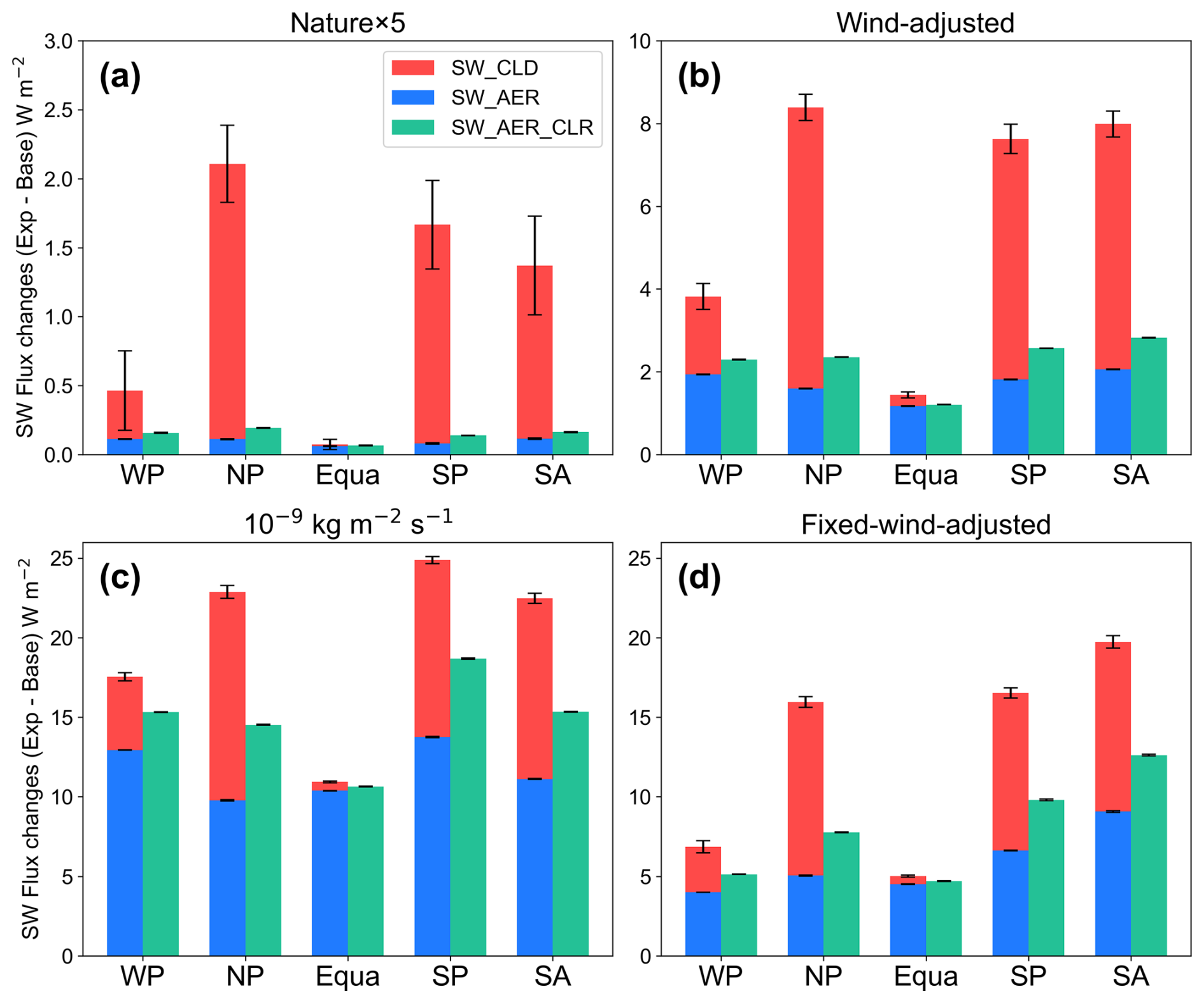
Figure 4 Decomposition of the upward shortwave radiative fluxes at the TOA due to the different strategies for injecting sea salt aerosols in the five regions. Note that the y-axis ranges are not consistent.

Figures S5 and S6 show the spatial distributions of SW_CLD and SW_AER responses resulting from the different injection methods in the five ocean regions. The SW_CLD responses are stronger in the three regions of NP, SP, and SA, while they are weaker in the regions of WP and Equa, and in some locations they even lead to a reduction in the upward shortwave radiation (Fig. S5). The spatial distributions of the SW_CLD responses exhibit noticeable differences, reflecting significant regional differences in the non-uniform distributions of clouds and their impacts on shortwave radiation at the TOA. The effect of cloud properties on SW_CLD will be shown in Sect. 3.5. Due to the influences of various complex factors on cloud formations and distributions, simulation results related to clouds show significant spatial variabilities. This might be the result of the combined effects of local meteorological conditions and changes in cloud physical properties caused by sea salt aerosol injections.

In contrast, the spatial distributions of the SW_AER response are smoother, leading to consistent increases in upward shortwave radiation at the TOA in all the ocean regions (Fig. S6). This indicates smaller spatial limitations in the distributions of aerosol particles, allowing direct scattering effects to take place everywhere. The direct scattering effect of aerosols is primarily related to the concentrations and physical properties of the particles (discussed below), unlike clouds, which are influenced by multiple variables. These results suggest that, when implementing geoengineering measures, it is essential to comprehensively consider the interactions between aerosols and clouds as well as their different response patterns in various regions.

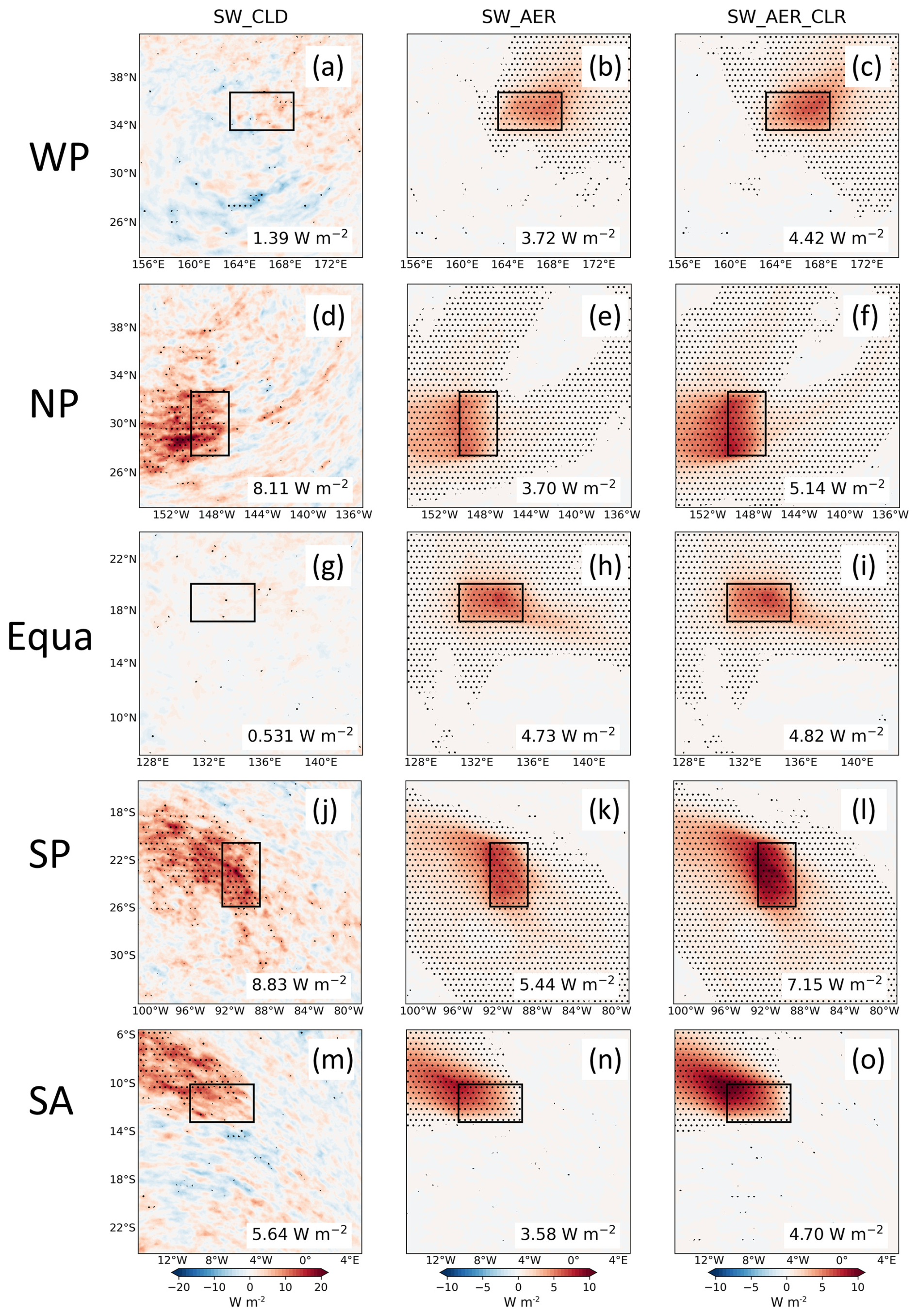
Figure 5 Spatial distribution of SW_CLD (first column), SW_AER (second column), and SW_AER_CLR (third column) responses resulting from the injection of 10⁻⁹ kg m⁻² s⁻¹ of sea salt aerosols in the sensitive areas over the five ocean regions. The values of the radiative flux responses generated only in the sensitive area are labeled in the lower-right corner. Areas labeled with dots indicate mean differences that are significant at the 95 % confidence level. The black rectangles are the sensitive areas.

The SW_CLD response resulting from the injection of sea salt aerosols in the sensitive areas of the five ocean regions exhibits significant spatial differences. The SW_CLD response is larger than the SW_AER response in the sensitive areas of NP, SP, and SA, indicating that the changes in SW_TOT are mainly driven by the cloud radiative response (Fig. 5). In contrast, the SW_CLD response is smaller in the WP and Equa regions. This is because of the low cloud cover in Equa, and it is also worth noting that the cloud in WP is centrally distributed in the northern part of the region and that its SW_CLD response is larger in the north. This regional difference is similar to that observed with uniform injection across the entire region. The SW_AER response shows consistent results in all the areas, resulting in a radiation response change of 3.58–5.44 W m⁻² within the injection areas. In WP and Equa, the variations in SW_TOT are primarily driven by the direct scattering effects of aerosols. Aerosols can have a greater impact on radiation responses outside the sensitive areas through transports and diffusions, reaching up to 3 times the total radiation within the sensitive areas (Fig. 6). In all the regions except WP, the total SW_CLD response outside the sensitive region was about 270 %–408 % higher than inside. In WP, the SW_CLD response outside the sensitive area has a negative effect. The SW_CLD responses in NP, SP, and SA extend to the west and northwest of the injection due to the prevailing winds, indicating that clouds in these areas are affected by the injection of sea salt aerosols (Fig. 5). Changes in cloud microphysical properties will be presented later. The SW_CLD variations in other directions are not uniform, and there are negative SW_CLD responses in some grids, which again reflects the spatial complexities of cloud radiative effects. The direct scattering effects of aerosols on areas outside the sensitive region is reflected in a widespread increase in upward shortwave radiation at the TOA. The total SW_AER responses outside the sensitive areas in the five ocean regions are approximately 160 %–281 % higher than inside but lower than the impacts of SW_CLD responses outside the sensitive areas. The SW_AER and SW_CLD responses have similar spatial distributions due to the transport of the aerosols.

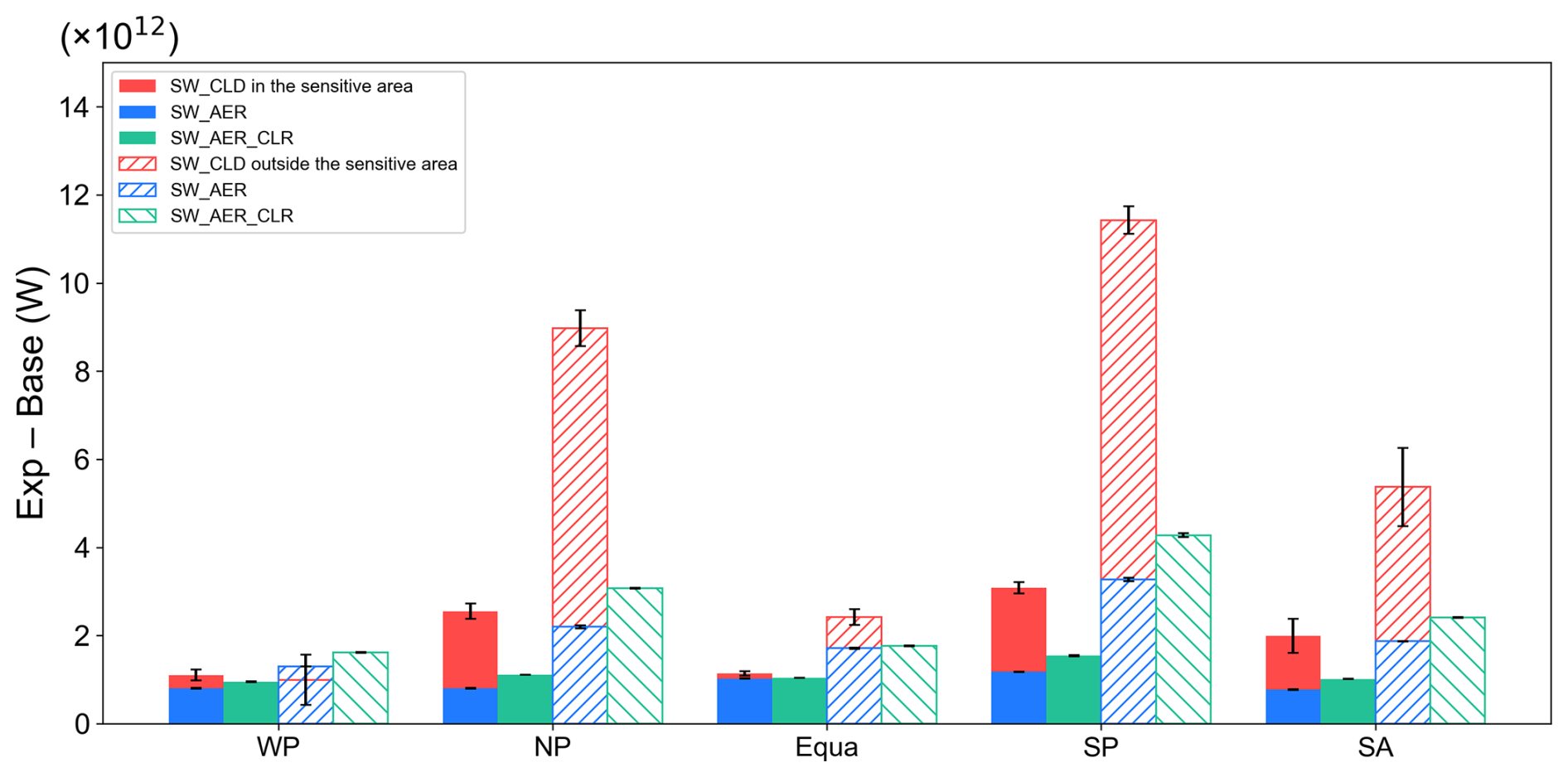
Figure 6 Total SW_CLD, SW_AER, and SW_AER_CLR responses resulting from the injection of 10⁻⁹ kg m⁻² s⁻¹ of sea salt aerosols within the sensitive areas of the five regions. The solid columns indicate the total radiative response calculated for aerosol injection within the sensitive areas. Columns filled with hatching indicate the total radiative response outside the sensitive areas.

3.3 Saturation of the cloud radiative responses

Figure 7 shows that, with low levels of sea salt aerosol injections, radiation response changes are mainly driven by SW_CLD responses. As the injected sea salt aerosols increase, the SW_CLD responses gradually reach saturation. After reaching a certain injection level, the increases in the SW_CLD responses stabilize at their maximum value and no longer increase with further injections. The SW_CLD responses show large differences in the five ocean regions, and the different shapes and slopes of the curves indicate that the cloud radiative forcing responses to the sea salt aerosol injections are different in each region. This might be due to variations in cloud types, cloud amounts, and atmospheric conditions in the different regions. In NP, SP, and SA, the SW_CLD responses exceed 10 W m⁻², while in WP they saturate at 5 W m⁻². In Equa, when the sea salt aerosol injection rate is 10⁻⁹ kg m⁻² s⁻¹, the SW_CLD response is 0.5 W m⁻², and even when the injection rate is doubled the SW_CLD response remains at 0.5 W m⁻². This implies that SW_TOT at Equa comes almost exclusively from the contributions of the direct scattering effects of aerosols.

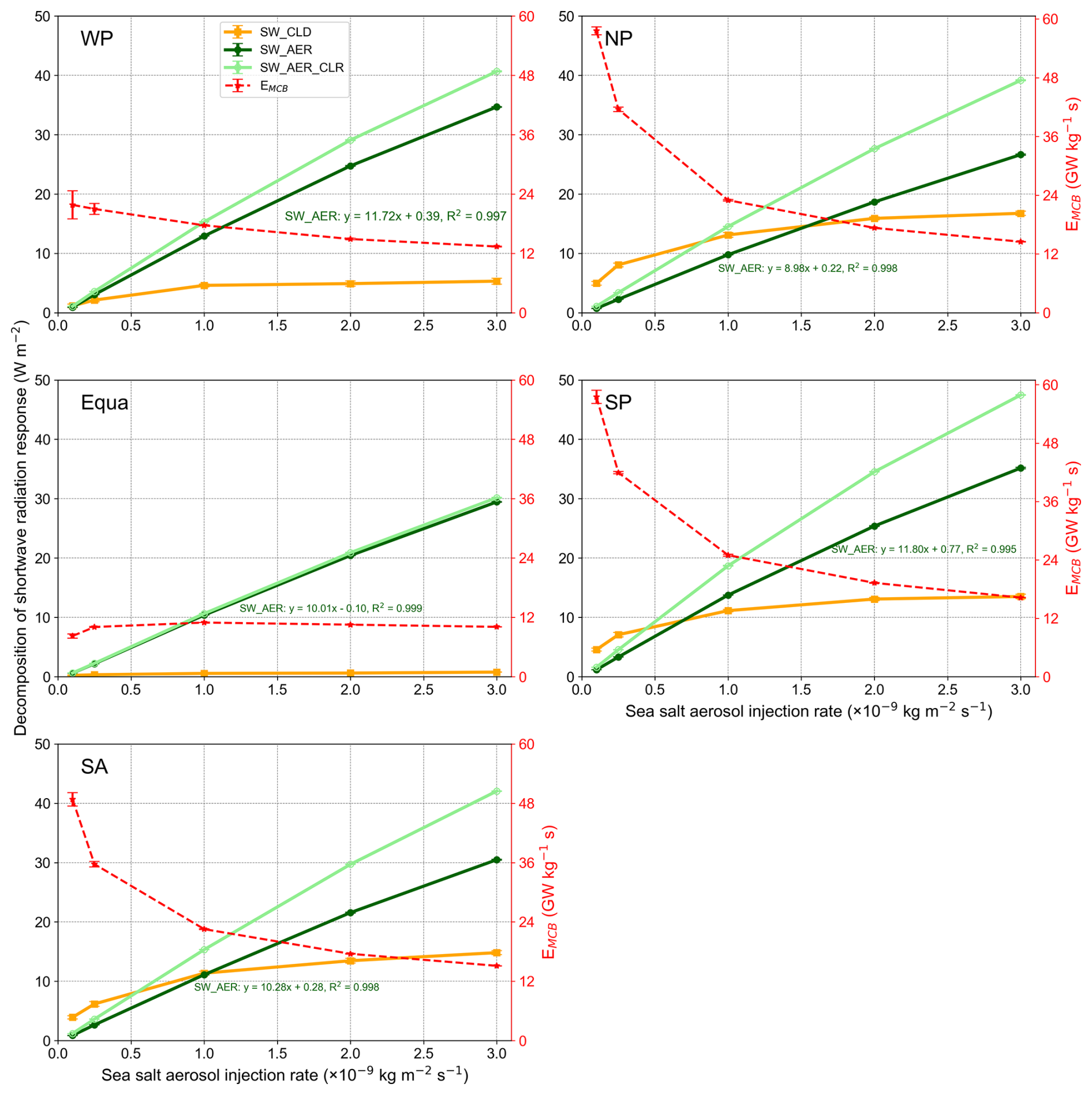
Figure 7 Changes in SW_CLD, SW_AER, and SW_AER_CLR radiative responses due to sea salt aerosols uniformly injected in varying amounts in the five ocean regions, together with the corresponding changes in E_MCB. SW_AER and SW_AER_CLR are labeled with the results of the corresponding linear regression analysis. The error bars reflect the ensemble spread.

In contrast to SW_CLD, the SW_AER responses increase linearly with the injections of sea salt aerosols (R² > 0.99). As the injection increases, the contributions of SW_AER to SW_TOT gradually increase, surpassing the SW_CLD responses, and show the same trends across the five regions. This implies that, at higher injection levels, the contributions of SW_CLD to the total radiation change saturate, and the cloud properties no longer change significantly. At this point, sea salt aerosols primarily affect radiation through direct scattering effects, and the aerosol particles' ability to scatter solar radiation continues to increase with the increases in aerosol quantities. In some cloud-free regions or weather conditions, injected sea salt aerosols are still able to cool through direct scattering.

There exists a specific injection level at which the SW_CLD and SW_AER responses are equal. In the NP region, when the injection level is approximately 1.55 × 10⁻⁹ kg m⁻² s⁻¹, both the SW_CLD and SW_AER responses are 15 W m⁻². In SP and SA, these levels are about 0.67 × 10⁻⁹ and 1 × 10⁻⁹ kg m⁻² s⁻¹, respectively, while in WP the responses were already equal when the injection amount was 0.15 × 10⁻⁹ kg m⁻² s⁻¹. Since there is a saturation of the cloud radiative effects, E_MCB decreases with the increases in sea salt aerosol injection amounts (Fig. 7, red dashed line). This can also explain the higher E_MCB value of the Natural × 5 and Wind-adjusted strategies with relatively low injection amounts (Fig. 3b). The lower E_MCB value of the Fixed-wind-adjusted injection relative to the fixed uniform injection therefore indicates that wind-dependent injection strategies lead to the injection of large amounts of sea salt aerosols in certain areas with high wind speeds, leading to saturation of cloud radiative effects, which might affect the performances of MCB in simulations of regional and global models.

When fewer sea salt aerosols are injected, both the SW_CLD and SW_AER responses contribute to the changes in SW_TOT. As the injection amounts increase, the SW_CLD responses saturate, and the increases in SW_TOT depend on the increases in the SW_AER responses, leading to a decrease in E_MCB (Fig. 7). Therefore, implementing geoengineering with sea salt aerosol injections requires consideration of local atmospheric conditions and balancing of the relationships between cooling goals and sea salt injection efficiencies.

Under clear-sky and cloudless conditions, injecting sea salt aerosols could still increase SW_TOT through direct scattering, and this effect exceeds those of aerosol direct scattering when clouds are present. The variation of the upward shortwave radiation flux at the TOA under the clear-sky conditions (SW_AER_CLR) does not exhibit significant regional heterogeneity across the ocean areas (Figs. 5 and S7), suggesting that the contribution of direct aerosol scattering is more uniform globally when considering the effects of sea salt injections on Earth's radiation budget. The SW_AER_CLR responses are also linearly correlated with the injection of sea salt aerosols (R² > 0.99), and they exceed the SW_AER responses (Fig. 7). This is because cloud layers also scatter and absorb solar radiation, so this scattering effect is more significant under clear-sky conditions. This is reflected in the fact that, in regions with higher cloud fractions, such as the NP, SP, and SA regions, the differences between the SW_AER and SW_AER_CLR responses are also larger (Fig. 7). When injecting sea salt aerosols in sensitive areas, the spatial distributions of the SW_AER_CLR and SW_AER responses are very consistent (Fig. 5). Therefore, injecting sea salt aerosol under conditions of low cloud cover or clear skies also increases the upward shortwave radiation flux at the TOA.

3.4 Factors affecting the radiation effects

Uniform injections of 10⁻⁹ kg m⁻² s⁻¹ of sea salt aerosols lead to an increase in aerosol optical depth (AOD) of 0.20–0.37 in all the regions (Fig. 8). The distributions of AOD within the regions are not uniform due to aerosol transports and diffusions, with some areas showing an increase in AOD of over 0.6. Injecting sea salt aerosols in sensitive areas leads to an AOD increase of 0.077–0.12, while outside the injection areas AOD gradually decreases as the aerosols are transported and disperse. With the increases in sea salt aerosol injections, AOD shows a linear increase within a certain range in all five ocean regions (R² > 0.998; Fig. 9a).

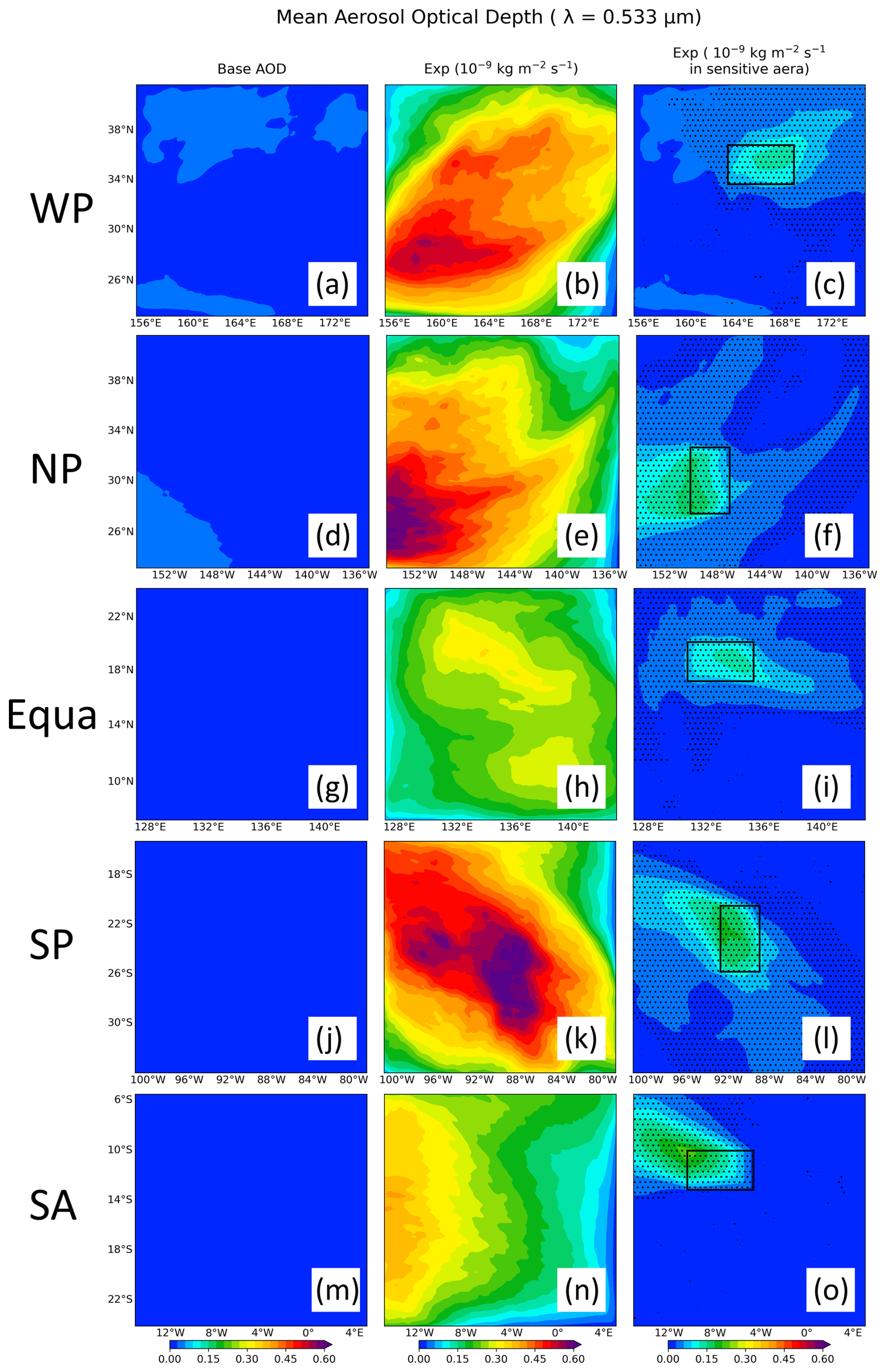
Figure 8 Spatial distribution of the mean AOD (λ=0.533 µm) for the five ocean regions. The first column is the AOD for Base, the second column is the AOD after uniform injection at 10⁻⁹ kg m⁻² s⁻¹, and the third column is the AOD after uniform injection in sensitive areas. Areas labeled with dots indicate mean differences that are significant at the 95 % confidence level. The black rectangles are the sensitive areas.

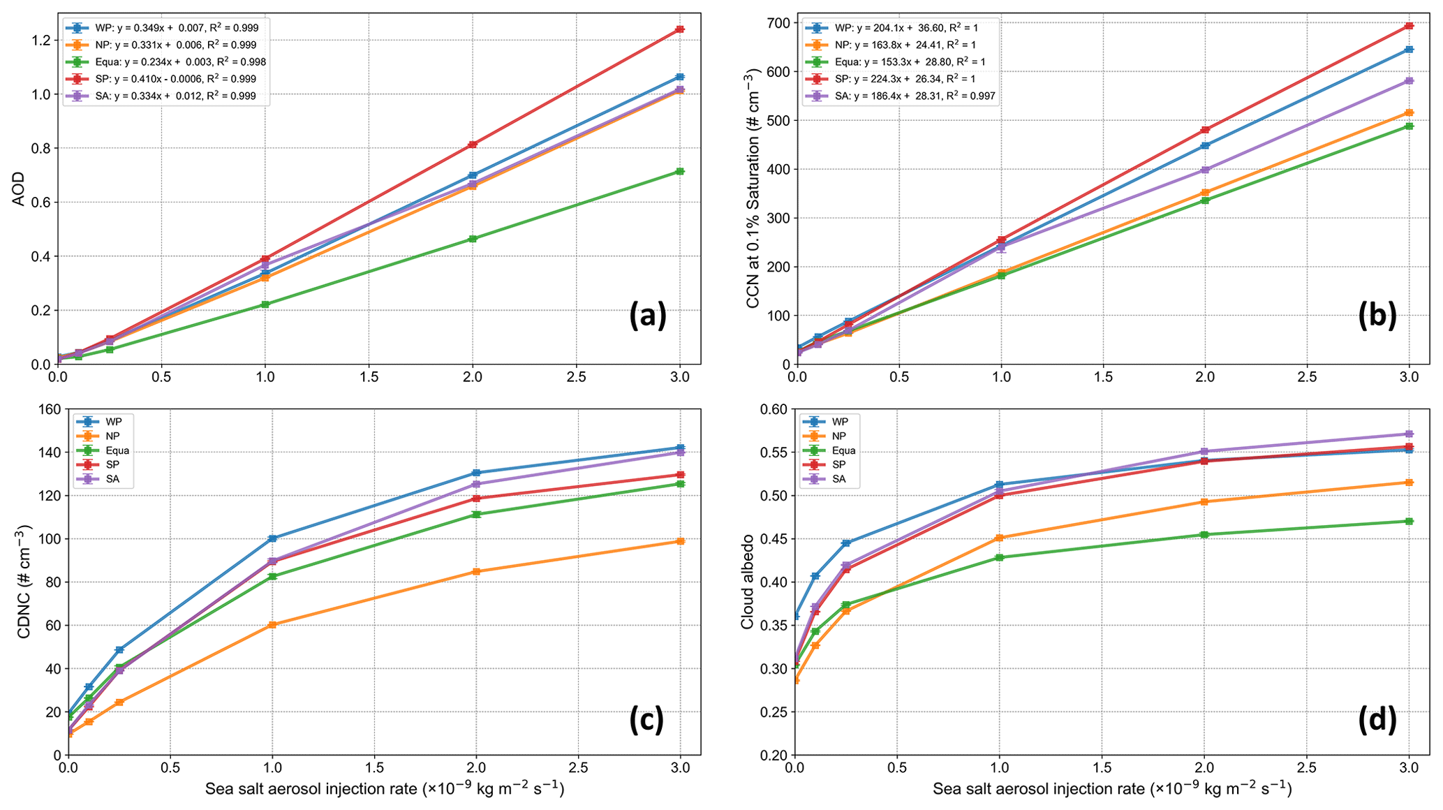
Figure 9 Relationship between changes in the regional mean (a) AOD, (b) CCN, (c) CDNC, and (d) cloud albedo due to uniform injection of sea salt aerosols across the region and the amounts of sea salt aerosols injected. The results for the linear regression of (a) AOD and (b) CCN in the sea salt aerosol injection amounts are given in the legend.

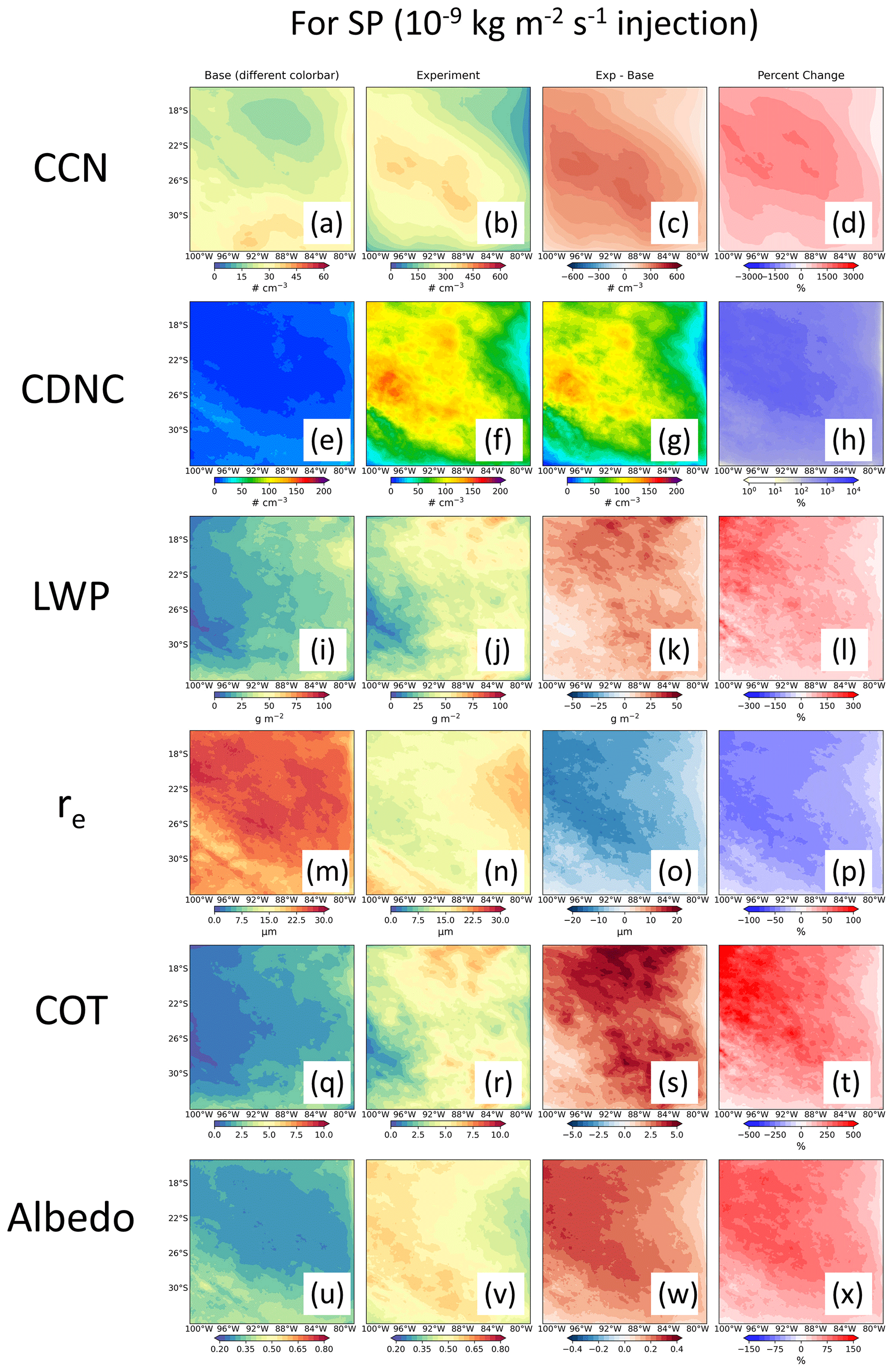
Figure 10 Spatial distribution of liquid cloud property responses after uniform injection of sea salt aerosols totaling 10⁻⁹ kg m⁻² s⁻¹ in the SP region. Results are shown for CCN (S = 0.1 %, cm⁻³), cloud droplet number concentration (cm⁻³), liquid water path (LWP, g m⁻²), cloud effective radius (r_e, µm), cloud optical thickness (COT), and cloud albedo for Base (first column), Exp (second column), and Exp − Base (third column), together with the percentage change in Exp − Base (fourth column).

In the regions with more cloud cover, such as NP, SP, and SA, injected sea salt aerosols significantly increase the cloud fraction (Fig. 2, third column; Table 1), leading to the formation of more clouds or expanding the coverage, vertical thicknesses, and lifetimes of existing clouds (Goddard et al., 2022). Taking the SP region as an example, Fig. 10 demonstrates that uniform injections of 10⁻⁹ kg m⁻² s⁻¹ of sea salt aerosols increase the CDNC significantly. More cloud droplets capture more water vapor, leading to an increase in the LWP. Additionally, the increases in cloud thickness also contribute to the increase in the LWP. The increase in the CDNC decreases the mean r_e by 8.9 µm (∼ −37 %), increases the COT by more than 220 %, and ultimately increases the mean cloud albedo over the region by 0.19 (∼ 64 %). Similarly, injecting sea salt aerosols in the NP and SA regions leads to average cloud albedo increases of 0.17 and 0.20, respectively, while in WP and Equa the increases are 0.15 and 0.13, respectively (Figs. S8–S11). The uniform injection of sea salt aerosols within the sensitive areas results in smaller effects on cloud microphysical properties compared to uniform injections across the entire region, even though the total injection amount within the sensitive areas is the same in both scenarios. This is because, when sea salt aerosols are injected across the entire region, the surrounding sea salt aerosols affect the sensitive areas through transport, resulting in an enhanced cumulative effect on cloud microphysical properties in the sensitive areas. Injecting sea salt aerosol in the sensitive area of the SP-affected clouds in the surrounding region through transport increases the average cloud albedo by 0.032 over the entire region and by 0.12 within the sensitive areas, which is less than the effects of injection across the entire region (Fig. S12). Similarly, injecting sea salt aerosols in the sensitive areas of other ocean regions leads to average cloud albedo increases of 0.015–0.024 across the entire area, with increases of 0.11 in the sensitive areas of the SP and SA regions and increases of 0.090 and 0.10 in WP and Equa, respectively (Figs. S12–S16).

3.5 Drivers of SW_CLD responses

The CRF parameters are used to calculate the effects of changes in cloud cover and cloud albedo on the SW_CLD responses due to the injections of sea salt aerosols. Figure S17 illustrates the increase in the CRF parameter coinciding with the increases in the SW_CLD responses after uniform injection of sea salt aerosols in the five regions (Fig. S5, third row). The CRF${}_{\mathrm{param}}^{\prime }$ calculated using the perturbation method indicates that, in the five ocean regions, CRF${}_{\mathrm{param}}^{\prime }$ is primarily driven by perturbations in cloud albedo (Fig. S18, first column), and it surpasses the changes in cloud fractions and their interactions. Cloud albedo changes explain over 70 % of the CRF${}_{\mathrm{param}}^{\prime }$ in all five regions except Equa (Table 3). The contribution of cloud fraction changes ranges from 13.9 % to 23.7 %, while the interactions between the two factors account for only about 10 % (Fig. S18, second and third columns).

Table 3 Relative effects of cloud fraction and albedo changes on CRF${}_{\mathrm{param}}^{\prime }$ as well as Twomey, LWP, and cloud fraction effects on SW_CLD responses after uniform fixed injection of 10⁻⁹ kg m⁻² s⁻¹ of sea salt aerosols over the five ocean regions.​​​​​​​

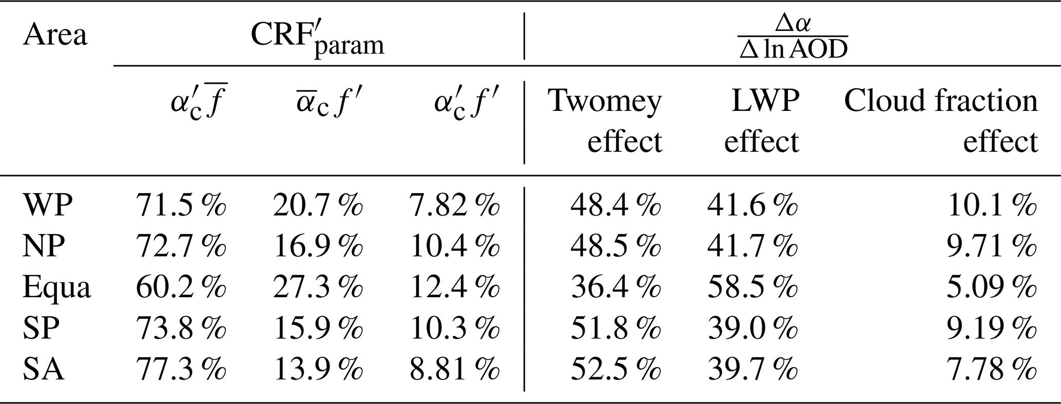
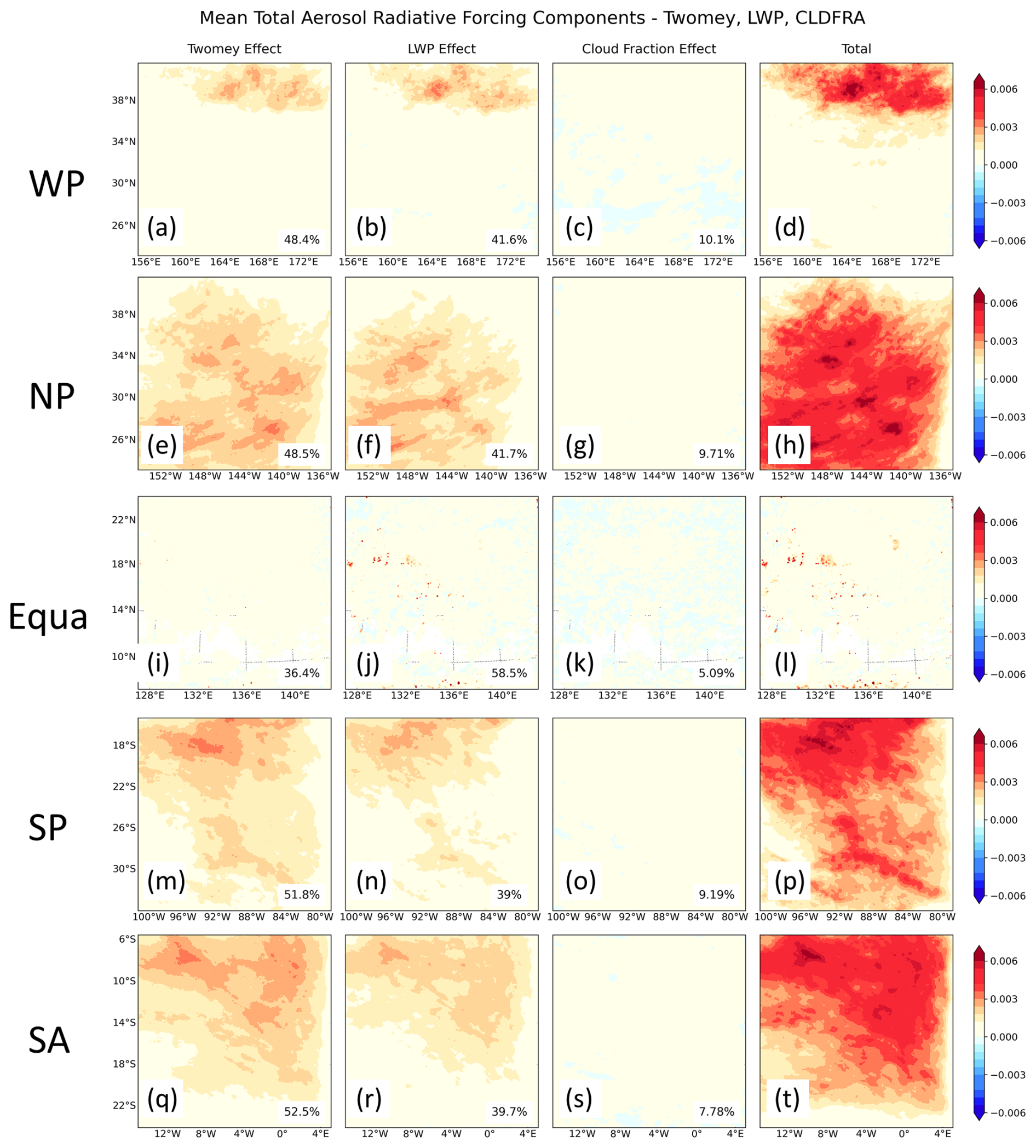
Figure 11 Spatial distribution of cloud property changes in response to SW_CLD radiation after uniform injection of sea salt aerosols in the five regions. The first column is the Twomey effect, the second column is the LWP effect, the third column is the cloud fraction effect, and the fourth column is the cloud susceptibility $\left(\frac{\mathrm{\Delta }\mathit{\alpha }}{\mathrm{\Delta }\ln \mathrm{AOD}}\right)$ to aerosol injection for the sum of the three effects. The percentage contributions of each to the total SW_CLD response over the entire region are shown in the lower-right corner.

Figure 11 evaluates the relative effects of Twomey, LWP, and cloud fractions on the SW_CLD responses after uniformly injecting sea salt aerosols in the five ocean regions. The results indicate that changes in CDNC (Twomey effect) and LWP are the main drivers of the SW_CLD responses, while changes in cloud fraction contribute minimally to the SW_CLD responses. Except for the Equa region, changes in CDNC and LWP account for 48.4 %–52.5 % and 39.0 %–41.7 % of the SW_CLD changes, with cloud fraction changes contributing less than 10.0 % (Fig. 11 and Table 3). The results are similar for injections in sensitive areas, with changes in CDNC and LWP contributing similarly and more than changes in cloud fractions to SW_CLD (Fig. S19). The changes in SW_CLD responses after aerosol injections in the sensitive areas of Equa are mainly contributed by LWP effects (∼ 70 %).

Uniform injections of sea salt aerosols at a rate of 10⁻⁹ kg m⁻² s⁻¹ produced susceptibilities $\left(\frac{\mathrm{\Delta }\mathit{\alpha }}{\mathrm{\Delta }\ln \mathrm{AOD}}\right)$ ranging from 0.00030 to 0.0035 in the five regions, with the corresponding spatial distributions shown in Fig. 11. The NP, SP, and SA regions exhibit cloud responses that are more sensitive to aerosol injections in most of the region, with susceptibilities ranging from 0.0028 to 0.0035. Equa shows the lowest susceptibility, indicating that the system is less responsive to variations in aerosol injections. It is noteworthy that, although the average susceptibility in the WP region is 0.0013, the higher susceptibility values are concentrated north of 35° N, where the average susceptibility is 0.0026, similar to those of the SP region, suggesting that clouds here are more susceptible to aerosol injections. Injecting sea salt aerosols in sensitive areas mostly results in cloud responses that are located outside the sensitive areas (Fig. S19). Injecting sea salt aerosols in the sensitive areas of SP and SA has a greater impact in the northwest. In the sensitive areas of NP, injecting sea salt aerosols has a larger impact in the west. In WP, the injection of sea salt aerosols in the sensitive area does not fully reflect its susceptibility because we choose to calculate the sensitive areas away from the boundary, and the greatest susceptibilities in the WP region happen to be in the northern part of the region near the boundary.

4 Discussions and conclusions

Many studies have discussed the contributions of both direct and indirect effects of MCB. Some studies suggest that MCB relies primarily on indirect effects, as originally conceived, i.e., injecting aerosols to brighten clouds (Jones and Haywood, 2012; Latham et al., 2012). Other studies propose that direct scattering effects of aerosols may be more important (Ahlm et al., 2017; Kravitz et al., 2013; Mahfouz et al., 2023; Niemeier et al., 2013; Partanen et al., 2012). Our results indicate that the importance of both aerosol direct and indirect effects during MCB implementation depends on injection strategies and the choice of injection regions. In the cases of low sea salt aerosol injections or the early stages of MCB implementations, changes in the radiative response are mainly driven by indirect effects, causing clouds to brighten easily. As the injection of sea salt aerosol increases, the radiative effect on clouds saturates and the clouds are difficult to brighten. In contrast, the direct effect continues to increase linearly, leading to a subsequent decrease in the efficiencies of MCB. Partanen et al. (2012) first considered the relative importance of aerosol direct and indirect effects for MCB and preliminarily found the saturated nonlinear phenomenon of indirect effects at a high CDNC, together with the linear relationships between direct effects and injection amounts. Haywood et al. (2023) also found a decrease in MCB efficiency with increasing aerosol injections. Regions initially susceptible to cloud brightening gradually became less susceptible, and aerosol direct radiation effects dominated. Other general circulation model (GCM) studies also found similar results (Alterskjær and Kristjánsson, 2013; Rasch et al., 2024; Stjern et al., 2018).

This study highlights and quantifies these findings in a regional model for the first time, showing the changing trends of direct and indirect effects with injection amounts in the different ocean regions. It provides more detailed cloud composition changes due to sea salt aerosol injection. The model achieves higher droplet nucleation rates at higher resolution due to increased subgrid vertical velocities and higher aerosol concentrations (Ma et al., 2015). The best results are obtained in regions with persistent stratocumulus clouds (e.g., the oceans along the western coast of the continent), where the injected sea salt aerosols work together through both direct and indirect effects. However, in cloud-free or less cloudy regions, MCB implementation can achieve the goal of reflecting more sunlight through the direct scattering effect of aerosols. Considering the uncertainty in the model's resolution of clouds and the fact that, in reality, the cloud distributions are also greatly influenced by the local meteorological conditions, the direct scattering effects of sea salt aerosols on MCB contributions are relatively certain. Therefore, in cloud-free or less cloudy regions, the direct effect of aerosols becomes more important.

In the early stages of Earth system modeling studies, MCB processes were often simulated by presetting CDNC = 375 or 1000 cm⁻³ in the lower regions of the ocean (Jones et al., 2009; Latham et al., 2008; Rasch et al., 2009). However, many follow-up studies have suggested that injections of sea salt aerosols have difficulty in producing a uniform CDNC field due to aerosol dilutions, depositions, and the dependence of the spray rate on wind speed. The CDNC is highly variable spatially, and studies have even reported reductions in CCN and CDNC caused by injections of sea salt aerosols (Alterskjær et al., 2012; Korhonen et al., 2010; Pringle et al., 2012).

In this study, after injecting accumulation-mode sea salt aerosols at a rate of 10⁻⁹ kg m⁻² s⁻¹, the average CDNC concentrations for the five ocean regions range from 60.2 to 100 cm⁻³, and the spatial distributions are uneven (Figs. 10 and S8–S11). Figure 9b indicates that the CCN in the five regions increase linearly (R² = 1) with increasing sea salt aerosol injections, but not all of the CCN are converted into cloud droplets. After doubling the injection amounts, the regional average CDNC is 84.8–130 cm⁻³, with only some grid points exceeding 200 cm⁻³ within the regions. When the injection amounts are increased to 3 × 10⁻⁹ kg m⁻² s⁻¹, the regional average CDNC is 98.8–140 cm⁻³. This implies that injecting more sea salt aerosols at this point does not result in more cloud droplets and that the conversion of CCN into cloud droplets is less efficient, which slows the CDNC growth and tends to saturation (Fig. 9c).

Our findings align with those of Alterskjær et al. (2012), who injected sea salt aerosols at the same rate (10⁻⁹ kg m⁻² s⁻¹) and observed an average CDNC of less than 375 cm⁻³ due to competitive effects and reduced aerosol activation. Notably, however, Wood (2021) found that decreased activation due to competition may be overestimated in the Abdul-Razzak and Ghan activation parameterization used in many GCMs relative to a parcel model. Partanen et al. (2012) used wind-adjusted injections and reported CDNC values of 596–784 cm⁻³, with even higher values (> 1000 cm⁻³) for smaller-sized aerosols, attributing this to overestimations of particle solubility and size. Hill and Ming (2012) increased sea salt aerosol concentrations by a factor of 5, raising the CDNC from 68 to 148 cm⁻³ at 850–925 hPa. It is noteworthy that Hill and Ming (2012) increased all the modes of sea salt aerosols. Many studies have reported that selecting an appropriate injection particle size is crucial for MCB (Andrejczuk et al., 2014; Hoffmann and Feingold, 2021; Partanen et al., 2012), and injecting the Aitken and coarse modes may even lead to a positive forcing with the CDNC decreasing (Alterskjær and Kristjánsson, 2013). However, Wood (2021) argued that particles with a geometric mean dry diameter of 30–60 nm were most effective in brightening cloud layers, and Goddard et al. (2022) similarly found that injecting Aitken-mode sea salt aerosols generated larger radiative flux changes compared to the accumulation mode. There are still considerable discussions about choosing the appropriate aerosol particle sizes during the implementation of MCB, with different models and parameterization schemes providing different recommendations. The sensitivity of MCB to particle size is not considered in this paper and is left to future research.

In this study, the injection of 10⁻⁹ kg m⁻² s⁻¹ of accumulation-mode sea salt aerosols increases cloud albedo in the five ocean regions by 0.13–0.20, with a local maximum of more than 0.3. After doubling the injection amounts, the regional average cloud albedo reaches 0.45–0.55, representing a cloud albedo change of 0.15–0.24 (Fig. 9d). Bower et al. (2006) suggested that, to compensate for the warming associated with doubling atmospheric CO₂ concentrations, a cloud albedo change of 0.16 was needed in three stratocumulus cloud regions (off the western coast of Africa, North America, and South America, representing 3 % of the global cloud cover). The cloud albedo changes produced by the injected aerosols in this study achieved the targets envisioned in previous studies. Wood (2021) proposed seeding Aitken-mode particles in approximately 9 % of the ocean to achieve a corresponding cloud albedo increase of 0.16. It was also suggested that injecting sea salt aerosols in a clean, undisturbed state would produce more brightening (Wood, 2021). Figure 9d confirms this finding, indicating that clouds are more likely to brighten in the early stages of sea salt aerosol injection, and the efficiency of cloud brightening decreases with increasing injection amounts. Goddard et al. (2022), simulating injection of accumulation-mode sea salt aerosols in the central Gulf of Mexico, achieved a simulated cloud albedo change of approximately 0.1 in the main impact region, while switching to Aitken-mode injection resulted in a cloud albedo change of up to 0.35. For the global implementation of MCB, global cloud albedo increases of 0.02 (Bower et al., 2006), 0.062 (Latham et al., 2008), and 0.074 (Lenton and Vaughan, 2009) were estimated.

The contributions of the changes in cloud fractions to the SW_CLD responses in this study are small, which is consistent with the results of Goddard et al. (2022). However, many observational studies indicate that the contribution of the cloud fractions to the shortwave radiative forcing should be similar to those of the CDNC and LWP (Chen et al., 2014; Rosenfeld et al., 2019). Goddard et al. (2022) believe that this is due to the fact that the regional atmosphere was wetter during the simulation periods and that the relative contributions of changes in the cloud fraction to the SW_CLD response will be expected to increase in drier months. Three of the five ocean regions in this study, i.e., SA, SP, and NP, are much drier and more stable than the Gulf of Mexico simulated by Goddard et al. (2022) (Fig. S20). Furthermore, when we switched to conducting the experiments again in the dry months of the same year, the contribution of the cloud fraction to SW_CLD did not change much, remaining at ∼ 10 %. We believe that this difference might be due to the parameterization scheme or resolution of the model. Liu et al. (2020) performed simulations with the WRF–Chem model and found that the cloud fraction susceptibilities to aerosols in the Morrison scheme and Lin scheme were only about half of those observed by the Moderate Resolution Imaging Spectroradiometer (MODIS). The neglected subgrid clouds in the 12 km resolution simulations might lead to an underestimation of the radiative effects of clouds (Yu et al., 2014). In addition, cloud fractions are more commonly underestimated in the model (Glotfelty et al., 2019), and using an updated parameterization scheme that accounts for subgrid condensation might improve the model's ability to resolve clouds (Zhao et al., 2023). The high spatial variabilities of cloud radiative effects emphasize the need for improved resolution in future model studies of cloud–aerosol interactions. The effects of a finer resolution and more parameterization schemes on aerosol–cloud interactions still need to be verified. Considering the modeling difficulties in accurately capturing the effects of cloud fractions on radiation, the actual effects of MCB may be underestimated.

This study provides quantifiable data on cloud and radiation changes for the implementation of MCB over the five ocean regions as well as an optimization scheme for the injection strategy of adjusting the injection amounts and selecting sensitive areas. It is noteworthy that different parameterization schemes, models, and resolutions can influence the results, especially the cloud feedback on the injected sea salt aerosols, which is a major reason for the discrepancies between the models (Stjern et al., 2018). In Earth system model studies, there has been a rich discussion on the climate and ecological impacts of the MCB with the same framework as the Geoengineering Model Intercomparison Project (GeoMIP) (Rasch et al., 2024). However, there is still a lack of a unified framework for mid-scale MCB research.