Air-pollution-satellite-based CO₂ emission inversion: system evaluation, sensitivity analysis, and future research direction

Simultaneous monitoring of greenhouse gases and air pollutant emissions is crucial for combating global warming and air pollution. We previously established an air-pollution-satellite-based carbon dioxide (CO₂) emission inversion system, successfully capturing CO₂ and nitrogen oxide (NO_x) emission fluctuations amid socioeconomic changes. However, the system's robustness and weaknesses have not yet been fully evaluated. Here, we conduct a comprehensive sensitivity analysis with 31 tests on various factors including prior emissions, model resolution, satellite constraint, and inversion system configuration to assess the vulnerability of emission estimates across temporal, sectoral, and spatial dimensions. The relative change (RC) between these tests and base inversion reflects the different configurations' impact on inferred emissions, with 1 standard deviation (1σ) of RC indicating consistency. Although estimates show increased sensitivity to tested factors at finer scales, the system demonstrates notable robustness, especially for annual national total NO_x and CO₂ emissions across most tests (RC < 4.0 %). Spatiotemporally diverse changes in parameters tend to yield inconsistent impacts (1σ ≥ 4 %) on estimates and vice versa (1σ < 4 %). The model resolution, satellite constraint, and NO_x emission factors emerge as the major influential factors, underscoring their priority for further optimization. Taking daily national total CO₂ emissions as an example, the $\stackrel{\mathrm{‾}}{\text{RC}}$ ± 1σ they incur can reach −1.2 ± 6.0 %, 1.3 ± 3.9 %, and 10.7 ± 0.7 %, respectively. This study reveals the robustness and areas for improvement in our air-pollution-satellite-based CO₂ emission inversion system, offering opportunities to enhance the reliability of CO₂ emission monitoring in the future.

1 Introduction

The knowledge of emissions, i.e., how much, where, and by what activity pollutants are released into the atmosphere, lays the foundation for understanding the changes in atmospheric compositions and managing emissions toward climate and air quality targets (Meinshausen et al., 2022; Li et al., 2022; Zhang et al., 2019). Anthropogenic emissions are strongly modulated by socioeconomic events (e.g., holidays, economic recession, and recovery). Therefore, it is essential to monitor emissions timely to interpret atmospheric species concentrations (Shan et al., 2021; Le Quéré et al., 2021; Guevara et al., 2023). Currently, numerous nations, particularly those within the Global South (i.e., China), grapple with the dual imperatives of mitigating air pollution and addressing climate change challenges. To effectively navigate these intertwined challenges in a harmonized and resource-efficient manner, the development of a system capable of disentangling variations in emissions and their driving factors for greenhouse gases and air pollutants is indispensable (Ke et al., 2023).

Recently, a discernible trend is emerging towards inferring anthropogenic carbon dioxide (CO₂) emissions from well-observed and co-emitted air pollutants (i.e., nitrogen dioxide, NO₂) given their co-emission characteristics in time and space (Wren et al., 2023; Yang et al., 2023; F. Liu et al., 2020a; Reuter et al., 2019). NO₂ forms rapidly after NO is emitted from sources and is also the primary nitrogen oxide detectable by most satellites (Ye et al., 2016). This makes NO₂ a reliable and widely adopted proxy in nitrogen oxide (${\mathrm{NO}}_x={\mathrm{NO}}_{\mathrm{2}}+\mathrm{NO}$) emission inversions. However, the co-emission of NO_x and CO₂ does not imply synchronized trends in their emissions, as the CO₂-to-NO_x emission ratios and activity trends vary across different sectors (Li and Zheng, 2024). The introduction of NO₂ in the CO₂ emission estimation presents several distinct advantages. NO₂ has a short lifetime of several hours, rendering its source-contributing plumes readily detectable via remote sensing techniques (Goldberg et al., 2019). This short lifespan of NO₂ facilitates mass-balance approaches for estimating NO_x emissions, which rely on the assumption of a linear relationship between NO₂ columns and local NO_x emissions (Cooper et al., 2017; Mun et al., 2023; Martin et al., 2003). In contrast, the longevity of CO₂, spanning hundreds of years, combined with its elevated background concentration reaching hundreds of parts per million (ppm), obscures the detection of local source-triggered concentration enhancements (i.e., several ppm) (Nassar et al., 2017; Reuter et al., 2019). Moreover, remote sensing technologies for NO₂ remain generally more mature, as indicated by the broader coverage and improved signal-to-noise ratio in column concentration observation (MacDonald et al., 2023; Cooper et al., 2022). Recent advancements in CO₂ satellite technology are promising, such as Orbiting Carbon Observatory-3 (OCO-3), which can generate CO₂ maps with a resolution of up to 1.6 km × 2.2 km and monitor CO₂ columns at different times throughout the daytime to elucidate diurnal emission patterns (Taylor et al., 2023), while its spatial coverage may not be sufficient for large-area inversions at high temporal resolution. The synergistic quantification of CO₂ and NO_x emissions has gained substantial attention, not to mention that it could provide valuable guidance for a joint effort in monitoring and mitigating air pollutants and carbon emissions concurrently (Miyazaki and Bowman, 2023).

We have developed an air-pollution-satellite-based CO₂ emission inversion system, which is capable of concurrently estimating the 10 d moving average of sector-specific anthropogenic NO_x and CO₂ emissions by integrating top-down and bottom-up methods. This integrated methodology has proven effective in capturing emission fluctuations, particularly during the coronavirus disease 2019 (COVID-19) pandemic (Zheng et al., 2020; Li et al., 2023). While previous sensitivity tests have suggested a certain level of accuracy, the system has not yet undergone a comprehensive evaluation to thoroughly assess its robustness and weaknesses and thereby clearly imply its future developmental trajectory. To bridge this gap, we undertake an extensive sensitivity analysis with 31 tests using the 2022 anthropogenic NO_x and CO₂ emission estimation as a case study. This study investigates how emission outcomes respond to a variety of sensitivity assessments across temporal, sectoral, and spatial dimensions. This study aims to diagnose and rank the uncertainty sources, providing insights to prioritize improvements of this inversion system in the future.

2 Materials and methods

Our air-pollution-satellite-based CO₂ emission inversion system has been elucidated in our previous studies (Zheng et al., 2020; Li et al., 2023). In essence, this system integrates top-down and bottom-up data streams to infer the 10 d moving average of anthropogenic NO_x and CO₂ emissions by sector in China based on the mass-balance approach (Cooper et al., 2017). Comprising three key components, the system involves the bottom-up inference of prior emissions for NO_x and CO₂ with a sectoral profile, the top-down estimation of total NO_x emissions constrained by satellite observation, and the integration of both sources to derive satellite-constrained NO_x and CO₂ emissions by sector (Fig. S1 in the Supplement). Each of these processes could introduce uncertainties in the final emission estimates. To assess the potential uncertainties, we establish a baseline (base) for emissions computed using our conventional settings (Li et al., 2023; Zheng et al., 2020) and further investigate sensitivity tests to characterize the impacts of the different configurations on final estimates.

2.1 Inversion methodology and base inversion

We use the base inversion as a case to provide a detailed explanation of this inversion system. In the base inversion, we adhered to the same parameters and configurations outlined in previous studies for estimating the 10 d moving average of anthropogenic NO_x and CO₂ emissions by sector in 2022 (Table 1) (Li et al., 2023; Zheng et al., 2020). Succinctly, we first updated sectoral NO_x and CO₂ emissions from the Multi-resolution Emission Inventory for China (MEIC) (Zheng et al., 2018) through the bottom-up process. This involved utilizing indicators including industrial production, thermal power generation, freight turnover, and population-weighted heating degree days as proxies for changes in industry, power, transport, and residential activity levels (details are shown in Sect. S1 and Table S1 in the Supplement). Notably, to reconcile the resolution between the prior emissions and the model, we aggregated the original MEIC emissions from a resolution of 0.25° × 0.25° (Fig. S2 in the Supplement) to 0.5° × 0.625°. Secondly, we inferred the total anthropogenic NO_x emissions constrained by TROPOspheric Monitoring Instrument (TROPOMI) NO₂ retrievals (v2.4) (van Geffen et al., 2022) (Eq. 1). A critical step in this process was establishing a linear relationship between NO₂ tropospheric vertical column densities (TVCDs) and anthropogenic NO_x emissions under the mass-balance assumption (Eq. 2) through the GEOS-Chem (GC) simulation (v12.3.0, https://geoschem.github.io/, last access: 1 October 2019) at a horizontal resolution of 0.5° × 0.625°. Our analysis focused on the grids where anthropogenic emissions prevail (F. Liu et al., 2020b), characterized by a 10 d moving average of NO₂ TVCDs exceeding 1×10¹⁵ molec. cm⁻².

$$\begin{array}{}\text{(1)}& \begin{array}{rl}{E}_{t,i,\mathrm{TROPOMI},y}& =\left(\mathrm{1}+{\mathit{\beta }}_{t,i}{\left({\displaystyle \frac{\mathrm{\Delta }\mathrm{\Omega }}{\mathrm{\Omega }}}\right)}_{t,i,\mathrm{anth},y}\right)\\ & \times E_{t,i,\mathrm{bottom}\text{-}\mathrm{up},\mathrm{2019}}\end{array}\end{array}$$

$$\begin{array}{}\text{(2)}& \begin{array}{rl}{\mathit{\beta }}_{t,i}& ={\displaystyle \frac{\mathrm{\Delta }{E}_{t,i,\mathrm{bottom}\text{-}\mathrm{up},\mathrm{2019}}}{E_{t,i,\mathrm{bottom}\text{-}\mathrm{up},\mathrm{2019}}}}\\ & ÷{\displaystyle \frac{{\mathrm{\Omega }}_{t,i,-\mathrm{40}\mathit{\%}\mathrm{emi},\mathrm{2019}}-{\mathrm{\Omega }}_{t,i,\mathrm{base},\mathrm{2019}}}{{\mathrm{\Omega }}_{t,i,\mathrm{base},\mathrm{2019}}}}\end{array}\end{array}$$

$$\begin{array}{}\text{(3)}& {\left({\displaystyle \frac{\mathrm{\Delta }\mathrm{\Omega }}{\mathrm{\Omega }}}\right)}_{t,i,\mathrm{anth},y}={\displaystyle \frac{{\mathrm{\Omega }}_{t,i,\mathrm{sate},y}}{{\mathrm{\Omega }}_{t,i,\mathrm{sate},\mathrm{2019}}}}-{\displaystyle \frac{{\mathrm{\Omega }}_{t,i,\mathrm{simu}\mathit{\_}\mathrm{fixemis},y}}{{\mathrm{\Omega }}_{t,i,\mathrm{simu},\mathrm{2019}}}},\end{array}$$

where t, i, and y represent the 10 d window, model grid cell (i.e., 0.5° × 0.625°), and target year 2022, respectively. $E_{t,i,\mathrm{TROPOMI},y}$ is the anthropogenic total NO_x emissions constrained by TROPOMI NO₂ TVCDs. $E_{t,i,\mathrm{bottom}\text{-}\mathrm{up},\mathrm{2019}}$ is the anthropogenic NO_x emissions in 2019 from the MEIC. β_t,i is a unitless factor relating the changes in NO₂ TVCDs to anthropogenic NO_x emissions (Lamsal et al., 2011). $\mathrm{\Delta }{E}_{t,i,\mathrm{bottom}\text{-}\mathrm{up},\mathrm{2019}}/E_{t,i,\mathrm{bottom}\text{-}\mathrm{up},\mathrm{2019}}$ represents the implemented 40 % reduction in anthropogenic NO_x emissions over China. The 40 % reduction was selected after a series of sensitivity tests, which demonstrated that this perturbation level exerts a limited impact on the β estimates (Zheng et al., 2020). ${\mathrm{\Omega }}_{t,i,-\mathrm{40}\mathit{\%}\mathrm{emi},\mathrm{2019}}$ and ${\mathrm{\Omega }}_{t,i,\mathrm{base},\mathrm{2019}}$ are GEOS-Chem-simulated NO₂ TVCDs at the TROPOMI overpass time in 2019 with a 40 % emission reduction and without any emission reduction, respectively. ($\mathrm{\Delta }\mathrm{\Omega }/\mathrm{\Omega }{)}_{t,i,\mathrm{anth},y}$ refers to the relative changes in NO₂ TVCDs due to anthropogenic NO_x emission changes between 2019 and 2022. ${\mathrm{\Omega }}_{t,i,\mathrm{sate},y}/{\mathrm{\Omega }}_{t,i,\mathrm{sate},\mathrm{2019}}$ indicates the relative differences in TROPOMI NO₂ TVCDs between 2019 and 2022, and ${\mathrm{\Omega }}_{t,i,\mathrm{simu}\mathrm{\_}\mathrm{fixemis},y}/{\mathrm{\Omega }}_{t,i,\mathrm{simu},\mathrm{2019}}$ represents the relative changes in NO₂ TVCDs caused by inter-annual meteorological variation, which are derived from GEOS-Chem simulations with the fixed 2019 emissions and meteorological field in the target year.

Thirdly, we integrated the bottom-up and top-down data flows to yield TROPOMI-constrained sectoral NO_x emissions. Assuming that each grid's emission variability was primarily driven by its dominant source sectors (contributing over 50 %), we utilized the discrepancy between the bottom-up and top-down estimates in grid cells dominated by a particular sector to derive sector-specific scaling factors, which were subsequently applied to correct the bottom-up sectoral NO_x emissions (Eq. 4). For grids without a sector contributing over 50 %, we excluded them from sectoral scaling factor calculations, instead applying scaling factors derived from grids meeting this criterion. The number of these grids accounts for less than 20 % of total grids, making their impact negligible. Following this adjustment, we rescaled the corrected bottom-up emissions to ensure alignment with the TROPOMI-constrained total emissions. The overall sectoral correction factors mainly range from 0.5 to 1.5 (Fig. S3).

$$\begin{array}{}\text{(4)}& {\mathrm{\text{scale factor}}}_{t,s,y}=\mathrm{1}+{\displaystyle \frac{{\sum }_i\left(E_{t,i,\mathrm{sate},y}^s-E_{t,i,\mathrm{bottom}\text{-}\mathrm{up},y}^s\right)}{{\sum }_i{E}_{t,i,\mathrm{bottom}\text{-}\mathrm{up},y}^s}},\end{array}$$

where t, s, i, and y represent the 10 d window, sector, grid cell (i.e., 0.5° × 0.625°), and year 2022, respectively. $E_{t,i,\mathrm{sate},y}^s$ and $E_{t,i,\mathrm{bottom}\text{-}\mathrm{up},y}^s$ are TROPOMI-constrained and bottom-up-estimated NO_x emissions on grid cell i with dominated source sector s, respectively. The scale factor ${}_{t,s,y}$ is the scaling factor used to correct the bottom-up-estimated NO_x emissions from sectors in time t in year y.

Finally, we converted the sectoral NO_x emissions to corresponding CO₂ emissions with the CO₂-to-NO_x emission ratios derived from the bottom-up process (Eq. 5). The CO₂-to-NO_x emission ratios in 2022 are updated by reducing NO_x emission factors (EFs) while keeping CO₂ EFs unchanged based on the 2019 MEIC. The default assumption that the reduction rate halves annually is due to the limited potential for further reductions. In contrast, the CO₂ EFs are assumed to remain unchanged, as they are primarily determined by fuel type and combustion conditions (Cheng et al., 2021) (details shown in Sect. S2).

$$\begin{array}{}\text{(5)}& \begin{array}{rl}& C_{s,t,i,\mathrm{TROPOMI},y}=E_{s,t,i,\mathrm{TROPOMI},y}\\ & \times {\displaystyle \frac{{\text{EF}}_{{\mathrm{CO}}_{\mathrm{2}}s,i,\mathrm{bottom}\text{-}\mathrm{up},\mathrm{2019}}}{{\text{EF}}_{{\mathrm{NO}}_{x}s,i,\mathrm{bottom}\text{-}\mathrm{up},\mathrm{2019}}\times \left(\mathrm{1}-r{\mathrm{NO}}_{xs,i,y}\right)}},\end{array}\end{array}$$

where $C_{s,t,i,\mathrm{TROPOMI},y}$ and $E_{s,t,i,\mathrm{TROPOMI},y}$ are CO₂ and NO_x emissions from sector s. EF${}_{{\mathrm{CO}}_{\mathrm{2}}s,i,\mathrm{bottom}\text{-}\mathrm{up},\mathrm{2019}}$ and EF${}_{{\mathrm{NO}}_{x}s,i,\mathrm{bottom}\text{-}\mathrm{up},\mathrm{2019}}$ are the sectoral EFs of CO₂ and NO_x in 2019 derived from the MEIC emission model. rNO${}_{{}_{x}s,i,y}$ is the reduction ratio in NO_x EFs by sector from 2019 to 2022 derived from the bottom-up estimation.

We approximate the annual NO_x and CO₂ emissions as the sum of the 10 d moving average of NO_x and CO₂ emissions in 2022 with a vacancy in the first and last 5 d. This approximation, however, does not impact our analysis, as our primary objective is to identify potential sources of uncertainty within the system and thereby highlight areas for future improvement.

Table 1 Configurations of base inversion.

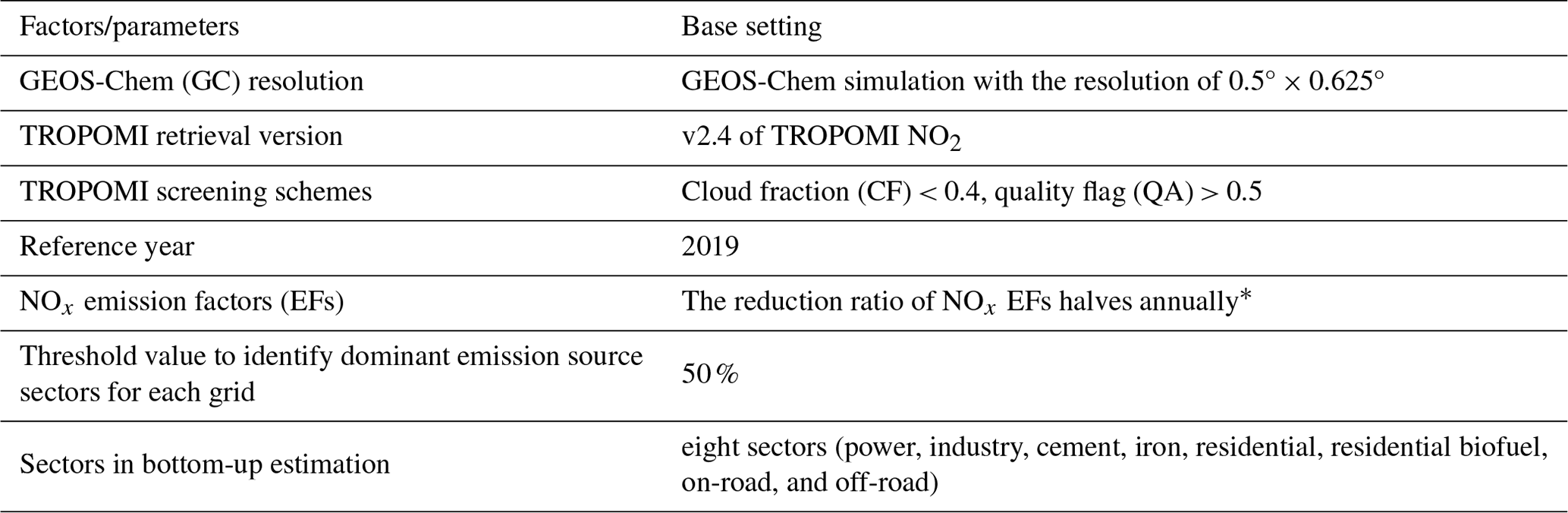
^* Each year's reduction rate for NO_x EFs is set to decrease by half compared to the previous year. For example, if the reduction of NO_x EFs from 2019 to 2020 were 4 %, the reduction from 2020 to 2021 would be set at 2 %.

2.2 Sensitivity settings

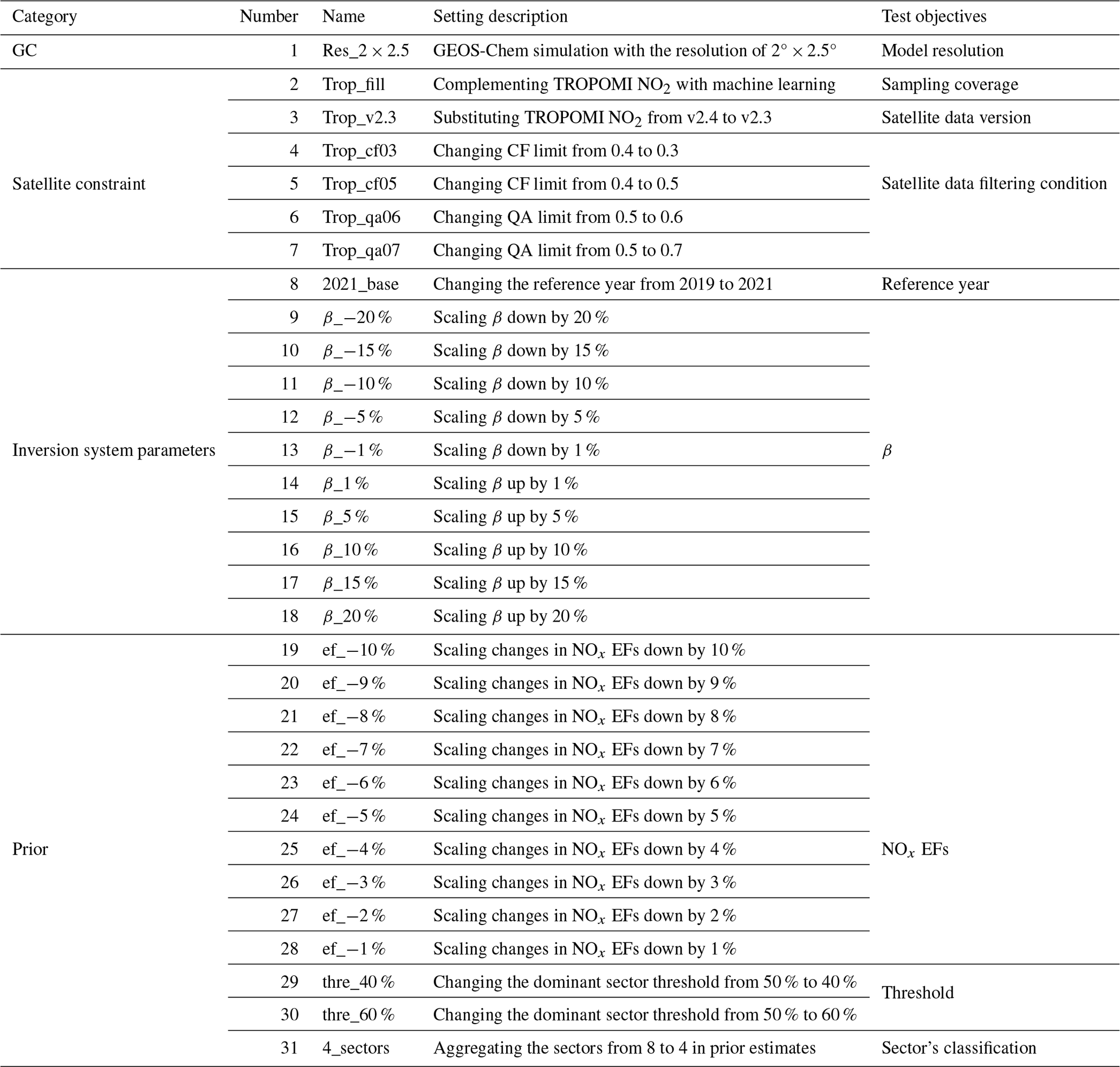
The sensitivity inversion experiments comprise 31 tests designed to provide a comprehensive evaluation of the system. To facilitate a clearer discussion of their impacts, we categorized these tests into four classes based on their roles within the system: prior information, GEOS-Chem model resolution, satellite observational constraints, and inversion system parameters (Fig. 1 and Table 2). Each test is conducted as a controlled experiment, where only one parameter is altered, while the rest remain the same as their base inversion setting. The rationale behind the settings and their design will be elaborated on in the following sections.

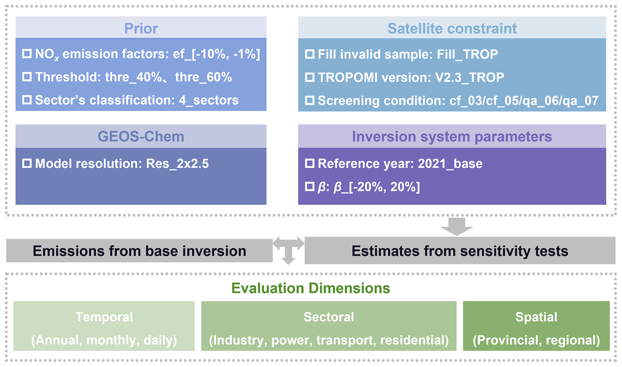
Figure 1 Overview of the sensitivity inversion tests in this study. Details on the processes and settings are presented in Fig. S1 and Table 2.

Table 2 Settings of 31 sensitivity inversion tests.

2.2.1 Modifying prior emission estimates

The prior provides the sectoral profile for subsequent emission attribution. We conducted a comprehensive examination of associated parameters when updating the prior from the 2019 MEIC (0.5° × 0.625°), including NO_x EFs influencing the conversion of NO_x to CO₂ emissions by sector, threshold value defining the dominant sector for each grid, and sector classification. For NO_x EF settings, we devised a 10-level gradient ranging from −10 % to −1 % (referred to as ef_[−10 %, −1 %]). Regarding the threshold value, we varied it from 50 % to 40 % and to 60 % (referred to as thre_40 % and thre_60 %), respectively. For sector classification, the original prior NO_x and CO₂ emissions were updated based on eight sectors in the bottom-up process: power, industry, cement, iron, residential, residential biofuel, on-road, and off-road. This detailed sectoral structure facilitates relatively detailed bottom-up estimations with specific sectoral activity levels. These eight sectors were then aggregated into four categories: power, industry (sum of original industry, cement, and iron), residential (sum of original residential and residential biofuel), and transport (sum of original on-road and off-road) when allocating TROPOMI-constrained total NO_x emissions into sectors. Here, this sector consolidation, specifically implemented before the bottom-up estimation (4_sectors), was designed to evaluate the influence of sector classification on the inversion results.

2.2.2 Employing coarser model resolution

The model resolution of the GEOS-Chem simulation inherently shapes the localized relationship between NO₂ TVCDs and NO_x emissions established in the top-down process. Finer resolution is advantageous for establishing localized connections between air pollutant emissions and atmospheric concentrations, as well as the attribution of sectoral emissions. However, excessively fine resolution is not applicable due to the inter-grid transport when employing the mass-balance method (Turner et al., 2012). To explore the impact of resolution on emission estimates, we performed an inversion experiment with simulations at a coarser resolution of 2° × 2.5° (Res_2 × 2.5).

2.2.3 Changing satellite observational constraints

The TROPOMI NO₂ retrievals serve as a constraint in the top-down NO_x emission estimation. We conducted experiments on the TROPOMI NO₂ retrievals through three distinct approaches. Firstly, we used XGBoost (eXtreme Gradient Boosting) to fill the invalid satellite retrievals in v2.4 TROPOMI (Trop_fill) by establishing relationships between TROPOMI NO₂ TVCDs and meteorological variables, as well as GEOS-Chem-simulated NO₂ TVCDs (modeled_NO₂ in Eq. 6) (Wei et al., 2022). The meteorological variables were derived from the European Centre for Medium-Range Weather Forecasts (ECMWF) ERA5 dataset (Hersbach et al., 2020), including boundary layer height (BLH), surface pressure (SP), temperature (TEM), dew-point temperature (DT), 10 m u component (WU), 10 m v component of winds (WV), total precipitation (TP), evaporation (EP), downward UV radiation at the surface (surUV), and mean surface downward UV radiation flux (downUV). In the XGBoost process, we trained the relationship for daily NO₂ TVCDs throughout the year grid by grid, with 80 % of the data used as the training set and 20 % as the test set.

$$\begin{array}{}\text{(6)}& \begin{array}{rl}& {\text{TROPOMI\_NO}}_{\mathrm{2}}\sim f_{\mathrm{XGBoost}}\\ & ({\text{modeled\_NO}}_{\mathrm{2}},\text{BLH},\text{SP},\text{TEM},\text{DT},\text{WU},\text{WV},\text{TP},\\ & \text{EP},\text{surUV},\text{downUV})\end{array}\end{array}$$

The comparison of NO₂ TVCDs before and after data filling revealed minimal impact from the original missing data (Fig. S4). This is attributed to our system's utilization of a 10 d moving average of NO₂ TVCDs, which effectively mitigates the influence of missing data at the grid scale.

Secondly, we evaluated the impact of different versions of TROPOMI NO₂ retrievals by substituting the v2.4 TROPOMI data with the older v2.3 TROPOMI NO₂ columns (Trop_v2.3). Updates in TROPOMI data products generally help address the low bias of NO₂ concentrations, particularly in heavily polluted regions (Lange et al., 2023; van Geffen et al., 2022). Thirdly, we adjusted the satellite data screening protocols to investigate the uncertainties associated with satellite observations in emission estimates, which involved varying the cloud fraction (CF) limit to 0.3 (Trop_cf03) or 0.5 (Trop_cf05) and modifying the quality flag (QA) limit to 0.6 (Trop_qa06) or 0.7 (Trop_qa07), respectively. CF and QA serve as crucial parameters in screening applicable NO₂ TVCDs, representing primary sources of uncertainty in satellite observations (van Geffen et al., 2022; Lange et al., 2023).

2.2.4 Tests on inversion system parameters

In previous studies, the reference year for updating emissions for target years was 2019. Here, we modified the reference year to 2021 (2021_base) to assess its impact. The parameter β represents the localized relationship between changes in NO₂ TVCDs and changes in anthropogenic NO_x emissions (Eq. 2), determining the transition from observed changes in NO₂ TVCDs to changes in anthropogenic NO_x emissions in the top-down process. To explore potential nonlinear responses in the estimated results to this parameter, we devised a 10-level gradient for β, ranging from −20 % to 20 % (referred to as β_[−20 %, 20 %]).

2.3 Evaluation of different configurations' impact

The sensitivity analysis of the NO_x and CO₂ emissions estimated by our inversion system has illuminated potential sources of uncertainty and the magnitude of their impacts. To quantify the influence of sensitivity tests on emission estimates, we calculated the relative change (RC) between emissions estimated under different tests and the base inversion and 1 standard deviation (1σ) of RC to evaluate the consistency of their impact across temporal, sectoral, and spatial scales (details shown in Table 3). It is noteworthy that on the annual national total emission scale (maximization of all three dimensions), the value of 1σ equals 0.0 %.

Table 3 Calculation of RC and 1σ across different dimensions.

In this context, a condition where 1σ is below 4.0 % is deemed a consistent impact on emission outcomes within certain dimensions (the determination of 4.0 % shown in Fig. S5). Conversely, when 1σ exceeds or equals 4.0 %, it is indicative of an inconsistent impact. For instance, a daily-scale σ_t value of 6.2 % in the Res_2 × 2.5 test (Fig. S6) suggests that the model resolution exerts a temporally inconsistent influence on daily emission estimates, whereas a daily-scale σ_t = 0.0 % under ef_−10 % indicates temporal consistency in its influence. These principles extend to other dimensions (i.e., sectoral and spatial). Factors whose sensitivity tests yield large and inconsistent RC across finer time, sector, or region scales tend to introduce high uncertainty and become a priority for future optimization. Conversely, small and consistent RC suggests sources with low uncertainty and a higher level of robustness in the system to those particular factors.

3 Results

3.1 Overview of the emission responses to sensitivity tests

For a comprehensive understanding of emission sensitivity across various dimensions, we compute the sum of absolute average RC and 1σ (i.e., $\left|\stackrel{\mathrm{‾}}{\text{RC}}\right|+\mathrm{1}\mathit{\sigma }$) to delineate potential most likely uncertainties associated with tested factors across spatial, temporal, and sectoral scales (Fig. 2). The impacts of these tests on emissions are comparable between NO_x and CO₂, except for the NO_x EF tests (first column in Fig. 2), which distinctly influence NO_x and CO₂ emissions. CO₂ emissions display high sensitivity to NO_x EFs across all dimensions compared to NO_x emissions, except in the residential sector where NO_x emissions are more responsive while CO₂ emissions are not. For instance, ef_−10 % (maximum reduction in NO_x EF tests) incurs a $\left|\stackrel{\mathrm{‾}}{\text{RC}}\right|+\mathrm{1}\mathit{\sigma }$ of 10.7 % in annual national CO₂ emissions, with no corresponding impact on NO_x emissions. The relationship between annual national CO₂ emissions and NO_x EFs exhibits linearity (Fig. S7), remaining within a 4.0 % range if NO_x EF reductions are kept below 4.0 % (i.e., ef_[−4 %, −1 %]). In contrast, daily residential emissions show a $\left|\stackrel{\mathrm{‾}}{\text{RC}}\right|$ of only 1.0 % in CO₂ but up to 9.1 % in NO_x emissions under the ef_−10 % test.

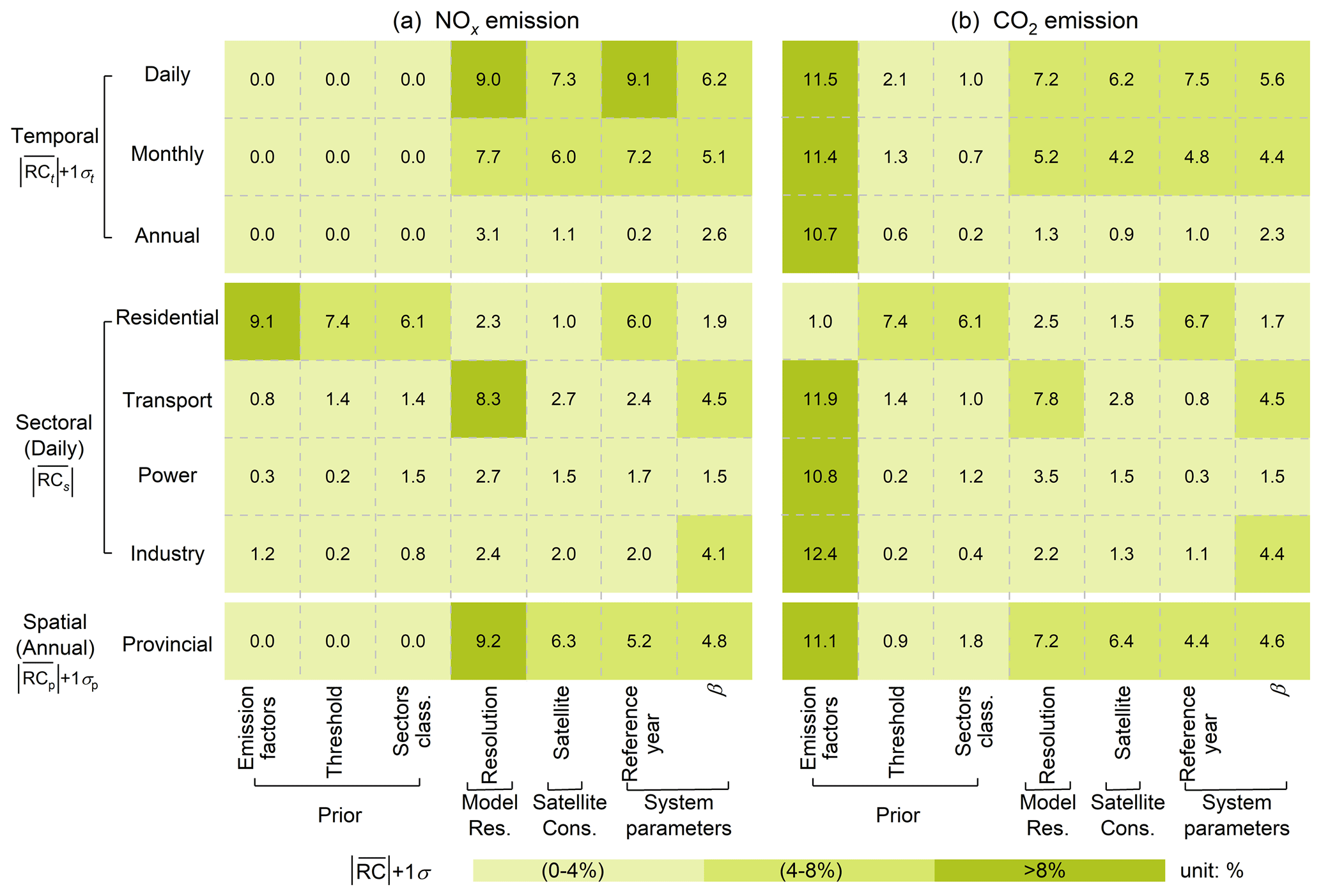
Figure 2 An overview of sensitivity inversion tests' impacts on (a) NO_x and (b) CO₂ emissions. The color blocks in this figure represent the sum of absolute average RC and 1σ (i.e., $\left|\stackrel{\mathrm{‾}}{\text{RC}}\right|+\mathrm{1}\mathit{\sigma }$), which reflect the extent of the corresponding tests' impacts. The numbers within each grid represent the maximum value of $\left|\stackrel{\mathrm{‾}}{\text{RC}}\right|+\mathrm{1}\mathit{\sigma }$ under tests on corresponding factors. For example, the $\left|\stackrel{\mathrm{‾}}{\text{RC}}\right|+\mathrm{1}\mathit{\sigma }$ noted in the emission factors column refers to ef_−10 %. It is noteworthy that the sectoral dimensions in this figure display their absolute average RC on the daily scale, with their corresponding 1σ shown separately in Fig. S6.

The remaining sensitivity tests, excluding the NO_x EFs, demonstrate comparable influences on both NO_x and CO₂ emissions. Among all dimensions examined, the annual national total NO_x and CO₂ emissions emerge as robust results, with a $\left|\stackrel{\mathrm{‾}}{\text{RC}}\right|+\mathrm{1}\mathit{\sigma }$ of no more than 4.0 % across tests. At a finer temporal scale (i.e., daily basis), the impacts of model resolution, reference year, and satellite constraint on estimated emissions are amplified, with their $\left|\stackrel{\mathrm{‾}}{\text{RC}}\right|+\mathrm{1}\mathit{\sigma }$ tripling compared to the annual scale. This amplification primarily arises from the increased 1σ on the daily scale (Fig. S6), indicating the substantial impact of these factors on daily emission estimates. At a finer spatial scale, provincial emissions are vulnerable to changes in model resolution, reference year, and satellite constraint due to their impacts' inconsistency in space (Fig. S6). Concerning sectoral emissions, industry and power sector emissions exhibit robustness, whereas transport and residential emissions present vulnerabilities to model resolution and dominant sector threshold values, respectively. In the following sections, we elaborate on the impacts of all sensitivity tests on NO_x and CO₂ emissions from temporal, sectoral, and spatial perspectives. To clarify the RC across different dimensions, we adopt RC_t, RC_s, and RC${}_{\mathrm{p}/\mathrm{r}}$ to signify RC in temporal, sectoral, and spatial contexts, respectively.

3.2 Emission sensitivity at different temporal scales

To exclusively examine emission sensitivities in the temporal dimension, this section focuses on the variation of national total emissions in each test. Tests influencing both NO_x and CO₂ emissions exhibit comparable effects, while prior tests exclusively influence CO₂ emissions (Fig. 3). For conciseness, we focus on the RC_t in CO₂ emissions in tests here (discussion on NO_x emissions shown in Sect. S3). The average RC_t of national total emissions are comparable across temporal scales with differences below 1 % (lines in Figs. 3, S8–S9). However, the consistency of RC_t weakens from yearly to monthly to daily scales (increased 1σ_t as shown by the shaded area in Fig. 3). To better characterize the extent of the tests' impact, the discussion here focuses on the $\stackrel{\mathrm{‾}}{{\text{RC}}_t}\pm \mathrm{1}{\mathit{\sigma }}_t$ on a daily scale, reflecting the magnitude and consistency of the impact concurrently.

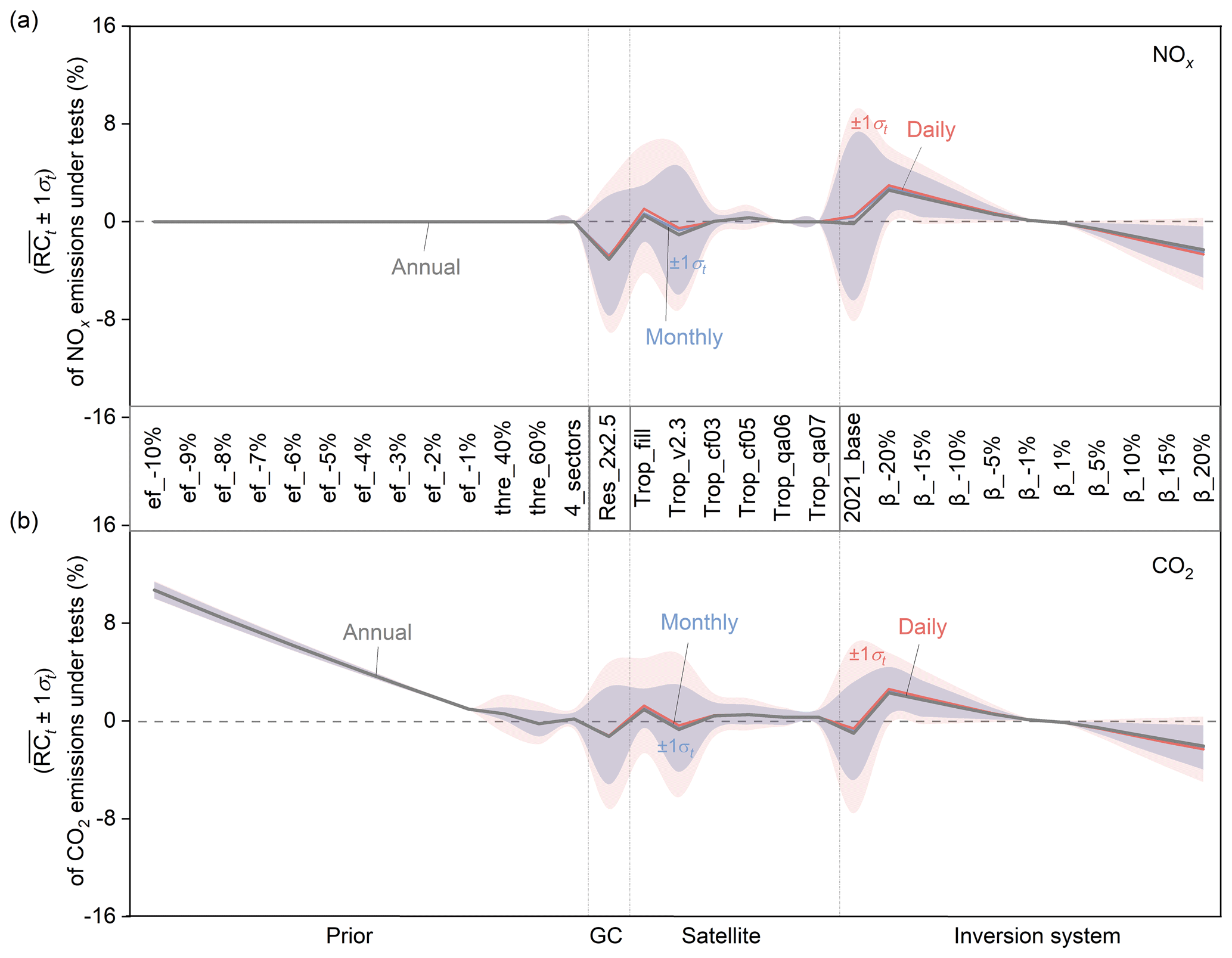
Figure 3 Comparison of the impacts of various tests on national total (a) NO_x and (b) CO₂ emissions at different timescales. Gray lines correspond to the RC_t in annual emissions. Blue lines depict the average RC_t in monthly emissions, with the shaded blue area indicating monthly-scale 1σ_t. Red lines illustrate the average RC_t in daily emissions, accompanied by the shaded red indicating daily-scale 1σ_t.

At the national total scale, prior tests (ef_[−10 %, −1 %], thre_40 % $/$ 60 %, and 4_sectors) influence CO₂ emissions consistently over time while leaving NO_x emissions unaffected (Fig. 3). This occurs because these tests only impact sectoral attribution and CO₂-to-NO_x emission ratios. Total NO_x emissions are determined in the top-down process before sectoral attribution, thus remaining unchanged (Fig. S1). However, sector-specific CO₂ emissions, derived from NO_x emissions, are influenced due to the varying CO₂-to-NO_x emission ratios among sectors (Fig. S10). A reduction in NO_x EFs increases rNO_x, thereby increasing the sectoral CO₂-to-NO_x emission ratios since CO₂ EFs are assumed to be unchanged (Eq. 5). This results in a linear elevation of CO₂ emissions in tandem with the decreased NO_x EFs (Fig. S7), with CO₂ emission variations reaching up to 10.7 ± 0.7 % under ef_−10 %. Similarly, modifications in threshold values and sector classification alter the identification of dominant sectors per grid, changing the sectoral attribution. Thre_40 %, thre_60 %, and 4_sectors bring about $\stackrel{\mathrm{‾}}{{\text{RC}}_t}\pm \mathrm{1}{\mathit{\sigma }}_t$ of 0.6 ± 1.5 %, −0.2 ± 1.7 %, and 0.2 ± 0.8 % in CO₂ emissions, respectively, demonstrating their low influence on emission estimates. Despite differences in the magnitude of prior tests' impacts ($\stackrel{\mathrm{‾}}{{\text{RC}}_t}$), they share a consistency at finer temporal scales, with daily 1σ_t below 4.0 %.

Changes in model resolution (Res_2 × 2.5) introduce the largest variation in estimates among all sensitivity tests, triggering $\stackrel{\mathrm{‾}}{{\text{RC}}_t}\pm \mathrm{1}{\mathit{\sigma }}_t$ of −1.2 ± 6.0 % in daily CO₂ emissions. Its notable inconsistency of impact on the finer temporal scale (1σ_t > 4.0 %) can be traced back to its induced spatiotemporally diverse changes in β (Fig. S11a and b). The overall low estimate of β under Res_2 × 2.5 results in negative RC_t, and the uneven spatial distribution of β explains the large 1σ_t.

As for the impact of satellite constraint, the systematic changes such as missing value supplementation (Trop_fill) or version changes (Trop_v2.3) have a larger impact with daily CO₂ emission variations of 1.3 ± 3.9 % and −0.4 ± 5.9 %, while alterations in satellite data quality screening conditions (Trop_cf/Trop_qa) exert a relatively minor impact on estimates with $\stackrel{\mathrm{‾}}{{\text{RC}}_t}$ ± 1σ_t less than 0.5 ± 1.8 %. The spatiotemporal changes in satellite NO₂ retrievals contribute to the inconsistent effects of Trop_fill and Trop_v2.3 on daily emissions. However, the small 1σ_t in screening condition tests suggests that the uncertainty in satellite retrievals has a minor impact on estimates unless there are systematic changes, possibly because we used the 10 d moving average of satellite observation data to constrain emissions.

Among inversion system parameter tests, the alteration of the reference year (2021_base) exhibits a notable temporally inconsistent impact, with $\stackrel{\mathrm{‾}}{{\text{RC}}_t}$ ± 1σ_t of −0.6 ± 6.9 % in daily CO₂ emissions. This inconsistency can be attributed to the spatiotemporally diverse changes in β, similar to the model resolution test (Fig. S11c and d). In contrast, changes in β (β_[−20 %, 20 %]) exert a more notable but consistent impact on estimates, linearly strengthening as the tested amplitude increases (Fig. S7), with β_−20 % triggering variations of 2.6 ± 3.0 % in CO₂ emissions. The spatiotemporally uniform changes in β act linearly on the inversion estimate of NO_x emissions (Eq. 1) and then on CO₂ emissions. Therefore, their impact remains consistent on a daily scale.

3.3 Emission sensitivity across source sectors

Regarding daily national sectoral NO_x and CO₂ emissions, their responses to different sensitivity tests, in terms of both emission magnitude and consistency $(\stackrel{\mathrm{‾}}{{\text{RC}}_s}\pm \mathrm{1}{\mathit{\sigma }}_s)$, are largely similar, except for NO_x EF tests (ef_[−10 %, −1 %]) (Fig. 4). Therefore, we primarily discuss the impacts of tests on sectoral emissions using CO₂ as a representative (refer to Sect. S4 for discussion on sectoral NO_x emission) and then delve into elucidating the divergent impact of NO_x EFs on sectoral NO_x and CO₂ emissions.

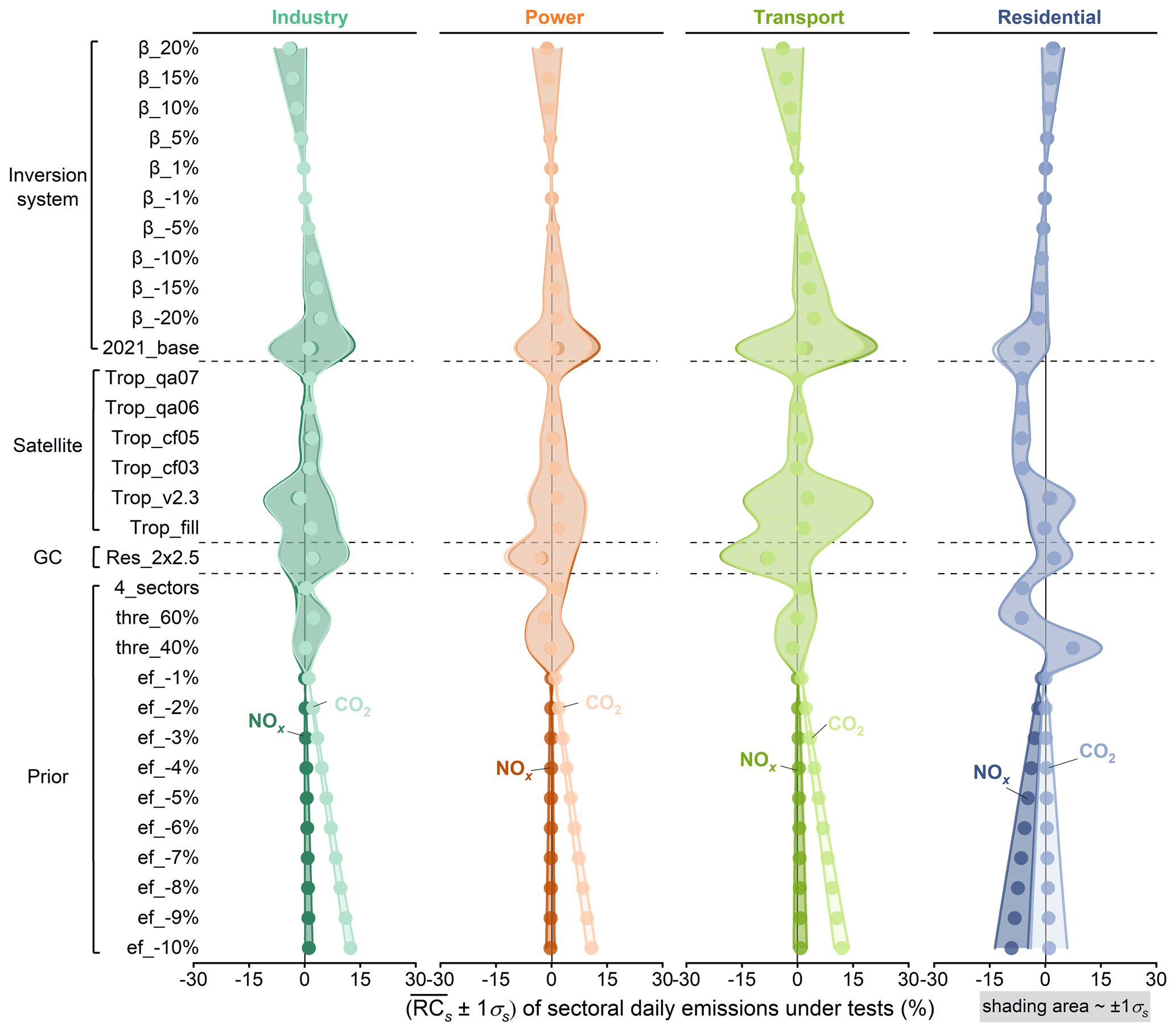
Figure 4 Response of sectoral national NO_x and CO₂ emissions to different sensitivity tests on a daily scale. From left to right, the panels correspond to the (a) industry, (b) power, (c) transport, and (d) residential source sectors, as the label notes. The dots inside each figure are the average RC_s of daily NO_x (deep color) and CO₂ (light color) emissions incurred by corresponding tests. The shaded area indicates the 1σ_s of RC_s of daily sectoral emissions in different tests.

Irrespective of NO_x emission factor changes (ef_[−10 %, −1 %]), industrial and power emissions exhibit greater robustness than transport and residential emissions, which are more susceptible to different configurations. Specifically, residential emissions demonstrate the highest susceptibility to reference year, showing $\stackrel{\mathrm{‾}}{{\text{RC}}_s}\pm \mathrm{1}{\mathit{\sigma }}_s$ of up to −6.7 ± 7.3 % in CO₂ emissions in 2021_base test, and exclusively display notable sensitivity to prior tests (4_sectors and thre_40 % $/$ 60 %) compared to other sectors (Fig. 4). In contrast, transport emissions are notably influenced by model resolution, with Res_2 × 2.5 incurring CO₂ emission variations of −7.8 ± 12.2 %. Among all sensitivity tests, the model resolution stands out as the most influential factor on sectoral emissions, because the resolution of grid cells affects the determination of the dominant source sector.

The overall largest sensitivity of residential emissions to sensitivity tests is potentially attributed to its low proportion to total emissions (Fig. S12). Take thre_40 % $/$ 60 % as an example: lowering the threshold from 50 % to 40 % results in identifying more grids as residential-source-dominant. This, in turn, leads to an increase in residential emission proportions when allocating the total TROPOMI-constrained NO_x emissions into sectors and subsequently CO₂ emissions. Conversely, fewer grids are assigned as residential-dominant when the threshold rises from 50 % to 60 %, resulting in lower residential emissions (Fig. S13). The next sensitive sector is transport, particularly vulnerable to model resolution, which may be associated with its characteristics in spatial distribution. Transport-dominant grids, particularly those with truck emissions, are typically located close to industry-dominant grids whose NO_x emissions outweigh those of the transport (Zheng et al., 2020). The use of coarser horizontal resolution could result in a diminished attribution of emissions to transport (Fig. S14).

The reduction in NO_x EFs (ef_[−10 %, −1 %]) is the only test impacting sectoral NO_x and CO₂ emissions differently. For NO_x emissions, the residential sector shows the strongest sensitivity with $\stackrel{\mathrm{‾}}{{\text{RC}}_s}\pm \mathrm{1}{\mathit{\sigma }}_s$ of up to −9.1 ± 4.5 % under ef_−10 %. However, its influence on CO₂ emissions is most pronounced in all sectors except residential, with variations of 12.4 ± 1.1 % in CO₂ emissions from industry, 11.9 ± 1.9 % from transport, and 10.8 ± 1.2 % from power but only 1.0 ± 4.9 % from residential sectors under ef_−10 %. The reduction in NO_x EFs shifts the dominant sector attribution, substantially lowering NO_x emissions from the residential sector due to its vulnerability to these changes, similar to the impact seen with the thre_60 %. The other sectoral (industry, transport, and power) CO₂ emissions present stronger sensitivity to NO_x EF tests, linearly correlated with the extent of EF changes. The decline in sectoral NO_x EFs linearly reduces rNO_x (Eq. 5), raising the corresponding CO₂ emissions by increasing sectoral CO₂-to-NO_x emission ratios.

3.4 Emission sensitivity at subnational scales

Refining spatial coverage from national to subnational level (i.e., province) reveals that factors causing inconsistent impacts over finer timescales also tend to induce inconsistent impacts on more granular spatial regions (Fig. 5). On annual total scales, the RC_p of NO_x and CO₂ emissions at the provincial scale closely resemble each other under most sensitivity tests, except for prior tests that only influence CO₂ emissions (Fig. S15). When comparing across provinces, the sensitivity of emissions to tests correlates with the size of the provincial area, with smaller regions exhibiting greater susceptibility. Shanghai, the smallest provincial-level administrative unit in China in terms of area, experiences the largest RC_p throughout China in nearly all tests. Conversely, Inner Mongolia, one of China's top three largest provinces, undergoes the minimum RC_p in all tests. Under Res_2 × 2.5, the RC_p of annual total NO_x and CO₂ emissions in Shanghai are 19.6 % and 22.6 %, respectively, while in Inner Mongolia, they are −3.2 % and −3.3 %. Employing a resolution of 2° × 2.5° in Shanghai is impractical in real-world applications, as it would result in fewer than two grids covering the area. Henan also encounters substantial RC_p under Res_2 × 2.5, reaching as high as −15.8 % and −12.4 % in annual total NO_x and CO₂ emissions. This could be attributed to its proximity to Shandong, a province with approximately twice the emissions of Henan, making Henan particularly sensitive to the changes in model resolution due to the overlapping grid cells. It is noteworthy that Guizhou exhibits the highest sensitivity to satellite constraints, with RC_p reaching up to 11.9 % and 11.8 % in annual total NO_x and CO₂ emissions under Trop_v2.3. This sensitivity is attributed to the high cloudiness of the Yunnan–Guizhou Plateau, causing satellite observations to be highly uncertain over Guizhou (Wang et al., 2023; Li et al., 2021; Cai et al., 2022).

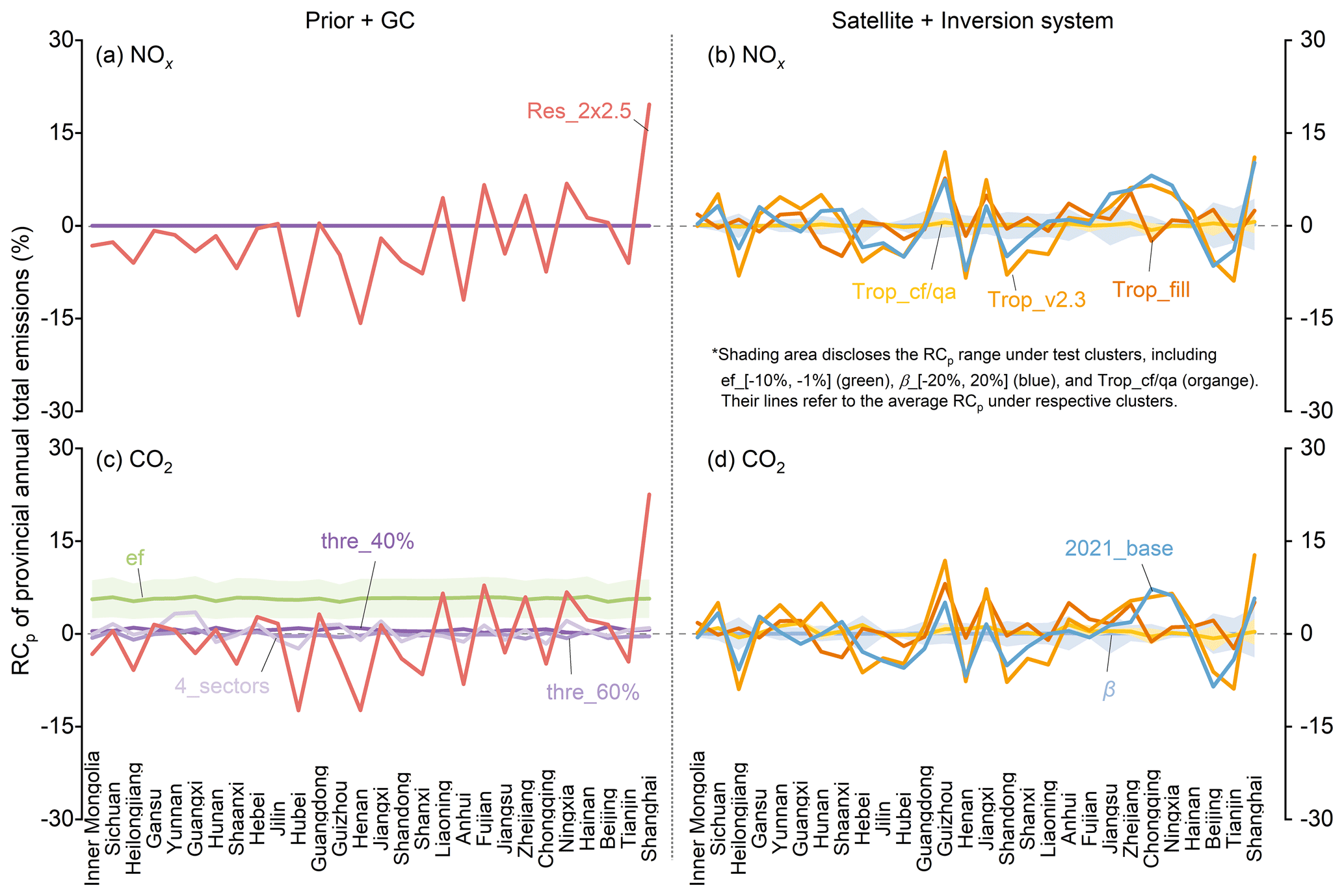
Figure 5 Response of provincial annual total NO_x and CO₂ emissions to different tests. Panels (a) and (b) show RC_p of NO_x emissions incurred by tests. Panels (c) and (d) are plotted for CO₂ emission as panels (a) and (b). Lines refer to the RC_p caused by the corresponding test or the averaged RC_p caused by corresponding test clusters (ef_[−10 %, −1 %] and β_[−20, 20 %]), and the shaded area refers to the RC_p range in test clusters. Only provinces with enough TROPOMI observations are shown here (i.e., grids with NO₂ TVCDs larger than 1×10¹⁵ molec. cm⁻² cover more than 90 % of anthropogenic NO_x emissions within provinces). The provinces are arranged by area.

To further investigate the daily total emission response $(\stackrel{\mathrm{‾}}{{\text{RC}}_{\mathrm{r}}}\pm \mathrm{1}{\mathit{\sigma }}_{\mathrm{r}})$ to tests at the regional scale, we select and analyze Jing–Jin–Ji (JJJ, including Beijing, Tianjin, and Hebei) clusters; Inner Mongolia; Yangtze River Delta (YRD) clusters (including Shanghai, Zhejiang, and Jiangsu); and Guangdong (the location of the Pearl River Delta). These regions respectively represent an industrialized region with high population density, an industrialized region with sparse population density, and two major economic development zones with high population density in China (Fig. 6). Geographically, these regions span northern China (JJJ and Inner Mongolia), eastern China (YRD), and southern China (Guangdong), thereby covering different meteorological and geographic factors. Overall, the $\stackrel{\mathrm{‾}}{{\text{RC}}_{\mathrm{r}}}\pm \mathrm{1}{\mathit{\sigma }}_{\mathrm{r}}$ of daily regional emissions are similar for NO_x and CO₂ except for ef_[−10 %, −1 %], resembling their daily national emission responses (Fig. 3). The $\stackrel{\mathrm{‾}}{{\text{RC}}_{\mathrm{r}}}\pm \mathrm{1}{\mathit{\sigma }}_{\mathrm{r}}$ of daily regional emissions is especially notable in YRD and Guangdong (southern part of China). This could be attributed to the relatively low NO₂ concentration in southern China (Fig. S4), making them particularly sensitive to spatial variations in parameters, such as the β in 2021_base (Fig. S11) and NO₂ TVCDs in the Trop_v2.3 test. Besides, the cloud fraction is higher in southern China, introducing larger uncertainties in remote sensing (Liu et al., 2019; Latsch et al., 2022). The emission responses to prior and β_[−20 %, 20 %] tests are close for these four regions, particularly in the prior tests, suggesting that these impacts on emissions are less dependent on geographic factors.

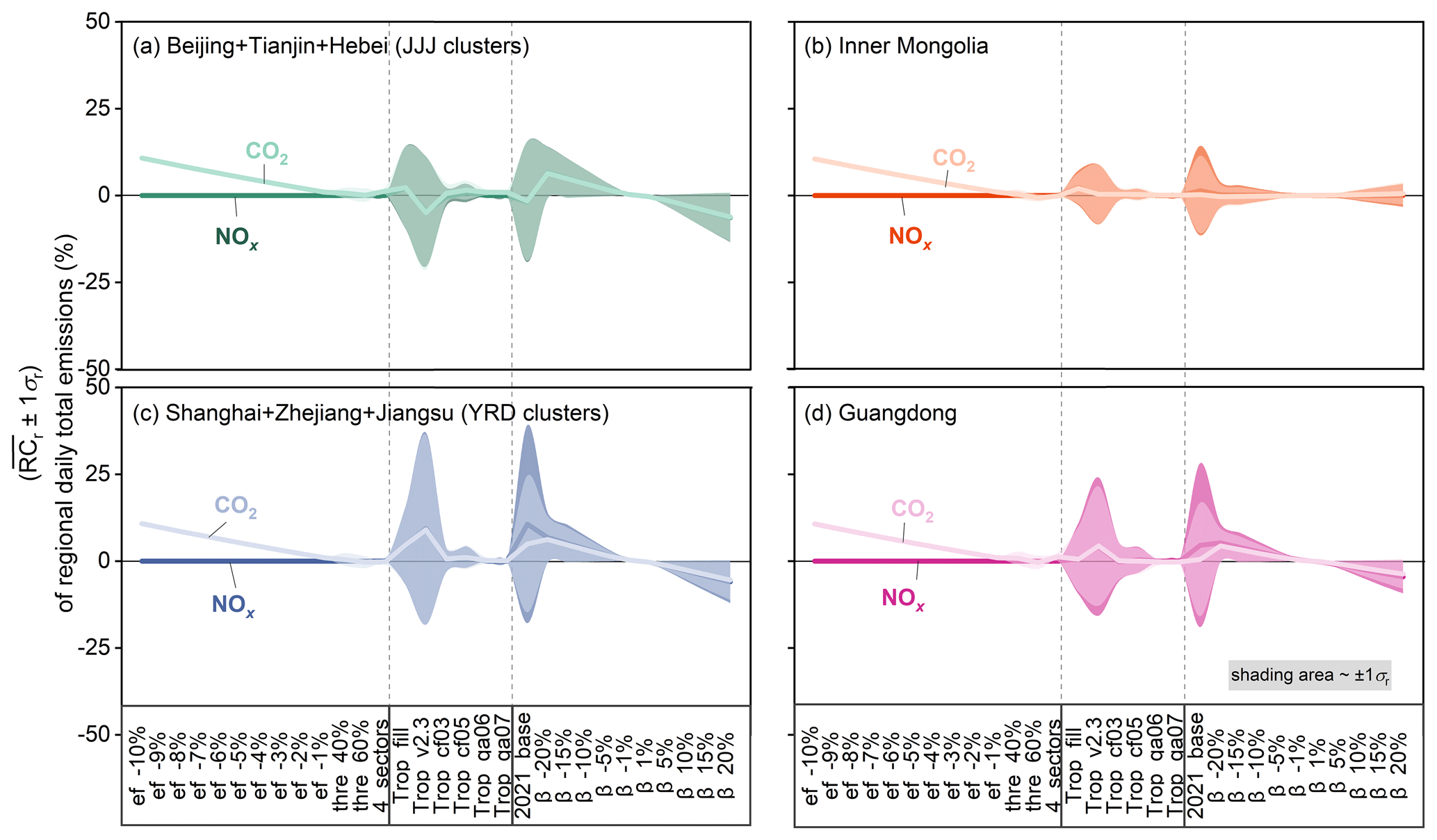
Figure 6 Response of regional total NO_x and CO₂ emissions to tests on a daily scale. Panels (a), (b), (c), and (d) show the $\stackrel{\mathrm{‾}}{{\text{RC}}_{\mathrm{r}}}\pm \mathrm{1}{\mathit{\sigma }}_{\mathrm{r}}$ of daily NO_x (deep color) and CO₂ (light color) emissions in different tests in Jing–Jin–Ji clusters (Beijing, Tianjin, and Hebei); Inner Mongolia; Yangtze River Delta clusters (Shanghai, Zhejiang, and Jiangsu); and Guangdong. The shaded area inside each figure refers to the corresponding 1σ_r. It is worth noting that the Res_2 × 2.5 test is not shown here since the resolution of 2° × 2.5° proves too coarse for certain regions, rendering it unrealistic for real-world applications. The result containing Res_2 × 2.5 is present in the Supplement as Fig. S16 for reference.

4 Discussion

This study delineates an approximate spectrum of uncertainties inherent in deriving conclusions of varying precision with our air-pollution-satellite-based CO₂ emission inversion system. When interpreting conclusions based on the emission data derived from such an inversion system, it is practical and imperative to aggregate emissions across different dimensions to fulfill specific usage requirements. Direct utilization of data with all fine-grained resolutions at temporal, sectoral, and spatial dimensions poses challenges. If adhering to a variation tolerance of 5 %, the reliability of annual national NO_x and CO₂ emissions is established in most cases. Notably, careful attention is needed when selecting model resolution and attributing sectoral emissions. Expanding the tolerance to 10 %, which is still below the conventional bottom-up method's uncertainty range of 13 %–37 % (Zhao et al., 2011; Huo et al., 2022), renders annual regional or daily national emissions robust from an average perspective. Nevertheless, meticulous scrutiny is advised when drawing conclusions based on daily sectoral or daily regional emissions, especially in specific regions (e.g., Shanghai, Guizhou). The large uncertainty of daily sectoral emission is typically observed in other emission datasets, such as the Carbon Monitor dataset (up to 40 % uncertainty) (Liu et al., 2020; Huo et al., 2022). Further liberalizing the tolerance to 25 %, which is quite uncertain for scientific and policy-making purposes, a majority of conclusions derived from our estimates stand as reliable. The extensive tolerance range primarily stems from regional emissions, posing a challenging issue for many emission inversion techniques. For example, the uncertainty in NO_x emissions derived from the 2D MISATEAM (chemical transport Model-Independent SATellite-derived Emission estimation Algorithm for Mixed-sources) method is approximately 20 % for large and mid-size US cities (Liu et al., 2024), and the uncertainty for daily NO_x and CO₂ emissions based on the superposition model ranges from 37 % to 48 % on a city scale (Zhang et al., 2023). Notably, remarkable advancements have been achieved in estimating subnational CO₂ emissions through CO₂-observing satellites, such as sectoral CO₂ assessments with OCO-3 (Roten et al., 2023) and urban emission optimizations utilizing the Orbiting Carbon Observatory-2 (OCO-2) (Yang et al., 2020; Ye et al., 2020). Yet reducing uncertainties at subnational scale remains an ongoing challenge.

This study paves the way for the continuous improvement of the current air-pollution-satellite-based CO₂ emission inversion system. Firstly, prioritizing a nimble and appropriate horizontal resolution is crucial for establishing accurate localized relationships between NO₂ TVCDs and NO_x emissions, contributing to improved NO_x and CO₂ emission estimations from temporal, sectoral, and spatial perspectives. Secondly, the more accurate satellite observation is conducive to reducing the uncertainty in final results, presenting increasing promise with advancements in remote sensing technology. Besides, the progress in multi-species synchronous observations through satellite and aircraft platforms offers alternative verification for multi-species emission inversion, such as the Copernicus Anthropogenic Carbon Dioxide Monitoring constellation (CO2M) (Sierk et al., 2021). Thirdly, the reliability of sectoral NO_x EF changes, which determine CO₂-to-NO_x emission ratios, is essential for the accurate conversion from NO_x to CO₂ emissions. This underscores the need to acquire more accurate NO_x EFs. While obtaining on-site measurements of CO₂-to-NO_x emission ratios is challenging, efforts are underway to enhance its configuration. An iterative modification of NO_x EFs within the current system could be incorporated, minimizing the gap between bottom-up updated and TROPOMI-constrained sectoral NO_x emissions to below 2 %. This approach yields more accurate CO₂-to-NO_x emission ratios and CO₂ emissions (Fig. S17). The optimized CO₂ emission change from 2021 to 2022 is +0.6 %, reflecting a more precise representation of the growth in fossil fuel consumption (+1.9 %). Fourthly, utilizing a more refined approach to determine dominant sectors at a grid level can reduce the uncertainty of sectoral emissions with lower contributions, particularly in the residential sector. These enhancements will improve the system's accuracy in estimating emissions across all dimensions, positioning it as a valuable tool for simultaneous inversion-based monitoring of greenhouse gas and air pollutant emissions, ultimately supporting a strategic roadmap for the vision of clean air and climate warming mitigation.