High resolution air quality simulation in the Himalayan valleys, a case study in Bhutan

Our study focuses on Bhutan, a highly mountainous country where government authorities are strengthening air pollution monitoring efforts. To support further analysis and the monitoring strategy, we present the first high-resolution air quality simulations with the chemistry transport model WRF-CHIMERE over the western region of Bhutan at a spatial resolution of roughly 1 km. Increasing the horizontal resolution of the model improves its performance and reduces potential errors caused by excessive spatial averaging of meteorological and emission data with high spatial variability. However, the air pollutant emissions must be improved at a fine scale with better proxy, particularly for industries where improvements are still required. For the first time, we propose high resolution maps of air pollution (concentrations and deposition fields). Our simulations confirm that Bhutan valleys also suffer from air pollution mainly due to PM_2.5 (concentrations exceeding 20 µg m⁻³) dominated by carbonaceous species, largely above the World Health Organization guidelines. Wildfires and anthropogenic activities release large amount of carbonaceous species and can also impact the glaciers by atmospheric fallout. Wildfires can locally contribute to 20 % of the total PM_2.5 concentrations over a 15 d period, and theoretically, black carbon can be transported up to the highest peaks. Ecosystems are at risks with deposition fluxes of sulfur and nitrogen species comparable with other locations at risk in the world.

1 Introduction

The Hindu Kush Himalaya (HKH) spans over a region particularly affected by air pollution including India, Pakistan, Bangladesh and Nepal which are currently the most impacted by air pollution (HEI, 2025; Mehra et al., 2019). Particularly outside the monsoon season, the combination of favorable meteorological conditions and large emission sources in the Indo-Gangetic Plain is the main reason of impressive outbreak of pollution events. In the region, air pollution not only affects health (HEI, 2025). Air pollution also has an effect on ecosystems (loss of biodiversity) through the deposition of inorganic species like ammonia (Beachley et al., 2024) as explained by Bhagowati and Ahamad (2019), and on the melting of glaciers (Gul et al., 2021; Kang et al., 2020) due to deposition of Black Carbon on snowy surfaces. Particles have also an effect on meteorological conditions and implications on the development of the monsoon in the region (Santra et al., 2025; Hassan et al., 2023). Environmental risks in HKH related to climate change directly or indirectly affect around 2 billion people in Asia.

Bhutan, the smallest country in the region, is bordered to the north by China and to the west, south, and east by India. The country is crisscrossed by numerous rivers that flow southward, creating a number of deep valleys where the most significant cities are located. These include the capital, Thimphu, which is at 2400 m a.s.l., Paro, which has the country's only international airport, and Haa, which is close by and reachable from Paro via a pass at 3900 m a.s.l. The elevation varies from more than 7000 m in the north to 200 m in the south near the Indian border. Bhutan is considered as a pristine environment and looks less affected by air pollution compared to its neighbors. Bhutan is covered by 70 % of forest, and a particularity of this country is the exposure of its population to indoor air pollution mainly due to cooking activities and heating systems using wood (Wangchuk et al., 2015; Pratali et al., 2019; Khumsaeng and Kanabkaew, 2021).

Traditional wood-burning stoves, called Bukhari are extensively used for heating and cooking (Wangchuk et al., 2017). These residential combustion sources in deep valley has an effect on ambient air concentrations, they represent more than 80 % of primary PM_2.5 (Particulate Matter with diameter below 2.5 µm) emissions according to the EDGAR (Emission Database for Global Atmospheric Research) emission database (Crippa et al., 2024; Guizzardi et al., 2025). Along the year, PM_2.5 concentrations range on a monthly basis from less than 20 µg m⁻³ during the monsoon to more than 40 µg m⁻³ in wintertime (Sharma et al., 2021), largely above the WHO (World Health Organization) guidelines of 5 µg m⁻³ for PM_2.5 (WHO, 2023, 2021). The Royal Government of Bhutan is a leading country to fight against air pollution, the Thimphu Outcome summarizes the key discussions and recommendations from the Second Regional Science Policy Dialogue on Air Quality Management in the Indo-Gangetic Plain and Himalayan Foothills (IGP-HF) held on 26–27 June 2024, co-organized with ICIMOD and the World Bank (ICIMOD and World Bank, 2024).

Western Bhutan’s air quality is often deteriorated due to continuous forest fires during pre-monsoon, and then climate change may place rural livelihoods at risk (Vilà-Vilardell et al., 2020) with more and more favorable conditions leading to outbreak of fires. In the region the effect of forest fires on air quality has been studied by Kumari et al. (2024) indicating the urgent need for targeted interventions to mitigate the impact of forest fires on air quality in the North-East of India close to Bhutan. According Karthik et al. (2022), in India, vegetation burning contributes more than 80 % of carbon stock. In Bhutan a recent study (Sharma et al., 2022) estimated the potential source regions contributing to the PM_2.5 concentrations in Thimphu during the years 2018–2020 using a Lagrangian model. They showed that 80 % of PM_2.5 were due to external sources mainly coming from India. However, for the country, there is a need to set-up a more robust and comprehensive modeling platform to analyse the role of each sources to tailor the more appropriate mitigation strategies and enhance a regional dialogue to collectively curb air pollution in the region.

The use of models in such an area is challenging and combines several difficulties related both to the reconstruction of air pollutant emission inventories at high resolution and the simulation of meteorology in such a mountainous zone (Singh et al., 2024). The issue of the spatial resolution of models to simulate the Black Carbon (BC) deposition fluxes was highlighted by Kang et al. (2020) who considered crucial to increase their spatial resolution. Indeed, so far, models are mainly applied at coarse resolution around 10 km with emission inventories at similar resolutions. A recent study over Europe shows the added value of using high-resolution simulations to assess the impact on health and potential social inequalities, as emission reduction strategies have highly spatially heterogeneous consequences (Pisoni et al., 2025). This type of studies needs to be extended over the whole South Asia, and furthermore we must prepare high resolution simulations in the region to train super-resolution models based on deep-learning techniques to address the air quality at the urban scale over wide domains with complex topography as initiated by Bessagnet et al. (2021).

While Ciarelli et al. (2025) recently focused at 1 km resolution over Nepal to estimate the role of nucleation in the formation of ultrafine biogenic particles, our study is the first to evaluate the air quality and deposition fluxes of key atmospheric species with a chemistry transport model with a 1 km resolution in several Himalayan valleys of the West of Bhutan, Haa, Paro, Thimphu and Punakha. The objective of our study is fourfold: (i) evaluate the performance of the CHIMERE model against available ground observations and set-up a stable framework, (ii) propose a first cartography of the potential impact of air pollution, (iii) evaluate the impact of forest fires and (iv) along the analysis, evaluate the role of the spatial resolution of the model in such a complex topography area.

2 Model set-up

The chemistry transport model CHIMERE (Menut et al., 2024a) coupled with the WRF (Weather Research Forecast) meteorological model (Skamarock et al., 2008), is used to simulate air pollutant concentrations for the period from 10 February to 31 March 2025. Five days prior to this period are used as a spin-up to initialize the concentration fields in the model. The period corresponds to a measurement campaign in Haa to evaluate indoor and outdoor exposure. This post-winter period is still cold in Bhutan with some morning frosts, and temperatures which can exceed 15 °C in the afternoon. As other locations in the Himalaya, the diurnal cycle of the winds is governed by strong daytime up-valley winds and weak nighttime winds (Potter et al., 2018; Mikkola et al., 2023). Katabatic winds in these areas are expected to have consequences on the transport of air pollutants from the highest layers of the atmosphere (Yang et al., 2015). Wildfires are commonly observed from March in Bhutan that is the beginning of the pre-monsoon period. Some light precipitations (rain and snow) in the valleys are observed during the studied period in Western Bhutan.

The CHIMERE model is a regional chemistry-transport model that can be used in both online and offline configurations in its latest version for research, scenario analysis and operational forecast purposes (Lapere et al., 2021; Bessagnet et al., 2020; Menut et al., 2020). Three domains are designed targeting the western part of Bhutan at 0.01° resolution (Figs. 1 and 2). The model needs a set of gridded data as mandatory input: emission data for both biogenic and anthropogenic sources, land use parameters, boundary and initial conditions, and other optional inputs such as dust and fire emissions. Given these inputs, the model calculates the concentrations and wet/dry deposition fluxes for a list of gaseous and aerosol species (depending on the chosen chemical mechanism).

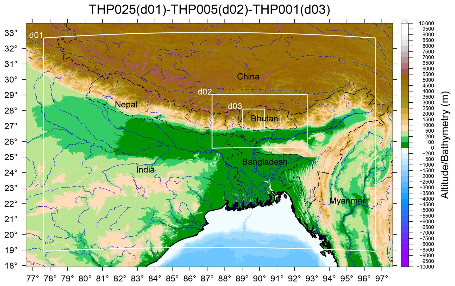
Figure 1 Simulation domains (white frames) in our study.

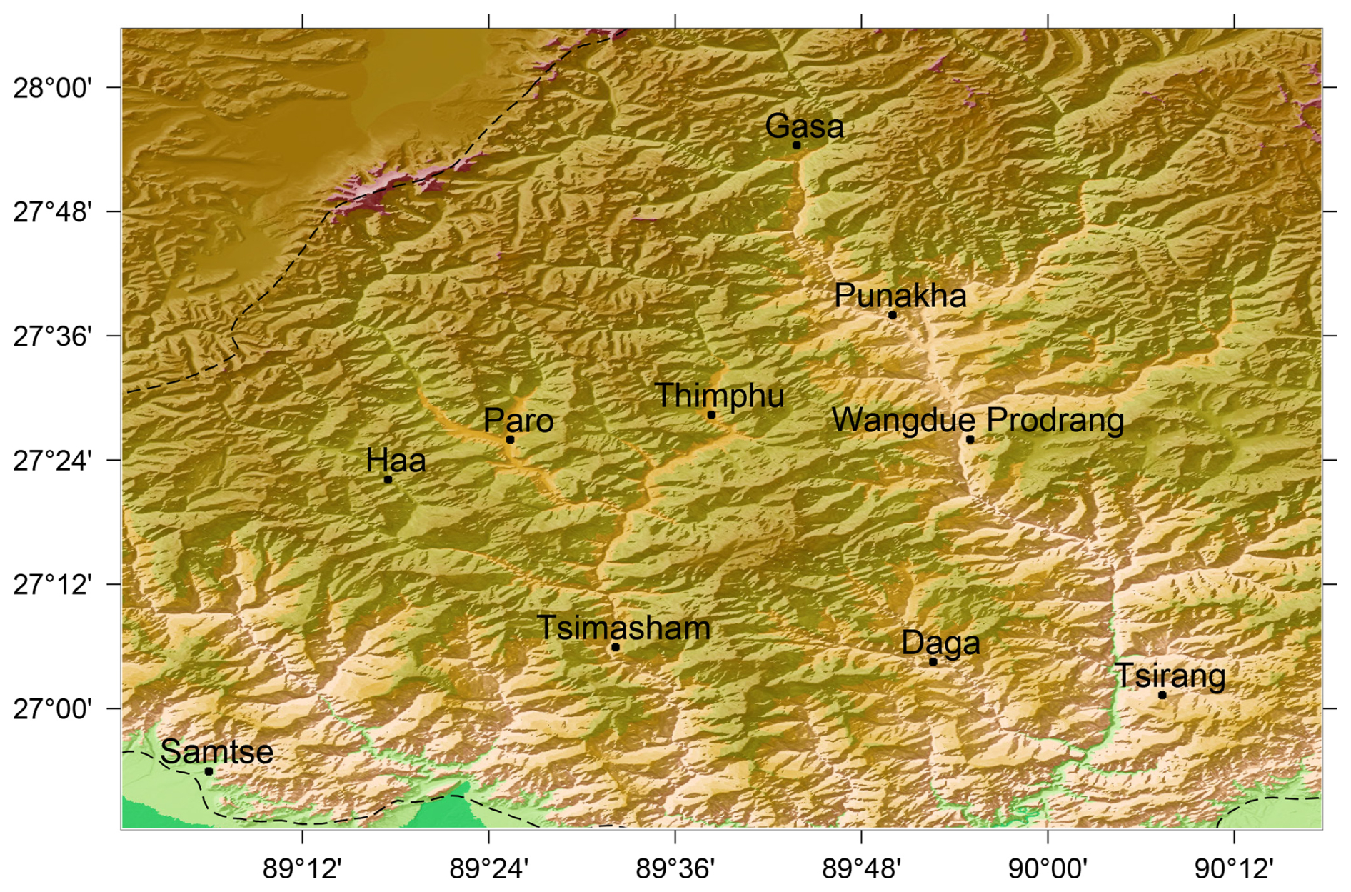
Figure 2 High resolution domain THP001/d03 over Western Bhutan. The highest mountains (Jomolhari – 7326 m – and Jichu Drake – around 6800 m) are located over the North-West part of the domain along the border with China. The main valley are cleary identified, Haa being a high altitude valley.

In this study, the model is coupled with WRF using the NCEP raw data (National Centers for Environmental Prediction) at 1° × 1° (Kalnay et al., 1996) for the global meteorological conditions and initialization. The WRF-CHIMERE suite is run on a triple nested configuration, with a coarse domain covering the HKH at a 0.25° × 0.25° resolution (THP025/d03), the intermediate domain over the whole Bhutan with a 0.05° × 0.05° resolution (THP005/d02), while the finest domain focused on the West Bhutan region with at a 0.01° × 0.01° resolution (THP001/d03). As described in Sect. 3, we have developed a fine emission inventory at 0.01° × 0.01° resolution so that the three simulations longitude/latitude regular domains are a multiple of the emission grid: ×1 for THP001, ×5 for THP005 and ×25 for THP025 (Fig. S1 in the Supplement). The CHIMERE vertical resolution contains 20 layers starting from the surface going up to 200 hPa. For the WRF configuration we have increased the resolution with 46 eta-levels until 30 hPa to account for the complex topography. The various WRF parameters are similar of those used in Bessagnet et al. (2020) where a simulation over a complex topography was performed with an evaluation of the vertical patterns. Fire emissions fluxes are calculated from daily CAMS Global Fire Assimilation System (Copernicus Atmosphere Monitoring Service, 2022). The data used are the analysis and have an horizontal resolution of 0.1 × 0.1°, (Kaiser et al., 2012). These data are reformatted to be consistent with the required CHIMERE input data. This procedure includes: (1) spatially, the data are projected on the CHIMERE horizontal model grid, (2) temporally, these daily data are interpolated to provide hourly fire emission fluxes, (3) chemically, the chemical species are disaggregated and reaggregated to be consistent with the model chemical mechanism. The injection height is calculated using the scheme of Sofiev et al. (2012) requiring the Fire Radiative Power (in Mega Watts). Vertically, the shape of the emission profile is calculated using a profile defined and described in Menut et al. (2018). The accumulation of burnt areas is calculated and allows to calculate the impact of fires on the surface then mineral dust emissions, biogenic emissions and dry deposition as explained in Menut et al. (2022) and Menut et al. (2023). Spectral nudging is applied for the coarse domain THP025. The wind components, the potential temperature perturbation and the water vapor mixing ratio are nudged with a relaxation coefficient g=0.0003 s⁻¹. A wave number of 5 and 4 is used, respectively on x and y directions. For this exercise, all simulations are made off-line without feedback (radiative effects) of aerosols on the meteorology.

The resuspension scheme is activated within the domain (Vautard et al., 2005), it does not include road traffic resuspension. The resuspension process is important for particulate matter and may induce a large increase of the emission flux in the case of dry soils, for locations where traffic and industries produce available particles. This resuspension process is considered as different and complementary to the aeolian erosion process which is not activated for our domains (no relevant arid zones in the region of interest). Biogenic VOC emissions are computed online with the MEGAN 2.10 algorithm (Guenther et al., 2012). Boundary conditions were taken as monthly climatologies from LMDz-INCA (Hauglustaine et al., 2014) as standard data provided in the CHIMERE package. For mineral dust, we use the monthly climatologies at the boundaries from the GOCART model which is more adapted for our analysis on dust deposition since we want to capture an average behaviour for a month (Sect. 6.2). Dust episodes are very sporadic with a strong temporal variability, as explained in Vautard et al. (2005), the monthly median value of dust as boundary conditions is used instead of the average concentration.

All major aerosol groups are activated in the model including elemental carbon, organic matter, sulfate, nitrate, ammonium, SOA (Secondary Organic Aerosols), mineral dust (from the boundaries), sea salts, and PPM (here non-carbonaceous Primary Particle Matter and resuspended particles); taking into account coagulation, nucleation and condensation processes over 10 size bins ranging between 10 nm–40 µm. The chemical formation of SOA from primary organic aerosol is not activated here. Wet scavenging and dry deposition is considered following the Wesely's parameterization (Wesely, 1989). For more details, the WRF and CHIMERE configuration files are provided in Table S1 and S2.

3 Anthropogenic emissions

There is no available high resolution air pollutant emissions inventory in the region. We use the procedure developed by Bessagnet et al. (2023) to create an emission inventory at fine scale (0.01° resolution) from a coarse resolution emission dataset. This methodology builds a high resolution inventory based on proxy for each activity sector of a coarse emission database. Our coarse emission inventory at 0.1° × 0.1° is the EDGAR database (Crippa et al., 2024) for the year 2022 and the main pollutants such as CO, PM₁₀, PM_2.5, Organic Matter assuming OM $=\mathrm{1.6}\times$ OC according Philip et al. (2014), and accessible at https://edgar.jrc.ec.europa.eu/dataset_ap81 (last access: 11 December 2025), BC, SO₂, NO_x, NH₃, NMVOC (Non-methane Volatile Organic Compounds). Primary OM (Organic matter) and BC is considered in the fine fraction PM_2.5. We have then developed a 0.01°×0.01° over the whole South Asia for the same pollutants. For the residential sector (RCO) and the traffic emissions (TRO), the downscaling has been applied from the country level to the fine grid. For the industrial and all other remaining sectors, we prefer to use the downscaling from the EDGAR grid to benefit from a first spatialisation embedding more information at sub-national level. Moreover, EDGAR data are provided over 36 possible classes of activity sectors for annual emissions and 8 macro sectors for monthly emissions (Table S3). Therefore, we have calculated monthly profiles over the 8 macro sectors and applied them to the 36 possible sub-categories to maximize the use of information.

Bhutan’s emission profile reflects its economy, which is primarily based on agriculture, livestock, forestry, mining, hydropower exports to India, and tourism. Emission data for Bhutan extracted from the EDGAR database (Table 1) indicate that residential emissions (RCO) contribute the largest share of most compounds. NO_x emissions mainly originate from the residential, industrial, and traffic sectors. A distinctive feature of Bhutan is the dominance of the residential sector, which is the largest emitter of both NO_x and NH₃, whereas in neighboring countries such as India, traffic and agriculture are the main sources of these pollutants, respectively. Although agriculture is often cited as the primary source of ammonia, wildfire emissions are probably underestimated, as noted by Felix et al. (2023).

Table 1 Emission of air pollutants for Bhutan according EDGAR (kton in 2022) for main activity sectors reconstructed from the gridded data.

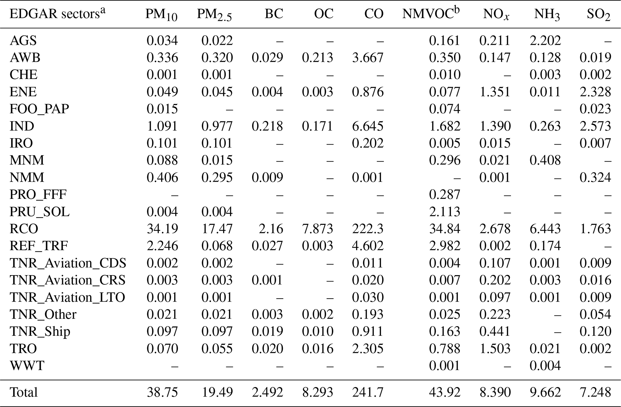
^a AGS: Agricultural soils, AWB: Agricultural waste burning, CHE: Production of chemicals, ENE:Energy, FOO:Food Production, IND:Combustion in manufacturing industry, IRO: Iron and Steel production, MNM:Manure Management, NMM: Production of non metallic minerals, PRO_FFF: Fuel Exploitation, PRU_SOL: Solvents, RCO: Small scale combustion, REF:Refineries, TNR_Aviation _CDS: Aviation climbing & descent, TNR_Aviation_CRS:Aviation cruise, TNR_Aviation_LTO: Aviation landing & takeoff, TNR_Aviation_SPS: Aviation supersonic, TNR_Other: Railways, pipelines, off-road transport, TNR_Ship: Shipping, TRO:Road Transport, WWT: Waste Water Treatment. ^b Non Methane Volatile Organic Compounds.

The global population database GHSL (Global Human Settlement Layer) developed by the European Commission – Joint Research Centre (Pesaresi et al., 2024) is used. These data at 100 m resolution were used to downscale the emissions from the residential sector (mainly heating, air conditioning and cooking operation).

Specific emissions from butter lamps and incense burning (Yangzom et al., 2024) in the context of religious rituals in Bhutan are not taken into account here. Another source related to road dust resuspension is particularly important in the winter and pre-monsoon period. For the residential sector, while for gas emissions we have directly used the population density to spatially reallocate the emissions, we use a different approach for particulate emissions. Indeed, these latter emissions are mainly emitted by wood burning mostly occurring in rural places. The methodology calibrated over Europe (Terrenoire et al., 2015) with bottom-up emissions gave a population-based proxy px^p for particulate species as a function of population density pop where the coefficient c is set to 1.5 here after several trials (Eq. 1).

$$\begin{array}{}\text{(1)}& {\mathrm{px}}^{\mathrm{p}}=\mathrm{pop}\times {\left[{\log }_{\mathrm{10}}\left(\mathrm{pop}\right)\right]}^{-c}\end{array}$$

In short, the proxy is used to calculated the high resolution emission e in a high resolution grid cell i as in Eq. (2) for a downscaling of emission E of the coarse level structure C which is either the country or the corresponding coarse grid cell.

$$\begin{array}{}\text{(2)}& e_{i\in C}=E_C\times {\displaystyle \frac{{\mathrm{px}}_i}{\sum _{j\in C}{\mathrm{px}}_j}}\end{array}$$

This formula indicates that PM emission per capita is more important in rural places due to more frequent use of wood for heating and cooking (Denier van der Gon et al., 2015). This behavior is very usual worldwide, households use the resource that is the less expensive and very accessible in their close environment. This methodology allows differentiation between wood and non-wood sources of gaseous and particulate emissions. As reported in the European Environment Agency guidebook on air pollutant emissions (EEA, 2023), the $\mathrm{PM}/{\mathrm{NO}}_{\mathrm{x}}$ emission factor ratio is the largest for wood used in all stoves compared to LPG (Liquefied Petroleum Gas) or other fossil fuels burnt under more controlled combustion processes.

For most other proxy, the OSM (OpenStreetMap) project (OpenStreetMap contributors, 2024) is used and rasterized at 3 arcsec (about 90 m). Harbors, airports, industries, crops can then be spatially reallocated at the adequate resolution. We calculate a 3^′′ arcsec proxy which represents the percentage of surface occupied by a land cover. These proxy are then aggregated at 0.01° resolution in the downscaling procedure. For roads, to estimate the surface, a specific width in meters is assigned for each type of roads as: unclassified: 9 m, motor: 15 m, primary: 15 m, secondary: 12 m, tertiary: 7 m, residential: 5 m, footway: 3 m, service: 5 m. A pre-treatment is operated at $\mathrm{1}/\mathrm{3}$ arcsec (about 10 m) before reaggregation at 3 arcsec. One peculiarity in the region is the Brick Kiln industry, which is a major issues for the environment and human health. The brick kiln sector across South Asia, including the Himalayan region, operates largely in the informal economy, making it hard to regulate or relocate. Kilns are often scattered, unregistered, and invisible to policymakers, which complicates efforts to enforce environmental or labor standards. The stack are so complicated to localize that it is very challenging for the emission community to correctly account for this source (Tahir et al., 2021; Das et al., 2025). This specific sector is not isolated in EDGAR, then we reallocate spatially the emissions of this sector with a single industrial proxy from OSM.

As shown in Fig. 3, we can clearly see the added value of the downscaling procedure for two major activity sector. In the EDGAR raw database at coarse resolution, the main road in Bhutan cannot be identified while at fine resolution, the reallocation of the emissions provides a more realistic picture at 0.01° resolution. For instance, at coarse resolution the roads in the Haa Valley did not appear.

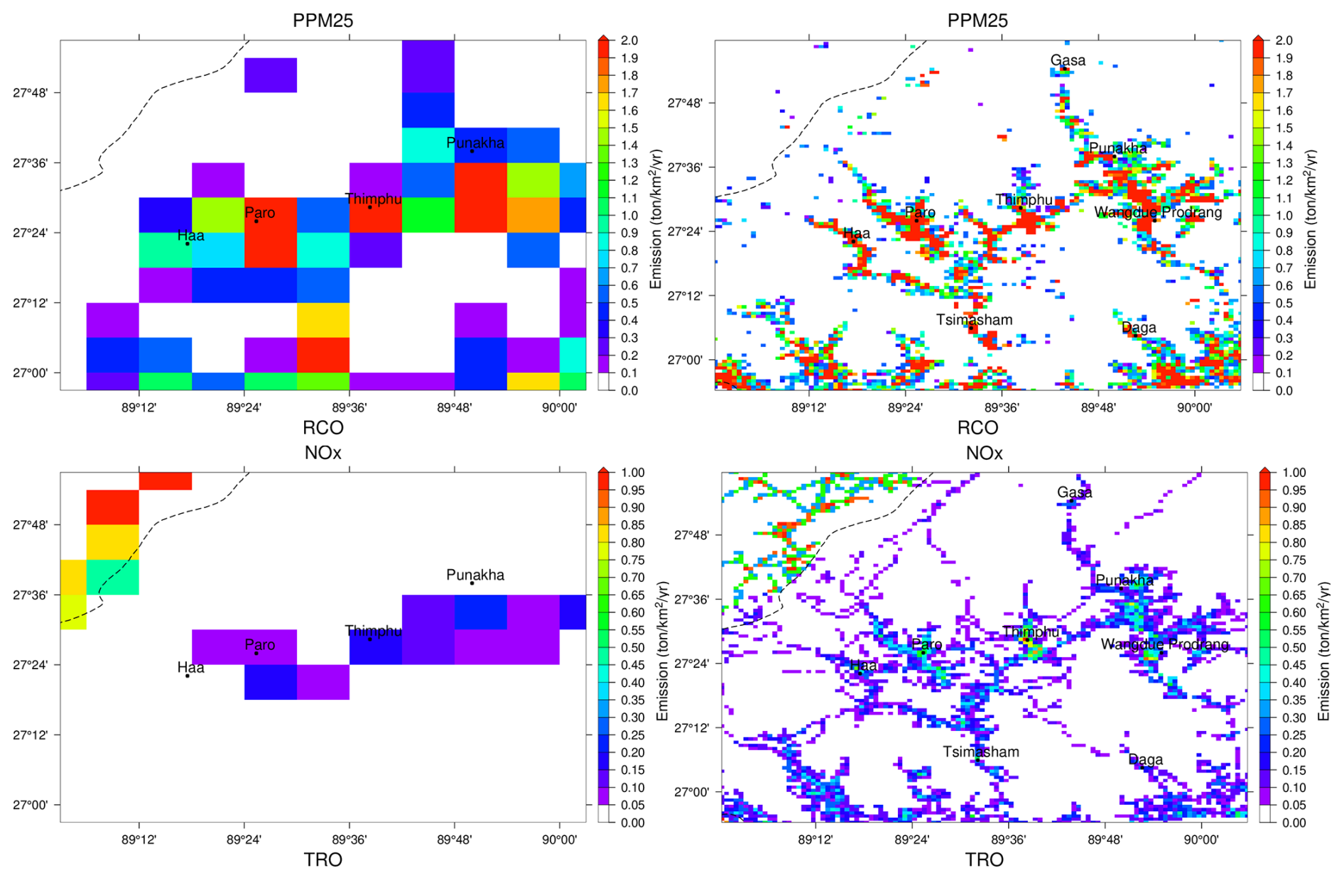
Figure 3 Impact of the downscaling for two species – primary PM_2.5 and NO_x – from low (left) to high (right) resolution for two activity sectors: residential combustion (RCO – top) and traffic (TRO – bottom) over the west Bhutan.

4 Available observations

In Bhutan, there are very few air quality monitoring stations, and only the Thimphu Air Quality Monitoring Station is partially functional. It is currently operated by the Department of Environment and Climate Change, Bhutan, with the support of ICIMOD. The station employs reference-grade (state-of-the-art) equipment’s, including Thermo Scientific (USA) instruments for trace gases (O₃, NO_x, CO, and SO₂), a Grimm (Germany-based) instrument for PM (PM₁₀ and PM_2.5), an Aethalometer (Slovenia) for BC, and Lufft for meteorological data. In the Haa measurement, we have used two AirBeam Low-cost sensors in two different locations (Katsho and Uesu) for PM_2.5. In this study, we have considered the observation data from 20 February to 10 March 2025 for the Thimphu air quality and from 22 February to 26 March 2025, for Haa Valley in Bhutan (Figs. S2–S4). All stations are assumed to be urban or peri-urban background stations i.e. supposed to be not influenced by local sources. Their location is reported in (Table 2). Some meteorological stations have been considered for the evaluation of model performance.

Table 2 Location of stations with observations (air quality and/or meteorology).

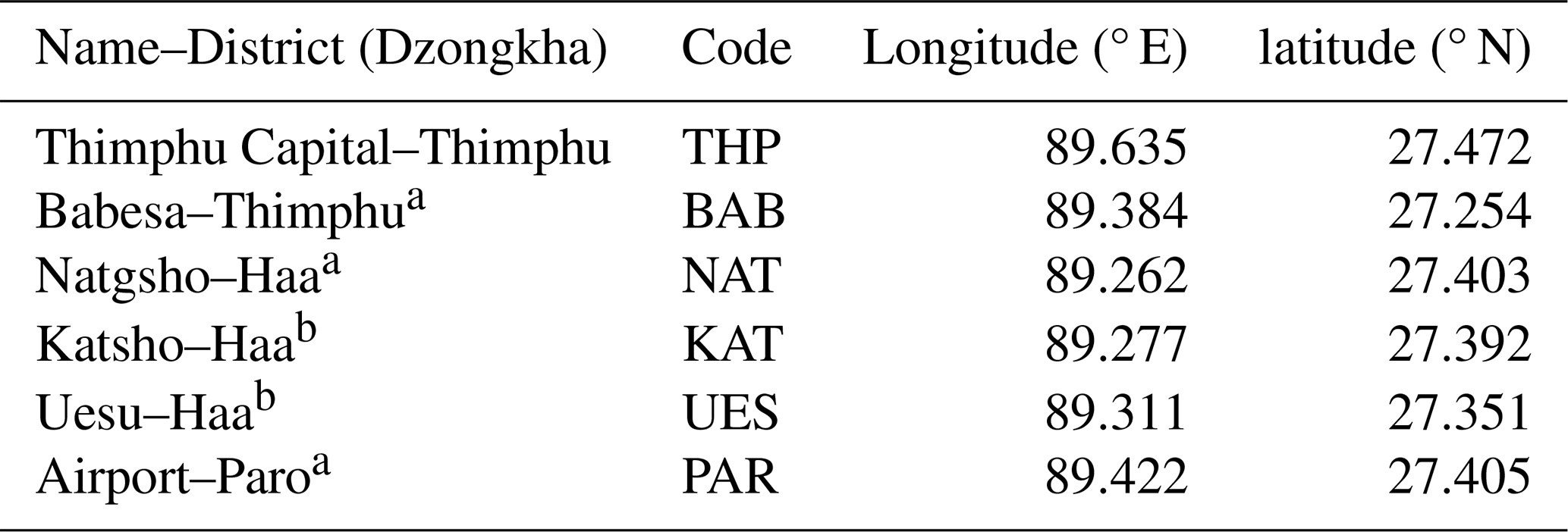
^a Official meteorological stations. ^b Stations equipped with low cost sensors.

4.1 Thimphu (Capital city of Bhutan)

The measurement data show substantial temporal variations in PM and gaseous pollutants. The daily (24 h) concentration of PM_2.5 is consistently above the WHO guideline of 15 µg m⁻³ in Thimphu, with more than double for most of the day. The BC concentration shows that the sharp episodic peaks reach 15 µg m⁻³ and above, with a background concentration below 5 µg m⁻³. The correlation between PM_2.5 and BC is very strong (R²=0.91), which indicates common combustion sources. Hourly PM₁₀ baseline background concentration ranges from 20 to 40 µg m⁻³, and some peaks exceed 100 µg m⁻³. The PM_2.5 concentration shows a similar pattern, but with generally lower values, ranging from 10 to 50 µg m⁻³, with occasional peaks exceeding 50 µg m⁻³.

To explain the large differences sometimes observed between PM₁₀ and PM_2.5 could be related to a missing emission of PM emissions (particularly coarse particles) like road dust resuspension (emissions due to the flow of vehicles). Indeed, in South Asia, outside the monsoon period, the road traffic resuspension is a major source of coarse traffic-related particles. In Delhi, a recent study showed that 79 % of these particles came from resuspension of road dust (Singh et al., 2020). The contribution of non-exhaust PM emissions will get more significant since exhaust emissions will decrease with the renewal of the vehicle fleet and these emissions are not taken into account in models. For the Thimphu station, a very good correlation coefficient of 0.85 exists between the observed PM coarse fraction as $\left({\mathrm{PM}}_{\mathrm{10}}-{\mathrm{PM}}_{\mathrm{2.5}}\right)/{\mathrm{PM}}_{\mathrm{10}}$ with the relative humidity (Fig. 4), by using a quadratic regression. The absolute time correlation reaches 0.96 for the diurnal cycle (Fig. S8). The coarse fraction is correlated (linear regression) with the wind speed with a much weaker correlation coefficient of 0.45 showing that urban resuspension is not the main driver. The relative humidity is therefore a good predictor of the resuspension which is for a urban station likely due to road dust resuspension. Considering the resuspension negligible near 100 %, a remaining 10 % PM coarse fraction is probably due to other anthropogenic emissions. For very low humidity, the coarse fraction of 60 % to 80 % is of the same order of magnitude found by Singh et al. (2020) in Delhi. In addition, Amato et al. (2012) consider that the road dust resuspension also affects the fine fraction, 25 % of re-suspended dust can be considered in the fine fraction.

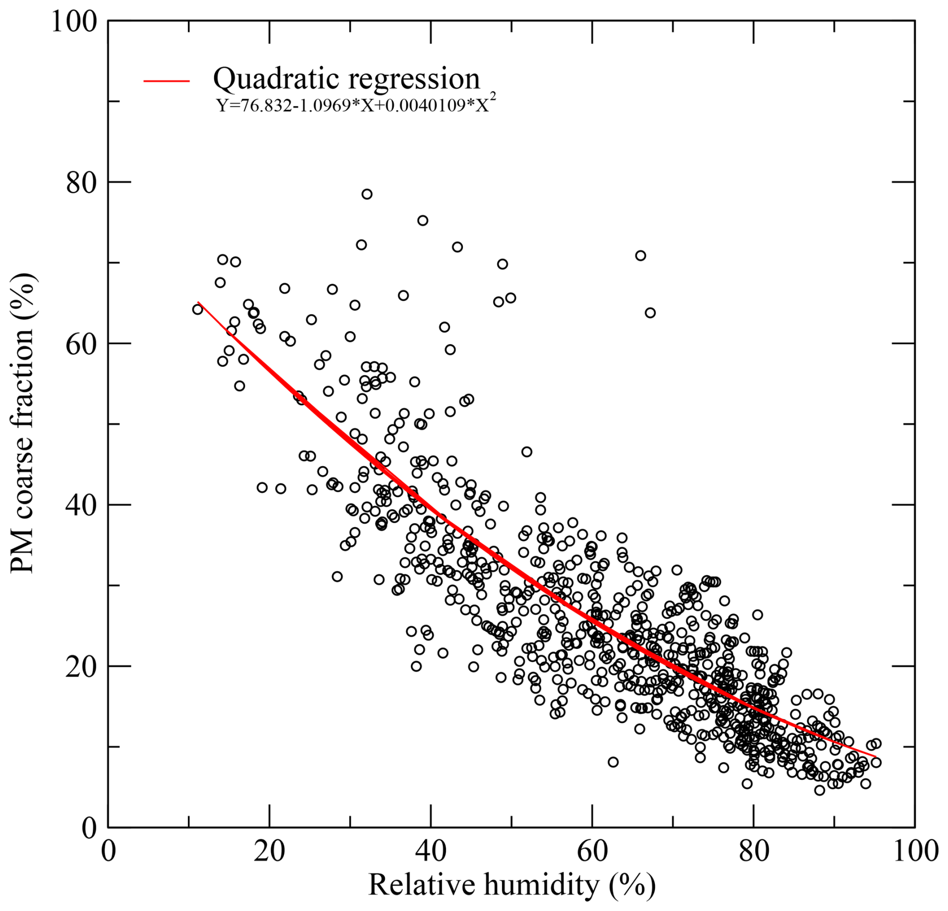
Figure 4 Coarse PM fraction at Thimphu air quality station as a function of relative humidity (circles) and the corresponding quadratic regression (in red).

For Ozone, the running 8 h average maximum concentration remains consistently above the WHO guidelines and the Bhutan National Ambient Air Quality Standard 2020 (51 ppb) throughout the study period, with the exception of one day (28 March). It shows a marked diurnal cycle, with hourly concentrations ranging from 3 ppb at night to 78 ppb in the afternoon. The lowest concentration was observed on 28 February when there was light rainfall, clouds, and no solar radiation. The inverse relationship between the NO_x (NO₂, NO), CO, and O₃ clearly illustrates that the atmospheric reaction and enough precursor compounds are available in the atmosphere (Bhutan) for ozone formation. The NO_x illustrates the distinct diurnal patterns with peaks during the morning (08:00 to 10:00) and evening. The daily variations perfectly align with the high traffic hours patterns. The hourly concentration ranged from 1.5 to about 20 ppb during the measurement periods, and with daily concentration ranged from 3 to 9 ppb. CO concentration displays clear diurnal variability with baseline levels around 200–300 ppb and episodic peaks exceeding 600 ppb. NO_x and CO show a strong temporal correlation (R²=0.88) during the measurement periods, which indicates a significant contribution from common traffic emission sources to the ambient concentrations. SO₂ concentrations are generally low during the monitoring period, typically remaining below 0.6 ppb, with occasional minor peaks. It indicates that no major emission sources for SO₂ are located in the region.

4.2 Haa (High altitude Valley in Bhutan)

The use of Low Cost Sensors (LCS) is common in South Asia (Shabbir et al., 2025) and a hybrid approach with LCS and reference stations is probably the key to improving the air quality monitoring. For Haa, we have used two AirBeam Low-cost sensors developed by HabitatMap in two different locations (Katsho and Uesu) only for PM_2.5. It is a laser-based light scattering optical particle counter technique to measure the PM concentration, temperature, and relative humidity. The instrument records data at intervals of 1 minute in its internal memory. It transmits data via Wi-Fi to a cloud platform for remote access. Before starting the measurements, these sensors are collocated in the Thimphu station, and during data calibration, a correction factor is applied. Based on the measurement, the 24 h average PM_2.5 concentration is consistently higher than the WHO air quality guideline (15 µg m⁻³) throughout the 33 d measurement period. During this period, the daily concentration ranges from 20 to 55 µg m⁻³ in Katsho and from 17 to 57 µg m⁻³ in Uesu. The highest concentrations were recorded from 18 to 21 March at the measurement sites. To evaluate the model, we also used meteorological data measured by the LCS and official stations in Bhutan for the surface temperature (T2M), relative humidity (RELH) and wind speed (WINS).

5 Model performances

Global error statistics (RMSE as Root Mean Square Error, Correlation and bias) on daily data are presented in Table 3, the mean diurnal cycles are displayed in Fig. S5 as well as all time series for all pollutants in Figs. S6 and S7. As in many studies using regional models (Bessagnet et al., 2016) the PM concentrations are underestimated, certainly due to emission inventories which underestimate some emissions like wood burning, a major source in Bhutan that is difficult to estimate. For the PM₁₀ concentrations, the model underestimates the afternoon concentrations with an increase from 14:00 to 16:00 local time while at the same time PM_2.5 does not increase. This behaviour could be due to the missing road dust resuspension process in the model.

Table 3 Spatio-temporal error statistics based on hourly values from 10 February to 31 March 2025 at three resolutions: 0.25° (THP025), 0.05° (THP005) and 0.01° (THP001). The RMSE and bias are expressed in the following units: µg m⁻³ for PM and BC concentrations, ppb for gas concentrations, and °C, %, m s⁻¹ respectively for the 2 m temperature (T2M), relative humidity (RELH) and wind speed (WINS). The last two columns are respectively the averaged observed values (Obs.) and the number of observations (#).

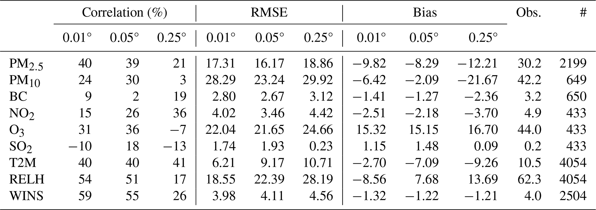
As displayed in Table 3 and Fig. 5, there is clearly an improvement of statistics when we increase the resolution, but from 0.05 to 0.01° we obtain mixed results. Indeed, as mentioned in the literature (Schaap et al., 2015; Colette et al., 2014; Terrenoire et al., 2015), for the concentration of pollutants, increasing the resolution can also produce numerical noise and can degrade some statistics. The largest improvement is obtained from 0.25 to 0.05° however the bias is often at the highest resolution. Valari and Menut (2008) showed for ozone an optimal resolution at about 10 km, which overcomes the problem of uncertainty in wind characteristics at too high resolution when comparing on sparse observational datasets, however this study was performed over the Paris region with a smooth topography. Bessagnet et al. (2020) showed a similar result in a mountainous region with the main improvement from 10 to 3 km spatial resolution for most pollutants with still an improvement from 3 to 1 km on the bias only. For Haa, the model has poor performances for PM_2.5 concentrations which is probably due to more general difficulties to simulate the meteorology in this high-altitude valley and/or the emissions from natural and anthropogenic origins.

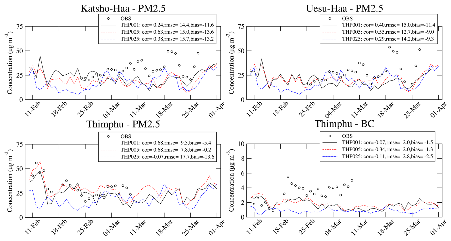
Figure 5 Model versus observations comparisons and error statistics at stations for the three resolutions for PM_2.5 and BC, based on daily values.

For the gases, only observations at the station of Thimphu are available. Ozone concentrations are overestimated, particularly during nighttime (Fig. S5) and certainly a consequence of underestimation of NO₂. It is usual for regional models to overestimate ozone at coarse resolution because of mesh-related numerical effects (Gao et al., 2025). The temporal correlation of ozone is low in the Thimphu station because of a lack of variability in February-March, and the model overestimates the concentrations, particularly at night. The Thimphu station is located not too far from a busy road and some burning activities have been reported explaining the negative bias of the model on BC as well. Indeed, from 19 February a jump of BC concentrations is observed (Fig. 5) due to local sources, while the model was more in line with observations from 10 to 18 February with even a slight positive bias. The diurnal cycle of BC shows the two peaks in the morning and afternoon is respectively shifted in the model by 1 and 2 h.

As already observed in studies using models driven by global emission inventories, it is usual to overestimate sulfur dioxide (Pachon et al., 2024). We remind here that sulfur dioxide concentrations are driven by the industrial and energy sectors, and moreover the high-resolution inventory is downscaled from the gridded EDGAR database. These facilities are typically located outside major urban areas and the proxy used by EDGAR and the downscaling approach could not be adapted, leading to these discrepancies. This has been demonstrated by Thunis et al. (2022) by using a screening approach analysing the inconsistencies that arose on spatial distribution differences for the industrial and energy sectors. As in many global and regional inventories, in our case, the source points are actually merged into surface emission with raw estimates of injection heights based on vertical emission profiles (Bieser et al., 2011).

The simulation of meteorological variables is improved at the highest resolution and particularly for the nighttime temperatures (Fig. S5). Indeed, within the valleys the prediction of the inversion layers and cold pools require an increase in the model spatial resolution (Bessagnet et al., 2020). The wind speed is underestimated during the afternoon, however the diurnal cycle is well captured by the highest resolution simulation. For the relative humidity, the high resolution helps to retrieve the right time of the lowest values in the afternoon.

6 Air pollution and its impact in maps

6.1 Concentrations fields

As mentioned in the introduction, BC is a key component of PM for health and climate concerns, in this section we analyse the spatial patterns of BC and and PM_2.5 (Fig. 6). Over the Indo Gangetic Plain we found values from 2 to 5 µg m⁻³ on average for BC, which is in line with values reported in the literature (Romshoo et al., 2023; Smaran and Vinoj, 2024). The highest values are observed in India and Bangladesh as well as in other big cities like Kathmandu (Nepal). The influence of Delhi (outside the domain) can be observed in the western part of the domain through the monthly climatology used as boundary conditions here.

Figure 6 Average spatial patterns of PM_2.5 and BC concentrations in March 2025 over the Hindu Kush Himalayan region (top) and the West Bhutan (bottom). For the PM_2.5, contour lines represent the percentage of BC in the PM_2.5 (color scales are different for PM_2.5 and BC).

Focusing over Bhutan, the PM air pollution is concentrated within the valleys with a maximum in Thimphu, An other maximum is observed in the south which corresponds to the location of two important cities: Pasakha in Bhutan and Jaigaon in India. This place is a major industrial zone and this hot spot of air pollution is mainly driven by the industrial sectors. Close to the highest PM_2.5 values, the contribution of BC can exceed 5 %. BC concentrations are generally below 1 µg m⁻³ in mountainous sites in line with observations reported in many high altitude stations (Singh et al., 2023). Over the Tibetan Plateau, average BC concentrations are low between 0.1 and 0.3 µg m⁻³ as reported in recent studies (Wang et al., 2024).

In the Himalayan region, the fine fraction is mainly made of Secondary Inorganic species (SIA) and primary carbonaceous species (CARB), the latter species being very dominant in the IGP region, including the south of Bhutan (Fig. 7). Over the north, mineral dust is also the main component where the total PM_2.5 is low, below 5 µg m⁻³. Figure S9 displays the same type of figure for the ultra fine fraction of PM (below 0.1 µm), where SIA largely dominates everywhere, whereas non carbonaceous primary PM dominates (OPPM) in the south of the domain for the coarse PM (diameter between 2.5 and 10 µm). There is no studies looking at the composition at the regional level of PM_0.1 in South Asia. In Europe, Argyropoulou et al. (2025) finds high concentrations of SIA (with high sulfate concentrations due to nucleation) and organics in the ultrafine fraction of PM. In our split of species, organics are split between SOA and CARB categories, with a likely underestimation of secondary production since in our chemical mechanism the production of SOA from the emitted organic aerosol was not activated. This assumption is supported by recent studies in India (Panda et al., 2025; Bhattu et al., 2024) showing the chemical production of secondary organics from biomass burning and traffic emissions.

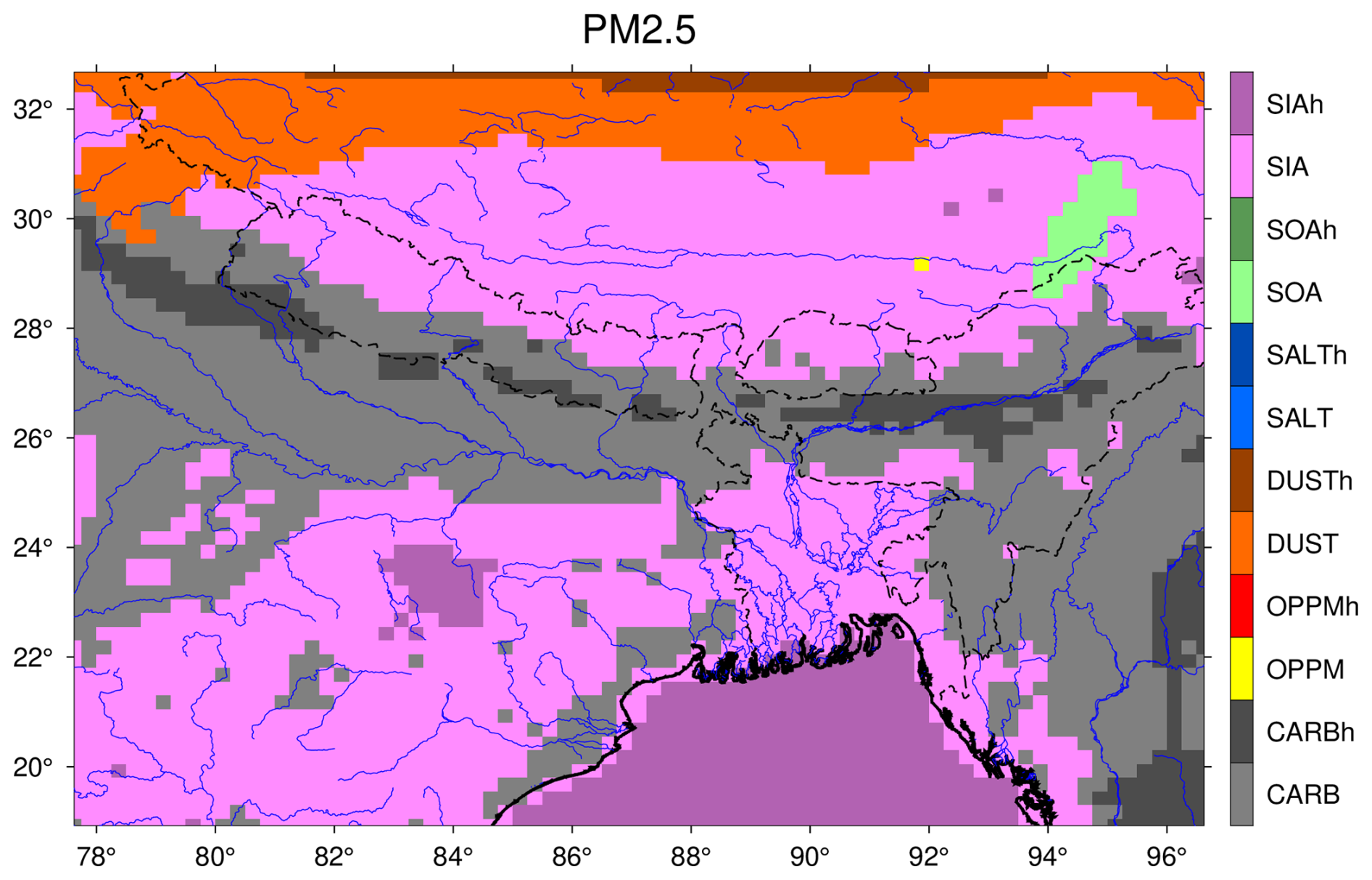
Figure 7 Average dominant components in the fine fraction of PM (PM_2.5) over the widest domain THP025 in March 2025. Macro species are named as CARB (BC and primary OM), OPPM (other mineral primary anthropogenic species), DUST (mineral desert dust), SALT (sum of sodium and chloride), SOA (Secondary Organic Aerosol) and SIA (Secondary Inorganic Aerosol as the sum of nitrate, sulfate and ammonium). Suffix h mentions when the dominant species concentration is at least twice the second most important component.

6.2 Deposition spatial patterns

The cumulative total deposition for the following list of macro species are displayed in Fig. 8 for the month of March 2025:

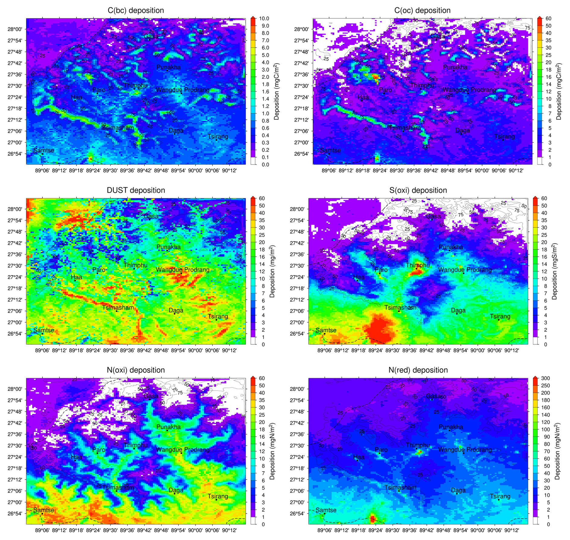
Figure 8 Spatial patterns of total deposition in March 2025 over the highest resolution domain THP001 at 0.01°. The contour lines show the wet deposition fraction (25 %, 50 % and 75 %).

• N(red). total reduced nitrogen species: ammonia (NH₃) and ammonium (NH₄⁺),

• N(oxi). total oxidized nitrogen species: NO_y as NO + NO₂ + HNO₃ NO${}_{\mathrm{3}}^{-}$ and other PAN species (Peroxyacetyl nitrate),

• S(oxi). total oxidized sulfur species: sulfur dioxide (SO₂) and sulfate (SO₄²⁻),

• C(bc). carbon from black carbon,

• C(oc). carbon from the organic matter issued from primary species (mainly wood burning and wildfires here),

• Dust. from mineral dust emissions (here transported from boundaries of the domains).

Carbon from the secondary organic species is excluded in C(oc) to mainly target the role of wood burning and wildfires.

6.2.1 Carbon and mineral dust

One of the most significant light-absorbing substances causing the atmosphere to warm is black carbon (BC). After its release into the atmosphere from the burning of fossil fuels and biomass, BC can settle on distant glacier surfaces and hasten glacier melting, leading to increased negative mass balances of glaciers and diminished freshwater supplies downstream (Li et al., 2023, 2021; Réveillet et al., 2022; Lapere et al., 2023). Therefore, when researching the climatic effects of BC in the atmosphere and in the glacier regions, it is crucial to take into account three key links: BC and mineral dust emissions from source regions, transport, and deposition in remote glacier regions. The darkening of snowy surface is probably underestimated by chemistry transport models if the Brown Carbon (BrC), a fraction or Organic Matter mainly emitted by biomass burning, is not well taken into account in models (Chelluboyina et al., 2024). There are also evidence in the literature that mineral dust has a strong impact on glacier melting (Chandel et al., 2025), and even could dominate the darkening of glaciers through the long-range transport of dust after sand and dust storms.(Sarangi et al., 2020). Therefore, it is of major importance to also track the primary fraction of the organic matter as a good tracer of the BrC. In our study, over our domain covering the West Bhutan, we observe that the primary carbon deposition fluxes are mainly due to organic matter – C(oc) – largely emitted by biomass burning (Fig. 8 and Table 4). Then, BrC deposition fluxes in Bhutan are probably higher than for BC. Over the highest mountain of the domain close to the border with China (Jomolhari peak), total BC deposition ranges from 100 to 300 µg m⁻² in March, while C(oc) deposition is 10 times higher from 1 to 2 mg m⁻². Gul et al. (2024) found a monthly rate of BC dry deposition close to 140 µg m⁻² using another regional model for another Himalayan glacier in the Himalaya (Yala in Nepal) which is coherent with our results and probably overestimated as stated by the authors. It is also important to better understand what we call BC in emission inventories, whether it is BC (based on optical measurement) or Elemental Carbon as EC (based on thermal methods). At emission BC is probably higher than EC and after ageing in the atmosphere and depending on the mixing state of particles, Carbon could have different optical properties (Liu et al., 2022; Zhang et al., 2023). We also must differentiate which fraction of carbon comes from biomass burning to be treated as BrC with less absorbing optical properties. In the air pollution community, these clarifications are crucial.

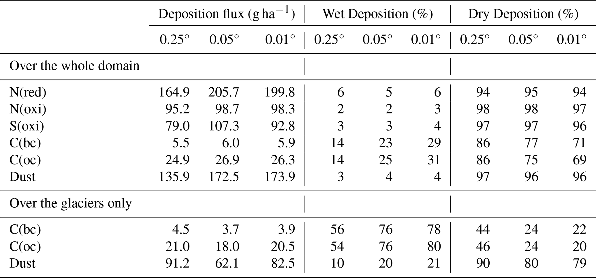
Table 4 Impact of the horizontal resolution on the average deposition flux simulated by CHIMERE of key species – N(red), N(oxi), S(oxi), C(bc), C(oc) and dust – over the highly resolved domain THP001 at 0.01° resolution. Last rows are average values of deposition fluxes focusing on the glaciers and perpetual snows for C(bc), C(oc) and dust.

Regarding dust, similarly to the findings of Sarangi et al. (2020), dust deposition is much larger than black carbon deposition and will have an impact on the glacier melting (Fig. 8 and Table 4). For our simulation, there are no emissions of dust in our domains and, overall, the fraction of wet deposition over total deposition is below 5 % for the period of interest. Therefore, all deposited dust comes from outside the domains through a complex interaction of vertical mixing processes within the boundary layer involving mountain breeze, sedimentation and then deposition over forested areas and over the glaciers as well. From the southwest side of the domain, the long-range transport of dust in the free troposphere above 4000 m a.s.l. impact first the higher hills stretching from Tsimasham to the North-West (see Fig. 8). The cross-section in Fig. 9 shows dust transport from the southwest to the northeast of the finer domain on a given daye in March. It shows high-altitude dust transport around 5000 m in the early morning, which later mixes downward as the planetary boundary layer develops. These findings highlight the importance of including dust, BC, and BrC when assessing the impact of air pollution on glacier melting.

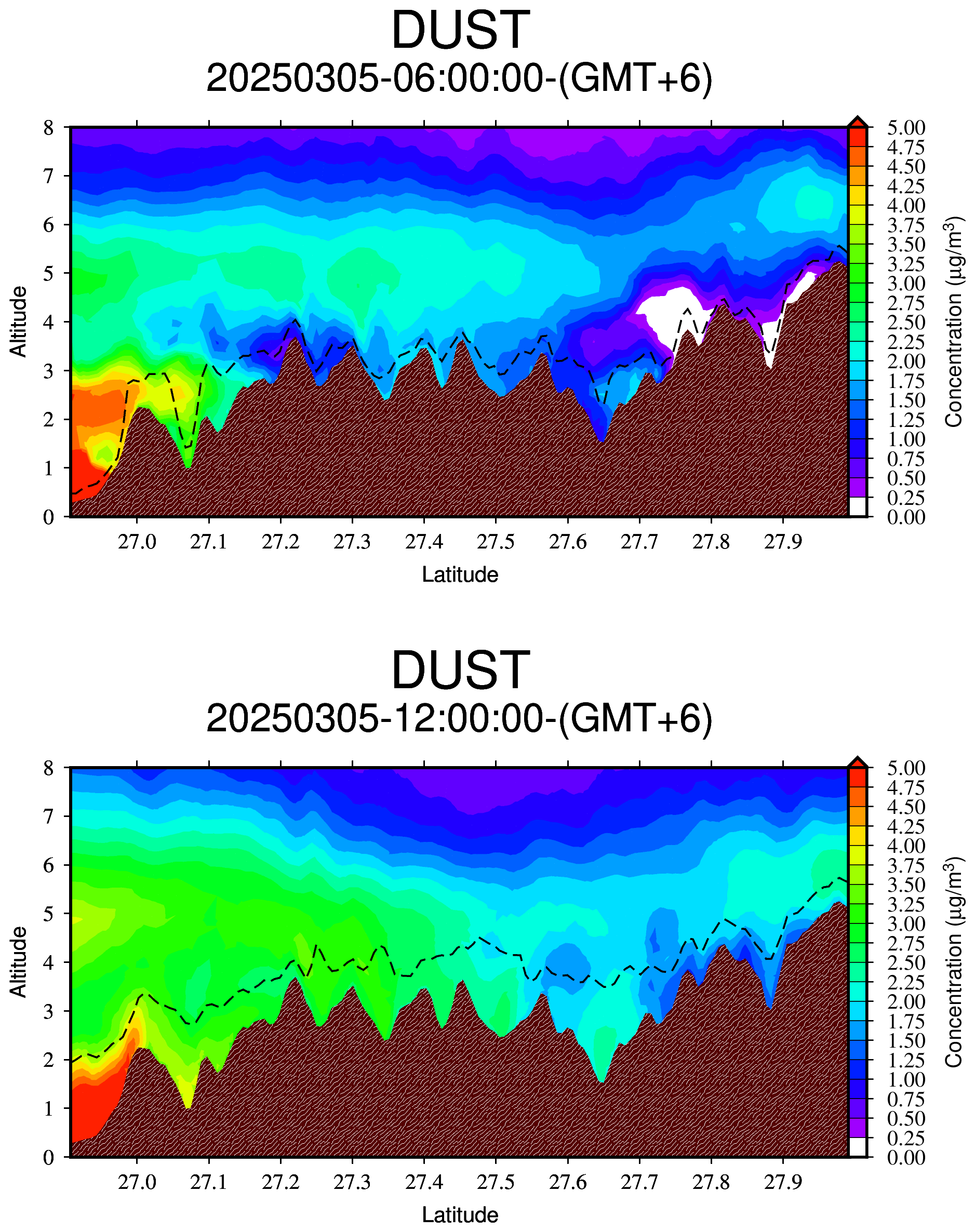
Figure 9 Vertical cross section of dust concentrations from the Southwest to the Northeast over the THP001 domain (89° E–26.9° N to 90.15° E–28° N) the 5 March 2025 at 06:00 GMT+6 (top) and 06:00 GMT+6 (bottom). The dash-line represents the average height of the planetary boundary layer.

Focusing on deposition over the glaciers and perpetual snows (last rows of Table 4), the deposition fluxes for carbonaceous species have the same order of magnitude as for the whole domain but the fraction of wet deposition is much larger showing the importance of wet deposition over the glaciers due to precipitations and a less efficiency of dry deposition over bare soils. For dust, the deposition fluxes are twice lower over the glaciers compare to the average value over the whole domain but it remains comparable.

6.2.2 Inorganic species (Sulfur and Nitrogen)

From large scale models at low resolution, the global picture of ammonia patterns shows that South Asia is a hot spot (Pai et al., 2021; Xu et al., 2018). Very few data exist over the Himalayan region regarding the deposition of inorganic species like reduced and oxidized nitrogen species. Nearby, in East Asia, a network monitors the acid deposition and air pollution (UNEP and ACAP, 2025). Wang et al. (2023) have reconstructed a positive trend of ammonium deposition over the Tibetan glaciers since 1950 but a slight decrease since 1990 probably due to changes of atmospheric circulations. Using the isotopic composition of nitrogen, Bhattarai et al. (2019) showed that the air contamination from South Asia to the Himalayan Tibetan Plateau is very likely impacting the high altitude ecosystems. A most recent and exhaustive study has been performed by Ellis et al. (2022). They first evaluated published literature defining nitrogen thresholds (critical levels and loads) at which lichen epiphytes are impacted. Second, to characterize model variability, they employed estimates from previously published atmospheric chemistry models up to 10 km resolution projected to the Himalaya with different spatial resolution and timelines.

We find that nitrogen reduced species deposition dominates with values close to 50 mgN m⁻² accumulated in March 2025 (Fig. 8). For oxidized nitrogen values are slightly lower between 10 and 30 mgN m⁻². The south of the domain centered in West Bhutan as well as the valleys are the most affected, however even if agriculture is not the major source of ammonia in Bhutan, the reduced nitrogen can be transported over very long distance as ammonium in particles and can be then deposited very far from the primary ammonia emission. The average value of the total deposition flux of nitrogen for the month of March 2025 (around 300 gN ha⁻¹ on average as reported in Table 4) is of the same order of magnitude with a critical value estimated by Ellis et al. (2022) at 4.24 kgN ha⁻¹ yr⁻¹ for the Himalayan region. According to the deposition fluxes displayed in Fig. 8 (sometimes exceeding 100 mgN m⁻² i.e. 1 kgN ha⁻¹ for one month) this annual threshold is likely to be exceeded in the South of Bhutan. However, this needs to be assessed with a proper calculation of the critical loads with an annual simulation. Indeed, A critical load requires the use of models using (i) soil chemistry (buffering capacity, base saturation), hydrology (water flow, retention) and vegetation sensitivity. For Europe, deposition values of more than 1 kgN ha⁻¹ yr⁻¹ were simulated by Vivanco et al. (2017). As elsewhere in the world, deposition of oxidized sulfur is lower than the deposition of total nitrogen compounds. The highest values are located in the south of the domain over the most industrial areas.

In Table 4 is highlighted the effect of the spatial resolution (0.25, 0.05 and 0.01°) on the total deposition flux for each species computed over the finest domain THP001 focused on West Bhutan. While the calculation of deposition is properly done by looping over each land use, we calculate the fluxes over the glaciers as a post-treatment by considering only the location of glaciers and their surface fraction in each cell. Chemistry transport modelling involved various non-linear processes, the main being the chemical production of species like ozone and secondary inorganic PM (like ammonium nitrate). Moreover, the landuse fraction and the meteorology changing with the change of resolution will imply a difference on the calculation of deposition fluxes. Finally, accumulating over one month, the difference on the total amount is not so important considering all these non-linearities and input data variability.

However, oxidized sulfur and reduced nitrogen species look the most affected by the resolution since they are involved ina very non-linear process where the spatial resolution will play an important role. For instance, the sulfur chemistry depends on the pH in clouds which is affected by the resolution where clouds can not be diagnosed in a coarse grid while they could be formed at a finer grid. In March, dry deposition dominates the total deposition which is normal during this post-winter period with low recorded precipitation amounts. The wet deposition increase with an increase of resolution, as the consequence of an increase of precipitation with higher resolution simulations (30 % more precipitation in THP001 compared to THP005). The wet deposition fraction is significantly higher for carbonaceous species than for inorganic species. It means that these carbonaceous species are probably emitted close to the location affected by precipitation. Inorganic species are emitted and formed close to more urbanized or industrialized areas father away from remote places.

7 Evaluation of the wildfire contribution to air pollution

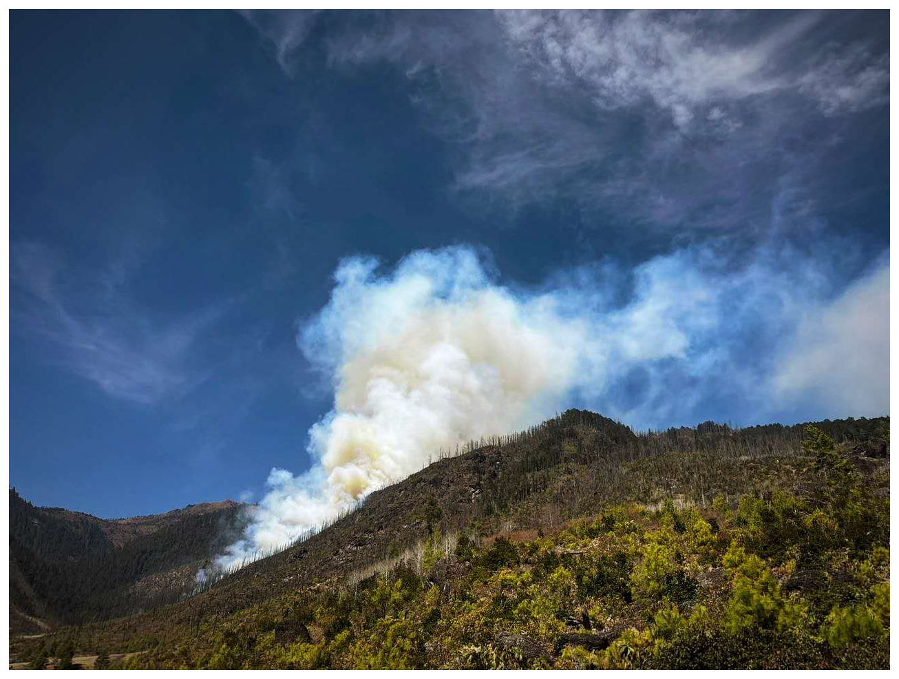
Biomass burning is known to have an impact up to the Tibetan Plateau (Li et al., 2016). Wildfires are observed in the north of Haa and Paro districts (Dzongkha) during three main periods in March 2025: 6–8, 17–21 and 26–31 (Fig. 10). Wildfires were confirmed by VIIRS Fire and Thermal Anomalies available from the NOAA-21 satellite (NASA VIIRS Land Science Team, 2020) as shown in Figure S10. For the first period, the wildfire started at a middle distance between Paro and the Jomolhari peak and the 3D video supplement (powered by VAPOR – Sgpearse et al., 2023) based on CHIMERE outputs shows a potential impact up to the glaciers surrounding the peak at concentration lower than 1 µg m⁻³.

Figure 10 Wildfires observed nearby Haa on 21 March 2025 (credit: Tenzin Wangchuk).

A combination of several processes makes the transport of BC possible: (i) the daytime anabatic flows along the valley, (ii) the increase of the planetary boundary layer, and (iii) finally, the concentrations are cleared by a strong synoptic southwesterly flux. Unfortunately, we do not have ground or satellite observations to confirm this feature. As shown in Fig. S11, Bhutan is often covered by clouds over the north making the retrieve of Aerosol Optical Depth almost impossible most of days. For the last period, we performed a numerical simulation to highlight the role of forest fires over the West of Bhutan. In Fig.  11, we compare the PM_2.5 concentration between a case without fires over the three domains (NOFI) and the reference simulation with wildfires (CTRL) over a 10 d period 17–31 March 2025. The difference [CTRL−NOFI] can then be considered as the contribution of wildfires.

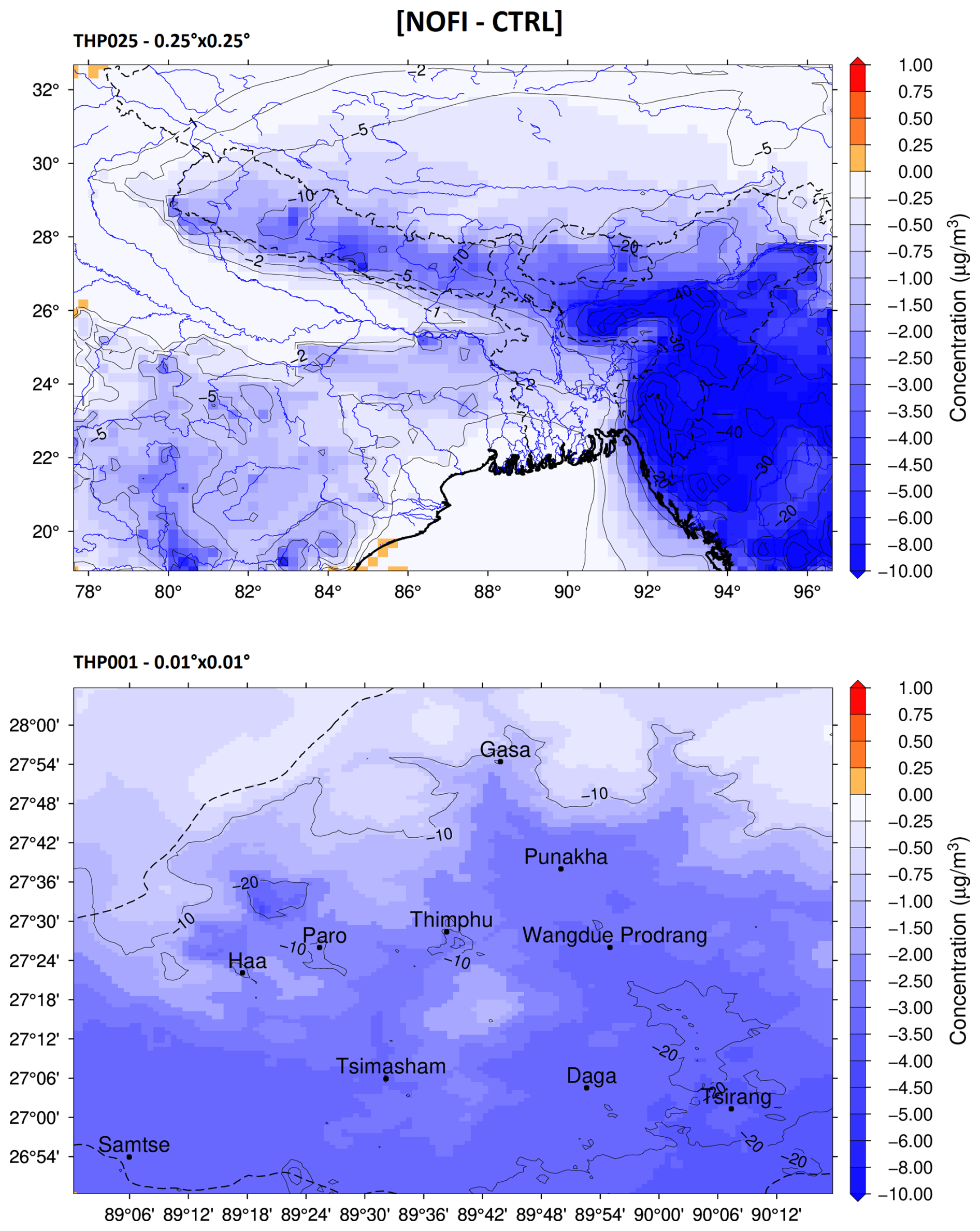
Figure 11 Impact of fires on PM_2.5 concentrations for the THP025 and THP001 domains (respectively top and bottom). Average concentration decrease without fire emissions over all domains (NOFI – CTRL) from the 17 to 31 March. The contour lines are the reduction in % (from the CTRL reference case concentration)

Over the widest domain, we observe that the main impact is located over the East part of the domain in Myanmar and East India (states of Assam, Meghalaya, Manipur, Mizoram and Nagaland). These regions are usually affected by wildfires in spring and particularly in March and April before the monsoon season (Unnikrishnan and Reddy, 2020). In this location, fires contributes to more than 40 % of PM_2.5 in line with findings of Kumari et al. (2024). In the Hindu Kush Himalaya region, Nepal and Bhutan are the most affected and it is only the start of the fire season for these countries. Over the West Bhutan, the local fires in Haa and Paro district contribute locally to up to 20 % of PM_2.5 on average over the 15 d period. This average value hides large time variability with sometimes hourly contributions exceeding 70 µg m⁻³ at close to wildfire emission sources. The contribution of fires issued from Myanmar and India can be observed in the South-East border of Bhutan with a relative contribution of 20 % thanks to south-easterly winds. Removing fires also reduces other gas emissions, leading to small potential increases over north due to due to chemical non-linearities, the slight increase of PM is mainly due to some increase of sulfate formation without fires over some places in India and over the Indian Ocean. The sulfur chemistry and sulfate formation is influenced by the oxidant capacity and the pH of cloud droplets, then a small change can positively or negatively modify all chemical processes slight increase of sulfate. Thus, it is not surprising to observe the strongest changes over the ocean where the relative humidity is high and where sulfate is also emitted by sea salts and produced from the Dimethyl sulfide.

Wildfires can contribute up 10 %–20 % during some hours at Katsho. The contribution is mainly driven by carbonaceous species (black carbon and organic matter). Interestingly, all statistics are improved when fires are taken into account, with a slight improvement of time correlation, 0.60 and 0.66 respectively for NOFI and CTRL simulations. Wildfires have also an influence on ozone, NO₂, sulfate and nitrate concentrations (Fig. S12). Overall, without fire emissions the concentrations are impacted by up to −10 ppb in the east part of the wider domain THP025. This indirect impact is due to the NO₂ emission reductions without wildfires in a NO_x-limited region (low NO_x concentrations). Far from wildfire sources, NO₂ concentrations can even slightly decrease. The chemistry is actually changed over the whole domain and in some place the oxidant capacity can be slightly enhanced when the fire emissions are not taken into account. Because of specific chemistry regimes (due to titration by NO_x), an increase of ozone is rarely observed over the North of India leading in this region where the presence of megacities leads sometimes to VOC-limited regimes. In Bhutan, a decrease of 1 to 2 ppb is observed. This region has low NO₂ concentrations and is mainly NO_x-limited, and a decrease in Volatile Organic Compounds and NO_x emissions due to wildfires will automatically reduce ozone concentrations.

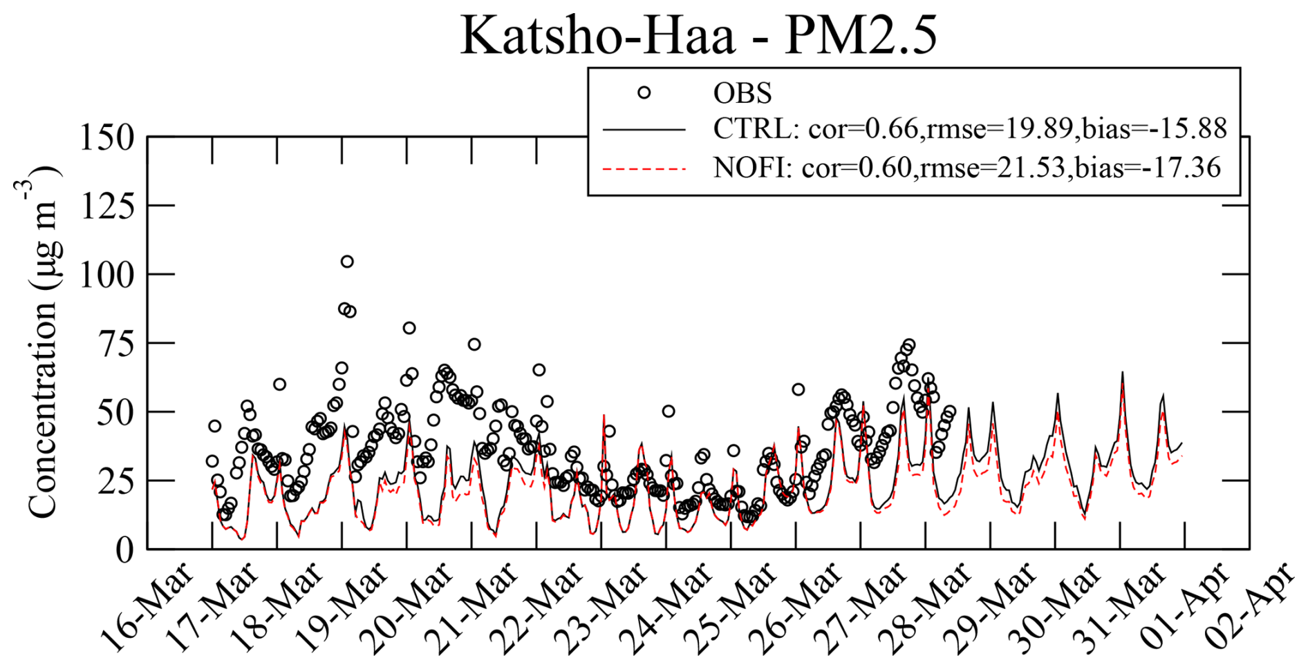
Figure 12 Timeseries in UTC time of PM_2.5 concentrations for the CTRL reference simulation and the simulation without fires (NOFI) against observations.

8 Conclusions

For the first time, an air quality simulation at 1 km horizontal resolution over Bhutan has been performed with the regional chemistry transport model CHIMERE over a large domain covering several Himalayan valleys. The model was run over a period after the winter season (beginning of February to the end of March 2025) to benefit from additional measurements in the Haa valley with two low cost sensors. The simulations highlight the issue of air quality in Bhutan valleys with an important contribution of carbonaceous species to the level of PM_2.5 concentrations that largely exceed the WHO guidelines. From the analysis of the simulation outputs, we can draw the following additional conclusions:

• increasing the spatial resolution improves the model performances on meteorological variables and air pollutant concentrations in urban areas, but improvements of the spatialisation is still needed particularly for industrial sources,

• road dust resuspension must be considered in models as it is an important fraction of coarse particles but also fine particles, particularly in South Asia,

• cumulative total deposition fluxes in March 2025 over the finest domain at 0.01° of key species over the month of March 2025 are consistent through the three spatial model resolutions with similar simulated values,

• the simulated patterns of deposition fluxes confirm the potential role of dust, BC and probably BrC on glaciers melting and the capacity of the model to simulate the impact of air pollution,

• our simulations confirm that Himalayan forests are expected at risk from excess nitrogen, the levels of deposition fluxes calculated in March are comparable to high values computed or observed in many other locations worldwide,

• wildfires can have a strong impact in the valleys of Bhutan, their contribution to PM_2.5 concentrations can exceed averaged values of 20 % during the outbreak of fires and Bhutan can also be affected from fires occurring in North-East India and Myanmar.

At this point, a model setup to simulate air quality is available. The model has been run over a limited temporal window which is the main limitation of this study. Additional studies and applications can be carried out to monitor air pollution and create the most effective measures for enhancing air quality in the Himalayan valleys. This study is an opportunity to highlight the need to have a more comprehensive modelling framework to study the impact on glaciers accounting for dust and the carbon from the Black and Brown Carbon, this latter been driven by biomass burning sources that are important in the Himalayan valleys. For PM_2.5, it is also important to create a network of low-cost sensors in the Hindu Kush Himalaya to monitor both indoor and outdoor air pollution, complementing a set of reference stations. Increasing the resolution will be helpful to evaluate the effect of air pollution on glaciers, ecosystems, and human health including social aspects. Then, using cutting-edge machine learning techniques, models will be used in combination with measurements to get an exhaustive picture of air pollution in the region and participate to the necessary dialogues between all the countries in the Hindu Kush Himalaya. As a last point, we suggest that the creation of a high resolution emission inventory with a bottom-up approach should be a priority of the regional institutions responsible for air quality management.