On the Weather Impact of Contrails: New Insights from Coupled ICON–CoCiP Simulations

Contrail forecasts typically neglect feedbacks with the atmosphere. Here, we couple the Contrail Cirrus Prediction model (CoCiP) with the global Icosahedral Non-hydrostatic (ICON) numerical weather model in a two-way mode accounting for contrail-weather interaction. The models exchange atmospheric and contrail state variables after each time step using the coupler YAC. ICON includes a new two-moment cloud ice microphysics scheme that enables skillful predictions of ice supersaturation. CoCiP now limits the uptake of ambient ice supersaturation when many contrails form. Radiation is calculated in ICON using the ECMWF radiation scheme ecRad. Contrail radiative forcing is computed from the difference of ICON results with and without contrail feedback. The coupled system results are broadly consistent with offline CoCiP simulations. The ICON results are validated against radiosonde observations and compared with ECMWF forecasts showing improved score values. The significance of the computed contrail effects is tested by numerical noise perturbation or twin experiments comparing the results of forecast pairs with initial values differing randomly. Contrails induce a butterfly effect with disturbances growing with time. Contrails induce disturbances similar to random disturbances. Within the first 5 d, contrails warm the ambient air at contrail levels. Contrails change the surface temperature and precipitation locally by an order 1 K and 10 mm d⁻¹, with pattern similar to random disturbances and with magnitude depending on ambient weather, with negligible global mean changes. After 5 d, the weather changes are dominated by the butterfly effect. The slow response of the surface temperature to contrail RF deserves further investigations.

1 Introduction

Much has been learned since the 1990's about the formation of condensation trails (“contrails”) (Schumann and Heymsfield, 2017; Kärcher, 2018). Contrails form behind aircraft burning hydrogen or hydrocarbon fuels in sufficiently cold air (Schumann, 1996). Contrails persist in ice supersaturated ambient air (Minnis et al., 1999; Spichtinger et al., 2003; Haywood et al., 2009). Contrails have similarity to moderately thin cirrus (Liou, 1986; Hong et al., 2016), causing a radiative forcing of climate change by scattering part of the incoming solar radiation back to space and reducing outgoing terrestrial radiation (Meerkötter et al., 1999; Wolf et al., 2023). Globally, the latter effect dominates causing a positive mean radiative forcing at top of the atmosphere and warming below the contrails in the troposphere (Ponater et al., 2005; Burkhardt and Kärcher, 2011; Schumann and Mayer, 2017). Hence, contrails from global aviation are considered to contribute to global climate change on Earth (IPCC, 1999; Sausen et al., 2005; Lee et al., 2021; Teoh et al., 2024b; Bickel et al., 2025).

The climate impact of contrails can be reduced by optimizing flight routes such that the formation of warming contrails gets minimized (Teoh et al., 2020; Martin Frias et al., 2024). Such optimization requires reliable high-resolution weather forecasts and an efficient and accurate contrail model, besides accurate aircraft and flight route data. Several studies have assessed the limited accuracy of weather forecasts with respect to predicting the conditions for contrail formation (Gierens et al., 2020; Hofer et al., 2024; Wang et al., 2025). But it is unknown so far how strongly weather forecasts change when the feedbacks of contrails are included.

Here we investigate the impact of contrails on weather by coupling the contrail model CoCiP (Schumann, 2012) with the global Icosahedral Non-hydrostatic numerical weather prediction model ICON (Zängl et al., 2015).

CoCiP was originally developed as an offline contrail model that uses atmospheric conditions provided by a climate or numerical weather prediction (NWP) model. In this offline mode, contrails evolve (grow and decay) within the given environmental conditions without influencing them. This approach introduces a bias in cirrus cloud lifetimes because it neglects the feedback whereby contrails reduce ice supersaturation, as shown in climate models (Burkhardt and Kärcher, 2011; Schumann et al., 2015). The coupled ICON–CoCiP model developed for this study allows to forecast contrails interacting with the background atmosphere and allows us to investigate and quantify this feedback with respect to weather forecasts.

The ICON model is based on a non-hydrostatic numerical integration scheme on an icosahedral grid with nearly uniform spatial resolution globally. The model has been extended by a new two-moment cloud ice microphysics scheme replacing the operational one-moment cloud ice scheme with a prognostic cloud ice-number density and explicit ice nucleation. The concept has been described by Köhler and Seifert (2015). The extension was necessary to model ice supersaturation which is essential for contrail persistence.

Weather can be predicted for several days, but the predictability decreases with forecast time, partly because of the growth of small uncertainties in the initial conditions (Bauer et al., 2015). From detailed large eddy simulations, we know that contrails change the atmosphere in its immediate environment (Jensen et al., 1998a; Unterstrasser and Gierens, 2010; Lewellen, 2014; Unterstrasser, 2016). We also know that contrails change the mean state of the atmosphere at climate time scales (Schumann et al., 2015; Bock and Burkhardt, 2016; Gettelman et al., 2021). Do contrails change weather forecasts at time scales of a few days significantly? Or are initial changes dominated by the butterfly effect (Lorenz, 1969; Zhang et al., 2003; Rotunno and Snyder, 2008; Selz et al., 2019)? It seems that this has not been investigated so far.

The data exchange between ICON (running on several parallel computing processors) and CoCiP (running on a single processor) is accomplished in a two-way (2-way) mode using Yet Another Coupler (YAC), a coupling method that has been developed to couple Earth system models, such as atmosphere and ocean model components (Hanke et al., 2016). After each ICON time step, CoCiP obtains the data from ICON, see Fig. 1, integrates the contrail changes and returns the contrail properties affecting the weather state, both via the coupler.

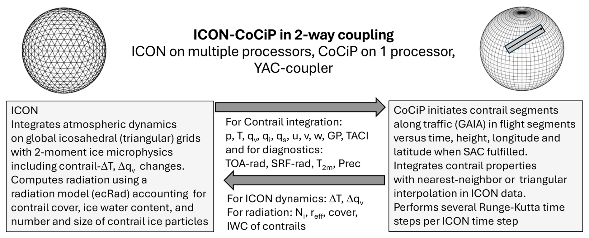
Figure 1 ICON–CoCiP coupling concept. From ICON: p: pressure (in Pa); T: temperature (K); q_v, q_i, q_s: mass fractions of water vapor, ice and snow (kg kg⁻¹); u, v, w: wind velocities (easterly, northerly, and upward, in m s⁻¹); GP: geopotential (m² s⁻²), TACI=τ_cirrus: solar optical depth of cirrus clouds above given height (1); TOA-rad, BOA-rad: top of atmosphere and bottom of atmosphere (surface) downward radiation fluxes (W m⁻²); T_2 m: temperature at 2 m height above ground (K); Prec: total precipitation amount at the surface (m). From CoCiP: ΔT, Δq_v: temperature and humidity changes by contrails (K and kg kg⁻¹), Ni: number of ice particles in the contrail (1 kg⁻¹), r_eff: effective contrail ice particle radius (m), contrail cover (m² m⁻²), IWC: contrail ice water content (kg kg⁻¹).

In order to better understand predictability and the sensitivity in the atmospheric system to contrails it has been recommended to use perturbation experiments to assess the evolution of differences within model simulations (Ancell et al., 2018). Here, the significance of the computed contrail effects is tested by comparison to numerical noise perturbation or twin experiments.

This paper gives a short description of the methods and some of the tests performed, and then presents the results of simulations of 10 d forecast initialized from four selected dates covering winter and summer conditions. More extensive simulations over longer periods remain to be done in the future. Hence, the paper discusses the short-term effects of contrails on weather.

2 Methods

The atmosphere is computed using the global Icosahedral non-hydrostatic (ICON) model and contrails with the Contrail Cirrus Prediction Model (CoCiP). For analysis of contrail effects on the state of the atmosphere and its development over a few days (“the weather”), ICON and CoCiP are run either in the “1-way mode” or in the “2-way mode”, see Fig. 1. In the 1-way mode, ICON simulates the reference state, i.e., the state of the atmosphere without contrails, and CoCiP uses the ICON output as obtained via YAC after each ICON time step, together with traffic data from the Global Aviation emissions Inventory based on ADS-B (GAIA) (Teoh et al., 2024a), to compute the contrail properties. In the 2-way mode, CoCiP obtains the ICON output and computes the contrail properties as before and returns the changes in humidity and temperature as well as the radiatively relevant contrail properties per ICON grid cell via YAC to ICON.

For testing the significance of the contrail-induced weather changes we run the coupled code for four forecasts starting 00:00 UTC 1 January, 25 June, 15 July and 15 December 2021, covering winter and summer conditions. The June and July cases were studied experimentally within the HL-CIRRUS experiment (Jurkat-Witschas et al., 2025). The variance of the contrail induced weather changes in the simulations for four different days over the year is taken as one of the measures for assessing the uncertainty of the mean values for these forecasts.

In addition, we perform a twin experiment. A twin experiment compares two ICON simulations starting from initial values that differ by small disturbances of temperature, humidity, and horizontal and vertical wind, similar to round-off errors. Here one of the two runs uses disturbances by random factors (1+ε) multiplying each field of the initial values, where ε are small numbers with root-mean-square (rms) amplitude of 10⁻¹², differing randomly for each grid cell and each field. We also performed such runs with 10⁻¹⁴ and 10⁻¹⁰ amplitudes; ICON computes in double precision implying round-off errors of the order 10⁻¹⁵. For studying the impact of random disturbances in the ICON fields on CoCiP results, the twin experiments are also run with CoCiP in the 1-way mode. For the ICON variables, the undisturbed 1-way simulation is used as control simulation. For small ε, the twin experiment provides a lower bound on atmospheric error growth. Comparing the 2-way coupled simulation that includes the effect of contrails with the twin control experiment allows causal interpretation of model differences. Any systematic difference between the 2-way coupled simulation and the twin control runs – beyond the natural divergence between the twin control experiments – may be attributed to contrail-related forcing.

2.1 The ICON model for simulating the global atmosphere

The ICON model used for this study simulates the atmosphere at 120 vertical grid layers covering heights between 0 and 75 km above ground. A subset of 41 levels covers the ICON levels between about 5.2 and 18.4 km height, sufficient for analysis of contrails in the upper troposphere and lower stratosphere. The vertical grid resolution is 300 m uniformly between 4.3 and 14 km height, increasing above and decreasing below, with 20 m near ground. The model can be run with fine and coarse horizontal resolution, with 737 280 or 2 949 120 triangular grid cells, and 26.6 or 13.3 km mean grid scale. The cloud microphysics uses the so-called advective time step of ICON, i.e., 240 or 120 s. Internally, the dynamics uses a smaller time step with iterative sub-stepping (Zängl et al., 2015). Ten-day simulations are performed with the coarse grid; three-day simulations with either fine or coarse grid. The model can be initialized with either DWD or European Center for Medium-Range Weather Forecasts (ECMWF) Integrated Forecasting System (IFS) initial conditions. Here we report results using the IFS initial conditions. Radiation fluxes are computed using the ecRad radiation solver of the ECMWF (Hogan and Bozzo, 2018).

ICON provides three-dimensional (3d) fields to CoCiP characterizing the state of the atmosphere after each ICON time step, including p, T, q_v, u, v, w and τ_cirrus (see Fig. 1). In addition, two-dimensional (2d) data fields are provided defining the radiative fluxes at TOA (outgoing longwave radiation OLR, solar direct radiation SDR, and reflected solar radiation RSR) and corresponding downward and upward shortwave (SW) and longwave (LW) radiation fluxes at the Earth surface, together with T_2 m, the temperature at 2 m height above the surface, and PREC, the time-integrated precipitation amount since forecast start.

ICON was equipped with a 2-moment microphysics scheme to simulate the cloud ice extending the operational 1-moment cloud ice scheme with a prognostic cloud ice-number density and explicit ice nucleation (Köhler and Seifert, 2015). The ice particle sources considered are homogeneous and heterogeneous ice nucleation and detrainment of cloud ice. Homogeneous ice nucleation simulation follows Kärcher et al. (2006) for grid-scale ice supersaturation and for the given vertical velocity. The model for heterogeneous ice nucleation uses the ice nucleating active sites (INAS) parameterization of Ullrich et al. (2017). For details see Hanst et al. (2025). The ICON version used is free of any stochastic parameterizations or random parameters during the model integration.

Special care was needed to handle the following issues: (1) In the microphysics model, cirrus clouds form as soon as the ambient humidity exceeds the threshold for ice saturation. However, contrails are often observed to persist in otherwise cloud-free ice-supersaturated air masses (Jensen et al., 2001; Ovarlez et al., 2002; Schumann, 2002; Thompson et al., 2024). (2) Most radiation schemes, including the ecRad version used in ICON, represent ice clouds with a single category characterized by a bulk effective radius. This can introduce nonlinear artifacts when coexisting clouds are present. This happens for instance, when optically thin natural cirrus with large particles and full cloud coverage (cloud fraction=1) coexist with contrails, which typically feature high in-cloud ice water content (IWC), small particles, and low cloud fraction. (3) In numerical weather prediction (NWP) models, it is common practice to exclude very thin, subvisible ice clouds from the calculated cloud cover when calculating radiation transfer. This approach better aligns with both human observations and the limitations of most remote sensing instruments, which often have a detection threshold. As a result, only optically significant ice clouds are considered in radiation schemes. However, when assessing the radiative impact of contrails, the treatment of subvisible cirrus becomes important.

To address these issues, ICON employs a subvisible cirrus correction. For the two-moment cloud ice scheme, this is implemented using an optical-depth threshold for cirrus visibility of τ_ext=0.02, which corresponds, for an extinction efficiency Q_ext=2 and an ice density ${\mathit{\rho }}_{\mathrm{i}}=\mathrm{950}\mathrm{kg}{\mathrm{m}}^{-\mathrm{3}}$, to a dynamic ice water content threshold

$${\text{IWC}}_{\text{crit}}={\displaystyle \frac{A}{\sqrt{N_{\mathrm{i}}\mathrm{\Delta }{z}^{\mathrm{3}}}}}\text{with}A={\displaystyle \frac{\mathrm{4}{\mathit{\tau }}_{\text{ext}}^{\frac{\mathrm{3}}{\mathrm{2}}}{\mathit{\rho }}_{\mathrm{i}}}{\mathrm{3}{\mathit{\pi }}^{\frac{\mathrm{1}}{\mathrm{2}}}{Q}_{\text{ext}}^{\frac{\mathrm{3}}{\mathrm{2}}}\mathit{\rho }}}\approx \mathrm{0.714}.$$

Here, N_i is the ice particle number density in m⁻³, Δz is the vertical grid spacing in m, and ρ is the ambient air density. If the IWC of a cirrus layer is below this threshold, its cloud fraction C is reduced according to $C_{\text{reduced}}=min(C,\text{IWC}/{\text{IWC}}_{\text{crit}})$. Without this limit, far more thin cirrus clouds would arise. In this study, cirrus clouds within ice-supersaturated regions (ISSRs) that have a cloud fraction C_reduced<5 % are excluded from the radiation calculation. This prevents nonlinear artifacts that could otherwise bias the estimation of contrail radiative forcing. Importantly, these adjustments affect only the radiation scheme; the microphysical processes in ICON remain unchanged. Hence, this formulation provides a consistent treatment that minimizes, but cannot entirely eliminate, inconsistencies arising from the limitations of ICON. Of course, the results depend on details of this approach which were selected after some sensitivity studies. A more physically consistent solution would require, for example, the use of spectral bin microphysics and multiple ice categories in the radiation scheme. While this is, in principle, possible within ICON, it is not employed in the current study.

2.2 The CoCiP model for contrail simulations

CoCiP is a Lagrangian model which traces individual contrails segments forming between waypoints along flight routes for many flights, globally. CoCiP first reads the traffic data for the given time step interval and computes newly formed contrail segments based on the Schmidt–Appleman Criterium (SAC) (Schumann, 1996). Then it follows the contrail segments moving with the wind and with the contrail crystal's mean fall speed in the ambient atmosphere. The modelled contrail ice content accounts for growth of the contrail plume with time by turbulent mixing and exchange of humidity with the ambient air and is computed assuming ice saturation inside the contrail plume. For each contrail waypoint, the model keeps the local time, longitude, latitude, pressure altitude, ambient temperature, and humidity and the properties of the subsequent segment, including length, depth, width and skewness of the assumed Gaussian contrail plume cross section, contrail mass per length, mass specific ice water content, number of ice particles per flight distance, optical depth of the contrail and optical depth of cirrus above the contrail.

The traffic data are obtained from GAIA with a time resolution of about 40 s. They include the flight id and aircraft type, the segment lengths, the coordinates of the segment endpoints, and the aircraft performance (mass, true air speed, fuel consumption, overall propulsion efficiency, soot emission index), computed using an open-access performance model (Poll and Schumann, 2025). The traffic data are read hourly and provided internally with interpolated end points for each integration time interval.

The fields characterizing the state of the atmosphere are obtained by CoCiP from ICON via the YAC coupler after each ICON time step. CoCiP keeps the data for the actual weather state and for the state one timestep earlier for linear interpolation of contrail properties for any time within the recent ICON time step interval (120 or 240 s). The ambient conditions are computed at contrail waypoints by interpolating in the gridded fields, with pressure according to flight levels (ICAO, 1964), with linear interpolation vertically and in time, and by nearest neighbor or linear interpolation horizontally in the triangular ICON grid. At start of the program, the grid geometry (grid cell coordinates, geopotential level heights, cell area and volume) is specified and a precomputed table is used defining the four closest grid cells for a set of discrete latitude–longitude coordinates globally with 0.125° resolution. This table defines the three grid cell centers with closest distance to a set of discrete longitude–latitude positions which are used for linear triangular interpolation horizontally. The nearest neighbor grid cell value at each discrete point gives nearly the same contrail results with less computing time but with some stepwise horizontal variability of the contrail properties.

The properties of new contrail segments and of contrail segments formed earlier are integrated in time using a second-order Runge–Kutta scheme with time steps of 60 s. After each time step, CoCiP diagnoses statistics including total fuel consumed and mean contrail properties, and checks for contrail persistence.

The 3d fields impacting radiation are added to the ICON cirrus fields, linear for ice water mass fraction $\text{IWC}={\text{IWC}}_{\mathrm{1}}+{\text{IWC}}_{\mathrm{2}}$ and linear for the number of ice particles per mass $N=N_{\mathrm{1}}+N_{\mathrm{2}}$ (here, indices 1 and 2 for contrails and cirrus). For the cloud cover per grid cell area C we follow Hogan and Illingworth (2000) and assume so-called random overlap (defined without random numbers) of contrails and cirrus clouds: $C=C_{\mathrm{1}}+C_{\mathrm{2}}-C_{\mathrm{1}}\times C_{\mathrm{2}}$, keeping $\mathrm{0}\le C\le \mathrm{1}$. The effective radius (r) of the ice particle contrail-cirrus mixture is computed from

$$r={\displaystyle \frac{r_{\mathrm{1}}^{\mathrm{3}}\times N_{\mathrm{1}}+r_{\mathrm{2}}^{\mathrm{3}}\times N_{\mathrm{2}}}{r_{\mathrm{1}}^{\mathrm{2}}\times N_{\mathrm{1}}+r_{\mathrm{2}}^{\mathrm{2}}\times N_{\mathrm{2}}}}$$

as for spherical particles (Hansen and Travis, 1974; Schumann et al., 2011), with the effective radius r_eff=0.9r_vol of contrail ice derived from the volume mean radius computed as in earlier CoCiP versions. The same relationships are used inside CoCiP when collecting grid cell mean contrail properties from the contributions of all contrail segments within the grid cell.

The original CoCiP model simulates contrails, segment by segment, assuming no interaction between neighboring contrails. This assumption does not account for sharing ambient humidity between various contrails when the contrails coincide or overlap each other in the same ICON grid cell. Here we found that the coupled ICON–CoCiP model occasionally gets unstable when many thick contrail segments take up more humidity than available in the related grid cell of ambient air. Therefore, CoCiP was extended with a control field to monitor the amount of supersaturation per grid cell. The control field is filled at start of the timestep with the mass of humidity above ice-saturation per grid cell available in the ambient air before contrails form. During integration of the contrail ice mass, the control field gets reduced (or increased) by the mass of ice taken up (or sublimated) by a contrail segment in the grid cell, and the ice formation is set to zero when this field gets zero. The control fields at the ends of a given time-interval are linearly interpolated to intermediate times. We also tested iterative methods to avoid a stepwise change in humidity uptake, but such iterative methods require far more memory and computing time without changing the results strongly.

In the past, some CoCiP applications run the model with a limit for the vertical contrail depth (Teoh et al., 2024b). We found (see results below) that this limit becomes obsolete after limiting the vertical and horizontal plume diffusivities to maximum values of 10 and 100 m² s⁻¹, respectively, consistent with observations (Schumann et al., 1995) and large-eddy simulations (Dürbeck and Gerz, 1996).

CoCiP computes an estimate for the top-of atmosphere (TOA) shortwave (SW), longwave (LW), and net (SW + LW) radiative forcing (RF), based on a parametrization of libRadtran results (Mayer and Kylling, 2005; Schumann et al., 2012). The CoCiP-computed RF is used for diagnostics of 1-way simulations. In the 2-way coupling, the contrail RF is computed with the ICON-internal radiation transfer model by taking the difference between the simulation results with and without contrails.

Triggered by the comparison of CoCiP with ICON-ecRad (Sect. 3.4 below), we checked whether the model possibly underestimates the nonlinearity in the dependency of RF on the solar optical thicknesses of the contrail and other cirrus above the contrail. In the course of this work, we setup a unified table of the libRadtran results for all 8 considered ice particle habits, which was unpublished so far. Then, a check of the old model (“version 1”) fit revealed changes in the model coefficients only at the level of round-off errors. So, the original model is correct and fully consistent with libRadtran data. However, we created a new model (“version 2”), with three more terms for SW and one more term for LW RF, to allow for a stronger nonlinearity of the dependencies on the optical thicknesses. A test for a uniform cirrus layer is presented below and the data and details are described in Schumann (2025). All other results are computed using version 2.

CoCiP is coded in Fortran-90 in a modular structure with care for efficient loop vectorization, keeping the data of aged contrails in core storage, and is operated by run-scripts organizing the ICON–CoCiP coupling via a namelist, in combination with ICON and YAC namelists. Running CoCiP on a single processor is of course not the best solution. However, implementation of CoCiP on multi processors is difficult because of the Lagrangian treatment of contrail segments moving with the wind, implying that some of them need to be transferred from one processor to another one. A run in which the contrail movement was test-wise suppressed, results in far thicker contrails because the contrails then come into contact with fresh ambient air not yet depleted from ice supersaturation by the contrail in the past.

3 Test Results

3.1 Comparison with radiosonde and ECMWF IFS data

An important feature of the ICON model is its capability to provide realistic values of the relative humidity over ice, RHi. This property is fundamental to simulate persistent contrails and often discussed when comparing alternative forecast models (Gierens et al., 2020; Teoh et al., 2022; Thompson et al., 2024; Hanst et al., 2025). The ICON results show realistic maximum RHi values of about 1.9 in the coldest air masses (below 190 K) near the tropopause in winter. The relative humidity with respect to liquid water stays below about one (maximum value found: 1.004) and is largest in the lower troposphere.

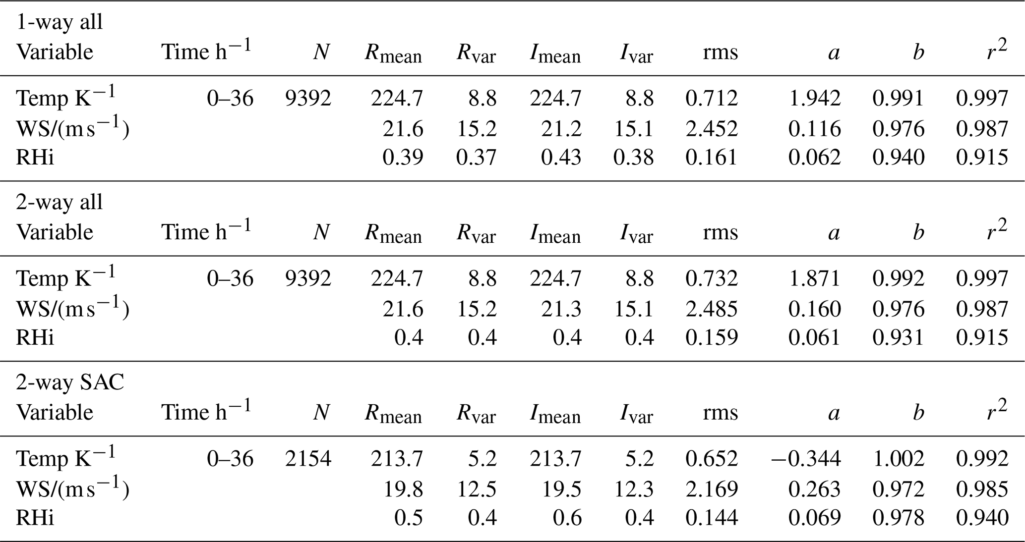
For a quantitative assessment, we present comparisons to RS41 Vaisala radiosonde sensors (Sun et al., 2019) from the DWD data archive, covering mainly northern midlatitudes, and compare with forecast results from the ECMWF IFS model (without contrails) (Tompkins et al., 2007; Bauer et al., 2015). The radiosondes measure the GPS position, relative humidity over water, absolute temperature, horizontal wind speed and direction, and pressure versus time with 1 s time resolution while rising at typically 6 m s⁻¹ speed. The data do not provide the measured relative humidity but the equivalent dewpoint temperature. The dewpoint temperature is converted to water vapor partial pressure using the liquid water saturation pressure function used by Vaisala (Hyland and Wexler, 1983; Vömel et al., 2007). The relative humidity over ice is computed with the ice saturation pressure function as used in ICON (Hanst et al., 2025). When comparing radiosonde data with IFS forecasts we use the IFS ice saturation pressure function. The ICON (and IFS) data are interpolated to the actual time-dependent positions of the radiosondes. For comparison, the data are averaged over 20 hPa pressure intervals between 500 and 120 hPa. The comparisons include the radiosonde data in the first 36 h after forecast start, and cover either all ambient conditions or only those ambient conditions which are cold enough to let contrails form according to the SAC for kerosene, including cases with zero propulsion efficiency, e.g., for idle flight during descent.

The results, see Fig. 2, show considerable scatter, indicating deviations between the ICON model and the radiosonde observations, in particular for RHi. The differences between 1-way and 2-way mode calculations are small compared to the variances and therefore not shown. Noteworthy, the scatter gets reduced, as also reflected in the statistics, see Table 1, when restricting the comparison to cases in which the SAC is satisfied, both in the observed and modelled values. The Pearson correlation r² decreases slightly for temperature and windspeed when reducing the data set according to the SAC criterium, which is to be expected because of the smaller data range. Hence, the increase in the r² for RHi is even more important.

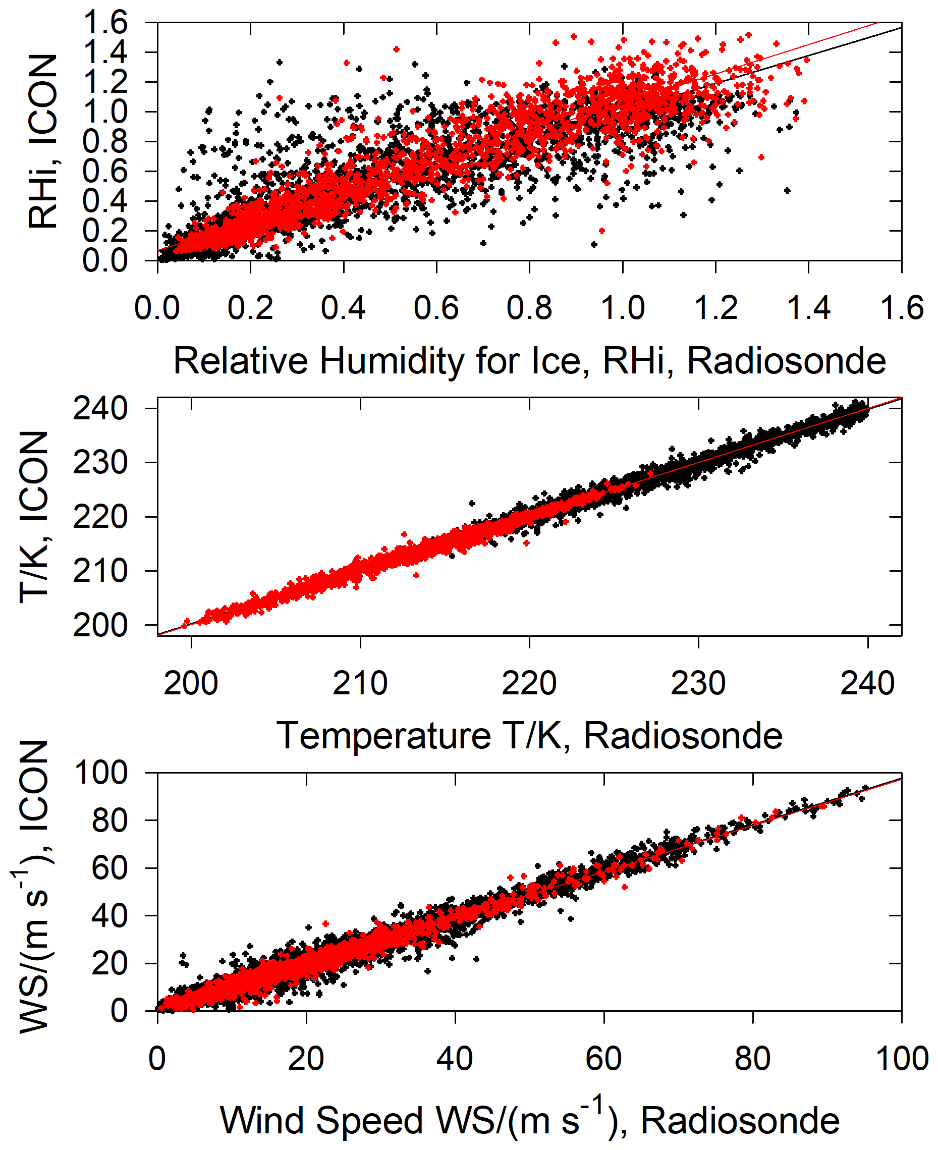
Figure 2 Correlations between Radiosonde observation data and ICON model results (coupled with CoCiP in the 2-way mode) on fine grid for relative humidity with respect to ice (RHi), temperature (T), and windspeed (WS). Black symbols: for all conditions between 120 and 500 hPa (about 5.6–17 km) height. Red symbols: for conditions when the SAC is satisfied. For correlation statistics see Table 1. The red correlation line in the top panel indicates that the ICON RHi values are about 5 % higher than the radiosonde data in the analysis for SAC satisfied.

Table 1 Comparison of ICON results with radiosonde measurements for relative humidity RHi, temperature T, and windspeed WS, first for 1-way and then for 2-way coupling, first for all data and then for data satisfying the SAC. Listed are the time: forecast period; N: number of data points; R_mean and R_var: mean value and variances of radiosonde results; I_mean and I_var: corresponding ICON results; linear regression results zero-value a and slope b; quadratic Pearson correlation coefficient r²; and the rms value of the radiosonde observations (averaged over 20 hPa intervals from 120–500 hPa) and corresponding ICON simulation results.

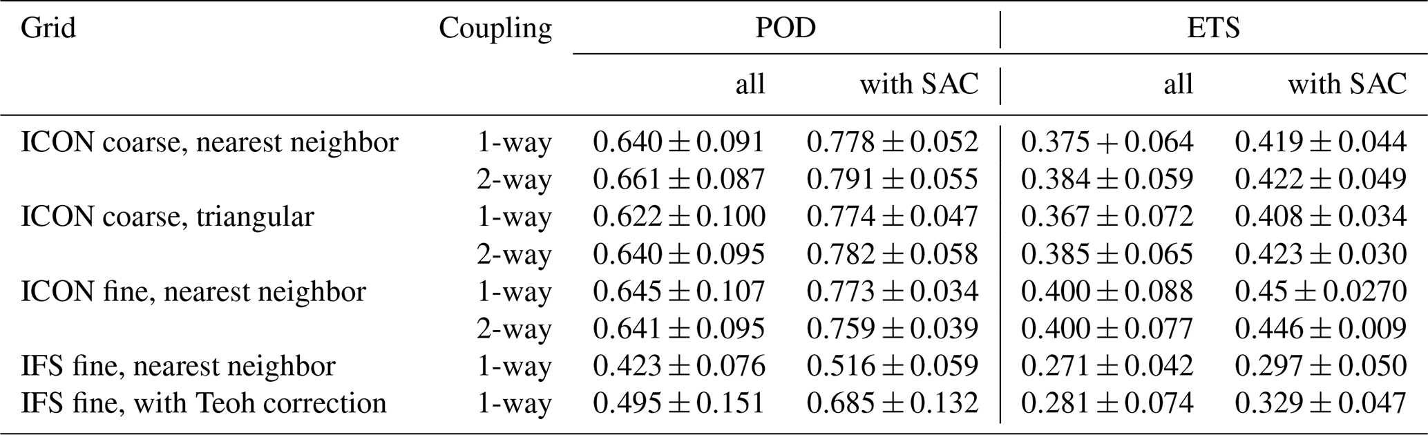
The performance of the ICON model in various versions has been further tested and compared to that of the IFS model based on often used Probability of Detection (POD) and Equitable Threat Score (ETS) scores derived from contingency tables for RHi>1 or <1, from observations and model predictions (Hogan et al., 2010; Gierens et al., 2020; Driver et al., 2025; Hanst et al., 2025), see Table 2. The differences between ICON results for nearest neighbor and triangular interpolation are insignificant. All ICON scores are clearly better than the IFS scores, mainly because of higher ice supersaturation values. We see improved IFS scores when the IFS RHi values get corrected as suggested by Teoh et al. (2024b), in particular in cases where the SAC is satisfied, but the changed IFS scores still stay below the ICON score values. The model-radiosonde agreement improves slightly when running ICON on the fine grid instead of the coarse grid. Noteworthy, the mean correlations between measured and modelled RHi improve from about 0.92–0.94 when using the 2-way mode instead of 1-way mode in the ICON–CoCiP coupling, which may indicate that the coupling to CoCiP improves the ICON weather predictions. However, the results for the fine grid do not support this finding, perhaps because of the limited statistics. Overall, the high scores are mainly due to the improved ice microphysics in ICON, as shown by Hanst et al. (2025).

Table 2 Probability of Detection (POD) and Equitable Threat Score (ETS) values for RHi predictions for 36 h by ICON in 1-way and 2-way modes, with coarse and fine grid, with nearest neighbor and linear triangular interpolation, and by IFS on an octahedral reduced Gaussian grid with 137 vertical layers, 2560 latitude lines between the poles and 6 599 680 discrete grid points globally (about 0.07° resolution), in the pressure interval 120–500 hPa, with the truth assumed to be given by the radiosonde data, either for all data or for data for which the SAC is satisfied only. The IFS results are also analyzed after applying the humidity correction suggested by Teoh et al. (2024b). The mean and rms values are derived from the results for four forecasts days. The POD and ETS are defined as $\text{POD}=\text{TP}/(\text{TP}+\text{FN})$ and $\text{ETS}=(\text{TP}-r)/(\text{TP}+\text{FN}+\text{FP}-r)$, where $r=(\text{TP}+\text{FP})\times (\text{TP}+\text{FN})/(\text{TP}+\text{FP}+\text{FN}+\text{TN}$), with counts TP for true positive (RHi>1 observed and predicted), TN (RHi<1 observed and predicted), FP for false positive (RHi<1 observed and RHi>1 predicted) and FN for false negative (RHi>1 observed and RHi<1 predicted).

On average, the model results agree with the radiosonde data when the SAC is satisfied with rms values below about 0.7 K, 2.2 m s⁻¹ and 0.14 for temperature, wind speed and RHi, and with high contingency scores POD>0.79, ETS>0.42. The model results for mean RHi are about 4 %–8 % higher than the measured values. This tendency is also seen in the correlation plot (top panel of Fig. 2) and revealed by the positive start of the linear regression lines (coefficient a in Table 1). It is hard to decide whether this is due to measurement or modelling issues. For a few hours flight of the research aircraft HALO during CIRRUS-HL at 5–13 km height over Germany on 25 June 2021 (Jurkat-Witschas et al., 2025), passing the tropopause, we compared the in-situ measurements with the ICON data. The results show no systematic RHi bias, supporting the model results for this case. In other model studies the modelled RHi values were often significantly below the measured values (Teoh et al., 2022). So, with ICON, we can run the contrail simulations without artificially adapting the humidity values.

The correlations r² were also computed separately for six 6 h-windows (details not shown) enclosing the radiosonde release times from 3–9, 9–15 h, etc., until 33–39 h after initialization, showing a weak time dependence: The temperature correlations stay near 0.995±0.03, the wind correlations stay near 0.990±0.05, while the humidity correlations decrease slightly from 0.93–0.91 with increasing forecast time.

Still, one may ask how it could be that a radiosonde measures RHi values near 0.1 while the ICON data show RHi near 1, or vice versa, as to be seen in Fig. 2. Figure 3 depicts a typical sounding for such a case with extreme RHi differences. We see that large differences occur near inversions like the tropopause. As shown by the correlation plot insert in that figure, the humidity differences are correlated with temperature differences. Moreover, the humidity differences occur often together with large wind differences. The (modelled) vertical wind is often low in such situations, so related microphysics effects alone do not explain the humidity differences. We also run a few tests with DWD instead of IFS initial conditions and found that the results with IFS initial conditions perform better. Hence, accurate model initial values and accurate numerical integration schemes are at least as important as a high-quality ice microphysics model.

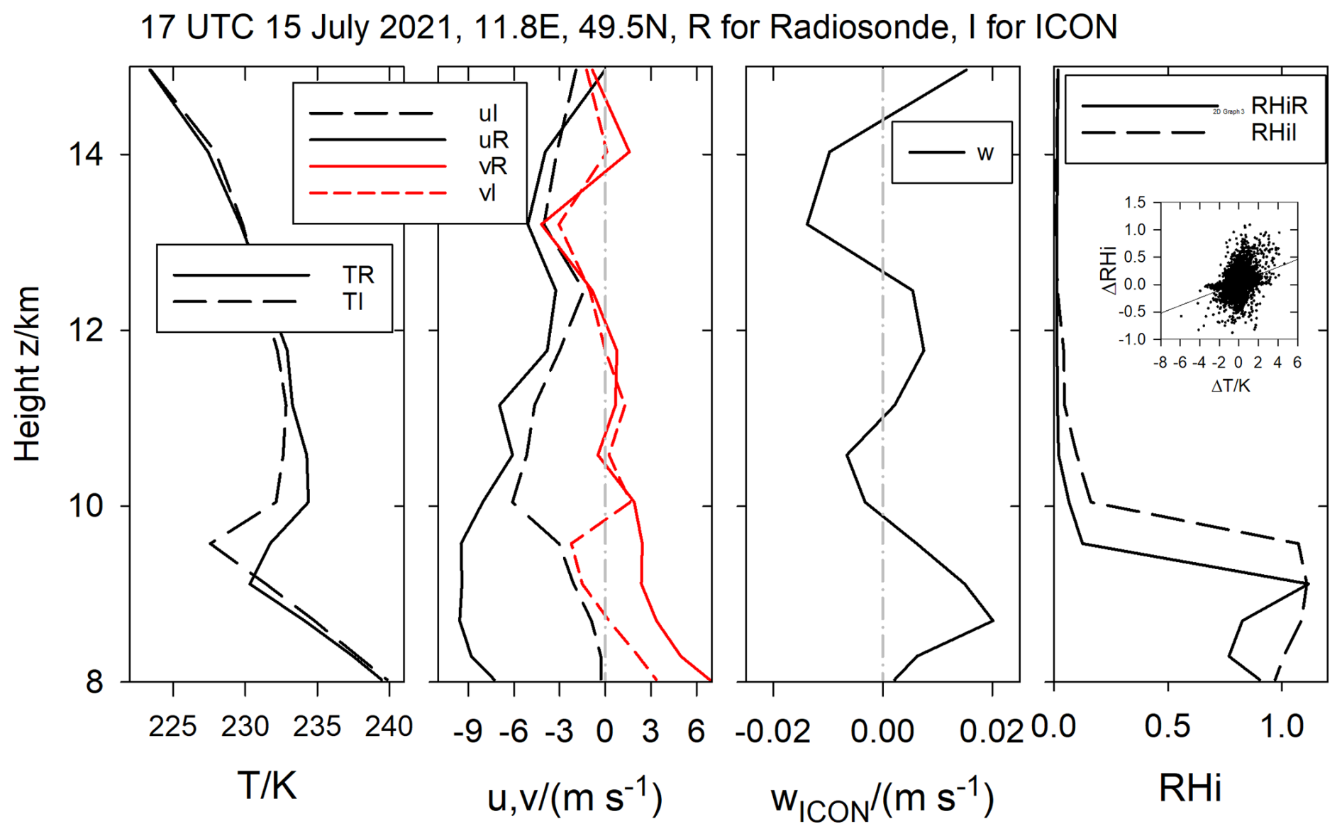
Figure 3 Example of an observed and modelled vertical profile with large RHi differences. From left to right: Temperature, horizontal wind components, modelled vertical wind, and relative humidity over ice, RHi. The “R” in legends refers to the radiosonde and the “I” to the ICON data. The largest difference ΔRHi between modelled and observed RHi values occurs near the tropopause at about 9 km altitude. The insert in the last panel shows that ΔRHi in such profiles is not always but often correlated with corresponding temperature differences ΔT.

The probability density functions (pdfs) of the simulated and observed RHi values, see Fig. 4a, agree within the rms differences of individual pdf values of the four 36 h-time periods studied. In areas where the atmosphere is cold enough to form short-lived contrails, the pdfs for both the observations and the model results start with a peak at low RHi and show a secondary peak at ice saturation. The 2-way coupling changes the RHi pdf only to minor degree: the differences are visible at high RHi, but only when the pdf is plotted in logarithmic scales. Hence, contrails reduce ambient RHi at high RHi values. The differences between the 2-way and 1-way coupling simulations are smaller than found in a global climate model study (Fig. 1 in Schumann et al., 2015). The pdfs in Fig. 4b, derived from ICON results agree with the observations clearly better than when using IFS results. The pdf results at radiosonde positions and along flight tracks, Fig. 4a and c, show consistent results with small differences, reflecting regional or sampling differences.

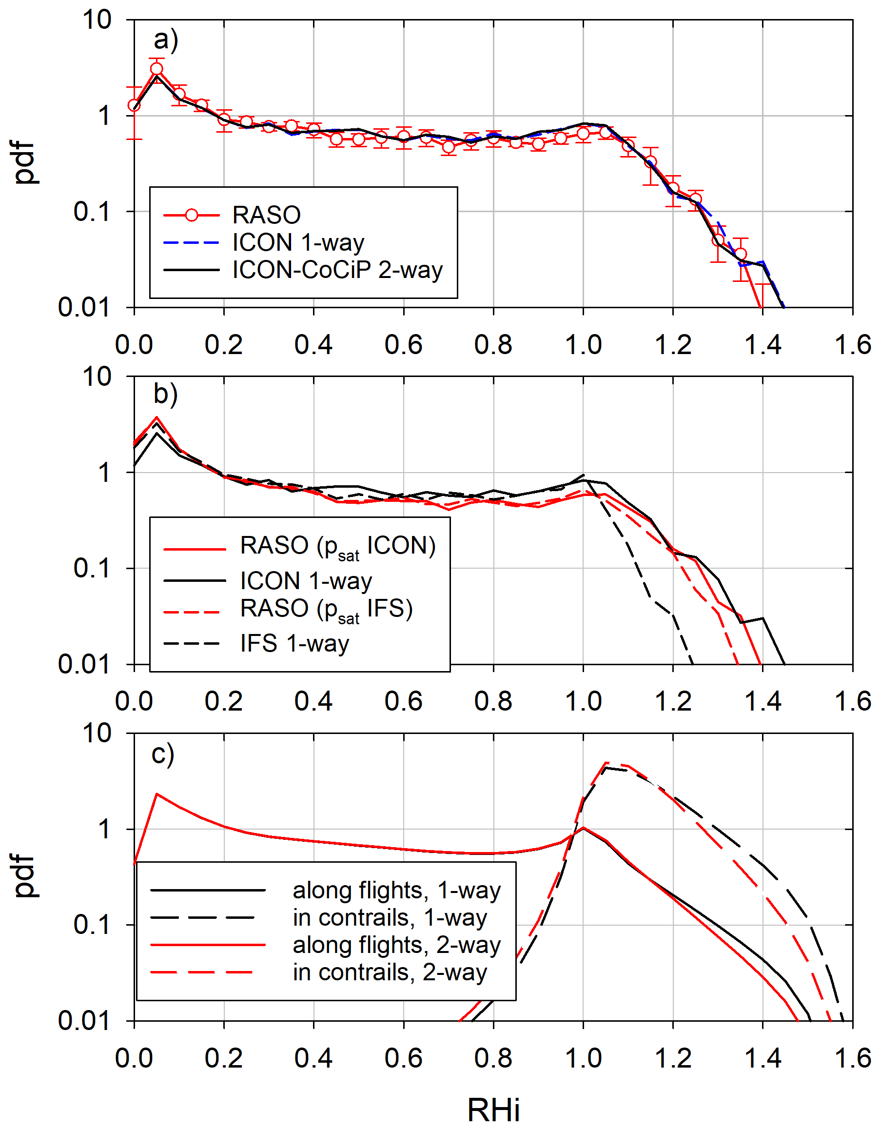
Figure 4 Probability density functions (pdf) of the occurrence of relative humidity with respect to ice saturation (RHi) in air cold enough for contrail formation on fine grid on average over four 48 h periods (starting 00:00 UTC 1 January, 25 June, 15 July, 15 December 2021). The curves show the mean values over the four runs for the different days. The error bars in panel (a) depict the rms values of these mean values. (a) The red curve with error bars shows the observation pdf from Vaisala RS 41 radiosondes in the Northern hemisphere (28–65° N, 166° W–145° E, over Europe, North Africa, Korea, Japan, Western Alaska, Southern Greenland, and Iceland). The other curves represent the ICON forecast results on fine grid without (1-way, dashed, blue colored) and with (2-way, full, black) contrail feedback. (b) Mean pdf from radiosondes (red) and models (black), comparing ICON and IFS forecast data. The radiosonde results differ because of different ice saturation pressure functions in ICON and IFS. (c) Pdf of RHi computed along GAIA traffic flight tracks (full curves) or inside CoCiP contrails (dashed) using ICON output without (1-way, black) and with coupling (2-way, red) with CoCiP.

Similar studies with the operational ICON version instead of the new one with improved ice microphysics showed that only the new version shows realistic ice supersaturation results (Hanst et al., 2025).

3.2 Contrail properties in comparison to observations

As a test to demonstrate that the contrail properties computed with CoCiP are reasonable, we compare model results with observations for young and aged contrails (ages of 1–20 000 s after contrail formation) for a wide set of in-situ and remote sensing measurements as collected in the Contrail Library (COLI) (Schumann et al., 2017), see Fig. 5. Note that we compare contrail properties for same ages but different ambient conditions. So, the model and observation results can only be compared statistically. Nevertheless, the figure shows reasonable agreement of the CoCiP-modelled contrail properties with available measurements. The results shown were obtained in the 2-way coupling mode. The differences to the 1-way mode (not plotted) appear minor in such plots with logarithmic scales.

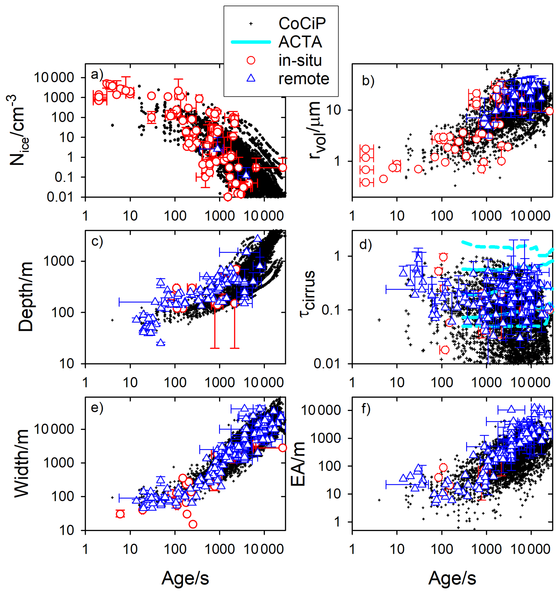
Figure 5 Comparison of simulated contrail properties from CoCiP with in situ, remote sensing, and satellite observations from the contrail library database, COLI (Schumann et al., 2017) versus contrail age. The contrail properties compared include the (a) contrail ice particle number concentration; (b) ice particle volume mean radius; (c) geometrical contrail depth; (d) solar optical depth; (e) geometrical width; and (f) total extinction, i.e. integral of the optical extinction over the contrail cross-sectional area, which influences the contrail radiative forcing. The red data points are from in-situ measurements, blue data points are from remote sensing, and the cyan lines in (d) represent the 0th, 10th, 50th, 90th, and 100th percentiles from METEOSAT satellite data using an automatic contrail tracking algorithm (ACTA) (Vázquez-Navarro et al., 2015). The black data points are the CoCiP-simulated contrail properties for a random subset of results for the first 2 d after 00:00 UTC 15 December 2021, with coarse grid.

Similar comparisons were presented before in Schumann et al. (2017), comparing observed contrail properties with model results from CoCiP coupled to a global climate model (Schumann et al., 2015), and in Teoh et al. (2024b) comparing with results of the CoCiP coupled 1-way to ECMWF-ERA5 reanalysis data. Compared to the global climate model study, the spread of data in the present simulation is smaller, which may be partly due to the shorter time period (few days) considered in the present study compared to the full year of simulation results in the earlier comparison. But we see a more consistent behavior, without tendency changes at larger ages. Compared to Teoh et al. (2024b), we note that our contrail depth and width values are consistent with the observations without humidity corrections and without limiting the depth of the contrails to selected maximum value, as in the earlier study. Although we are aware of discrepancies between plume properties in the early stage of contrail formation (Dischl et al., 2024; Harlass et al., 2024; Märkl et al., 2024), these difficulties do not appear to be crucial for the aged contrails. This does not exclude improvement potentials, e.g., with respect to the influence of nonvolatile particles in contrail ice formation for individual contrail cases (Ponsonby et al., 2025).

3.3 Contrail formation as a function of ambient humidity and cirrus

Here we check whether the ICON–CoCiP-simulated contrails occur mainly in clear ice-supersaturated air or inside optically thin or thick cirrus. For this purpose, the “thickness” of contrails is measured by the effective emissivity ${\text{EA}}^{\prime }=\text{EA}\exp (-\mathrm{0.2}{\mathit{\tau }}_{\text{cirrus}})$, EA is the area-mean extinction, as plotted in Fig. 5, i.e., the integral of the extinction β over the contrail cross-section A, equal to the product of solar optical thickness τ of the contrail times contrail width $W,\text{EA}=\mathit{\beta }\text{A}=\mathit{\tau }W$. The factor exp (−0.2τ_cirrus) is used to account for shielding of radiation by cirrus with solar optical depth τ_cirrus above the contrail. The factor 0.2 is a rough approximation to crystal habit dependent fit values δ_lc, δ_sc, and ${\mathit{\delta }}_{\text{sc}}^{\prime }$ for longwave and incoming and reflected shortwave shielding contributions, listed in Table 1 of Schumann et al. (2012). The ambient cirrus is characterized by two parameters: its ice water content, expressed as the equivalent relative humidity of the IWC, RHi(IWC), and its total solar optical thickness TACI, from TOA to mid troposphere (450 hPa).

Figure 6a shows that contrails form in CoCiP for a wide range of ambient humidity, both inside and outside thick cirrus. Figure 6b–d show that contrails with large thickness EA^′ form and persist mainly in ice supersaturated air masses (RHi>1) within thin ambient cirrus (small values of RHi(IWC) and TACI). These findings are qualitatively consistent with what one can observe (Jensen et al., 2001; Li et al., 2023).

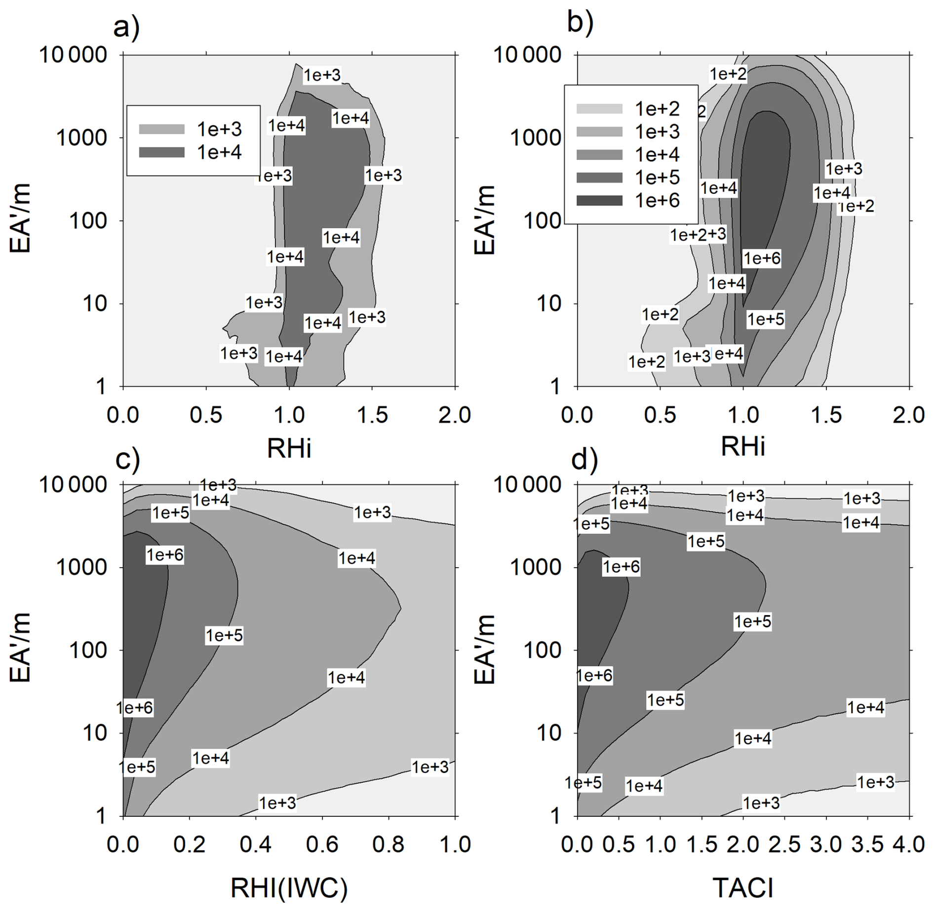
Figure 6 Occurrence number of contrails with optically effective cross-section area EA^′, with ${\text{EA}}^{\prime }=\mathit{\tau }W\exp (-\mathrm{0.2}{\mathit{\tau }}_{\text{cirrus}})$, counted in the sum over four 48-h-simulations starting in four days in 2021 as before. Here τ is the solar optical thickness of the contrail, W is the contrail width and τ_cirrus is the solar optical depth of cirrus above the contrail. The panels show the occurrence numbers (a) for freshly formed contrails versus relative humidity over ice (RHi) in the ambient air, and (b–d) for ageing contrails versus (b) ambient RHi, (c) ambient cirrus ice water content converted to relative humidity RHi(IWC), and (d) total solar optical thickness τ_cirrus of ambient cirrus (TACI) between TOA and 500 hPa.

3.4 Tests of the Radiation Transfer models

Other than in an earlier coupling of CoCiP with a global climate model (Schumann et al., 2015), the radiative effects of contrails are computed in the host model. In addition, the libRadtran-based CoCiP RF model (Schumann et al., 2012) is used here for comparisons. In both the coupled and uncoupled modes, ICON computes radiation transfer using the ecRad radiation solver of the ECMWF (Hogan and Bozzo, 2018). Initial tests with the ecRad's McICA scheme showed large spatial and temporal variability (“noise”) from grid point to grid point, overlapping the contrail effects. Part of the noise was caused by McICA using random numbers to represent realistic cloud heterogeneity and overlap. Replacing McICA in ecRad with the Tripleclouds scheme (Shonk and Hogan, 2008) requires more computing time to represent in-cloud heterogeneity but reduces noise.

The comparability of radiative forcing (RF) estimates from ecRad with CoCiP was tested following Myhre et al. (2009) (but without using “Myhre” particles, i.e., radiation scattering properties independent of particle size): For this test we compute the TOA and BOA RF values caused by a globally uniform cirrus layer of 300 m thickness, at 11 km top height, with 100 % cover, fixed effective radius of 10 µm, for a set of values of the optical depth τ_cirrus, in simulations for the four days as considered before, by taking the difference of the net downward radiative fluxes in a simulation with the cirrus disturbance minus that without the disturbance. After finding weak variability of the global mean results during full days, we compare the results for a set of parameters for the first hour after model start. For a few cases, we also compared RF values computed with Tripleclouds and McICA (not shown here) and found that these differ in the 5 %-range.

Figure 7a and b depict the RF results as a function of τ_cirrus as obtained with ICON-ecRad in the 2-way mode and with the libRadtran-based CoCiP model in the 1-way mode at TOA. Figure 7c shows corresponding ICON results at the surface (BOA). As indicated by the error bars, the variation of the RF magnitudes is small over the various days considered. The net RF is positive at TOA, but negative at BOA, as expected (Khvorostyanov and Sassen, 1998; Meerkötter et al., 1999; Hong et al., 2016). Further analysis of the data revealed that while RF at TOA is dominated by upward fluxes (since the solar input is unchanged and the downward LW flux is practically zero), the BOA-RF is dominated by the cirrus induced changes in downward fluxes, and hence weakly sensitive to surface properties (surface albedo and emissivity), except for large surface albedo.

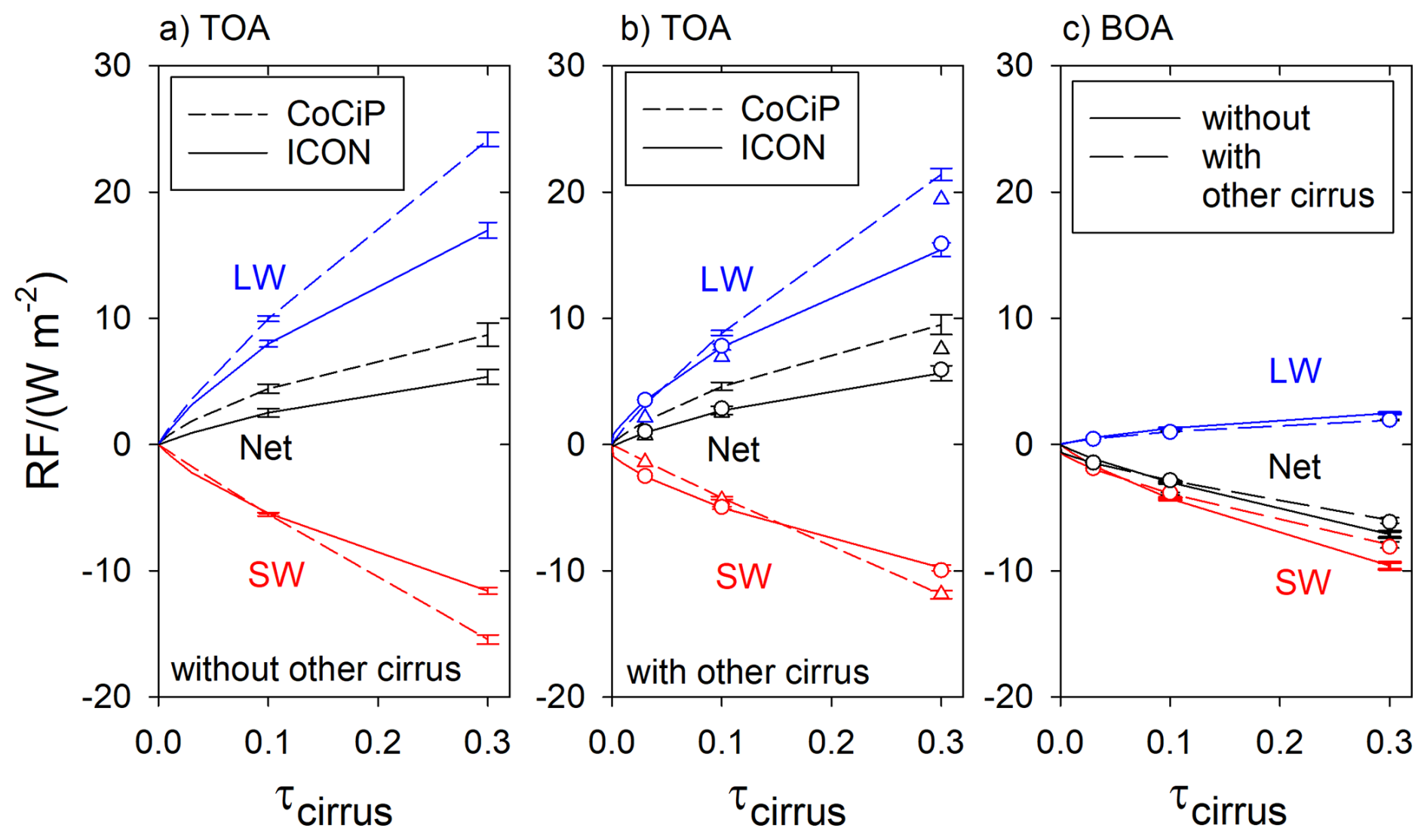
Figure 7 Results of a radiation model test for shortwave (SW), longwave (LW) and net (LW + SW) radiative forcing (RF) from a globally homogenous cirrus layer versus its solar optical depth (τ_cirrus) as obtained with ICON-ecRad (difference between coupled and non-coupled mode) and with the libRadtran based CoCiP (uncoupled 1-way mode) on coarse grid. The lines and error bars represent the mean values and rms deviations for 4 d. (a) Top of the Atmosphere (TOA) from CoCiP (dashed) and ICON (full lines), for case with background cirrus. (b) Same without background cirrus. Note that the curves start from nonzero RF for small τ_cirrus>0 in panel (a). (c) Bottom of the Atmosphere (BOA) as derived from ICON-ecRad with (dashed) and without (full lines) background cirrus.

For optical depth τ_cirrus less than about 0.1, which is quite typical for domains with large contrail cirrus cover, both methods compute similar RF, but ICON-ecRad tends to compute higher RF magnitudes for very thin cirrus and smaller values for thicker cirrus. As a consequence, for widespread optically thin added cirrus or contrails, we have to expect larger global mean RF values from ICON than from CoCiP.

The RF fluxes are zero for τ_cirrus= 0, as expected, but the ecRad-results show a small stepwise change to nonzero values for small τ_cirrus, see Fig. 7a and c. This irritating behavior was found to be due to some radiative interaction of the added cirrus with the preexisting “background” cirrus. It disappears when the background clouds are excluded from the radiation transfer analysis in ICON-ecRad, see Fig. 7b and the full curves in Fig. 7c. Without background cirrus, the RF values start, as expected, linearly from zero for small values of τ_cirrus. A method that avoids this behavior has still to be found.

EcRad uses ice particle scattering properties from Fu (1996) and Fu et al. (1998) or from Yi et al. (2013), among others. We tested these two versions and found only small differences (order 5 %) for our application. Here, we use the Fu version because it imposes no lower limit for the ice particle effective radius. The alternative of Yi et al. (2013) applies to ice particles with radius>5 µm.

The stronger nonlinearity of the ecRad results triggered a revision of the CoCiP RF model as explained in Sect. 2.2., Fig. 8 shows the results of two CoCiP RF model versions for the cirrus test (with ambient cirrus) as just described. The new CoCiP RF model version captures part of the nonlinearity found in the ecRad results. This can be seen in Fig. 8, which compares the dependencies of RF on the optical thickness of the added cirrus layer. We see that the new version 2 of the libRadtran fit provides slighty larger RF values for small optical thickness of the added cirrus layer, more consistent with the ecRad results. For optical thickness larger than about 1, the new model computes slightly smaller RF values.

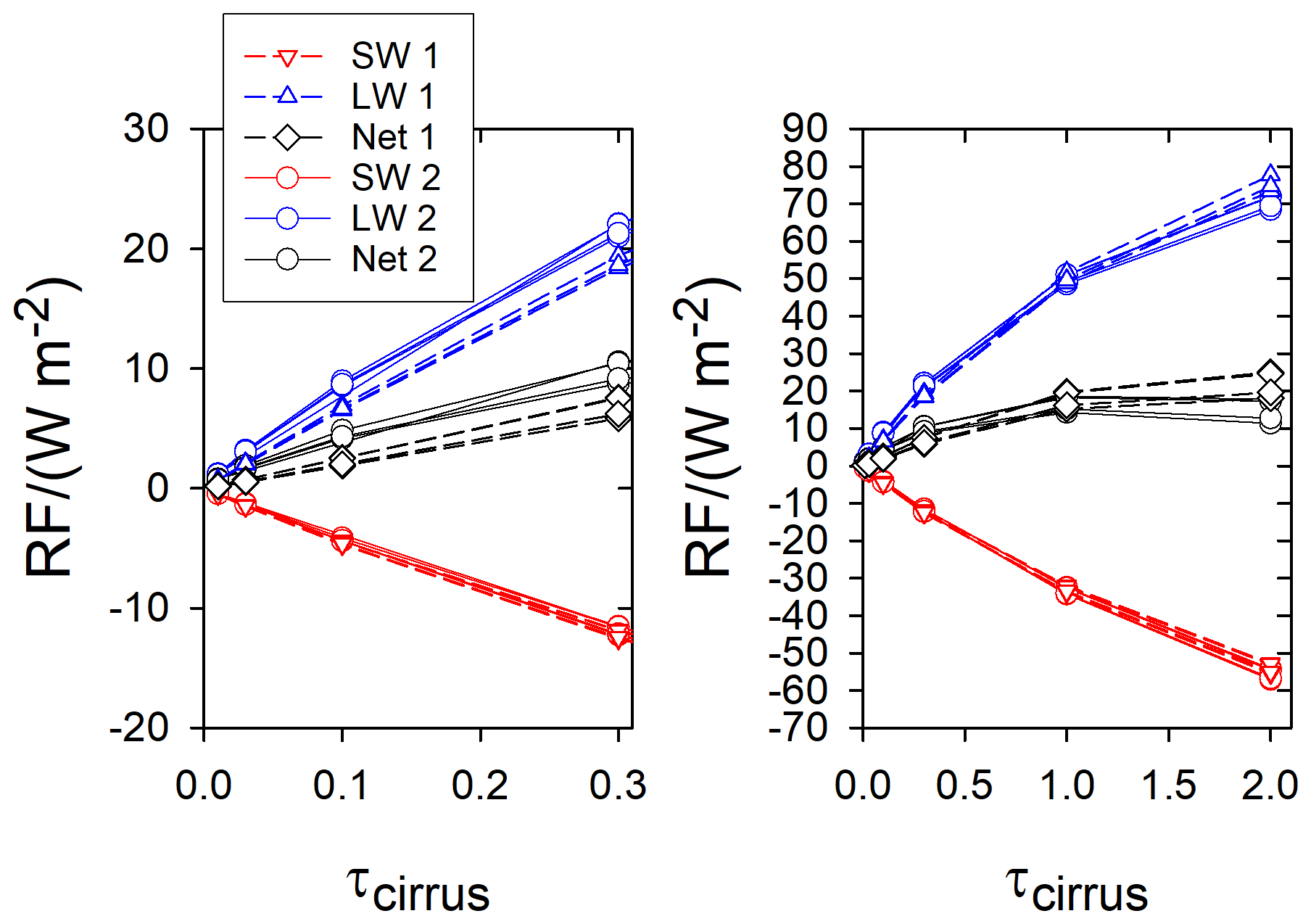
Figure 8 CoCiP-libRadtran results for SW, LW and net RF in the 1-way mode coupled to ICON as a function of the solar optical thickness τ_cirrus of an added uniform global cirrus layer for the four days considered (largest net RF in July) from model version 1 (dashed) and version 2 (full lines). Left for τ_cirrus≤0.3, right for τ_cirrus≤2.

Further comparisons (details not shown here) were performed of ICON and IFS TOA OLR and RSR fluxes with satellite data (METEOSAT (Vázquez-Navarro et al., 2013; Strandgren et al., 2017) and CERES Syn1deg Ed4 A (Wielicki et al., 1996)) at 1° horizontal resolution over “Europe”, (20° W–20° N, 35–60° N) for the four days in 2021 as before. Here, ICON underestimates the OLR by about 6 W m⁻² in the 1-way and 5.5 W m⁻² in the 2-way mode. Correlations between model and observation data start high (0.98) but decrease to below 0.8 within 48-h forecast time. Here, the IFS predictions show higher correlations (order 0.9 after 48 h). This indicates still existing cloud modelling issues in ICON, but not necessarily related to cirrus clouds.

4 Coupling Results

4.1 Spatial distribution

For orientation, Fig. 9 (left part) shows the global distribution of air traffic for one day, here measured in terms of day-mean area-specific fuel consumption above flight level (FL) 180 (about 5.5 km pressure height) with mean and maximum values of 1.4 and 240 kg (km² d)⁻¹. In the logarithmic color scales used, we see all routes including rarely used routes in remote areas; in linear scales, we would see mainly the high traffic density flight tracks over USA, Europe and the Far East.

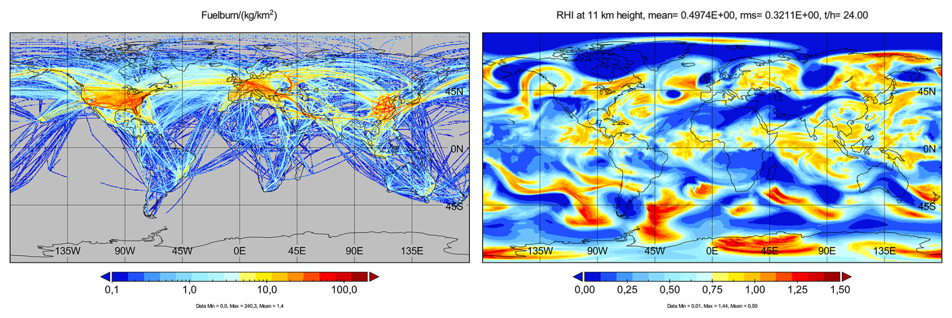
Figure 9 Left: Aviation fuel burn above 5.5 km height within 48 h since 00:00 UTC 25 June 2021, in kg km⁻². The data shown are based on GAIA (Teoh et al., 2024a). Right: The 24 h mean RHi field at 11 km above mean sea level for this day.

Note that the traffic in the first part of the year 2021 was still affected by the COVID crises. The total fuel burn values reached 0.448, 0.629, 0.680, and 0.682 Tg in the 48 h time periods after 00:00 UTC 1 January, 25 June, 15 July, and 15 December 2021, respectively, showing still reduced traffic at the beginning of the year 2021 and a recovery of traffic from COVID near the end of the year. Figure 9 (right) shows the day-mean distribution of relative humidity over ice for 25 June 2021. We see that the regions with ice supersaturation (RHi>1) where contrails are expected to be formed for nonzero traffic, are relatively large and often sharply bounded (in spite of smoothing in the plot by averaging over the day) by air masses with much lower RHi values.

Figure 10 shows the CoCiP-computed day-mean global contrail coverage induced by this traffic after 2 d, here in terms of solar optical thickness, first in the 1-way and then in the 2-way coupling mode, in logarithmic scales, and then the difference of these results in two different color scales. Comparing to the previous figure, we see that the contrails form mainly in domains with high traffic density and high RHi (e.g., the eastern part of USA and southern part of Europe this day), as to be expected. The top two panels indicate that the general contrail features are nearly the same at this time regardless of the coupling modes. The plots show ICON-grid-cell averaged values of the optical depth of contrails with rather high (1.5) maximum values in areas with high traffic density and high ice supersaturation. The global mean and maximum values in the 2-way mode (0.00166 and 1.20) are only a little smaller than in the 1-way coupling (0.00173 and 1.75). The lower panels show the optical depth difference of the two results in two different linear color scales, left changing from blue to yellow at the zero value and right without color change at the zero value. In the blue colored domains, the optical thickness is slightly smaller, as expected because the 2-way atmosphere feedback reduces the ambient humidity. But, In the red colored domains, the optical thickness is locally much larger (e.g. over Eastern USA) indicating unexpected nonlinear coupling effects, discussed further below.

The top left panel in Fig. 11 shows the TOA radiative forcing computed with CoCiP in 1-way mode from ICON fields. The left middle and lower panels in Fig. 11 show the TOA and BOA RF computed with ICON-ecRad with contrail feedback (2-way). As to be expected, we see strong net RF values both in areas with high traffic density, but surprisingly also large values with high spatial variability in areas far away from the regions with high traffic density. The maximum day-mean local ICON RF values (60 W m⁻²) are nearly double the maximum CoCiP values (34 W m⁻²). The 2-way ICON-ecRad result shows some correlation to the CoCiP 1-way result but the variability is surprisingly high. The plots are based on mean values over all time steps during that day. Without this dense time-averaging the variability would appear far stronger. This indicates that the variability is dominated by high-frequency noise. The noise would also appear far stronger in the plots if the discrete color scales would change color at the zero value. We find weaker noise in the LW RF fields (not plotted). Hence, most of the noise in the RF results is due to small, near-random displacements of clouds with fractional cloud cover, changing reflected solar radiation. Further analysis of the results shows that the displacements occur both horizontally and vertically. The variability is minimal at high latitudes with more stably stratified atmosphere and largest in regions with deep convection and strong precipitation, indicating pronounced nonlinearities in atmospheric dynamics, particularly related to vertical velocity and precipitation processes.

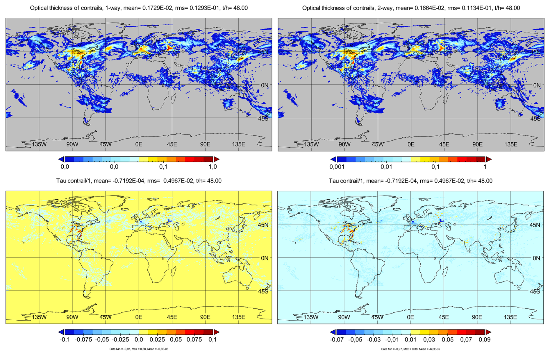
Figure 10 Solar optical depth of contrails on average over hours 24–48 after initiation at 00:00 UTC 25 June 2021. Top left panel: 1-way mode, top right: 2-way mode, bottom: difference. The top panels are color coded in logarithmic scales; the bottom in linear scales, with two different color scaling: the left emphasizes small variations near zero, the right shows optical depth variations exceeding ±0.01. The plots in Figs. 10–13 are coarse grid simulation results.

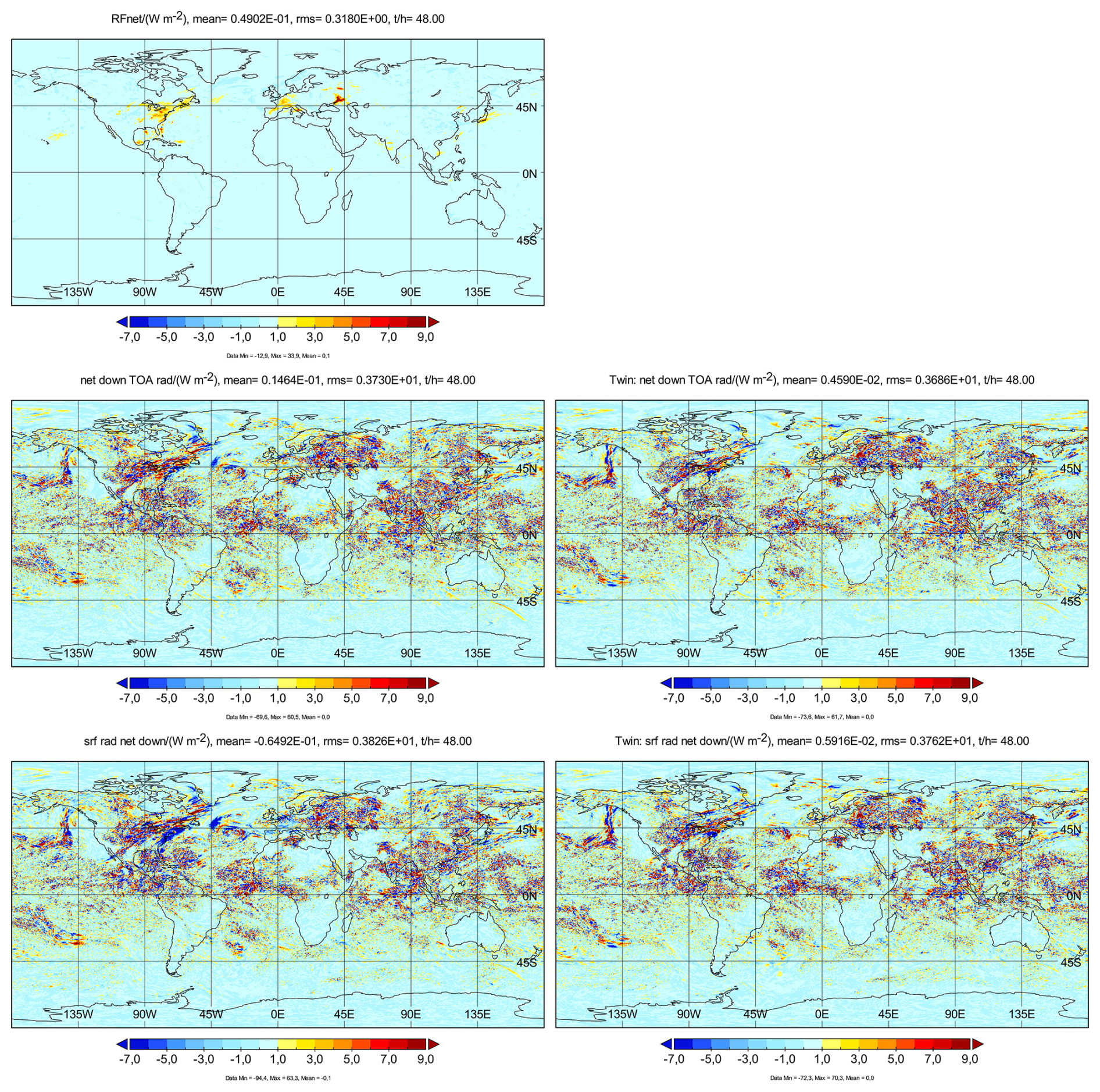
Figure 11 Radiative forcing in W m⁻², on average over day 2 after initiation at 00:00 UTC 25 June 2021 (coarse grid). Top: CoCiP RF model. Middle row: net downward radiation difference between 2-way and 1-way mode computed with ecRad in ICON, at TOA. Bottom row: same as middle for BOA (surface). The left panels show the effects of contrails. The right panels show the RF results from the twin experiment with random instead of contrail forcing. Note that the color scales selected do not include the extreme values of order 80 W m⁻² and are insensitive to noise within $\pm \mathrm{1}\mathrm{W}{\mathrm{m}}^{-\mathrm{2}}$.

As announced before (Chapter 2), we compare to twin experiments and present the differences between simulations with and without random disturbances in the initial conditions, without air traffic and contrails. The right panels in Fig. 11 show the RF response of the ICON results in the twin experiment with random disturbance of magnitude 10⁻¹². The random part of the pattern on the right is surprisingly similar to the left columns. Still, the contrail impact in domains with high traffic density is stronger and the mean and rms values of the run with contrails are larger than the corresponding values from the twin-experiment. So, the ICON–CoCiP RF results in the coupled mode appear significantly different from the twin experiment. Additional simulations (not shown here) with a factor 100 higher random disturbance of the initial values (10⁻¹⁰) show similar random patterns but of about the same magnitude. So, the response to the disturbances in highly nonlinear.

A similar figure (not shown here) with corresponding results for day 10 after initialization reveals RF values with far larger variability, now also with some smooth pattern changes, in particular in the Northern hemisphere, where most traffic occurs, but with still small mean values. Hence, the weather in the 2-way mode has changed strongly compared to the 1-way mode after 10 d, causing large RF variability, not only locally, as discussed further below.

Any surface temperature change induced by aviation would be of high relevance with respect to its climate impact. Figure 12 shows that contrails indeed change the surface temperature locally by up to 2 K even in the 24 h mean but hardly in a systematic and statistically significant manner. The lower panel in this figure shows that contrails also impact precipitation. The results are very spotty, again with surprisingly large extreme values reaching up to about $\pm \mathrm{30}\mathrm{mm}{\mathrm{d}}^{-\mathrm{1}}$ for precipitation in the day-mean locally. The global day-mean change values are very small, below ±0.8 mK in temperature and $\pm \mathrm{0.8}\mathrm{\mu }\mathrm{m}{\mathrm{d}}^{-\mathrm{1}}$ in precipitation. Again, the contrail-induced temperature and precipitation changes are not much different from the random disturbances in the twin experiment.

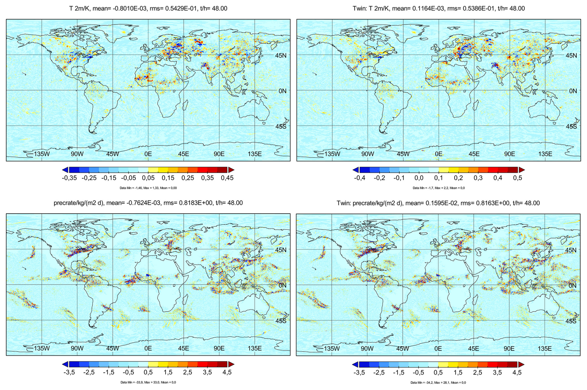
Figure 12 Near-surface (at 2 m height) temperature change (top panels) and precipitation rate change (bottom) on average over day 2 of the simulations starting 25 June 2021 (coarse grid). Left with contrails, right with random disturbances (twin experiment).

Closer inspection of the plots in higher spatial resolution, see Fig. 13, shows that the large extreme values in temperature and precipitation changes are mainly caused by small spatial shifts of air masses with strong spatial gradients. The largest temperature changes occur in domains with strong precipitation, as on this day over continental USA and Eastern Europe, and in correlation with large precipitation position changes. However, notably, random noise in the initial values causes similar changes. Hence, the contrail effects on atmospheric dynamics cannot be easily distinguished from those caused by random disturbances.

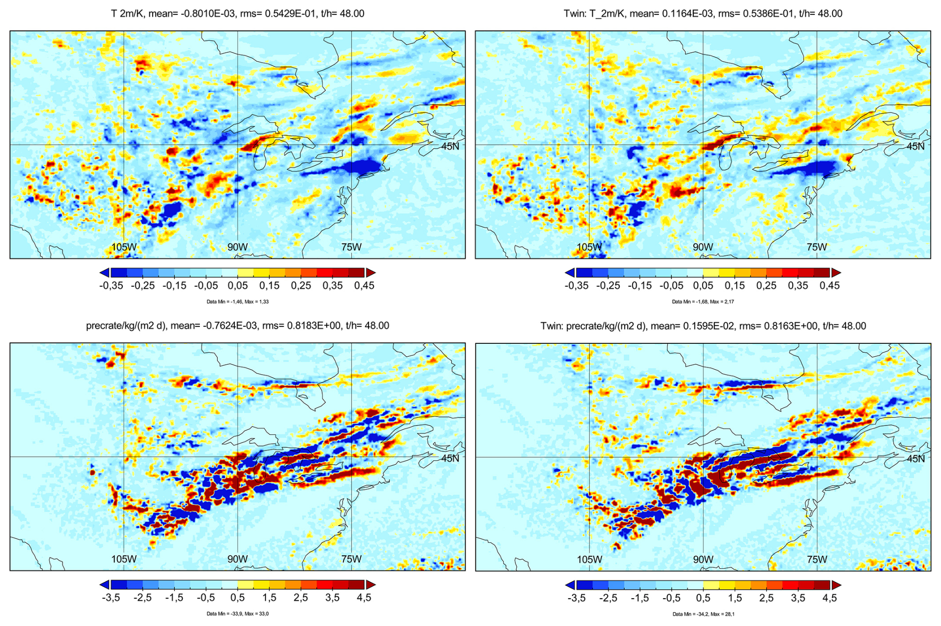
Figure 13 Left panels: Regional extract (over North America) from previous figure, showing that the changes of the 2 m-temperature (top panel) and precipitation changes (bottom) occur mainly by lateral shift of rain bands. Right panels: Same for the twin experiment, showing similarly shifted bands.

The results so far have shown several changes in the contrail effects due to the 2-way coupling and partly surprising similarity between contrail and twin experiments. In the next section, these effects will be further discussed with respect to the mean values and then summarized in Sect. 5.

4.2 Mean values

Next, we present global and regional mean values. Figure 14 shows the global mean SW, LW and net RF values as a function of the forecast time at TOA and BOA as analyzed with CoCiP in the 1-way mode and as computed from the difference of ICON results with (2-way) and without (1-way) contrail feedback. Each RF value plotted for a given time measures the integral global downward flux of radiation energy over the past 24 h time interval at TOA or BOA, divided by the Earth surface and the time interval, in W m⁻². So, the first value is the mean RF from time 0–24 h.

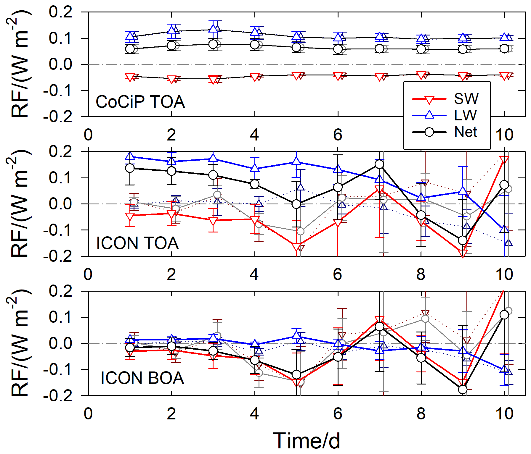
Figure 14 Daily mean RF values (in W m⁻²), showing the contrail induced SW RF in red (triangles down), the LW RF in blue (triangles up), and the net value in black (circles) on average over the four test days in 2021 versus forecast time. The errors bars indicate the rms values from the 4 simulations. The dotted curves are the results of the twin experiment. They are plotted with temporally slightly shifted error bars. The top panel shows the RF as computed with CoCiP for given atmosphere and contrail properties. The second panel shows the RF as derived from the differences between the downward TOA fluxes in the ICON runs with and without contrail feedback. The bottom panel shows the same for the surface fluxes. Note the correlation between ICON TOA and ICON BOA RF values for later days.

At TOA, we expect a SW cooling, LW warming, and net warming. This is confirmed with the CoCiP RF model, see the top panel in Fig. 14. As explained before, the contrail RF is computed with CoCiP for these two ICON simulations but without contrail feedback on ICON. Here any random disturbance in the ICON initial values has negligible impact. The mid panel shows the differences between the two ICON runs with and without contrail feedback, and we see the same tendency as in the CoCiP results, but large differences in the details. The ICON–SW effect is not strictly negative and the ICON–LW and Net RF values are nearly double the CoCiP values. Obviously, random disturbance in the ICON initial values have strong impact on RF. With the coupled ICON–CoCiP model we also can compute the RF at the bottom of the atmosphere (BOA), see bottom panel of Fig. 14. As to be expected, the RF magnitude is smaller at BOA than at TOA and tends to be slightly negative, though with scatter far larger than the mean. We see a correlation between the oscillations in the TOA and BOA RF values. This indicates that the weather changes after some days not only at small but also at large scales. The plot shows also the RF results from the twin experiment (difference of the radiative fluxes in the simulations with and without random disturbance). The twin RF results start small but grow quickly and the oscillations correlate also with the contrail RF oscillations at late times. Factor 100 changes in the random amplitudes of the initial disturbances cause only small changes (not plotted) in these oscillations. This indicates again that the weather changes are more strongly controlled by the ambient weather state than by the amplitude of the disturbances. We clearly see that the RF values due to contrails in the 2-way mode can no longer be distinguished from the twin experiments after a few days, which will be discussed further below.

The contrail lifetime of all contrails in 1-way mode after 48 h forecast time on average over the 4 simulated days is 1.75±0.22 h (largest in winter). The total energy forcing (EF) from all flights computed with the CoCiP-RF model in the 1-way mode amounts to 2.5±1 in unit of 10¹⁸ J d⁻¹. In the 2-way mode, with reduced ambient humidity, the age is only 2 % longer because of reduced ice particle sedimentation, but the EF is 28 % smaller because of optically and geometrically thinner contrails. The age is shorter than the 2.25 h found in the study of Teoh et al. (2024b). The CoCiP-derived EF depends strongly on the actual traffic and weather but the magnitude is similar to the annual mean value of $\mathrm{1.4}\times {\mathrm{10}}^{\mathrm{18}}\mathrm{J}{\mathrm{d}}^{-\mathrm{1}}$ reported by Teoh et al. (2024b) for the year 2021. The EF from contrails using the ICON-ecRad radiation fluxes in the difference between 2-way and 1-way mode has not been analyzed so far, because that requires that the ICON results from the run without contrail feedback is available at the time when the coupled model simulates the contrails with feedbacks. However, such coupling is feasible and could be done in the future.

Figure 15 shows mean temperature profiles versus height for subsequent days after forecast start on average over the four starting days considered. The black curve shows the daily mean values of the run in the 1-way mode, with very small variability from day to day. The minimum temperature at 17 km height indicates the global mean height of the tropopause. The colored curves reveal the mean temperature changes due to contrail feedback on average over the four runs. Here we show the results only for the first 5 d of the 10 d forecasts. The results for later forecast days are not shown because of increasing variability. For the first 5 d, we see that the contrails induce a mean warming in the upper troposphere at heights between about 6 and 13 km. For the first 5 d, the contrail induced temperature increases are higher than the changes seen in the twin-experiments, so we see a significant contrail-induced warming.

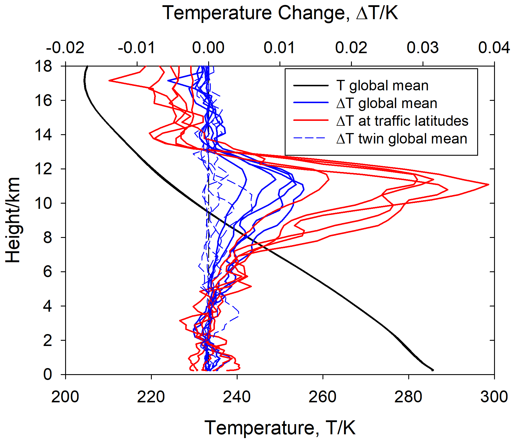
Figure 15 Daily and global mean profiles of temperature versus geopotential height for 5 subsequent days on average over four simulations for different starting dates (as before). The mean values are also averages over the last 24 h of the forecasts. The black curves show the mean temperature of the run in the 1-way mode. The profile variance from the 5 forecast days is within the thickness of the curve plotted. The colored curves refer to the upper temperature-difference scale. The blue curves depict the mean temperature differences between the runs with contrail feedback relative to the runs without feedback for five subsequent forecast days. The red curves show the same, but here the global mean values are weighted with the annual mean air traffic fuel consumption density as a function of latitude. The thinner blue dashed curve shows the global mean temperature difference profiles for the twin experiment.

The red curves show globally averaged results weighted with the latitude-dependent annual mean traffic density. As to be expected, the warming effect is not globally uniform but largest in areas with large traffic density. Also, we see a cooling tendency above the contrails because less longwave radiation reaches the stratospheric ozone. Notably, the temperature changes below about 5 km are close to zero. In the future, it might be worthwhile to compute also mean vertical and horizontal turbulent fluxes of sensible and latent heat to see how advection and turbulence add to radiation fluxes and to compare with previous studies (Schumann and Mayer, 2017).

The global mean temperature changes shown in Fig. 16 at the contrail level (about 11 km height), and at the surface show more or less uniform trends in the first 3–5 d, but then show larger values and strong variability from day to day, indicating chaotic weather responses, as obvious from the twin-experiment results. Again, as stated before, the chaos in the twin-experiments grows only slightly quicker (slower) when starting with factor 100 larger (smaller) initial random disturbances ε, but does not exceed the contrail-induced variability. The lowest panel in Fig. 16 depicts the forecast mean precipitation rates showing only insignificant changes. Hence, the global mean feedback of contrails on the hydrological cycle is weak over the first forecast days.

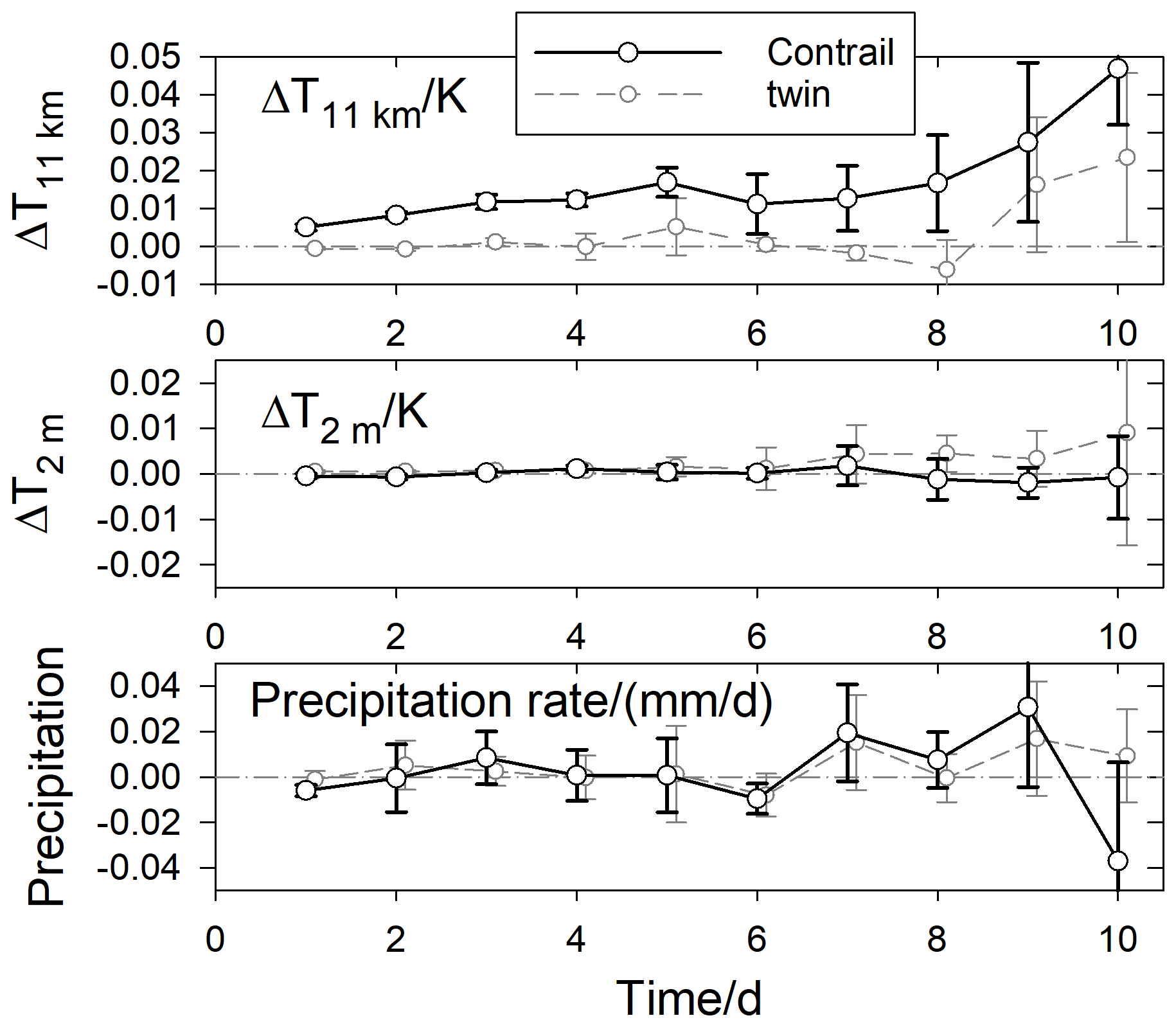
Figure 16 Changes of global mean temperature (at 11 km and 2 m heights) and precipitation rate versus forecast time on average. Each value denotes the mean over the last 24 h. The error bars denote the rms of the simulation results for 4 different forecast days. Thick curves: with contrails; dashed curves with smaller and temporally slightly shifted grey symbols: results from the twin experiment.

4.3 Variability analysis

As we have seen in the preceding sections, contrails induce local disturbances at the resolution limit of the host model growing in amplitude and in spatial scales with forecast time. Detailed inspection of the data reveals that the contrails change the local circulation and induce temperature and velocity changes like gravity waves spreading sideward and vertically, as expected (Jensen et al., 1998a). Besides using gravity wave schemes for orographic and non-orographic gravity waves, ICON, being a non-hydrostatic model, resolves gravity waves at least partly. Small horizontal position changes of ambient clouds induce large local changes in the vertical radiation fluxes. Several contrails forming at close distances in an ice-supersaturated air domain cause overlapping disturbances. These disturbances obscure any systematic change due to single contrails. In addition, the contrail disturbances may overlap with numerical disturbances near the resolution limit.

Following studies of weather predictability (Zhang et al., 2003; Selz et al., 2019), we measure the time evolution of the difference between the 1-way and 2-way simulations by analyzing mean variances and the mean spectrum of kinetic energy $\text{KE}=\mathrm{1}/\mathrm{2}(u^{\mathrm{2}}+v^{\mathrm{2}})$ of the horizontal windfield versus wavelength 2πk⁻¹ with wavenumber k in the 1-way mode, and the kinetic energy spectrum of the horizontal velocity differences $\text{DKE}=\mathrm{1}/\mathrm{2}\left(\right(\mathrm{\Delta }u{)}^{\mathrm{2}}+\left(\mathrm{\Delta }v{)}^{\mathrm{2}}\right)$ between the 2-way and 1-way simulation results. In addition, we show mean values and spectra $\text{KEw}=\mathrm{1}/\mathrm{2}{w}^{\mathrm{2}}$ of vertical velocity and $\text{DKEw}=\mathrm{1}/\mathrm{2}(\mathrm{\Delta }w{)}^{\mathrm{2}}$ of vertical velocity differences. One-dimensional zonal Fourier spectra are computed at a fixed altitude of 11 km corresponding to the mean flight level for ten-day forecast with the coarse grid (panel a in Fig. 17) and for three-day forecast with the fine grid (panel b). As in Selz et al. (2019), the spectra are computed from Fourier transforms of spatially interpolated discrete velocity values, with 1440 grid points along several parallel latitudes, and averaged from 30–60° N. The spectra shown are the kinetic energy spectra multiplied with the wave number k. Hence, the energy spectra have the units of velocity squared. Because of this multiplication, the spectral slope is −2 at large scales and not −3 as we would expect without this factor for nearly two-dimensional large-scale geostrophic motions (Nastrom and Gage, 1985). In addition, we see a weak increase of KEw with wavelength near to the power $\mathrm{1}/\mathrm{3}$ at scales between planetary scales (>5000 km) and mesoscales (<500 km), before the KEw spectrum decreases at shorter wavelengths. A power $\mathrm{1}/\mathrm{3}$-increase of KEw is consistent with a quadratic decrease of the KE spectrum (Skamarock et al., 2014; Schumann, 2019). The results do not show spectral ranges from the inertial range, here with power $-\mathrm{2}/\mathrm{3}$ for KE and KEw, and no damping at smaller wavelengths as found in other studies (Craig and Selz, 2018). Instead, we see increases in the spectra at short wavelengths, presumably from the small-scale convective activity in summer at Northern midlatitudes. From the results for 3d on the fine grid (Fig. 17b), we see basically the same trends and same magnitudes at large scales, but more reasonable mesoscale spectra with flatter downscaling between wavelengths of 50 and 200 km. So, the dip seen in the mesoscale spectra on the coarse grid are partly caused by numerical approximations.

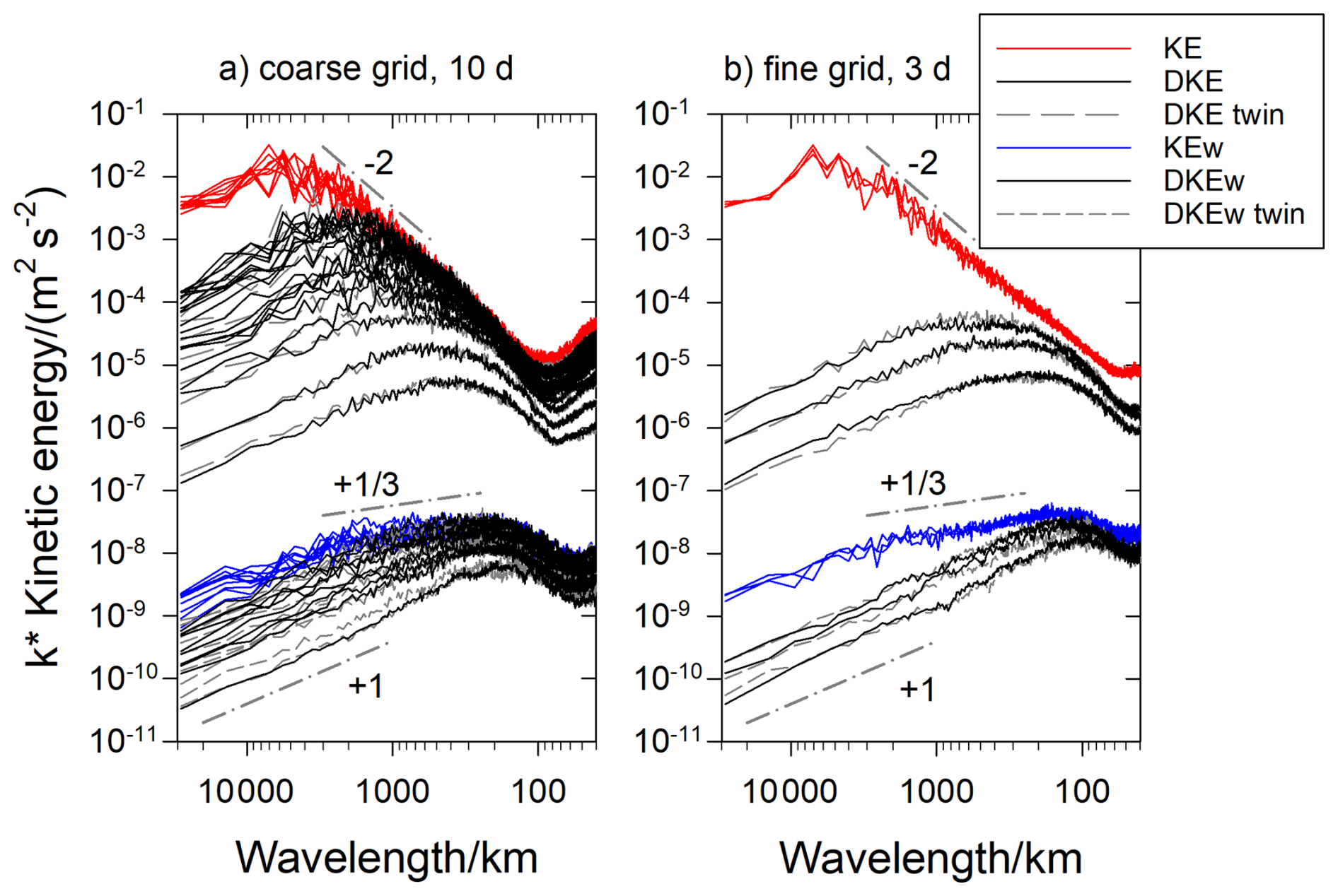
Figure 17 Spectra of kinetic energy multiplied with wavenumber k, $k=\mathrm{2}\mathit{\pi }/\text{wavelength}$, of horizontal velocities (KE) and of vertical velocity (KEw) from ICON and corresponding spectra (DKE and DKEw) of the velocity differences between the ICON–CoCiP 1-way and 2-way runs, (a) for 10 d forecasts on the coarse grid, (b) for 3 d forecast on the fine grid, both starting 00:00 UTC 25 June 2021. The curves show 24 h mean values at subsequent days. For KE and KEw, the curves fluctuate irregularly from day to day. For DKE and DKEw, the values grow with time from day to day. Straight dash-dotted lines indicate the −2 and +1 and $\mathrm{1}/\mathrm{3}$ power-law slopes. The grey dashed lines shown for DKE and DKEw spectra show the results of the twin experiment. The twin results for KE and KEw are not plotted, since they are virtually undistinguishable from the (red and blue colored) contrail results.

The kinetic energy of the velocity differences (DKE and DKEw) starts from zero at time of initialization, but then grows quickly with time. We see that the difference spectra remain below the background KE and KEw spectra over the ten-days forecast period but reach the background spectra, first at shorth wavelengths after a few days, and first for vertical velocity and later for horizontal velocities.

When comparing the spectra of DKE and DKEw due to contrails with those due to random disturbances (the grey curves in Fig. 17), we see strong similarity. Hence, the nonlinearity of the atmospheric dynamics causes an increase of the mesoscale deviations, in particular in vertical motions, induced by any small-scale disturbances, either due to contrails or due to random disturbances (as in the twin experiment) in the initial conditions up to dynamic saturation (Rotunno and Snyder, 2008).

Figure 18 shows that the mean background variances KE and KEw vary only a little over the forecast period, as expected for steady equilibrium conditions. The variances of the differences grow with time quickly during the first day and then grow exponentially (linear in logarithmic scales) for some days thereafter, indicating complete loss of predictability when reaching the level of the background variances. This chaos state is about reached for vertical velocity but not yet reached for horizontal velocity after ten days. From the near-linear increase of the logarithmic difference variances, one may guess that predictability is totally lost after an order 15–20 d, as expected (Rotunno and Snyder, 2008). As a special observation, we note that the summer cases (in June and July) approach full chaos more quickly (in spite of smaller horizontal kinetic energy) than the two winter cases (in January and December), likely because of stronger convective activity over the Northern continents, with weaker mean winds, enhancing nonlinear scale interactions in summer. The importance of convection for perturbation growth in butterfly experiments has been noted before (Selz et al., 2019). Hence, the growth rate of small-scale disturbances depends on the state of the atmosphere. We also prepared such plots from the twin experiments with initial disturbances varying from ${\mathrm{10}}^{-\mathrm{14}}-{\mathrm{10}}^{-\mathrm{10}}$. We found that the results look very similar to the contrail results, and are virtually independent of the initial amplitude of the random disturbances applied.

5 Discussion and Conclusions

5.1 Model tests

The tests presented show that ICON and CoCiP function reasonably, individually and in the coupled mode, though further improvements are desirable. ICON provides high quality weather data for contrail studies, in particular with respect to ice supersaturation (Fig. 2). In this respect, the new ICON version (“ICON-3”) performs clearly better than the operational version (“ICON-1”) as also shown by Hanst et al. (2025). CoCiP simulates contrails generally consistent with observations (Fig. 5). The comparison to radiosonde observations shows that the ICON two-moment ice microphysics model covers the whole range of ice supersaturation, with largest RHi values in cold air masses near the tropopause. Still, the agreement between the modelled RHi values and the measurements is not perfect. The model and measurement RHi values show similar mean values, but the rms differences reach 15 % and maximum deviations exceed 100 % locally. For temperature and horizontal windspeed the local deviations are far smaller. The local RHi deviations are weakly sensitive to the microphysics model parameters. They also depend on the forecast initial values and grid resolution used. We have to keep in mind that we compare grid cell mean values with 300 m vertical, 13 (26) km horizontal and 120 (240) s temporal grid spacing in the fine (coarse) grid with vertical mean values from the 1 s radiosonde data averaged over 20 hPa (about 600 m) intervals. The weak simulated vertical wind and its impact on nucleation could cause part of the RHi simulation errors (Kärcher and Lohmann, 2002). But this is not obvious and hard to overcome because the grid-scale vertical wind is strongly smoothed compared to local reality as long as the grid does not resolve sub-kilometer motion scales (Schumann, 2019; Dörnbrack et al., 2022).

The scores (Table 2) are significantly higher when restricting the comparison to cases with sufficiently cold ambient air in which the SAC is satisfied. It would be interesting to test whether the low ETS scores (0.09–0.25) reported by Gierens et al. (2020) comparing pressure-level ECMWF ERA5 reanalysis data with airborne MOZAIC humidity measurements are caused by large fractions of data from domains too warm for contrail formation. Though being aware of the limited coverage of the of data samples and limited conclusiveness of any scores (Hogan et al., 2010), we tentatively conclude from the results that the ICON model in fine resolution and with triangular interpolation gives slightly better scores than with coarse resolution and nearest neighbor interpolation, but the improvements hardly justify the additional computational effort. Notably, the predictions of ICON–CoCiP in the 2-way mode is mostly slightly better than in the 1-way mode (see Table 1, coarse grid). And, the ICON model provides higher score values both in coarse and fine resolution than the high-resolution IFS forecast data, which underestimate ice supersaturation. The IFS scores improve when the RHi values are adjusted as suggested by Teoh et al. (2024b), in particular in domains in which the SAC is satisfied. But even with this improvement, the ICON scores remain higher than the IFS scores.

Sometimes is has been postulated that contrails persist only in the fractional area of the grid box that is ice-supersaturated but cloud-free (Burkhardt et al., 2008; Bier et al., 2017). Here (Fig. 6), we find contrail formation inside cirrus and in clear air, similar as observed (Jensen et al., 1998b; Li et al., 2023), with contrails contributing strongest to radiative forcing occurring in thin cirrus. This finding supports both the ICON microphysics model and CoCiP which compute contrails inside and outside other cirrus clouds.

The comparison of simulated contrail properties versus contrail age from CoCiP with in situ, remote sensing, and satellite observations from the contrail library COLI (Fig. 5) generally shows agreement within the scatter of the observation data. Further comparisons to observations have been performed which will be shown elsewhere. The tests performed so far suggest that CoCiP is able to represent the contrail microphysics in a manner that is reasonable at contrail scales. The model resolves the relevant scales, allows to simulate contrails from very small and very large aircraft, and is efficient enough for global applications.

As a more technical aspect, we find that a limitation of plume diffusivities instead of the vertical plume depth provides better consistency with the observations. We also find that the limitation of humidity uptake to the amount available in ambient air is essential for contrail prediction in dense traffic areas with modest supersaturation, and should be applied also in future uncoupled CoCiP applications. Finally, we set-up and used an alternative CoCiP RF model, allowing for a more nonlinear dependency of RF on τ_contrail and τ_cirrus, the optical thicknesses of the contrails and of any cirrus above the contrails. This model gives slightly larger RF values for small values of τ_contrail and slightly larger global mean RF values since thin contrails dominate globally.

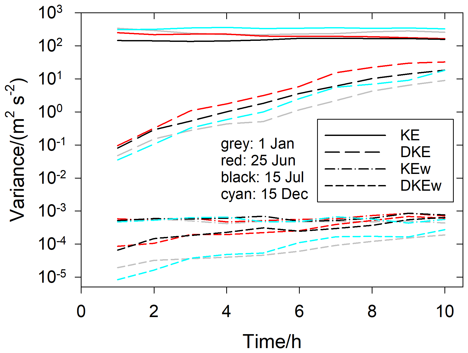
Figure 18 Mean variances of the horizontal and vertical motions (KE and KEw) and related differences (1-way minus 2-way, DKE and DKEw) versus forecast time for four forecasts (different colors) starting at the dates given. The results of the twin experiments are not shown here because they are practically indistinguishable from the contrail runs.

The ecRad radiation solver used in ICON to compute the vertical radiative fluxes and the libRadtran based CoCiP RF model show largely consistent RF results when applied to a homogeneous global cirrus layer. RF is computed in ICON with ecRad by taking the difference between two simulations, with and without contrail coupling. CoCiP provides approximate RF values in the 1-way coupling directly. In order to reduce numerical noise in the ICON results caused by local disturbances, it was important to recalculate the radiation fields at short time intervals and to use the Tripleclouds scheme of ecRad, which is free of random disturbances. The TOA RF values for homogeneous cirrus shown in Fig. 7 have signs as expected from similar studies, but the net RF magnitude is near the lower end of other published results (Myhre et al., 2009; Rap et al., 2010; Ponater et al., 2013; Schumann and Graf, 2013; Schumann and Heymsfield, 2017), possibly because of the size-independent scattering properties of the “Myhre” particles. The RF values from the contrail cases in the first two forecast days in Fig. 14 tend to be higher than the 2021 mean values found in Teoh et al. (2024b) but this comparison suffers from the small set of days considered in this study.

5.2 Coupling effects

As we have seen in the preceding sections, the feedback of contrail properties to the weather forecast model causes changes in the computed contrail properties compared to offline coupling. As expected from earlier studies, the primary effect of contrail formation is a slight reduction of ambient humidity. As a consequence, we find slightly thinner contrails (Figs. 4b, c, and 10). But this effect is smaller than found in earlier studies (Burkhardt and Kärcher, 2011; Schumann et al., 2015). And as expected, the BOA RF is slightly negative with smaller magnitude compared to the TOA RF. Just as thin cirrus clouds (Liou, 1986; Ackerman et al., 1988), contrails warm the ambient atmosphere mainly just below the contrails and cool the stratosphere above the contrails, with a net warming of ambient air (Fig. 15). Within the first 5 d after contrail formation, we see a net warming of ambient air at contrail levels but no systematic change in the global mean Earth surface temperature. Figures 15 and 16 indicate that any expected surface warming due to contrails takes more than 10 d to get notable.

Moreover, we see that the contrail feedback on the background atmosphere causes weather changes nearly immediately at contrail scales and after a few days also at continental scales not equal but similar to random disturbances of the initial conditions. Nonlinear dynamics, in particular from deep convection with strong precipitation, and model parts containing conditional switches (if-statements), enhance the disturbances similarly for contrail and random in initial disturbances. Hence, a different experiment setup is needed to determine significant long-term effects of contrails on the near surface temperature. Perhaps multi-forecast ensemble studies would help in this respect.

Basically, the weak surface warming may be explained by several effects, here listed according to their time scales:

1. The day-mean radiative forcing at bottom of atmosphere is negative, in particular when day-time traffic dominates (Khvorostyanov and Sassen, 1998; Meerkötter et al., 1999).

2. The high water-vapor concentration, aerosols and other clouds below the contrails shield the surface from downward shortwave and longwave fluxes (Meerkötter et al., 1999).

3. The uptake of humidity by contrails causes less cloudiness in the ambient air reducing the contribution of both to surface RF (Burkhardt and Kärcher, 2011).

4. The heating below contrails is not restricted to the air mass vertically below the contrail but spreads horizontally not only at small scales (Gounou and Hogan, 2007; Forster et al., 2012; Unterstrasser et al., 2016) but also at global scales between the northern and southern hemisphere (Ponater et al., 2005).

5. The warming at contrail levels stabilizes the atmosphere below and reduces vertical mixing so that less of the heat induced at contrail levels gets mixed downwards to the surface (Bickel et al., 2025).

6. Only part of the contrail induced heat gets mixed downward to ground since this takes time of order 10 d or longer during which part of the heat gets radiated out to space before it can arrive at the surface (Schumann and Mayer, 2017).

7. The higher pressure of the atmosphere at lower altitudes implies higher heat capacity of the air so that the same amount of flux divergence causes slower heating in the lower atmosphere, increasing the fraction of heat radiated back to space before reaching the surface.

8. In the long term, the surface warming is retarded by the Earth surface and ocean heat capacity (Bickel et al., 2025).

Still, we do expect surface heating to occur after about 10 d, but we do not see this in the present simulations because the nonlinear disturbances hide this heating. This does not exclude significant mean long-term effects, and possibly indirect effects from tropospheric weather changes on the climate system, including precipitation.

As shown above, contrails cause disturbances to weather dynamics, see Fig. 10 etc. Closer inspection of the data details (not presented) shows that the warming of air inside and below contrails induces weak updrafts and local circulations resolved in the numerical model. The disturbances spread quickly horizontally and soon change the atmospheric dynamics in a larger horizontal domain.

Hence, just as weather in general (Feng et al., 2024), contrails are predictable – but only for a finite period. The fact that small disturbances grow with time and spread from small to larger horizontal scales over a few days is a well-known consequence of the nonlinearity of atmospheric dynamics (Lorenz, 1969), but its implications for contrails have not been discussed in detail before. We find that contrails cause butterfly effects similar as described before for other disturbances (Zhang et al., 2003; Rotunno and Snyder, 2008; Selz et al., 2019). Based on spectral analysis (Selz et al., 2019), we find that the initially weak changes at contrail scales grow steadily with time in amplitude and scale (Fig. 17). The spectrum of wind changes reaches the magnitude of the initial kinetic energy of horizontal motions first near the grid or contrail scales and then extends slowly to larger horizontal scales of order 500 km within ten-day forecasts. As a new finding, we note that disturbances in vertical wind reach saturation far earlier than disturbances in horizontal wind. Also, we see that the disturbances grow more quickly in summer under unstable convective conditions than in stable winter weather. One may ask whether the impact of contrails is large enough that its inclusion into numerical weather prediction models might help to improve predictability.

As noted by Selz et al. (2022), random disturbances grow most quickly in areas with convection and, depending on the scales of the disturbances, in areas with horizontal wind divergence and with rotation advection. Kästner et al. (1999) and Gierens and Brinkop (2012) noted that upward and divergent flows favor the formation of ice supersaturation, and ice supersaturation occurs often in anticyclonic flows. Hence, there might be dynamical reasons for why contrails form and persist often in regions where also random disturbances grow most strongly. This is supported by Fig. 14 showing obvious correlations in the ICON TOA and BOA RF responses and in the RF results due to contrails and due to random disturbances. Details deserve further investigations.

As evidenced by Fig. 17, part of the growth of disturbances is caused by the grid discretization and the numerical integration method used in ICON. In addition, although ICON is based on fully compressible equations, we noted super-sonic noise propagation due to the discretization of horizontal diffusion (Zängl et al., 2015), as also seen in other models (Ancell et al., 2018). Moreover, the grid approximations used so far may underrepresent the coupling of the three momentum components by mass conservation, causing checkerboard-noise in the vertical velocity divergence pattern (Korn, 2017) and possibly other disturbances (Langguth et al., 2020; Gassmann, 2021). Hence, though other numerical methods show also strong growth of small-scale disturbances (Ancell et al., 2018; Rodwell et al., 2025), it might be worthwhile to couple CoCiP also to other NWP models to see how far the noise depends on the numerical method used.

The slow response of the surface temperature to contrail RF deserves further investigations. It would be interesting if the coupled ICON–CoCiP model could also be used to determine the long-term climate impact of contrails. So far, this has been achieved using rather coarse models and with either strongly enhanced traffic amounts (Bickel et al., 2025) or with nudging (Gettelman and Chen, 2013). Whether such climate studies are possible with the present approach has still to be shown. In this study we have used a simple twin control setup with random disturbances for causal attribution. In the future, full ensemble simulations with contrails and random disturbances should be considered to extend the quantification of contrail-induced mean changes and their uncertainty and causality.