SO₂ emissions derived from TROPOMI observations over India using a flux-divergence method with variable lifetimes

The rapid development of the economy and the implementation of environmental policies adapted in India have led to fast changes of regional SO₂ emissions. We present a monthly SO₂ emission inventory for India covering December 2018 to November 2023 based on the Tropospheric Monitoring Instrument (TROPOMI) Level-2 COBRA SO₂ dataset, using an improved flux-divergence method and estimated local SO₂ lifetime, which includes both its chemical loss and dry deposition. We update the methodology to use the daily CAMS model output estimates of the hydroxyl-radical distribution as well as the measured dry deposition velocity to account for the variability in the tropospheric SO₂ lifetime. It is the first effort to derive the local SO₂ lifetime for application in the divergence method. The results show the application of the local SO₂ lifetime improves the accuracy of SO₂ emissions estimation when compared to calculations using a constant lifetime. Our improved flux-divergence method reduced the spreading of the point-source emissions compared to the standard flux-divergence method. Our derived averaged SO₂ emissions covering the recent 5 years are about 5.2 Tg yr⁻¹ with a monthly mean uncertainty of 40 %, which is lower than the bottom-up emissions of 11.0 Tg yr⁻¹ from CAMS-GLOB-ANT v5.3. The total emissions from the 92 largest point-source emissions are estimated to be 2.9 Tg yr⁻¹, lower than the estimation of 5.2 Tg yr⁻¹ from the global SO₂ catalog MSAQSO₂LV4. We claim that the variability in the SO₂ lifetime is important to account for in estimating top-down SO₂ emissions.

1 Introduction

Sulfur dioxide (SO₂) is a reactive gas-phase air pollutant released through natural processes, such as volcanic eruptions and passive degassing (Oppenheimer et al., 2011; Carn et al., 2017), as well as anthropogenic activities, primarily from thermal power plants, fossil fuel combustion, and metal smelting and refining (Smith et al., 2011; Klimont et al., 2013; Serbula et al., 2014). After being released into the atmosphere, SO₂ is primarily oxidized in the gas phase by the hydroxyl radical (OH) to form sulfuric acid (H₂SO₄(g)) or scavenged into cloud droplets and subsequential oxidized to form sulfate (SO${}_{\mathrm{4}}^{\mathrm{2}-}$) via the reaction of ozone and hydrogen peroxide (Steinfeld, 1998). Gaseous SO₂ and particulate SO${}_{\mathrm{4}}^{\mathrm{2}-}$ have detrimental effects on human health via increasing the particulate matter concentrations (PM_1.0, PM_2.5). Exposure to SO₂ pollution, whether long or short term, is associated with increased respiratory morbidity (Chen et al., 2007; Clark Nina et al., 2010; Chen et al., 2012; Rodriguez-Villamizar et al., 2015). Sulfuric acid rain induces acidification in both aquatic and terrestrial ecosystems, causing harm to animals and plants (Larssen et al., 2006; Shukla et al., 2013). Additionally, SO${}_{\mathrm{4}}^{\mathrm{2}-}$ contributes to reduced visibility (Leaderer et al., 1979) and acts as a precursor of cloud formation via increasing the cloud condensation nuclei (CCN), subsequently impacting regional and global climate (Lelieveld and Heintzenberg, 1992; Arnold, 2006).

There have been profound changes regarding global anthropogenic SO₂ emissions in the past decades. Specifically, global SO₂ emissions decreased by 31 % between 1990–2015 due to the mitigation efforts in Europe and the USA which have reduced regional SO₂ emissions, while East Asia witnessed a 70 % increase in 1990–2005, followed by a decreasing trend thereafter (Kuttippurath et al., 2022). Contrary to the declining trend in China (Klimont et al., 2013; Li et al., 2017b; Zheng et al., 2018; van der A et al., 2017; Qu et al., 2019), Indian emissions surged from 4.5 to 15.0 Tg S yr⁻¹ between 1990 and 2015 (Crippa et al., 2018; Aas et al., 2019), after which India became the world's largest emitter of anthropogenic SO₂ (Li et al., 2017b, a). Given India's substantial dependence on coal-based thermal power plants to fulfill its growing energy demand, it is anticipated that the emissions will continue to rise driven by population growth and economic development (Venkataraman et al., 2018).

With the development of satellite-based measuring instruments, not only the large SO₂ sources but also the weaker ones can be monitored from space. These satellite measurements provide effective near real-time information, including SO₂ vertical column densities (VCDs) and data quality (QA value), to locate potential SO₂ hot spots and estimate point-source emission terms. During the 1980s, only SO₂ emitted from large volcano eruptions could be monitored from space by the Total Ozone Mapping Spectrometer (TOMS) and the Solar Backscattered Ultraviolet (SBUV) instruments (Krueger, 1983; McPeters et al., 1984; Krueger et al., 2000). After that, the Global Ozone Monitoring Experiment (GOME), launched in 1995, enabled the detection of large industrial SO₂ sources for the first time (Eisinger and Burrows, 1998; Khokhar et al., 2008). Subsequently, the SCanning Imaging Absorption spectroMeter for Atmospheric CHartographY (SCIAMACHY) instrument launched in 2002 (Bovensmann et al., 1999), the Global Ozone Monitoring Experiment-2 (GOME 2) instrument launched in 2006 (Callies et al., 2000), and the Dutch–Finnish Ozone Monitoring Instrument (OMI) instrument launched in 2004 (Levelt et al., 2006) were used to detect sources and monitor emissions from human activities with greater detail (Carn et al., 2007; Lee et al., 2011; McLinden et al., 2016). Half of the reported anthropogenic sources can be detected and quantified with OMI SO₂ measurements (Fioletov et al., 2015, 2016). Nowadays, the Tropospheric Monitoring Instrument (TROPOMI) on the ESA Copernicus Sentinel-5P satellite has become one of the most widely used satellite-based monitoring instruments (Veefkind et al., 2012; Theys et al., 2017). TROPOMI supplies daily global coverage for SO₂ tropospheric vertical column densities (TVCDs) from 2018 to the present. The measurements have a horizontal resolution of approximately 5.5 km × 3.5 km (7 km × 3.5 km before 6 August 2019) at nadir viewing geometry. The TROPOMI SO₂ product reprocessed by the Covariance-Based Retrieval Algorithm (COBRA) has largely reduced the SO₂ noise level and uncertainties as compared to earlier SO₂ datasets derived from TROPOMI or other satellite instruments (Theys et al., 2021). It makes the SO₂ measurements more sensitive to minor SO₂ sources down to 8.0 Gg yr⁻¹(Theys et al., 2021), which indicates that more SO₂ sources can be detected and quantified with the COBRA datasets (Fioletov et al., 2023).

With the significant advancement of satellite-based monitoring instruments over the past decades, a variety of inversion methods have been developed to constrain emissions more efficiently. Data assimilation has been used by combining satellite observations and a chemical transport model (CTM) to derive emissions of trace gases, such as NO_x (Miyazaki et al., 2017; Mijling and van der A, 2012), volatile organic compounds (VOCs; Koohkan et al., 2013), CH₄ (Meirink et al., 2008), and SO₂ (Tsikerdekis et al., 2023). The mass balance method is a less expensive approach for deriving emissions directly from satellite observations without involving a CTM. For example, Leue et al. (2001) and Martin et al. (2003) started to calculate the NO_x emissions based solely on sink terms, ignoring the effect of atmospheric transport. Recently, Fioletov et al. (2011, 2015, 2016, 2023) identified SO₂ point sources using a plume fitting method and quantified emissions based on the mass balance principle with a fixed 6 h effective time. Beirle et al. (2011) used the plume fitting method to derive the NO_x emissions from the large megacity sources and a mean lifetime of NO₂ of 4 h. Later, Beirle et al. (2019) determined the total NO_x emissions using the divergence method, while also calculating point-source emissions using a 2D-Gaussian peak fitting method with a fixed 4 h lifetime. It is noteworthy that the sink term, controlled by the tropospheric lifetime, plays a crucial role in determining the final emission terms according to the mass balance principle. However, previous studies have assumed a constant lifetime for the sink term estimation, which can lead to the spreading of emissions (Beirle et al., 2019). Consequently, deriving realistic local SO₂ lifetimes, which vary from several hours to several days (Chin et al., 2000; Hains et al., 2008; Lee et al., 2011; Green et al., 2019), is crucial to calculate quantitatively accurate SO₂ emissions.

In this study, we will constrain Indian SO₂ emissions for the period December 2018 to November 2023 based on daily TROPOMI SO₂ observations. The flux-divergence method, i.e., combining the independently derived SO₂ sink and divergence, is used to obtain local emissions. Since the sink term is determined by the lifetime, we will initially derive the SO₂ local effective lifetime by incorporating the SO₂ chemical loss and dry deposition. Subsequently, we will improve the divergence method to generate a high-resolution 0.1° × 0.1° emission map, mitigating the smoothing of the emission map. We will estimate the SO₂ emissions using the derived SO₂ local lifetimes and the enhanced divergence method. We then will conduct a comparative analysis with existing bottom-up and top-down emission data. The article is organized as follows: the datasets for the divergence and sink term calculation and SO₂ emissions datasets against which our results are compared are introduced in Sect. 2. Section 3 discusses the basic principles of emission calculation and the method to derive the SO₂ lifetimes. Section 4 illustrates the magnitude of the spreading in the original divergence method and how we reduce this smoothing of the emission map on various spatial resolutions. The uncertainties associated with the resulting SO₂ emission estimates are discussed in Sect. 5. The regional Indian emission estimations, comparisons with respect to existing estimates, and emission changes during the study period are given in Sect. 6. Section 7 discusses the uncertainties which are difficult to quantify. Finally, in Sect. 8 we present our conclusions.

2 Data

2.1 Satellite observations and wind field datasets

TROPOMI on the ESA Copernicus Sentinel-5P satellite was launched on 13 October 2017 (Veefkind et al., 2012). TROPOMI is a hyperspectral nadir sensor consisting of UV–Vis–NIR spectrometers, monitoring key atmospheric species with high accuracy, including NO₂ O₃, SO₂, CH₄, CO, and HCHO as well as aerosol and cloud information. The Sentinel-5P satellite overpass time is about 13:30 local time (LT). The spatial resolution for the center of the swath is approximately 5.5 km × 3.5 km (7 km × 3.5 km before 6 August 2019) in nadir and 5.5 km × 6 km on average over the swath. In this study, the SO₂ emissions are based on the TROPOMI SO₂ product reprocessed by the Covariance-Based Retrieval Algorithm (COBRA) (Theys et al., 2021). The TROPOMI Level-2 COBRA SO₂ data v01.00.01 are extracted from 1 December 2018 to 30 November 2023 for the SO₂ divergence calculation. To ensure the high quality of the measurements, only data with a QA value larger than 0.5 and surface height lower than 3 km are used (https://data-portal.s5p-pal.com/product-docs/so2cbr/S5P-BIRA-PRF-SO2CBR_1.0.pdf, last access: 29 July 2024). Wind field information is needed for the divergence calculation. We used the wind field from the daily operational 12 h forecasts of European Centre for Medium-Range Weather Forecasts (ECMWF) with a resolution of 0.25° × 0.25° (https://www.ecmwf.int/en/forecasts, last access: 29 July 2024). The wind fields are interpolated at the mid-point of the planetary boundary layer (PBL).

2.2 Copernicus Atmospheric Monitoring Service (CAMS) datasets

CAMS has been regularly publishing global forecasts for atmospheric composition from 2015 to present on the ECMWF website (https://ads.atmosphere.copernicus.eu, last access: 29 July 2024) (referred to as the CAMS forecast datasets hereafter). The forecast itself uses ECMWF's Integrated Forecast System (IFS) for the data assimilation and modeling of the concentration of over 50 chemical species (including SO₂ and OH), 7 different types of aerosols, and several meteorological factors provided with a resolution of 0.4° × 0.4°. The CAMS forecast datasets are available for 137 vertical layers with a temporal resolution of 3 h.

Calculating the chemical lifetimes of SO₂ involves deriving a monthly mean OH climatology (derived from 5-year OH concentration as detailed in Sect. 3.2). This climatology is based on the monthly mean OH concentrations accessible within the CAMS forecast datasets. Specifically, the OH concentrations averaged within the PBL at 06:00 UTC (11:30 LT) are used. To ensure a stable OH climatology less influenced by extreme weather events, such as large-scale precipitation occurring on individual days, the monthly mean OH concentrations are averaged over the years from 2018 to 2023. Since cloud cover has minimal influence on the OH concentration over India (Duncan et al., 2024), we did not apply any filtering on OH data based on cloud fraction when computing the OH climatology.

2.3 SO₂ emission and source datasets

Indian SO₂ emissions taken from the bottom-up inventories (i.e., the Emissions Database for Global Atmospheric Research version 8 (EDGARv8) between 2018 and 2022 (Crippa et al., 2024); CAMS global anthropogenic monthly emissions version 5.3 (CAMS-GLOB-ANTv5.3) (Soulie et al., 2024) from 2018 to 2023; and the top-down SO₂ global catalog, the Multi-Satellite Air Quality Sulfur Dioxide (SO₂) database Long-Term L4 Global V2 (referred to as MSAQSO₂L4 hereafter) (Fioletov et al., 2023) from 2019 to 2022) are used for the comparison of the final emission fluxes. The total Indian emissions from CAMS-GLOB-ANT v5.3 and EDGAR v8 show little variation in recent years, about 11.0 Tg yr⁻¹ in each year. The total emissions of India's 92 large point sources from MSAQSO₂LV4 are 5.3, 4.9, 5.2, 5.6 Tg yr⁻¹ during 2019 to 2022, respectively. The locations of Indian thermal power plants we use in this study originate from the Open Infrastructure Map (https://openinframap.org/stats/area/India, last access: 29 July 2024).

3 Method description

This flux-divergence method is initially proposed by Beirle et al. (2019) and has been refined and applied in estimating emissions of trace gases like NO_x (Beirle et al., 2021) and CH₄ (Liu et al., 2021). Here we apply it for the derivation of SO₂ emissions. The steady-state equation governing the flux-divergence method is described as follows:

$$\begin{array}{}\text{(1)}& E=D+S,\end{array}$$

with D, E. and S being the terms of divergence, emission. and sink of SO₂, respectively. This equation shows that the SO₂ emissions are obtained by adding estimates of SO₂ divergence and sink terms. The two main steps, the divergence calculation and the sink calculation, are discussed below.

3.1 Calculation of the divergence

Equation (2) defines divergence (D) as the continuity equation of the flux (F), incorporating SO₂ VCDs (V) and wind field data (w):

$$\begin{array}{}\text{(2)}& D=\mathrm{\nabla }\cdot \mathit{F}=\mathrm{\nabla }\left(\mathit{w}\cdot V\right).\end{array}$$

Note that because both VCDs and wind information are available on a grid scale rather than a continuous state, the second-order central finite difference method (SOCFDM) is used to approximate the divergence. The daily divergence of a grid cell needs to be derived for both x and y directions (see the one-dimensional example in the Supplement).

3.2 Calculation of the sink term

The relation between sink term, atmospheric density, and lifetime can be expressed as

$$\begin{array}{}\text{(3)}& S={\displaystyle \frac{V_{{\mathrm{SO}}_{\mathrm{2}}}}{\mathit{\tau }}},\end{array}$$

with S the SO₂ sink term, $V_{{\mathrm{SO}}_{\mathrm{2}}}$ the SO₂ VCD, and τ the SO₂ effective lifetime. The SO₂ VCDs are taken from the satellite measurements. The SO₂ lifetime is determined by various processes in the atmosphere responsible for removing SO₂, including deposition and chemical loss. As the deposition and chemical loss occur simultaneously, the SO₂ effective lifetime τ is defined as follows:

$$\begin{array}{}\text{(4)}& {\displaystyle \frac{\mathrm{1}}{\mathit{\tau }}}={\displaystyle \frac{\mathrm{1}}{{\mathit{\tau }}_{\mathrm{c}}}}+{\displaystyle \frac{\mathrm{1}}{{\mathit{\tau }}_{\mathrm{d}}}},\end{array}$$

where τ_c is the chemical lifetime, and τ_d is the lifetime related to SO₂ dry deposition.

3.2.1 Calculation of the chemical lifetime

Notably, TROPOMI can “see” SO₂ only in the cloud-free part of the pixel, leaving SO₂ concentrations within or beneath clouds being unmeasurable. We assume that the resulting SO₂ has had no interaction with clouds; thus the resulting lifetime derived for SO₂ pertains to cloud-free conditions in a constrained region. Oxidization by OH(g) determines the SO₂ chemical lifetime in the atmosphere under cloud-free conditions (Blitz et al., 2003; Long et al., 2017; Green et al., 2019). This reaction occurs primarily during daytime hours with maximum sunlight under humid conditions. Considering the TROPOMI overpass time is 13:00 LT, coinciding with peak OH concentrations and favorable conditions for the SO₂ + OH reaction, we assume SO₂ lifetime dominance via OH oxidation. Therefore, we use the model-simulated OH concentration at 11:30 LT, which is closest to the TROPOMI overpass time from CAMS forecast datasets, to calculate the chemical lifetime τ_c (s⁻¹) as follows:

$$\begin{array}{}\text{(5)}& {\mathit{\tau }}_{\mathrm{c}}={\displaystyle \frac{\mathrm{1}}{k\left[\mathrm{OH}\right]}},\end{array}$$

with k being the chemical rate coefficient (molec.⁻¹ cm³ s⁻¹) and [OH] denoting the OH concentration (molec. cm⁻³), i.e., OH column density, within the PBL divided by the PBL height. The rate coefficient k depends on the atmospheric temperature and is calculated following Table 2-1 in Vladimir et al. (2015). Due to the OH concentrations exhibiting a clear seasonal cycle (Lelieveld et al., 2016), we derive a monthly OH climatology (December 2018 to November 2023) and calculate k to estimate the SO₂ chemical lifetime per month per grid cell as shown in Fig. S1. The estimated SO₂ monthly mean chemical lifetime varies from 16 to 34 h. While the distribution of the SO₂ chemical lifetime does not show big differences within the same season, it has a clear seasonality, with the lowest chemical lifetime occurring in summer and the highest in winter. The chemical lifetimes averaged for the whole of India in winter, spring, summer, and autumn are 31, 18, 16, and 22 h, respectively. The variation in SO₂ chemical lifetime is also notable across various regions. The SO₂ chemical lifetime in northern regions is larger than that in the south, with an exception occurring in summer when there is less spatial variation in lifetime. This is because more OH can be generated at low latitudes in the lower to middle troposphere due to the small solar zenith angle and high concentration of water vapor (Crutzen and Zimmermann, 1991; Spivakovsky et al., 2000). As these papers show, the OH concentration near the Equator remains consistently high throughout all seasons, leading to less variable chemical lifetimes in southern India compared to the north (Fig. S1).

3.2.2 Deposition lifetime

Wet and dry deposition influences the SO₂ lifetime in the atmosphere. However, given that all SO₂ is measured in cloud-free areas, our analysis only considers the impact of dry deposition, i.e., direct loss to the surface. Previous studies have indicated that SO₂ dry deposition lifetimes span several days (Matsuda et al., 2006; Faloona et al., 2009; Hayden et al., 2021). Here we use 0.4 cm s⁻¹ as a general dry deposition velocity, which is based on measurements from Hicks (2006), Myles et al. (2007), and Faloona et al. (2009). The SO₂ monthly dry deposition lifetime within the PBL height is calculated by dividing the PBL height (from ECMWF data) by 0.4 cm s⁻¹ (Slinn et al., 1978). As shown in Fig. S2, the Indian SO₂ monthly mean dry deposition lifetime varies from 55 to 135 h, with the longest lifetime occurring in spring. The dry deposition lifetimes averaged over the whole of India in winter, spring, summer, and autumn are 62, 120, 75, and 70 h, respectively. The lifetime is longer in spring due to the higher PBL in this season.

3.2.3 The SO₂ effective lifetime

Following Eq. (4) we combine the SO₂ chemical lifetime and dry deposition terms to calculate the SO₂ monthly effective lifetime for each grid cell to derive the local sink term. The SO₂ monthly mean effective lifetime in India varies from 12 to 19 h (Fig. S3). Figure 1 displays SO₂ effective lifetimes averaged for each season. The SO₂ seasonal mean lifetimes averaged for India in winter, spring, summer, and autumn are 19, 15, 12, and 16 h, respectively. After considering the SO₂ dry deposition, the annual mean SO₂ effective lifetime decreases by 27 % compared to only considering the chemical loss, reducing the fraction transported away from strong point sources. Comparing the SO₂ lifetime derived here with the lifetimes proposed in the literature shows that our estimates are similar to other independent model-based lifetime estimates (Lee et al., 2011) and ground-measurement-based lifetime estimates (Hains et al., 2008). We therefore argue that on average our calculated SO₂ lifetime is reasonable. Furthermore, it has a latitude and seasonal dependency that is often lacking in other inversion methods.

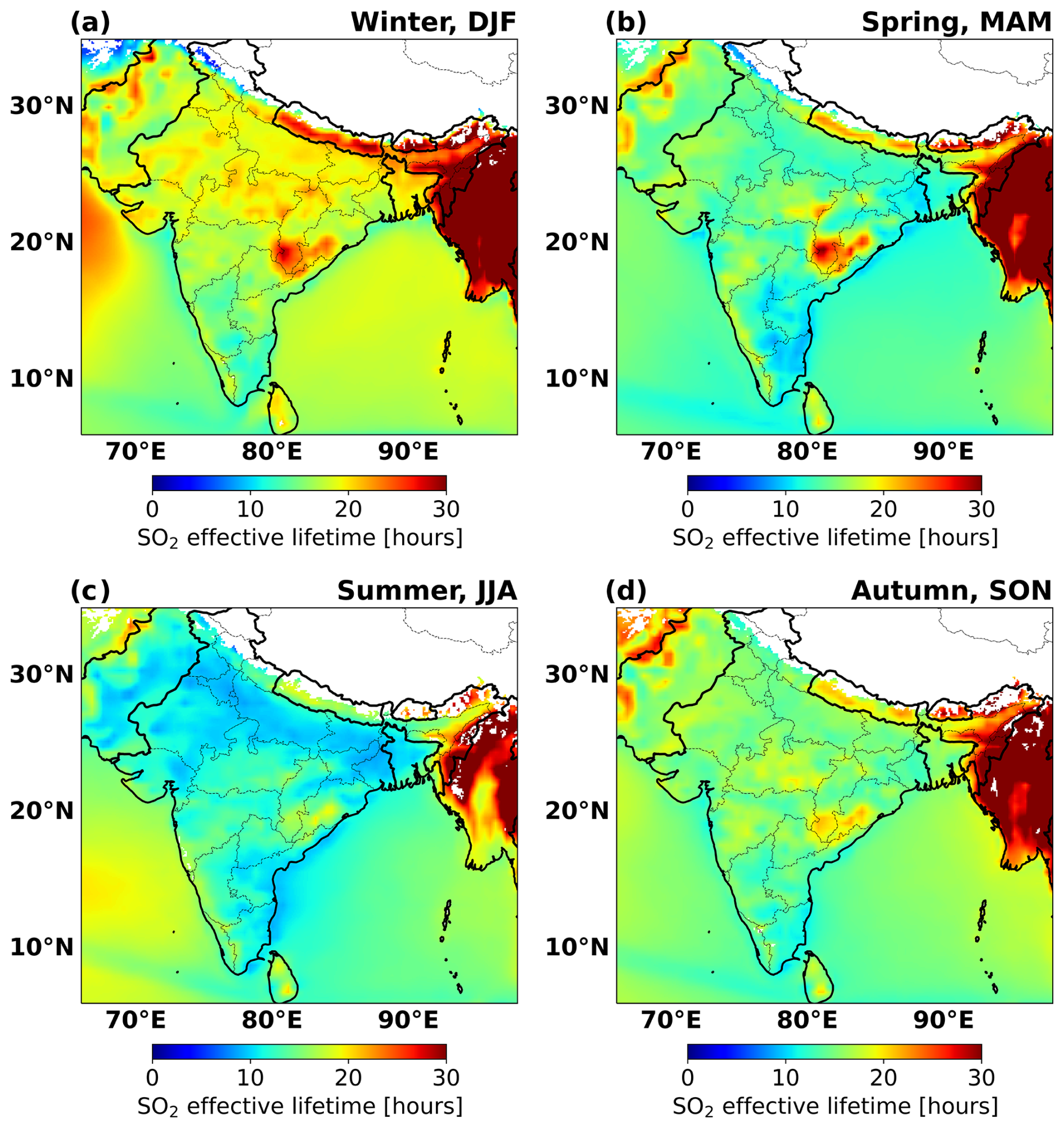
Figure 1 SO₂ seasonal mean effective lifetime in India. Lifetime in each season is averaged for the period from December 2018 to November 2023. (a) Winter DJF: December–January–February. (b) Spring MAM: March–April–May. (c) Summer JJA: June–July–August. (d) Autumn SON: September–October–November. The white region represents the areas with surface heights larger than 3 km or the areas without high-quality SO₂ measurements. These regions are not discussed in this study.

3.2.4 The SO₂ effective lifetime validation

The monthly mean SO₂ effective lifetime is calculated based on OH oxidation and the SO₂ dry deposition. We assume negligible influence on lifetime from SO₂ wet deposition and other chemical reactions occurring in the cloud's droplets in terms of monthly mean lifetime, especially since we use only cloud-free observations. To show this, we derive a monthly mean SO₂ lifetime ($\stackrel{\mathrm{‾}}{\mathit{\tau }}$) from the CAMS model by considering all SO₂ producing processes and all kinds of sink according to Eq. (6),

$$\begin{array}{}\text{(6)}& \stackrel{\mathrm{‾}}{\mathit{\tau }}={\displaystyle \frac{C}{E}},\end{array}$$

with C being the total SO₂ concentration and E the total SO₂ emissions. We sum both the concentrations and the emissions of the model for each month covering the whole of India to derive a monthly mean averaged C and E for the whole of India. Figure 2 shows the monthly $\stackrel{\mathrm{‾}}{\mathit{\tau }}$ in 2019–2020 and 2022–2023 based on the CAMS model. This model-intrinsic SO₂ lifetime of each month consistently exceeds 7 h. The lowest lifetime is in summer, around 9.5 h on average, while the longest lifetime is in winter, around 25.5 h on average. The lifetime in spring and autumn is comparable, around 19 h on average. Note that the CAMS model includes both dry and wet deposition of SO₂. The noticeable monthly/seasonal variation of lifetime aligns well with our calculations based on the OH oxidation and SO₂ dry deposition, indicating our calculated SO₂ lifetime will not change significantly, even if wet deposition and other chemical reactions are considered now. At the same time, we see a large variation both spatially and in the average from month to month. Therefore, we will use the monthly averaged local lifetime from here on.

Figure 2 Monthly averaged SO₂ lifetime in India for (a) 2019–2020 and (b) 2022–2023. The lifetime is calculated by accounting all SO₂ producing processes and all kinds of sink in the CAMS model.

3.3 Emission calculation

The final emission term is the sum of the flux-divergence term and the sink term and can be expressed as

$$\begin{array}{}\text{(7)}& \begin{array}{rl}E& =D+S=\mathrm{\nabla }\left(\mathit{w}\cdot V_{{\mathrm{SO}}_{\mathrm{2}}}\right)+{\displaystyle \frac{V_{{\mathrm{SO}}_{\mathrm{2}}}}{\mathit{\tau }}}\\ & =\mathit{w}\cdot \mathrm{\nabla }\left(V_{{\mathrm{SO}}_{\mathrm{2}}}\right)+V_{{\mathrm{SO}}_{\mathrm{2}}}\cdot \mathrm{\nabla }\left(\mathit{w}\right)+{\displaystyle \frac{V_{{\mathrm{SO}}_{\mathrm{2}}}}{\mathit{\tau }}},\end{array}\end{array}$$

where $\mathit{w}\cdot \mathrm{\nabla }\left(V_{{\mathrm{SO}}_{\mathrm{2}}}\right)$ is the flux divergence of the SO₂ concentrations, $V_{{\mathrm{SO}}_{\mathrm{2}}}\cdot \mathrm{\nabla }\left(\mathit{w}\right)$ is the wind divergence, and the last term describes the sink. The wind divergence term considers the vertical transport, which contributes to the divergence of the wind and can affect the calculated emissions. To calculate this wind divergence term, we follow the method described in Bryan (2022) to remove the wind divergence from the equation. To minimize the impact of noise on the SO₂ measurements, we average the divergence over each season. Emissions for each month are then calculated by summing the monthly sink term and the divergence term of the corresponding season. The divergence calculation can be conducted on different spatial scales. Given the target resolution for the emissions is 0.1° × 0.1°, the divergence calculation can be conducted on a 0.1° × 0.1° regular grid cell (which corresponds to an approximate surface area of 10 km × 10 km) after integrating the measured SO₂ VCDs to the regular grid cells. Since the emission map resolution is limited by the pixel scale of TROPOMI, we also calculate the divergence based on the original TROPOMI-measured pixels (on an along- × cross-track grid, about 5.5 km × 3.5 km at nadir varying with the viewing angle) (de Foy and Schauer, 2022) and later integrate the divergence to the regular grid cells of 0.1° × 0.1°. The integration from the TROPOMI pixels to regular grid cells is based on the weight of the overlap areas. The divergence calculations on different spatial resolutions mentioned above are conducted in this study. The final emissions are calculated from the divergence map with the best performance.

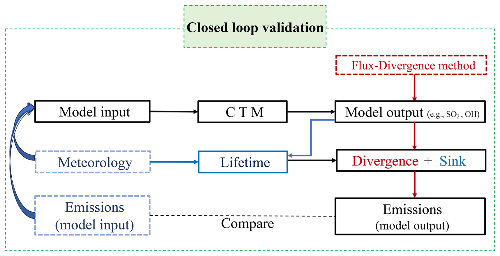
3.4 Closed-loop validation approach

To verify both the flux-divergence method and the derived OH climatology, we have tested our method using the simulated data from CAMS forecast datasets with the known input emissions CAMS-GLOB-ANT v4.2 (Fig. 3). We use the simulated SO₂ VCDs within the PBL and the wind field at the mid-point of the PBL from the CAMS forecast datasets (0.4° × 0.4°) from December 2019 to November 2020 to calculate the CAMS top-down SO₂ emissions with the flux-divergence method, in which the sink term is calculated following Sect. 3.2. The CAMS-GLOB-ANT v4.2 data (Soulie et al., 2024), which are applied in the CAMS forecast datasets across 2019/2020, are used for comparison with the CAMS top-down SO₂ emissions. If they align closely, it indicates that the lifetime and flux-divergence method work well in this process.

Figure 3 Illustration of the closed-loop validation.​​​​​​​

4 Improvement of the flux-divergence calculation

To verify the performance of the flux-divergence method, it is initially tested in a closed-loop validation to calculate the CAMS top-down SO₂ emissions with a resolution of 0.4° × 0.4°. Figure 4a shows the model input emissions (CAMS-GLOB-ANT v4.2), and Fig. 4b shows the CAMS top-down SO₂ emissions derived with the original flux-divergence method (hereafter referred to as the classic divergence method (CDM)). The total CAMS top-down SO₂ emissions for the Indian domain are 15.0 Tg yr⁻¹, close to 13.6 Tg yr⁻¹ calculated in the CAMS-GLOB-ANT v4.2. However, the distribution differences between the two maps are significant. The map of Fig. 4a shows a more distinct emission signal at precise locations representing point sources, whereas the emission map from Fig. 4b shows a noticeable spreading effect of point sources. This effect leads to a large difference in the emissions at the source locations. The spreading effect in the emissions derived with the CDM is a result of using the SOCFDM to approximate the continuity equation of the divergence calculation (Eq. 1), since it effectively involves a linear interpolation. To show this, Eq. (1) used to calculate the divergence in grid cell i along x direction can be rewritten as

$$\begin{array}{}\text{(8)}& D_{x\left(i\right)}={\displaystyle \frac{\mathrm{1}}{\mathrm{2}}}\left[{\displaystyle \frac{\left({\mathit{F}}_{x(i+\mathrm{1})}-{\mathit{F}}_{x\left(i\right)}\right)}{\mathrm{\Delta }x}}+{\displaystyle \frac{\left({\mathit{F}}_{x\left(i\right)}-{\mathit{F}}_{x(i-\mathrm{1})}\right)}{\mathrm{\Delta }x}}\right].\end{array}$$

Here, F_x(i) denotes the flux of SO₂ in grid cell i along the x direction, and Δx is the resolution of the grid-scale data. Then, the divergence in grid cell i along x direction can be expressed as

$$\begin{array}{}\text{(9)}& D_{x\left(i\right)}={\displaystyle \frac{\mathrm{1}}{\mathrm{2}}}\left[D_{\mathrm{RE}\left(i\right)}+D_{\mathrm{LE}\left(i\right)}\right],\end{array}$$

with D_RE(i) and D_LE(i) representing the divergence at the right edge and the left edge of grid cell i. Thus, the divergence of each grid cell is essentially a linear interpolation of the divergence at the grid cell edges. If we perceive the divergence interpolation as a divergence allocation, the linear interpolation of the divergence essentially means that half of the divergence is allocated to the source location grid cell, while the remaining half is allocated to the grid cell adjacent to the source location grid cell, resulting in the spreading effect (Fig. S4c).

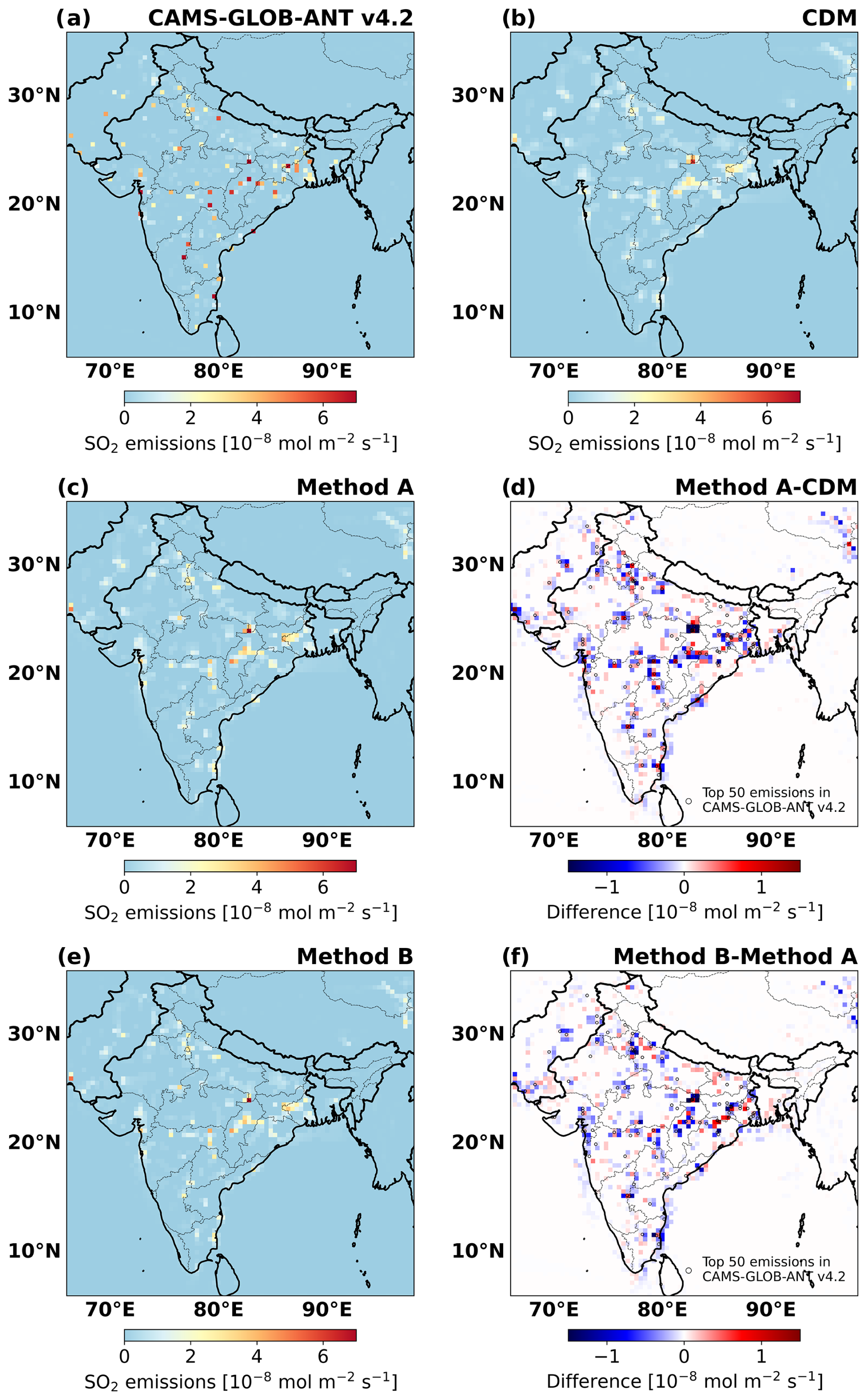
Figure 4 The CAMS model input and CAMS top-down SO₂ emission distribution in the winter season (December–January–February) of 2019/2020. The emissions from (a) the CAMS-GLOB-ANT v4.2 inventory and emissions derived with (b) the CDM, (c) method A, and (e) method B are shown. Panel (d) shows the difference in emissions between the CDM and method A. Panel (f) shows the difference in emissions between the CDM and method B. The black circles represent the locations of the top 50 emissions in the CAMS-GLOB-ANT v4.2 inventory.

As the spreading is a result of the discrete steps in SOCFDM, the improvements mainly focus on using different divergence interpolation/allocation methods to reduce the spreading and make the emission signals “sharper” in the source locations. In the one-dimensional situation along the wind, the highest SO₂ concentration occurs downwind of the source (Fig. S4b). The largest SO₂ VCD gradient is displayed around the source, especially upwind (Fig. S4a). Considering this distribution, we conduct method A, assigning all of the edge divergence to the grid cell, whose opposite edge has the larger SO₂ VCD gradient (see formula in Sect. S5 in the Supplement). Figure 4c using method A shows that the spreading effect is reduced efficiently compared to Fig. 5b using the CDM. The most notable improvements are observed in the source locations, suggesting that method A can yield a higher-quality emission inventory. However, compared to the input emissions used in CAMS and shown in Fig. 5a, method A still shows a clear spreading effect. Although method A is very effective in a theoretical one-dimensional example, it is much less efficient in two dimensions, where the grid cells and wind direction (i.e., the plume) are usually not aligned. The highest SO₂ concentration downwind of the source can be dispersed across multiple grid cells in the two-dimensional situation. Therefore, the peak concentration usually occurs at the source location (See Fig. S5). Based on this, we have developed a more advanced methodology (hereafter referred to as method B), which allocates all of the edge divergence to the grid cell with the larger SO₂ VCD (See formula in Sect. S6 in the Supplement). The emission map derived with method B provides better results when compared to the CDM as shown in Fig. 5f and method A as shown in Fig. S6b. It is noteworthy that only the distribution is different between emissions derived with the CDM, method A, and method B. The total amount of SO₂ emissions derived with the different methods remains the same. This is because the total divergence over the domain equals zero, and the total emission amount is solely determined by the SO₂ sink term. We subsequently adopt method B to calculate divergence at the resolution of 0.1° × 0.1° (about 10 km × 10 km) and at the original TROPOMI-measured pixels (along × cross, about 5.5 km × 3.5 km at nadir), respectively. The divergence of the TROPOMI-measured pixels are also gridded to 0.1° × 0.1° afterwards. From Fig. 5 we see that emissions from point sources derived from the TROPOMI-measured pixels are more convergent to the point-source location (less smoothing), although the background noise also seems enhanced. For each test, method B shows emission maps with a higher spatial resolution than the other methods. Considering the outcome of these tests, our calculated emissions will be based on the divergence on TROPOMI-measured pixels derived with method B. For emissions of an individual point source (e.g., a power plant), we will sum all emissions in the 5 × 5 grid cells around the point source because part of the spreading effect still remains in the results.

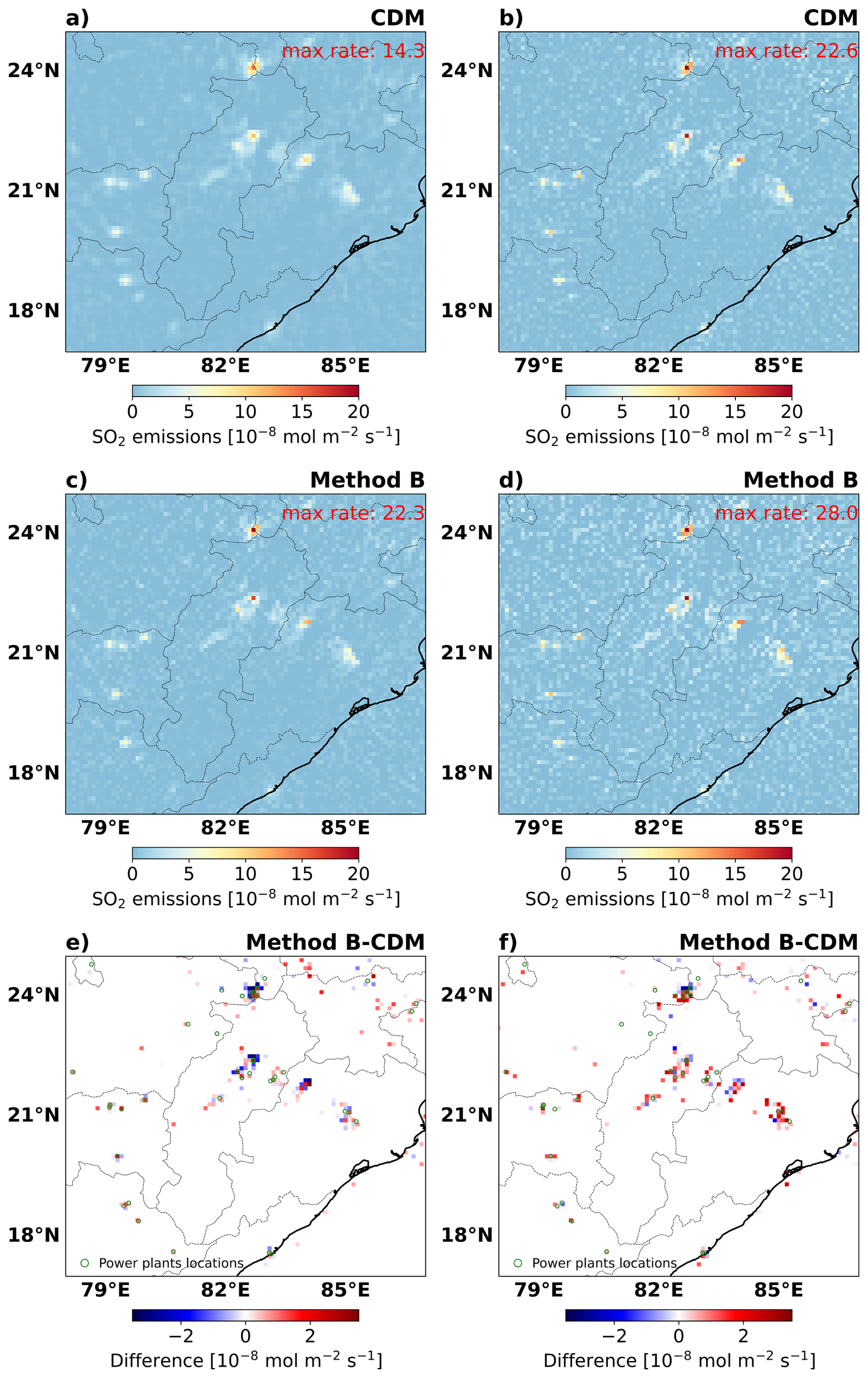
Figure 5 The SO₂ emission distribution in the winter season (DJF) of 2019/2020 in a selected domain (17–25° N, 78–87° E) with large thermal power plants (a–d). The emissions (a, c) are derived from the divergence calculated directly on a 0.1° resolution using the CDM (a) and method B (c). (b, d) Emissions are derived based on the divergence calculated on the TROPOMI-measured pixels using the CDM (b) and method B (d). (e, f) The difference in emissions between method B and the CDM (method B − CDM) and for the divergence calculated directly on 0.1° resolution (e) and derived on the TROPOMI-measured pixels (f). The green circles represent the locations of thermal power plants with annual power generation larger than 1000 MW (from Open Infrastructure Map, https://openinframap.org/stats/area/India).

5 Uncertainty assessment

As the uncertainty is mainly determined by the sink term, the SO₂ emissions uncertainty involves the uncertainties from the measured SO₂ VCDs and those associated with the SO₂ effective lifetime, of which the latter are primarily related to the OH concentrations and dry deposition velocity. The SO₂ VCD uncertainty is mainly from the calculation of air mass factors (AMFs). Here we apply an averaged AMF uncertainty of about 30 % for the individual measurement column, which is estimated from the S5P/TROPOMI SO₂ ATBD file (https://sentinel.esa.int/documents/247904/2476257/Sentinel-5P-ATBD-SO2-TROPOMI, last access: 29 July 2024). Considering there are 17 effective measurements on average for each month across India, the uncertainty from AMFs for monthly mean SO₂ VCDs is calculated to be about 7 % $\left(\frac{\mathrm{30}\mathit{\%}}{\sqrt{\mathrm{17}}}\right)$. The uncertainty associated with the dry deposition velocity only has a second-order effect on the SO₂ effective lifetime, with the uncertainty in the OH term dominating. If the dry deposition velocity increases by 100 %, the effective lifetime for SO₂ is only reduced by 20 %. Since there is a lack of validation of OH concentration due to a scarcity of measurements, we assume the differences of the simulated OH by the IFS model with various chemistry schemes (IFS(CB05BASCOE), IFS(MOZART), IFS(MOCAGE)) as an estimate of the OH uncertainty, which can reach up to 50 % (Huijnen et al., 2019). Changes in the OH density by ±50 % generally translate to a maximum uncertainty of 60 % increase or a 20 % decrease in SO₂ effective lifetime. Consequently, the uncertainties of Indian emissions mainly involve the uncertainties from SO₂ VCDs and from the CAMS OH concentrations. Combining the uncertainties leads to an emission uncertainty ranging from a maximum of −42 % to +33 %. Although the measured SO₂ plume has no interaction with the clouds during the TROPOMI overpass, the SO₂ may interact with clouds before and after this time to influence the effective SO₂ lifetime. Therefore, we take an uncertainty of 40 %, which is larger than the averaged uncertainty (35 %), for SO₂ monthly emissions.

6 Results

6.1 Calculation of the SO₂ emissions and the emission detection threshold

We calculate annual SO₂ emissions over India for the period December 2018 to November 2023 (5 years). The 5-year-averaged annual SO₂ emission map in Fig. 6a effectively captures large emission hot spots. But the noise on the data hampers precise differentiation of the weakest SO₂ point sources. To address this, we assess the noise level on the measurement or the emission detection threshold from a selected ocean region (within 5–18° N and 85–90° E), which typically contains no strong ship or other emissions. The frequency distribution of annual SO₂ emissions (or background noise) within the selected region approximates a normal distribution with σ = 0.52 Gg yr⁻¹ as depicted by the blue bars in Fig. S7. We define the detection threshold as 4 times σ (about 2.0 Gg yr⁻¹ per grid cell). The emissions sources above the detection threshold are shown in Fig. 6b–d. It displays a good location alignment with the source locations detected in MSAQSO₂LV4 and the known thermal power plants.

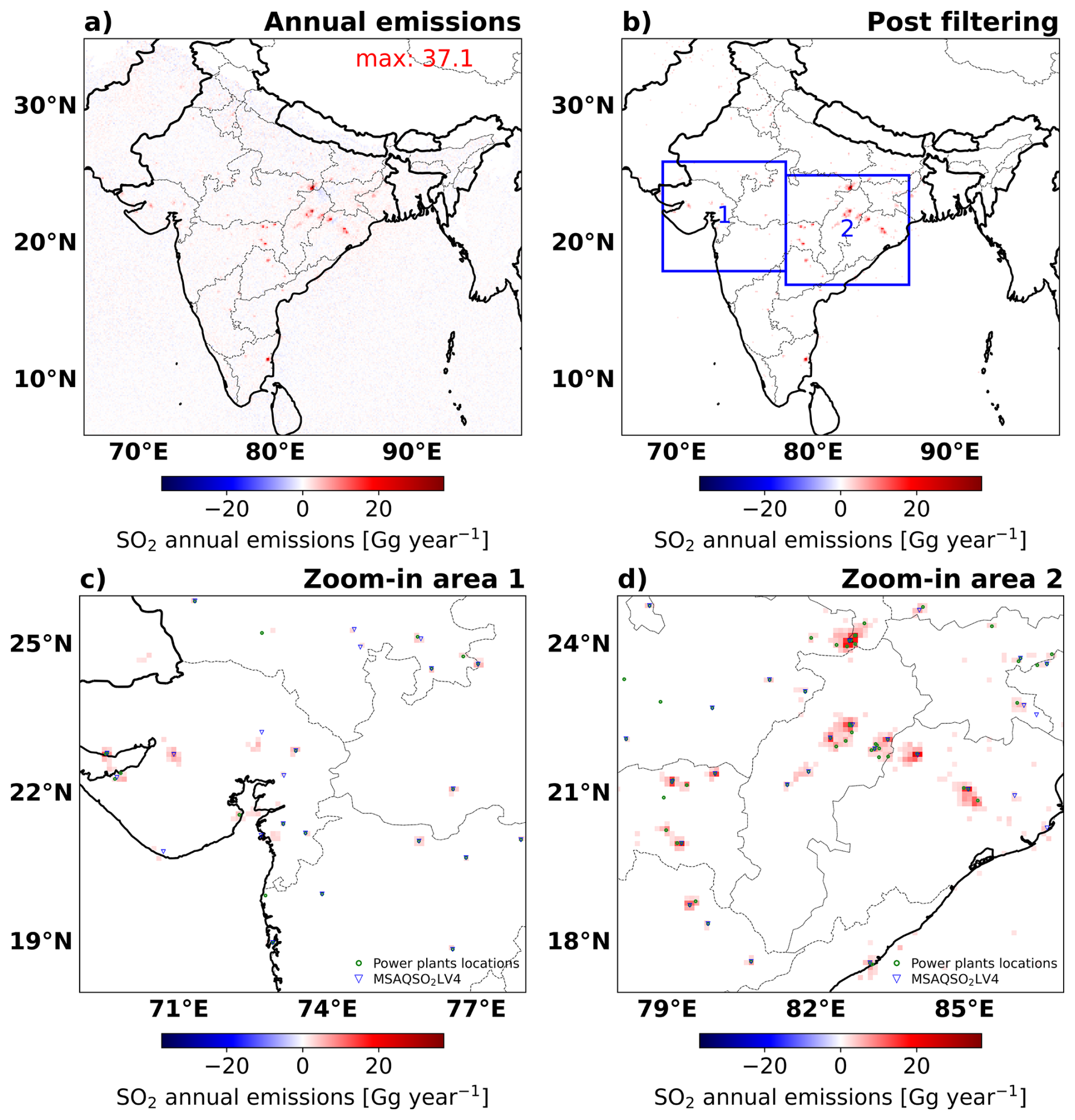
Figure 6 (a) The SO₂ annual mean emissions averaged between December 2018 to November 2023. Panel (b) shows the emissions above the detection threshold of 2.0 Gg yr⁻¹. Panels (c) and (d) show the emissions of the zoomed-in views of area 1 and 2, respectively. The blue triangles represent the source locations identified by MSAQSO₂L4. The green circles represent the locations of thermal power plants with annual power generation larger than 500 MW from the Open Infrastructure map (https://openinframap.org/stats/area/India). The range of the color bar is scaled with the maximum value.

The annual mean emissions for the whole of India from December 2018 to November 2023 are approximately 5.7, 4.2, 5.1, 5.1, and 5.7 Tg yr⁻¹, with the 5-year-averaged SO₂ emissions being 5.2 Tg yr⁻¹, with an uncertainty of ±12 % $\left(\frac{\mathrm{40}\mathit{\%}}{\sqrt{\mathrm{12}}}\right)$. The sudden reduction in SO₂ emissions in 2020 corresponds to the declining trend of coal consumption in the same year (IEA, 2023) likely due to the effects of the COVID-19 pandemic on energy consumption (Levelt et al., 2022). The Indian SO₂ emissions show a seasonality: the emissions in winter (DJF) are on average 0.50 Tg per month, in spring (MAM) 0.57 Tg per month, in summer (JJA) 0.25 Tg per month, and in autumn (SON) 0.41 Tg per month. During the summer season more additional power capacity from hydropower and wind power is available (related to the monsoon), and less energy from coal powerplants is needed (IEA, 2023).

6.2 Comparison against other Indian SO₂ emissions datasets

We compare our SO₂ emission fluxes against those taken from the global catalog MSAQSO₂L4 for 92 strong SO₂ point sources. The total SO₂ emissions of 92 point sources averaged over 5 years are 2.9 Tg yr⁻¹, notably lower than 5.2 Tg yr⁻¹ in MSAQSO₂L4. The scatter plot in Fig. 7 shows the annual emissions averaged over the 5-year study period. The strong and significant correlation (P < 0.05) between the two emission datasets results in a Pearson R value of 0.87, confirming the efficiency and accuracy of the divergence method for detection of strong point sources. To further explore the differences in these emissions terms depicted in Fig. 7a, we also calculate the emissions assuming a constant SO₂ lifetime of 6 h assumed in MSAQSO₂L4 by Fioletov et al. (2023). This adjustment increases our SO₂ emissions to 4.0 Tg yr⁻¹, which is closer to the total emissions of the MSAQSO₂L4 (Fig. 7b). But we see a noticeable smoothing effect and an overall positive bias on emissions estimated with a fixed 6 h lifetime compared to the emissions estimated with a local, variable lifetime, especially around the source location (Figs. 7c, d and S8). This indicates that the lifetime of 6 h is too short, and the application of a non-constant SO₂ lifetime to constrain SO₂ emissions is more realistic. Consequently, we suggest that the real SO₂ emissions in India are lower than emissions estimated with a fixed 6 h lifetime.

Figure 7 (a) Comparison between SO₂ emissions in this study derived using a variable lifetime (x axis) and the corresponding SO₂ emissions from the MSAQSO₂LV4 catalog (y axis). (b) Same as panel (a) but for emissions derived with a 6 h lifetime on the x axis. (c) SO₂ emissions derived with the non-constant lifetime. (d) Same as panel (c) but for emissions derived with a 6 h lifetime. The point-source emissions from MSAQSO₂LV4 are averaged from 2019 to 2022. The emissions from this study are averaged from December 2018 to November 2023.

To further compare the emissions to other inventories, we select our top 10 highest emission sources (see locations in Fig. S9). Our top 10 sources are associated with thermal power stations, emitting in total 1.1 Tg yr⁻¹, which accounts for 21 % of all SO₂ emissions in India. The comparison with the global catalog MSAQSO₂LV4 and the bottom-up emission inventories, EDGAR v8 and CAMS-GLOB-ANT v5.3, is shown in Fig. 8. Generally, the emissions from our top 10 sources are lower than those reported by the other inventories. Except for Chandrapur (20.01° N, 79.29° E) and Durgaphur (23.55° N, 87.21° E), our top 10 sources are also listed in the Indian top 10 sources from MSAQSO₂LV4. The largest emitter, Vindhyachal, representing 5 × 5 grid cells around the Vindhyachal Superpower Station (24.9° N, 82.68° E), is also the largest SO₂ emission source in CAMS-GLOB-ANT v5.3 and EDGAR v8. Neyveli (11.55° N, 79.44° E) is the largest SO₂ emitter in the MSAQSO₂L4 and is the third largest in our inventory. Within the 5 × 5 grid cells of Neyveli, several coal power plants are situated near a lignite mine. Our comparison of the highest emitter (Neyveli) in Fig. 7a and b indicates that the emission disparities between our inventory and MSAQSO₂L4 cannot be solely attributed to different lifetimes, suggesting that the choice of inversion method can also play a key role in constraining emissions.

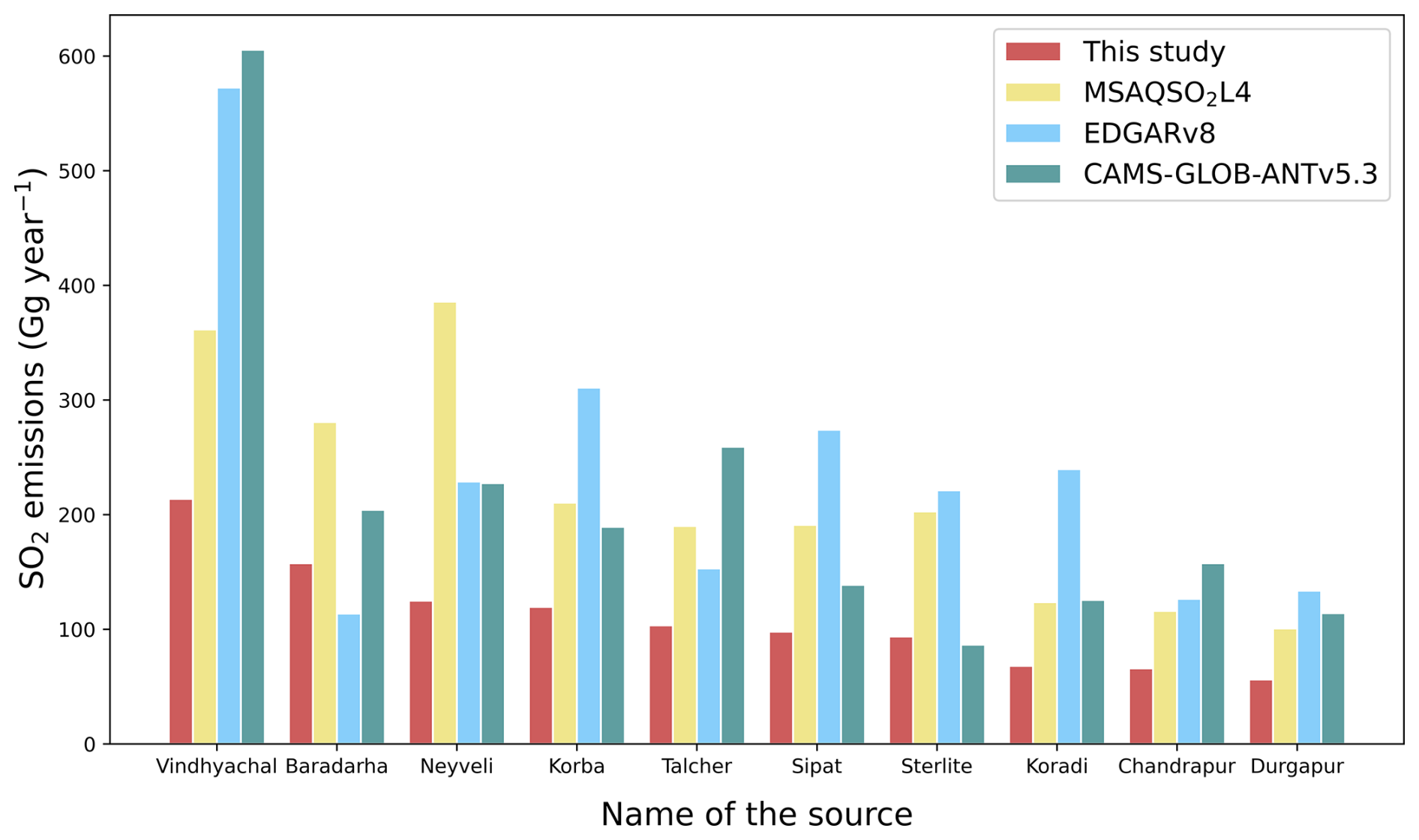
Figure 8 A comparison of SO₂ emission estimates from our 10 largest point sources in India using the global catalog MSAQSO₂LV4, EDGAR v8, and CAMS-GLOB-ANT v5.3 datasets. The sources are sorted by descending order of our emissions. The x label lists the name of each source (i.e., power plant). For the inventories, the total emissions within 5 × 5 grid cells centered by the source location are used for comparison. Emissions from MSAQSO₂LV4 are averaged from 2019 to 2022. Emissions from EDGAR v8 are averaged from December 2018 to November 2022. Emissions from other inventories are averaged from December 2018 to November 2023.

We calculate Indian SO₂ emissions to be 5.2 Tg yr⁻¹ using the SO₂ local lifetime and 12.0 Tg yr⁻¹ using a fixed 6 h lifetime. The country-total emissions obtained with a local lifetime are about 50 % lower than the reported emissions in the most used bottom-up inventories, i.e., CAMS-GLOB-ANT and EDGAR. The CAMS-GLOB-ANT v5.3 inventory estimates that India emitted 11 Tg yr⁻¹ SO₂ in 2023. However, the CAMS-model-simulated SO₂ densities, driven by CAMS-GLOB-ANT v5.3, are much higher (by a factor of 2) than the TROPOMI measurements (see the comparison for 2023 in Fig. 9). The emissions at the large source locations show big differences between the two maps. Many strong source signals in the west of India are shown on the CAMS map, while they are not visible on the TROPOMI map. Considering the good data quality of the TROPOMI observations (Theys et al., 2021; De Smedt et al., 2021), we suggest that the difference in Fig. 9 is primarily due to a positive bias in model input emissions. It is noted that the SO₂ lifetime in CAMS model may be overestimated and contribute to the higher simulated SO₂ concentration, even though the OH level, which mainly determines the SO₂ lifetime under cloud-free conditions, is similar between CAMS results (Fig. S10) and the previous studies (Hewitt and Harrison, 1985; Lelieveld et al., 2004; Souri et al., 2024).

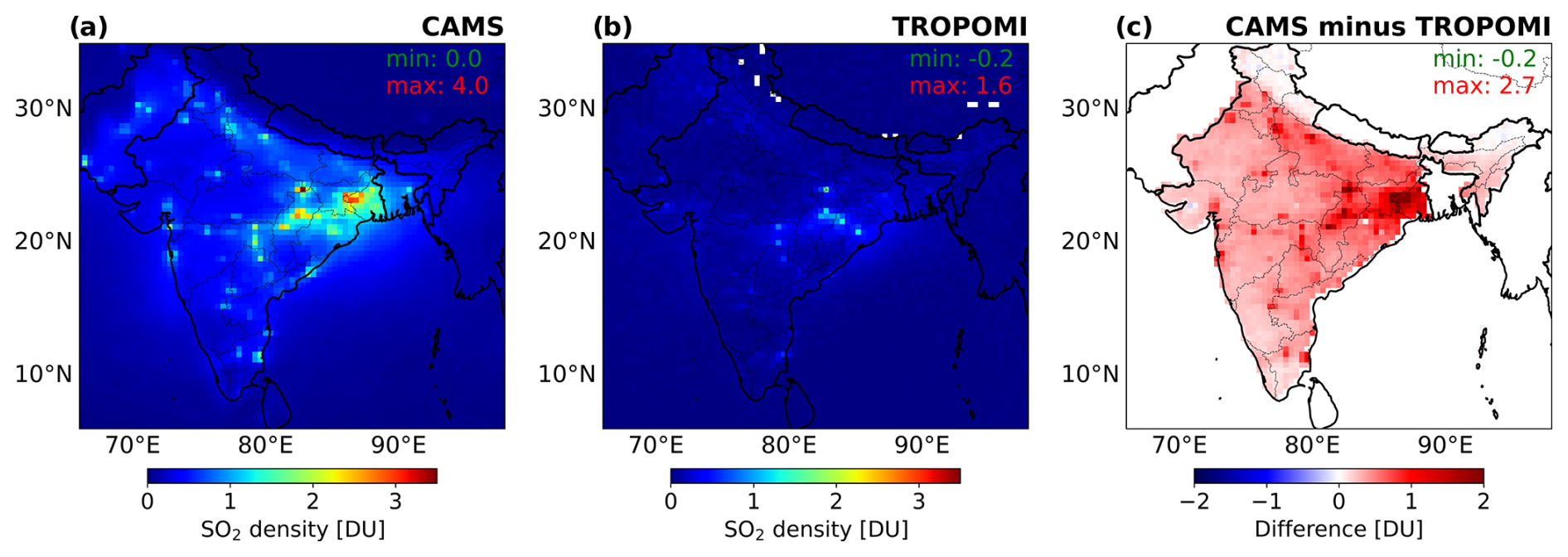
Figure 9 Indian SO₂ vertical column densities (VCDs) averaged in 2023 from (a) the CAMS global composition forecast dataset and (b) the TROPOMI Level-2 COBRA dataset (at about the overpass time of 06:00 UTC). We integrate the TROPOMI observations to a resolution of 0.4° × 0.4°, the same as the CAMS datasets. Panel (c) is the difference obtained by subtracting (b) from (a). The data of the same days are used for comparison. The CAMS SO₂ density with total cloud coverage larger than 30 % is excluded from the averaging.

The total SO₂ emissions in India were similar in 2019 and 2023, with lower emissions in the years in between. To explore the changes in detail, the difference in emissions between 2019 and 2023 of each point source is shown in Fig. 10. Overall, the total point-source emissions are estimated to be 2.8 Tg yr⁻¹ in 2019 and 3.0 Tg yr⁻¹ in 2023. The point sources exhibiting the largest changes belong to our top 10 sources. The emissions of Vindhyachal, the point source showing the largest decrease, were reduced by 17 %, which is about 43 Gg yr⁻¹. This reduction may be partially attributed to the initiation of a carbon capture project at the Vindhyachal plant started in August 2022 (PTI, 2022), which likely mitigates some of the SO₂ emissions (Wang et al., 2011; Corvisier et al., 2013; Gimeno et al., 2017). The largest increasing emitter, Baradarha, increased over 75 %, which is in total 107 Gg yr⁻¹ of SO₂ emissions.

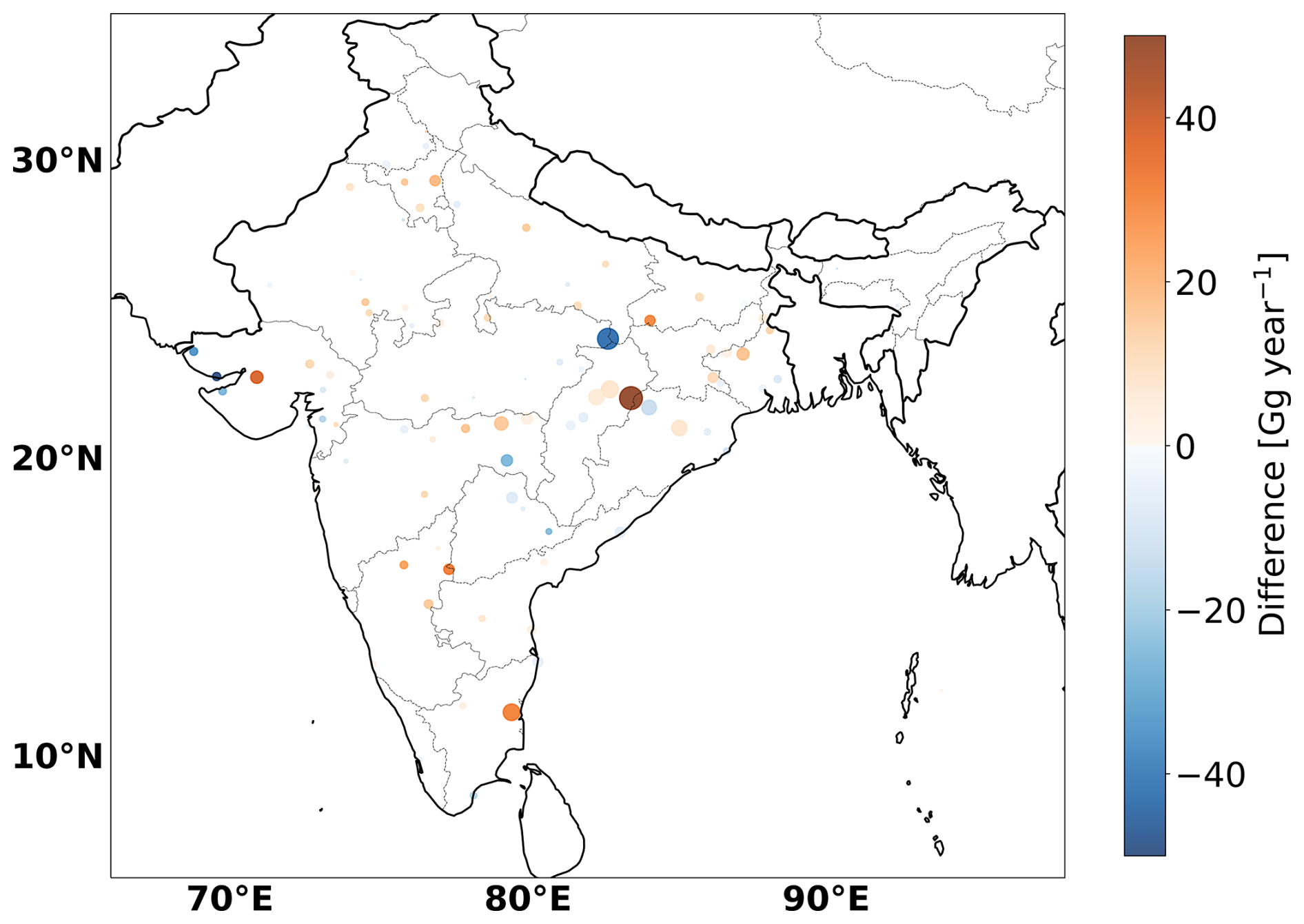
Figure 10 Absolute changes in the derived SO₂ emissions for the most important point sources between December 2018 and November 2023. The circle size denotes the size of the emissions in the last year (December 2022 to November 2023). The circle color means changes in the last year compared to the emissions in the first year (December 2018 to November 2019).

7 Discussion

The hard-to-quantify factors influencing the lifetime and emissions are discussed here. First, our grid-averaged (about 40 km × 40 km) OH climatology may not resolve detailed chemical variation within the pollutant plumes, particularly those involving the interaction between SO₂ and OH. Krol et al. (2024) studied the chemistry within the NO_x plumes and observed low OH concentrations near the strong NO_x sources (within an average of 10 km) and enhanced OH away from the sources. This suggests that our 40 km averaged OH climatology cannot capture this OH decline and may underestimate the SO₂ lifetime near the large NO_x sources. Furthermore, the variation of OH concentration between 10 km to 40 km is roughly limited to 10 %; see Fig. 7b from the study of Krol et al. (2024). We have considered these effects in our error estimate of the lifetime. Second, we did not consider the heterogenous SO₂ reactions on wet aerosols. We suppose this impact on SO₂ lifetime can be neglected in our study. Analysis of the dominant term for conversion in the CAMS system shows aqueous-phase chemistry is the dominant term related to sulfate production rather than heterogeneous reactions. We therefore assume wet aerosols are a negligible source term (which typically have low pH and slow sulfate production; Gillani et al., 1981). Even though the atmospheric SO₂ in the gas phase can convert to the aqueous phase and be oxidized to form sulfate on the wet surface of aerosols or within clouds, these reactions typically occur on hazy days with high relative humidity and PM_2.5 level (Ge et al., 2021). These meteorological conditions are generally not favored on days with minimal cloud coverage, as achieving the necessary high relative humidity is difficult with ample sunlight at noon. Finally, we only calculate the lifetime for SO₂ in cloud-free regions, excluding the SO₂ wet deposition and the reactions within the clouds. This is actually the lifetime we need in our inversion since the TROPOMI observations of SO₂ plumes are limited to cloud-free scenes.

8 Conclusion

In this study, we derived Indian SO₂ emissions using an improved flux-divergence method including a non-constant SO₂ effective lifetime for cloud-free conditions. The improved divergence method largely removes the spreading effect on emissions that is typically introduced by the discretization in calculating the divergence. The non-constant lifetime approach is more representative with respect to season and latitude as compared to adopting a fixed lifetime for the derivation of emission fluxes, especially for short-living species like SO₂. Based on the non-constant lifetime, the improved divergence method further constrains the SO₂ emissions more closely to its source. The SO₂ effective lifetime in India for cloud-free conditions, derived from the SO₂ chemical lifetime and dry deposition lifetime, is calculated for each grid cell. The SO₂ chemical lifetime is primarily derived using an OH monthly climatology (December 2018 to November 2023) from CAMS simulations. The variability in the monthly mean SO₂ effective lifetime varies from 16 to 34 h, with the longer chemical lifetime occurring in the winter season. The seasonality of the SO₂ chemical lifetime is driven by the OH concentration, which is largely influenced by sunlight. Significantly different chemical lifetimes were also noted across various regions within the same season. The chemical lifetime in northern India is generally larger than in the south in spring, winter, and autumn. The SO₂ monthly dry deposition lifetime varies from 55 to 135 h. After accounting for the SO₂ dry deposition, the seasonality and regional variation of lifetime are reduced. The SO₂ effective lifetime is 27 % lower on average compared to the chemical lifetime. The SO₂ monthly mean effective lifetime varies from 12 to 19 h with uncertainties of −20 % to +60 %. Our local effective lifetime calculations align with a recent study, demonstrating that the species lifetime varies spatially due to the spatial variation of the influencing factor (Krol et al., 2024).

Since the data are available on a grid scale instead of a continuous state, the divergence calculation will introduce a spreading effect to the calculated SO₂ divergence and emissions. To reduce the spreading effect, we have tested two divergence allocation methods on the resolution of 0.4° × 0.4°, 0.1° × 0.1°, and TROPOMI-measured pixels and concluded that assigning all flux divergence to the grid cell with the larger SO₂ VCD improved the results. After the implementation of the improved flux-divergence method, the smoothing of the emission map is mitigated efficiently. An emission map with more distinct emission signals has been obtained.

Implementing the improved method with a non-constant SO₂ lifetime, we calculated the SO₂ emissions for India from December 2018 to November 2023. The total annual SO₂ emissions we found for this period is about 5.2 Tg yr⁻¹ with a monthly mean uncertainty of 40 %. The total annual SO₂ emissions decreased from 2019 to 2020 due to the COVID-19 quarantine measures and then gradually increased to the same level as before COVID-19 in 2023. In contrast to the trend from MSAQSO₂LV4 showing that the SO₂ emissions reaching its highest point in 2022, our emissions in 2022 are the same as those in 2021 and lower than the emissions in 2019 and 2023. Even though the total power generation in 2022 is higher than the previous years (https://powermin.gov.in/en/content/power-sector-glance-all-India, last access: 29 July 2024), the comparable emissions between 2021 and 2022 might be a result of the growth of renewable and non-fossil fuel power generation in 2022 (https://powermin.gov.in/en/content/overview, last access: 29 July 2024).

The 92 SO₂ large point sources are compared with the global catalog MSAQSO₂LV4. Our total emissions of 2.9 Tg yr⁻¹ are lower than the total emissions from MSAQSO₂LV4 of 5.2 Tg yr⁻¹. The difference is mainly because Fioletov et al. (2023) used a fixed 6 h lifetime for calculating emissions, while our derived monthly effective lifetimes varied from 12 to 19 h. Using the fixed 6 h lifetime can result in a smoothing of emission map with the divergence method and may lead to overestimation of the emissions. Our results show the SO₂ emissions of the 92 point sources in India are similar between 2019 and 2023. The SO₂ emissions at the largest point source, Vindhyachal, show a reduction in recent years. This might be due to the initiation of a carbon capture project at Vindhyachal.

With the improvement in the divergence method and locally derived variability in the lifetime, gridded SO₂ emissions over a large area can be estimated efficiently. This method can be applied to any region in the world to derive SO₂ emissions with a 0.1° × 0.1° resolution based on TROPOMI observations. For those regions with more northerly latitudes than 40° N (e.g., northern China, eastern Europe), the latitude- and season-dependent SO₂ lifetime with the improved divergence calculation approach has the potential to significantly improve the top-down derivation of SO₂ emission estimates. This paper is considered a first step towards addressing the lifetime variability in the inversion methodology.