Tropical tropospheric ozone trends (1998 to 2023): new perspectives from SHADOZ, IAGOS and OMI/MLS observations

Tropospheric ozone trends are important indicators of climate forcing and surface pollution, yet relevant satellite observations are too uncertain for assessments. The assessment project TOAR-II has used multi-instrument, ground-based data for global trends over 2000–2022 (Van Malderen et al., 2025a, b). For the tropics, trends are derived from SHADOZ ozonesonde profiles (Thompson et al., 2021, “T21”; Stauffer et al., 2024) or combinations of satellite, SHADOZ and IAGOS aircraft measurements (Gaudel et al., 2024). We extend T21 that covered 1998–2019, analyzing SHADOZ data at five sites with a Multiple Linear Regression (MLR) model for 1998–2023 and reporting trends for two free-tropospheric (FT) segments, the lowermost stratosphere and the total tropospheric column (TrCO_sonde). Trends for the Aura period, 2005–2023, are computed from OMI/MLS TrCO_satellite. We find the following:

1. Extending SHADOZ analyses 4 years shows little change from T21; TrCO_sonde trends are small (0.5–1 DU/decade) except over SE Asia.

2. Annual trends for TrCO_sonde and OMI/MLS TrCO_satellite agree within uncertainties at four of five sites, with the largest differences at Samoa. Sensitivity tests show the following:

   •  

     (a) Adding thousands of FT IAGOS profiles to SHADOZ yields little change in trends; SHADOZ sampling is sufficient.

   •  

     (b) Quantile Regression (QR) and MLR median trends are both near zero, but QR captures extremes (5th percentile, 95th percentile) with changes up to ±1 DU/decade (p< 0.10).

   •  

     (c) Twelve-year analyses for trends lead to uncertainty changes too large for an assessment.

3. This study and Van Malderen et al. (2025a, b) provide the most reliable TOAR-II trends to date: over the past ∼ 25 years, tropical FT ozone changes have been modest, ∼ (−3–+3) %/decade, except over SE Asia.

1 Introduction

The importance of tropical tropospheric ozone in atmospheric composition and climate variability has long been known (Lacis et al., 1990; Schwartzkopf and Ramaswamy, 1993). Although the thickness of total column ozone (TrCO) in the tropics (∼ 250–325 Dobson units, DU; 1 DU$=\mathrm{2.69}\times {\mathrm{10}}^{\mathrm{16}}$ cm⁻²) is much less than in the extra-tropics (350–450 DU), the latitude band from −30 to +30° covers roughly one-half of the Earth's surface. In this region tropospheric ozone is a major source of global OH (hydroxyl radical), key to Earth's oxidizing capacity (Thompson, 1992), controlling the lifetimes of countless biogenic and anthropogenic species. Global OH also controls the lifetime of methane, a powerful greenhouse gas with both natural and anthropogenic sources (Khalil, 2000). Methane (CH₄) increases alone add ozone to the troposphere, and methane's oxidation by OH to carbon monoxide (CO), which also affects the amount of OH, establishes a feedback cycle among O₃–OH–CH₄–CO (Thompson and Cicerone, 1986; Thompson et al., 1990). Regional variability in factors controlling the cycle derives from local levels of the shorter-lived nitrogen oxides and reactive volatile organic compounds. The tropics/subtropics (−30 to +30°) is where the “tropical pipe” (Plumb, 1996) carries ozone and ozone-destroying trace species from the tropics into the mid-latitude lowermost stratosphere (LMS).

Trends in tropical tropospheric and LMS ozone are of interest for several reasons. First, free-tropospheric (FT) ozone is an important greenhouse gas. There is a potential for significant changes in FT ozone because parts of the tropics are in areas of rapid changes in emissions. These may be caused by economic development (Zhang et al., 2016) and/or variations in land use and fire activity (Christiansen et al., 2022; Tsivlidou et al., 2023). Second, with relatively low ozone amounts relative to the extra-tropics, ozone near the tropical tropopause is highly sensitive to dynamical interactions (Randel et al. 2007). Analyses of ozone profiles over the past ∼ 25 years have found regional meteorological changes propagating to seasonal ozone increases. Stauffer et al. (2024) verified that a suspected decline in early-year convection (Thompson et al., 2021; hereafter T21) drove 1998–2022 ozone increases over equatorial southeast Asia. New reports on decreasing tropical cloud cover (Tselioudis et al., 2025) and a shift in ITCZ location (Aumann et al., 2024) may indicate changes in convection. At Réunion Island, shifting anticyclones caused an increase in FT ozone from 1998–2023 (Millet et al., 2025). Recurring influences of climate oscillations on FT and LMS ozone are well-documented in ozonesonde and satellite data (Thompson et al., 2001; Ziemke and Chandra, 2003; Ziemke et al., 2006, 2019; Lee et al., 2010; Randel and Thompson, 2011; Thompson et al., 2011).

1.1 The TOAR project and challenges in assessing tropospheric ozone trends

Context for this study comes from the International Global Atmospheric Chemistry/Tropospheric Ozone Assessment Report (IGAC/TOAR) that is completing its second phase, TOAR II, initiated in 2020. The first TOAR, designated here as TOAR I and published as a collection of 11 papers in Elementa, 2017–2020 (https://online.ucpress.edu/elementa/toar, last access: 15 July 2025) included an assessment of surface ozone changes (Chang et al., 2021) based on a vast set of surface ozone measurements from seven continents (Schultz et al., 2017). However, because the FT is the region of greatest radiative forcing by ozone, the trend community needs profile data. Ozone observations for the FT are relatively sparse. A TOAR I evaluation by Tarasick et al. (2019) pointed out the uneven geographic coverage of ozone profiles from soundings (∼ 60 publicly available station records since the early 1990s) and aircraft landing and takeoff profiles to ∼ 250 hPa that are used for FT ozone analyses. Tarasick et al. (2019) also questioned the suitability of all ground-based techniques (sonde, aircraft, lidar, passive spectrometers) for monitoring FT ozone using illustrations from multi-decadal records that include obsolete techniques, evolving versions of instruments and/or inconsistent absolute calibration. Nonetheless, several follow-on studies to TOAR I employed sonde (T21) and commercial aircraft data (from the In-service Aircraft for a Global Observing System, IAGOS; https://www.iagos.org, last access: 15 July 2025), with 5 %–10 % accuracy or better, to estimate trends from the 1990s to ∼ 2018 (Gaudel et al., 2020; Thouret et al., 2022).

Efforts to fill gaps with tropospheric ozone estimates from satellite data, preferred over in situ methods for their even global coverage, have been mixed. For TOAR I, Gaudel et al. (2018) pointed out that trends derived from five satellite products covering the tropics and mid-latitudes for the 2005–2016 period differed from one another, not only in magnitude but also in sign. The newer TOAR II evaluation of six satellite products for 2015–2019 over the tropics (Gaudel et al., 2024), where satellite estimates tend to be most reliable (T21), exhibited a range of values. Not only were uncertainties among the products highly variable; comparisons of monthly mean satellite columns with sonde and IAGOS profiles up to 270 hPa exhibited r² correlations as low as 0.27.

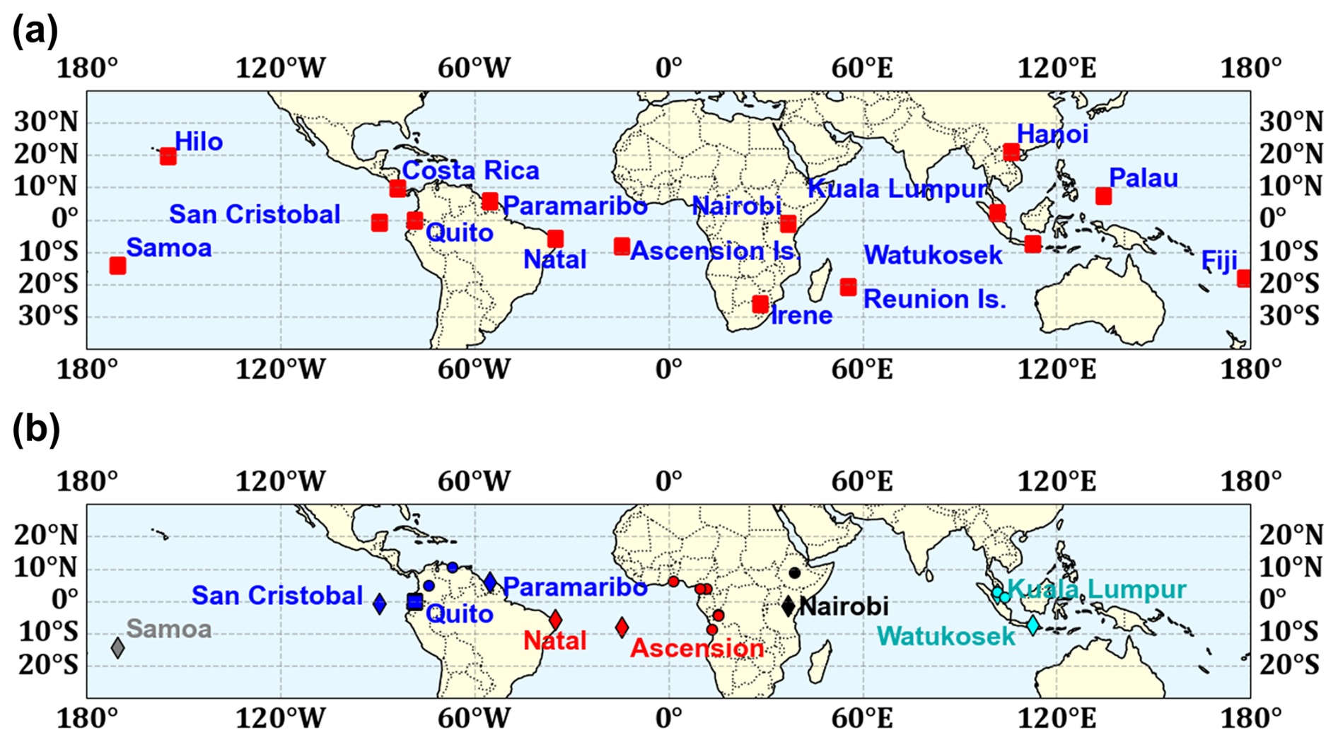
Figure 1 (a) Map of all SHADOZ stations in 2025 when the Quito and Palau records, that began in 2014 and 2016, respectively, joined the network. (b) SHADOZ sites used in T21 for 1998–2019 equatorial trends and here for 1998–2023 trends are represented with diamonds. SHADOZ stations whose combined records are examined within regions are colored blue for Equatorial Americas, red for Atlantic and cyan for equatorial southeast Asia. The airport locations from IAGOS include those indicated with circles: red for Atlantic and West Africa, black for East Africa, and cyan for the equatorial Southeast Asia region. For T21 and the trends here, the fifth station is Samoa (in gray). Quito (blue square) data are included in the Equatorial Americas trends of Table 3. All station and airport locations are in Table 1. The five SHADOZ sites (two individual and three combined) from T21 and for which trends are updated here appear in Table 2 with the MLR trends. Individual SHADOZ and IAGOS site names within each region and their trends are shown in Table 3. Trends computed by QR for total column and FT ozone at 13 individual SHADOZ stations are summarized in Table 4.

Other TOAR II studies also reveal a persistent uncertainty in the application of satellite data for trend analyses. Pope et al. (2023) published global trends from 2005–2017 OMI total column ozone data that are too high because of a drift in OMI that was corrected in Gaudel et al. (2024). The latter study led to a satellite-based estimate for tropical ozone trends for 2005–2019 of ∼ (0.5–3) ppbv/decade for TrCO (tropospheric column ozone), similar to or slightly larger than T21. Trends determined from non-UV satellite instruments have been disappointing (Gaudel et al., 2018). A TOAR II contribution by Froidevaux et al. (2025) examined changes in tropical ozone (± 26° latitude) over the 2005 to 2020 period using measurements from the three lowest levels of MLS (Microwave Limb Sounder). Unfortunately, the zonal structure of MLS data at the 146 and 213 hPa levels (Fig. 1 in Froidevaux et al., 2025) shows that the prominent ozone wave-one feature, associated with the Walker circulation (Thompson et al., 2003, 2017), is absent; i.e., MLS does not capture regional differences as OMI-based products do. Froidevaux et al. (2025; Figs. 1, 2, 5) compare the MLS global structure to ozone output at 215 and 146 hPa from three models, Whole Atmosphere Community Climate Model (WACCM6) and two variants of the Community Atmosphere Model with Chemistry (CAM-Chem), each variant using different anthropogenic emissions. The models are likewise zonally uniform in upper-tropospheric (UT) ozone, so they do not yield meaningful tropical upper-tropospheric ozone trends either.

A TOAR II-related investigation (Boynard et al., 2025) uses IR-based retrievals from the MetOP IASI satellite instrument to determine trends for the period 2008–2023. As in Gaudel et al. (2018) the newer IASI tropospheric ozone climatology differs from that of UV-based products; IASI's negative ozone trends also disagree with increases from UV-based products. Boynard et al. (2025) offer little explanation for the discrepancies. They note that their 12-year period trends (2008–2019), roughly half as long as the sonde or aircraft trends in T21 or Gaudel et al. (2024), may be too short for a statistically robust result. Pennington et al. (2025) does provide some insight into long-term changes of three satellite IR products (TROPESS CrIS, AIRS, AIRS+OMI) compared to ozonesondes. They find that the global tropospheric ozone satellite-sonde bias is approximately one-third of the magnitude of trends in global tropospheric ozone reported by TOAR I.

Keppens et al. (2025) addressed the question of whether satellite data harmonization for nadir ozone profile and column products improves satellite data consistency for both their mean distributions and long-term changes. They concluded that their harmonization methods reduce inter-product dispersion by about 10 % when comparing to global ozonesonde datasets from 43 sites, but there is a significant meridional dependence, and the dispersion reduction is not consistent in space or time. This implies that a substantial part of the inter-product differences is instrument- and/or retrieval-specific and that the harmonization methods have limited application to TOAR II. An alternate method of combining the residual and profile products with a column fill-in method is expected to be published as the TOAR II “satellite assessment.”

1.2 TOAR II studies with ground-based measurements and statistical issues

TOAR II has engaged a more globally representative set of researchers than TOAR I and reports data and analyses from a larger set of observations. Dozens of TOAR II-related publications can be reviewed at https://bg.copernicus.org/articles/special_issue10_1256.html (last access: 15 July 2025). Given the persistent uncertainty of the satellite records, a number of TOAR II contributors formed a community project, the Harmonization and Evaluation of Ground-based Instruments for Free-Tropospheric Ozone Measurements (HEGIFTOM), to apply newly standardized ozone measurement and processing protocols for data from sondes, aircraft and other ground-based (GB) instruments: FTIR, tropospheric ozone lidar and Umkehr retrievals from Dobson spectrometers. The rationale is that GB networks, with stable operations at fixed sites and well-calibrated instruments, e.g., as in the Network for Detection of Atmospheric Composition Change (NDACC; De Mazière et al., 2018), provide suitable time series at dozens of sites over seven continents and pole to pole. HEGIFTOM has two objectives: (1) harmonizing data from ∼ 80 long-term stations (1990s to 2023) in four GB networks using the most up-to-date reprocessing techniques with each record referenced to absolute standards and (2) calculating trends for the 2000 to 2022 period with harmonized data, reporting station trends with uncertainty. The trends for 55 individual stations are tabulated and illustrated in Van Malderen et al. (2025a; referred hereafter to as HEGIFTOM-1). Regional trends based on merging selected stations in densely sampled areas appear in Van Malderen et al. (2025b; referred hereafter to as HEGIFTOM-2).

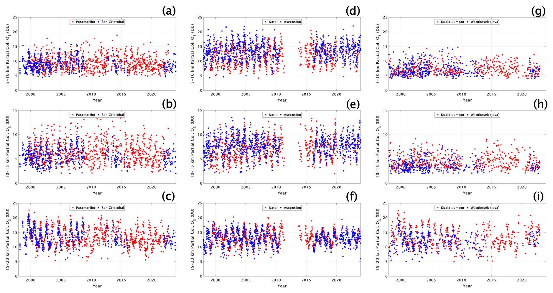
Figure 2 Time series of ozone column segments (in DU) for the combined SHADOZ stations, for the layers 5–10, 10–15 and 15–20 km for San Cristóbal–Paramaribo (a–c), Natal–Ascension (d–f) and Kuala Lumpur–Watukosek (Java) (g–i). Station coordinates in Table 1.

Early in the TOAR II study period we analyzed ozone profiles in the tropics collected in the Southern Hemisphere Additional Ozonesondes (SHADOZ) network (Thompson et al., 2003, 2017) to compute FT and LMS ozone trends. The results in T21 are based on data from eight combined SHADOZ stations within ± 15° latitude; the Goddard Multiple-Linear Regression (MLR) model calculated trends from 1998 through 2019 from the surface to 20 km. Changes in individual layers between 5 and 15 km were typically (5–10) %/decade but only seasonally; over the equatorial SE Asian stations at Kuala Lumpur and Watukosek, Indonesia, some layers displayed increases up to 20 %/decade (Fig. 6 in T21). However, in general, annually averaged changes in equatorial regions ranged from ∼ 0 to +(1–2) %/decade or −(1–2) %/decade. In T21 LMS ozone (LMS defined as within 15–20 km) computed with the MLR model displayed a seasonal loss up to 10 %/decade (July through September) or to 3 %/decade, annually averaged. The loss maximized at ∼ 18 km. At the same time of year, a positive trend in tropopause height (TH), derived from the SHADOZ radiosondes, was detected. Redetermining LMS ozone changes in the 5 km column above the tropopause zeroed out the apparent trend.

More recently, the Stauffer et al. (2024, referred to as S24) paper demonstrated that over the 25-year period 1998–2022, early-year (February through April/May) FT ozone increases in SHADOZ data are associated with declining convection, most pronounced over SE Asia but observed to a lesser degree at the other stations. With the newest OMI/MLS-based satellite estimates of total tropospheric column ozone (TrCO), Gaudel et al. (2024) showed that over the Aura era (2005–2019) trends from satellite, SHADOZ and IAGOS aircraft profiles were in good agreement with one another over southeast (SE) Asia, similar to S24. SHADOZ only (T21) and IAGOS trends (Gaudel et al., 2024) diverge somewhat over the Equatorial Americas and Africa, partly due to a difference in sampling sites, e.g., West African IAGOS profiles in Gaudel et al. (2024) vs the SHADOZ Nairobi station.

1.3 This study

We use the Goddard MLR model to calculate trends in monthly mean SHADOZ data for the period 1998 through 2023, addressing the following questions:

• Compared to T21, that reported on the 1998–2019 period, what do FT and LMS ozone trends look like in the equatorial zone (−15 to +15°) with 4 additional years of SHADOZ profiles? Because the extension covers 2020 to 2023, the comparisons are looking for impacts of COVID-19 (Steinbrecht et al., 2021; Ziemke et al., 2022).

• How do trends in tropospheric ozone for 1998–2023 compare to trends for 2000 to 2023? In other words, is the 26-year trend biased by SHADOZ starting at the end of the 1997–1998 El Niño–Southern Oscillation (ENSO) that produced strong perturbations to tropical ozone (Thompson et al., 2001)?

• How do SHADOZ total tropospheric column changes (TrCO_sonde) compare to OMI/MLS column ozone trends over the 2005–2023 period? Do the satellite data capture the seasonality of sonde-derived trends as noted in T21 and S24?

In addition to updated trends for equatorial SHADOZ sites, we have used SHADOZ profiles to investigate three statistical issues raised in HEGIFTOM-1 and other TOAR II studies.

• HEGIFTOM-1 calculated median trends for sondes and all other GB data using both Quantile Regression (QR) and MLR models. Within the associated uncertainties of each, the two methods gave identical results for annually averaged trends. Here we explore special features of QR and MLR to learn more about the nature of the trends, e.g., seasonality (MLR) and changes in the highest and lowest quantile (QR).

• Second, we use MLR to evaluate the sensitivity of trends on sample size as raised in TOAR II papers (Chang et al., 2020, 2021; Gaudel et al., 2024) and HEGIFTOM-1 by augmenting equatorial SHADOZ data with tropical IAGOS profiles for the appropriate region. These calculations are carried out for FT ozone, i.e., in the region where radiative forcing is most effective and both sondes and aircraft sample (700–300 hPa, roughly 5–10 km).

• Satellite records are variable in length, with the most frequently used tropospheric estimates starting after 2004 and a number of products merging measurements from multiple instruments. We examine the sensitivity of trends to length of the observation period using QR by comparing the 26-year SHADOZ ozone trend to a recalculation that coincides with the IASI period 2008–2019 for which trends are reported in Boynard et al. (2025).

Data and analysis methods appear in Sect. 2 with “Results and discussion” in Sect. 3. Section 4 presents “Summary and conclusions”.

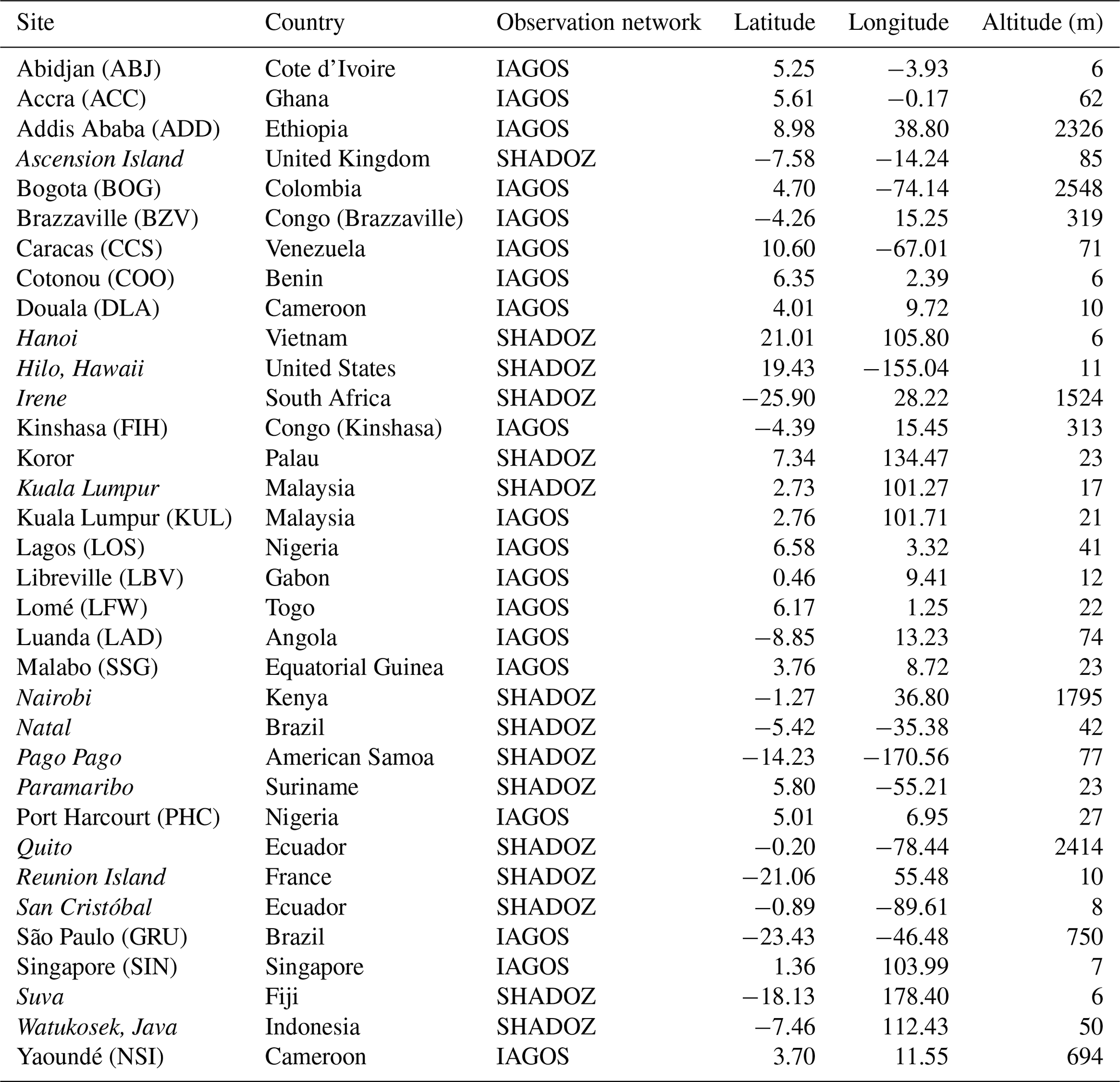
Table 1 List of the 27 total SHADOZ (italicized) and IAGOS sites, and their metadata, used in this analysis.

2 Data and methods of analysis

2.1 Ozone datasets

Three datasets are used in our study: ozonesonde profiles from the SHADOZ network, partial ozone profiles from the IAGOS commercial aircraft network and monthly averaged OMI/MLS tropospheric ozone column estimates from 2005 through 2023.

2.1.1 SHADOZ ozonesonde observations

Figure 1a displays the SHADOZ network stations, italicized with coordinates in Table 1. Quito (Cazorla, 2016; Cazorla et al., 2021; Cazorla and Herrera, 2022) and Palau (Müller et al., 2024) soundings, taken since 2014 and 2016, have recently been added to the archive at https://tropo.gsfc.nasa.gov/shadoz (last access: 3 September 2025). The ozone profiles are obtained from electrochemical concentration cell ozonesondes coupled to standard radiosondes as described in earlier publications, e.g., Thompson et al. (2003, 2007, 2019). The profiles are archived with ozone uncertainties calculated with each individual ozone partial pressure available as separate files in the SHADOZ archive (Witte et al., 2018; WMO/GAW Rep. 268, 2021). Recent evaluations of ozonesonde data have established the quality of the global ECC network. Measurements of total column ozone (TCO) from 60 global ozonesonde stations have averaged within ± 2 % agreement with total ozone from four UV-type satellites since 2005 (Stauffer et al., 2022). About half the SHADOZ stations exhibit a ∼ 3 %–5 % dropoff in stratospheric ozone (Stauffer et al., 2020) that is not completely understood (Nakano and Morofuji, 2023; Smit et al., 2024). Accordingly, our study only uses ozone data below ∼ 50 hPa, defining the range of the lowermost stratospheric (LMS) ozone as bounded by 15–20 km.

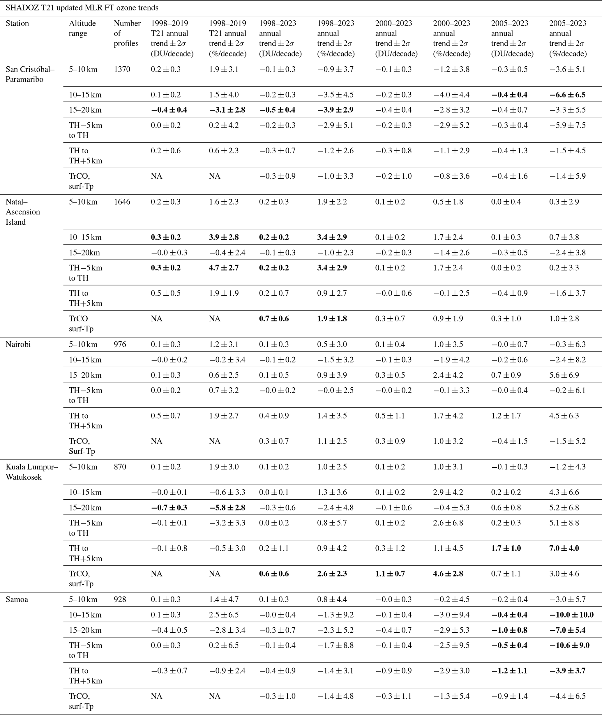
Table 2 SHADOZ metadata: number of profiles and annual trends. Each row indicates a different segment: 5–10, 10–15, 15–20 km, TH−5 km to TH, TH to TH+5 km and surface to Tp (tropopause). Periods analyzed (columns) are 1998–2019 (T21), 1998–2023, 2000–2023 and 2005–2023 for OMI/MLR comparisons in total tropospheric ozone column amount (TrCO). Annually averaged MLR partial column ozone linear trends are shown in DU per decade and in percent per decade, with the 95 % confidence interval. Trends with p values <0.05 are shown in bold.

For the update to T21, that was based on 1998–2019 SHADOZ V06 ozonesonde data (https://doi.org/10.57721/SHADOZ-V06, NASA Goddard Space Flight Center (GSFC) SHADOZ Team, 2019), the same records for eight equatorial sites, located between 5.8° N and 14° S (color-coded in Fig. 1b; italicized in Table 1), are used with 4 additional years (2020–2023) of ozone and P–T–U (pressure–temperature–humidity) profiles. These eight stations have at least 14 years of data between 1998 and 2023, although several have multi-year gaps (Figs. 2, 3 and Fig. S1 in the Supplement). For more reliable statistics three of the “stations” or “sites”, as they are referred to (Fig. 1b), are defined by combining profiles from pairs of launch locations abbreviated as follows: SC-Para for San Cristóbal–Paramaribo (dark blue dots in Fig. 1b); Nat-Asc for Natal–Ascension (red dots in Fig. 1b); KL-Java (cyan dots in Fig. 1b) for Kuala Lumpur–Watukosek (Table 2). T21 (see Supplement) describes multiple tests that were conducted to verify that these combinations are statistically justified. Annual cycles in absolute column amounts (Fig. 2) and anomalies for the pairs were well-correlated. In T21 (Supplement) total tropospheric columns integrated from sondes (TrCO_sonde) at the eight individual stations were also well-correlated (r²=0.72) with colocated TrCO_satellite from OMI/MLS data over the period 2005–2019. It is important to note that the eight well-correlated sites are within 15° latitude of the Equator. The correlation falls to r²=0.50 when comparisons are made between sondes and satellite columns for the four subtropical SHADOZ stations. FT ozone at those locations includes seasonally dependent mixtures of tropical and extra-tropical air masses, with latitudes (Table 4) spanning Hanoi (+21.0) to Irene (−25.9).

Table 3 SHADOZ and IAGOS combined MLR ozone trend values for FTp (700–300 hPa) partial column for five regions: Equatorial Americas, Atlantic and West Africa, East Africa, Equatorial Southeast Asia, and Samoa (individual record). The individual sites are listed for each region. Annually averaged MLR partial column ozone linear trends are shown in DU per decade and in percent per decade, with the 95 % confidence interval. Trends with p values <0.05 are shown in bold.

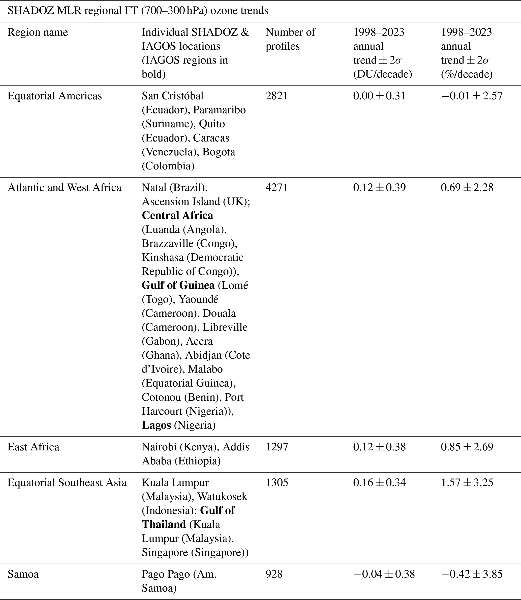
Table 4 SHADOZ QR median (50th percentile) annual ozone trend values (1998–2023) for TrCO (surface to tropopause) and FTp (700–300 hPa) columns in DU/decade and in %/decade with ± 2σ. Trends with p values <0.05 are shown in bold. L1 data are daily data from the HEGIFTOM database (https://hegiftom.meteo.be/datasets, last access: 15 July 2025). The italicized stations are the subtropical SHADOZ stations, defined as latitude outside of ± 19°.

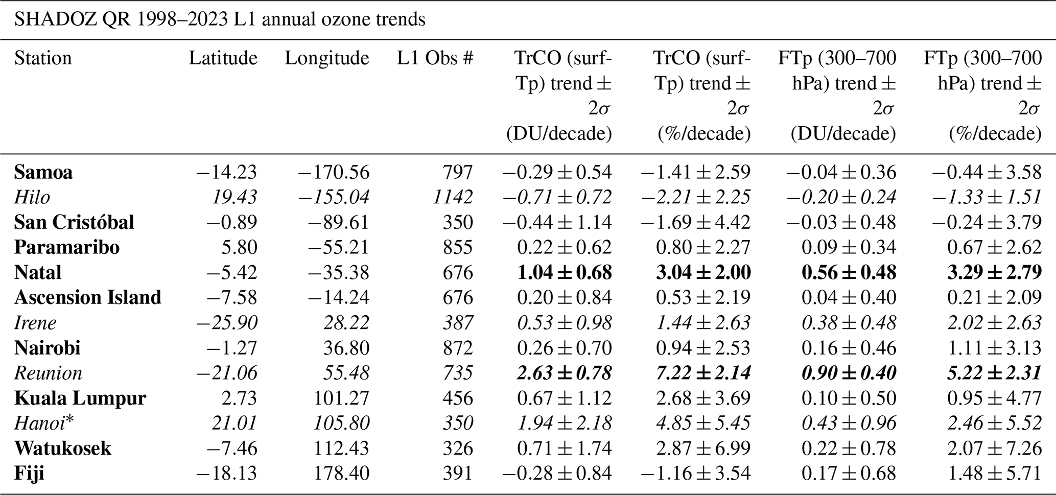
^* Hanoi dataset starts in 2004 (not 1998).

We have also analyzed trends of tropospheric ozone column and free-tropospheric ozone at individual SHADOZ stations using a QR model, following column definitions and guidelines for the TOAR II/HEGIFTOM project analysis (Chang et al., 2023). The tropospheric ozone column in HEGIFTOM trend analysis is defined as the surface to 300 hPa, the FT is defined as a layer between 300 and 700 hPa, and the results are given as ppbv O₃/decade change and %/decade. The QR trends for 13 SHADOZ sites from 2000 to 2022 are summarized in Table 4; a subset of them appear in an evaluation of ground-based global ozone trends in HEGIFTOM-1.

2.1.2 SHADOZ and IAGOS-SHADOZ blended profiles: LMS and FT ozone

The MLR trend analyses (results in Tables 2 and 3) use SHADOZ profile measurements in several ways. First, the trends are computed using monthly averaged ozone mixing ratios at 100 m intervals from the surface to 20 km, as described in T21. Second, most results are illustrated as ozone column amounts (in DU) for two FT segments, 5–10 and 10–15 km, and for the LMS. Trends for ozone and P–T–U data below 5 km are determined for completeness but are not tabulated because station sampling times and local pollution can vary, giving artifact biases among the individual sites (Thompson et al., 2014). We use 15–20 km for the LMS for two reasons. This is where several studies identified wave activity associated with convection and ENSO–La Niña oscillations (Lee at al., 2010; Thompson et al., 2011; Randel and Thompson, 2011; T21). Second, Randel et al. (2007) identified a distinct ozone annual cycle in the 15–20 km range driven by the Brewer–Dobson circulation.

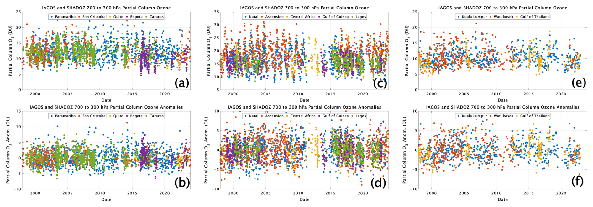
Figure 3 Time series of SHADOZ and IAGOS partial ozone column amounts and partial ozone column anomalies (in DU) for the pressure-defined mid-free troposphere, FTp (700 to 300 hPa), for (a–b) Equatorial Americas, (c–d) Atlantic and West Africa, and (e–f) Equatorial SE Asia. The listing of the individual sites included in these datasets appears in Table 3. Coordinates are in Table 1.

A third way of using SHADOZ profiles in the MLR analysis is in a blend with IAGOS aircraft profile measurements within a lower FT pressure-defined region (“FTp” =300–700 hPa, HEGIFTOM-1). Calculations in the FTp segment are designed to add more samples within the SHADOZ-labeled combination sites (compare profile numbers in Tables 2 and 3) and to augment regional trends in HEGIFTOM-2 where no results are reported for the Equatorial Americas, Atlantic Ocean or most of the African continent. In defining regions for merging SHADOZ and IAGOS observations, we follow locations presented by Tsivlidou et al. (2023). Profiles from the SHADOZ Quito station (2014–2023) and two IAGOS airports (Bogotá and Caracas) are added to the SHADOZ SC-Para profiles to define the Equatorial Americas for determining trends within the FTp (Table 3). Also, for the SHADOZ-IAGOS calculations, sonde profiles from the Natal–Ascension pair are combined with 13 airports in West Africa (Table 3) to determine trends for a region designated “Atlantic+West Africa,” as shown in Fig. 1b (color-coded circles) and the second column of Table 3. In “East Africa” Nairobi sonde data are combined with IAGOS Nairobi and Addis Ababa ozone profiles. The FTp-designated Equatorial SE Asia consists of KL-Java profiles from SHADOZ combined with IAGOS landing and takeoff data from Kuala Lumpur and Singapore. Time series of ozone column amounts (in DU and as anomalies) for SHADOZ stations and airports for these four “regional” sites appear in Fig. 3. The coordinates of individual SHADOZ stations used in the blended dataset (italicized) with IAGOS airports appear in Table 1. Calculations with FTp retain Samoa as a single station.

2.1.3 OMI/MLS satellite and sonde total ozone columns

Trends computed with MLR for sonde-derived total tropospheric ozone columns (TrCO) are based on integrating ozone mixing ratios from the surface to the thermal lapse-rate tropopause derived from the radiosondes that accompany each ozonesonde launch. The standard WMO definition of tropopause is used. For the five equatorial sites in our analyses, the tropopause is typically between 16 and 17 km. Our TrCO_sonde columns and trends are compared to TrCO_satellite, the tropospheric ozone columns estimated from the OMI/MLS residual as described by Ziemke et al. (2019; updated in the TOAR II paper by Gaudel et al., 2024). These newest OMI/MLR TrCO estimates have been corrected for a ∼ 1 %/decade upward drift in OMI over the past 2 decades (Gaudel et al., 2024; Supplement). The OMI/MLS column ozone product is available starting in October 2004. We use monthly average TrCO for both sondes and OMI/MLS between January 2005 and December 2023 (Fig. S1). These are identical to the data used in the Gaudel et al. (2024) TOAR II analyses of tropical ozone.

2.2 Trend analyses

2.2.1 Multiple Linear Regression (MLR) model

As in T21 and S24, the Goddard MLR model (original version Stolarski et al., 1991, updated in Ziemke et al., 2019) is used for analysis of monthly mean ozone amounts. The MLR model includes terms for annual and semi-annual cycles and oscillations prevalent in the tropics: QBO, MEI (Multivariate ENSO Index, v2) and IOD DMI (Indian Ocean Dipole Moment Index; only for KL-Java):

$$\begin{array}{rl}{\mathrm{O}}_{\mathrm{3}}\left(t\right)& =A\left(t\right)+B\left(t\right)+C\left(t\right)\mathrm{MEI}\left(t\right)+D\left(t\right)\mathrm{QBO}\mathrm{1}\left(t\right)\\ & +E\left(t\right)\mathrm{QBO}\mathrm{2}\left(t\right)+F\left(t\right)\mathrm{IOD}\left(t\right)+\mathit{\epsilon }\left(t\right),\end{array}$$

where t is month. The coefficients are as follows: A through F include a constant and periodic components with 12-, 6-, 4-, and 3-month cycles, where A represents the mean monthly seasonal cycle and B represents the month-dependent linear trend. When annual trends are reported, the B term includes only the 12-month component to generate a single trend value over the period of computation. The model includes data from the MEIv2 (https://www.esrl.noaa.gov/psd/enso/mei/, last access: 15 July 2025), the two leading QBO empirical orthogonal functions (EOFs) from Singapore monthly mean zonal radiosonde winds at 10, 15, 20, 30, 40, 50 and 70 hPa levels, and IOD DMI (https://psl.noaa.gov/gcos_wgsp/Timeseries/Data/dmi.had.long.data, last access: 15 July 2025). The ε(t) is the residual, i.e., the difference between the best-fit model and the raw data. T21 noted that the monthly ozone data and MLR model fits for the mid FT (5–10 km) and LMS layers are well-correlated. For the LMS, for example, the correlation coefficients are r=0.83–0.90 (Fig. S7 in T21). The IOD DMI term is included for KL-Java, the only station where the IOD impact on the ozone trend is reliably detected.

The 95 % confidence intervals and p values for each term in the MLR model as presented here are determined using a moving-block bootstrap technique (10 000 resamples) in order to account for auto-correlation in the ozone time series (Wilks, 1997). The model is applied to ozone anomalies in all cases in order to minimize biases that might arise from intersite ozone differences between pairs for the combined stations: SC-Para, Nat-Asc, KL-Java (Table 2). In other words, we calculate ozone anomalies from the individual station's monthly climatology for all profiles before combining the pairs into monthly means and computing the MLR ozone trends. Anomalies are also analyzed for the Nairobi and Samoa station data, although this would be no different than computing MLR trends on the actual ozone time series themselves. The MLR model was separately applied to the monthly mean ozone profile anomalies at 100 m resolution, and the monthly mean partial column ozone anomaly amounts from 5–10, 10–15 and 15–20 km. The MLR model was also applied to the monthly mean tropopause height (TH) anomaly at each station, defined as the 380 K potential temperature surface (e.g., Wargan et al., 2018). Because TH and LMS ozone trends turn out to be strongly correlated (T21), the MLR analysis was also performed for the ozone column amount anomalies referenced to the tropopause. In that case, LMS ozone trends refer to changes in the 5 km above the tropopause with the FT extending from the tropopause to 5 km below the tropopause (Sect. 3, Table 2). Finally, the MLR model was applied to total tropospheric column amounts from the sondes (TrCO_sonde) and corresponding TrCO_satellite from OMI/MLS (surface to Tp in Table 2).

Note that recent ozone trend studies and the TOAR II guidelines (Chang et al., 2020, 2023; Cooper et al., 2020) have discouraged the use of nomenclature associated with statistical significance, whereas the figures and tables presented here refer to trends using terminology of 95 % confidence intervals (equivalent to p value <0.05); the most reliable results in Sect. 3 (bold in Tables 2, 3 and 4) are explicitly stated as based on p values <0.05.

Several studies of tropospheric ozone observations have noted a persistence of COVID-19 perturbations on ozone trends after 2019 (Ziemke et al., 2022; HEGIFTOM-1; HEGIFTOM-2). A comparison of the extended SHADOZ mean ozone trends (1998–2023) relative to those from T21 (covering 1998 to 2019), both summarized in Table 2, represents the impact of COVID-19 in the deep tropics. Likewise, SHADOZ was initiated at the end of the powerful 1997–1998 ENSO. Accordingly, we applied MLR to the same five sites for 2000–2023 to evaluate any artifacts relative to the 1998 to 2023 trends. Those results also appear in Table 2.

2.3 Quantile Regression (QR) model

Whereas MLR has been the standard tool for analyzing global total and stratospheric ozone trends, the latter often with satellite data where zonal means can be used, the TOAR II project has recommended using QR as better suited for ozone trends in the troposphere where, for example, urban concentrations can vary by factors of 3–4. Because it is a percentile-based method (Koenker, 2005), the heterogeneously distributed changes of trends can be estimated, as shown, for example, in Gaudel et al. (2020). To date, the TOAR II HEGIFTOM trend studies for observations at individual sites (HEGIFTOM-1) and regionally organized data (HEGIFTOM-2) have been studied with the QR approach. In those studies and for the 13 individual SHADOZ time series (Table 4), QR has been applied to the median change of the trends, which is equivalent to the least absolute deviation estimator (i.e., aiming to minimize mean absolute deviation for residuals; Chang et al., 2021). The rationale is that compared to least-squares criterion, a median-based approach is more robust when extreme values or outliers are present. Median trends are estimated based on the following multivariate linear model:

$$\begin{array}{}\text{(1)}& \begin{array}{rl}\mathrm{observations}\left[t\right]& =a\mathrm{0}+a\mathrm{1}\times \sin (\mathrm{month}\times \mathrm{2}\mathit{\pi }/\mathrm{12})\\ & +a\mathrm{2}\times \cos (\mathrm{month}\times \mathrm{2}\mathit{\pi }/\mathrm{12})+a\mathrm{3}\\ & \times \sin (\mathrm{month}\times \mathrm{2}\mathit{\pi }/\mathrm{6})+a\mathrm{4}\\ & \times \cos (\mathrm{month}\times \mathrm{2}\mathit{\pi }/\mathrm{6})+b\times t+c\\ & \times \mathrm{ENSO}\left[t\right]+N\left[t\right],\end{array}\end{array}$$

where harmonic functions are used to represent the seasonality, a0 is the intercept, b is the trend value, c is the regression coefficient for ENSO and N[t] represents the residuals. Autocorrelation is accounted for using the moving block bootstrap algorithm, and the implementation details are provided in the TOAR statistical guidelines (Chang et al., 2023). In the individual site analyses of HEGIFTOM observations (HEGIFTOM-1), where all individual ozone records (designated as L1) and monthly means (denoted as L3) were analyzed, annually averaged trends turned out to be the same within uncertainties. Where QR is applied in the present study, L1 ozone data are used.

2.3.1 Trend sensitivity studies

Three sensitivity studies were conducted, related to (1) the sampling frequency, (2) the complementarity of MLR and QR methods, and (3) the duration of time series.

A number of TOAR-related studies (Chang et al., 2020, 2021, 2023) have emphasized links between ozone time series sampling characteristics, i.e., frequency of profile measurements and/or temporal gaps, and trend uncertainty. Gaudel et al. (2024), for example, show uncertainty (as 2-sigma) in median tropospheric ozone profiles; the inference is that 6–15 monthly samples are required for meaningful FT trends (Figs. 1–2 in Supplement, Gaudel et al., 2024). For the first sensitivity test we examined trend dependence on sample size by comparing the annual trends computed with MLR for the lower–mid-FT ozone segment (5–10 km) to the trends from the combined SHADOZ-IAGOS merged monthly mean SHADOZ profiles (L3, 700–300 hPa) for 1998–2023. A comparison of Tables 2 and 3 indicate that for the Equatorial Americas and Atlantic regions, the sample numbers are increased more than a factor of 2; the other two sites have enhancements of 1.3 and 1.5. The results in DU/decade and %/decade appear in Table 3.

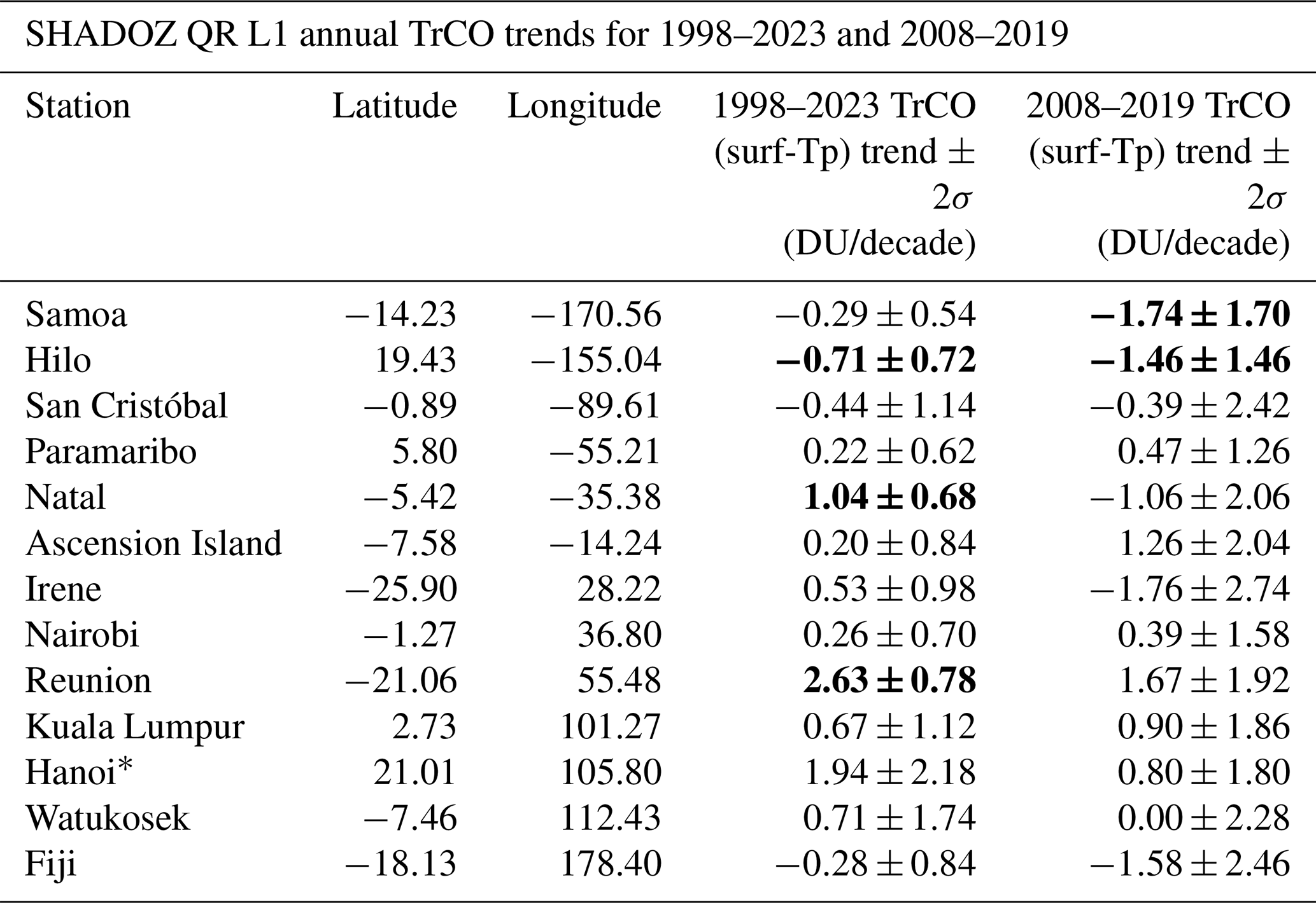
Table 5 SHADOZ QR median (50th percentile) annual ozone trend values (1998–2023 and 2008–2019) for TrCO (surface to tropopause) columns in DU/decade with  ± 2σ. Trends with p values <0.05 are shown in bold. L1 data are daily data from the HEGIFTOM database (https://hegiftom.meteo.be/datasets, last access: 15 July 2025).

^* Hanoi dataset starts in 2004 (not 1998).

In the second sensitivity study three calculations were made using the data from all individual SHADOZ stations as in HEGIFTOM-1, not only the five-site equatorial profiles (Table 2). The individual station results appear in Table 4. The trend (1998–2023) in mean tropospheric column, TrCO (in DU/decade), was computed using the QR method applied to all profiles at each station (L1, level 1 data) with median (50th percentile) trends shown. The L1 sample numbers ranged from 326 (Watukosek) to 1142 (Hilo); the L1/L3 sample size ratios ranged from 2.2 to 4.3, with only 3 of 13 stations having a ratio below 3.2 (i.e., fewer than three profiles per month). These trends can be compared to the MLR trends in Table 2. The second calculation was a computation of trends at each station for the FTp column amount used in HEGIFTOM-1 (700–300 hPa, comparable to our 5–10 km segment in Table 2 and the combined IAGOS+SHADOZ FTp columns in Table 3). HEGIFTOM-1 pointed out the complementarity of applying both MLR and QR to the 23-year time series of mean ozone column amounts. The advantage of MLR is a graphical display of monthly trends that indicate important ways ozone interacts with seasonally varying dynamics, as in S24 or Millet et al. (2025). QR distinguishes trends among different segments of the distribution, an advantage for stations where tropospheric ozone segments are highly variable. To demonstrate this, the QR method (including trends for the 5th percentile, 25th percentile, 75th percentile, 95th percentiles) was applied to IAGOS+SHADOZ combined FT dataset for the four regions: Equatorial Americas, Atlantic+West Africa, East Africa and equatorial southeast Asia.

The third sensitivity test investigates the degree to which trends and uncertainties depend on the length of sampling. This issue arises because the most frequently used satellite estimates of tropospheric ozone begin after 2003 compared to SHADOZ (1998–) and IAGOS (1994–). The Boynard et al. (2025) study uses IASI products for 2008–2019 (and 2008–2023), comparing only 7 of ∼ 40 potential ozonesonde stations for evaluation. Using L1 mean TrCO tropospheric columns, the QR method was applied to the 13 SHADOZ stations for a 12-year period (2008–2019) for comparison. The results in Table 5 demonstrate the impact of sampling in a shortened time series.

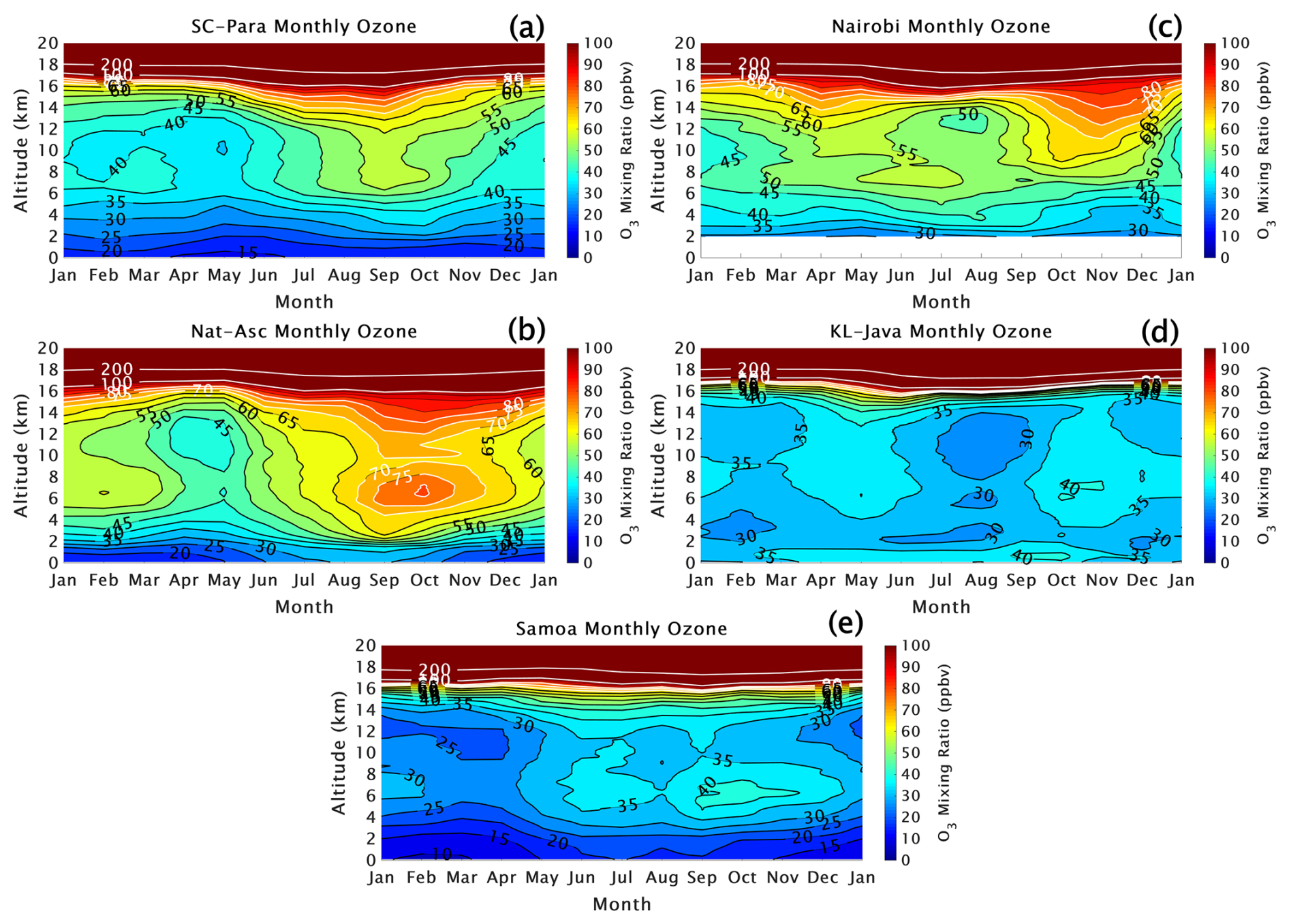
Figure 4 Monthly averaged ozone mixing ratios from the surface to 20 km altitude for the five SHADOZ sites: (a) San Cristóbal–Paramaribo, (b) Natal–Ascension Island, (c) Nairobi, (d) Kuala Lumpur–Watukosek (Java) and (e) Samoa. Colors with black and white contour lines are shown for the ozone mixing ratios in ppbv.

3 Results and discussion

3.1 Monthly and seasonal ozone climatology at five SHADOZ sites

Figure 4 displays the five-site monthly ozone climatology based on SHADOZ monthly averaged data from the surface to 20 km. Regional differences in vertical structure within the FT are pronounced. For example, the contours representing the 60–90 ppbv range (yellow to red colors) are absent in mid-FT ozone over KL-Java or Samoa (Figs. 4d,e). Conversely, FT ozone values ≤30 ppbv (darkest blue shades) observed over KL-Java and Samoa in the middle FT never appear over the other three stations: Equatorial Americas (SC-Para, Fig. 4a), Nat-Asc or Nairobi (Fig. 4b, c). These contrasts may reflect regional differences in ascending vs. descending nodes of the Walker circulation. The latter feature is partly responsible for the tropospheric zonal wave one (Thompson et al., 2003) that refers to a mean TrCO over the south tropical Atlantic Ocean that is sometimes twice as large as over the western Pacific. There is less regional variability in LMS ozone. At all stations (Fig. 4) above ∼ 16 km, the colors and contours are nearly uniform over the year. Mixing ratio contours of 100 and 200 ppbv may appear as a thick white line. The 100 ppbv level is sometimes referred to as an ozonopause; typically it is within 1–2 km of the thermal lapse-rate tropopause.

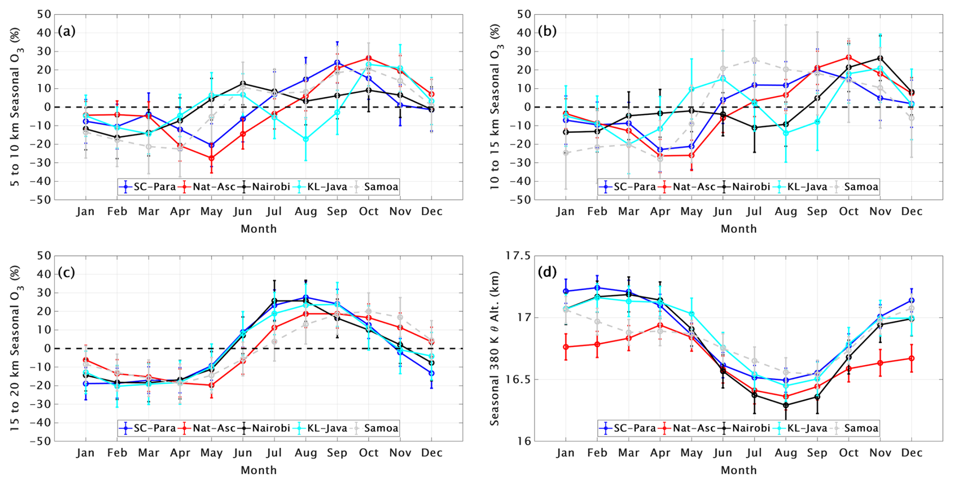
Figure 5 Monthly ozone variability for the five T21 SHADOZ profiles, expressed as percent anomaly from annual mean, determined from the MLR model in the lower and middle FT (5–10 km: a, 10–15 km: b) and for the LMS (15–20 km:  c). The tropopause height (TH) seasonal cycle (d, in km) is based on the 380 K potential temperature surface from the radiosondes. Dots indicate monthly values; error bars display the 95 % confidence intervals.

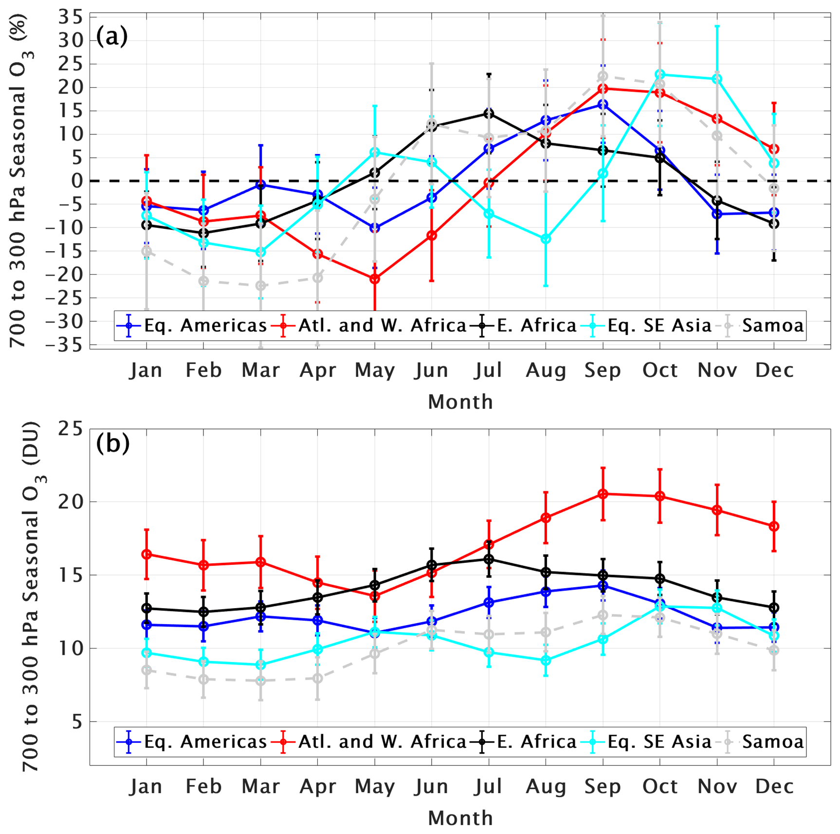
Figure 6 Monthly ozone variability for the five combined SHADOZ+IAGOS regions (defined in Fig. 1 and Table 3), expressed as anomaly from annual mean in (a) percent with actual values in DU (b), for the FTp (700–300 hPa) column. Dots indicate the monthly values; error bars display the 95 % confidence intervals.

3.2 FT and LMS ozone annual cycle (1998–2023)

The annual cycle of ozone at the two FT layers and for LMS ozone appear as anomalies in Fig. 5. FT ozone seasonality (Figs. 5a, b) is less uniform than for LMS ozone (Fig. 5c) and tropopause height (TH, Fig. 5d). Randel et al. (2007) showed that the near-uniform LMS ozone seasonality in the equatorial zone is due to the Brewer–Dobson circulation. The more varied FT ozone cycles in Fig. 5a and b are due to a range of different dynamical and chemical influences across the stations. As expected, the annual cycles for the pressure- and regionally defined FTp ozone (Fig. 6 in %) resemble those for the corresponding SHADOZ sites in the lower (5–10 km) FT layer in Fig. 5a; the magnitudes are similar as well, although Figs. 5 and 6 are illustrated with different scales. In both cases it is seen that there are two seasonal maxima and minima for KL-Java (Fig. 5a) and equatorial SE Asia (Fig. 6a). The early-year minima are associated with intense convective activity (T21, S24) that repeats in August at the onset of the Asian monsoon. KL and Watukosek are also affected by seasonal fire activity at the latter end of the rainy seasons. These features were described in detail in Stauffer et al. (2018) using self-organizing map clusters and proxies for convection and fires.

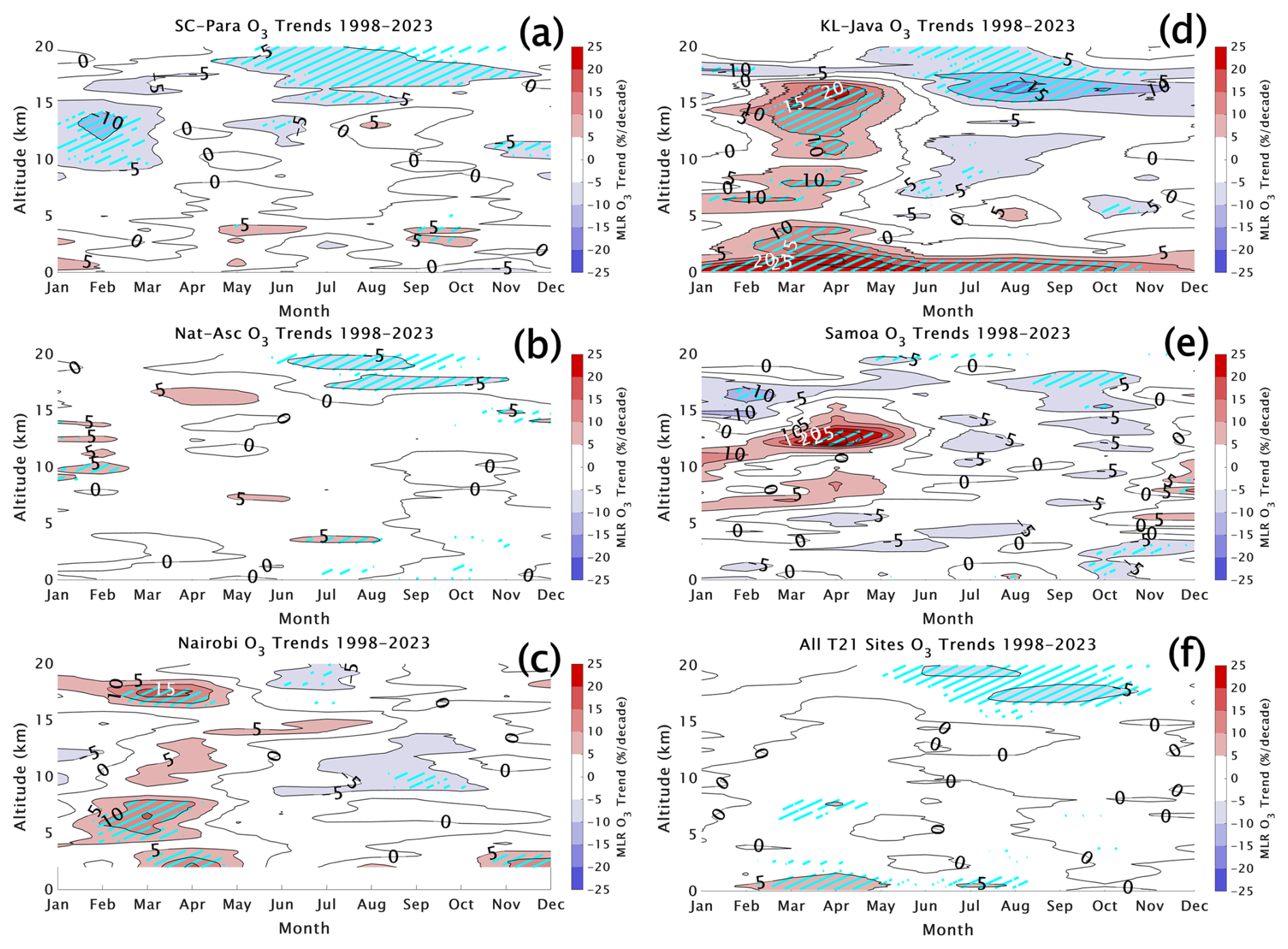
Figure 7 Monthly MLR ozone linear trends from 0 to 20 km in percent per decade for the SHADOZ T21 stations (a) San Cristóbal–Paramaribo (SC-Para), (b) Natal–Ascension (Nat-Asc), (c) Nairobi, (d) Kuala Lumpur–Watukosek (KL-Java) and (e) Samoa. This is an update to Fig. 6 in T21. In (f), average trends over (a) through (e) are displayed by combining the records from all eight individual T21 SHADOZ stations. Positive trends are shown in red shades, and negative trends are shown in blue shades. Trends with p values <0.05 (exceeding the 95 % confidence interval) are shown with cyan hatching.

3.3 FT ozone trends: regional and seasonal variability

3.3.1 Trends for 1998–2023

In Fig. 7 the trends in %/decade computed with MLR at 100 m intervals, for 1998 to 2023, are displayed (update of Fig. 6 in T21 for the 1998–2019 trends). Changes in the ozone column amounts for 1998–2023 computed from the model (DU/decade and %/decade) for the two FT layers (5–10, 10–15 km) appear in Fig. 8. A summary of values for the two layers (and for LMS ozone) appears in Table 2. The percentage values in Fig. 7 and Table 2 are the result of dividing the MLR B(t) term by the A(t) annual cycle of ozone term (Sect. 2.2.1). The MLR-calculated A(t) annual cycle derived from monthly mean ozone profiles (i.e., no anomaly calculation) is used to convert the B(t) trend in ppmv/decade (profiles) or DU/decade (partial columns) to  %/decade. Ozone trends for both percent/decade and DU/decade are given in Table 2. Shades of red (blue) in Fig. 7 represent ozone increases (decreases); cyan hatching denotes trends with p values <0.05. The annual mean trends in Table 2 are computed by taking the average of the 12 monthly trends in DU and dividing by the mean seasonal ozone in DU to yield the annual percentage trend.

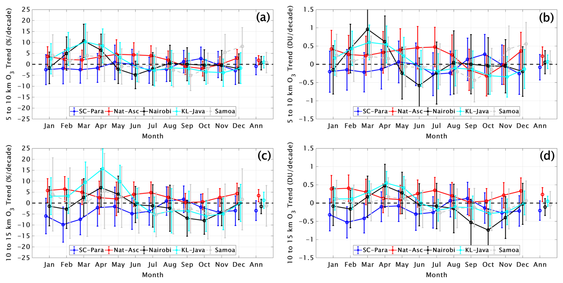
Figure 8 Monthly and annual MLR trends for five T21 SHADOZ sites in lower FT ozone column, integrated from 5–10 km, for (a) %/decade and (b) DU/decade. Panels (c) and (d) are the same as (a) and (b) respectively but for upper FT ozone column (10–15 km), derived from SHADOZ sondes. Dots indicate the monthly and annual (at right in each frame) trends, and error bars display the 95 % confidence intervals.

Figure 9 Summary map of the annual 1998–2023 MLR trends for five T21 SHADOZ sites for the total tropospheric column ozone (TrCO), surface to tropopause, in %/decade from Table 2 including the 95 % confidence intervals.

Figure 10 (a) Monthly MLR trends (colored dots) derived from SHADOZ T21 stations highlighting a July–October decrease in LMS ozone in the 15–20 km layer; yellow dots denote the mean of all T21 stations, with error bars indicating the 95 % confidence intervals. (b) Corresponding TH trends (380 K potential temperature; θ) derived from the radiosondes. (c) Same as (a) except trends have been computed for the segments between the tropopause and 5 km above the TH. Compared to (a) the trends in the tropopause referenced ozone column (c) become close to zero throughout the year.

For three of five stations in Fig. 8a and c, there is a pattern of ozone increase at both FT layers in January to April. Percentage-wise, the greatest increases are at KL-Java and Nairobi, ∼ (10–15) %/decade in March and April. However, SC-Para and Samoa at 5–10 km (Fig. 8a) exhibit almost no trend at any time of year; at 10–15 km SC-Para and Nairobi show losses up to 10 %/decade in February and (5–10) %/decade losses in August and September. However, Table 2 displays no trend on an annual basis for SC-Para and Nairobi. Inspection of Fig. 7 suggests small FT trends at Nat-Asc; Table 2 displays a +3.4 %/decade increase in the 10–15 km layer from 1998–2023. The total column, integrated to the tropopause, TrCO (Fig. 9), over Nat-Asc, has increased (1.9 ± 1.8) %/decade, p<0.05. There are no other annually averaged trends in the FT layers, but TrCO for KL-Java (KL-Watukosek in Table 2) also increased, (2.6 ± 2.3) %/decade (Fig 9).

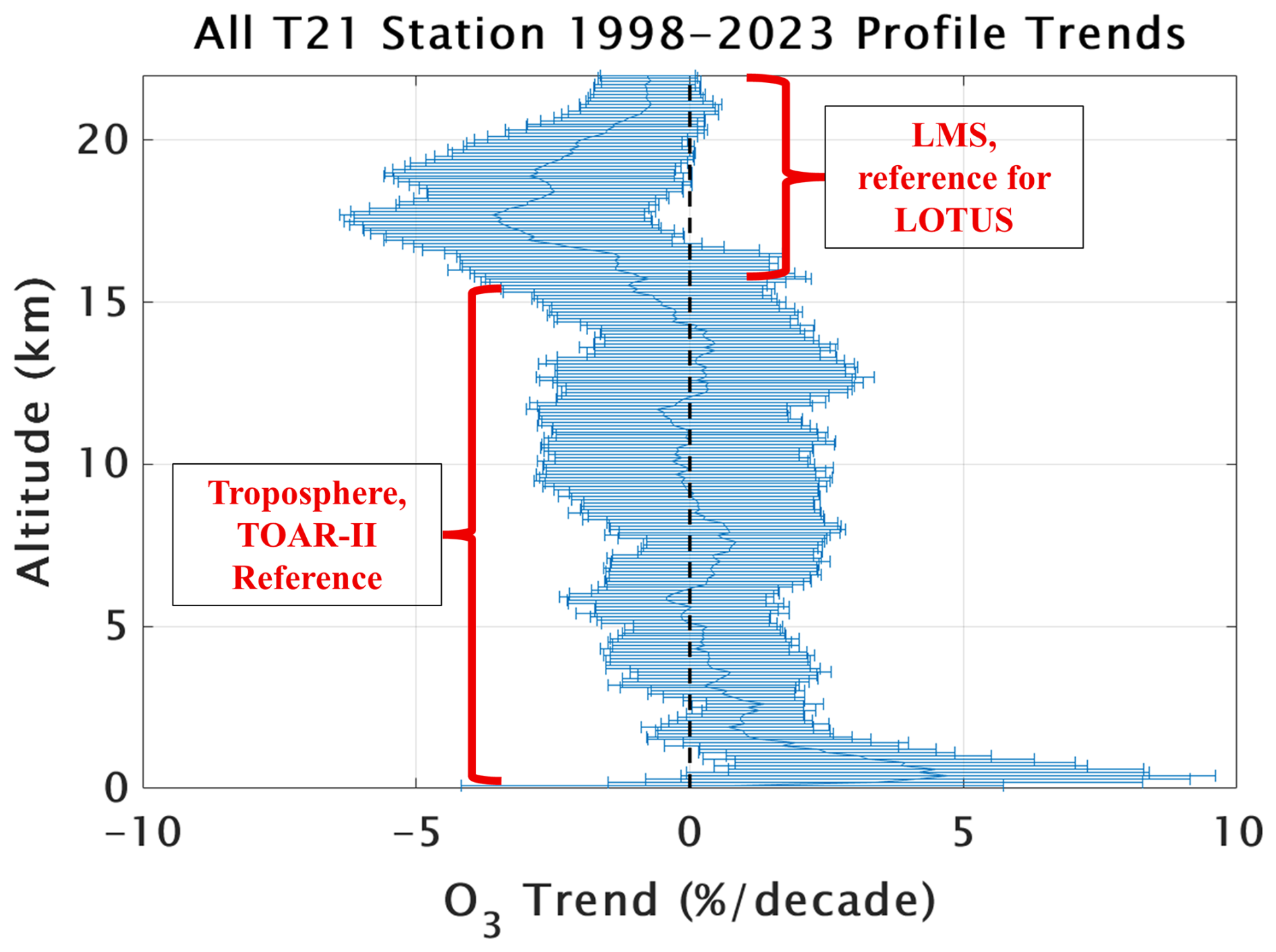
Figure 11 The total mean annual ozone trend (solid blue line), based on mixing ratio changes in 100 m intervals, from the surface to 22 km for all eight T21 SHADOZ profile datasets in %/decade with the 95 % confidence interval range denoted. The LMS region is of interest to the stratospheric community, e.g., the LOTUS activity, whereas the tropospheric segment is marked as the primary TOAR-II focus. The −4 %/decade trend in LMS ozone is similar to that derived from satellites in that region. The mean change throughout the FT is negligible and within the uncertainty range except below 2 km, where mean increases ∼ +5 %/decade are indicated. The near-surface trends are primarily a result of rapid increases in urbanized regions of equatorial SE Asia (Stauffer et al., 2024).

3.3.2 FT ozone trends sensitivity to COVID-19 and 1997–1998 ENSO

A comparison of the Table 2 columns for 1998–2023 relative to those for 1998–2019 (the latter is from T21) reveals little. Only the 10–15 km layer at Nat-Asc has entries with p<0.05 for both periods. The extra 4 years reduced the positive trend slightly. This is consistent with studies that found lingering COVID-related ozone declines in sondes and satellites (Ziemke et al., 2022; HEGIFTOM-1). In Table 2 columns for trends for 2000–2023 can be compared to those for 1998–2023. There is little information in the 2000–2023 column, i.e., no trends anywhere except for the TrCO for KL-Java, an area that was well-studied with satellite and some sonde measurements for the period affected by the large ENSO, amplified by the Indian Ocean Dipole pattern (Thompson et al., 2001). After August 1997, as a result of exceptionally high fire activity, ozone increased greatly. That could have meant a smaller change between ozone levels from 1998 through 2023 which would be consistent with a larger, more robust trend for 2000–2023 (4.6 %/decade for KL-Java) compared to T21, 2.6 %/decade (both p<0.05). Similar trend differences for Kuala Lumpur are also observed with the QR trends in HEGIFTOM-1 (∼ 4–5 %/decade for 2000–2022) versus 2.7 %/decade in Table 4.

Figure 12 FTp column ozone segment anomalies (monthly means) from SHADOZ sondes and IAGOS data, as described in Table 3. Each frame displays the anomalies time series in DU at the left, a histogram of those anomalies in DU (each has a unique scale, ozone anomaly values for each percentile (dashed lines) are in parentheses) and the trend distribution by quantiles. Trends from annual MLR ozone (median, 50th percentile) over 1998–2023 are green circles with their respective ±2σ bars. The same period trends computed with QR by quantiles (0.05= lowest 5th percentile), 0.25 (25th percentile), 0.50 for median trends, 0.75 (75th percentile) and 0.95 (95th percentile) are blue circles. Red circles denote p<0.10. (a) Equatorial Americas, (b) Atlantic and West Africa region, (c) east Africa, and (d) equatorial southeast Asia.

3.4 LMS ozone trends and mean vertical trend over five SHADOZ sites

In T21 (Figs. 10 and 11) trends in the LMS (nominally 15–20 km) showed 5–10 %/decade decreases for Nat-Asc, KL-Java and SC-Para between July and October. For the same months those locations exhibited a tropopause increase ∼ 100 m/decade, suggesting that the seasonal ozone increase is an artifact of a changing tropopause. In other words, if the TH increased, more air with relatively lower ozone would be located in the 15–20 km layer. We tested this hypothesis by recomputing ozone column changes referenced to the TH for 1998–2019, i.e., evaluating trends in a 5 km thick layer above the TH. The result was that the apparent loss of LMS ozone from July to September or October disappeared. The same analyses performed with LMS ozone and TH for the 1998–2023 period (Fig. 10) are the same as for 1998–2019 (T21).

Whatever the cause(s) of ozone loss in the LMS, it is a feature clearly captured by SHADOZ data, as seen in annually averaged ozone trends derived from the analyses displayed in Fig. 11. At 18 km the composite trend from the eight SHADOZ stations analyzed with MLR is (−4 ± 3) %/decade. The mean trend from ∼ 13 to 3 km is zero, albeit with a ± 2σ (95 %) ±  %/decade. Only below ∼ 2 km is the mean ozone trend clearly positive. Most of that increase originates from near-surface pollution over equatorial SE Asia (Fig. 6 in S24).

3.5 Sensitivity tests: trend method, FT sample numbers, and length of time series

3.5.1 Complementarity of trend methods

In Table 4 the median (50th percentile) QR trends from 1998–2023 for the TrCO and FTp ozone segments for the 13 individual SHADOZ stations are presented. The trends for the tropical stations are comparable to the MLR trends in Tables 2 and 3, respectively, within their uncertainties, reaffirming the important HEGIFTOM-1 conclusion; i.e., MLR and QR trends from ground-based data (FTIR and Umkehr, as well as sondes) are essentially the same. In Fig. 12 the time series and histograms show the distribution of IAGOS+SHADOZ ozone anomalies (in DU) for the four regions. The median trends from 1998 to 2023 (50th percentile) for the FTp ozone segments are also displayed with the lowest and highest (5 %, 95 %, respectively) and 25th percentile and 75th percentile quantiles, with red circles denoting p<0.10. The medians are statistically nearly the same, although as expected, the 2σ uncertainty bars are smaller with the QR method than with MLR. The MLR trends are higher in all cases except the Equatorial Americas (Fig. 12a). In the latter case, the positive anomalies have increased significantly for the 5 % and 25 % quantiles over the 26-year period, with no change for the 50 %, 75 % or 95 % quantiles. This signifies that the background (lowest-ozone) air has increasing ozone but the highest-ozone distribution has not changed. Over the Atlantic+West Africa (Fig. 12b) there are also small increases in the lowest part of the distribution, but the median and higher percentiles show no change. Note Natal alone (when not combined with other stations) shows high confidence increases in FTp (and TrCO) ozone (Table 4). East Africa (Fig. 12c) shows marked increases in the lowest-ozone quantiles and the median but a significant decrease in the highest-ozone (more polluted) air. The opposite is true over equatorial southeast Asia (Fig. 12d). The most polluted air corresponds to ozone increasing but the background (lowest ozone) FT segment shows an ozone decrease.

Figure 13 Monthly and annual MLR ozone trends for five combined SHADOZ+IAGOS regions, defined in Table 3, for FTp column in (a) %/decade and (b) DU/decade. Dots indicate the monthly and annual trends, whereas error bars display the 95 % confidence intervals.

3.5.2 FT sample numbers

Figure 13 monthly ozone trends are based on a total of 1.8 times the number of profiles as those in the other lower FT layer, Fig. 8a and b. For the Equatorial Americas (blue) twice as many profiles contribute to the trends in Fig. 13 than in Fig. 8a and b and for Atlantic+West Africa 2.5 times more profiles than in Fig.8a and b. In all four regions, the seasonality of the trends is nearly the same between the 5–10 km FT segment (Fig. 8a and b) and the corresponding SHADOZ+ IAGOS trend (Fig. 13). Furthermore, month by month, the trends are similar to those in the 5–10 km layer in both magnitude and confidence level (uncertainty). Table 3 shows no trends (p<0.05) at any location. The null trends are illustrated in the annual means at the right of each image in Figs. 8 and 13. This was unexpected given the Chang et al. (2023) and Gaudel et al. (2024) suggestions that the uncertainty should decline with more samples and positive trends might be amplified.

Figure 14 The most recent trends, 2005–2023, shown for the equatorial region based on updated OMI/MLS tropospheric total column ozone (TrCO_satellite) estimates in which a ∼ 1 % per decade positive drift in OMI was corrected (a) in DU/decade and (b) in %/decade. The corresponding SHADOZ-derived TrCO_sonde column changes for 2005–2023 are superimposed on the map. Stippling indicates where OMI/MLS trends do not exceed the 95 % confidence interval (i.e., historically referred to as statistically insignificant).

3.5.3 Length of time series

Table 5 displays a comparison of TrCO trends determined by QR for the SHADOZ 26-year period, 1998–2023 for 13 individual SHADOZ stations, and for the same time series only between 2008 and 2019. The uncertainties (expressed as ± 2σ) increased by factors of 2–3 or more for 10 of 13 stations. These results are based on a Comment on Boynard et al. (2025) that also compared the time series changes for 17 mid-latitude ozonesonde stations. Similar uncertainty increases were noted for all 27 stations. Of that total, nine stations exhibited ozone trend sign changes with the 12-year time series although only 10 trends were statistically significant. In Table 5, two stations change sign in their trends, and three stations have a change in confidence level (p<0.05); note that 8 of 13 stations exhibit a substantial change in their trend value, e.g., Samoa and Ascension Island. These results reinforce the need for multi-decade time series.

Table 6 Summary of annual tropospheric (FT, UT and TrCO) ozone trend values for the tropics in ppbv/decade and %/decade with ± 2σ (estimated in some cases where different units are published) from TOAR-II relevant papers separated into five regions: Equatorial Americas, Atlantic and West Africa, East Africa, Southeast Asia, and Samoa. There are six different references, including this work, representing ground-based and satellite observations covering the 1995–2023 time period (note that time ranges vary study to study). NA = not applicable.

^a Note HEGIFTOM data include measurements from the following ground networks: IAGOS, ozonesondes, FTIR, Dobson Umkehr and lidar. ^b Annual average trend plus 2σ. ^c SHADOZ trends have been converted from DU/decade to ppbv/decade for each layer, so these are approximate values based on Tables 1 and 2. ^d OMI/MLS trend values are from the 5×5° box that contains the SHADOZ station. In the cases where there are two SHADOZ stations (Nat/Asc, KL/Java, SC/Para), the trend is the average of the two individual OMI/MLS trends and confidence interval values.

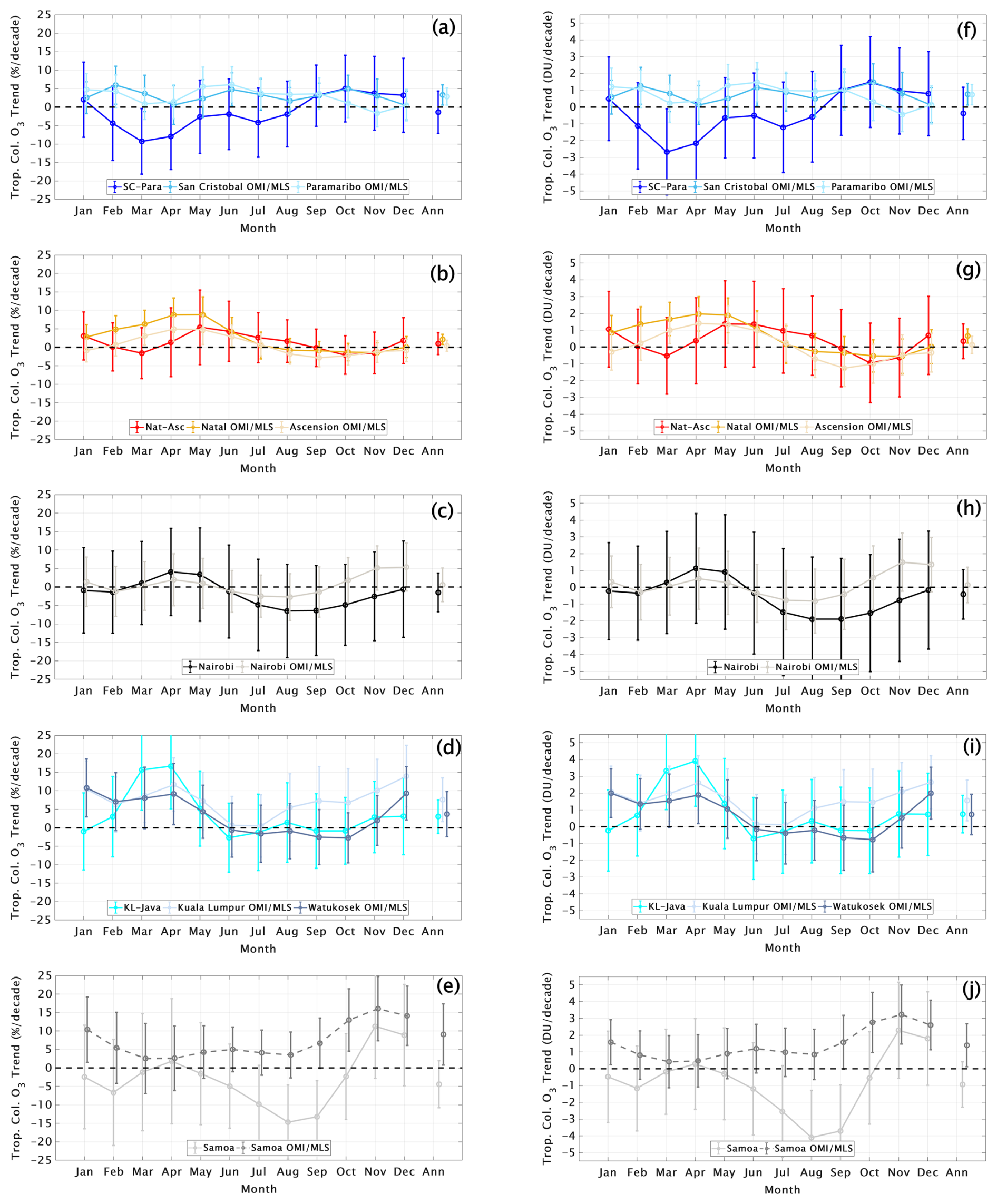
Figure 15 Monthly and annual MLR ozone trends in total tropospheric column (here labeled Trop. Col. O₃), defined using the WMO lapse rate tropopause, for the five T21 stations and the OMI/MLS pixel for each individual SHADOZ station each region. Dots indicate the ozone trend in % (a–e) and DU (f–j) per decade; error bars show the 95 % confidence intervals.

3.6 Total tropospheric ozone trends, TrCO (1998–2023), from OMI/MLS and SHADOZ

Trends for the most recent version of OMI/MLS TrCO_satellite are based on monthly mean satellite data and determined with MLR over the period 2005 through 2023. Trends for total tropospheric column ozone (TrCO_sonde) at the eight SHADOZ sites for the same period appear in circles on the map in Fig. 14, where the stippling indicates no trend can be determined. For both OMI/MLS and the sondes (Fig. 7) shades of red indicate total column ozone increases; blue represents declining ozone over the period of analysis. The mean annual TrCO_sonde trends appear in the two rightmost columns in Tables 2 and 6. In Fig. 14 OMI/MLS shows trends >1 DU/decade (typically 2–9 %/decade) only appear over equatorial SE Asia and parts of South America and the eastern Pacific at ∼ 5° N latitude. Circles indicate locations and trends for the individual SHADOZ stations. The SHADOZ trends display lower trends than OMI/MLS. On a month-by-month basis, the sonde and OMI/MLS trends are compared in Fig. 15. In three cases the seasonality of TrCO trends from sonde and OMI/MLS is similar, and the annually averaged OMI/MLS TrCO_satellite trends are not different from zero (symbols at right of each image). The seasonality of the KL-Java monthly trends agrees well with OMI/MLS; the satellite mean is +5 %/decade (in gray in Fig. 15d). The sonde SC-Para trend (Fig. 15a) is quite a bit lower early in the year than the OMI/MLS trends over San Cristóbal and Paramaribo that average +(2–3) %/decade. The Samoa sonde trend and OMI/MLS TrCO trends diverge most of the year. The satellite annual trend is close to +10 %/decade, an outlier globally (HEGIFTOM-1), as well as over the tropics where no ground-based study results in a significant trend for TrCO_sonde over Samoa (Sect. 4.2).

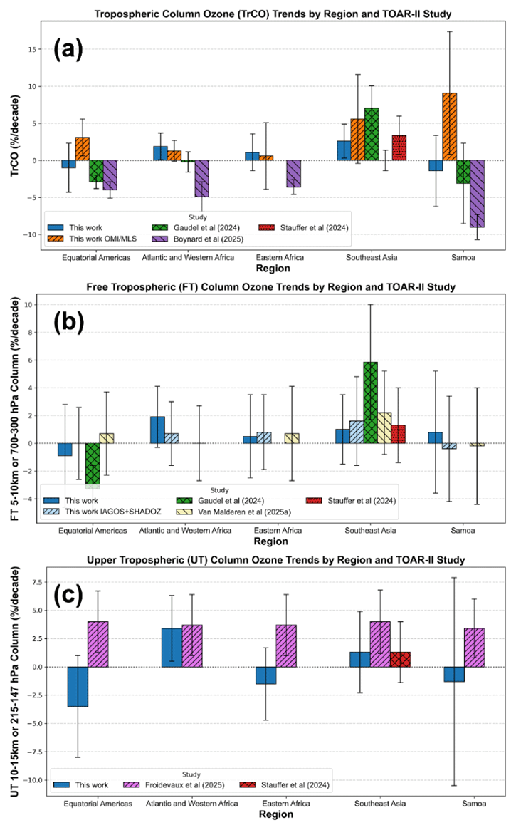
Figure 16 Summary of (a) TrCO, (b) FT, and (c) UT trends from multiple TOAR-II studies (detailed in Table 6). Trends are annual values in %/decade (sometimes estimated from each study); a different color represents each study across (a–c). Note that for trends in (a) and (b), periods differ somewhat: 2004–2019 in Gaudel et al. (2024; Fig. S25); 1998–2022 in Stauffer et al. (2024); 2000–2022 in Van Malderen et al. (2025a); 1998–2023 in This work. All are based on SHADOZ sondes and/or IAGOS. The satellite periods in (c) are 2005–2023 for OMI/MLS, This work; 2005–2020 for MLS in Froidevaux et al. (2025) and 2008–2019 for IASI from Boynard et al. (2025). Error bars show the 95 % confidence intervals. If there are multiple values for a region in one study, a mean value is used.

4 Summary and conclusions

We have presented a two-part evaluation of tropical ozone trends using a 26-year record of ozonesonde (SHADOZ, 1998–2023) profiles with selected FT aircraft (IAGOS) ozone data and the most recent OMI/MLS estimates of tropospheric column ozone for 2005–2023. The next section summarizes the findings. It is followed by Sect. 4.2 which compares our trends to related TOAR II studies. Section 4.3 concludes with a consensus view of FT ozone trends and perspectives relevant to the overall TOAR-II climate and tropical assessments.

4.1 Summary of findings

The first part of the study updates trends in FT and LMS ozone for five stations, Nairobi, Samoa and three combination sites (San Cristóbal–Paramaribo, Natal–Ascension and Kuala Lumpur–Watukosek) extending the T21 trends, that covered 1998–2019, by 4 years. The new analysis added monthly averaged data from 2000 to 2023 to the Goddard MLR model with standard proxies. Trends in FT (5–10, 10–15 km) and LMS (15–20 km) layers are illustrated with monthly means and annually averaged changes in DU/decade and %/decade. Trends determined for the period 2000–2023 assessed impacts of the 1997–1998 ENSO on a possible anomalous starting point. Comparisons of trends for the monthly averaged Aura-derived OMI/MLS total tropospheric column ozone product (TrCO_satellite) were made to those from monthly sonde-derived TrCO_sonde for eight equatorial SHADOZ stations. The principal results of the SHADOZ trend updates and comparisons are as follows:

• The overall characteristics of T21 trends in the FT and LMS are confirmed with 4 additional years of SHADOZ observations. From 1998 to 2023, regional and seasonal variability remains pronounced with FT ozone increasing in thin layers at four of five SHADOZ stations ∼ (5–20) %/decade, mostly between January and May. The exception is at SC-Para where there was a 5–10 % ozone decrease between 10–15 km during 1998 to 2023 compared 5–10 %/decade increases in 1998–2019 (T21). For 1998–2023, the greatest ozone increases occur in multiple layers below 10 km over Nairobi and KL-Java and between 10–15 km over Samoa. However, these features do not translate into annually averaged trends (p<0.05) in the 5–10 or 10–15 km segments except over Nat-Asc; i.e., adding 4 years of data to equatorial SHADOZ data does not modify the T21 picture of little or no FT ozone change. Only when the total tropospheric column (TrCO_sonde) trend is evaluated do Nat-Asc ((1.9 ± 1.8) %/decade) and KL-Java ((2.6 ± 2.3) %/decade) exhibit the slightest trend (p<0.05). Examining the five-station average in vertical form shows a null trend from ∼ 3 to 17 km (0 ± 2 % within 2σ up to 7 km and ∼ 0 ± 3 % from 7 to 17 km). The marginal overall mean increase, +5 %/decade below 3 km, is primarily driven by KL-Java changes.

• With the starting year delayed to 2000, the TrCO_sonde KL-Java trend (2000–2023) is almost twice as large as for 1998–2023, indicating an effect of the 1997–1998 ENSO on equatorial SE Asia. This is not surprising. Watukosek soundings (1997–1998) show ENSO-induced anomalously high ozone over Indonesia that was also captured by satellite tropospheric ozone estimates from TOMS (Thompson et al., 2001).

• The T21 LMS ozone and TH trends are also confirmed with 4 more years of data. For the layer 15–20 km, ozone losses ∼ 5 %/decade from June through October, on average, give an all-site average of −3 %/decade at 17.5 km, a value similar to satellite averages (Godin-Beekmann et al., 2022). As in T21, re-determining the LMS trends for an ozone column 5 km above the tropopause from 1998 to 2023 causes the trend to disappear.

• Annually averaged trends, 2005–2023, determined with MLR for OMI/MLS columns, TrCO_satellite, over the eight individual equatorial SHADOZ stations (members of the five combined sites) and TrCO_sonde overlap within the uncertainties of each. Trends are close to zero at Nat-Asc, Nairobi and KL-Java. The OMI/MLS TrCO_satellite trends are marginally positive at SC-Para, with monthly cycles diverging in the early part of the year at SC-Para. OMI/MLS trends do not capture large monthly seasonal variations seen in SHADOZ profiles, especially for negative trends. The large positive trend from OMI/MLS over Samoa does not align with determinations of FT ozone from this or other studies (see below).

The second part of the investigation was motivated by statistical issues raised in related TOAR II trend analyses. The results of these analyses are summarized:

• Trend methods. The relative merits of trends computed with QR and MLR, previously demonstrated in HEGIFTOM-1, were reinforced with analysis of combined FT SHADOZ-IAGOS data. Although median trends are the same, QR uncertainties are smaller. MLR is superior for capturing seasonal influences, but QR provides vital information on whether the background, low-ozone or high-ozone (polluted) populations are changing the most.

• Sampling frequency. The sensitivity of the 1998 to 2023 FT ozone trends to sample number was explored by using IAGOS profiles to increase the SHADOZ sample size for the equatorial stations by 80 % overall, including a doubling over the Equatorial Americas and Atlantic regions, then applying MLR. Median trends were nearly unchanged. No FT trends over the four regions (plus Samoa) are detected with p<0.05 although uncertainties, expressed in ppbv/decade, improved 30 % over the Equatorial Americas and by ∼ 15 % over three of the four other sites. These results indicate that current SHADOZ sampling with the three combined site records is sufficient in this radiatively important region.

• Length of trends. These were examined for the individual station TrCO_sonde trends by comparing trends for 1998 to 2023 with a 12-year trend (2008–2019), one of two scenarios investigated by Boynard et al. (2025). The uncertainties (as 2σ limits) increase by a factor of 2–3 for TrCO at 10 of 13 SHADOZ stations, and some median trends change sign compared to the 26-year trends (Table 5). The next section shows that even 16-year IASI/Metop trends have an unreasonably low bias with respect to SHADOZ, IAGOS and OMI/MLS trends (Table 6), reinforcing a need for multi-decade datasets where ozone changes are relatively small.

4.2 Comparison of this study to related TOAR-II investigations

How do our tropical tropospheric ozone trends compare to those in other studies that use SHADOZ and IAGOS profiles and/or satellite data? Table 6 summarizes our results for the FT and UT segments and for TrCO. The FT ozone comparisons are made with Gaudel et al. (2024) and with results for two HEGIFTOM studies (HEGIFTOM-1; HEGIFTOM-2). For UT ozone, SHADOZ trends are compared to those derived from the lowest three layers of MLS (Froidevaux et al., 2025; see their Table 2). TrCO trends are taken from the five SHADOZ stations, OMI/MLS (this study) and IASI/Metop (Boynard et al., 2025). Note that the latter study only spans 2008–2023, much less than the SHADOZ data but close to the OMI/MLS period, 2005–2023.

The tropical trend study of Gaudel et al. (2024) groups SHADOZ and IAGOS profiles somewhat differently from this study and only extends through 2019 (period of trends are shown in the fourth column of Table 6). Our trends and those of Gaudel et al. (2024) for FT ozone and TrCO (Table 6; Fig. 16a) for the Equatorial Americas are similar. The Equatorial Americas FT ozone trends range from (−0.01 %)/decade to (−3.3 %)/decade. For TrCO_sonde, derived from profiles, the range is (−1.0 to −3.1) %/decade in between the satellite-based trends: (3.1 ± 2.5) %/decade for OMI/MLS (2005–2023) and (−4.0 ± 1.0) %/decade for IASI/Metop (2008–2023), an offset of 7.1 %/decade for the median trends. Within given uncertainties, IAGOS, IAGOS-SHADOZ-combined and IASI/Metop agree (Fig. 16b).

For the Atlantic and west Africa regions, the profile-based comparisons differ in station-airport combinations among our study, Gaudel et al. (2024) and the two HEGIFTOM analyses. The FT and TrCO trends among the four studies (Table 6, Fig. 16a, b) fall in a relatively small range: (−1.3 ± 2.8) %/decade (FT, Gaudel et al., 2024) to (1.9 ± 1.8) %/decade (TrCO, this study). The larger TrCO from the Natal–Ascension combination appears to result from a higher positive trend in the UT (3.4 ± 2.9) %/decade (Fig. 16c). Because the FT ozone trend of Gaudel et al. (2024) is negative and the Nat-Asc FT ozone trend is positive (Table 6), combining western African IAGOS profiles with the Natal and Ascension measurements, reduces the larger area trend compared to the sonde-only FT ozone trend. Table 6 shows that for all regions the MLS-derived UT ozone trend estimates fall between +3 %/decade and +4 %/decade (Froidevaux et al., 2025). Only over the Atlantic region do any of the SHADOZ UT ozone trends fall in this range. Overall, the Atlantic and West Africa FT ozone and TrCO_sonde trends are (0–2) %/decade, in agreement with OMI/MLS (1.3 ± 1.4) %/decade. As for the Equatorial Americas, the 2008–2023 trends from IASI/Metop over the Atlantic and west Africa are much lower: (−4.9 ± 2.0) %/decade. Compared to the OMI/MLS trend, the IASI/Metop median trend has a 6.2 %/decade low bias. The picture for east Africa (both SHADOZ and IAGOS profiles over Nairobi) is similar to the Atlantic and west Africa. FT ozone, TrCO_sonde and OMI/MLS TrCO trends are essentially null (Table 6, Fig. 16a, b), similar to HEGIFTOM-1, but IASI/Metop displays a (−3.6 ± 1.0) %/decade trend.

There is more variability in trends among the ground-based studies for the equatorial SE Asia region than the Equatorial Americas, Atlantic and Africa, most likely because different combinations of IAGOS profiles and SHADOZ data were used. Supplementing FT KL-Java SHADOZ profiles with IAGOS data (Tables 3 and 6) in our study, a 50 % increase in sample size, did not change the trend appreciably: (1.0 ± 2.6) %/decade vs (1.6 ± 3.2) %/decade. The corresponding TrCO_sonde over KL-Java increased (2.6 ± 2.3) %/decade. S24 computed trends with MLR for KL-Java for 1998–2022: the TrCO_sonde was (3.4 ± 2.6) %/decade. Although the trend period only differs by 1 year, the smaller trend with the extra year in this study (to 2023) might reflect some COVID impact (columns 5 and 7 in Table 2). For OMI/MLS TrCO, determined from a mean of changes averaged over 5°×5° grid boxes for KL and Watukosek (Java), there was a trend of (5.6 ± 6.0) %/decade, 2005–2023. The latter change is nearly the same as Gaudel et al. (2024) for both FT ozone and OMI/MLS changes over the same interval. There are several reasons that Gaudel et al. (2024) FT ozone trends in Table 6 and Fig. 16b are larger than our SHADOZ-IAGOS FT ozone trends. First, the fusing of SHADOZ and IAGOS profiles in Gaudel et al. (2024) may be more heavily weighted to polluted IAGOS segments than our merging. Second, reprocessed IAGOS profiles have not been rigorously compared to SHADOZ data up to this point; a new evaluation of IAGOS instrumentation in the World Calibration Center for Ozonesondes may facilitate consistent referencing to an absolute ozone standard in the future (Smit et al., 2024, 2025). Third, with the shorter trend period, especially ending in 2019, the data of Gaudel et al. (2024) would not be affected by lower, COVID-perturbed ozone concentrations in 2020–2023 as some SHADOZ records are (Table 2).

The HEGIFTOM-1 FT ozone trend (2000–2022) for Kuala Lumpur is nearly identical to the KL-Java trend, 1998–2023: (2.2 ± 3.0) %/decade. In HEGIFTOM-2 (based on SHADOZ KL and IAGOS from several SE Asia airports) FT ozone increases over a longer period (1995–2022) are (6.2 ± 2.2) %/decade. Thus, in general, over SE Asia, as for the Equatorial Americas, Atlantic and Africa, the GB and OMI/MLS trends are in reasonable agreement, given some differences in data selection and in the trend start and end dates: FT and TrCO ozone increases ∼ +(2–8) %/decade. Likewise, the IASI/Metop trend for TrCO, (0.0 ± 1.4) %/decade over 2008–2023 (Boynard et al., 2025), is an outlier over SE Asia.

Nowhere are the satellite data as divergent from the FT sonde trends, near zero change from our study (1998–2023) and Gaudel et al. (2024, for 2004–2019) and HEGIFTOM-1 (2000–2022) than at Samoa (Table 6). TrCO from the SHADOZ sondes has no significant change: (−1.4 ± 4.8) %/decade, this study); (−3.1 ± 5.4) %/decade (Gaudel et al. 2024). However, the OMI/MLS trend for TrCO is (9.1 ± 8.3) %/decade, 2005–2023, and IASI/Metop is (−9.0 ± 1.7) %/decade (Fig. 16a). The large disagreement in trends from sondes and both satellite instruments, the latter with median TrCO trends that are offset by 18 % from one another, underscores the need for profile-based tropospheric ozone trends as an unbiased reference.

4.3 Implications of this study for TOAR II and related assessments

How do our findings apply to an overall TOAR II assessment for tropical ozone? First, there is consensus among the four GB studies: this study, Gaudel et al. (2024) and the two HEGIFTOM articles (HEGIFTOM-1; HEGIFTOM-2). These results provide well-characterized trends in FT ozone for input to climate models and a reference for evaluating TrCO, total tropospheric column ozone trends from evolving tropospheric ozone satellite products. In short, over the past 20–25 years, except for equatorial SE Asia, tropical FT and total ozone trends have been negligible to within ± (1–2) %/decade (Fig. 9). For SE Asia both FT and TrCO have increased from ∼ (2–8) %/decade. Detailed analyses of sonde profiles by S24 suggest that the annually averaged FT ozone trends are (2–3) %/decade. The (5–7) %/decade increases are seasonal in FT ozone. However, for TrCO it is the large ozone increases in the boundary layer found throughout the year that are dominating the total tropospheric column change (Fig. 11).

Second, as far as methods of computing trends, we have shown both the similarity of median trends from QR and MLR and the relative advantages of each with SHADOZ and combined SHADOZ-IAGOS profile data. HEGIFTOM-1 reached similar conclusions about QR and MLR trends for 34 ozonesonde stations, including 10 from SHADOZ. The complementarity of QR and MLR for trend attribution was also highlighted in HEGIFTOM-1. The HEGIFTOM papers (HEGIFTOM-1, HEGIFTOM-2), with a multi-instrument perspective, show variable trends among 55 global stations, including over western Europe and North America where both positive and negative tropospheric column trends occur within a few hundred kilometers. Overall, except for southeast Asia, FT ozone trends from HEGIFTOM are small to moderate and not distinguishable from zero at a number of tropical and extratropical locations.

Third, both HEGIFTOM-1 and this study investigated the matter of sample density in ground-based data, the former by cutting sample size roughly in half for TrCO and our SHADOZ-IAGOS analyses for FT ozone, roughly doubling it. In both studies trend changes determined with MLR were small (a few tenths of a ppbv/decade) and included both increases and decreases (well-illustrated in Fig. S6 in HEGIFTOM-1). Uncertainty changes ranged from 15 %–30 %, usually improving with more sampling. We conclude that arguments for excluding ground-based trends from TOAR II on the basis of sample size have little merit, particularly given ongoing uncertainties and limited record lengths of many satellite products.

Fourth, by reducing the trend period from 26 to 12 years, we quantified the degradation of trends that are too short for the relatively small changes that apply to much of global FT ozone. The length of trends is only one issue for ozone products derived from satellites that have operated less than 2 decades. Trends based on the lowermost levels of ozone from MLS (Froidevaux et al., 2025) were largely the same at all SHADOZ stations, 3–4 %/decade for the UT (Fig. 16c), whereas the sonde-derived trends are geographically variable. Only one of five tropical regions we analyzed, Atlantic and West Africa, displayed a UT ozone trend in this range. The discrepancies between GB-based and satellite ozone trends are not surprising because MLS does not capture observed variability in UT ozone concentrations, up to a factor of 2 between the Atlantic and western Indian Ocean, that is detected by the sondes or UV sensors (Thompson et al., 2003, 2017). We compared our profile-based trends to two typical satellite products: IASI/Metop and the well-characterized OMI/MLS. Within the uncertainty of the satellite trends, OMI/MLS TrCO trends agreed with TrCO_sonde trends in four of five regions. Where sonde-derived trends were near-zero, IASI/Metop trends sometimes agreed well, but for equatorial SE Asia the IASI/Metop zero trend clearly underestimated trends relative to those derived from SHADOZ, SHADOZ-IAGOS combined profiles and OMI/MLS. At Samoa, IASI/Metop (−9 %/decade) and OMI/MLS (+9 %/decade) were both in error, displaying much greater disagreement with the sonde-based trend than anywhere else. There is no easy explanation, but the differing wavelengths, vertical sensitivities and respective biases in the satellite products likely all play a role.

The S24 TOAR-II study is a reminder that the near-zero annually averaged FT ozone trends over most of the tropics (Figs. 8 and 13) in the tropics may mask strong seasonal trends (T21). S24 linked the strong February–April increase in FT ozone over KL-Java (1998 to 2022) to declining convection with four proxies, e.g., outgoing longwave radiation, velocity potential at 200 hPa. A role for changing dynamics must be considered in tropical tropospheric ozone increases; increasing ozone precursor emissions are apparently not the only driver. In a similar manner, decreases observed in LMS ozone appear to be related to tropopause height changes during the 1998 to 2023 period.

In summary, our updated results for SHADOZ stations (Figs. 9 and 11) remain the most reliable reference for trends throughout the tropical troposphere and LMS. We provide a definitive standard for evaluating monthly trends and regional variability of satellite-based products and related models being used for tropical ozone trends over the past 25 years. Together with the more extensive HEGIFTOM and IAGOS coverage, our SHADOZ analyses lead to a conclusion that the most reliable trend information for TOAR II is based on re-processed GB measurements. However, coverage of the ground-based instruments is uneven, and space-based observations are needed for truly global trends. In order for satellite products to mature and for differences among them to be understood, independent ozone data collection, particularly from ozonesondes referenced to an absolute standard, is required. As our investigations with the high-resolution SHADOZ profiles have demonstrated, sonde data will remain the gold standard for deriving trends in the FT and LMS, the two most critical regions where ozone interacts with the climate system.