Hunting for gravity waves in non-orographic winter storms using 3+ years of regional surface air pressure network and radar observations

Atmospheric gravity waves (i.e., buoyancy waves) can occur within stable layers when vertical oscillations are triggered by localized heating, flow over terrain, or imbalances in upper-level flow. Case studies of winter storms have associated gravity waves with heavier surface snowfall accumulations, but the representativeness of those findings for settings without orographic precipitation has not been previously addressed.

We deployed networks of high-precision pressure sensors from January 2020 to April 2023 in and around Toronto, ON, Canada, and New York, NY, USA, two regions without strong topographic forcing. Pressure wave events were identified when at least four sensors in a network detected propagating pressure waves with wave periods ≤67 min, wavelengths ≤170 km, and amplitudes ≥0.45 hPa. Reanalysis model output and operational weather observations provided environmental context for each gravity wave event. We detected 33 pressure wave events across 40 months of data; of these events, 23 were gravity waves, whereas the rest were frontal passages, outflow boundary passages, or a wake low. We found a strong linear relationship between amplitude and event duration for the 23 atmospheric gravity wave events.

Gravity wave events are rare in non-orographic snow storms in our study region. Of the 594 h with ≥0.1 mm h⁻¹ (liquid equivalent) of snow sampled, only 19 h was during a gravity wave event. When gravity waves and enhanced reflectivity bands within snow co-occurred, the bands did not move in a direction or at a velocity consistent with the pressure waves. In agreement with previous work, most of our gravity wave events are associated with strong upper-level flow imbalances to the south or west of their location.

1 Introduction

Atmospheric gravity waves (i.e., buoyancy waves) result from the forced perturbation of air parcels in a statically stable environment such that parcels oscillate about their original height, with parcel buoyancy acting as the restoring force (Nappo, 2002). Possible triggering mechanisms for gravity waves can include, but are not limited to, forced flow over topography, adjustment to imbalanced flow, and localized latent heating (Fritts and Alexander, 2003). The resulting up and down motions can propagate outwards from the location of their originating triggering mechanism through stable layers, but they do not yield net movement of fluid, nor do they necessarily follow the mean flow of the air through which they propagate.

Case studies of winter storms have associated gravity waves with heavier surface snowfall, but the representativeness of these findings for settings without strong topographic forcing has not been systematically examined. It is the goal of this paper to remedy that gap with a comprehensive analysis of observed gravity waves based on 40 months of pressure sensor network data. The waves that we present in this paper are propagating (i.e., not terrain-locked), are of moderate to high amplitude (up to 5.5 hPa, in a similar range to Uccellini and Koch, 1987), have short to moderate wavelengths (up to 170 km), and have short to moderate wave periods (up to 67 min). The types of disturbances that were detected by our networks of pressure sensors included not only gravity waves but also synoptic fronts, convective outflow boundaries, and a convective wake low. We will describe how we discerned these four types of disturbances from one another in Sects. 2.2 and 2.3. In order to keep terminology clear and consistent, and because different studies may use different conventions, Table 1 defines the terms used in this paper, which are related to both wave properties and the different types of waves.

Miller et al. (2022)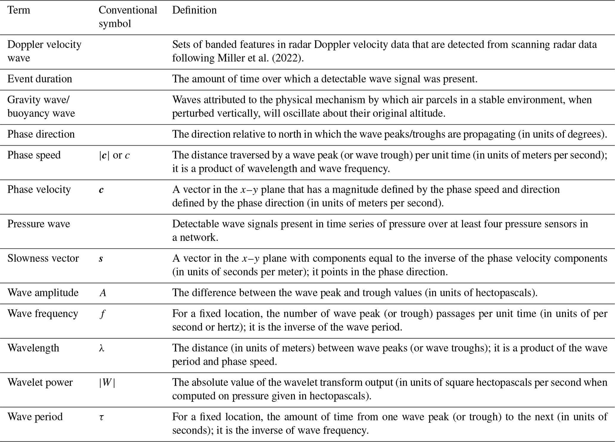

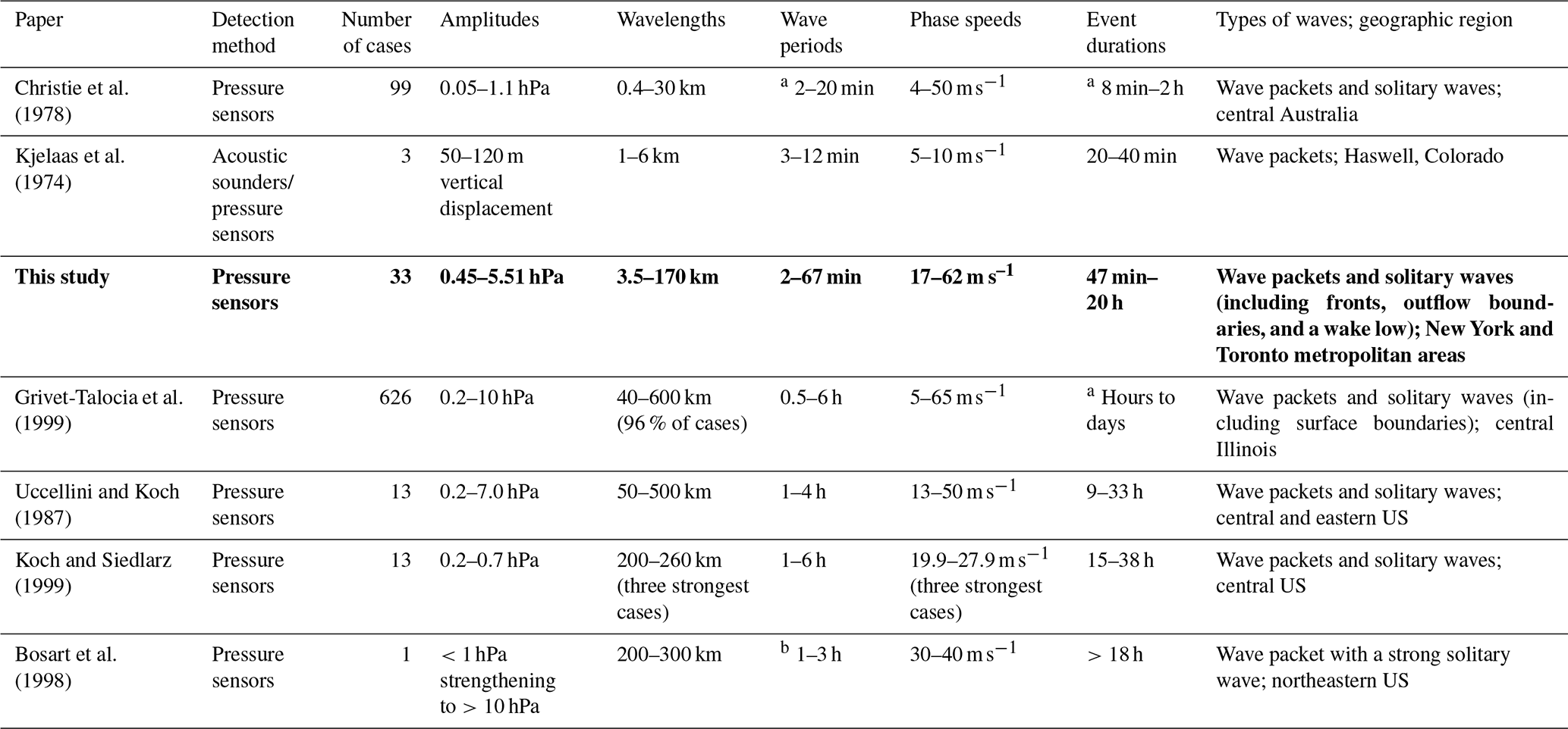
Table 1 Definitions of key terms used in this paper.

Many observational studies have used pressure sensors to detect gravity wave signals (e.g., Kjelaas et al., 1974; Christie et al., 1978; Uccellini and Koch, 1987; Einaudi et al., 1989; Bosart et al., 1998; Grivet-Talocia et al., 1999; Koch and Siedlarz, 1999). In this study, we use networks of high-precision pressure sensors to detect and track gravity waves and analyze them in the context of radar-detected features in winter storms. Table 2 compares the properties of the waves presented in this paper to those in a selection of other papers from the literature. The spatial scales and timescales of pressure waves that we focus on, 3.5 to 170 km and 2 to 67 min, respectively, overlap the upper end of the scales examined in previous work by Christie et al. (1978) and the lower end of the scales examined by Grivet-Talocia et al. (1999) and Uccellini and Koch (1987).

Table 2 Properties of pressure waves presented in this study (indicated in bold) and in some prior studies and meta-analyses from the literature. Rows are in ascending order by minimum wavelength. Information in cells indicated with ^a were inferred from figures in the associated paper (not directly stated), and the cell indicated with ^b was inferred from the wavelength and phase speed range for that paper.

1.1 Possible effects of gravity waves on cloud and precipitation processes

Gravity waves can have noticeable effects on cloud and precipitation processes under a subset of conditions within the troposphere. In marine stratocumulus, upward motions associated with gravity waves can yield enhancements in drizzle (Allen et al., 2013; Connolly et al., 2013). In the southeast Atlantic, satellite observations have revealed cases of marine stratocumulus cloud decks rapidly eroding, and this abrupt cloud-clearing effect appears to be related, at least in part, to gravity waves (Yuter et al., 2018; Tomkins et al., 2021). In deep convection, latent heating can trigger gravity waves of varying frequency that alter the pre-storm environment and lead to the initiation of convection ahead of the existing line of storms, often referred to as “action at a distance” (Fovell et al., 2006; Adams-Selin, 2020) and “gregarious convection” (Nicholls et al., 1991; Mapes, 1993; McAnelly et al., 1997). There has also been extensive work describing mechanisms whereby terrain-locked gravity waves can enhance clouds and precipitation (e.g., Gaffin et al., 2003; Colle, 2004; Doyle and Durran, 2007; Houze, 2012, 2014; Kingsmill et al., 2016; Ma et al., 2023).

In order for gravity waves to modify clouds and precipitation, several processes have to occur in sequence under suitable conditions (Fig. 1). Gravity waves are first triggered. Following this, the waves propagate away from their source location and may be ducted. If cloud is not already present in the wave duct, the upward branches of the gravity waves must lift parcels to saturation, either with respect to ice (for an air temperature <0 °C) or with respect to liquid water (for an air temperature ≥0 °C), in order for cloud to form. If conditions are saturated or supersaturated in the wave duct (either RH_ice≥100 % and/or RH_water≥100 %), enhanced vapor deposition and/or condensation can occur in the upward branches of gravity waves. If lifting associated with a gravity wave brings an ice- or mixed-phase cloud parcel to liquid water saturation and if riming then occurs, that rimed ice mass will not be removed from particles unless RH_ice falls below 100 % in the downward branch of the gravity wave and sublimation occurs. When net increases in particle mass due to gravity waves are sufficient to enlarge cloud particles to precipitation-sized particles, the precipitation that falls out of the parcel results in a net loss of total water from the parcel that is not reversible (e.g., Allen et al., 2013).

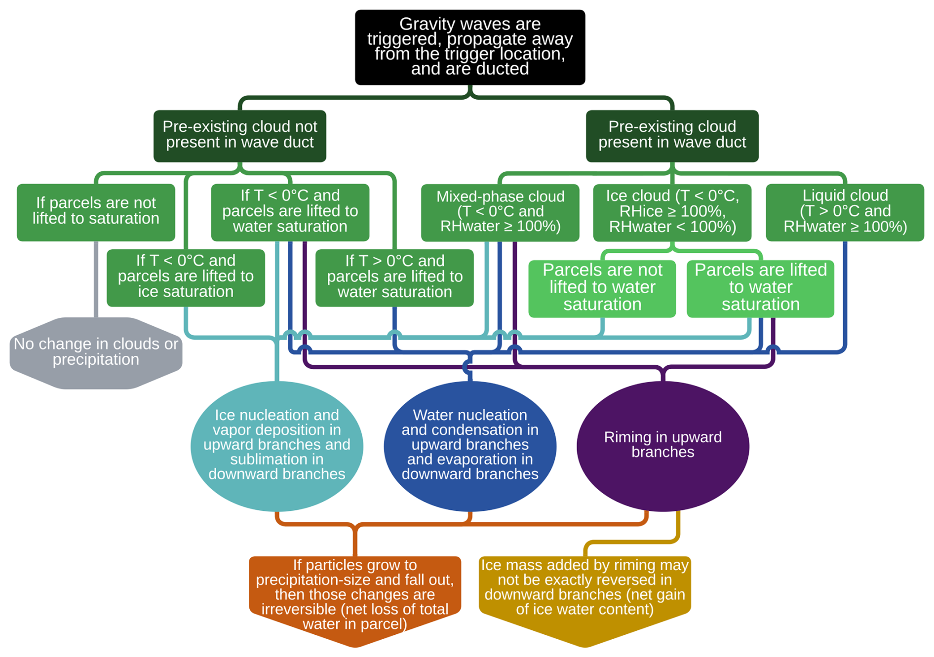
Figure 1 Possible chains of processes and outcomes for gravity waves to yield changes in cloudiness and precipitation. The sequence goes from top to bottom. Green rectangles indicate conditions or requirements, ovals indicate microphysical processes that result from the air motions associated with gravity waves, and downward-pointing pentagons indicate irreversible changes within air parcels resulting from the previous steps. For simplicity, sequences in which air parcel temperatures cross the 0 °C level altitude are not shown.

1.2 Gravity waves in winter storms: case studies

Previous case studies of gravity waves in winter storms include those that are close to the scale range targeted by this study (wavelengths ≤170 km and wave periods ≤67 min) and those that examined larger-scale phenomena. Gaffin et al. (2003) described a heavy-snowfall event during which gravity waves generated by flow over terrain in the lee of the Smoky Mountains contributed to localized lifting. Bosart et al. (1998) presented a case of a very large amplitude gravity wave (with a peak-to-trough pressure difference on the order of 10 hPa) associated with observed snowfall rates of up to 15 cm h⁻¹ (this refers to snow depth, not liquid equivalent) in the northeastern US on 4 January 1994. The gravity wave in this case propagated at roughly 30–40 m s⁻¹ toward the northeast with a wavelength of 200–300 km (implying a wave period of roughly 1.4–2.8 h). Zhang et al. (2001) simulated the 4 January 1994 case presented by Bosart et al. (1998) using the National Center for Atmospheric Research/Pennsylvania State University Mesoscale Model 5. Their analysis of the simulated case indicated that geostrophic adjustment in the exit region of an upper-level jet streak initially triggered lower-amplitude gravity waves (roughly 1 hPa from peak to trough), which merged and had a resonant interaction with an upper-level front, leading to their nonlinear amplification. Zhang (2004) later generalized the term “geostrophic adjustment” to “balance adjustment” for curved flows as the trigger for gravity wave genesis. In the model results shown by Zhang et al. (2001), the upward motion associated with the interaction of the gravity wave and the upper-level front led to the release of potential instability and a region of elevated convection, where heavy precipitation was produced in the simulation. While past studies such as Bosart et al. (1998) have focused on individual cases in which gravity waves were associated with heavy snowfall, there are remaining questions regarding how common that association is for typical winter storms in the northeastern US and southern Canada.

The conditions necessary for gravity wave generation by balance adjustment often exist in the strong baroclinic trough–ridge systems which produce winter storms. After gravity waves are generated aloft, their energy propagates upward and downward. If appropriate conditions exist, the waves can then be ducted or trapped within a cloud layer, allowing the waves to influence cloud processes (Ruppert et al., 2022). Lindzen and Tung (1976) described the theoretical conditions for an ideal wave duct: an absolutely stable ducting layer (where the environmental lapse rate < the moist adiabatic lapse rate) beneath a statically neutral or conditionally unstable reflecting layer (where the environmental lapse rate ≥ the moist adiabatic lapse rate). Such lapse rate conditions are common ahead of a warm/stationary front or behind a cold front (e.g., Uccellini and Koch, 1987).

1.3 Reflectivity bands and velocity waves in winter storms

Gravity waves have been previously suggested as the key mechanism yielding locally enhanced bands of radar reflectivity in snow and parallel sets of waves in Doppler velocity. Detection of wave signals using an array of pressure sensors can help distinguish gravity waves from the other candidate processes (Sect. 8.2 in Nappo, 2002).

Linear regions of locally enhanced radar reflectivity (bands) are frequently observed in winter storms (e.g., Novak et al., 2004; Hoban, 2016; Ganetis et al., 2018). These bands are conventionally categorized into two types: a primary band and sets of multibands. Winter storms have been found to contain both a primary band and multibands, only a primary band, only multibands, or no bands at all (Hoban, 2016; Ganetis et al., 2018). Primary bands are ≥200 km long, usually 30–70 km wide, occur as a single feature in reflectivity within a given storm, and have been associated with regions of strong frontogenesis along an occlusion (Novak et al., 2004; Baxter and Schumacher, 2017; Ganetis et al., 2018). Multibands are <200 km long, usually 10–50 km wide, and occur in groups of two or more bands, which are often roughly evenly spaced (Hoban, 2016; Ganetis et al., 2018).

Ganetis et al. (2018) found no robust correspondence between frontogenesis and the occurrence of multibands. Processes that may lead to multibands include gravity waves (Gaffin et al., 2003; Hoban, 2016), Kelvin–Helmholtz waves (Houser and Bluestein, 2011), shear-organized lines of cloud-top generating cells (Keeler et al., 2016, 2017), and convective cells elongated by flow anomalies resulting from potential vorticity dipoles (Leonardo and Colle, 2023).

The snowfall accumulation associated with a reflectivity band is a function of the intensity (i.e., snowfall rate) and the duration that the band is over a fixed location. The snowfall rate does not monotonically increase with reflectivity (Fujiyoshi et al., 1990; Rasmussen et al., 2003), so measuring band intensity from radar data alone has large uncertainties. Reflectivity in snow can be increased by the aggregation or partial melting of ice particles, which would not increase the associated snow mass. Additionally, localized reflectivity enhancements observed by radar a few kilometers above the surface may not reach the surface (Tomkins, 2024). Given ground-relative propagation speeds on the order of 10–30 m s⁻¹ in the band-perpendicular direction, enhanced reflectivity bands usually pass over a given location in 5–120 min. Longer durations over a location are possible when there is a band-parallel component to the motion.

Hoban (2016) and Miller et al. (2022) identified waves in the Doppler velocities (“Doppler velocity waves”) measured by National Weather Service Next Generation Weather Radar (NEXRAD) system radars (WSR-88Ds) in the northeastern US during winter storms using the difference field between successive radar scans. Hoban (2016) analyzed 71 winter storms that contained multibands. Of those 71 storms with multibands, 50 also contained coherent sets of propagating Doppler velocity waves. If the sets of propagating parallel Doppler velocity bands have a surface pressure signal, they could be gravity waves; if not, other mechanisms such as Kelvin–Helmholtz waves are more likely.

1.4 Objectives of this study

In this study, we use high-precision surface pressure sensors to objectively identify pressure wave events over a 40-month period, characterize the wave properties and their synoptic environments, and examine whether and how often the pressure waves are related to enhancements in radar reflectivity and coherent sets of Doppler velocity waves. Section 2 describes the pressure data and processing techniques to extract wave events; the reanalysis model output used to characterize the large-scale environment; and the several types of observations used to identify enhanced reflectivity bands, Doppler velocity waves, temperature inversions, and surface snow rates. Section 3 describes the characteristics of pressure wave events and their environmental context. In Sect. 3.1.3, we discuss the pressure waves in the context of radar-detected features, including how often they were co-located and moving with enhanced reflectivity bands and/or Doppler velocity waves. Finally, Sect. 4 includes conclusions and discussion of the results with potential avenues for future work.

2 Data and methods

We used networks of pressure sensors in the Toronto (ON, Canada) and New York (NY, USA) metropolitan areas to detect wave events (Allen et al., 2024d, and Fig. 2), and we analyzed the context of those wave events using ERA5 reanalysis data (Hersbach et al., 2020), radiosonde data from the Integrated Global Radiosonde Archive (IGRA; NOAA National Centers for Environmental Information, 2021b), surface weather data from the Automated Surface Observing Systems (ASOS; NOAA National Centers for Environmental Information, 2021a), and operational S-band radar data from the US National Weather Service (NWS) WSR-88D radars (NEXRAD; NOAA National Weather Service Radar Operations Center, 1991).

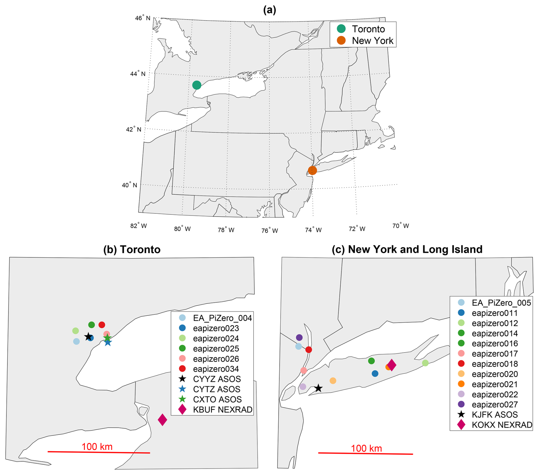
Figure 2 Maps of the pressure sensor, ASOS, and radar sites used in this study. (a) Locations of Toronto and New York City. (b) Pressure sensor sites in Toronto (filled circles) with the three ASOS sites (stars) and KBUF radar (maroon diamond). (c) Pressure sensor sites in New York and Long Island (filled circles) with the KJFK ASOS (black star) and KOKX radar (maroon diamond).

2.1 Pressure sensor data

In numerical model output, gravity waves can be identified by analyzing the 3D gridded fields of pressure, geopotential height, wind, and temperature perturbation values. In observations, gravity waves can be implied from the presence of ripples in satellite-observed cloud tops and in Doppler velocity data observed by radar and lidar (e.g., Miller et al., 2022). However, similar ripple-like structures can occur with Kelvin–Helmholtz waves (Houser and Bluestein, 2011). To definitively distinguish between gravity waves and Kelvin–Helmholtz waves, pressure sensor data are needed (e.g., Christie, 1992). Gravity waves will have a pressure wave signature, whereas Kelvin–Helmholtz waves will not. Not all pressure waves are gravity waves (Allen et al., 2024d).

We deployed high-precision pressure sensor networks in the Toronto (ON, Canada) and New York (NY, USA) metropolitan areas over a 3-year period (sensor locations shown in Fig. 2). To minimize the cost and hassle, these sensors were located in the homes and offices of our collaborators and automatically reported back to a server at North Carolina State University where the data were archived.

Each instrument utilized either a Bosch BME280 (Bosch, 2022) or a Bosch BMP388 (Bosch, 2020) pressure sensor, and the timestamps, data logging, and communications were handled by Raspberry Pi Zero single-board computers (Allen et al., 2024d). Each sensor was placed indoors to minimize wind contamination in the pressure measurements. The noise floor of the sensors is roughly 0.8 Pa, depending on ambient conditions. The sensors continuously recorded pressure at 1 s intervals when possible, but power or internet outages occasionally caused gaps in the data record (Fig. 3). We analyzed data between January 2020 and April 2023. Most of the sensors in New York and Long Island were deployed prior to January 2020, while the sensors in Toronto were deployed starting in October 2020 (Fig. 3). Analysis subsequent to the deployment of the sensors suggests that the smaller spatial scale and more circular pattern of the Toronto network, compared with the larger spatial scale and more linear west–east arrangement of the sensors in New York (Fig. 2), likely makes the Toronto network better at detecting smaller-amplitude pressure waves.

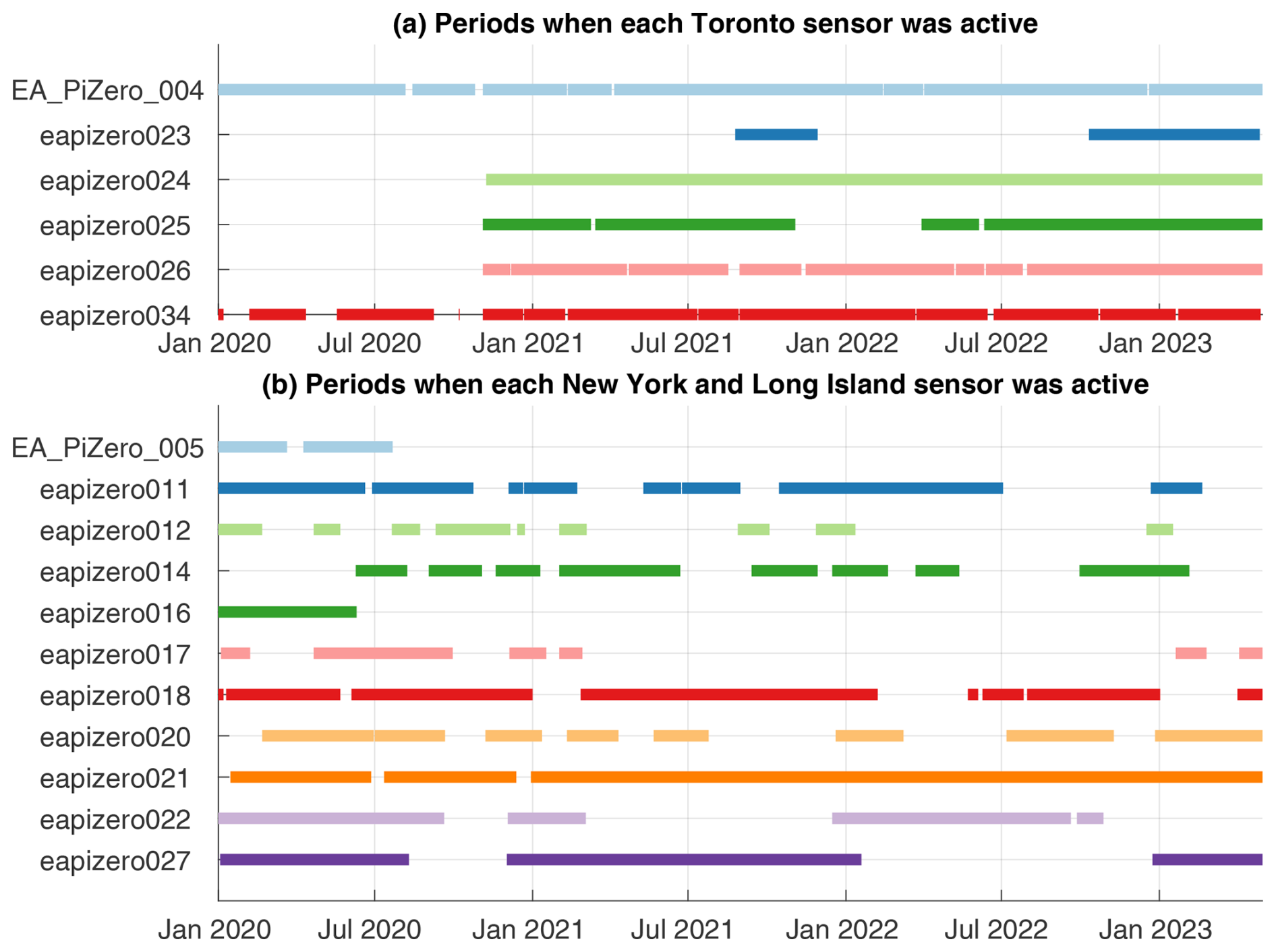
Figure 3 Timelines of when the pressure sensors in (a) Toronto and (b) New York and Long Island recorded pressure data between January 2020 and April 2023.

2.1.1 Detection of wave events

Allen et al. (2024d) described the methods for detecting waves in the pressure sensor data in detail; therefore, the technique is only summarized here. To smooth out artifacts and high-frequency pressure variations, we use 10 s samples of pressure in hectopascals (i.e., we take the 10 s moving average then use every 10th point of the smoothed time series). The detection method relies on a wavelet transform, a technique for identifying wave signals in time–wave period (or time–frequency) space, which is preferable to Fourier transforms for finding transient (i.e., time-localized) waves. We used an analytic morse wavelet (Olhede and Walden, 2002; Lilly and Olhede, 2012) and analyzed wave periods between 1 and 120 min to detect waves on similar temporal scales to enhanced reflectivity bands. The output of the wavelet transform is an array of complex values in time–scale space. The absolute value of those values is referred to as the wavelet power ($\left|W\right(b,a\left)\right|$, in units of hPa² s⁻¹).

Mean wavelet power increases with scale (i.e., wave period; Fig. 5 in Allen et al., 2024d). Therefore, the threshold defining wave events should also vary with scale. A scale-dependent threshold function A(a) was defined using the mean wavelet power across the full data set by scale, multiplied by a constant K:

$$\begin{array}{}\text{(1)}& A\left(a\right)=K{〈\left|W\right(b,a\left)\right|〉}_b.\end{array}$$

To identify robust wave signals with large enough amplitudes to potentially modify cloud and precipitation processes, we used K=10. A lower threshold could lead to the detection of many weak wave events, which may then be erroneously paired across multiple sensors when they were separate wave events in reality. Wave events were then identified as peaks in the wavelet power that exceeded A(a), along with their connected regions that exceeded $\frac{A\left(a\right)}{\mathrm{2}}$. We refined these regions using the watershed transform to separate distinct signals at different wave periods and then took the bounding box to obtain the final event regions. Following this, the wavelet transform was inverted over the final event region to extract the wave event trace (Allen et al., 2024d).

After wave event traces were extracted for each sensor individually, we identified coherent wave events across multiple sensors using the cross-correlation function C_ij(Δt):

$$\begin{array}{}\text{(2)}& C_{ij}\left(\mathrm{\Delta }t\right)={\displaystyle \frac{\mathrm{1}}{\Vert p_i\Vert \Vert p_j\Vert }}\int p_i\left(t\right)p_j(t+\mathrm{\Delta }t)\mathrm{d}t,\end{array}$$

where p_i(t) and p_j(t) are the respective extracted wave event traces for sensors i and j. Events in pairs of sensors were matched together if the maximized C_ij(Δt) value exceeded 0.65, with the time between wave passages at the two sensors estimated by the corresponding time lag Δt_opt (in seconds). The cross-correlation function and associated Δt_opt values were calculated for each possible pair of sensors within a network, which produced a vector of time lags t representing the time between wave passages at each pair of sensors that captured the event.

We then calculated the slowness vector using the time lags t for each wave event. The slowness vector is a two-element vector $\mathit{s}=(s_x,s_y)$, where s_x and s_y (in s m⁻¹) are the inverses of the x and y components of the wave phase velocity, $\frac{\mathrm{1}}{c_x}$ and $\frac{\mathrm{1}}{c_y}$ (in m s⁻¹), respectively. We solve for s starting from the following equation (Del Pezzo and Giudicepietro, 2002):

$$\begin{array}{}\text{(3)}& \mathit{t}=\mathit{s}\cdot \mathbf{\Delta }\mathit{x},\end{array}$$

where Δx is the two-column matrix of the x and y components of the distance vectors (in meters) between each pair of sensors that captured the event. For events captured by at least three sensors, Eq. (3) represents an overdetermined system of linear equations, from which s is estimated using a least-squares approach:

$$\begin{array}{}\text{(4)}& \mathit{s}=(\mathbf{\Delta }{\mathit{x}}^{\mathrm{T}}\mathbf{\Delta }\mathit{x}{)}^{-\mathrm{1}}\mathbf{\Delta }{\mathit{x}}^{\mathrm{T}}\mathit{t},\end{array}$$

where superscript T indicates the transpose of a matrix (Del Pezzo and Giudicepietro, 2002). The components of the slowness vector are then inverted to obtain the wave phase velocity vector $\mathit{c}=(c_x,c_y)$. We assessed this phase velocity estimate by calculating the “modeled” delay times t_m using Eq. (3) with the estimated slowness vector. We calculated the root-mean-square error (RMSE, in seconds) and normalized root-mean-square error (NRMSE, unitless) of the modeled delay times as follows:

$$\begin{array}{}\text{(5)}& {\displaystyle }\text{RMSE}=\sqrt{{\displaystyle \frac{{\sum }_{i=\mathrm{1}}^{N_{\mathrm{s}}(N_{\mathrm{s}}-\mathrm{1})/\mathrm{2}}(t_{\mathrm{m},i}-t_i{)}^{\mathrm{2}}}{N_{\mathrm{s}}(N_{\mathrm{s}}-\mathrm{1})/\mathrm{2}}}},\text{(6)}& {\displaystyle }\text{NRMSE}=\sqrt{{\displaystyle \frac{{\sum }_{i=\mathrm{1}}^{N_{\mathrm{s}}(N_{\mathrm{s}}-\mathrm{1})/\mathrm{2}}(t_{\mathrm{m},i}-t_i{)}^{\mathrm{2}}}{{\sum }_{i=\mathrm{1}}^{N_{\mathrm{s}}(N_{\mathrm{s}}-\mathrm{1})/\mathrm{2}}(t_i{)}^{\mathrm{2}}}}},\end{array}$$

where N_s is the number of sensors that captured a given event.

To have reasonable confidence in the wave phase velocity estimate for a given event, we require the event to be captured by at least four sensors with an RMSE below 90 s and an NRMSE below 0.1. These thresholds are based on the analysis in Allen et al. (2024d). We consider an RMSE on the order of hundreds of seconds to be unacceptably large, and after analyzing all wave events captured by four or more sensors, we found an RMSE=90 s and an NRMSE=0.1 to be a break in the data. Additionally, the following results exclude any wave events found between 15 January and 18 January 2022, following the Hunga Tonga volcanic eruption on 15 January 2022, which produced a Lamb wave with measurable pressure signals globally (Adam, 2022; Burt, 2022; Allen et al., 2024d). After applying those criteria, 33 total trackable pressure wave events were detected by the Toronto and New York pressure sensor networks between January 2020 and April 2023. A total of 19 pressure wave events were detected by the Toronto pressure sensor network, whereas 14 were detected by the New York pressure sensor network (Table 3).

Table 3 Properties of the 33 pressure wave events detected over the 40-month analysis period. The leftmost column is an index column. In the location column, “TOR” indicates the Toronto sensor network, and “NY” indicates the New York and Long Island sensor network. The wave period and amplitude are averaged among sensors that detected a given event. Phase direction is shown in degrees clockwise from northward (e.g., 90° indicates a wave propagating from west to east). Rows in bold indicate gravity wave events.

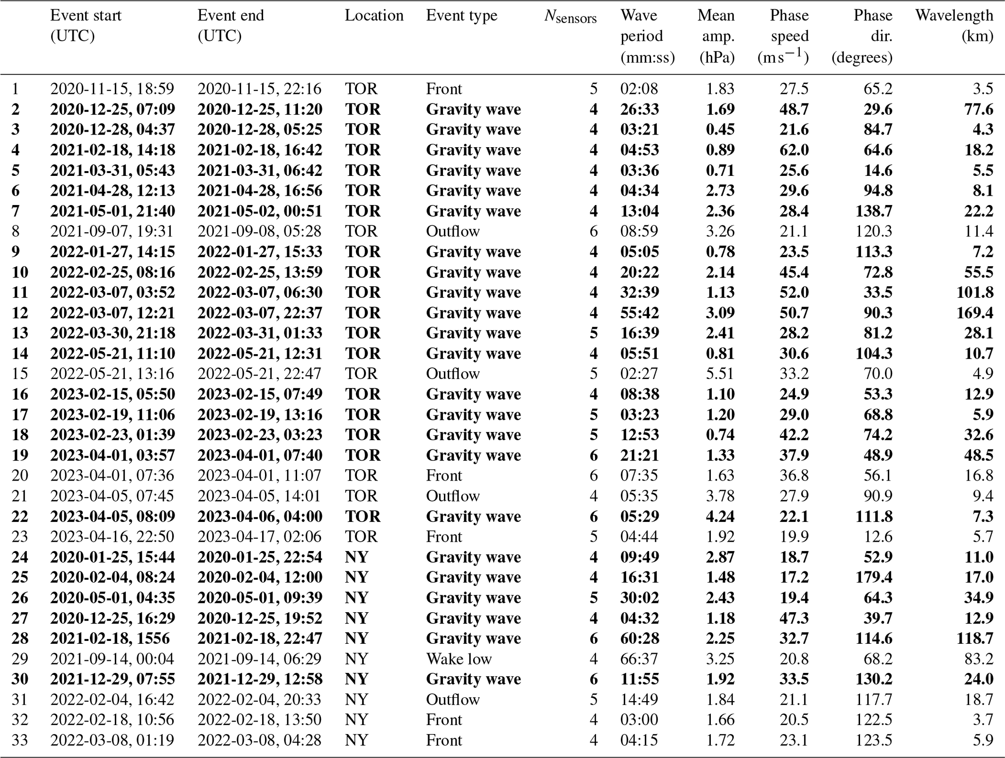
In general, pressure waves of amplitude above roughly 0.1 hPa could be detected in a single sensor, depending on the wave period (shorter waves had a lower detection threshold). However, the waves with lower amplitudes (i.e., weaker signals) were more difficult to track across multiple sensors. As a result, each of the trackable pressure waves in this study had an amplitude of at least 0.45 hPa. Table 2 compares this amplitude to other studies in the literature, which found pressure waves between 0.05 and 10 hPa in amplitude.

2.2 ERA5 reanalysis data

We used hourly ERA5 reanalysis data (Hersbach et al., 2020) to characterize the large-scale environment near the surface and in the upper troposphere during each wave event. ERA5 data are output to a global, 0.25° grid at constant pressure and height levels. From ERA5 data, we calculated equivalent potential temperature (θ_e, in K) at 2 m above sea level and analyzed the resulting maps for each pressure wave event to qualitatively determine where wave events occurred relative to surface air mass boundaries. θ_e was calculated following the approximation provided by Bolton (1980), their Eq. (43):

$$\begin{array}{}\text{(7)}& {\displaystyle }\begin{array}{rl}{\displaystyle }{\mathit{\theta }}_{\mathrm{E}}& {\displaystyle }=T_{\mathrm{K}}{\left({\displaystyle \frac{\mathrm{1000}}{p}}\right)}^{\mathrm{0.2854}(\mathrm{1}-\mathrm{0.28}\times {\mathrm{10}}^{-\mathrm{3}}r)}\\ {\displaystyle }& {\displaystyle }\times \exp \left[\left({\displaystyle \frac{\mathrm{3.376}}{T_{\mathrm{L}}}}-\mathrm{0.00254}\right)\times r(\mathrm{1}+\mathrm{0.81}\times {\mathrm{10}}^{-\mathrm{3}}r)\right],\end{array}\end{array}$$

where T_K is the temperature (in kelvin), p is the air pressure (in hectopascals), and r is the water vapor mixing ratio (unitless). T_L is the temperature at the lifting condensation level (in kelvin), approximated using Eq. (15) from Bolton (1980):

$$\begin{array}{}\text{(8)}& T_{\mathrm{L}}=\mathrm{56}+{\displaystyle \frac{\mathrm{1}}{\frac{\mathrm{1}}{T_{\mathrm{D}}-\mathrm{56}}+\frac{\ln (T_{\mathrm{K}}/T_{\mathrm{D}})}{\mathrm{800}}}},\end{array}$$

where T_D is the dew point temperature (in kelvin).

We analyzed maps of 300 hPa wind speed (in m s⁻¹) and geopotential height (in meters) for each pressure wave event to determine where they occurred relative to upper-level troughs, ridges, and jet streaks. To quantify upper-level flow imbalance, we calculated the residual of the nonlinear imbalance equation on a constant 300 hPa surface (ΔNBE in s⁻²; Zhang et al., 2000; Ruppert et al., 2022):

$$\begin{array}{}\text{(9)}& \mathrm{\Delta }\text{NBE}=\mathrm{2}J(u,v)-\mathit{\beta }u+f\mathit{\zeta }-{\mathrm{\nabla }}^{\mathrm{2}}\mathit{\varphi },\end{array}$$

where J(u,v) is the Jacobian of the horizontal flow (Eq. 10), β (${\mathrm{s}}^{-\mathrm{1}}{\mathrm{m}}^{-\mathrm{1}}$) is the change in the Coriolis parameter f (s⁻¹) with latitude, u (m s⁻¹) is the zonal component of the flow, ζ (s⁻¹) is the vertical component of relative vorticity, and ϕ (m² s⁻²) is the geopotential.

$$\begin{array}{}\text{(10)}& J(u,v)={\displaystyle \frac{\partial u}{\partial x}}{\displaystyle \frac{\partial v}{\partial y}}-{\displaystyle \frac{\partial u}{\partial y}}{\displaystyle \frac{\partial v}{\partial x}}\end{array}$$

Equation (9) is obtained by scale analysis of the divergence tendency equation. Terms in the divergence tendency equation that contain the divergence, vertical velocity, and divergent components of horizontal velocity are dropped (Zhang et al., 2000). When the magnitude of the ΔNBE is large relative to the “background” (e.g., in straight, zonal flow) values, gravity wave generation by balance adjustment may occur (James Ruppert, personal communication, 2024).

For each gravity wave event, we compared the location of the sensor network to the ERA5 mean sea level pressure (MSLP) patterns to determine where the detected waves occurred in a cyclone-relative framework. In some cases, we were able to automatically track minima in ERA5 MSLP data (Tomkins et al., 2024a) using the algorithm described by Crawford et al. (2021). In the balance of cases, we determined the cyclone location manually.

2.3 Radar data

We analyzed horizontal maps of reflectivity and radial velocity from the WSR-88D radars (NOAA National Weather Service Radar Operations Center, 1991) in Buffalo, NY (KBUF), for pressure wave events in Toronto, whereas we used those from Upton, NY (KOKX), for pressure wave events in New York and Long Island. An example of these maps for the event on 1 April 2023 is shown in Fig. 4. In each case, we used the scan at a 0.5° elevation angle.

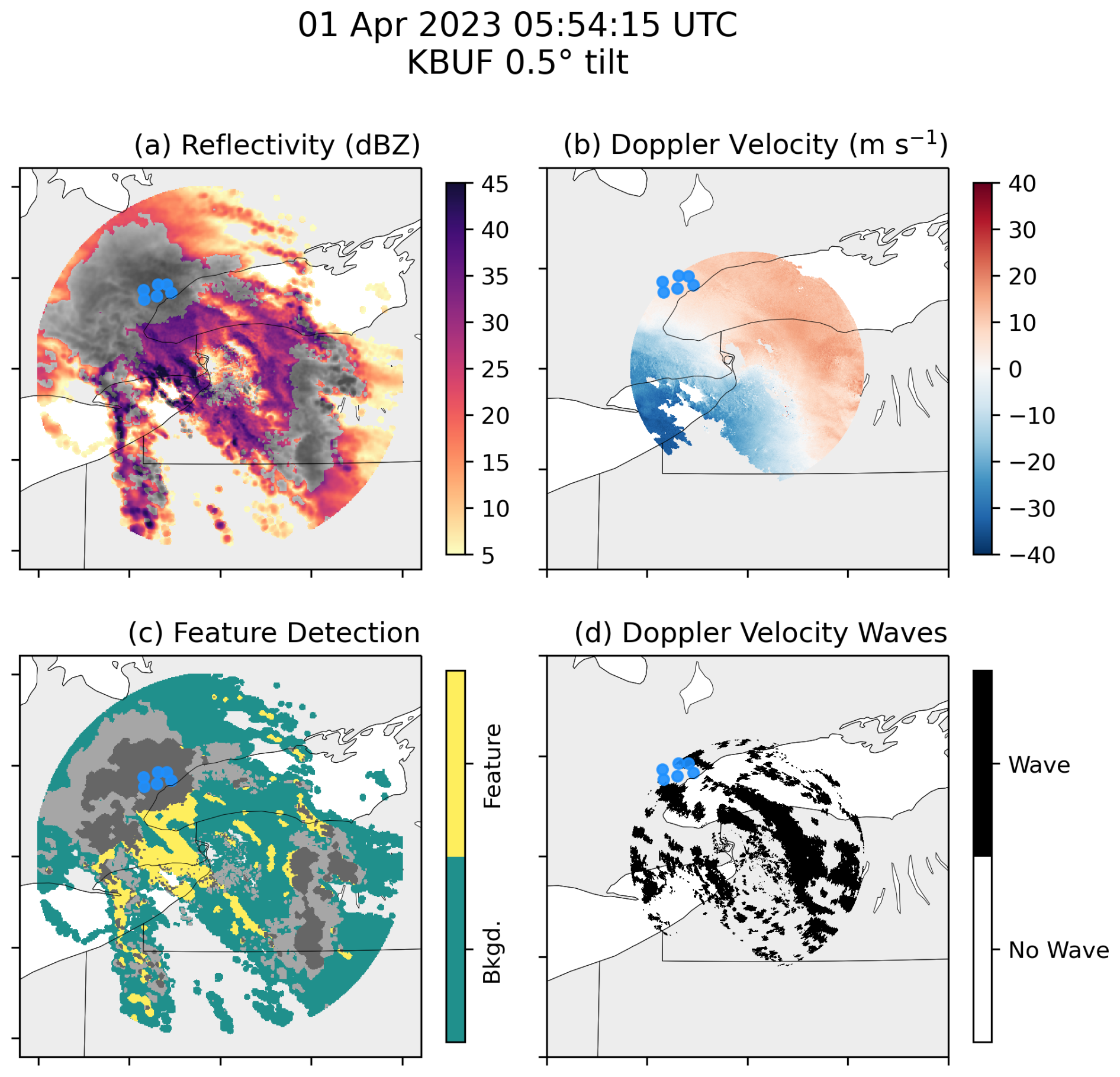
Figure 4 Event-19 (gravity wave event) maps of (a) reflectivity, (b) radial Doppler velocity, (c) detected features of enhanced reflectivity, and (d) Doppler velocity wave detection for KBUF at 05:54 UTC on 1 April 2023. Filled blue circles indicate the locations of pressure sensors in Toronto. In this example, gravity waves moved southwest to northeast, while a northwest–southeast-aligned linear region of enhanced reflectivity about 150 km long and 80 km wide extends from near the western edge of Lake Ontario. Several northwest–southeast-aligned Doppler velocity waves could be tracked from southwest to northeast between Lake Erie and Lake Ontario. The greyscale regions in panels (a) and (c) likely contain mixed precipitation (reflectivity >20 dBZ and a dual-polarization correlation coefficient <0.97). An animated version of this figure is available in the Video supplement (Animation-Figure-S01).

Reflectivity bands were identified as roughly linear features of high reflectivity relative to the background reflectivity, following Tomkins et al. (2024b). To find features of locally enhanced reflectivity, we first calculate the background reflectivity as a windowed average in radii of 20 km. Grid points with a reflectivity sufficiently exceeding that background average, or that have a reflectivity ≥35 dBZ, are identified as features (Fig. 4c). When mapping the reflectivity and detected high-reflectivity features, we “mute” regions with enhanced reflectivity likely due to melting and mixed precipitation (a reflectivity >20 dBZ and a correlation coefficient <0.97) by plotting in greyscale (Fig. 4a and c; Tomkins et al., 2022). In Fig. 4, enhanced reflectivity features were found throughout the coverage of the KBUF radar; however, most notably, there were linear features near the eastern edge of Lake Erie and extending southeastward.

We identified Doppler velocity waves following Miller et al. (2022). We first calculate the difference in radial velocity between successive NWS WSR-88D scans. That difference field is then converted to a binary field; i.e., positive values are converted to zeros, whereas negative values are converted to ones. Small objects are filtered out of the binary field. In Fig. 4d, Doppler velocity waves are detected across the radar domain; however, most notably, the wave extending from west central Lake Ontario eastward then southward into New York State could be tracked as a coherent feature across several radar scans (Animation-Figure-S3.01 in the Video supplement).

We analyzed the resulting sequences of maps for each wave event to determine whether any coherent bands or waves were present anywhere within the range of the radar. Additionally, if any bands or waves were present, we assessed whether they propagated directly over the pressure sensors at a velocity consistent with the estimated phase velocity of the pressure waves.

2.4 Surface stations and operational soundings

We used hourly ASOS data (NOAA National Centers for Environmental Information, 2021a) to assess precipitation type and liquid-water-equivalent precipitation amount during each pressure wave event. We counted the Meteorological Aerodrome Report (METAR) snow precipitation type and snow mixed with other precipitation types as “snow”. We tabulated the total number of hours during our analysis period for which at least a 0.1 mm h⁻¹ of snowfall liquid-water-equivalent rate was measured. For New York, we were able to use data from John F. Kennedy International Airport (KJFK) to obtain both precipitation type and snowfall intensity. As precipitation amounts at Toronto Pearson International Airport (CYYZ) were not available in the archived data, we used precipitation amount data from the Downtown Toronto (CXTO) ASOS, which does not record precipitation type, and precipitation type data from the Toronto City Airport (CYTZ) ASOS, which is closer to CXTO than CYYZ but does not record precipitation amount.

We used 1 min ASOS data to help determine whether each wave event was directly caused by the passage of a front or outflow boundary and its associated density and temperature change (e.g., when a sharp rise in pressure co-occurred with sharp drops in temperature and dew point). We also considered the radar and surface analysis maps when determining whether an event was directly caused by a front or outflow boundary passage. Examples of pressure wave events associated with an outflow boundary passage and a frontal passage, along with contextual data are shown by Allen et al. (2024d) in their Sect. 4.3 and 4.4, respectively. In one case, a pressure wave event was caused by a convective wake low passage, as indicated by the timing of the event relative to a mesoscale convective system passage (Allen et al., 2024d). Ideally, if we saw surface wind perturbations correlated with the pressure perturbations in 1 min ASOS data, it would strongly suggest that the pressure perturbations are associated with gravity waves. However, <1 min surface wind data sets at the locations of the pressure sensor network sensors are not available. ERA5 and other reanalysis are too coarse with respect to their spatial and temporal scales to use for this purpose. We separated the front, outflow boundary, and wake low cases from the remaining cases, which we refer to as gravity wave events.

We analyzed upper-air radiosonde observations for gravity wave events with a nearby NWS weather balloon (Fig. 2) launched during a time window from 2 h before the start of the wave event to 2 h after the end of the wave event. For gravity wave events in the Toronto pressure sensor network, radiosonde data from Buffalo, NY (KBUF), were used, whereas for gravity wave events in the New York and Long Island pressure sensor network, radiosonde data from Upton, NY (KOKX), were used. We obtained the data from IGRA (NOAA National Centers for Environmental Information, 2021b) and interpolated them to a constant 100 m vertical resolution. When sounding data were available, we determined whether an efficient wave duct was present (conditionally unstable layer above an absolutely stable layer; Lindzen and Tung, 1976), as in Fig. 10 in Allen et al. (2024d), which added confidence that the pressure wave event was associated with gravity waves. For each sounding associated with a gravity wave event, we will determine whether a surface-adjacent temperature inversion was present or if any temperature inversions were present in the lowest 1 km above the surface. We identified temperature inversion layers as any observations for which the temperature increased with increasing height.

3 Pressure wave characteristics and environmental context

Table 3 lists the important attributes of all 33 pressure wave events and labels the events (by number) that will be referred to in the following text. No pressure wave events were detected between June and August (Fig. 5a). A total of 5 pressure wave events were solitary waves coincident with frontal passages, 4 pressure wave events were coincident with outflow boundary passages, 1 pressure wave event was caused by a wake low associated with a mesoscale convective system (Allen et al., 2024d), and the other 23 pressure wave events are considered gravity wave events (Fig. 5b and c).

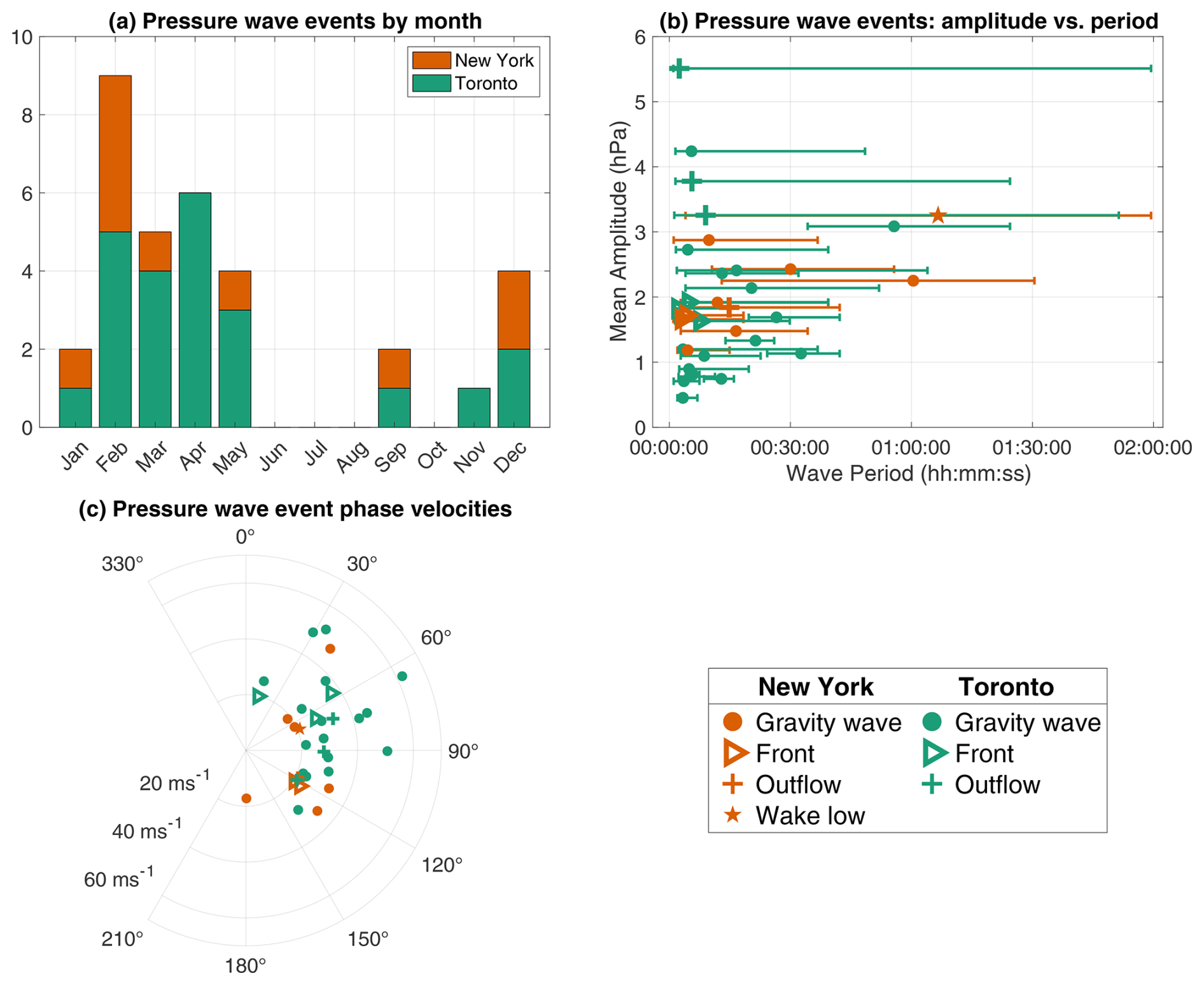
Figure 5 Characteristics of the 33 pressure wave events detected in New York (orange) and Toronto (green) between January 2020 and April 2023. (a) Bar chart of the number of pressure wave events by month. (b) Scatterplot of wave amplitude against wave period, with error bars indicating the range of wave periods for which $W\ge \mathrm{10}\langle \left|W\right(b,a\left)\right|{\rangle }_b$, i.e., where there was a strong wave signal. (c) Radial scatterplot of the wave phase velocities (directions shown are in degrees clockwise from northbound). In panels (b) and (c), gravity wave events are indicated by filled circles, whereas front, outflow, and wake low events are indicated by other shapes according to the legend.

There did not appear to be a strong relationship between wave period and wave amplitude for pressure wave events (Fig. 5b); this is somewhat surprising, given that the mean wavelet power generally increases with wave period for pressure (Canavero and Einaudi, 1987; Grivet-Talocia and Einaudi, 1998; Allen et al., 2024d). Figure 5b includes the range of wave periods for which the wavelet power exceeded A(a) as error bars. From these error bars, it is apparent that nearly every pressure wave event had a strong wave signal at shorter wave periods (<30 min), while very few had a strong wave signal at longer wave periods (>90 min).

Every pressure wave event had an eastward component to its phase velocity (Fig. 5c). This result is similar to Grivet-Talocia et al. (1999), who found that 95 % of pressure wave events in central Illinois had an eastward component to their phase velocities. A total of 19 of the pressure wave events (58 %) that we detected had a northward component to their phase velocities, while 14 pressure wave events (42 %) had a southward component to their phase velocities. A total of 20 out of 33 (61 %) pressure wave events that we detected had a phase speed of between 20 and 35 m s⁻¹, again similar to Grivet-Talocia et al. (1999).

3.1 Gravity wave event characteristics

We will focus on the 23 gravity wave events to address their environmental and radar contexts, with an emphasis on winter storms. All 23 gravity wave events occurred between December and May (Table 3). Figure 6 shows the extracted event and total pressure time series for a single sensor for each of those 23 gravity wave events. Most events consisted of multiple pressure oscillations. In some cases, the amplitudes of those oscillations varied with time (e.g., events 2, 14, and 24), while the oscillations remained at a steady amplitude through the event in other cases (e.g., events 11 and 18). The gravity wave events had a wide range of durations, wave amplitudes, and wavelengths (Fig. 5). The event duration varied over a wide range. Event 5 was a solitary wave of depression with a duration of roughly 1 h. Event 22 had a duration of nearly 20 h.

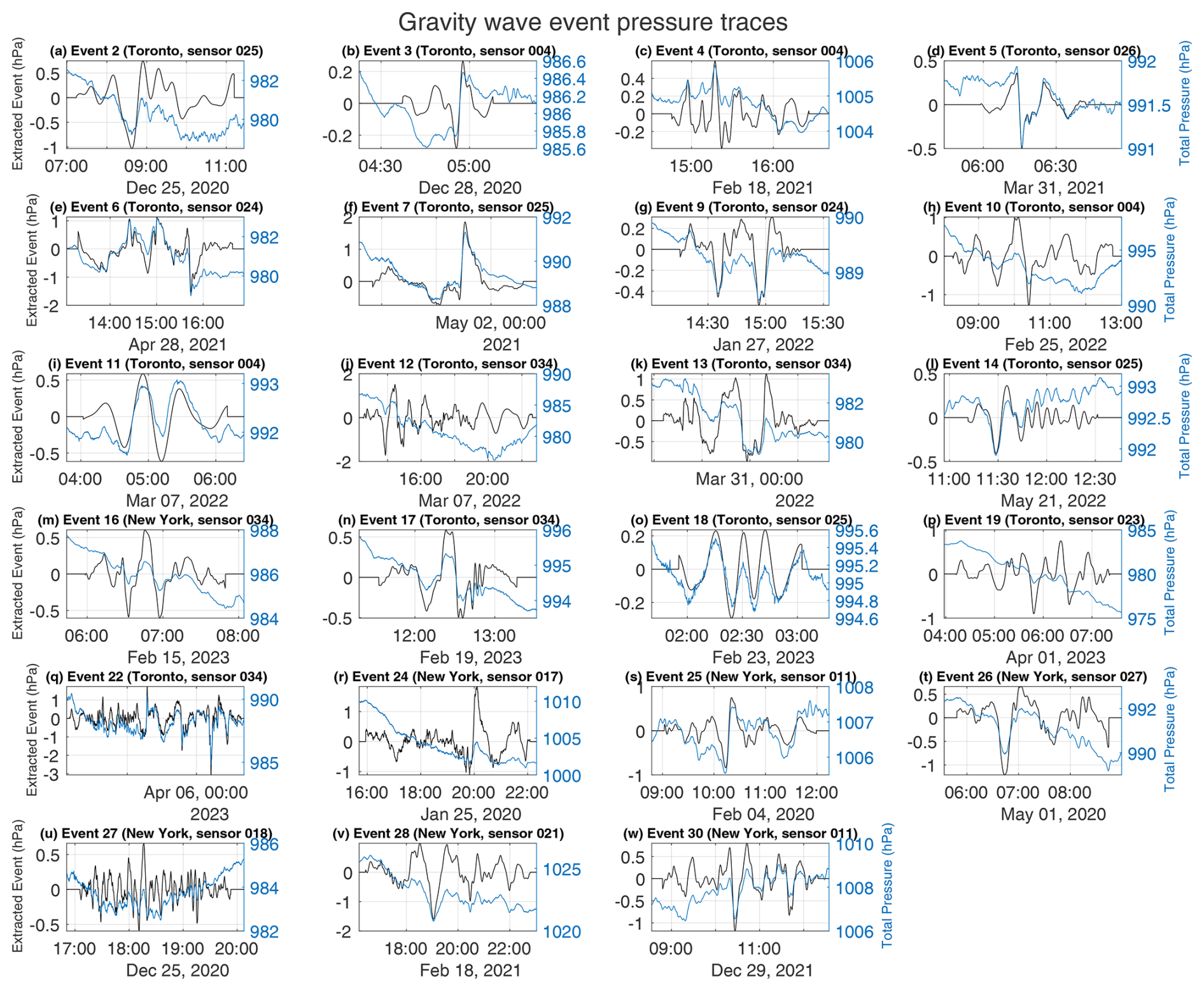
Figure 6 Extracted pressure wave event (black, left axes) and total pressure (blue, right axes) time series for the 23 gravity wave events. The ordering and numbering of wave events matches that in Table 3. For each gravity wave event, data from only a single sensor are shown. That sensor was chosen to maximize its optimal cross-correlation values with extracted event traces from other sensors that captured a given gravity wave event.

For the 23 gravity wave events, a strong linear correlation between wave amplitude and event duration was found (R=0.88, p value = $\mathrm{3.2}\times {\mathrm{10}}^{-\mathrm{8}}$; Fig. 7). A simple linear regression suggests that a 1 hPa increase in amplitude roughly corresponds to a 170 min increase in event duration. It is possible that part of this correlation is due to the event extraction method. Testing on synthetic events with constant duration (not shown) showed that the higher-amplitude waves result in more residual wavelet signal extending beyond the given event duration. Given the large range of event durations over which this correlation holds, there is likely some physical meaning to the relationship. A similar relationship has been documented in seismic waves: higher-magnitude earthquakes tend to have longer durations (e.g., Trifunac and Brady, 1975; Herrmann, 1975), which can be explained by the stronger earthquakes propagating over larger areas of fault surfaces (e.g., Bonilla et al., 1984; Wells and Coppersmith, 1994) and, thus, having larger source areas. This raises the question of whether higher-amplitude gravity waves have larger source areas, which is not possible to adequately answer with the data used in this study.

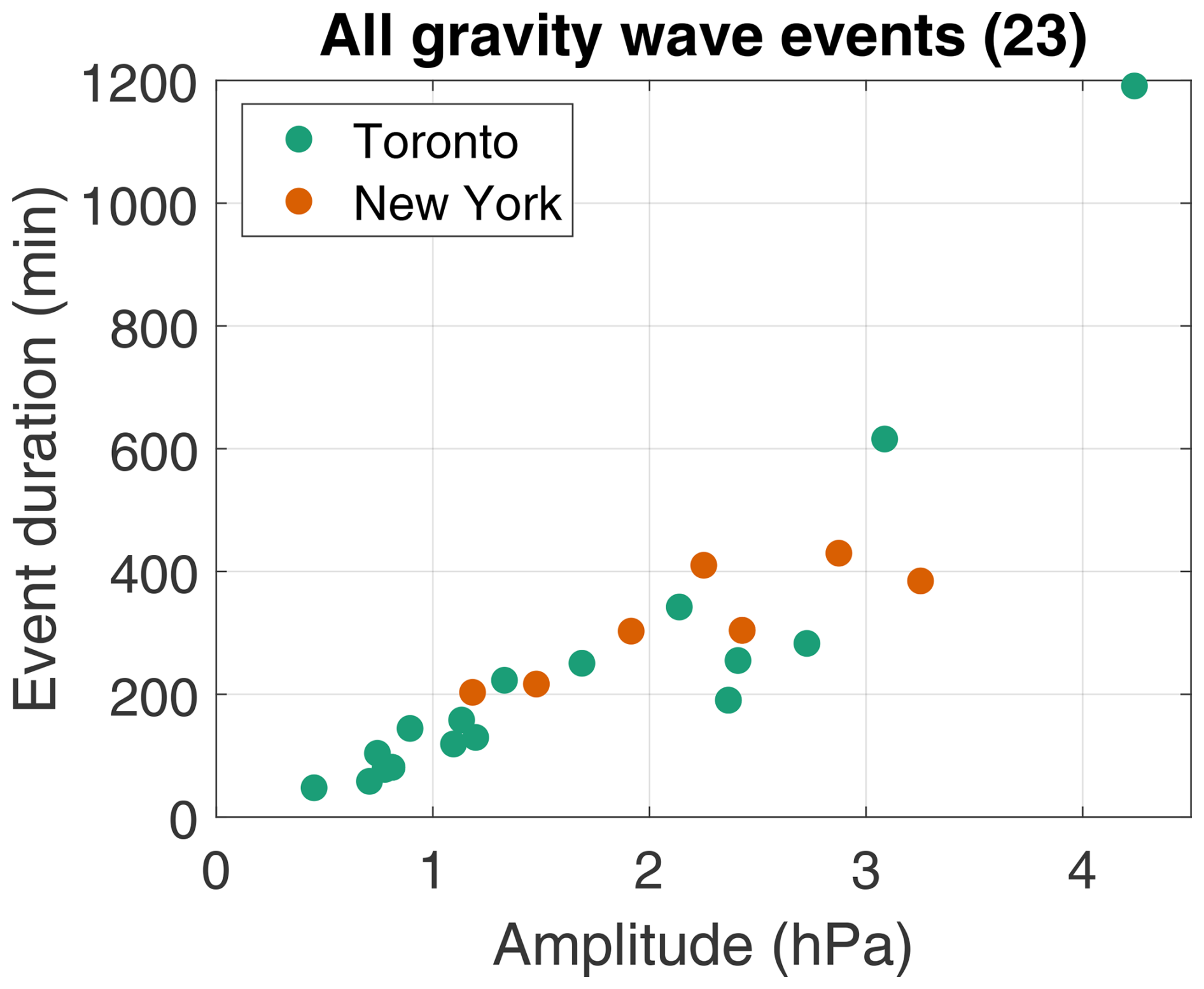
Figure 7 Scatterplot of wave amplitude against event duration for the 23 gravity wave events. Green points represent gravity wave events in Toronto, whereas orange points represent events in New York and Long Island.

3.1.1 Relating pressure perturbations to vertical parcel displacements for gravity waves

To give further context to the pressure perturbations associated with gravity waves, we can compute the vertical parcel perturbation for a case in which representative sounding data are available. The sounding launched at KBUF during event 10 in Toronto on 25 February 2022 is useful for this, as there is a clear gravity wave ducting layer in that example (Fig. 10 in Allen et al., 2024d). Equation (68-3) from Gossard and Hooke (1975) relates the pressure perturbation (P₀ in pascals) to the vertical parcel displacement (ζ_H in meters) for a given gravity wave ducting layer depth (H in meters):

$$\begin{array}{}\text{(11)}& {\mathit{\zeta }}_H={\displaystyle \frac{H}{{\mathit{\rho }}_{\mathrm{s}}(\frac{\mathit{\omega }}{k}{)}^{\mathrm{2}}}}B{P}_{\mathrm{0}},\end{array}$$

where ρ_s is the surface air density (1.225 kg m⁻³ for this example), ω is the intrinsic angular wave frequency (in s⁻¹), and k is the horizontal wavenumber (in m⁻¹). ω and k are calculated as follows:

$$\begin{array}{}\text{(12)}& {\displaystyle }\mathit{\omega }={\displaystyle \frac{\mathrm{2}\mathit{\pi }}{\mathit{\tau }}}-u_{\mathrm{0}}k,\text{(13)}& {\displaystyle }k={\displaystyle \frac{\mathrm{2}\mathit{\pi }}{\mathit{\lambda }}},\end{array}$$

where τ is the wave period (1222 s for this example; Table 3), u₀ is the mean wind speed within the wave duct (18.9 m s⁻¹ for this example), and λ is the wavelength (55.5 km for this example; Table 3). For this example, ω=0.003 s⁻¹ and k=0.11 km⁻¹. The calculation of B depends on the Brunt–Väisälä frequency (N in s⁻¹). The wave duct is saturated for this example (Fig. 10 in Allen et al., 2024d), so we calculate the moist Brunt–Väisälä frequency N_m (Markowski and Richardson, 2010, p. 42):

$$\begin{array}{}\text{(14)}& N_{\mathrm{m}}=\sqrt{{\displaystyle \frac{g}{{\mathit{\theta }}_{\text{e0}}}}{\displaystyle \frac{{\mathrm{\Gamma }}_{\mathrm{m}}}{{\mathrm{\Gamma }}_{\mathrm{d}}}}{\displaystyle \frac{\partial {\mathit{\theta }}_{\mathrm{e}}}{\partial z}}},\end{array}$$

where g is the gravitational acceleration (∼9.81 m s⁻²), θ_e0 is the mean equivalent potential temperature in the wave duct (294.7 K for this example), Γ_m is the moist adiabatic lapse rate in the wave duct (7.58 K km⁻¹ for this example), Γ_d is the dry adiabatic lapse rate (9.76 K km⁻¹), and $\frac{\partial {\mathit{\theta }}_{\mathrm{e}}}{\partial z}$ is the change in equivalent potential temperature with height in the wave duct (20.2 K km⁻¹ for this example). For this example, N_m=0.023 s⁻¹. We also need the vertical wavenumber n₁ (in m⁻¹) to calculate B. n₁ is calculated as follows:

$$\begin{array}{}\text{(15)}& n_{\mathrm{1}}=k\sqrt{{{\displaystyle \frac{N_{\mathrm{m}}}{\mathit{\omega }}}}^{\mathrm{2}}-\mathrm{1}}.\end{array}$$

For this example, n₁=0.853 km⁻¹. As ω<N_m, B is calculated as follows (Gossard and Hooke, 1975):

$$\begin{array}{}\text{(16)}& B={\displaystyle \frac{\sin \left(n_{\mathrm{1}}H\right)}{n_{\mathrm{1}}H}}.\end{array}$$

For this example, B=0.656. Finally, the peak-to-trough amplitude of the gravity wave was ∼2 hPa for event 10 (Table 3); therefore, we take half of that, 1 hPa, as the pressure perturbation P₀, so the vertical parcel displacement ζ_H=129 m for this example. This result is of a similar order of magnitude to the vertical displacements reported by Kjelaas et al. (1974) (50–120 m) and Allen et al. (2013) (400 m).

3.1.2 Synoptic context for gravity wave events

The synoptic environmental context for each of the 23 gravity wave events that occurred during our 40 months of analysis (Table 4) permits comparisons to previous case studies and theoretical work. For each gravity wave event, we examined surface pressure and equivalent potential temperature (Fig. 8), 300 hPa geopotential heights and wind speeds (Fig. 9), and 300 hPa ΔNBE (Fig. 10). For a gravity wave to be detected at the surface, there needs to be suitable conditions for the wave signal to reach the surface (e.g., there should ideally be no convective overturning in the boundary layer which would obscure the pressure signal due to the gravity wave).

Table 4 Environmental context for the 23 gravity wave events detected over the 40-month analysis period. The leftmost column is an index column, aligned with the index column in Table 3. Here, the position of wave events relative to the low and to air mass boundaries was determined based on manual analysis of θ_e and MSLP maps derived from ERA5 data at the center time of the event (Fig. 8). If no air mass boundary could be discerned near Toronto or New York for an event, we consider it “Unclear” whether that event occurred in the cold sector or warm sector. Events 25 and 30 occurred roughly 2000 km or more to the east of the nearest cyclone, as indicated in the table and the text.

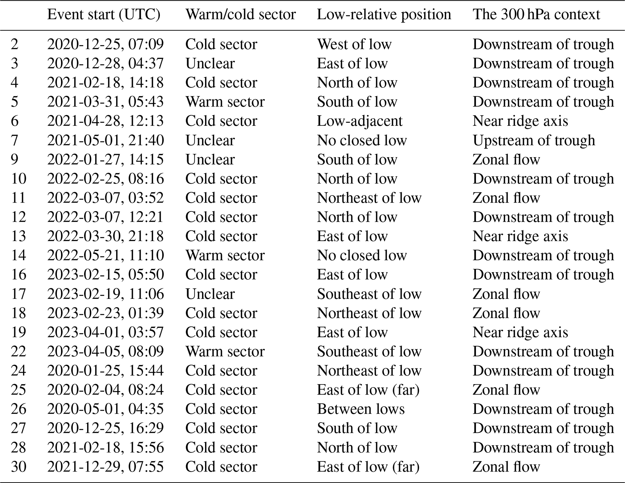
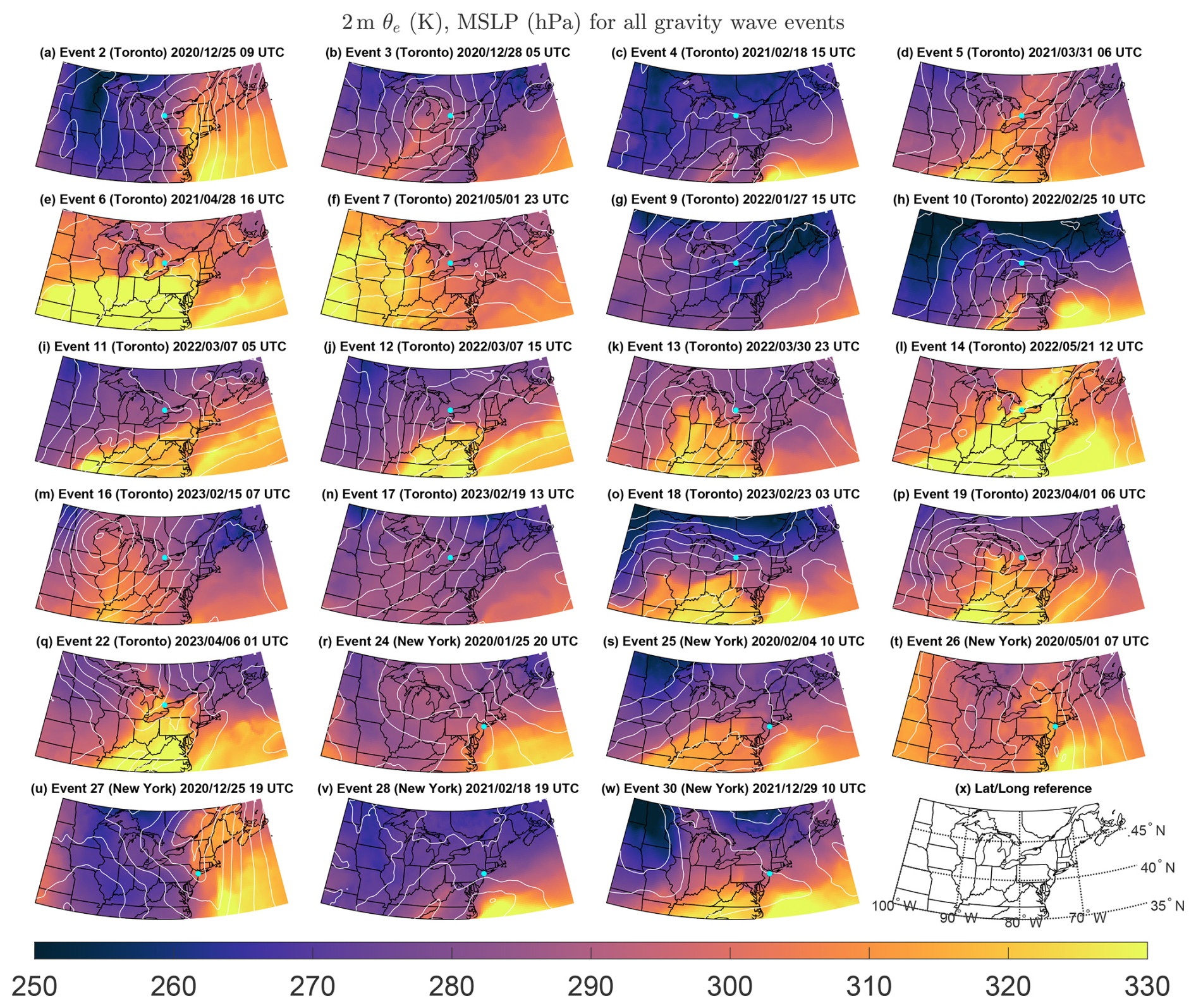
Figure 8 (a–w) The ERA5 2 m equivalent potential temperature maps for all of the detected gravity wave events, at the center time of each event. The ordering and numbering of events matches that in Table 3. MSLP is contoured in white every 5 hPa. In each panel, either New York or Toronto is shown by a cyan point, depending on where the gravity wave event occurred. (x) Latitude and longitude reference map.

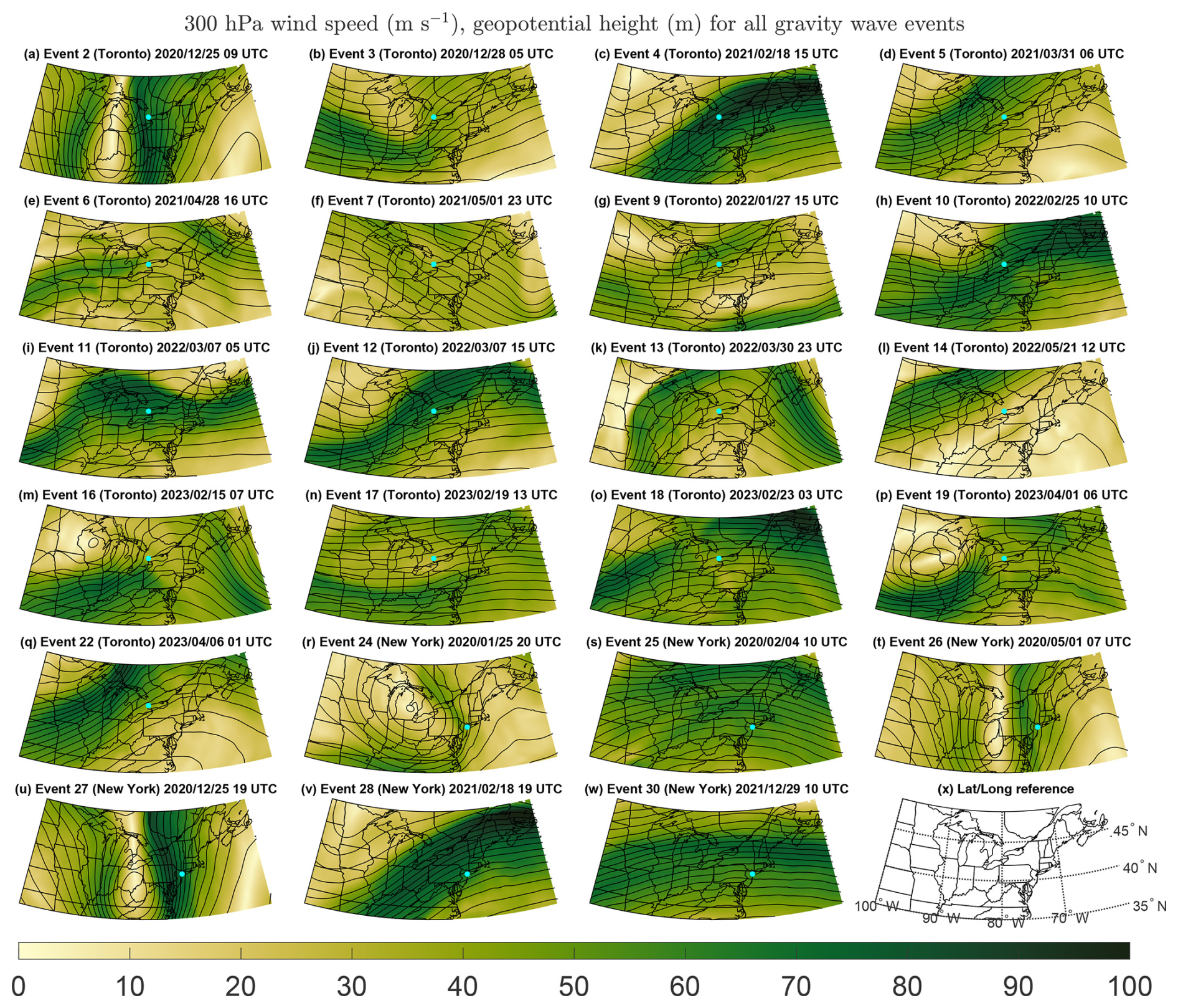
Figure 9 (a–w) The ERA5 300 hPa wind speed maps for all of the detected gravity wave events, at the center time of each event. The ordering and numbering of events matches that in Table 3. The 300 hPa geopotential height is contoured in black every 50 m. In each panel, either New York or Toronto is shown by a cyan point, depending on where the gravity wave event occurred. (x) Latitude and longitude reference map.

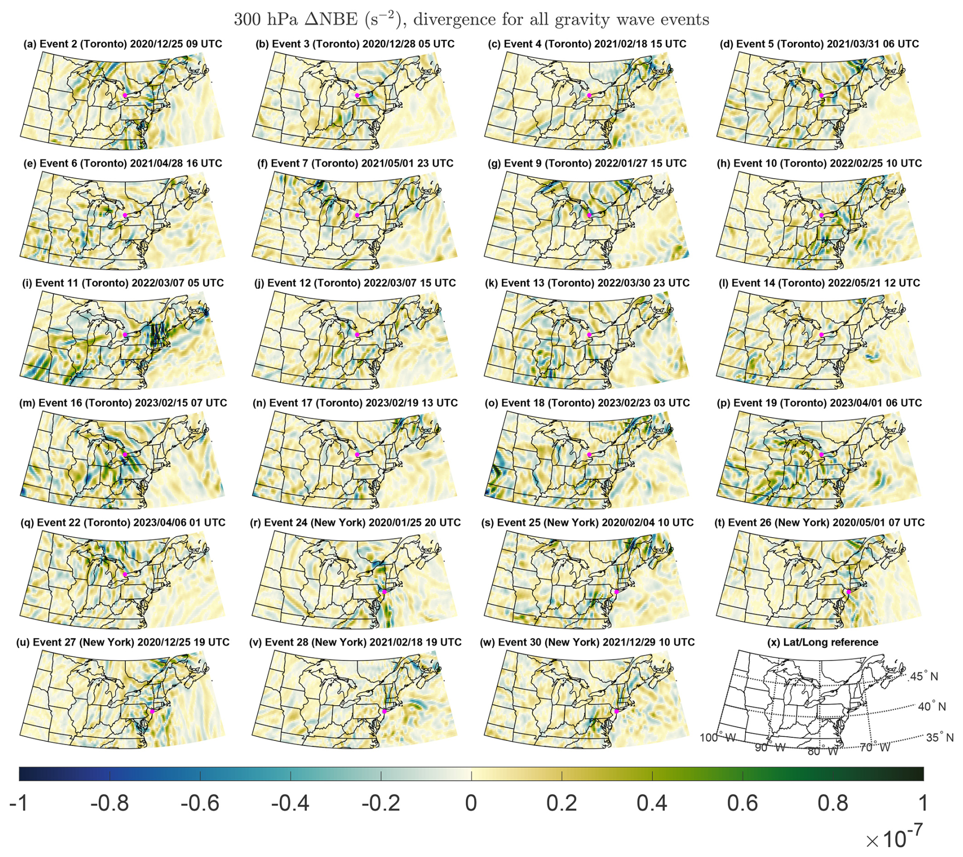
Figure 10 (a–w) The ERA5 300 hPa ΔNBE maps for all of the detected gravity wave events, at the center time of each event. The ordering and numbering of events matches that in Table 3. In each panel, either New York or Toronto is shown by a cyan point, depending on where the gravity wave event occurred. (x) Latitude and longitude reference map.

Previous studies (e.g., Uccellini and Koch, 1987; Koch and Golus, 1988) have often found mesoscale gravity waves east of surface lows and downstream of upper-level troughs. Our analysis of the 23 gravity wave events in the Toronto and New York metropolitan areas between January 2020 and April 2023 largely agrees with those findings. In such cases, gravity waves may have been triggered by the balance adjustment mechanism described by Zhang et al. (2001). The gravity wave events associated with 300 hPa zonal flow with weak or no flow imbalance in the region were likely related to different mechanisms, such as localized latent heating or interactions between waves propagating from farther afield (Fritts and Alexander, 2003). With the available observations and reanalysis data, it is not possible to determine the gravity wave trigger mechanism with complete certainty.

Surface low center cyclone tracks for storms that produce snowfall in the northeastern US are most common near the coast and over the Atlantic Ocean, to the east of New York City and Toronto (Fig. 11). Of the 23 gravity wave events in Toronto and New York during our 40-month analysis period, 15 (65 %) occurred north or east of a surface low (events 3, 4, 10, 11, 12, 13, 16, 17, 18, 19, 22, 24, 25, 28, and 30), often on the cool side of warm or stationary fronts. This includes events 25 and 30, which were more than 2000 km away from the low. Event 22 had such a long duration that it began when Toronto was on the cool side of a warm front and ended after the warm front had passed. Event 2 occurred behind a cold front and to the west of a surface low. Events 5, 9, and 27 occurred south of lows. The remaining cases are more complex. Event 6 occurred near a weak surface low and just on the cool side of an air mass boundary. Event 26 occurred near a weak air mass boundary with lows both to the north and the south. Events 7 and 14 occurred with no closed low in the region (Fig. 8).

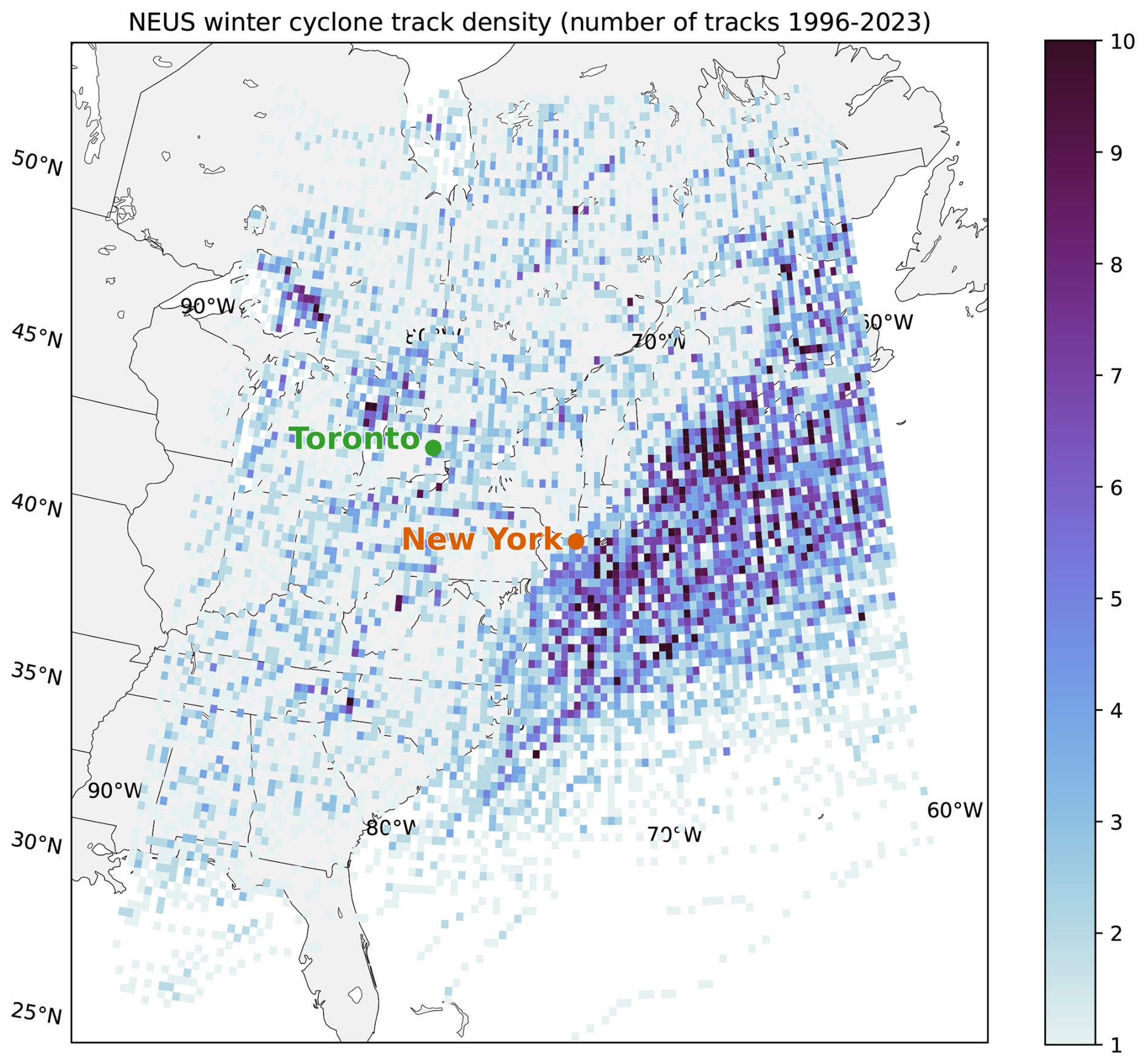
Figure 11 Cyclone track density (shading) for storms in the northeastern US (NEUS) which brought at least 1 in. (∼ 25.4 mm) of snowfall in a 24 h period to at least two ASOS stations in the NEUS between 1996 and 2023. Cyclones were tracked using ERA5 data following the methodology of Crawford et al. (2021).

Inversion layers at altitudes <1 km were found in all of the 12 gravity wave events when upper-air soundings were launched either during or within 2 h of the events (Fig. 12). Event 22 had two radiosonde launches. Many of the inversion layers were only 100–200 m deep. Events 6, 17, 22, and 25 had an inversion layer adjacent to the surface. A near-surface stable layer likely helps to maintain the coherence of the gravity wave signal across the network of sensors (Uccellini and Koch, 1987). Coincident upper-air soundings were not available for events 7 and 14, during which gravity waves occurred with no closed surface low anywhere in the domain that we analyzed (Fig. 8).

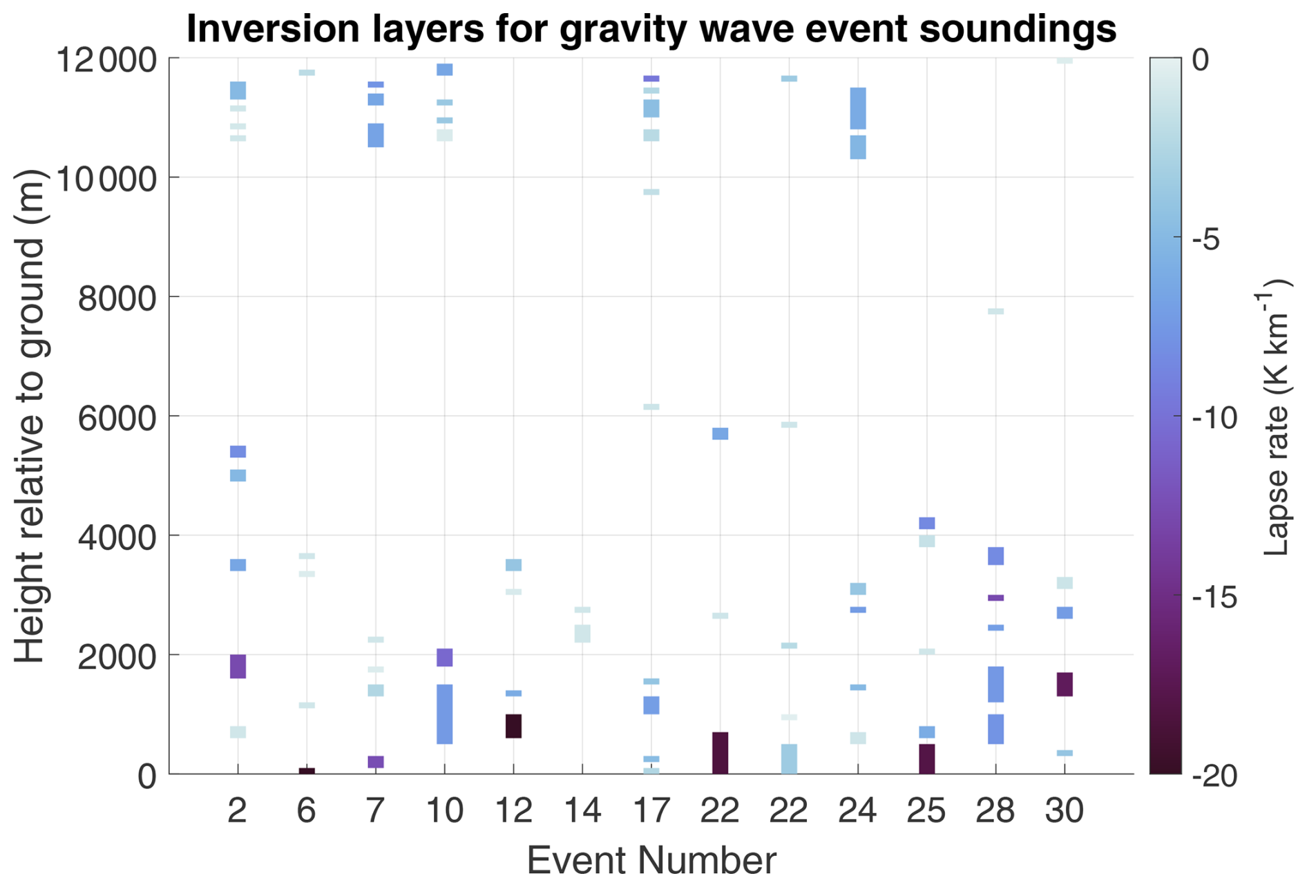
Figure 12 Air temperature inversion layers for soundings launched at KBUF, for gravity wave events in Toronto, or at KOKX, for gravity wave events in New York and Long Island, either during or within 2 h of a gravity wave event. Inversion layers are colored according to the layer-average lapse rate (darker colors indicate a stronger inversion). Event numbering matches that in Table 3. Two soundings were launched at KBUF during event 22. Events 2–22 were in Toronto, whereas events 24–30 were in NY.

In terms of the large-scale synoptic pattern aloft, 13 gravity wave events occurred downstream of 300 hPa troughs and upstream of 300 hPa ridges (events 2, 3, 4, 5, 10, 12, 14, 16, 22, 24, 26, 27, and 28; Fig. 9, Table 4), consistent with most gravity wave events shown by Uccellini and Koch (1987). Six other events occurred in roughly zonal 300 hPa flow regimes (events 9, 11, 17, 18, 25, and 30), and three gravity wave events occurred below a 300 hPa ridge (events 6, 13, 19). One gravity wave event occurred upstream of a 300 hPa trough (event 7).

Regions with large-magnitude ΔNBE, regardless of sign, imply flow imbalance and the possibility of resulting gravity wave genesis. If gravity waves are triggered by flow imbalance at 300 hPa, they would not necessarily be observed on the ground directly beneath the trigger area, as the wave signal must reach the lower troposphere to be observed, which might require the waves to propagate some distance vertically and horizontally. A total of 18 of the 23 gravity wave events occurred with large 300 hPa flow imbalance to the south or west (events 2, 3, 5, 6, 7, 9, 10, 11, 13, 14, 16, 18, 19, 22, 24, 25, 27, and 30; Fig. 10). Considering that many of the gravity wave events were observed to propagate from west to east (Fig. 5c and Table 3), it is plausible that many were triggered by flow imbalance aloft.

3.1.3 Radar echo and precipitation type context for gravity waves

NWS WSR-88D radar echo corresponds to precipitation-sized particles in the resolution volume. Only within regions with radar echo can enhanced reflectivity features and Doppler velocity waves be detected. Table 5 shows the radar echo characteristics and ASOS precipitation type context for each gravity wave event.

Table 5 Radar and precipitation context for the 23 gravity wave events detected during our 40-month analysis period. The leftmost column is an index column, aligned with the index column in Table 3. The presence of surface snow was determined using the nearest available ASOS data (CYYZ or KJFK). Echo, reflectivity bands, and Doppler velocity waves are considered “present” when they exist anywhere within the range of the 0.5° scan for the nearest NEXRAD radar (KBUF or KOKX). Reflectivity bands and Doppler velocity waves are considered “co-located” when they are located directly above pressure sensors and their movement is consistent with the gravity wave phase velocity.

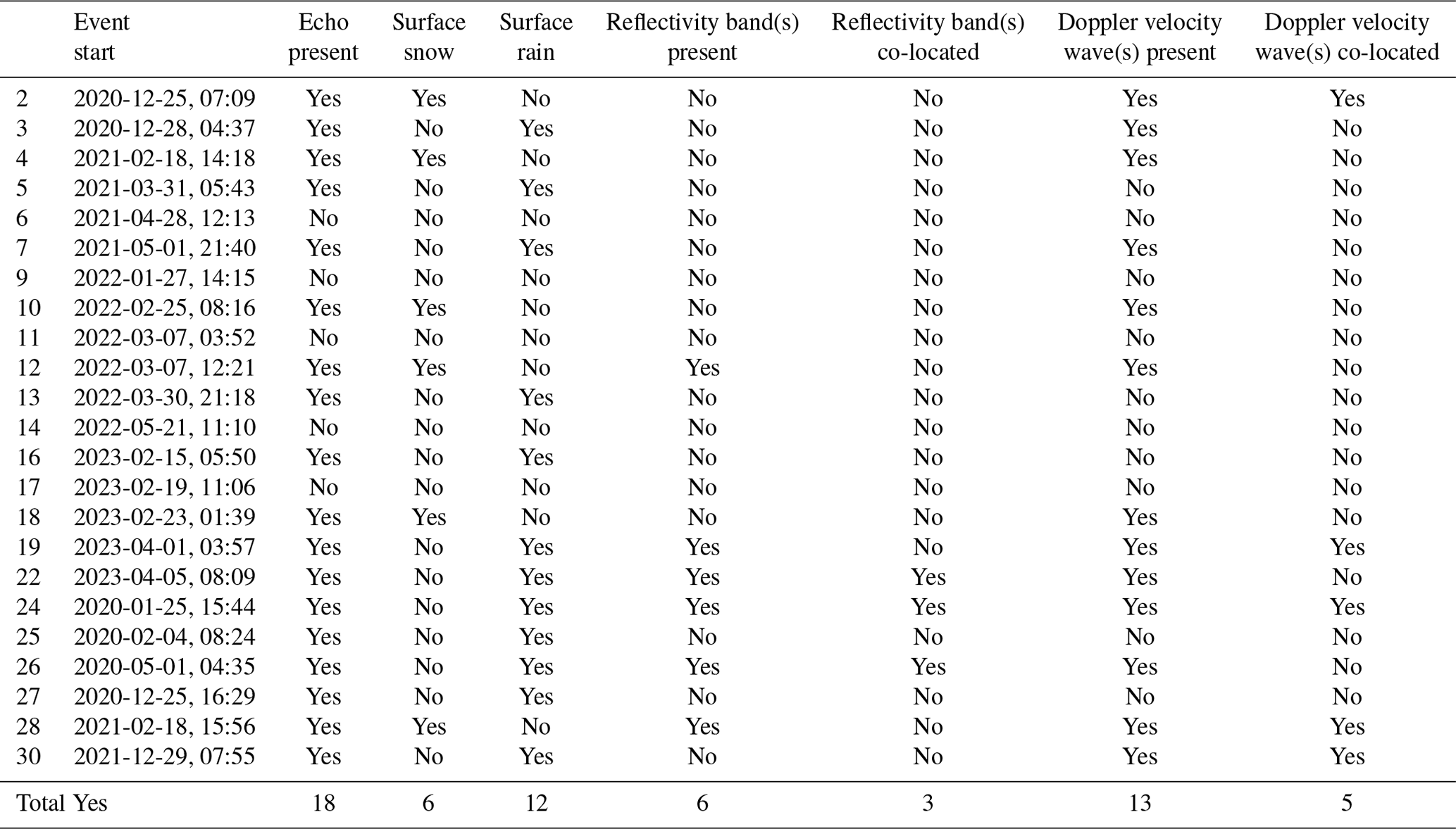
A total of 18 (78 %) of the 23 gravity wave events occurred with precipitation radar echo detected by the nearby WSR-88D in the 0.5° tilt. Only six of these cases (events 2, 4, 10, 12, 18, and 28) co-occurred with surface snow or mixtures including snow. Two of those cases with snow occurred with enhanced reflectivity bands within the radar range, but the movement of the enhanced reflectivity bands was not consistent with the gravity wave phase velocity vector in either case. For example, radar data during event 28 indicate that there was an enhanced reflectivity feature passing over the pressure sensors, but the movement of the enhanced reflectivity feature (southwest to northeast) was not consistent with the phase direction of the gravity waves (northwest to southeast; Fig. 13, Animation-Figure-S3.02 in the Video supplement).

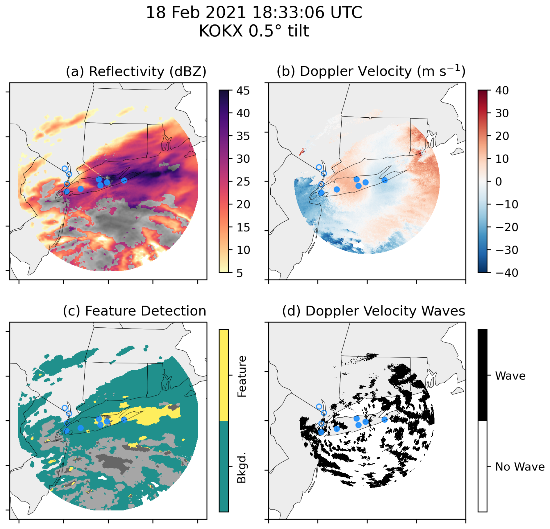
Figure 13 As in Fig. 4 but for KOKX at 18:30 UTC on 18 February 2021, during event 28 (gravity wave event). In this example, an elongated enhanced reflectivity feature passed over the pressure sensor network from southwest to northeast during the wave event, which was inconsistent with the gravity wave phase direction (northwest to southeast). An animated version of this figure is available in the Video supplement (Animation-Figure-S02).

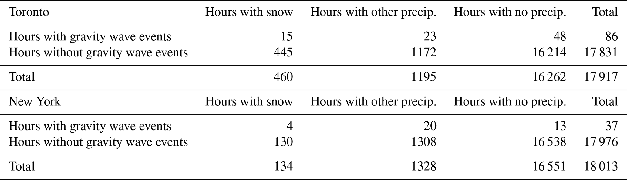
Overall, gravity waves during surface snow were rare at our locations. Periods of snowfall at a rate of at least 0.1 mm h⁻¹ (liquid equivalent) for at least 4 h, with at most a 1 h gap without that rate of snowfall, occurred 59 times in Toronto and 20 times in New York during our analysis period. A total of 51 of those 59 snow storms in Toronto and a total of 16 of the 20 snow storms in New York occurred between November and February, mostly before the peak in gravity wave events (February–May; Fig. 5a). In the Toronto area, there were 460 h with at least 0.1 mm h⁻¹ (liquid equivalent) of snow recorded. Of this time, only 15 h with snow was during a gravity wave event. In the New York area, snow was recorded for 134 h, of which only 4 h occurred during gravity wave events (Table 6). It had been surmised that gravity waves may often be associated with groups of enhanced reflectivity bands in snow (multibands; Hoban, 2016), but we did not find enough gravity wave events on the typical spatiotemporal scales of multibands during snowfall events over our analysis period to support that notion.

Table 6 Hours with and without gravity wave events subdivided by ASOS precipitation data during the November to May months between January 2020 and April 2023. Precipitation (precip.) was determined to be present when there was ≥0.1 mm h⁻¹ liquid-equivalent precipitation recorded at Toronto (CYTZ precipitation type and CXTO precipitation amount) and at New York (KJFK precipitation type and amount). Hours with either only snow or a mixture of precipitation types containing snow are included under hours with snow.

When surface rain was present, three gravity wave cases (events 22, 24, and 26) had enhanced reflectivity features co-located and moving at a velocity consistent with the pressure waves. During event 22, an elongated reflectivity feature crossed the pressure sensor network and appeared to move at a velocity consistent with the gravity wave phase velocity (Fig. 14, Animation-Figure-S3.03 in the Video supplement). The reflectivity band was an isolated feature lasting only 2 h during a wave event that lasted nearly 20 h. Event 24 occurred along with an occluded front that passed over the pressure sensor network at 20:00 UTC on 25 January 2020. We chose to categorize event 24 as a gravity wave rather than a “front” event because of the pressure oscillations observed in the hours before the occluded front passage (Fig. 6). During event 26, a narrow region of enhanced reflectivity on the trailing edge of a broader precipitation region passed over the pressure sensors in New York near the same time as a large pressure minimum (06:45 UTC on 1 May 2020; Fig. 6).

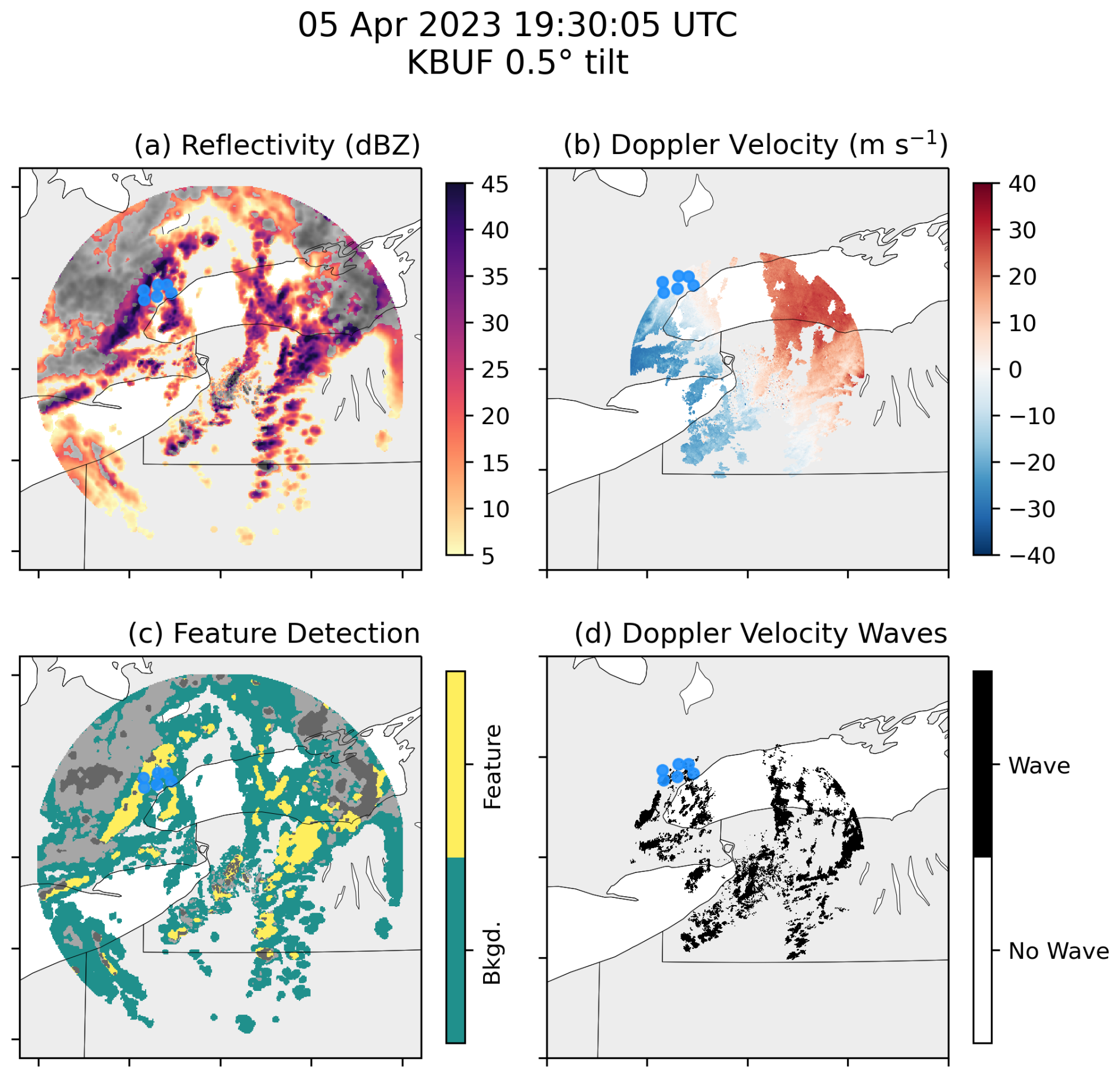
Figure 14 As in Fig. 4 but for KBUF at 19:30 UTC on 5 April 2023 during event 22 (gravity wave event). In this example, gravity waves moved from northwest to southeast while an elongated enhanced reflectivity feature was passing over the pressure sensors in Toronto from west to east. An animated version of this figure is available in the Video supplement (Animation-Figure-S03).

Depending on the spatial scale of gravity waves and the height and depth of the wave duct as well as their 3D position relative to the slanting WSR-88D scans, the transient convergence and divergence signals associated with the gravity waves' propagating upward and downward motions may or may not yield radar-detectable Doppler velocity waves. Hence, we do not expect a 1:1 correspondence between detected gravity waves and detected Doppler velocity waves in the 0.5° elevation angle scan.

A total of 13 gravity wave events of the 18 gravity waves with radar echo occurred with coherently moving Doppler velocity waves present anywhere within the range of the nearby WSR-88D radar. However, only five of these had Doppler velocity waves over the pressure sensors moving at a velocity consistent with the gravity wave phase velocity (Table 5). Based on this limited evidence, a subset of gravity waves may manifest a Doppler velocity wave signature. Figure 3 and Eq. (2) from Allen et al. (2024d) suggest that any gravity wave which produces a pressure perturbation ≥0.5 hPa should also produce a detectable velocity wave signal. The velocity waves may not appear in radar Doppler velocity data either because (1) they are above or below the height of the radar beam or (2) there is strong turbulence that obscures the signal associated with gravity waves. In Toronto, the KBUF radar beam is at a higher altitude compared with the KOKX radar beam over New York, and three of the five gravity wave events with corresponding Doppler velocity waves occurred in the New York pressure sensor network.

The Doppler velocity wave detection works best for waves that propagate less than half of their wavelength between successive radar scans (Miller et al., 2022), i.e., which have a wave period at least twice as long as the time between successive radar scans. Typical NEXRAD volume coverage patterns have a ∼4–8 min time between 0.5° elevation scans, and 12 of the 18 gravity wave events that co-occurred with radar echo had a wave period of 999 s or less. Only 2 of those 12 gravity wave events were co-located with Doppler velocity waves that propagated at a velocity consistent with the gravity wave phase velocity. Of the six gravity wave events with a wave period longer than 999 s that co-occurred with radar echo, three were co-located with Doppler velocity waves that propagated at a velocity consistent with the gravity wave phase velocity.

4 Conclusions

We deployed two air pressure sensor networks, one in Toronto (ON, Canada) and the other in the New York City area and Long Island (NY, USA) to study atmospheric gravity waves. In over 3 years of data, we objectively identified 33 pressure wave events that were observed by at least four pressure sensors and for which there was reasonable confidence in the estimate of the wave phase velocities. Our study examined wave amplitudes on the order of 0.5–5 hPa and wave periods on the order of 2–67 min. These spatial and temporal scales were chosen to align with the spatial and temporal scales of radar-observed enhanced reflectivity bands and Doppler velocity waves, both of which were surmised to potentially be related to gravity waves (Hoban, 2016; Miller et al., 2022).

A few of our detected pressure wave events were associated with frontal passages (5), outflows (4), and a wake low (1), and the remaining 23 events were gravity waves, 20 of which occurred in the cool season between November and April. For context, there were 20 snow storms in New York City and 59 in the Toronto metropolitan area over our 40-month observation period. While limited, the observational evidence that we have suggests the lack of a common association between reflectivity bands and gravity waves. Just six of the gravity wave events co-occurred with any surface snowfall (including trace amounts). Only two of those six events had any enhanced reflectivity bands in the vicinity. The spatial wavelengths of the gravity waves and enhanced reflectivity bands were similar; however, in all the cases with snow, the reflectivity bands were either not directly over the pressure sensors or not moving at a velocity consistent with the pressure waves (Table 5). Including events with both rain and snow over the pressure sensor networks, only 5 of 18 gravity wave events also had Doppler velocity waves moving at a velocity consistent with the gravity wave phase velocity. This evidence suggests that most low-level velocity waves are not gravity waves.

Most of the observed gravity wave events were associated with strong upper-level flow imbalance to the south or west of their location, suggesting that the mechanism of balance adjustment described by Zhang (2004) and Ruppert et al. (2022) may be relevant. The occurrence of several gravity waves downstream of an upper-level trough, on the cool side of air mass boundaries, and with a temperature inversion in the lowest 1 km above ground level is consistent with the findings of Uccellini and Koch (1987). However, we cannot confirm that cause of gravity wave genesis with the observational and reanalysis output data that we used.

We found a strong linear relationship between amplitude and event duration for the 23 atmospheric gravity wave events detected (Fig. 7). A potential explanation could be that parcels in gravity waves triggered by a larger initial perturbation might oscillate for a longer time before returning to an equilibrium state. Further exploration of the relationship between gravity wave amplitude and duration is a topic for future research. There may be an analogy to seismic waves in that higher-amplitude earthquakes tend to have longer durations because of the larger rupture area along the fault (Trifunac and Brady, 1975; Herrmann, 1975).

Satellite images of northeastern US winter storms often show undulations in the overlying cirrus. These undulations may be either Kelvin–Helmholtz waves or gravity waves. Kelvin–Helmholtz waves on horizontal scales of ∼3 km could locally alter the cloud microphysical properties (Houser and Bluestein, 2011). The surface pressure should reflect changes throughout the column of air, including gravity waves aloft. However, it is possible that gravity waves in the upper cloud layers with periods of between 3 and 67 min do occur but have their surface pressure signals obfuscated by other perturbations. For example, if there is an unstable layer below the layer with the gravity waves, the pressure wave amplitude at the surface would be reduced and obfuscated by pressure perturbations due to convective overturning (Kjelaas et al., 1974). Wind profiler data would help to resolve whether conditions for Kelvin–Helmholtz waves are present within the cirrus layer.

For the New York City area in particular, the low frequency of occurrence of gravity waves in winter storms is influenced in part by a sample bias related to the typical position of low-pressure centers offshore. The New York City metropolitan area and Long Island are usually in the northwest quadrant of the storm, where gravity waves are not often found (Fig. 11). In both Toronto and New York, most snow storms ≥4 h in duration occurred between December and February, while most gravity waves were detected between February and May (Fig. 5a).

Whereas previous case study work has examined heavy-snow events that had gravity waves, we cast a broad net by putting out pressure sensor networks for an extended time period to see what we could “catch”. Some of the previously studied winter storm gravity wave cases (e.g., Bosart et al., 1998) are clearly not representative of typical winter storms in the northeastern US, as only 6 of the 79 winter storms with snow that occurred over our 40 months of observations had detectable gravity waves. It is well established that gravity waves can locally increase precipitation (e.g., Bosart et al., 1998; Gaffin et al., 2003; Colle, 2004; Allen et al., 2013; Kingsmill et al., 2016). However, if gravity waves of a sufficient amplitude do not occur, they are irrelevant to locally increasing snow rates. Our findings suggest that gravity waves with an amplitude ≥0.5 hPa are much less common in winter storms than reflectivity features on similar spatial and temporal scales, which are present in most winter storms (Hoban, 2016; Ganetis et al., 2018).