A novel identification method for stratospheric gravity waves in nadir viewing satellite observations

Atmospheric gravity waves (GWs) are an important mechanism for vertical transport of energy and momentum through the atmosphere. Their impacts are apparent at all scales, including aviation, weather, and climate. Identifying stratospheric GWs from satellite observations is challenging due to instrument noise and effects of weather processes, but they can be observed from nadir sounders such as the AIRS instrument onboard Aqua. Here, a new method (hereafter “neighbourhood method”) to detect GW information is presented and applied to AIRS data. This uses a variant of the 3D S-transform to calculate the horizontal wavenumbers of temperature perturbations, then find areas of spatially constant horizontal wavenumbers (assumed to be GWs), which allow for creating a binary wave-presence mask. We describe the concept of the neighbourhood method and use it to investigate GW amplitudes, zonal pseudomomentum fluxes, and vertical wavelengths over 5 years of AIRS data. We compare these results to those calculated from GWs detected using another widely used method based on an amplitude cutoff. 35 % of regions of wave activity detected using the neighbourhood method have amplitudes lower than is visible using the amplitude cutoff method. Three regions are studied in greater depth: the Rocky Mountains, North Africa, and New Zealand/Tasmania. GWs detected using the neighbourhood method have wave phase propagation angles consistent with linear theory. Using the neighbourhood method produces new statistics for regional and global GW studies, which compare favourably to the amplitude cutoff GW detection method.

1 Introduction

Atmospheric gravity waves (hereafter referred to as “GWs”) are a vital component in the dynamics of the atmosphere. They are one of the main processes by which energy and momentum are transferred vertically through the atmosphere (Holton, 1982), and as such can have large impacts on aviation, atmospheric chemistry, the general circulation, and other atmospheric phenomena (Olafsson and Agústsson, 2009; Gardner, 2024; Garfinkel and Oman, 2018; Smith et al., 2005). GWs propagate throughout the atmosphere, but have their largest effects at higher altitudes, as according to linear theory, conservation of energy and the exponential drop in density enforce their amplitudes to grow exponentially with height. They are generated by a wide array of mechanisms, such as flow over orography and deep convection (Tsuda et al., 1994; Dörnbrack et al., 2002; Fritts and Alexander, 2003; Achatz et al., 2024). Other mechanisms include geostrophic adjustments from jet streams (Fritts and Luo, 1992), frontal systems (Plougonven and Teitelbaum, 2003; Zhang, 2004), and non-linear wave-wave interactions (Schlutow and Voelker, 2020).

These diverse mechanisms can lead to large differences in the wave properties, with the vast majority of GWs having horizontal wavelengths in the range of a few kilometres up to thousands of kilometres (Choi et al., 2012; Kalisch et al., 2016; Trinh, 2016; Hájková and Šácha, 2023), and periods from minutes to days (Dunkerton, 1982; Baldwin et al., 2001; Ern et al., 2021).

The wide range of periods and wavelengths that GWs have make it difficult for instruments to observe the whole spectrum, an issue often referred to as the “observational filter” problem (Preusse et al., 2002; Alexander et al., 2010). For example, nadir-sounding satellite instruments are usually good at resolving fine-scale horizontal wavelength waves due to their high horizontal sampling and fine measurement resolution, but as a trade-off usually have coarse vertical resolution.

The Atmospheric Infrared Sounder (AIRS) instrument onboard Aqua, a Sun-synchronous polar orbiting satellite, is a nadir-sounding instrument that scans across-track. This allows for 3D measurements of temperature and hence, detection of GWs. AIRS has been used for many GW studies over its near-22 year life to date (Alexander and Teitelbaum, 2007; Hoffmann et al., 2013; Gong et al., 2015; Hoffmann et al., 2016; Wright et al., 2016, 2017). One problem previous studies were dealing with is the proper filtering and identification of GW signatures in AIRS temperature data. Hoffmann et al. (2013) calculated the temperature variance in a running fashion over regions of 100 km radius and compared the result with a predefined threshold to identify GW signatures. Hoffmann et al. (2016) improved on this by taking variance differences between two boxes, one over an orographic hotspot and the other upwind of this hotspot to define a background or reference variance. Ern et al. (2017) used an amplitude-cutoff approach to extract GWs from AIRS data, allowing them to study waves using the S3D technique (Lehmann et al., 2012).

Previous work has also used the S-transform (Stockwell et al., 1996), hereafter referred to as the ST, to calculate GW information (Hindley et al., 2016; Wright et al., 2017; Hindley et al., 2019). This resembles a continuous wavelet transform except that the complex phase is kept constant (Gibson et al., 2006). This provides localised frequency space information about an input signal. When no wave is present in a volume, the ST fits low-amplitude waves to the AIRS pointwise thermal noise in that volume. This is why methods that detect high-amplitude GWs from the ST output are viable, as they reject all low-amplitude waves. However, since the ST uses information from many points, it can, in principle, accurately characterise GWs with amplitudes lower than the AIRS pointwise thermal noise. Methods that rely on amplitude as a characteristic variable for GWs would not be able to detect these low-amplitude GWs, and, as such, a method that is not based on the amplitude properties of the waves is useful to permit the identification of low-amplitude GWs.

In this study, we describe a new method to detect stratospheric GWs in AIRS observations. This method uses an ST to calculate wave properties (amplitude and zonal, meridional and vertical wavenumbers) and then identifies GWs from these properties. Sections 2 and 3 describe AIRS and the steps we use to identify waves in the ST output, respectively, including a brief description of how we preprocess the AIRS data. This involves applying the ST to the data, identifying areas of constant spatial horizontal wavenumbers, and creating a binary mask over these areas identifying whether a wave has been detected or not. In Sect. 4, we explore differences between results obtained using this method and an amplitude cutoff approach, which designates points from the ST with high amplitudes as GWs, focusing on global and local differences. To demonstrate these differences, three regions are analysed: (i) the Rocky Mountains, (ii) North Africa, and (iii) New Zealand and Tasmania. Finally, we draw conclusions in Sect. 5.

2 Data

AIRS (the Atmospheric InfraRed Sounder) (Aumann and Pagano, 2003; Chahine et al., 2006) is one of six remote sensing instruments aboard NASA's Aqua satellite. Aqua was launched in May 2002 into a Sun-synchronous polar orbit. AIRS provides derived global measurements of temperature, humidity, and greenhouse gases. The data collected by AIRS has contributed significantly to climate research, weather forecasting, and atmospheric science more generally (Marshall et al., 2006). AIRS measures atmospheric radiances over a spectral range of 3.74–15.4 µm using 2378 infrared channels, which can be used to characterise the Earth's atmosphere at different altitudes. The instrument scans in the nadir, with each cross-track scan covering ∼1765 km on the ground, split between 90 footprints, with a complete scan taking 2.67 s. Due to the nadir-sensing geometry and constant angular velocity of the scan, across-track resolution is higher at swath centre and coarser at swath edge (Hoffmann et al., 2014). The cross-track sampling distance varies between 13 km at nadir and 42 km at the scan edges. The distance along-track between consecutive scans is 18 km, and each set of 135 scans, ∼6 min, or 2430 km along-track, worth of data, is stored independently as a “granule”. The instrument provides near-global coverage during its 14.5 daily orbits.

In this study, we use 3D AIRS stratospheric temperature data, retrieved using the method of Hoffmann and Alexander (2009). This retrieval uses radiance measurements at 4.3 and 15 µm, where the observed radiance originates in the stratosphere (Alexander and Barnet, 2007; Hoffmann and Alexander, 2009). The radiative transfer model used for the retrieval retains the horizontal resolution from the original radiance data in the across- and along-track directions (Alexander and Barnet, 2007). The vertical resolution of the retrievals is 7–15 km, varying depending on altitude, meaning GWs with vertical wavelengths less than this resolution cannot be resolved. The majority of uncertainty in the stratosphere is retrieval noise, which varies between 1.4–2.1 K. Both the vertical resolution and the uncertainty are illustrated by Fig. 2 of Hindley et al. (2019).

This retrieval assumes local thermodynamic equilibrium (LTE), meaning two schemes are needed, one for nighttime and one for daytime. The nighttime scheme uses both 4.3 and 15 µm measurements, which are both valid under the assumption of LTE. During daytime, non-LTE effects arise in the 4.3 µm measurements from solar excitation, so only the 15 µm measurements are used in this scheme. Note that the daytime scheme does have larger retrieval noise than the nighttime scheme, for more information see Fig. 2 in Hindley et al. (2019).

3 Methods

3.1 Preprocessing

Each granule of the retrieved temperatures for each day is linearly interpolated onto a regular distance grid of $\mathrm{128}\times \mathrm{135}\times \mathrm{13}$ voxels ($\mathrm{1765}\times \mathrm{2430}\times \mathrm{37}$ km), corresponding to cross-track, along-track, and altitude, to support our spectral analysis. A cross-track spacing of 128 pixels is used as it is efficient for Fourier analysis, a key part of the spectral analysis applied later. When regridded, the cross-track resolution is ∼14 km, which is representative of the original resolution at track-centre but is approximately a threefold oversampling at track-edge. The data is then smoothed, with a non-smoothed copy kept.

Planetary-scale waves and spatially large temperature fluctuations are removed using a fourth-order polynomial in the across-track direction at each height level, which is a widely used technique for separating GWs from planetary-scale waves and large scale background temperatures when working with AIRS data (Wu, 2004; Hindley et al., 2019; Wright et al., 2021). The remaining temperature perturbations are assumed to be GWs and noises. Nyquist's theorem, along with a sampling footprint distance of 14 km, limits the horizontal wavelengths we can measure in these observations to ∼30 km at nadir, and ∼80 km at track-edge. The data after the fourth-order polynomial detrending is sensitive to GWs with relatively short horizontal wavelengths (<600 km) and long vertical wavelengths (∼15 km). Hoffmann et al. (2014), Ern et al. (2017) and Hindley et al. (2019) provide more information on the scales of GWs resolved by this dataset.

3.2 S – Transform Technique

The ST acts like a continuous wavelet transform with a complex sinusoidal wavelet windowed with a scalable Gaussian window (Stockwell et al., 1996). When used on spatial data, the scalable Gaussian localises perturbations in the spatial domain through localisation in the frequency domain.

After the preprocessing, the ST is applied to two granules at a time (270 cross-track rows, ∼12 min of data) of the smoothed and non-smoothed temperature perturbations, from which the properties of the dominant wave at each voxel are determined. We use a modified ST to achieve this, which combines the approaches of the 3DST described by Hindley et al. (2019) and applied by Wright et al. (2017), and the 2D + 1ST approach later described by Wright et al. (2021). We first apply a 3DST to each pair of granules ($\mathrm{128}\times \mathrm{270}\times \mathrm{13}$ voxels) mentioned above, then apply the 2D + 1ST approach described by Wright et al. (2021) with an additional restriction to detect only those spatial frequencies with the greatest spectral magnitude in the 3DST output. This allows us to benefit from the improved vertical wavelength discrimination of the 2D + 1ST, while retaining the robustness to noise of the 3DST.

We limit our analysis to along-track and cross-track wavelengths of values greater than 25 km, while vertical wavelengths are restricted to values between 6–50 km. These limits are chosen in order to constrain the detected waves to those well-resolved by the Hoffmann and Alexander (2009) AIRS retrieval (Hindley et al., 2019). We assume that all GWs propagate upwards, rather than downwards, so the propagation direction ambiguity is broken. To do so, we specifically set all vertical wavenumbers as negative (Hindley et al., 2019). This is not necessarily a correct assumption, as (Reichert et al., 2021) found that 20 % of detected GWs over the Southern Andes are downward propagating, but it is necessary.

Following this, the 39 km altitude level is selected for postprocessing to identify waves present in the data. This altitude level was selected because it lies within the region of highest resolution and lowest total noise in the 3D temperature retrieval of Hoffmann and Alexander (2009) (Ern et al., 2017; Hindley et al., 2019).

3.3 Spectral Wave Detection Methods

Two methods for detecting GWs from the spectral output of the ST are applied separately to each pair of processed granules: the novel neighbourhood method and the conventional amplitude cutoff method. The amplitude cutoff method has been used extensively for detecting GWs in AIRS data (Ern et al., 2017; Hindley et al., 2020), and so is used as a comparator to the neighbourhood method. It is necessary for a wave detection method to be applied, as the pointwise thermal noise in AIRS dominates spectral analysis of GWs.

3.3.1 Neighbourhood Method

The neighbourhood method is applied to the spectral output of the S-transformed non-smoothed data to detect regions with GWs. The fundamental principle of this method is that we expect GWs to have similar wave properties between adjacent pixels or over pixels in a local “neighbourhood”, as is seen in ST outputs from (Wright et al., 2017; Hindley et al., 2019; Lear et al., 2024). Regions containing random noise are instead expected to have randomly changing spectral properties over the same neighbourhoods.

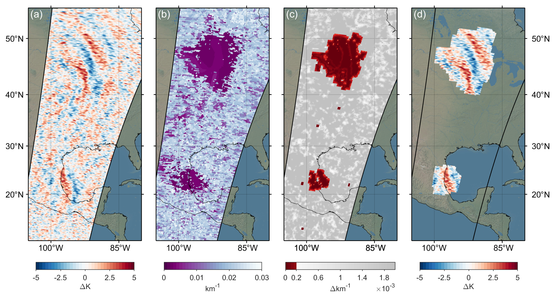
Figure 1 Step-by-step masking of two waves over North America, July 17th, 2010, granules 80–83. From left to right: (a) The temperature perturbations at 39 km altitude after preprocessing. (b) The horizontal wavenumbers found from the ST; the regions where the waves can be visually seen in the temperature perturbations appear as regions of similar wavenumber. (c) The average absolute difference between horizontal wavenumbers within each pixel's neighbourhood, the red indicates everywhere lower than the cutoff ($\mathrm{2}\times {\mathrm{10}}^{-\mathrm{4}}$ km⁻¹). (d) The final mask applied to the original temperature perturbations.

Areas of consistent wave properties at 39 km altitude are identified using the following methodology:

1. Pairs of granules are concatenated in the along-track direction (Fig. 1a.).

2. The ST technique is applied to the concatenated granules providing wavenumbers along-track, cross-track and in the vertical as functions of space. After that, the satellite track referenced wavenumbers are projected into zonal, meridional, and vertical wavenumbers k, l, and m. From this, it can be seen that GWs appear as regions of similar horizontal wavenumber amongst the noise, as illustrated by Fig. 1b.

3. For each pixel, the mean absolute difference between each pixel's horizontal wavenumbers (k and l) and the pixels in its 5×5 pixel adjacency neighbourhood is calculated. (Fig. 1c.). The reasoning for the size of the neighbourhood is discussed in Appendix A1.

4. In this proof of concept study, we apply a maximum tolerance of $C=\mathrm{2}\times {\mathrm{10}}^{-\mathrm{4}}$ km⁻¹ to this mean absolute difference field, as discussed in Appendix A2. Regions where wavenumbers are very similar in a 5×5 neighbourhood is consistent with our requirement for an extended GW field.

5. Contiguous positive-detection regions with an area smaller than three times the area of the neighbourhood (i.e. 75 voxels) are then removed from our dataset. This ensures that only plausible waves are detected, and removes small areas of coherent wavenumber noise (see Appendix A2 for more information).

6. Finally, the positive-detection regions are smoothed with a 5×5 window, from which a binary mask is created. This mask can be applied to any of the spectral outputs of the S-transformed smoothed data, such as in Fig. 1d.

3.3.2 Amplitude Cutoff Method

The amplitude cutoff method (Ern et al., 2017) is applied separately onto the spectral output of the S-transformed smoothed data. This method assumes that any temperature perturbations with amplitudes above the noise-floor of the data are associated with GWs. This study used an amplitude cutoff of 1.6 K, as this is the average retrieval noise at this altitude (39 km) (Hoffmann and Alexander, 2009; Hindley et al., 2019). A binary mask was generated, where areas with amplitudes greater than 1.6 K are classed as GWs, and areas lower than 1.6 K as noise. This is then applied onto any of the spectral outputs of the S-transformed data, as with the neighbourhood method.

3.4 Pseudo-momentum Flux

The pseudo-momentum flux (momentum flux, or MF) is then calculated for each pixel where a wave is detected using Eq. (1). MF is a derived value that characterises how much momentum is being transported by a GW (Fritts and Alexander, 2003; Ern, 2004), and thus how much potential drag (Ern et al., 2016) the waves have. Accurate estimates of MF are needed so that models can more precisely parameterise GWs. As derived by Ern (2004), this can be calculated as:

$$\begin{array}{}\text{(1)}& ({\mathrm{MF}}_x,{\mathrm{MF}}_y)=-{\displaystyle \frac{\mathit{\rho }}{\mathrm{2}}}{\left({\displaystyle \frac{g}{N}}\right)}^{\mathrm{2}}{\left({\displaystyle \frac{A}{\mathrm{BG}}}\right)}^{\mathrm{2}}\left({\displaystyle \frac{k}{m}},{\displaystyle \frac{l}{m}}\right)\end{array}$$

where ρ, g and N are density, acceleration due to gravity (9.69 ms⁻²), and the Brunt–Väisälä frequency (0.02 s⁻¹), respectively, A and BG are the temperature amplitude of the GW and the background temperature. We use the fourth-order polynomial that was fitted as the background temperatures. k,l and m are the horizontal and vertical wavenumbers that describe the wave. These are taken from the output of the ST. We can use this simplified version of the momentum flux equation as all of the GWs' intrinsic frequencies observed from AIRS lie within the mid-frequency approximation $\left(N\mathit{>>}\widehat{\mathit{\omega }}\mathit{>>}f\right)$, where f is the Coriolis parameter (Ern et al., 2017).

4 Results and discussion

We compare the results from the neighbourhood method to those from the amplitude cutoff method as detection methods for GWs in AIRS from 2010–2014.

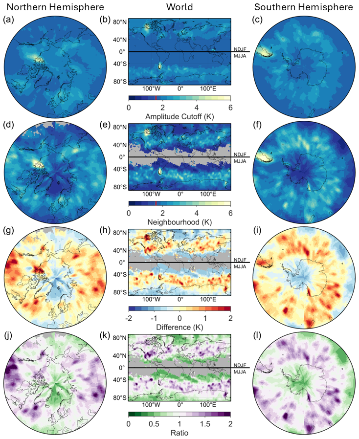
Figure 2 Maps showing mean detected GW amplitudes between 2010–2014 for the local winter months in both hemispheres (November, December, January, February and June, July, August, September). (a, b, c) GWs detected using the amplitude cutoff method, (d, e, f) GWs detected using the neighbourhood method, (g, h, i) the difference between amplitudes measured using the two methods, and (j, k, l) the amplitude ratio of the two methods.

Figure 2 shows a global comparison between the amplitude cutoff and neighbourhood methods. Specifically, it shows the mean amplitudes of detected GWs during local winter months, November–February (NDJF) for the Northern Hemisphere and May–August (MJJA) for the Southern Hemisphere. The differences (g, h, i) and ratios (j, k, l) between the two methods are also presented.

∼45 % of the areas where GWs were detected using the neighbourhood method shown here had an average amplitude below 1.6 K. This is possible because the ST can accurately categorise waves with low amplitudes, which the neighbourhood method then detects. Along the two lower stratospheric polar jets (Wright et al., 2017; Sato et al., 2012), the mean amplitude of GWs detected using the neighbourhood method is 1.13× greater than for GWs detected using the amplitude cutoff method, which corresponds to a mean difference of 0.28 K. This is because the amplitude cutoff method incorporates all the pixels with amplitudes above the defined cutoff, which can include noise. This brings the amplitudes' mean towards the noise amplitude's mean. We expect to detect more GWs in the lower stratospheric polar jets, as the GWs refract in the jets, increasing the GWs' vertical wavelengths. This elongation in the vertical allows them to be better resolved by AIRS (Wright et al., 2015).

Over some areas associated with strong GW activity (high amplitude waves with a clearly defined wave structure), such as over the Antarctic peninsula, we see only minor changes in amplitude between the two methods (Fig. 2g–i). This is due to the two methods detecting the same waves and converging on similar time-mean amplitudes.

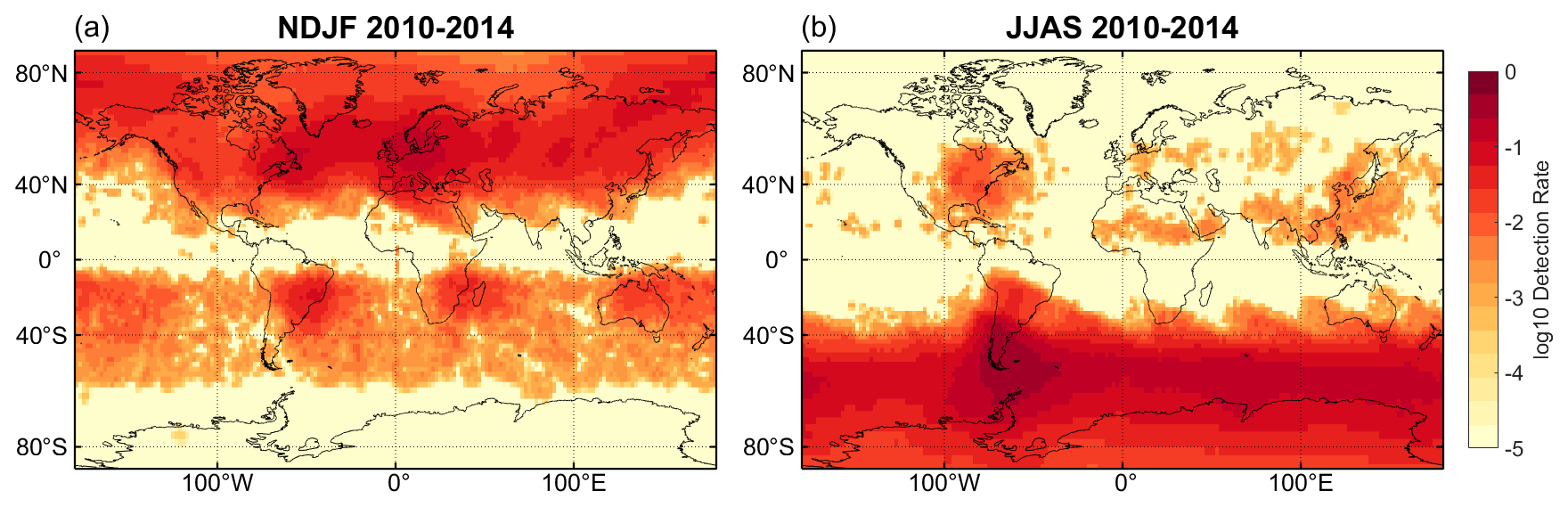
Figure 3 A map of the average wave detection rate at 39 km per AIRS overpass using the neighbourhood method. (a) shows boreal winter, November–February, and (b) austral winter, June–September. On a log10 scale.

Figure 3 shows the occurrence rate of GWs detected using the neighbourhood method, which we define as the average number of GWs detected over a 2° × 2° area per AIRS overpass. Compared to Figs. 6 and 7 of Hoffmann et al. (2013) (hereafter referred to as H13), who used a temperature variance method to detect GWs, Fig. 3 shows many of the same features and similar occurrence rates worldwide. There are some differences: GWs detected over the Southern Ocean in JJAS have a much higher occurrence rate in this figure than in H13, and there are waves detected nearly everywhere in the Northern Hemisphere in NDJF, whereas in H13 they were more sparse. The hotspots shown in H13's Figs. 14 and 15 exhibit a higher occurrence rate than that seen in our Fig. 3, but each hotspot is spatially smaller and these hotspots were spread across the world more than is seen in Fig. 3. These differences might be due to the H13 detection technique characterising peak events as having GW variance exceeding the zonal mean variance.

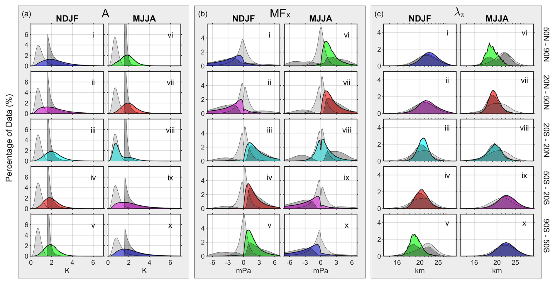
Figure 4 Histograms of GW variables from five different latitude bands during boreal winter (NDJF, i–v) and austral winter (MJJA, vi–x) between 2010–2014, presenting amplitude (a), zonal momentum flux (b), and vertical wavelength (c) from 39 km altitude. Each panel includes three histograms: light grey for the output of the ST with no additional detection method, dark grey for waves detected using the amplitude cutoff method, and coloured for waves extracted using the neighbourhood approach. Colours represent the season local to that latitude band. Each histogram has been internally normalised to sum to 100 % for ease of comparison. It is noted that the axis for vertical wavelength (c) is linear in wavenumber.

4.1 Histograms of Latitude Bands

Figure 4 shows histograms of GW amplitudes, zonal momentum flux, and vertical wavelengths for the three methods (i.e. ST output with no detection method, amplitude-cutoff and neighbourhood) of detecting GWs, in each panel for their respective season and latitude bands.

Each variable presented in Fig. 4 exhibits meridional changes (e.g. b.i–v) in the GWs detected using the neighbourhood method. This is equivalent to seasonal changes throughout the year. We hypothesise that this is due to the changing winds beneath the observation altitude (39 km) and the sources of GWs changing meridionally. These changes are seen as a movement of the curve's peak, or as a change in the curve's width. We individually discuss the three variables: amplitude, zonal momentum flux, and vertical wavelength.

4.1.1 Amplitude (A)

Figure 4a shows the normalised occurrence frequency of amplitudes from GWs detected using the amplitude cutoff and neighbourhood methods, as well as the amplitudes calculated from the ST with no additional detection method applied. During local winter, the histograms' for waves detected using the neighbourhood method consistently have a large proportion of data that are at lower amplitudes than for waves detected using the amplitude cutoff method, and slightly at greater amplitudes than those detected using only the ST. During local summer, the histograms' peaks for waves detected using the neighbourhood method are at greater amplitudes than those detected using the amplitude cutoff method. The mean percentage of regions of wave activity with amplitudes less than 1.6 K detected during local winter using the neighbourhood method is ∼35 % over all seasons and latitudes.

Strong meridional differences are apparent when using the neighbourhood method to extract amplitudes. There are a greater number of regions with higher-amplitude GWs during local wintertime than during local summertime, with $\sim \mathrm{31}\times$ more areas with waves having amplitudes greater than 2 K. This is a similar trend to the GWs detected using the amplitude cutoff, thus showing that both methods can accurately detect GWs with higher amplitudes.

4.1.2 Zonal Momentum Flux (MF_x)

When a GW's horizontal phase speed approaches the horizontal wind speed, the wave will undergo critical level filtering (Lindzen, 1981; Whiteway and Duck, 1996; Booker and Bretherton, 1967). This causes the wave to dissipate and deposit its energy and momentum into the background wind, changing the speed and direction of the background flow. The morphology of the coloured histograms presented in Fig. 4b is due to this phenomenon. For example, in Fig. 4b.i, the waves detected using the neighbourhood method have mainly negative MF_x, indicating that they propagate westwards. This concurs with ERA5 wind reanalysis data in this region at the altitude of this study (39 km), with the vast majority of wind being eastward. These results agree with the findings of Hindley et al. (2020).

The shape of the curves for MF_x calculated from waves detected using the neighbourhood method follows the same general morphology as those detected using the amplitude cutoff method, except that a greater proportion of waves detected using the neighbourhood method have a low absolute MF_x. This is because MF is proportional to amplitude squared (Eq. 1). Thus, the amplitude cutoff method cannot detect most waves with low absolute MF, whereas the neighbourhood method can detect most of these waves. The low percentage of data close to 0 mPa can be attributed to the fact that the neighbourhood method cannot identify waves with very small amplitudes due to the noise floor of AIRS. Another explanation might be that the waves mainly propagate in the zonal direction and hence, k is never close to 0.

Some waves detected using the neighbourhood method have MF_x in the direction of the general background wind, though this fraction is much smaller than with the other methods. These can be attributed to a variety of causes: the waves may have propagated meridionally and evaded a critical level, there may not have been a critical level for that particular wave where the waves propagated vertically, or the 3DST may have miscalculated the angle of propagation. The 3DST issue arises when the phase fronts of the GW are aligned near to the vertical; the technique must assign an angle relative to the vertical, and if that angle is nearly vertical, then errors can occur (Hindley et al., 2019).

In the tropics (Fig. 4b.iii, viii), the effects of the semiannual oscillation on the GWs (Smith et al., 2017) can be seen when using the neighbourhood method and the amplitude cutoff method. This pattern of eastward GWs during boreal winter and near symmetrical eastward/westward GWs during austral winter is consistent with Hindley et al. (2020). The background winds for this was also seen by Delisi and Dunkerton (1988).

4.1.3 Vertical Wavelength (λ_z)

The vertical wavelengths in Fig. 4c show a seasonal cycle when using the neighbourhood method. The peaks shift towards shorter vertical wavelengths and the distributions narrow as the local seasons change from winter to summer. For example, during boreal winter (Fig. 4c.i–v), the dominant wavelength changes from 22.2 km in the north to 18.7 km in the south, a difference of 3.5 km. The full-width half maximum during this period narrows, reducing by 62 % from 53 km in the north to 33 km in the south. The strong zonal background winds during local wintertime allow the long vertical wavelength waves observed here to propagate into the stratosphere (Hoffmann et al., 2013).

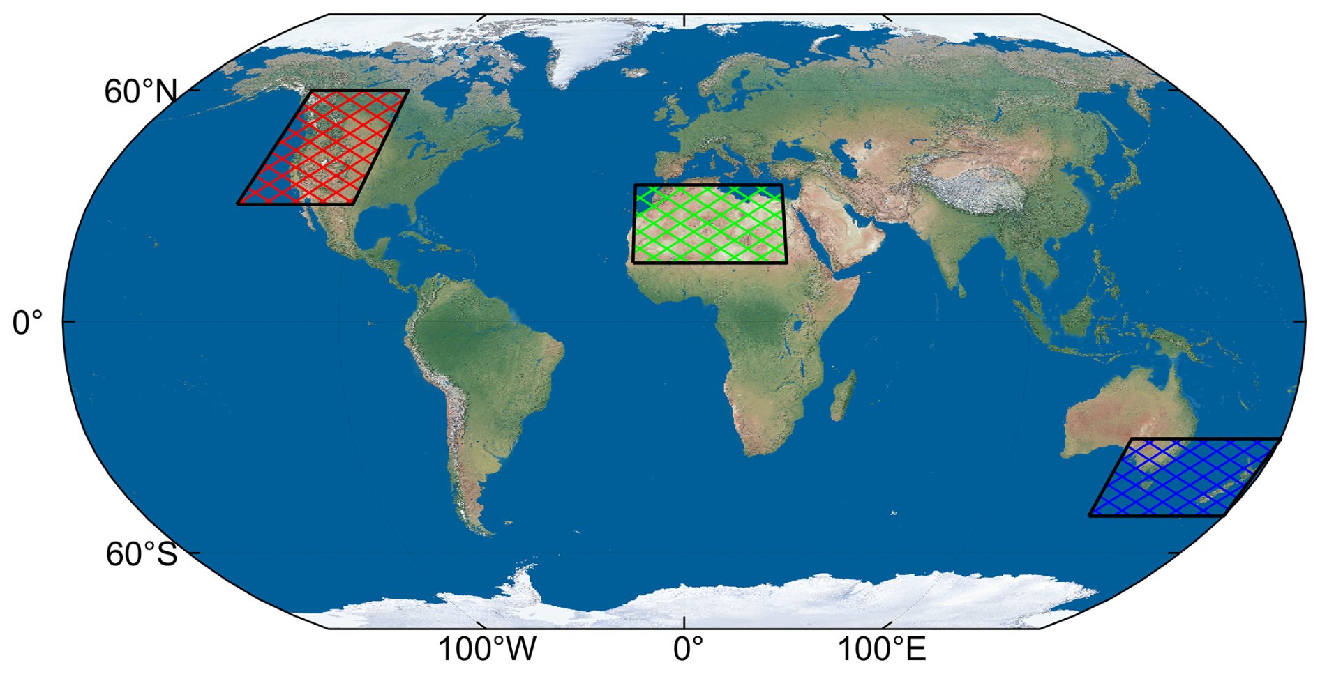
Figure 5 The regions chosen as case studies for this study. The Rocky Mountains, North Africa, and New Zealand/Tasmania.

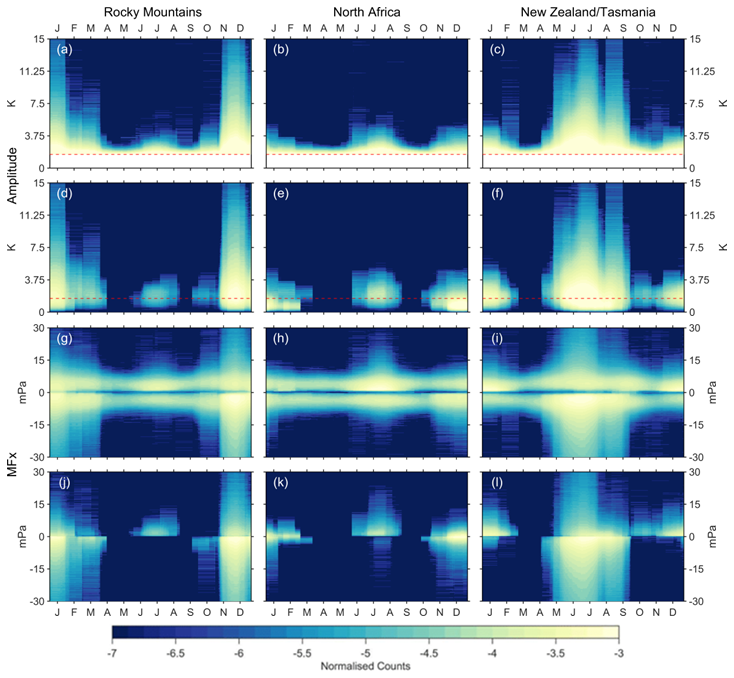
Figure 6 Histograms of normalised counts per day of the year (2010–2014), with a monthly-moving mean applied for each day, over the three regions: the Rocky Mountains (a, d, g, j), North Africa (b, e, h, k), and New Zealand/Tasmania (c, f, i, l) of amplitude (a–f) and zonal momentum flux (g–l). Panels (a)–(c) and (g)–(i) present the values of waves detected using the amplitude cutoff method, and panels (d)–(f) and (j)–(l) present the values of waves detected using the neighbourhood method. All waves are detected at 39 km. Colours are on a log10 scale, and have been normalised to sum to one. The red lines on panels (a)–(f) indicate the amplitude cutoff used.

4.2 Regional Studies

Three regions were chosen for deeper study (Fig. 5), specifically:

• The Rocky Mountains, which are a well-studied source of high GW activity (Lilly and Kennedy, 1973; Wang and Geller, 2003; Gong and Geller, 2010; Zhang et al., 2015; Wright and Banyard, 2020) with complex orography when compared to other regions (e.g. southern Andes) (Rapp et al., 2021; Reichert et al., 2021).

• North Africa, where studies have identified the main drivers of GW as the West African monsoon (Birch et al., 2012) and the Hoggar mountains (Orza et al., 2020), but in general, fewer studies have been carried out specific to the region when compared to the other two regions, and

• New Zealand and Tasmania, which was previously studied during the DEEPWAVE campaign (Bossert et al., 2017; Gisinger et al., 2017). Hoffmann et al. (2016) detected GWs over this region 13.5 % of the time in AIRS, with Eckermann and Wu (2012) and Pautet et al. (2019) finding that Tasmania is an important driver of GWs.

Figure 6 shows the annual cycle of GW activity over each region, where each column shows a distinct region. The top two rows (panels a–f) show the amplitudes of detected GWs for each region, with the first row (panels a–c) showing values calculated for GWs detected using the amplitude cutoff method, and the second row (panels d–f) showing values calculated from GWs detected using the neighbourhood method. The bottom two rows (panels g–l) show zonal momentum flux from GWs detected using the amplitude cutoff method (panels g–i) and the neighbourhood method (panels j–l). Each panel has been normalised to sum to 1.

Considering first the amplitudes of GWs detected using the amplitude cutoff method (panels a–c), the Rocky Mountains and New Zealand/Tasmania (panels a and c) exhibit similar morphologies, but offset by 6 months, with more higher amplitude GWs being detected during local winter, and becoming less frequent going into local summertime. There is a small peak in amplitudes during local summertime. This is consistent with the stratospheric wind reversal close to 20 km in summer, limiting the vertical propagation of orographic GWs. This may indicate that these regions have similar drivers of GWs, in this case orography (Wang and Geller, 2003; Gong and Geller, 2010; Bossert et al., 2017; Gisinger et al., 2017). Panel (b), which shows the same data but for GWs over North Africa, exhibits a semiannual cycle, peaking in local summer and winter. This cycle has a much lower mean amplitude than in the other two regions.

The amplitudes of GWs detected using the neighbourhood method (panels d–f) appear to follow the same pattern as in panels (a)–(c), but the continual low amplitude signal is not present. This allows the seasonal low-amplitude GWs to become more evident. The mean fraction of GWs detected using the neighbourhood method in these three regions with amplitudes below the amplitude cutoff is ∼45 %. These waves could not be detected using the amplitude cutoff method. There is a significant difference in the fraction of waves detected using the neighbourhood method between the Rocky Mountains and New Zealand during the local summer months, with a $\sim \mathrm{20}\times$ greater proportion of GW-containing regions detected over New Zealand (panel f). This may be due to the more stable winds around the South Pole than in the North during the summer, allowing GWs with a larger spectrum of phase speeds to propagate through, or because of the Southern Ocean storm belt interacting with the orography in New Zealand (Chapman et al., 2015; Shaw et al., 2022). In panel (e), GW activity from the West African monsoon is observed between June and August. Wright et al. (2011) demonstrated that monsoon-generated GWs in this region could be observed from HIRDLS satellite measurements.

The MF_x of GWs detected using the amplitude cutoff method shows roughly symmetrical results around 0 mPa for each region, with enhancements during the local winters and summers in the directions expected from theory. There is a lack of values close to 0 mPa for each region at all times of the year, consistent with Fig. 4. There is also a continual low MF_x signal in all regions and at all times of the year.

The MF_x calculated from GWs detected using the neighbourhood method (panels j–l) shows seasonal changes in GW activity. During local winter over the Rocky Mountains and New Zealand/Tasmania, the MF_x is mainly negative, corresponding with the westward propagating GWs against the background wind. The MF_x for North Africa in wintertime has a near-Gaussian distribution, which is not observed in the other regions analysed. The absolute values of MF_x for wintertime GWs detected using the neighbourhood method over North Africa are generally lower than those in the other two regions, between −4–3 mPa. Whereas the absolute values of MF_x detected using the amplitude cutoff method mainly have values between −7 to −0.7 and 1.3–7 mPa. The continuous low MF_x signal mentioned above is not present here, highlighting GW activity's seasonality.

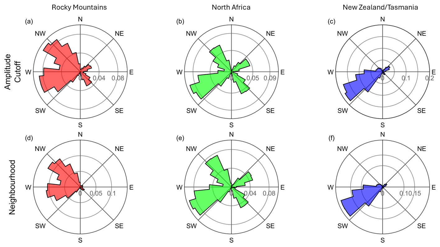
Figure 7 Polar histograms of wave phase propagation angles over the Rocky Mountains, North Africa, and New Zealand/Tasmania in local winter (NDJF for the Rocky Mountains and North Africa, and MJJA for New Zealand/Tasmania). Panels (a)–(c) show wave phase propagation angles for waves detected using the amplitude cutoff method, and panels (d)–(f) show wave phase propagation angles for waves detected using the neighbourhood method. Each histogram is normalised to sum to one.

We next consider Fig. 7, which shows polar histograms of wave phase propagation angle over the three regions for waves detected using the amplitude cutoff (panels a–c) and for waves detected using the neighbourhood method (panels d–f) during local wintertime. Panels (a) and (d) show results from the Rocky Mountains, panels (b) and (e) from North Africa, and panels (c) and (f) from New Zealand/Tasmania.

We primarily expect the waves observed in AIRS to propagate against the background wind (Alexander et al., 2009; Hindley et al., 2020). The wind is generally eastward for each region during this time due to the presence of the lower stratospheric polar night jet over the Rocky Mountains and New Zealand/Tasmania. Waves observed over these regions should primarily be propagating westwards.

The wave phase propagation angles for GWs detected using the neighbourhood method over the Rocky Mountains (panel d) are all approximately west-, and northwest-, wards, with the spread in values being potentially due to the Rocky Mountains not being a straight ridge (such as the Andes). The spread could also be due to the movement of the lower stratospheric polar night jet throughout the local wintertime. This is also seen for angles for GWs detected using the amplitude cutoff method (panel a), but with a greater spread, including more southwestward phase propagation angles. Significantly more waves propagate eastwards using the amplitude cutoff method than those detected using the neighbourhood method.

The tight spacing between the most south-westward waves for panel (f) (New Zealand/Tasmania) indicates that these waves propagate into the wind. This agrees with the findings of Smith et al. (2016), Jiang et al. (2019) and Pautet et al. (2019), whose results found that most GWs from New Zealand and Tasmania travel upwind, with wavefronts nearly perpendicular to the Southern Alps. Using ERA5 climatological reanalysis data, we found that the winds in this region during this period are directed north-eastwards, which agrees with these results. These findings can be seen when using the amplitude cutoff method (panel c), but with a tighter spread of results than those found using the neighbourhood method.

Waves over North Africa (panel e) show a similar spread in west-southwest phase propagation angles, although many waves propagate eastwards too. The prevailing winds over North Africa during this time flow eastwards at the altitude of this study, which was found using ERA5 climatological reanalyses and correlates with the primarily westwards phase propagation angles.

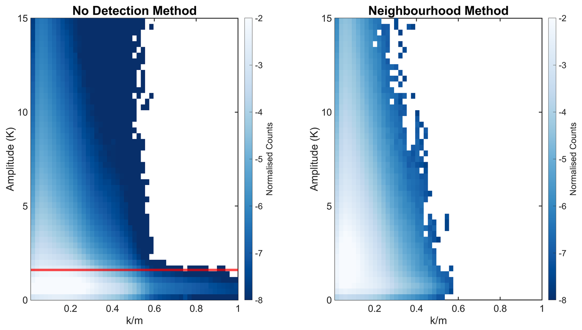
Figure 8 Density plots of the normalised counts for every day between 2010–2014, showing the relationship between amplitude and the ratio of zonal wavenumber to vertical wavenumber ($k/m$). Colours are on a log 10 scale. Panels (a) and (c) show these results from the ST output with no GW detection method applied, and panels (b) and (d) show the results from the ST output with the neighbourhood method applied. The red line on panel (a) is at the amplitude cutoff.

4.3 Sensitivity Analysis

Figure 8a and b show density maps of wave amplitude versus the zonal-to-vertical wavenumber ratio ($k/m$) for all data points so that we can compare sensitivities for the results for each method. Panel (a) includes all data without applying a GW detection method; the red line indicates the detection limit of the amplitude cutoff method – points below this line would be excluded. Panel (b) shows only the GWs detected using the neighbourhood method. Both methods capture a similar fraction of high-amplitude, low-$k/m$ waves. However, the neighbourhood method also detects many low-amplitude, low-$k/m$ waves that the amplitude cutoff method misses. Notably, the neighbourhood method does not detect any waves with $k/m$ values greater than 0.6, which is reasonable, as larger values would mean the GWs have unreasonably sized wavelengths. This shows that the neighbourhood method is sensitive to GWs with low and high amplitudes and to GWs with $k/m$ values from 0 to 0.6. The amplitude cutoff method can not observe the low amplitude waves, but it captures the same spread of $k/m$ values as using the neighbourhood method.

5 Conclusions

In this study, a method for detecting stratospheric GWs in AIRS/Aqua observations was developed, which we refer to as the “neighbourhood method”. This uses a variant of the 3D S-transform to calculate the horizontal wavenumbers of temperature perturbations, then find areas of spatially near-constant horizontal wavenumbers (assumed to be GWs), which allow for the creation of a binary wave-presence mask. This allows us to produce a new global climatology of GW properties and, in particular, identify key results that are accessible using this method, which could not be achieved using older techniques. To quantify this, we have applied the neighbourhood method and the existing widely-used amplitude cutoff method to 5 years of data between 2010–2014.

Analysing these data, we conclude that:

• About 35 % of all regions with GWs detected using the new neighbourhood method could not be detected using the older amplitude cutoff method, and would be indistinguishable from instrument noise if neither method were applied. In regions dominated by low-amplitude GW activity, such as North Africa, this difference increases to as much as ∼81 % of all areas with GWs. In contrast, in other regions dominated by strong orographic waves, such as New Zealand and the Rockies, the fraction is lower, ∼32 % and ∼21 % respectively.

• The meridional change of GWs' vertical wavelengths can be seen when using the neighbourhood method. It presents as a change in the dominant wavelength of 3.5 km from the summer hemisphere to the winter hemisphere and as a widening of the full-width half maximum by 62 %.

• Net zonal momentum fluxes and angles for GWs detected using the neighbourhood method exhibit plausible directionality compared to theory, especially when corroborated against ERA5 background winds.

• The neighbourhood method is sensitive to waves with all amplitudes within a reasonable range of $k/m$ values (0–0.6). The amplitude cutoff method is only sensitive to waves with amplitudes larger than its cutoff (1.6 K), with the same range of $k/m$ values as the neighbourhood method.

The neighbourhood method can be used on any data that can be S-transformed from nadir-sounding instruments, with minor changes to the parameters needed for each instrument to get the most accurate GW detections. In particular, the outputs from the neighbourhood method could be used to make GW parameterisations in models more accurate, especially over regions of typically low-amplitude waves. In addition, they could support backwards ray-tracing of GWs, or be used as a training set for a large-scale convolutional neural network. We are investigating the latter option, and have presented this in a companion paper (Okui et al., 2025).

Appendix A: Values used in the Neighbourhood Method

There are two variables that must be chosen as fixed values in the neighbourhood method: the neighbourhood size, and the wavenumber difference cutoff. These must be set to maximise the amount of real GW information, but minimise the amount of noise present. The perfect values for these variables vary greatly on a case-by-case basis, so for broad application we must empirically-determine values that suit the majority of waves. A decision was made to be conservative with the size and number of waves detected, to be confident that all of the detected signals contained only waves, and we note clearly that different tuning parameters could detect more waves, but at a greater cost in terms of false positives.

A1 Neighbourhood Size

Figure A1 shows the case study described in Fig. 1, with four different neighbourhood sizes used for the wave detection. Using a small, 3×3, neighbourhood (panel a), the neighbourhood method detects too many waves, most of which cannot be seen in the temperature perturbations. Panels (c) (7×7) and (d) (9×9) appear to have stabilised around the large wave in the North, but they do not capture the GW over Central America. Only panel (b) (5×5) detects both waves visible in the temperature perturbations and no extra noise. This analysis was done for multiple other cases, and the 5×5 neighbourhood was chosen.

A2 Average Difference Cutoff

Using the 5×5 neighbourhood chosen in Appendix A1, the average difference cutoffs were varied. For clarity, the larger the cutoff, the more, and larger, waves would be expected to be detected. This is seen in Fig. A2; panel (a) uses a cutoff of $\mathrm{0.5}\times {\mathrm{10}}^{-\mathrm{4}}$ km⁻¹ and detects the smallest total area of waves, but it does not detect any noise. This was deemed to be too conservative. Panel (d) uses a cutoff of $\mathrm{0.1}\times {\mathrm{10}}^{-\mathrm{2}}$ km⁻¹, which has the same issue as in Fig. A1a of detecting too many waves. Using many other cases, $\mathrm{2}\times {\mathrm{10}}^{-\mathrm{4}}$ km⁻¹ was chosen as the average difference cutoff used on the dataset.

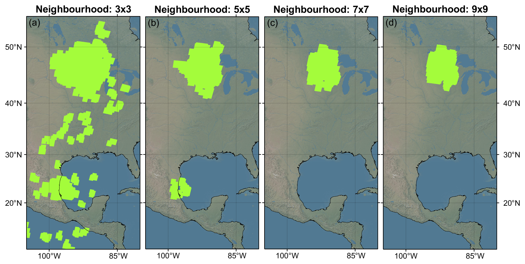
Figure A1 Various neighbourhood sizes for the case study described in the method.

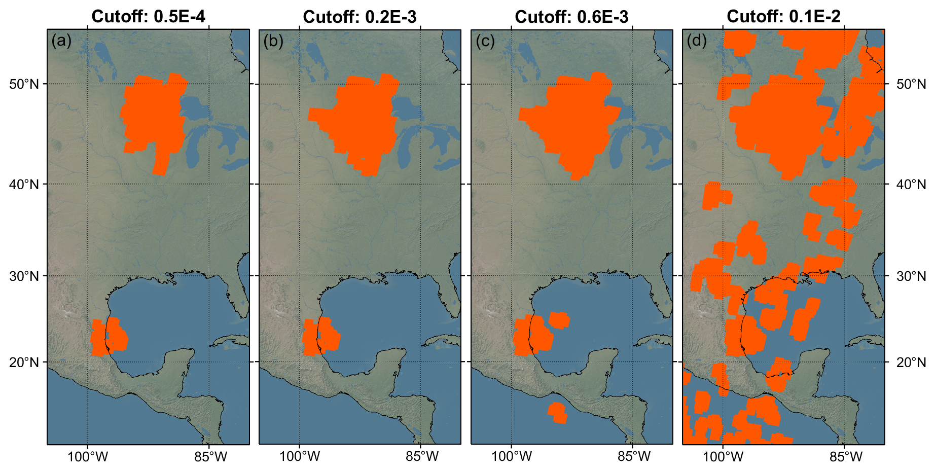
Figure A2 Various average difference cutoffs for the case study described in the method.