Evidence for the role of thermal and cloud merging in mesoscale convective organization

Observations from airborne field campaigns are used to study the interplay between boundary-layer thermals and clouds in the trades. The size distributions of thermal and cloud-base chords inferred from turbulence and horizontal lidar-radar measurements are robustly described by the sum of two exponentials. Analytical calculations and statistical simulations show that the merging of objects is sufficient to explain the two exponentials, representing, respectively, the populations of merged- and unmerged-object chords. They also show how circulations induced by convective objects facilitate the merging process. The observed day-to-day variability of these populations at cloud base can thus be tied to the variability of thermal merging across the depth of the subcloud layer. Clouds rooted in unmerged thermals are small and shallow while those rooted in merged thermals are wider and deeper. An intricate interplay between thermal- and cloud-merging arises: when thermal merging is weak, thermal number density is high and cloud bases merge easily, leading to strong mesoscale mass fluxes and “Gravel” shallow mesoscale organizations. In contrast, when thermal merging is strong, clouds are fed by sparser but wider thermals, leading to longer cloud lifetimes but weaker cloud merging, weaker mesoscale mass fluxes, and “Flower” mesoscale organizations. This interplay between thermal- and cloud-merging imposes an upper bound on cloud coverage and suggests a negative feedback on the growth of mesoscale circulations. Thermal merging also controls observed size distributions of thermals in deep convective regimes. The merging process thus appears to be a fundamental player in the mesoscale organization of convection.

1 Introduction

Moist convection generates a broad spectrum of cumulus clouds of varying widths, depths, and spacings. In regimes of shallow convection, this spectrum is dominated by two cloud types: very shallow clouds, whose tops do not exceed a few hundred meters above the cloud base, and deeper clouds, whose tops can reach several kilometres and often precipitate (Byers and Hall, 1955; Nuijens et al., 2014; Albright et al., 2023; Vial et al., 2023). By interacting with each other and with their environment, these clouds organize on the mesoscale (2–200 km, Agee, 1987). Deeper clouds, for instance, tend to be wider and more widely spaced than shallow clouds (Joseph and Cahalan, 1990) owing to their compensating subsidence, which inhibits the growth of nearby clouds (Bretherton, 1987). The development of deeper clouds is tied to the growth of shallow mesoscale circulations, which further reinforces their organization (Bretherton and Blossey, 2017; Narenpitak et al., 2021; Janssens et al., 2023). Taken together, this suggests a coordination between the emergence of different cloud types, cloud organizations, and mesoscale circulations.

Taking a bottom up view, convective cloud formation is rooted in coherent structures such as thermals that develop within the subcloud layer (LeMone and Pennell, 1976; Cohen and Craig, 2006; Seifert and Heus, 2013). The emergence of cloud types and organizations must therefore be related to changes in these structures. The natural place to study this interaction is at the intersection of the subcloud layer and cloud layer, i.e. at cloud base. The properties at cloud base are known to strongly control the fate of clouds. For instance, cloud widths at cloud base influence the turbulent entrainment at the edge of clouds (Blyth, 1993) and hence the cloud penetration depth (Malkus and Ronne, 1954; Simpson et al., 1965; Asai and Kasahara, 1967), and they are the primary modulator of the strength of convective mass fluxes (Böing et al., 2012; Dawe and Austin, 2012). These cloud widths are likely related to the sizes of thermals that permeate the subcloud layer, suggesting a coupling between thermal sizes, cloud types, cloud organizations, and mesoscale circulations.

Indeed, modeling studies have shown the interplay between thermal sizes, cloud base widths, and convective mass fluxes to play a major role in the transition between shallow and deep convection (Kuang and Bretherton, 2006; Khairoutdinov and Randall, 2006; Böing et al., 2012; Rochetin et al., 2014; Rousseau-Rizzi et al., 2017; Morrison et al., 2022), and it has long been recognized that cloud size distributions at the cloud base level are a fundamental variable to understand and represent cumulus convection (Simpson et al., 1965; Asai and Kasahara, 1967; Ooyama, 1971; Arakawa and Schubert, 1974; Craig and Cohen, 2006; Sakradzija et al., 2015; Neggers and Griewank, 2022). However, thermal and cloud base size distributions have largely been studied in large-eddy simulations and in ground-based observations over land (e.g. Neggers et al., 2003; Chandra et al., 2013; Lamer and Kollias, 2015; Lareau et al., 2018; Öktem and Romps, 2021). Observations over the ocean are much more limited (López, 1977; LeMone and Zipser, 1980).

The wealth of observations collected during the EUREC⁴A (Elucidating the role of cloud-circulation coupling in climate) airborne field campaign over the western tropical Atlantic (Bony et al., 2017; Stevens et al., 2021) present an opportunity to conduct such an investigation in the context of trade wind cumuli. The campaign provided observations of both clouds and their environment, including of the mesoscale circulations in which they were embedded (George et al., 2023). More specifically, it characterized shallow convection for a month using a statistical sampling strategy in a region characterized by a large diversity and variability of mesoscale cloud patterns, the most prominent of which are commonly referred to as “Sugar”, “Gravel”, “Fish”, or “Flowers” (Stevens et al., 2020; Bony et al., 2020; Rasp et al., 2020; Janssens et al., 2021; Schulz, 2022). While the “Sugar” pattern consists exclusively of very shallow clouds, the other patterns are associated with a combination of shallow and deeper clouds in varying proportions and degrees of clustering (Mieslinger et al., 2019; Bony et al., 2020; Vial et al., 2021, 2023; Alinaghi et al., 2024).

In this study, we primarily use EUREC⁴A observations (presented in Sect. 2) to shed light on the interplay between thermals, clouds, mass fluxes and mesoscale circulations. First we characterize the size distributions of thermal chords (Sect. 3) and cloud-base chords (Sect. 4), and show that they can be described as a mixture of two chord populations and fitted by a sum of two exponentials. Section 5 uses an analytical framework, mathematical calculations and a simple statistical model to show that the double exponential size distributions can be physically interpreted as the result of the merging process. In Sect. 6, we show how the length scales of cloud size distributions relate to those of thermals. Finally, we take advantage of the analytical framework, the statistical sampling of EUREC⁴A and the large flight-to-flight variability of cloudiness, to further characterize the interplay between thermals and clouds, and explore its implications for convective mass fluxes and shallow mesoscale circulations, cloud mesoscale patterns and cloud fraction (Sect. 7). In Sect. 8, we summarize our main findings, investigate their universality by using the first observations from a field campaign that took place in regimes of both shallow and deep convection, and discuss the perspectives of this study.

2 Airborne observations

The EUREC⁴A field campaign (Bony et al., 2017; Stevens et al., 2021) took place in January–February 2020 in the North Atlantic trades, east of Barbados. In this study, we use observations from the SAFIRE ATR-42 (Bony et al., 2022) and from the HALO (Konow et al., 2021) research aircraft.

Over 4 weeks, the ATR conducted 18 research flights across 10 flight days, and spent most of its flight time near cloud base and within the subcloud layer. Each flight was 4.5 or 5 h long and followed a common flight pattern including typically two or three rectangles of about 120 km × 20 km flown around the cloud-base level (totaling 48 rectangles, i.e. about 36 h of sampling) plus two L-shape patterns of about 120 km each flown within the subcloud layer. Most of the time, an additional leg of about 40 km long was flown about 60 m above the sea surface.

The aircraft measured turbulence (including horizontal and vertical velocity, inferred from the measurements of a five-hole nose radome) and humidity at a fast rate (25 Hz) using a Licor near-infrared gas analyzer and a KH20 hygrometer (Brilouet et al., 2021). At a flight speed of about 100 m s⁻¹, this corresponds to an horizontal resolution of about 4 m. The humidity data used in the present analysis come from 30 km (5 min) stabilized flight segments (referred to as “short segments”). They correspond to calibrated, detrended and high-pass filtered (at 0.018 Hz) perturbations of water vapor mixing ratio (Brilouet et al., 2021). The payload also included a 355 nm backscatter lidar pointing horizontally through one of the aircraft windows (ALIAS, Chazette et al., 2020) and a Doppler cloud radar (BASTA, Delanoë et al., 2016) pointing horizontally through another window on the same side of the aircraft (Bony et al., 2022). This remote sensing allowed us to sample clouds horizontally over a much larger domain than in-situ measurements. The lidar could detect hydrometeors over a maximum range of 8 km, while the radar could detect non-drizzling clouds over a range of 3 to 6 km and drizzling clouds and rain up to 12 km. By combining horizontal radar-lidar measurements, we characterized the horizontal distribution of hydrometeors at a resolution of 25 m along the line of sight of both instruments (BASTALIAS dataset, Delanoë et al., 2021; Bony et al., 2022).

During ATR flights, HALO was flying large circles of 200 km diameter at an altitude of 10 km, releasing dropsondes every 5 min (Konow et al., 2021). From these measurements, we inferred the subcloud layer height (Albright et al., 2022), the area-averaged cloud-base mass flux (Vogel et al., 2022) and, using the methodology proposed by Bony and Stevens (2019), the vertical profiles of area-averaged vertical velocity (George et al., 2021) and the strength of shallow mesoscale circulations (George et al., 2023). From the multiple downward-looking instruments mounted on HALO (cloud radar, lidar and imagers), a multi-sensor cloud mask product was derived (Konow et al., 2021). We use the maximum cloud cover estimated on the basis of the “most likely” and “probably” cloud flags of each instrument.

At the end of this study, we also use the first airborne observations from the MAESTRO (Mesoscale organisation of tropical convection, https://maestro.aeris-data.fr/, last access: 14 June 2025) field study that took place in August–September 2024 over the Eastern tropical Atlantic in the vicinity of Cape Verde. During this campaign, the SAFIRE ATR-42 aircraft sampled a wide diversity of convective regimes, ranging from shallow to deep convection. Its fast-rate humidity measurements (Jaffeux et al., 2025) allow us to characterize, as in EUREC⁴A, the thermal chord length distributions at different vertical levels and to assess the universality of some of our findings across regions and convective regimes.

3 Convective thermals

In the trade-wind boundary-layer, water vapor is mixed vertically by turbulent eddies and discrete coherent structures, including moist, ascending anomalies which are called thermals. When the air parcels transported by the thermals reach the condensation level, they condense and form a cloud. We might thus expect the size characteristics of cloud bases to be related to the size of thermals permeating the subcloud layer.

Table 1 Thermals observed during EUREC⁴A in the surface layer, the subcloud layer and near cloud base: For each ATR flight, f^TH is the thermal coverage, 𝒟^TH is the thermal density (in km⁻¹), N^TH is the number of chords, and $p_{\mathrm{1}}^{\mathrm{TH}}$ ($p_{\mathrm{2}}^{\mathrm{TH}}=\mathrm{1}-p_{\mathrm{1}}^{\mathrm{TH}}$), $L_{\mathrm{1}}^{\mathrm{TH}}$ and $L_{\mathrm{2}}^{\mathrm{TH}}$ (in meters) are the parameters of the double exponential fit (see Eq. 1). In the surface layer, the fit is close to a single exponential. Therefore, for the sake of space we report only 𝒟^TH, N^TH and $L_{\mathrm{1}}^{\mathrm{TH}}$. The flights (or flight segments) without data are indicated by “–”: no turbulence data are available for RF20 (failure of the inertial navigational system) and on the near-surface leg of RF14 (humidity measurements of bad quality), the near-surface was not sampled by the aircraft in RF05, RF07, RF08, RF09 and RF17, and the subcloud layer was not sampled during RF16.

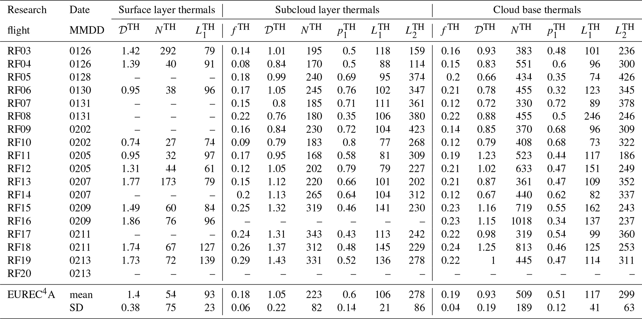
To identify moist thermals from airborne measurements, we use the methodology proposed by Lenschow and Stephens (1980): segments of horizontal legs with humidity greater than half the standard deviation of humidity fluctuations for that leg, and larger than 25 m (i.e. 6 continuous data points), are defined as thermals. This detection is applied to all humidity fluctuations measured along 30 km segments (Brilouet et al., 2021) flown at different altitudes: near the sea surface (at a height of about 60 m, 11 flights), within the sub-cloud layer (in the middle of it – around 300 m – and near the top of it – around 600 m, 16 flights) and just above the cloud base level (between 600 and 800 m, 17 flights). Hereafter, for simplicity, the length of each thermal segment, or chord, will sometimes be referred to as “thermal size”.

Statistics over the whole EUREC⁴A campaign show that the mean thermal density (i.e. the number of intersected segments of thermals per horizontal distance flown by the aircraft) is largest near the surface (about 1.4 thermals km⁻¹) and smaller aloft, with about 1 thermal km⁻¹ in the middle of the subcloud-layer and near cloud base (Table 1). On the other hand, the mean size of thermals increases with height, varying from 93 m near the surface to about 200 m at the top of the subcloud layer. This can reflect the growth of individual thermals by entrainment or the coalescence of small thermals into larger ones as they rise and merge in the sub-cloud layer (Sect. 5.2). Around the cloud base level, cloudy thermals (identified as those thermals in which every point in it has a relative humidity exceeding 98 %) represent about 18 % of the thermal population at that level, and their size is on average slightly smaller than the mean size of moist thermals (∼160 m vs. 200 m), which is consistent with Lenschow and Stephens (1980).

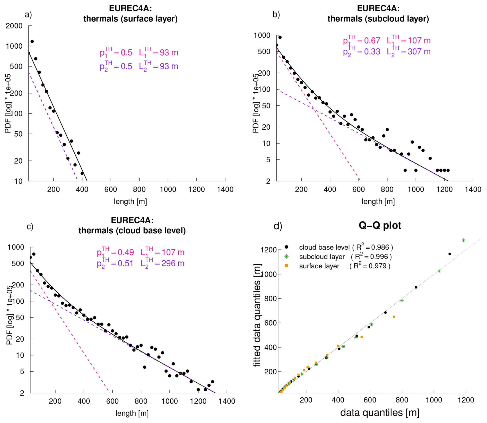
Figure 1 Thermal size distributions: Probability Distribution Function (PDF) of thermal chord lengths inferred from all EUREC⁴A ATR turbulence measurements at different altitudes: (a) 60 m above the surface (b) within the sub-cloud layer (around 300 or 600 m) and (c) near cloud base (around 750 m). Also reported is the exponential fit (simple or mixture) and its parameters ($p_{\mathrm{1}}^{\mathrm{TH}}$, $p_{\mathrm{2}}^{\mathrm{TH}}$, $L_{\mathrm{1}}^{\mathrm{TH}}$ and $L_{\mathrm{2}}^{\mathrm{TH}}$, Eq. (1) – note that this fit is very similar to the one obtained using the mean fit parameters (averaged over all flights) reported in Table 1). (d) Comparison of the quantiles of the actual and fitted size distributions (Q-Q plot). Also reported are the R² coefficients (square of the Pearson correlation coefficients) of the linear regression for each flight level.

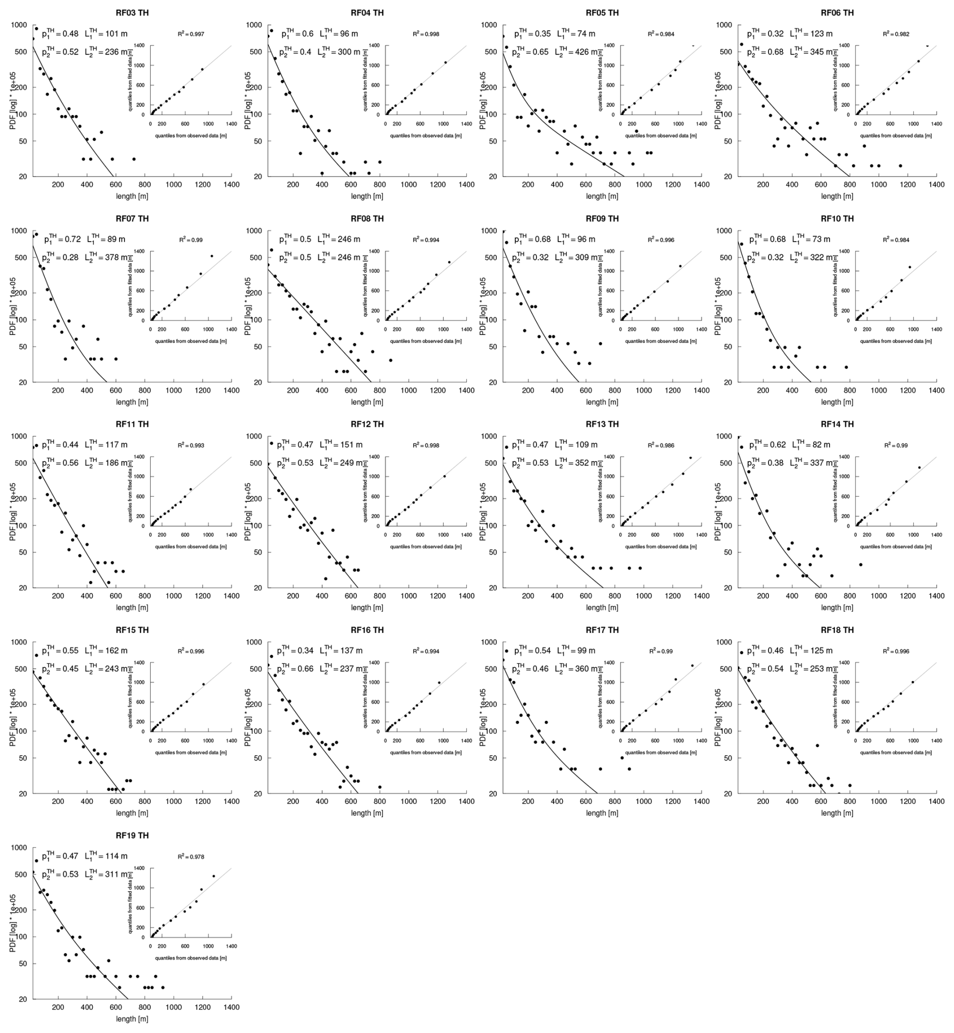
Figure 2 Thermals from each EUREC⁴A flight: Probability distribution functions of the thermal chord lengths (in meters) derived for each ATR flight from turbulence measurements around the cloud base level (the distribution derived from all ATR flights together is shown on Fig. 1c). Each panel shows the histogram, its fit by a sum of two exponentials (solid line) and the associated Q-Q plot (inset) to assess how well the sum of exponentials fits the data. The parameters of the fit ($p_{\mathrm{1}}^{\mathrm{TH}}$, $L_{\mathrm{1}}^{\mathrm{TH}}$, $p_{\mathrm{2}}^{\mathrm{TH}}$, $L_{\mathrm{2}}^{\mathrm{TH}}$) are also reported.

However, at each altitude, the thermal dimensions exhibit a wide range of lengths. Near the surface, the length ranges from 25 m (the minimum size considered in our definition of thermals) to about 400 m, and the likelihood of finding a thermal of a given size decays exponentially with size (Fig. 1). At higher altitudes, the probability distribution function (PDF) of chord lengths P(x) is well fitted¹ by a mixture of two exponential functions with relative weights p₁ and $p_{\mathrm{2}}=\mathrm{1}-p_{\mathrm{1}}$, and characterized by length scales L₁ and L₂ (Rochetin et al., 2014), such as :

$$\begin{array}{}\text{(1)}& P\left(x\right)={\displaystyle \frac{p_{\mathrm{1}}}{L_{\mathrm{1}}}}{e}^{-\frac{x}{L_{\mathrm{1}}}}+{\displaystyle \frac{p_{\mathrm{2}}}{L_{\mathrm{2}}}}{e}^{-\frac{x}{L_{\mathrm{2}}}}.\end{array}$$

This suggests that the thermal chord ensemble is well described by a mixture of two thermal populations, of mean sizes $L_{\mathrm{1}}^{\mathrm{TH}}$ (about 100 m) and $L_{\mathrm{2}}^{\mathrm{TH}}$ (about 300 m). The comparison of the quantiles associated with the actual and fitted size distributions (so-called Q-Q plots shown on Fig. 1d and Fig. 2) confirms that this description is not only valid when considering all EUREC⁴A data but also robust at the scale of individual flights, though the relative weight and mean size of each population vary across flights (Table 1). Following these notations, the mean size of thermal chords is given by $L=p_{\mathrm{1}}{L}_{\mathrm{1}}+p_{\mathrm{2}}{L}_{\mathrm{2}}$. Moreover, if N is the total number of thermal chords intersected by the aircraft along a horizontal distance of ℒ, the mean thermal density (𝒟) for this distance is given by $N/\mathcal{L}$.

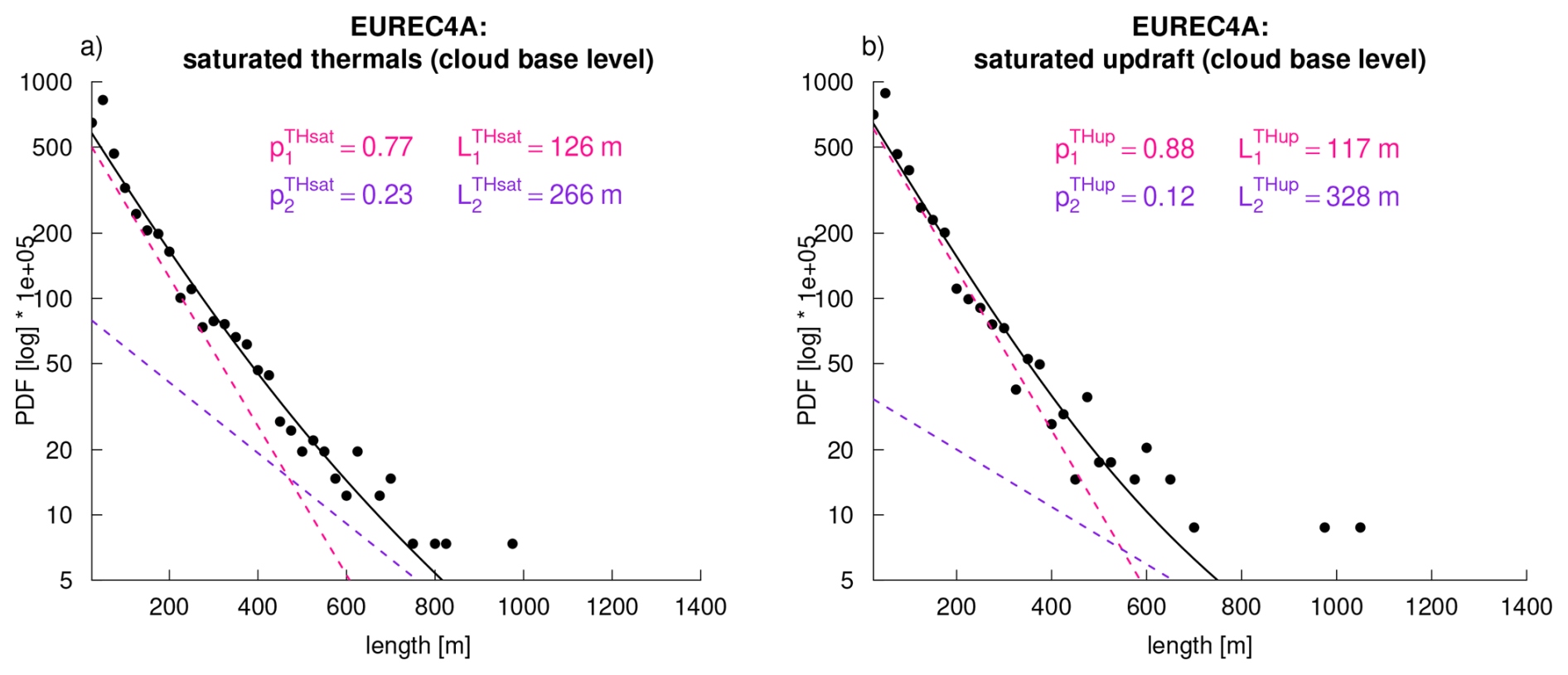
Figure 3 Probability distribution function of (left) cloudy thermal lengths and (right) cloudy updraft lengths measured by the ATR near the cloud-base level. Cloudy thermals are defined as moist thermals (or segments) whose points are saturated near the cloud base level (relative humidity exceeding 0.98), and cloudy updrafts are defined as cloudy thermals whose points all have a positive vertical velocity near cloud base.

Thermals that overshoot the lifting condensation level (LCL) generate saturated thermal chords, or “cloudy thermals”. The majority of these (84 % in the EUREC⁴A data) are characterized by a mean positive vertical velocity (“cloudy updrafts”). They may therefore be regarded as “cloud shoots”, i.e. incipient cloud bases formed immediately after thermals overshoot the LCL, that can subsequently grow into convective clouds rooted in boundary layer thermals. Figure 3 shows that their size distribution is also well fitted by a mixture of two populations, and that their length scales $L_{\mathrm{1}}^{\mathrm{THsat}}$ and $L_{\mathrm{2}}^{\mathrm{THsat}}$ for cloudy thermals, and $L_{\mathrm{1}}^{\mathrm{THup}}$ and $L_{\mathrm{2}}^{\mathrm{THup}}$ for cloudy updrafts, are comparable to those of the whole thermal population (Fig. 1c). Flight-to-flight variations in the density of cloudy thermals (𝒟^THsat) and cloudy updrafts (𝒟^THup) are strongly correlated with each other (R²=0.96), and also with the total density of thermals 𝒟^TH (R²=0.74 and 0.70, respectively, Fig. S5 in the Supplement). On average, however, 𝒟^THsat and 𝒟^THup are five to six times smaller than 𝒟^TH, with a mean ratio ${\mathcal{D}}^{\mathrm{THsat}}/{\mathcal{D}}^{\mathrm{TH}}=\mathrm{0.18}$ and ${\mathcal{D}}^{\mathrm{THup}}/{\mathcal{D}}^{\mathrm{TH}}=\mathrm{0.15}$ in the EUREC⁴A dataset. Therefore, to increase the statistical robustness of our investigations, in the following sections of this study we will analyze the flight-to-flight variations in thermal populations and size distributions by considering all moist thermals.

4 Cloud-base widths

EUREC⁴A pioneered the sampling of clouds through horizontal remote sensing thanks to sidewards-looking radar and lidar measurements across the ATR windows (Bony et al., 2022). Using the hydrometeors classification derived from the synergy of the lidar-radar remote sensing over a range of several kilometers away from the aircraft (Delanoë et al., 2021; Bony et al., 2022), we detect the length of cloud segments, or chords, along the line of sight of the lidar-radar measurements, perpendicular to the aircraft trajectory. The horizontal resolution of the hydrometeors classification along the line of sight of the radar and lidar is 25 m. A segment (or chord) corresponds to at least 2 continuous points associated with cloud or drizzle, i. e. reflectivities lower than 0 dBZ (drizzle is considered because the distinction between clouds and drizzle using radar reflectivity is ambiguous, and because drizzle falls within cloud base in the case of shallow cumuli). Horizontal remote sensing makes it possible to characterize the size distribution of cloud chords (hereafter referred to as “cloud-base widths”) through the sampling of one or multiple chords within each cloud, without having to determine whether chords sampled at different times belong to the same cloud or not. This allows us to characterize the irregular and complex shapes of cloud bases without making assumptions about cloud shapes, and to sample the cloud field around the cloud base level with much better horizontal sampling than would be possible with in-situ measurements along the aircraft's trajectory.

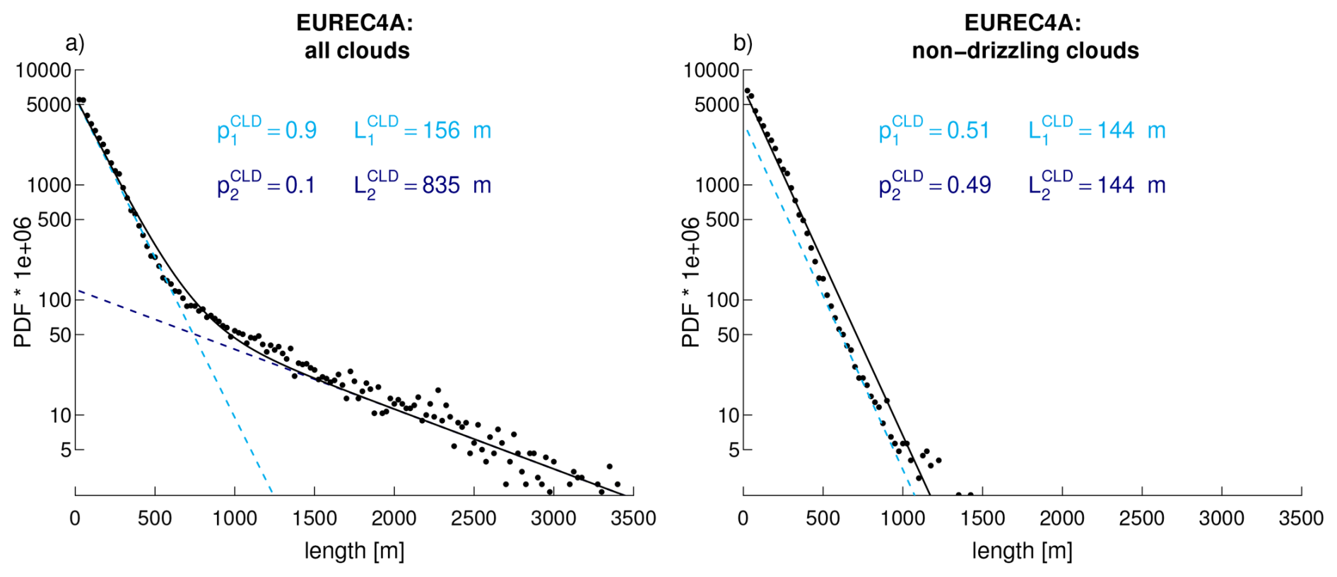
Figure 4 Cloud chord length distributions derived from horizontal radar-lidar measurements around cloud base: (a) PDF obtained by considering all EUREC⁴A flights together fitted by a mixture of two exponential distributions (Eq. 1). (b) Same as (a) but for cloud chords devoid of drizzle. The parameters reported on each panel are those associated with each fit.

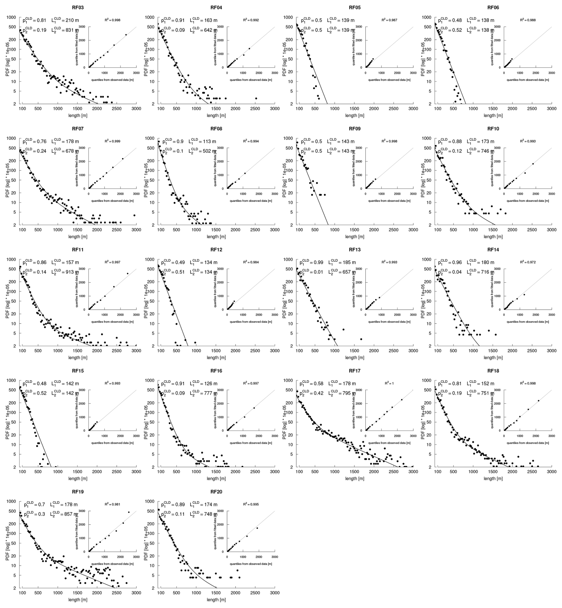
Figure 5 Clouds from each EUREC⁴A flight: Probability distribution functions of the cloud chord lengths (in meters) derived for each ATR flight from horizontal radar-lidar measurements around the cloud base level. Each panel shows the histogram, its fit by a sum of two exponentials (solid line) and the associated Q-Q plot and R² (inset) to assess the goodness of fit. The parameters of the fit ($p_{\mathrm{1}}^{\mathrm{CLD}}$, $L_{\mathrm{1}}^{\mathrm{CLD}}$, $p_{\mathrm{2}}^{\mathrm{CLD}}$, $L_{\mathrm{2}}^{\mathrm{CLD}}$) are also reported.

The cloud chord length distribution computed over the whole EUREC⁴A campaign shows the presence of many small chords and fewer larger chords (Fig. 4a). As for thermals, the distribution is well fitted by a mixture of two populations with $p_{\mathrm{1}}^{\mathrm{CLD}}=\mathrm{0.9}$ and $p_{\mathrm{2}}^{\mathrm{CLD}}=\mathrm{1}-p_{\mathrm{1}}^{\mathrm{CLD}}=\mathrm{0.1}$. Each population is characterized by an exponential length distribution, with a scaling parameter corresponding to the average length of the chords in that population: $L_{\mathrm{1}}^{\mathrm{CLD}}=\mathrm{156}$ m, and $L_{\mathrm{2}}^{\mathrm{CLD}}=\mathrm{835}$ m.

However, the comparison of the different flights reveals that as for thermals, the cloud chord distribution varies strongly from flight to flight. Figure 5 shows that for each individual flight, the distribution is still robustly fitted by a mixture of exponential distributions, but in variable proportions and with scaling parameters $L_{\mathrm{1}}^{\mathrm{CLD}}$ and $L_{\mathrm{2}}^{\mathrm{CLD}}$ that can vary significanly across flights (Table 2).

Table 2 Cloud chords measured during EUREC⁴A near cloud base: For each ATR flight, f^CLD is the cloud fraction, N^CLD is the number of chords, and $p_{\mathrm{1}}^{\mathrm{CLD}}$ ($p_{\mathrm{2}}^{\mathrm{CLD}}$ = 1 - $p_{\mathrm{1}}^{\mathrm{CLD}}$), $L_{\mathrm{1}}^{\mathrm{CLD}}$ and $L_{\mathrm{2}}^{\mathrm{CLD}}$ (in meters) are the parameters of the bi-exponential fit (see Eq. 1). Note that $L_{\mathrm{1}}^{\mathrm{CLD}}\approx L_{\mathrm{2}}^{\mathrm{CLD}}$ corresponds to a single exponential. Also reported is the rain fraction during each flight (R_f, in %).

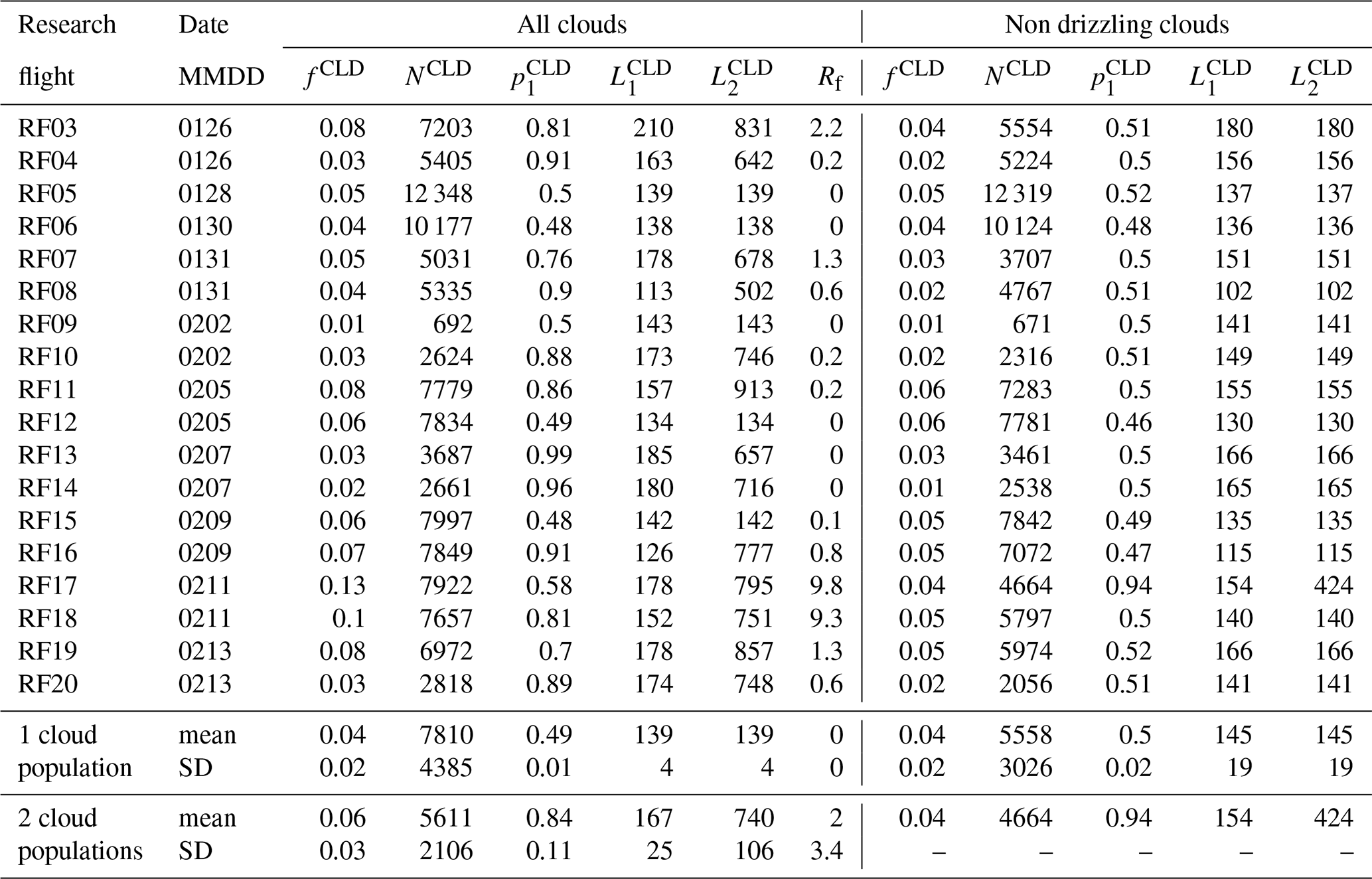
The variability of the cloud chord distributions around cloud base correlates with a number of cloud properties. Firstly, the clouds encountered on flights with only one cloud population (5 out of 18) are devoid of drizzle, and for each flight, the PDF of cloud chords devoid of drizzle is well fitted by a single exponential (Figs. 4b, S3). Since drizzle starts when the cloud depth exceeds about 2 km (Byers and Hall, 1955; Rauber et al., 2007), it suggests that the first cloud mode is associated with very low cloud tops, while the second mode includes cloud chords which are not only larger but also associated with deeper cloud tops than those of the first population.

These observations suggest that the two shallow cloud populations (very shallow and deeper) reported in previous studies (i.e. Albright et al., 2023; Vial et al., 2023) are characterized by two populations of cloud chords at the cloud base level. The length scale of the first cloud mode $L_{\mathrm{1}}^{\mathrm{CLD}}$ (about 150 m) is only slightly smaller than the mean chord length of thermals (170 m in the subcloud layer, 204 m at cloud base), and comparable to the mean chord length of saturated thermals (about 160 m) or cloudy updrafts (about 150 m). It suggests that this cloud population might be rooted in single boundary-layer thermals reaching the condensation level. On the other hand, when there are two distinct cloud populations (i.e. when $L_{\mathrm{2}}^{\mathrm{CLD}}\ne L_{\mathrm{1}}^{\mathrm{CLD}}$) the length scale of the second one $L_{\mathrm{2}}^{\mathrm{CLD}}$ is 739 m on average, which is close to the mean subcloud-layer depth of 725 m (Bony et al., 2022). $L_{\mathrm{2}}^{\mathrm{CLD}}$ is thus 4 or 5 times larger (depending on flights) than the mean thermal length of cloudy thermals (L^THsat) or updrafts (L^THup), which suggests that the second cloud population is fed by several thermals. In the following, we investigate what controls the length scales of these different populations, and how the thermal and cloud chord length distributions relate to each other.

5 Influence of the merging process

EUREC⁴A observations show that the thermal density decreases with increasing altitude (Table 1), and that the size distribution of thermals changes across the depth of the boundary layer: a single population of thermal chords, whose size is exponentially distributed, is found in the surface layer while two chord populations are found higher up in the subcloud layer and near cloud base (Fig. 1). How to interpret these observed features?

Based on the theory of fluctuations in an equilibrium convective ensemble, Craig and Cohen (2006) showed that a population of convective objects in statistical equilibrium with its large-scale environment is characterized by an exponential size distribution as long as the objects do not strongly interact with each other. However, it has long been suggested that convective thermals progressively group and merge together with height as they rise through the depth of the subcloud layer (Lenschow and Stephens, 1980; Williams and Hacker, 1993). Simpson et al. (1980) also “postulated merging to be a major way in which convective clouds become larger”. Then the question arises as to whether the second population of thermals or clouds (whose average size is several times that of the first population, Tables 1 and 2) might arise from the interaction of thermals or clouds through a merging process.

If we consider that two objects merge if and only if they touch each other, simple physical reasoning suggests that the efficiency of merging depends on the ratio between the initial average object length L₀ and the average object spacing ${\mathit{\lambda }}_{\mathrm{0}}=\mathrm{1}/{\mathcal{D}}_{\mathrm{0}}$, where 𝒟₀ is the object density before merging (in the following, the attribute “0” will always refer to quantities before merging).

However, fluid mechanical laboratory experiments and simulations have long demonstrated that turbulent thermals and plumes can interact and merge at a distance due to friction and entrainment at their boundaries, ambient horizontal flow or wind shear, buoyancy-induced pressure gradients (Batchelor, 1954; Pera and Gebhart, 1975; Brahimi and Doan-Kim-Son, 1985; Kaye and Linden, 2004; Rooney, 2016; Mei and Yuan, 2021), and, as we consider further here, the updraft-induced circulation that they create around them (Bretherton, 1987; Poujol, 2025). As explained in Appendix A and in the Supplement, this is equivalent to considering that the merging takes place between effective objects of size βL₀ with β≥1, where β is referred to as an effective factor. For the time being, this parameter can be physically interpreted as the radius of influence an object exerts on other objects through the circulation it induces. Further physical interpretations will be presented in Sect. 6.2.

These physical arguments suggest that the product β𝒟₀L₀ describes a merging efficiency. Then, how does the thermal size distribution depend on β𝒟₀L₀? We first address this problem mathematically (Sect. 5.1), and then with a simple numerical statistical model (Sect. 5.2).

5.1 Analytical calculations

Let us consider a population of objects (that we will name “thermals” in the following, but they could be clouds or updrafts in general) randomly placed in space following a uniform distribution, characterized by an averaged length L₀, a density 𝒟₀, and an exponential size distribution:

$$\begin{array}{}\text{(2)}& {\mathbb{S}}_{\mathrm{0}}\left(x\right)={\displaystyle \frac{\mathrm{1}}{L_{\mathrm{0}}}}{e}^{-\frac{x}{L_{\mathrm{0}}}}\end{array}$$

For the reasons explained above and in Appendix A, it is assumed that the merging takes place between objects of effective size βL₀ with β≥ 1. It is possible to compute the size distribution of thermals after merging, by distinguishing the two types of thermals that emerge: those that have merged and those that have not merged yet. The analytical treatment (detailed in the Supplement) shows that after letting the thermals merge once or several times, the size distribution of the thermals that have not merged is written:

$$\begin{array}{}\text{(3)}& {\mathbb{S}}_{\mathrm{unmerged}}\left(x\right)={\displaystyle \frac{\mathrm{1}}{L_{\mathrm{1}}}}{e}^{-\frac{x}{L_{\mathrm{1}}}}\text{with}{L}_{\mathrm{1}}={\displaystyle \frac{L_{\mathrm{0}}}{\mathrm{1}+\mathit{\beta }{\mathcal{D}}_{\mathrm{0}}{L}_{\mathrm{0}}}}\end{array}$$

and the size distribution of the thermals that have merged is asymptotically exponential for large thermal sizes (x ≫ L₀):

$$\begin{array}{}\text{(4)}& {\mathbb{S}}_{\mathrm{merged}}\left(x\right)={\displaystyle \frac{\mathrm{1}}{L_{\mathrm{2}}}}{e}^{-\frac{x}{L_{\mathrm{2}}}}\text{with}{L}_{\mathrm{2}}=L_{\mathrm{0}}{e}^{\mathit{\beta }{\mathcal{D}}_{\mathrm{0}}{L}_{\mathrm{0}}}\end{array}$$

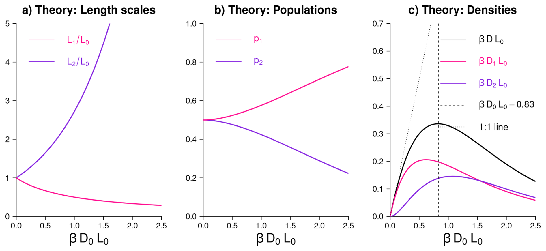
Figure 6 Theoretical prediction of the impact of merging on the size distribution and densities of chords: The efficiency of the merging process is quantified by β𝒟₀L₀, where 𝒟₀, L₀ and βL₀ are the initial density, length scale and effective length scale of chords before merging. L_i and p_i are the chord length distribution parameters (as defined by Eq. 1) of the chords that have merged (L₂, p₂) or not merged yet (L₁, p₁). Also reported are the unmerged, merged and total densities 𝒟₁, 𝒟₂ and $\mathcal{D}={\mathcal{D}}_{\mathrm{1}}+{\mathcal{D}}_{\mathrm{2}}$ of chords after merging. The proportion of chords in the first and second populations are given by ${\mathcal{D}}_{\mathrm{1}}/({\mathcal{D}}_{\mathrm{1}}+{\mathcal{D}}_{\mathrm{2}})$ and ${\mathcal{D}}_{\mathrm{2}}/({\mathcal{D}}_{\mathrm{1}}+{\mathcal{D}}_{\mathrm{2}})$, respectively. Note that length scales and densities are undimensioned through a multiplication by $\mathrm{1}/L_{\mathrm{0}}$ and βL₀, respectively.

Moreover, analytical expressions are also derived for the density of unmerged thermals, 𝒟₁, and the density of merged thermals, 𝒟₂, as follows:

$$\begin{array}{}\text{(5)}& {\displaystyle }{\mathcal{D}}_{\mathrm{1}}={\mathcal{D}}_{\mathrm{0}}{\displaystyle \frac{e^{-\mathit{\beta }{\mathcal{D}}_{\mathrm{0}}{L}_{\mathrm{0}}}}{\mathrm{1}+\mathit{\beta }{\mathcal{D}}_{\mathrm{0}}{L}_{\mathrm{0}}}}\text{(6)}& {\displaystyle }{\mathcal{D}}_{\mathrm{2}}={\displaystyle \frac{\mathrm{1}-e^{-\mathit{\beta }{\mathcal{D}}_{\mathrm{0}}{L}_{\mathrm{0}}}\left(\mathrm{1}+\frac{\mathit{\beta }{\mathcal{D}}_{\mathrm{0}}{L}_{\mathrm{0}}}{(\mathrm{1}+\mathit{\beta }{\mathcal{D}}_{\mathrm{0}}{L}_{\mathrm{0}}{)}^{\mathrm{2}}}\right)}{\mathit{\beta }{L}_{\mathrm{0}}(\mathrm{1}+e^{\mathit{\beta }{\mathcal{D}}_{\mathrm{0}}{L}_{\mathrm{0}}})}}\end{array}$$

After merging, the size distribution of thermals can thus be written as a sum of two exponential functions as written in Eq. (1), with L₁ and L₂ defined as above and $p_{\mathrm{1}}+p_{\mathrm{2}}=\mathrm{1}$. The calculations indicate that:

$$\begin{array}{}\text{(7)}& {\displaystyle }{p}_{\mathrm{1}}={\displaystyle \frac{\mathrm{1}}{\mathrm{1}+(\mathrm{1}+\mathit{\beta }{\mathcal{D}}_{\mathrm{0}}{L}_{\mathrm{0}})e^{-\mathit{\beta }{\mathcal{D}}_{\mathrm{0}}{L}_{\mathrm{0}}}}}\text{(8)}& {\displaystyle }{p}_{\mathrm{2}}={\displaystyle \frac{(\mathrm{1}+\mathit{\beta }{\mathcal{D}}_{\mathrm{0}}{L}_{\mathrm{0}})e^{-\mathit{\beta }{\mathcal{D}}_{\mathrm{0}}{L}_{\mathrm{0}}}}{\mathrm{1}+(\mathrm{1}+\mathit{\beta }{\mathcal{D}}_{\mathrm{0}}{L}_{\mathrm{0}})e^{-\mathit{\beta }{\mathcal{D}}_{\mathrm{0}}{L}_{\mathrm{0}}}}}\end{array}$$

These calculations, illustrated by Fig. 6, thus show that the merging of thermals that are characterized initially by an exponential size distribution of length scale L₀ produces a second population of thermals, and that the size distribution of the thermal population after merging can be represented by the sum of two exponential functions, characterized by two length scales L₁ and L₂. In the absence of merging (β𝒟₀L₀=0), $L_{\mathrm{1}}=L_{\mathrm{2}}=L_{\mathrm{0}}$ (Fig. 6a) and $p_{\mathrm{1}}=p_{\mathrm{2}}=\mathrm{0.5}$ (Fig. 6b): the size distribution can be represented by a single exponential. However, as the merging efficiency β𝒟₀L₀ increases, L₁ decreases (because the smaller thermals are statistically less likely to be affected by the merging process) while L₂ increases (because the merging produces larger thermals).

The total density of thermals after merging (𝒟, which is always ≤ 𝒟₀) is the sum of the densities of non-merged and merged thermals. Using Eqs. (5) and (6), we obtain the following analytical expression:

$$\begin{array}{}\text{(9)}& \begin{array}{rl}\mathcal{D}& ={\mathcal{D}}_{\mathrm{1}}+{\mathcal{D}}_{\mathrm{2}}\\ & \approx {\displaystyle \frac{{\mathcal{D}}_{\mathrm{0}}{e}^{-\mathit{\beta }{\mathcal{D}}_{\mathrm{0}}{L}_{\mathrm{0}}}}{\mathrm{1}+\mathit{\beta }{\mathcal{D}}_{\mathrm{0}}{L}_{\mathrm{0}}}}+{\displaystyle \frac{\mathrm{1}-e^{-\mathit{\beta }{\mathcal{D}}_{\mathrm{0}}{L}_{\mathrm{0}}}\left(\mathrm{1}+\frac{\mathit{\beta }{\mathcal{D}}_{\mathrm{0}}{L}_{\mathrm{0}}}{(\mathrm{1}+\mathit{\beta }{\mathcal{D}}_{\mathrm{0}}{L}_{\mathrm{0}}{)}^{\mathrm{2}}}\right)}{\mathit{\beta }{L}_{\mathrm{0}}(\mathrm{1}+e^{\mathit{\beta }{\mathcal{D}}_{\mathrm{0}}{L}_{\mathrm{0}}})}}\end{array}\end{array}$$

Solving the equation $\frac{\partial {\mathcal{D}}_{\mathrm{1}}}{\partial \left(\mathit{\beta }{\mathcal{D}}_{\mathrm{0}}{L}_{\mathrm{0}}\right)}=\mathrm{0}$ shows that there is an optimal $\left(\mathit{\beta }{\mathcal{D}}_{\mathrm{0}}{L}_{\mathrm{0}}\right)=\frac{\mathrm{1}}{\mathit{\phi }}\approx \mathrm{0.618}$ (where $\mathit{\phi }=\frac{\mathrm{1}+\sqrt{\mathrm{5}}}{\mathrm{2}}$ is the golden number) which maximizes the total number of non merged thermals, and that 𝒟 reaches a maximum value ${\mathcal{D}}_{\mathrm{crit}}\approx \frac{\mathrm{0.34}}{\mathit{\beta }{L}_{\mathrm{0}}}$ for $\mathit{\beta }{\mathcal{D}}_{\mathrm{0}}{L}_{\mathrm{0}}={\left(\mathit{\beta }{\mathcal{D}}_{\mathrm{0}}{L}_{\mathrm{0}}\right)}_{\mathrm{crit}}=\mathrm{0.83}$. There is therefore a critical merging efficiency of thermals beyond which the merging becomes so efficient in producing larger but fewer thermals that the densities of thermals before and after merging become anti-correlated (Fig. 6c). In other words, the 𝒟−β𝒟₀L₀ curve is concave down, with a local maximum at β𝒟₀L₀=0.83.

Although the physical meaning of L₁ and L₂ is clear (these length scales relate to the mean chord lengths of unmerged and merged thermals, respectively), the physical meaning of p₁ and p₂ is not so clear. When β𝒟₀L₀→0 (i. e., no merging), Eq. (8) and Fig. 6b show that L₁=L₂ and $p_{\mathrm{1}}=p_{\mathrm{2}}=\mathrm{0.5}$. However, when L₁=L₂, any values of p₁ and p₂ satisfying p₁ + p₂ = 1 (including p₁=1 and p₂=0) would describe the same (single) exponential size distribution. Therefore, p₂ should not be interpreted as the proportion of thermals in the second population (it is just an asymptotic approximation) and the ratio $\frac{{\mathcal{D}}_{\mathrm{2}}}{{\mathcal{D}}_{\mathrm{1}}+{\mathcal{D}}_{\mathrm{2}}}$ is a better measure of the proportion of merged thermals than p₂. In addition, the influence of merging on the size distribution is best described by L₂−L₁ or (as will be shown later, Fig. 8b) by the non-dimensional quantity $\frac{L_{\mathrm{2}}-L_{\mathrm{1}}}{\mathrm{2}{L}_{\mathrm{0}}}$, and the absence of merging is best described by L₂→L₁ or by the density of merged thermals 𝒟₂→0.

These calculations thus support our hypothesis that the second exponential of the size distribution results from the merging process. Reciprocally, they also show that it is possible to infer the properties of the thermal population before merging from the size distribution of thermals after merging (characterized by L₁ and L₂): by combining Eqs. (3) and (4) to eliminate L₀, we obtain:

$$\begin{array}{}\text{(10)}& \mathit{\beta }{\mathcal{D}}_{\mathrm{0}}{L}_{\mathrm{0}}=W_L\left(e{\displaystyle \frac{L_{\mathrm{2}}}{L_{\mathrm{1}}}}\right)-\mathrm{1}\end{array}$$

where W_L is the Lambert W function satisfying x=W(x)e^W(x) and

$$\begin{array}{}\text{(11)}& L_{\mathrm{0}}=L_{\mathrm{2}}{e}^{-\mathit{\beta }{\mathcal{D}}_{\mathrm{0}}{L}_{\mathrm{0}}}\text{or}{L}_{\mathrm{0}}\approx \sqrt{L_{\mathrm{1}}{L}_{\mathrm{2}}}\end{array}$$

(the second expression for L₀ is obtained after a multiplication of Eqs. 3 and 4, followed by a first order Taylor expansion of the exponential function). Moreover, as shown in the Supplement, the coverage fraction of thermals can be expressed as:

$$\begin{array}{}\text{(12)}& f={\displaystyle \frac{\mathrm{1}}{\mathit{\beta }}}(\mathrm{1}-e^{-\mathit{\beta }{D}_{\mathrm{0}}{L}_{\mathrm{0}}}).\end{array}$$

Therefore it is possible to infer β in the observations from Eqs. (10) and (12).

5.2 Simple statistical simulations

Although analytical calculations support the hypothesis that the merging process is sufficient to explain the presence of a mixture of exponential distributions, they are based on a number of mathematical simplifications that were needed to make the calculations tractable. Therefore we test the validity of the theory and further test the hypothesis that merging can explain the second population of chords in the size distribution of thermals, by developing a simple one dimensional statistical model.

We assume that initially the thermals are uniformly and randomly distributed along a domain of length L_domain=1000 km with a mean spacing ${\mathit{\lambda }}_{\mathrm{0}}=\mathrm{1}/{\mathcal{D}}_{\mathrm{0}}$, following a Poisson process, and that they have an exponential size distribution (Eq. 2) of characteristic size L₀=100 m (this value is chosen to be close to the averaged thermal length measured in the surface layer, Fig. 1a). For the sake of simplicity, we assume β=1.

The thermals are placed onto the domain one at a time. Everytime one is placed, it is checked whether the new thermal overlaps with an already existing thermal. If so, then these thermals are merged such that the edges of the new thermal is the leftmost extent of the leftmost old thermal and the rightmost extent of the rightmost old thermal (Fig. A1 in the Appendix), as assumed also in the mathematical calculations. After the merging processes takes place, the coverage fraction is counted. If this coverage fraction is less than a pre-specified value f_TH, then the simulation proceeds by placing a new thermal, checking for overlap, merging if there is overlap, then computing the coverage fraction again. This continues until the coverage fraction in the simulation equals f_TH. Once they are equal, the simulation is ended. The simulation is then repeated 10 times to generate more statistics. The thermal positions and lengths are recorded both before and after the merging process takes place.

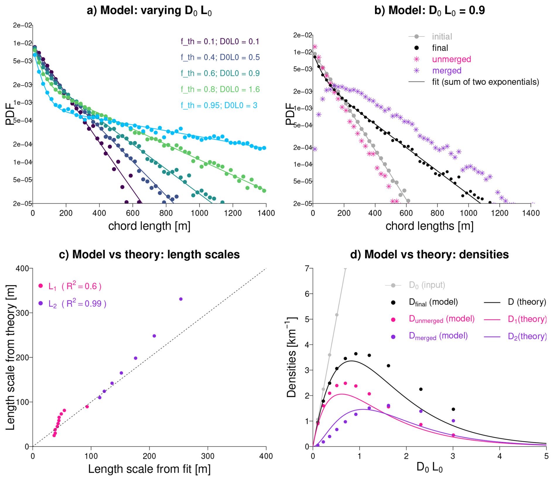
Figure 7 Simple statistical model of chord merging: (a) Chord length distributions obtained for L₀=100 m, β=1 and different values of f_TH (or, equivalently, for a range of β𝒟₀L₀ values), fitted by a sum of two exponential functions (solid lines). (b) For a particular value of the merging efficiency (β𝒟₀L₀ = 0.9 or f_TH=0.6), comparison of the chord length distributions of thermals before merging (in grey) and after merging, considering all thermals (in black) or just those that have merged (in purple) or that remain unmerged (in pink). The initial and unmerged thermals are well fitted by a single exponential distribution while the distribution of merged thermals tends asymptotically (for chord lengths ≫ L₀) towards an exponential distribution. (c) Comparison of the distribution length scales L₁ (in pink) and L₂ (in purple) predicted by theory or actually obtained from the fit of chord length distributions for a range of β𝒟₀L₀ values. (d) Comparison between the simple statistical model and the theory of the chord density 𝒟 after merging, and its decomposition into 𝒟₁ (unmerged, in pink) and 𝒟₂ (merged, in purple). The chord density before merging (𝒟₀, in grey) is also reported.

Figure 7a shows the chord length distributions obtained through this process for a range of f_TH values, which (from Eq. 12) amounts to a range of β𝒟₀L₀ values and thus of merging efficiencies. In the case of weak merging efficiency, the final distribution is close to the initial exponential distribution. However, for stronger merging efficiencies we note the formation of larger chords and an increasing deviation from the initial distribution, with the formation of a long tail. Each final distribution turns out to be well fitted by a sum of two exponentials. As merging is the only process represented in this model, it shows that if the initial size distribution of thermals is exponential, merging is a sufficient process to explain the formation of a second population of larger thermals and produce a final chord length distribution that is well fitted by a double exponential.

This is further confirmed by Fig. 7b that shows the decomposition of the size distribution into merged and unmerged thermals for a given merging efficiency. Although the size distribution of the thermals that have not merged yet is exponential and associated with a shorter lengthscale than the initial distribution (L₁<L₀), the size distribution of the thermals that have merged tends, for large chord lengths, to an exponential distribution. This is in line with the theory that predicts that the distribution of merged thermals is only asymptotically exponential (that is, for lengths much larger than L₀).

We then use the simple model to assess the ability of the analytical calculations to predict L₁, L₂ and the thermal densities. Although not perfect, we note a fairly good agreement between simulations and theoretical predictions, both for the length scales (Fig. 7c) and for the evolution of the densities of merged and unmerged thermals with the merging efficiency (Fig. 7d). These results give us confidence in the validity of the analytical treatment, and encourage us to use this theory to interpret the observations.

6 Interplay between thermals and clouds

6.1 Thermal merging inferred from observations

Given that trade wind clouds are rooted in subcloud layer thermals (LeMone and Pennell, 1976), we now investigate how the merging of boundary layer thermals imprints the size distribution of clouds near their base. For this purpose, we first assess the extent to which the physical framework presented in Sect. 5 can help interpret EUREC⁴A observations (summarized in Tables 1 and 2). From Eqs. (10) and (11) and the length scales L₁ and L₂ inferred from the observed chord length distributions, we infer L₀ and 𝒟₀. From Eq. (12) and the fractional coverage of thermals or clouds measured for each flight, we infer β. Then, from the values of (𝒟₀, L₀, β) associated with each flight, we compute the density of thermals expected from the theory (Eq. 9) and compare it with the density that was actually measured during the campaign.

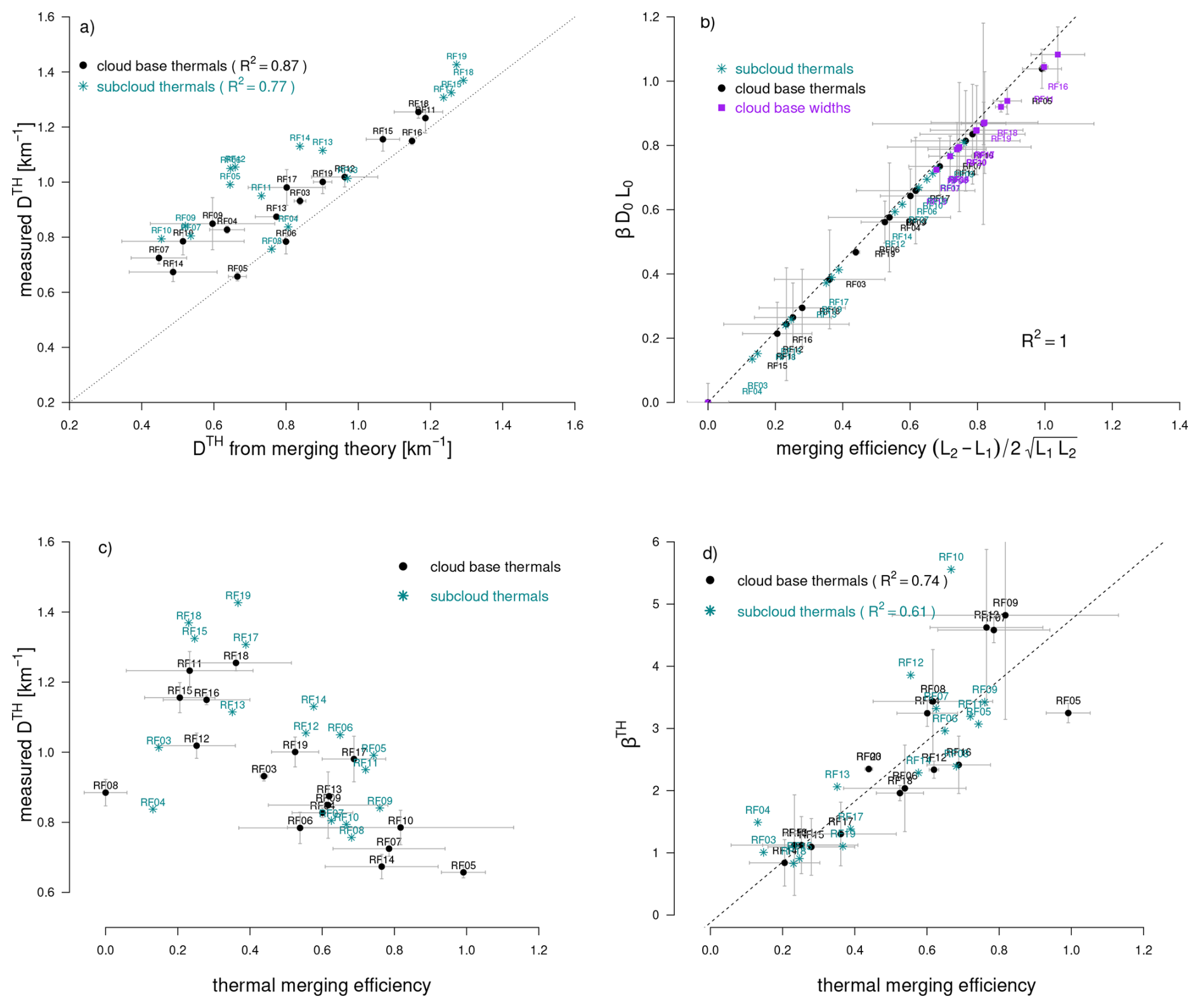
Figure 8 Consistency between theory and observations: (a) Comparison of the density of thermals after merging derived from turbulence measurements or predicted from theory using Eq. (9). Each point represents one ATR research flight (Table 1). Horizontal and vertical bars represent errors on the mean calculated from the measurements associated with the different rectangles flown near cloud base. Turquoise and black markers correspond to thermals sampled in the subcloud layer and near the cloud base, respectively. (b) Relationship (shown for thermals and clouds) showing the equivalence between the theoretically defined merging efficiency β𝒟₀L₀ and the quantity $(L_{\mathrm{2}}-L_{\mathrm{1}})/\left(\mathrm{2}{L}_{\mathrm{0}}\right)$ derived from chord length distributions. (c) Relationship between the thermal merging efficiency, defined as $(L_{\mathrm{2}}-L_{\mathrm{1}})/\left(\mathrm{2}{L}_{\mathrm{0}}\right)$, and the measured thermal density (after merging). The relationship is shown for thermals sampled either in the subcloud layer or near cloud base. (d) Relationship between the effective length parameter of thermals β^TH and the thermal merging efficiency. A value larger than one means that thermals influence each other even without touching owing to the return circulation they induce around them. In (a) and (b) the dashed line is a 1 : 1 line, and in (d) it is the linear regression line for the cloud base thermals. Error bars correspond to standard errors around the mean estimated from the two or three rectangles flown at cloud base during each flight.

For most of the flights there is a good agreement, both in the subcloud layer and near cloud base (Fig. 8a). Since the measured thermal density was not used to diagnose (𝒟₀, L₀, β), this can be considered as an independent consistency test of the theory with the observations. Moreover, since the theoretical prediction of the density is based only on the effect of the merging process, it suggests that the variability of the thermal density over the course of the campaign primarily reflects the effect of the variability of the merging process on the thermals field. Nevertheless, there are a few discrepancies at the lowest density values, where observations report a higher thermal density than predicted by the theory. In these cases, the thermal density seems to depend not only on the merging process, but also on other factors. These factors probably include the influence of the low-level convergence associated with the circulations created by cloud updrafts or shallow mesoscale circulations such as those revealed by George et al. (2023), which can increase the thermal density below the clouds (Rousseau-Rizzi et al., 2017) but are not included in the merging theory, nor in the simple statistical simulations.

In the analytical calculations, the strength of the merging process is quantified by β𝒟₀L₀. As the merging of objects of initial length scale L₀ results in a size distribution of objects characterized by length scales L₁≤L₀ and L₂≥L₀, we expect L₂−L₁ to vary together with β𝒟₀L₀. This is indeed what we find (Fig. 8b), with (L₂−L₁) varying linearly with β𝒟₀L₀ and $(L_{\mathrm{2}}-L_{\mathrm{1}})/\left(\mathrm{2}{L}_{\mathrm{0}}\right)\approx \mathit{\beta }{\mathcal{D}}_{\mathrm{0}}{L}_{\mathrm{0}}$ for both thermals and clouds. It suggests that the metric $(L_{\mathrm{2}}-L_{\mathrm{1}})/\left(\mathrm{2}{L}_{\mathrm{0}}\right)\approx (L_{\mathrm{2}}-L_{\mathrm{1}})/\left(\mathrm{2}\sqrt{L_{\mathrm{1}}{L}_{\mathrm{2}}}\right)$, which is derived directly from the fit of the observed chord length distributions, can be used as a simple proxy for the merging efficiency of thermals or clouds.

The variation of the thermal density with the merging efficiency of thermals is shown on Fig. 8c. As predicted by the theory and the simple model (Sect. 5), the correlation between these two variables is positive for weak merging efficiencies and negative for stronger merging efficiencies. This anti-correlation is explained by the fact that the merging process produces larger but fewer thermals, which reduces the thermal density. However, we note that in observations the anti-correlation starts at a lower value of the merging efficiency than in Figs. 6c or 7d. This is because in Nature the effective area of influence of a thermal is larger than the thermal size itself (β>1) owing to the circulation induced by the thermal around it (Bretherton, 1987; Poujol, 2025), and there is a positive correlation between the merging efficiency and β (Fig. 8d). This makes the merging even more efficient in reducing the thermal density than in the absence of such a circulation.

6.2 Physical interpretation of β

Figure 8d suggests that the flight-to-flight variability in merging efficiency is primarily governed by variations in β. Therefore it is important to clarify the physical interpretation of this parameter.

As explained in Sect. 5, β was introduced in the merging framework to capture the ability of convective objects to interact and attract each other without direct contact, thereby facilitating merging. For thermals or clouds, which transport air upward in an updraft, such interactions can arise from the circulations induced around them as a consequence of mass conservation (Bretherton, 1987; Poujol, 2025, Appendix A). In this context, β can be interpreted as the radius of influence (or basin of attraction) that an object exerts on its surroundings through the circulation it generates. In other words, β corresponds to the region where a given thermal can capture its neighbours through the circulation it creates. Since objects probably move to achieve the merging process, the amount of movement depends on β. However, β may also encapsulate other mechanisms, such as the effects of imposed mass convergence in the subcloud layer (for instance, induced by an overlying cloud or associated with an external circulation), which increases thermal density (Rousseau-Rizzi et al., 2017) and thereby enhances merging.

Several other interpretations can be inferred from the definition of β (Appendix A): $\mathit{\beta }=\mathrm{1}+\frac{H}{h}\frac{T_{\mathrm{life}}}{T_{\mathrm{transit}}}$, where T_life is the lifetime of the updraft and T_transit the time necessary for an air parcel to travel from the bottom to the top of the updraft. The ratio $T_{\mathrm{life}}/T_{\mathrm{transit}}$ can be viewed as the number of successive warm bubbles (N_bubbles) that rise over the course of the life of an updraft. Therefore, a persistent, long-lived convective system will be associated with a large β.

Finally, for clouds β can also be expressed in terms of the ratio between the area of the anvil of the cloud and its core size. Indeed, if the cloud core size is L_core=L_A, and u_A is the horizontal velocity of the outflow layer, the cloud anvil size is given by L_anvil=2u_AT_life. Therefore we get:

$${\displaystyle \frac{L_{\mathrm{anvil}}}{L_{\mathrm{core}}}}={\displaystyle \frac{\mathrm{2}{u}_{\mathrm{A}}{T}_{\mathrm{life}}}{L_{\mathrm{A}}}}={\displaystyle \frac{H}{h^{\prime }}}{\displaystyle \frac{T_{\mathrm{life}}}{T_{\mathrm{transit}}}}$$

where h^′ is the depth of the outflow layer at the cloud top and H is the depth of the updraft. β is thus directly related to the (aspect) ratio between the size of the anvil and the size of the cloud core.

To summarize, β quantifies the effect (in space and time) of convective-scale circulations on the merging of thermals or clouds. It increases with the radius of influence that a convective object exerts on its surroundings through the circulation it generates, with the lifetime of the convective object and, in the case of clouds, with the aspect ratio of the cloud field:

$$\begin{array}{}\text{(13)}& {\displaystyle }\mathit{\beta }=\mathrm{1}+{\displaystyle \frac{H}{h}}{\displaystyle \frac{T_{\mathrm{life}}}{T_{\mathrm{transit}}}}\text{(14)}& {\displaystyle }=\mathrm{1}+{\displaystyle \frac{H}{h}}{N}_{\mathrm{bubbles}}\text{(15)}& {\displaystyle }=\mathrm{1}+{\displaystyle \frac{h^{\prime }}{h}}{\displaystyle \frac{L_{\mathrm{anvil}}}{L_{\mathrm{core}}}}\end{array}$$

Because the life time of an updraft is usually at least as long as the transit time, β is always larger than 1, and is typically of a few units (it actually ranges between 1 and 5 in the case of thermals, Fig. 8d). However, as shown later (Fig. 12d), it can reach much larger values (5 to 30) for long-lived updrafts that typically produce extensive anvil clouds, as observed in Flowers.

6.3 From thermal merging to cloud populations

Having checked the consistency of the observations with the theory, we can now further interpret the observations in the light of the merging theory. Using Eqs. (10) and (11) we can estimate the length scale of objects that, after merging, would lead to size distribution length scales (L₁ and L₂) similar to those observed, and thus obtain clues as to the origin of the merged objects. This is done using the thermal chord length distributions measured near the ocean surface, in the subcloud layer and near cloud base and using the cloud base width distributions.

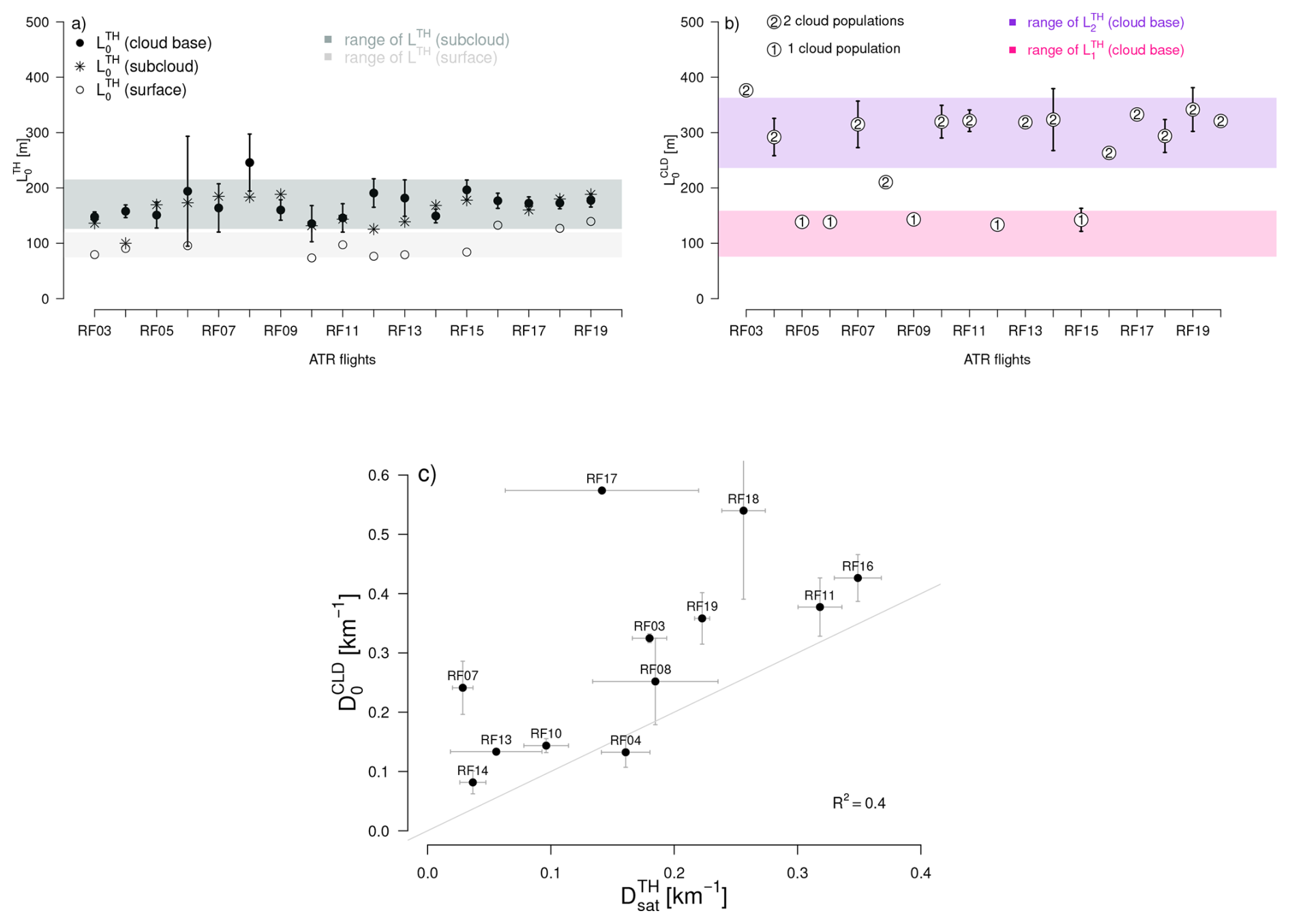
Figure 9 Origin of merged thermals and relationship between thermals and clouds: (a) Length scale of thermals before merging ($L_{\mathrm{0}}^{\mathrm{TH}}$) calculated for each ATR flight near the ocean surface, within the subcloud layer and near cloud base (vertical bars represent the standard error on the mean calculated for each flight on the basis of the repeated flight patterns flown around the cloud base level); $L_{\mathrm{0}}^{\mathrm{TH}}$ values are compared to the range (mean ± standard deviation) of mean thermal lengths ($L^{\mathrm{TH}}=p_{\mathrm{1}}^{\mathrm{TH}}$ $L_{\mathrm{1}}^{\mathrm{TH}}+p_{\mathrm{2}}^{\mathrm{TH}}{L}_{\mathrm{2}}^{\mathrm{TH}}$) measured in the surface layer (light grey) and within the subcloud layer (darker grey). (b) Length scale of clouds before merging ($L_{\mathrm{0}}^{\mathrm{CLD}}$) compared to the range of $L_{\mathrm{1}}^{\mathrm{TH}}$ (pink) and $L_{\mathrm{2}}^{\mathrm{TH}}$ (purple) at cloud base. For each flight, the number reported on the marker indicates whether this flight was associated with one or two cloud populations. $L_{\mathrm{0}}^{\mathrm{CLD}}\approx L_{\mathrm{1}}^{\mathrm{TH}}$ in the presence of a single cloud population, while $L_{\mathrm{0}}^{\mathrm{CLD}}\approx L_{\mathrm{2}}^{\mathrm{TH}}$ in the presence of two cloud populations. (c) Relationship between the density of saturated thermals 𝒟^THsat and the cloud density before merging ${\mathcal{D}}_{\mathrm{0}}^{\mathrm{CLD}}$ (the grey line shows the 1 : 1 line). Saturated thermals may be considered as incipient cloud bases or “cloud shoots”.

Figure 9a shows that in the surface layer, $L_{\mathrm{0}}^{\mathrm{TH}}$ estimates (97 m ± 24 m) are very close to the mean size L^TH of thermals (97 m ± 22 m) and to $L_{\mathrm{1}}^{\mathrm{TH}}$ in that layer (Table 1). It suggests that at that level, thermals experience very little merging and remain largely independent of each other. Within the subcloud layer and near cloud base, on the other hand, $L_{\mathrm{0}}^{\mathrm{TH}}$ estimates (159 ± 27 and 172 ± 26 m, respectively) are close but smaller than the mean thermal sizes found at the same level ($L^{\mathrm{TH}}=\mathrm{170}\pm \mathrm{45}$ m in the subcloud layer and 204 ± 42 m near cloud base). The thermal size distributions measured within the subcloud layer and near cloud base are thus consistent with those expected from the merging of thermals through the depth of the subcloud layer.

Figure 9b shows the $L_{\mathrm{0}}^{\mathrm{CLD}}$ values inferred for each flight from $L_{\mathrm{1}}^{\mathrm{CLD}}$ and $L_{\mathrm{2}}^{\mathrm{CLD}}$ (Fig. 5). In this case, $L_{\mathrm{0}}^{\mathrm{CLD}}$ is bimodal: in the presence of a single cloud population, $L_{\mathrm{0}}^{\mathrm{CLD}}\approx L_{\mathrm{1}}^{\mathrm{TH}}$ (measured near cloud base or in the subcloud layer) $\approx L_{\mathrm{1}}^{\mathrm{THsat}}$, while in the presence of two cloud populations, $L_{\mathrm{0}}^{\mathrm{CLD}}\approx L_{\mathrm{2}}^{\mathrm{TH}}$ (measured near cloud base or in the subcloud layer) $\approx L_{\mathrm{2}}^{\mathrm{THsat}}$ (the close relationship between the thermal length scales and $L_{\mathrm{0}}^{\mathrm{CLD}}$ is further illustrated in Fig. S2). Moreover, the density of clouds prior to merging ${\mathcal{D}}_{\mathrm{0}}^{\mathrm{CLD}}$ correlates well with the density of cloudy thermals 𝒟^THsat (Fig. 9c) or updrafts 𝒟^THup and is of a similar order of magnitude. In fact, ${\mathcal{D}}_{\mathrm{0}}^{\mathrm{CLD}}$ is slightly higher than 𝒟^THsat, suggesting that the merging may involve not only cloudy thermals but also, to a lesser extent, clouds that are not – or no longer – rooted in active thermals.

It thus appears that unmerged thermals that overshoot the LCL form the first population of (very shallow) clouds, and merged thermals that overshoot the LCL generate cloud shoots which, after merging with each other and/or with unmerged saturated thermals, form the second population of clouds, that are on average wider and deeper. The merging of thermals and cloud shoots thus exerts a strong control on the type of clouds present.

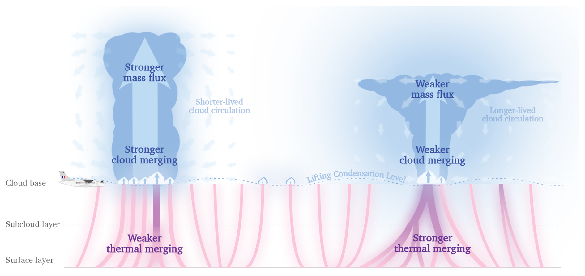
Figure 10 The thermal and cloud merging process (profile view). Each thermal (pink or purple) or cloud (blue) is represented by an updraft. Two objects (thermal or cloud) can merge if they touch each other. However, each convective object exerts an attraction on other objects in its vicinity (shaded area) due to the circulation it creates around itself (Appendix A). Therefore, two objects can merge even without touching if their areas of influence overlap. This makes the merging process more efficient (in the analytic framework, this effect is encapsulated by the effective factor β≥1). Turbulence in the surface layer generates a high density of small thermals that are initially unmerged (pink). These thermals have an exponential size distribution and a mean size $L_{\mathrm{0}}^{\mathrm{TH}}$. As they rise across the depth of the subcloud layer, some of them merge (purple) and become wider. This results in two populations of thermals coexisting in the subcloud layer and near cloud base. The size distribution of these populations can be represented by the sum of two exponentials, each with a characteristic size $L_{\mathrm{1}}^{\mathrm{TH}}\le L_{\mathrm{0}}^{\mathrm{TH}}$ and $L_{\mathrm{2}}^{\mathrm{TH}}\ge L_{\mathrm{0}}^{\mathrm{TH}}$. When the depth of the thermals exceeds the lifting condensation level (whose height varies spatially and tends to be lower in moister areas), incipient cloud bases form (white clouds). The base of these “cloud shoots” has initially the same size as the saturated thermals that produced them ($L_{\mathrm{0}}^{\mathrm{CLD}}\approx L_{\mathrm{1}}^{\mathrm{TH}}\approx L_{\mathrm{1}}^{\mathrm{THsat}}$ or $L_{\mathrm{2}}^{\mathrm{TH}}\approx L_{\mathrm{2}}^{\mathrm{TH}}\approx L_{\mathrm{2}}^{\mathrm{THsat}}$). When cloud shoots form close to each other (which occurs more easily when thermal merging is weak and therefore the thermal density is high around cloud base), they can merge. It forms larger bases (dark blue) and leads to the formation of deeper clouds. The merging process thus leads to a spectrum of clouds whose chord lengths distribution around cloud base can be represented by a sum of two exponentials with characteristic sizes $L_{\mathrm{1}}^{\mathrm{CLD}}$ and $L_{\mathrm{2}}^{\mathrm{CLD}}$. In EUREC⁴A, $L_{\mathrm{1}}^{\mathrm{CLD}}$ is close to the average size of thermals that overshoot the LCL (150–160 m), while $L_{\mathrm{2}}^{\mathrm{CLD}}$ is close to the depth of the subcloud layer on average, but varies strongly with merging conditions.

A schematic of the impact of the merging process on thermals and clouds is represented in the lower half of Fig. 10: turbulence near the surface produces a large density of thermals. As they rise across the depth of the subcloud layer, some of them merge and become wider. This results in two thermal populations coexisting in the subcloud layer and near cloud base: those that have merged (of length scale $L_{\mathrm{2}}^{\mathrm{TH}}$), and those that have not merged yet (of length scale $L_{\mathrm{1}}^{\mathrm{TH}}$). As a result of merging, the thermal density decreases with height. The thermals that overshoot the lifting condensation level (about one out of five on average during EUREC⁴A) saturate at their top and form “cloud shoots” whose base has initially the same size as the saturated thermals that produced them ($L_{\mathrm{0}}^{\mathrm{CLD}}\approx L_{\mathrm{1}}^{\mathrm{TH}}\approx L_{\mathrm{1}}^{\mathrm{THsat}}$ or $L_{\mathrm{0}}^{\mathrm{CLD}}\approx L_{\mathrm{2}}^{\mathrm{TH}}\approx L_{\mathrm{2}}^{\mathrm{THsat}}$, Fig. 9b). As will be shown later (Fig. 12c), a higher density of thermals (𝒟^TH) is associated with a higher density of saturated thermals ${\mathcal{D}}_{\mathrm{sat}}^{\mathrm{TH}}$ (Fig. S5, consistent with the fact that when the density of thermals is high, the boundary layer is moister and the LCL is lower) and thus a higher density of “cloud shoots” (${\mathcal{D}}_{\mathrm{0}}^{\mathrm{CLD}}$, Fig. 9c). When cloud shoots form close to each other (which occurs more easily when thermal merging is weak and thus the thermal density around cloud base is high), they can merge. It forms larger bases and leads to the formation of wider and deeper clouds.

7 Implications of the merging process on clouds and circulations at larger scales

Observations thus reveal a strong relationship between thermal merging and clouds. In this section, we explore its implications for the mesoscale organisation of convection and trade wind cloudiness. During the four weeks of the EUREC⁴A campaign, shallow convection and clouds exhibited a variety of mesoscale organisations and patterns. Based on modeling studies (Bretherton and Blossey, 2017; Narenpitak et al., 2021; Janssens et al., 2023), we expect the transitions between different patterns to be related to the development of shallow mesoscale circulations, which themselves depend on the convective mass flux. We also expect the different patterns of cloudiness to embed different cloud populations (Stevens et al., 2020), and the convective mass flux to influence the cloud fraction near cloud-base (Vogel et al., 2022). Thanks to the repeated flight plan of the ATR during the campaign, we can compare the different flights to each other and shed light on the role of thermal merging in these co-variations.

7.1 Convective mass flux and shallow mesoscale circulations

Each ATR flight was typically associated with two to three hours of in-situ and remote sensing measurements around the cloud base level. During this time, HALO was dropping 3 × 12 dropsondes along three consecutive, 200 km diameter circles (Stevens et al., 2021). From these dropsondes, a horizontal wind divergence and then an area-averaged mesoscale vertical velocity could be estimated (Bony and Stevens, 2019; George et al., 2021, 2023). From the vertical velocity measured around cloud base (W_b) and an analysis of the subcloud layer mass budget (Albright et al., 2022), an area-averaged mass flux M_b could also be estimated (Vogel et al., 2020, 2022). In addition, by using high frequency (25 Hz) in-situ measurements of vertical velocity and humidity from the ATR (Brilouet et al., 2021), we could estimate a linear cloud-base mass flux along the ATR trajectory as $M_{\mathrm{b}}^{\mathrm{ATR}}={\mathrm{\Sigma }}_i{\mathit{\rho }}_i{a}_i{w}_i$, with $a_i=H({\mathrm{rh}}_i-\mathrm{0.98})/N$, where H is the Heaviside function, rh_i and w_i are the relative humidity and vertical velocity (assuming zero mean vertical velocity over each 30 km segment) measured in each point i of the trajectory, N is the total number of measurements made at the cloud base level for each flight, and ρ_i is the air density assumed to be 1 kg m⁻³ for simplicity (see Lamer et al., 2015 for a justification of these approximations).

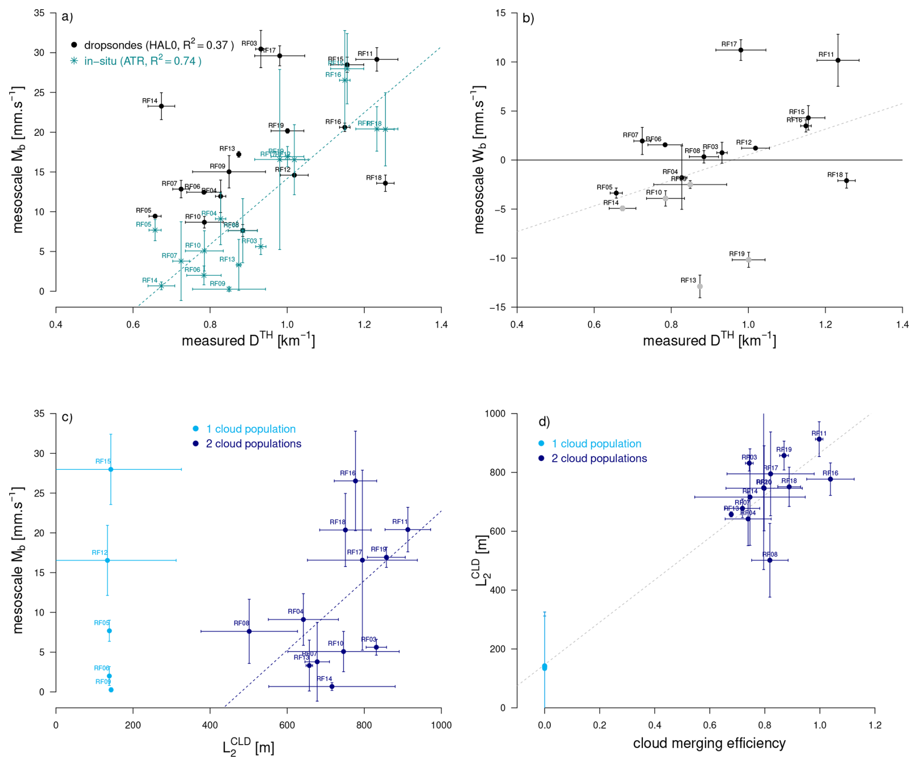
Figure 11 Convective mass flux and shallow mesoscale circulations: Relationship between the thermal density 𝒟^TH measured around cloud base and (a) the domain-averaged mass flux M_b (derived either from dropsondes and the mass budget of the subcloud layer or from in-situ turbulence measurements) and (b) the mesoscale vertical velocity W_b inferred from dropsondes near the cloud-base level (grey markers correspond to the flights whose mixed layer depth suggests that they were influenced by cold pools). (c) Relationship between the cloud lengthscale $L_{\mathrm{2}}^{\mathrm{CLD}}$ and the convective mass flux M_b (note that $L_{\mathrm{2}}^{\mathrm{CLD}}=L_{\mathrm{1}}^{\mathrm{CLD}}$ when only one cloud population is present) and (d) between the cloud lengthscale $L_{\mathrm{2}}^{\mathrm{CLD}}$ and the cloud merging efficiency (defined as ${\left(\frac{L_{\mathrm{2}}-L_{\mathrm{1}}}{\mathrm{2}{L}_{\mathrm{0}}}\right)}^{\mathrm{CLD}}$ or as (β𝒟₀L₀)^CLD). In (c) and (d), all quantities are derived from ATR measurements. In each panel, each point represents one ATR flight. Horizontal and vertical bars represent standard errors on the mean, inferred from the variability of measurements during each flight.

Despite differences during flights where the spatial scale of the cloud organization was larger than the region sampled by the ATR (e.g. RF14), the two independent M_b estimates exhibit the same large flight-to-flight variability, and both correlate positively with the density of thermals near the cloud base level (Fig. 11a). From Vogel et al. (2022) we know that M_b co-varies with the mesoscale vertical motion around cloud base (W_b), and indeed ascending branches of mesoscale circulations (W_b>0) tend to be associated with stronger M_b than subsiding branches (Fig. 11b). We also note that shallow mesoscale circulations tend to be associated with a heterogeneous distribution of thermals, as thermals are more concentrated in regions of mesoscale ascent and low-level convergence and more sparse in regions of low-level divergence. However, the relationship between thermal density and W_b exhibits some outliers. They may be due to the presence of cold pools (e.g. during RF17 and RF18 that were associated with a strong precipitation), which affect the low-level divergence and therefore the measurement of mesoscale vertical motions (Touzé-Peiffer et al., 2022), and likely modulate the distribution of thermals. The relationship between the thermal density inferred from ATR turbulence measurements and the M_b or W_b estimates inferred from HALO dropsondes might also be affected by the different area and time samplings of the two aircraft (e.g. during RF17).

What controls the magnitude of M_b? Since the cloud-base mass flux is known to be more strongly modulated by the cloud size than by the in-cloud vertical velocity (Dawe and Austin, 2012; Vogel et al., 2022), we expect higher values of M_b to be related to the presence of wider clouds. Indeed, when two cloud populations are present, M_b increases with the length scale of the second cloud population (Fig. 11c), which increases with the merging efficiency of clouds (Fig. 11d, Sect. 5). The flight-to-flight variations in M_b can also be interpreted as a result of variations in the thermal population. Noting that M_b can be well approximated by the product of the mean density, length and vertical velocity of cloudy thermals $M_{\mathrm{b}}\approx w_{\mathrm{sat}}^{\mathrm{TH}}\cdot {\mathcal{D}}_{\mathrm{sat}}^{\mathrm{TH}}\cdot L_{\mathrm{sat}}^{\mathrm{TH}}$ (Fig. S6), it appears that M_b variations are primarily governed by ${\mathcal{D}}_{\mathrm{sat}}^{\mathrm{TH}}$ variations (and to a lesser extent by $w_{\mathrm{sat}}^{\mathrm{TH}}$ variations), which are roughly proportional to variations of total density of thermals 𝒟^TH (Fig. S5). In other words, a weaker thermal merging is associated with a higher density of thermals (𝒟^TH) and saturated thermals (${\mathcal{D}}_{\mathrm{sat}}^{\mathrm{TH}}$); this leads to a higher density of cloud shoots (${\mathcal{D}}_{\mathrm{0}}^{\mathrm{CLD}}$, Fig. 9c) and thus promotes cloud merging and the formation of wider cloud bases ($L_{\mathrm{2}}^{\mathrm{CLD}}$ increases), which eventually leads to a stronger mass flux.

However, we note that sometimes a strong mass flux can occur in the absence of cloud merging (Fig. 11c): in RF15 we observe only one cloud population, and the strong mass flux comes from the many small clouds that form on top of a very high density of thermals. In fact, the comparison of RF15 with the following flight (RF16, which occurred a few hours later on the same day) shows that the many small clouds of RF15 later began to merge and form a second population of clouds with wider cloud bases.

What role does the thermal-cloud coupling play in mesoscale circulations? The theoretical study of Janssens et al. (2023, 2024) showed that cumulus mass fluxes favor the development of mesoscale ascents, and the modeling study of Rousseau-Rizzi et al. (2017) showed that the low-level mass convergence associated with mesoscale ascents increases the density of thermals in the subcloud layer. EUREC⁴A observations support these results, but also suggest that a high density of thermals will eventually favor thermal merging, resulting in fewer and wider but more widely spaced thermals. This will reduce cloud merging, and thus M_b, potentially to the point where W_b will become less ascending or even descending. In this way, thermal merging is likely to temper, or act as a negative feedback, on the growth of shallow mesoscale circulations.

7.2 Mesoscale patterns of cloudiness

A large variability of cloud mesoscale patterns was observed during the EUREC⁴A campaign (Schulz, 2022), with the occurrence of each of the four known prominent patterns of tradewind cloudiness (Stevens et al., 2020; Bony et al., 2020). However, most flights were associated with a mixture of cloud mesoscale organizations, and sometimes the ATR was sampling an area smaller than the scale of the cloud pattern itself (e.g. during RF09 the ATR spent most of its flight time in between the cloud systems that constitute the Flower pattern, Bony et al., 2022). In Fig. 12, we highlight the five flights associated with only one cloud population (in green), and six flights (out of 14) associated with two cloud populations and either high or low thermal densities (in orange and red, respectively). An additional flight is highlighted (RF08), which is associated with only one population of (large) thermals (Table 1). The cloud patterns present on these different days are illustrated with satellite images (bottom of Fig. 12). How do they differ in terms of thermal and cloud merging?

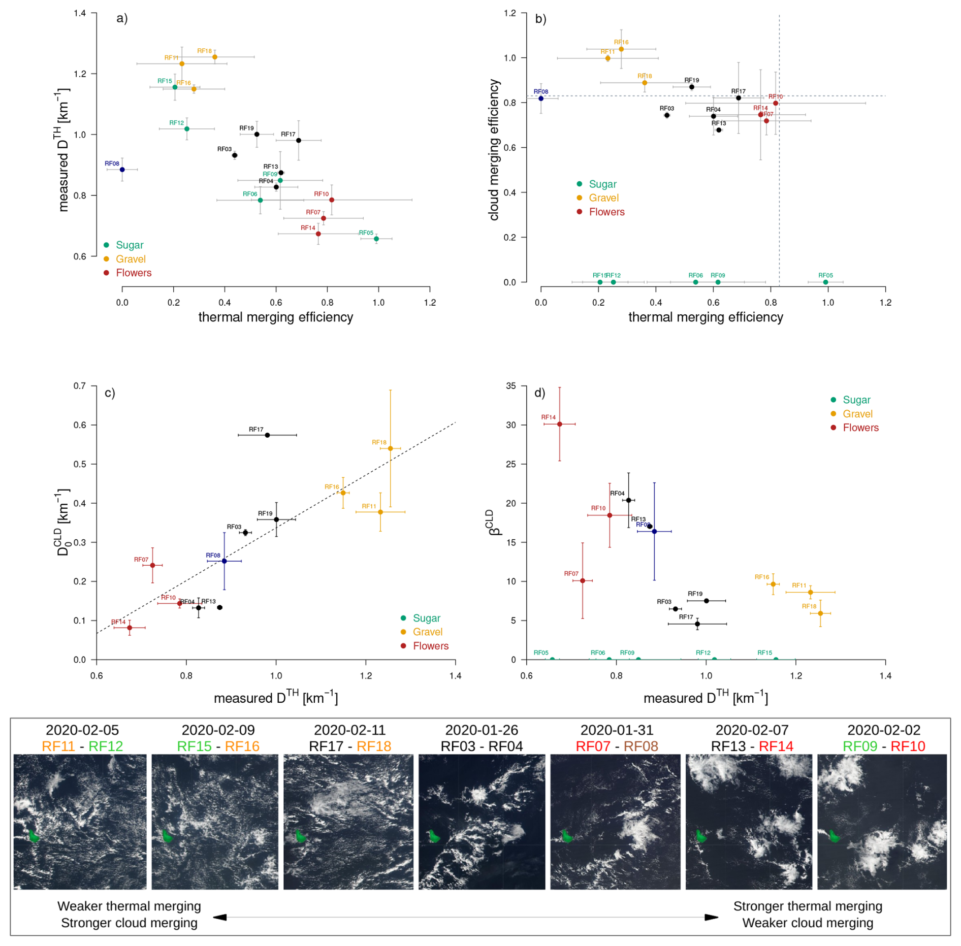
Figure 12 From thermal merging to cloud patterns: Relationship (a) between thermal merging efficiency and thermal density 𝒟^TH (measured near cloud base), (b) between thermal merging efficiency and cloud merging efficiency around cloud base. The dashed line indicates the value of the critical merging efficiency (0.83). A few flights are highlighted, colored as a function of their prominent cloud mesoscale pattern (Sugar, Gravel or Flowers). Panels (c) and (d) show the relationships between the measured thermal density 𝒟^TH and the density of clouds before merging ${\mathcal{D}}_{\mathrm{0}}^{\mathrm{CLD}}$ or the effective length of clouds β^CLD. (bottom) For a few representative flights, illustration of the cloud mesoscale patterns in presence by Suomi-NPP satellite imagery snapshots (at 01:30 p.m. local time) over a domain (57–60° W, 12–15° N) encompassing the EUREC⁴A field of operation (for each date, the corresponding flights are reported). The Barbados island (in green) measures about 20 km × 30 km.

Figure 12a–b show that the measured thermal density is anti-correlated with the strength of thermal merging, and that cloud merging is anti-correlated with thermal merging. These features can be explained as following: when there is little thermal merging, the thermals are small but numerous (𝒟^TH is large), and therefore the cloud shoots rooted in these thermals form close to each other. Since β^CLD>β^TH, the clouds merge more easily than thermals, forming wider cloud bases (Fig. 11d). In contrast, a strong merging of thermals leads to wider but sparser thermals (𝒟^TH is small); the cloud shoots forming on top of these thermals are thus initially wider (because $L_{\mathrm{0}}^{\mathrm{CLD}}=L_{\mathrm{2}}^{\mathrm{TH}}$ and $L_{\mathrm{2}}^{\mathrm{TH}}$ increases with thermal merging) but are more widely spaced and therefore they merge less easily.

Figure 12b suggests that the Gravel pattern corresponds to a minimized thermal merging but maximized cloud merging, and Flowers to a maximized thermal merging and minimal cloud merging. Therefore, when two cloud populations are present: the Gravel pattern maximizes cloud base widths (and in-cloud vertical velocities at cloud base) and thus the convective mass flux, while the Flower patterns minimizes the cloud base widths (and in-cloud vertical velocities) and the convective mass flux (Fig. 11c–d). It is consistent with the observation that the clouds embedded in the Gravel pattern are often deeper and associated with a higher rain rate than those embedded in Flowers (Schulz et al., 2021).

Figure 12a–b show that the situations with only one cloud population (and thus no cloud merging by definition) occur for a wide range of thermal densities and merging efficiencies. The clouds that form in these cases are very small and shallow because they are rooted in small, unmerged thermals (Sect. 6, Fig. 9b). In the absence of other cloud types (such as in RF06), this corresponds to a Sugar pattern (Stevens et al., 2020). However, even in the presence of other cloud types, such clouds are also found because merged and unmerged thermals often co-exist. Therefore, Sugar-like clouds are present in all cloud mesoscale patterns, albeit in a varying proportion that depends on the thermal merging efficiency. When the thermal merging efficiency increases, the effective factor of thermals increases more quickly than their own lengthscale (i.e. β^TH≫1, Fig. 8d). It makes the merging more and more efficient and thus the very shallow clouds more and more sparse. This explains why, in satellite images, the areas between the deepest clouds are less filled with very shallow clouds (and thus appear darker) in the case of Flowers (that are associated with strong thermal merging) than in the case of Gravel (Fig. 12c). It also explains why on a given day associated with a Flower pattern (e.g. on 2 February 2020), the ATR sampled one cloud population on one flight (RF09) when flying in-between the deep clouds, and two cloud populations on the other one (RF10) when flying across the deep clouds.

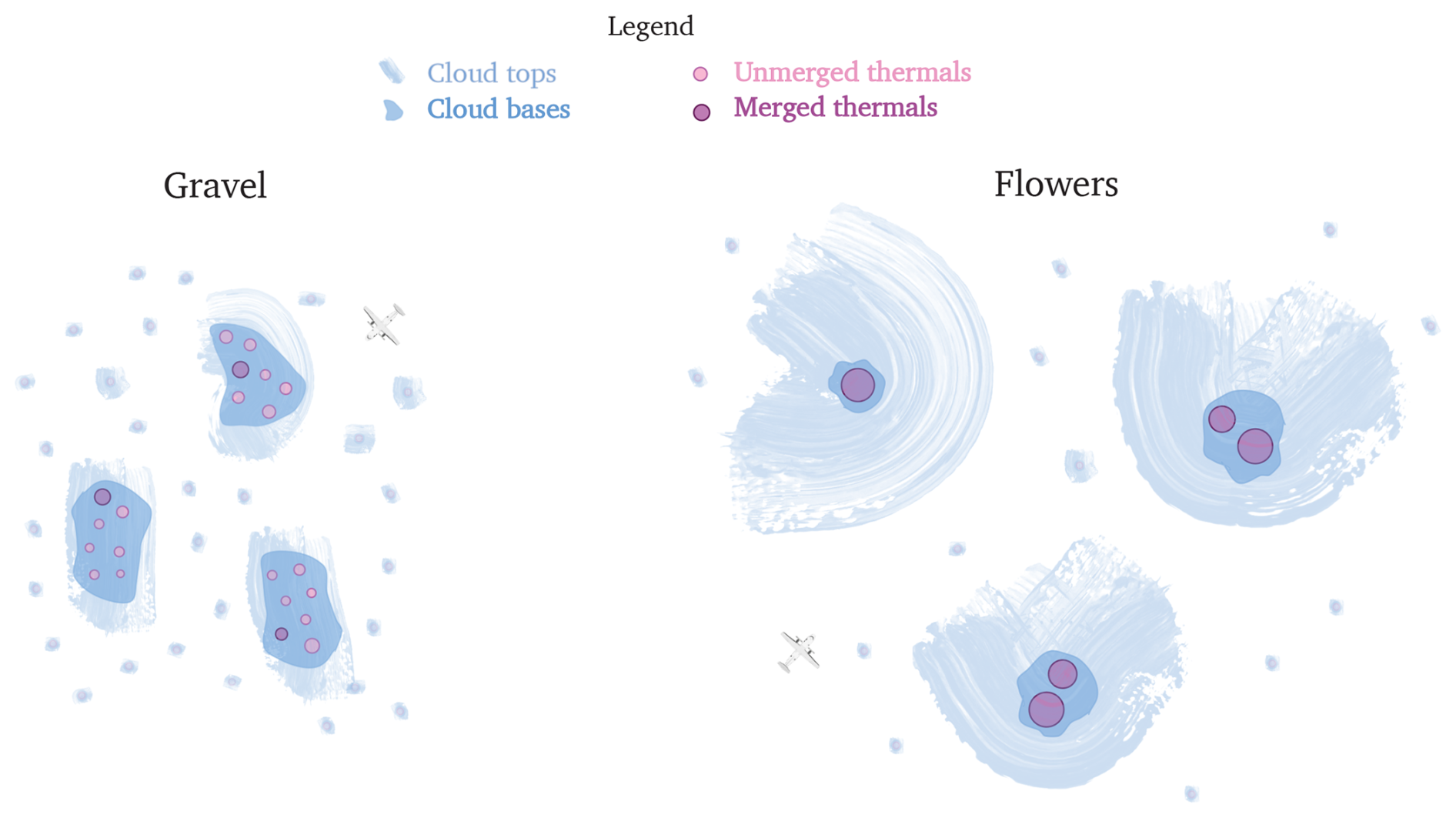
Figure 13 The influence of merging on cloud mesoscale patterns (plan view). When thermal merging is weak (left panel), there are few large thermals around cloud base (purple circles) and a high density of small unmerged thermals (pink circles); the clouds (in blue) that form at the top of the thermals thus merge efficiently, forming large cloud bases (dark blue) and leading to a strong mesoscale mass flux; this situation corresponds to the Gravel mesoscale pattern of cloudiness. When thermal merging is strong (right panel), the thermals widen but their density decreases, so that the thermals are more spaced: the clouds that form at the top of thermals are thus more isolated, which hinders cloud merging. Cloud bases are thus smaller than in the case of Gravel, and the mesoscale mass flux is weaker; on the other hand, clouds are fed by large (merged) thermals, which increases their lifetime and favors the formation of an extended cloudiness around cloud top; this situation corresponds to the Flower type of cloud mesoscale pattern.

Interestingly, we note that the cloud merging efficiency of the different flights (0.85 ± 0.10) is always close to 0.83 (only the Gravel patterns are associated with higher efficiencies). It means that the coupling between thermals and clouds is such that it maximizes the cloud density (Sect. 5 and Fig. 6c). Since the Gravel patterns are associated with a high thermal density but low cloud densities, they are more likely to evolve until the cloud density maximizes, while the Flower patterns (which are fed by wide and longer-lived thermals) are likely to be more stable and persistent. It is consistent with β^CLD, which increases with the lifetime of clouds and is larger for Flowers than for Gravel (Fig 12d).

Vertical and plan views of the interplay between thermals and clouds are represented schematically in Figs. 10 and 13. The left-hand side of the cartoons correspond to a case of weak thermal merging (and thus high thermal density), and the right-hand side to a case of strong thermal merging and low thermal density. The two sides thus correspond to Gravel- and Flowers-types of mesoscale organization, taking into account that the very shallow clouds topping unmerged thermals (represented in the middle of Fig. 10 or around deep clouds in Fig. 13) are also part of these patterns. In the Flower case, deep clouds are represented with an extended cloud coverage at their top (a shallow anvil): it results from the water detrained from the convective core during the lifetime of the convective clouds, which can be particularly long in situations of strong thermal merging and large β^CLD (Fig. 12d, Sect. 6.2).

7.3 Implications for the cloud fraction

The response of trade cumulus clouds to global warming has long been an important contributor to the uncertainty in low-cloud feedback and climate sensitivity (Bony and Dufresne, 2005; Vial et al., 2017). In climate models, this uncertainty is primarily related to changes in cloud fraction near the cloud base level (Brient et al., 2016). EUREC⁴A observations allowed us to show that the climate models that predict the largest trade-cumulus feedbacks overestimate the cloud-base cloud fraction in the current climate, simulate a dependence of this cloud fraction on convection that is at odds with observations, and exhibit difficulties in simulating daily transitions between shallow and deeper trade cumuli (Vogel et al., 2022; Vial et al., 2023). This calls for investigating the influence of the merging process on the cloud fraction near cloud base.

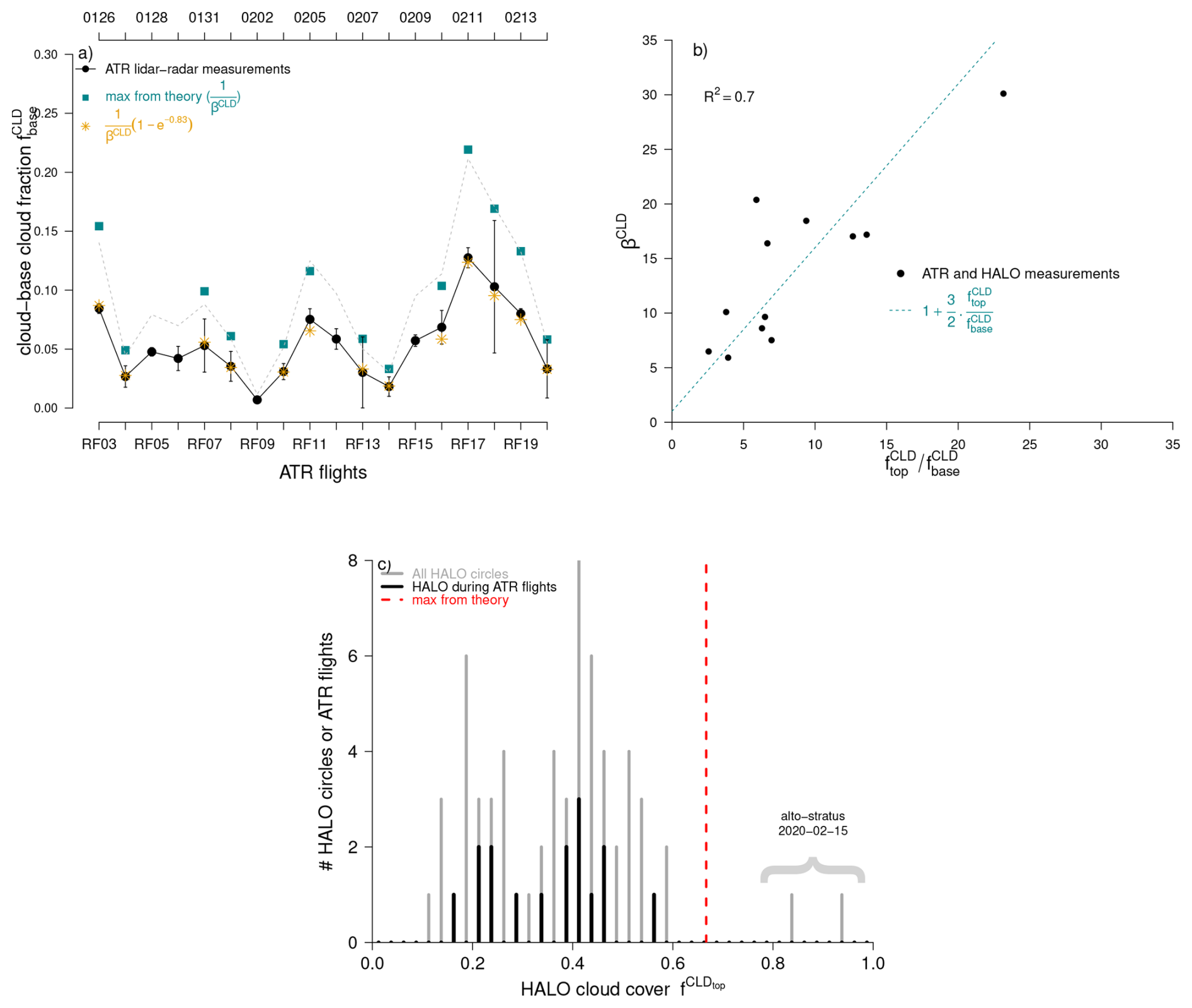
Figure 14 Implications of merging for the cloud fraction at cloud base and cloud top. (a) Evolution of the cloud-base cloud fraction measured from the ATR using horizontal lidar-radar remote sensing (in black, from Bony et al., 2022). Also reported is the maximum cloud fraction predicted by the merging theory ($\mathrm{1}/{\mathit{\beta }}^{\mathrm{CLD}}$, only available when two cloud populations are present) and the cloud fraction estimated from theory when assuming ${\left(\mathit{\beta }{\mathcal{D}}_{\mathrm{0}}{L}_{\mathrm{0}}\right)}^{\mathrm{CLD}}$ = 0.83. (b) Relationship between β^CLD (inferred from cloud-base measurements as explained in Sect. 5) and the ratio between the cloud cover measured from above by HALO ($f_{\mathrm{top}}^{\mathrm{CLD}}$ and the cloud fraction measured at cloud base by the ATR ($f_{\mathrm{base}}^{\mathrm{CLD}}$). (c) Histogram of the cloud cover measured from the upper troposphere by HALO using downward-looking lidar-radar remote sensing and radiometers. Data from all HALO circles performed during EUREC⁴A are shown in grey (from Konow et al. (2021). HALO measurements performed during the ATR flights are shown in black. The red line shows the upper bound ($\mathrm{2}/\mathrm{3}$) on $f_{\mathrm{top}}^{\mathrm{CLD}}$ estimated from theory. The only measurements exceeding this value were made on Feb 15th 2020, when HALO was flying above a persistent layer of altostratus independent of boundary-layer processes.

As discussed in Sect. 5, the final coverage of merging objects depends on their merging efficiency and β. According to Eq. (12), the coverage increases as the initial density 𝒟₀ or size L₀ increases, but it is bounded by the maximum value $f_{max}=\mathrm{1}/\mathit{\beta }$. Therefore, for a given merging efficiency, the final coverage decreases as β increases. During EUREC⁴A, β^CLD≥5 (Fig. 12d) and therefore 0.2 appears to be an upper bound for the cloud fraction around cloud base. Furthermore, since $\mathit{\beta }{\mathcal{D}}_{\mathrm{0}}{L}_{\mathrm{0}}^{\mathrm{CLD}}$ is never far from 0.83 (Fig. 12b), the cloud base cloud fraction is well approximated by $(\mathrm{1}-e^{-\mathrm{0.83}})/{\mathit{\beta }}^{\mathrm{CLD}}$ (Fig. 14a). It highlights the important role of β^CLD in modulating, and limiting, the cloud fraction around cloud base.

As discussed in Sect. 6.2 and Appendix A, simple physical arguments suggest that β encapsulates the influence that the circulation produced by convective objects exerts on neighbouring objects. Then, how to physically interpret the fact that β^CLD constrains the cloud fraction? The f_max limit corresponds to the maximum cloud fraction for which the clouds' basins of attraction remain non-overlapping. In a cloud field with an area fraction $\mathrm{1}/{\mathit{\beta }}^{\mathrm{CLD}}$, then any new clouds born in the domain would necessarily be within an existing cloud's “basin of attraction” and would therefore merge with that cloud (in the simplest case where β^CLD=1, a new cloud born in a region with a cloud fraction of unity would necessarily imply overlap and merging with existing clouds and no further increase in cloud fraction). Another interpretation is that the circulation induced by clouds likely promotes a mass convergence around their base level that favors the merging of thermals and thus decreases the cloud base fraction (Fig. 10).

Moreover, the circulation induced by clouds facilitates the merging process all the more that the clouds live longer. How may thermal merging influence the cloud lifetime? When thermal merging increases, the thermals become wider, and therefore they are more likely associated with positive buoyancy and stronger vertical velocities (Böing et al., 2012; Rochetin et al., 2014; Morrison et al., 2022), and thus with stronger circulations. Clouds are likely to live longer when they are fed by such active thermals, and therefore associated with a larger β^CLD.

Consistently, the situations with weak thermal merging, that predominantly correspond to the Gravel type of organization (Sect. 7.2), are associated with short-lived clouds, β^CLD values ranging from 6 to 10 and a measured cloud fraction that ranges from 0.07 to 0.1 at cloud base. In contrast, the situations with strong thermal merging, that correspond to Flowers, embbed clouds that have much longer lifetimes (as shown by Narenpitak et al. (2021), on 2 February 2020 the cloud flowers followed along their Lagrangian trajectory seemed almost motionless for more than 12 h), β^CLD ranges from 10 to 30 and the cloud base cloud fraction does not exceed 0.05. By enhancing the lifetime of clouds, thermal merging thus exerts a strong control on the cloud-base cloud fraction.

As explained in Sect. 6.2, β^CLD can also be related to the aspect ratio of clouds, i.e. the ratio between cloud length scales at cloud top and at cloud base: $\mathit{\beta }=\mathrm{1}+\mathit{\gamma }\frac{f_{\mathrm{top}}^{\mathrm{CLD}}}{f_{\mathrm{base}}^{\mathrm{CLD}}}$, where $\mathit{\gamma }=h^{\prime }/h$ is the ratio between the outflow and inflow layer depths of the air transported by the cloud circulation. Since $f_{\mathrm{base}}^{\mathrm{CLD}}$ is bounded by $\mathrm{1}/{\mathit{\beta }}^{\mathrm{CLD}}$, the cloud cover measured from top is also bounded by $\frac{\mathrm{1}}{\mathit{\gamma }}(\mathrm{1}-\mathrm{1}/{\mathit{\beta }}^{\mathrm{CLD}})$. Figure 14b shows the relationship between β^CLD (inferred from ATR measurements as explained in Sect. 5) and the ratio $\frac{f_{\mathrm{top}}^{\mathrm{CLD}}}{f_{\mathrm{base}}^{\mathrm{CLD}}}$, using $f_{\mathrm{top}}^{\mathrm{CLD}}$ measurements from the downward-looking instruments on board HALO (Konow et al., 2021).

Indeed, the two quantities are actually strongly correlated (Pearson correlation equals 0.84), and the relationship is reasonably reproduced using $\mathit{\gamma }=\mathrm{3}/\mathrm{2}$, supporting our hypothesis that the effective factor β^CLD arises from the presence of cloud-induced circulations. We thus expect $f_{\mathrm{top}}^{\mathrm{CLD}}$ to be bounded by $\mathrm{1}/\mathit{\gamma }=\mathrm{2}/\mathrm{3}$. The histogram of $f_{\mathrm{top}}^{\mathrm{CLD}}$ values inferred from HALO measurements (considering the maximum cloud fraction estimates across the different instruments) during the whole EUREC⁴A field campaign shows that this value actually represents an upper bound for the measurements (Fig. 14c). Over the 86 circles flown by HALO during January–February 2020, the cloud fraction exceeded this value only twice, on 15 February 2020, when HALO was flying above a persistent layer of altostratus that has no reason to depend on boundary layer processes and thermal merging.

8 Conclusion and discussion

In line with early studies of atmospheric convection (Simpson et al., 1965; Ooyama, 1971; Arakawa and Schubert, 1974; LeMone and Pennell, 1976; Lenschow and Stephens, 1980; Williams and Hacker, 1993), this study emphasizes the importance of the thermal-cloud interplay in convection dynamics, and confirms its imprint on the statistical distribution of cloud-base widths. It goes further by showing the central role of the merging process in facilitating this interplay and the constraints it imposes on the mesoscale organization of convection and the cloud fraction.

8.1 Summary of main findings

These findings are the result of analyzing and interpreting the interplay between thermals, clouds, mesoscale circulations and cloud patterns that was observed over the tropical Atlantic Ocean during the EUREC⁴A field campaign. During the campaign, the atmosphere was statistically sampled over a four-week period with two research aircraft that followed a repeated flight pattern. The ATR aircraft flying in the lower troposphere characterized boundary-layer thermal and cloud base chords using high-frequency humidity measurements and horizontal lidar-radar remote sensing while the HALO aircraft observed clouds from above and measured mesoscale circulations using dropsondes.

Airborne observations taken at several heights throughout the subcloud layer show that the density of thermal chords decreases with height while their average size increases. The observations also reveal that the distribution of thermal chord lengths is exponential in the surface layer, and that it is well fitted by a sum of two exponential functions higher up in the subcloud layer and near cloud base. Measurements of cloud chord lengths around the cloud base level also exhibit two populations of chords. Similar to thermals, the size distribution of cloud chords is well fitted by a sum of two exponentials, when considering either the whole campaign or individual flights. The length scale of the first cloud exponential is similar to the average size of individual thermals, while the length scale of the second cloud exponential is several times larger. Then, the detailed analysis and interpretation of these observations addresses three main questions: (1) What physical process explains the double exponential distributions? (2) How do the thermal and cloud size distributions relate to each other? (3) How do these distributions inform our physical understanding of the mesoscale organization of convection?

Physical insight and mathematical calculations, supported by simple statistical simulations, show that the merging of objects with initially exponentially distributed chord lengths leads to a sum of two exponential distributions. One exponential corresponds to objects that have merged, and the other corresponds to objects that have not yet merged. Furthermore, physical arguments suggest that the circulation created by convective objects influences the surrounding objects in a way that facilitates the merging process. This influence is formally similar to assuming that the objects have an effective length greater (by a factor β, the effective factor) than their actual length. The merging efficiency and effective factor of objects can be inferred from their chord length distribution and total coverage after merging.

Based on this conceptual framework, we diagnose the merging efficiency and effective factor of thermals and clouds using EUREC⁴A observations, and we predict the thermal density that results from the merging process. The good agreement between this prediction and the measured thermal density (which was not used to infer the merging diagnostics) provides an independent test of the consistency between the theory and the observations. We then analyze the ensemble of EUREC⁴A observations in the light of this interpretation framework.

This analysis suggests that the thermals formed in the surface layer progressively merge as they rise through the subcloud layer. This decreases the thermal density and creates two populations: one of small, unmerged thermals averaging 100–120 m, and another of larger thermals averaging about 300 m. The cloud chord length distributions are closely related to these thermal populations (Fig. 10). Merged and unmerged thermals constitute the roots of cloud-base widths: upon reaching the LCL, they saturate and give rise to cloud shoots (incipient cloud bases) which in turn merge and produce two cloud populations. The clouds that results from unmerged cloud shoots are horizontally small (they have roughly the same size as individual thermals), very shallow and non drizzling. On the other hand, the clouds that result from merged cloud shoots have a wider base, develop deeper and produce drizzle. The circulation they create around them (encapsulated by the effective factor) is also stronger, which likely reinforces the concentration and merging of underlying thermals, and reduces the presence of very shallow clouds in their vicinity. The interplay between thermals and clouds, combined with the merging process, has several significant implications.

First, the merging efficiencies of thermals and clouds are negatively correlated: when thermal merging is weak, the thermal density is high, which results in a high density of cloud shoots. This facilitates cloud merging, forms large cloud bases, increases the mesoscale mass flux and strengthens mesoscale circulations. However, the convergence of thermals below large clouds eventually strengthens thermal merging, which produces wider but more isolated thermals and a lower density of cloud shoots. This hinders cloud merging and reduces the mesoscale mass flux. The interplay between thermal and cloud merging thus represents a negative feedback on the growth of mesoscale circulations, thus regulating the intrinsically unstable growth of shallow mesoscale circulations (Janssens et al., 2023).

Second, we observe a correspondence between the degree of thermal merging and the type of prominent mesoscale cloud pattern: situations of weak thermal merging tend to be associated with Gravel-type organization, while situations of strong thermal merging tend to be associated with Flower patterns. On the other hand, the very shallow clouds that cap single thermals can be found in all situations, either alone (thus forming a Sugar-type organization) or in association with other cloud types. Moreover, since cloud merging promotes the formation of larger cloud bases, deeper clouds and stronger mass fluxes, it contributes to the development of the shallow mesoscale circulations that have been shown to accompany the transitions from Sugar-Gravel to Flower types of organization in Large-Eddy Simulations (Narenpitak et al., 2021). The analysis of these simulations, that will be presented in a separate paper, confirms this inferrence.

Finally, physical arguments suggest that the maximum cloud fraction that can be achieved at cloud base is inversely proportional to the cloud effective factor, which depends on the cloud lifetime. Since clouds presumably live longer when they are fed by wide, isolated thermals than when they are fed by small thermals, thermal merging reduces the cloud fraction near cloud base. This is consistent with the minimal cloud fraction measured at cloud base in Flower-type organizations, and with the positive relationship between cloud fraction and mesoscale mass flux pointed out by Vogel et al. (2022). Physical arguments also suggest that the cloud top coverage is limited by the lifetime of clouds, and EUREC⁴A measurements are consistent with this suggestion.

8.2 Open questions and perspectives

A number of observed features remain to be interpreted. For instance, a surprising observation is that the cloud merging efficiency is never far from 0.83 (Fig. 12b), which is the theoretical value that maximizes the cloud density after merging (Fig. 6). Whether or not this is a general feature constrained by some physical process remains to be understood. Another interesting feature is the underestimate, compared to observations, of the thermal density predicted by theory in situations of maximal thermal merging or minimal thermal density after merging (Fig. 8a). This discrepancy suggests the influence of additional processes in the control of the thermal density. These processes might include the influence of mesoscale circulations, which concentrate thermals in ascending branches (as shown by Fig. 11b at the scale of a 200 km circle), or the presence of cold pools, which may concentrate thermals and thus favor thermal merging at their edge. The discrepancy may also result from the mass convergence induced by clouds in the subcloud layer, which may influence the distribution of thermals beneath clouds and thus thermal merging but is not adequately accounted for by the effective factor of thermals (because it arises from clouds). These influences will need to be studied. Finally, the sensitivity of thermal merging to factors such as the strength of surface turbulent fluxes, the Bowen ratio or environmental conditions, and the sensitivity of cloud merging to humidity and wind shear will have to be investigated.

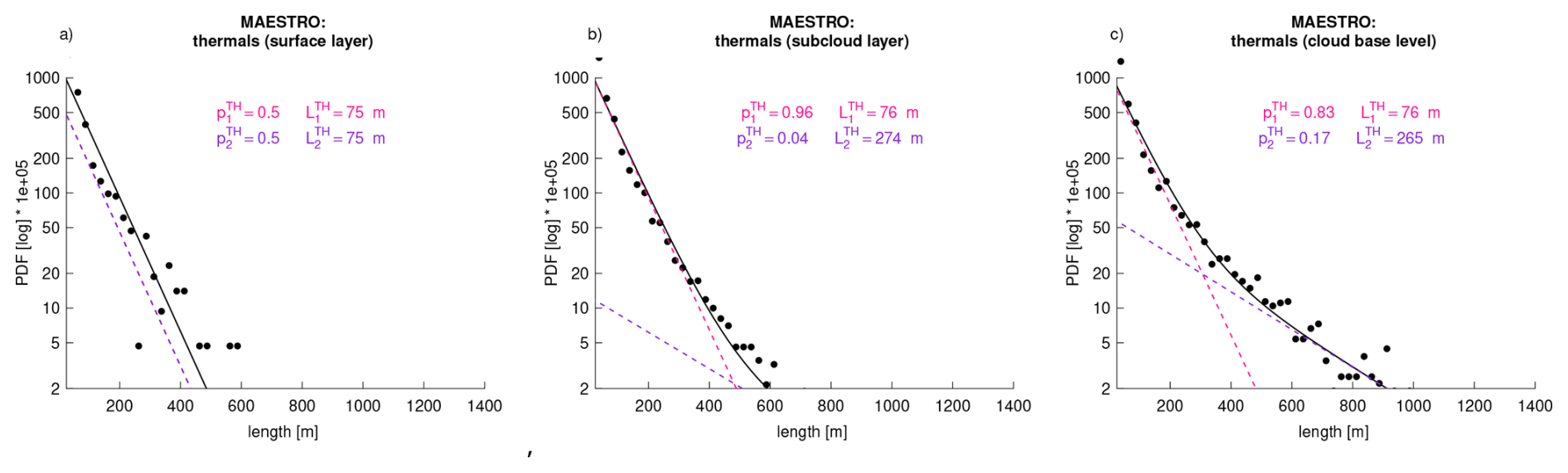
Figure 15 Universality of the thermal chord distributions? Same as Fig. 1 but for measurements from the Mesoscale Organisation of Tropical Convection (MAESTRO) field campaign that took place on August–September 2024 around Cape Verde in regimes of shallow to deep convection.

More importantly, this study emphasizes the role of thermal- and cloud-induced circulations in shaping mesoscale organization and cloud patterns. Within the analysis framework presented here, these circulations are conceptualized by the effective factor β, which quantifies the basin of attraction exerted by a convective object on its surroundings and influences the merging process as if convective objects had an effective size β times their actual size. The factors that influence β remain to be clarified. For instance, how should we interpret the fact that inter-flight variability of β^TH is larger than its intra-flight variability (Fig. 8d)? A deeper investigation into the dependence of β on convective object properties and environmental conditions would help answer this question. In addition, this study shows the role of merging in shaping the size distribution of thermals and clouds, but does not show how exactly the merging – or the contact between two adjacent objects – actually occurs. The influence on the size, orientation and movement of rising thermals and clouds, and consequently on merging efficiency, of processes such as entrainment at thermal and cloud edges, ambient horizontal flow or wind shear, or buoyancy-induced pressure gradients, should be further investigated with additional observations and/or simulations.

The findings of this study offer new opportunities to understand and predict the mesoscale organization of convection, as well as its role in climate.

Given the importance of the transition between shallow and deeper trade cumuli in cloud feedback (Vial et al., 2023), and the uncertainty surrounding the role of cloud mesoscale organization in climate sensitivity (Bony et al., 2015; Nuijens and Siebesma, 2019; Becker and Wing, 2020; Alinaghi et al., 2024), it will be important to verify that the models used to study convective organization and cloud feedbacks realistically represent this essential piece of atmospheric physics. By relating the statistical distribution of thermal and cloud chords to the processes that control the cloud's geometry, convective mass fluxes and mesoscale circulations, this study paves the way towards a better interpretation of the ability of numerical models to predict the different forms of mesoscale convective organization: Why do Large Eddy Simulation (LES) models or Cloud Resolving Models exhibit more success or difficulty predicting Flower-type of organization than Gravel? Why do they predict clouds that may be too scattered or on the contrary excessively wide, deep and clustered? How does the representation of thermal merging and the thermal-cloud interplay depend on the spatial resolution of models? These questions may be addressed through model inter-comparisons such as EUREC⁴A-MIP (https://eurec4a.eu/mip, last access: 14 June 2025) or large ensembles of simulations such as the Cloud Botany dataset (Jansson et al., 2023). Analyzing these simulations would also allow us to investigate how environmental conditions influence thermal merging, which will advance understanding of how the mesoscale convective organization might respond to climate change.

In turn, the conceptualization of thermal and cloud populations as a mixture of two populations that interact and evolve through merging could help develop conceptual models that aim at representing the spectrum of cumulus clouds, their dynamics and their mesoscale organization. Such conceptual models could also be used to parameterize the mesoscale organization of convection in coarse general circulation models. With the exception of Rochetin et al. (2014), pioneering studies in this direction have often described the statistical distribution of cloud base widths using power laws or other heavy-tail distribution functions (Sakradzija et al., 2015; Neggers, 2015; Neggers and Griewank, 2022). Studies also noticed the frequent presence of a scale break dependent on the spatial organization of convection (e.g., Neggers and Griewank, 2022), and Savre and Craig (2023) suggested that the merging of cloud cores could influence the scale behavior of the cloud size distributions. The mathematical arguments presented in Sect. 5 suggest that a double exponential would be a more natural description of these distributions. It will need to be confirmed.

Finally, since EUREC⁴A took place in a regime of shallow convection, the question arises as to whether the findings of this study are specific to shallow convection, or could apply to a broader range of convective regimes. Exponential distributions of updraft chord lengths and mass fluxes have been pointed out in various contexts, ranging from observations of cloud-free continental convection (Miao et al., 2006) to idealized simulations of deep convection (Cohen and Craig, 2006). It remains to be clarified whether the absence of a second exponential may be due to the absence of merging (as may occur in simulations without mesoscale organization), and/or to a spatial resolution of simulations or observations that is too coarse to detect the smallest thermals or clouds. In any event, several elements suggest a certain universality of our results. First, the mathematical calculations and simple statistical simulations presented in Sect. 5 are not specific to shallow convection and would apply equally to deep convection. Second, the interplay between thermals and clouds that has been characterized here for different organizations of shallow clouds resembles that at work during the transition from shallow to deep convection over land or ocean (Grabowski et al., 2006; Kuang and Bretherton, 2006; Böing et al., 2012; Rochetin et al., 2014; Morrison et al., 2022), including in the presence of mesoscale circulations (Rousseau-Rizzi et al., 2017). However, this important question deserves further investigation.

Another question to be addressed is how much the merging process contributes to the self-organization of convection. Thermal merging has been suggested to play a role in the inverse energy cascade from the smaller to larger scales (Zilitinkevich et al., 2021). In addition, modelling studies suggest that cold pools or radiatively-driven circulations are not necessary to organize shallow convection (Bretherton and Blossey, 2017; Janssens et al., 2023), and this is consistent with our results. Whether the merging process can also lead to the spontaneous organization of deep convection, and should be added to the list of physical processes that have already been identified (Muller et al., 2022), will have to be explored.

The recent MAESTRO (Mesoscale organisation of tropical convection, https://maestro.aeris-data.fr, last access: 14 June 2025) field campaign, which took place in August–September 2024 near Cape Verde as part of ORCESTRA (Organized Convection and EarthCARE Studies over the Tropical Atlantic, https://orcestra-campaign.org, last access: 14 June 2025), is an opportunity to explore the universality of the merging process across convective regimes. During MAESTRO, the ATR measured again humidity at a fast rate at different levels of the subcloud layer and at cloud base, in a wide range of meteorological situations ranging from shallow to deep convection (Jaffeux and Lothon, 2025; Jaffeux et al., 2025). Using the same methodology as described in Sect. 3, we analyzed the thermals sampled during this campaign. Figure 15 shows that the thermal chord length distributions derived from MAESTRO observations resemble those from EUREC⁴A, further supporting the idea of a certain universality in the processes revealed by EUREC⁴A observations. However, further studies will be needed to confirm this conclusion, and to investigate how the interplay between thermal, clouds and circulations varies across a large diversity of convective organizations.

Finally, this study emphasizes the importance of considering the circulations induced by convective objects to understand the mesoscale organization of convection. This insight harkens back to a school of thought considering convective objects not just as thermodynamic entities (e.g. Arakawa and Schubert, 1974) but also as geometric and dynamic entities (e.g. Bretherton, 1987; Neggers, 2015; Poujol, 2025). As fine-scale atmospheric models are now being used on large domains and multi-scale observations of convection, such as those from EUREC⁴A or ORCESTRA, are becoming available, a more complete understanding of the dynamical nature of thermal and clouds, and its implications for mesoscale oganization, is not only becoming warranted, but also possible.

Appendix A: Effective length of convective objects

In this section, we aim at providing an explanation for the merging process of convective objects, and deriving a simple merging criterion based on basic properties of the convective objects.

Let us consider two updrafts, such as clouds or thermals. These updrafts can merge if they touch each other, as represented in Fig. A1a. However, we can also consider that if the updrafts are close enough, they can merge by attracting each other through the circulations they create (Fig. A1b). This process is illustrated on Fig. A2, that sketches the resulting circulation implied by two convective objects, at the moment the objects are created. Assuming that the position of the updrafts is controlled by their base (where the warm bubbles are formed), the two updrafts attract each other as indicated by the red arrows. To account for this process, let us note by T_life the lifetime of an updraft. Two updrafts will merge if they have the time to attract each other until merging before they die.

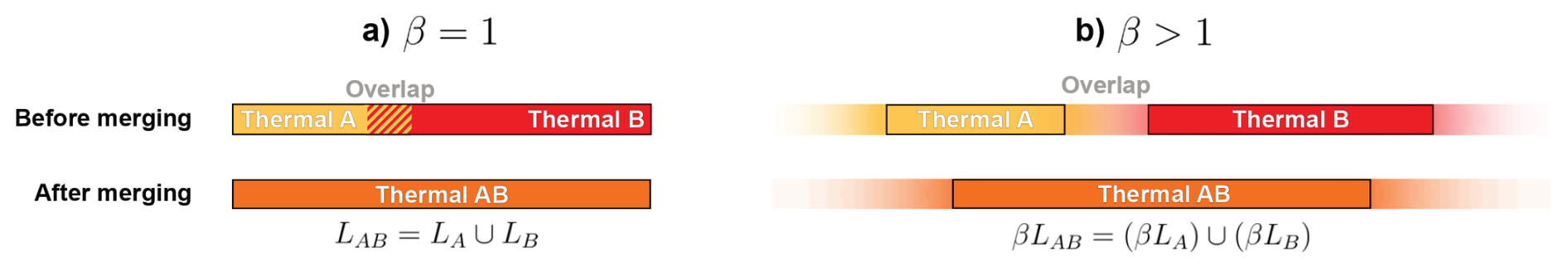
Figure A1 Illustration of the merging process assuming two objects merge (a) if and only if they overlap or (b) if their basins of attraction overlap – the basin of attraction (or effective length) of object A has a length βL_A, where L_A is the actual length of object A and β is the effective factor (shown in shading, defined in Appendix A and further interpreted in Sect. 6.2). The rules for object merging are as follows. When β=1, the length of the merged (L_AB) object will be the union of the two incipient objects' lengths (L_A∪L_B). When β>1, the length of the merged object's basin of attraction (βL_AB) will be the union of the two incipient objects' basins of attraction (βL_A∪βL_B).

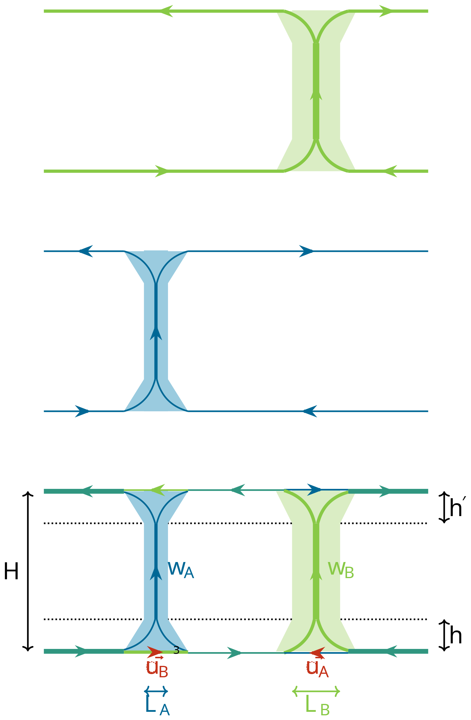
Figure A2 The circulation created by two updrafts, as well as the resulting circulation. The red arrows highlight the advection experienced by the base of each updraft, and indicate the attraction between the two updrafts. H, h and h^′ are the depths of the updraft and of the inflow and outflow layers, respectively. u_A and u_B are the horizontal winds induced by updrafts A and B, respectively.

We aim at computing the time needed for two updrafts to merge. We first consider an updraft (updraft A; in blue on the schematic) that has a depth H, a width L_A, and a vertical velocity w_A. The horizontal wind u_A created by updraft A can be computed by mass conservation. Assuming that the updraft is fed by an inflow layer of depth h then mass conservation implies that w_AL_A=2u_Ah, which directly provides an estimate for u_A. Let us now consider a second updraft (updraft B) that is located at a distance ℓ from updraft A. We first assume that updraft B is passive for simplicity. The time necessary for two updrafts to merge is given by:

$$\begin{array}{}\text{(A1)}& T_{\mathrm{merge}}\left(\mathrm{\ell }\right)={\displaystyle \frac{\mathrm{\ell }}{u_{\mathrm{A}}}}=\mathrm{2}{\displaystyle \frac{h\mathrm{\ell }}{w_{\mathrm{A}}{L}_{\mathrm{A}}}}\end{array}$$

To improve the physical interpretation of the expression, we define the transit time of the updraft:

$$\begin{array}{}\text{(A2)}& T_{\mathrm{transit}}={\displaystyle \frac{H}{w_{\mathrm{A}}}}\end{array}$$

which is the time necessary for an air parcel to travel from the bottom to the top of the updraft.

The merging will occur if, and only if, T_merge≤T_life. This translates into a maximum distance between the edges of the two updrafts for merging to occur:

$$\begin{array}{}\text{(A3)}& {\mathrm{\ell }}_{\max ,\mathrm{A}}={\displaystyle \frac{L_{\mathrm{A}}}{\mathrm{2}}}{\displaystyle \frac{H}{h}}{\displaystyle \frac{T_{\mathrm{life}}}{T_{\mathrm{transit}}}}\end{array}$$

Up to this point, we have considered that updraft B was passive. However, it also exerts an attracting force on updraft A and the real maximal distance for the merging between the two updrafts is given by:

$$\begin{array}{}\text{(A4)}& {\mathrm{\ell }}_{\max ,\mathrm{A}+\mathrm{B}}={\mathrm{\ell }}_{\max ,\mathrm{A}}+{\mathrm{\ell }}_{\max ,\mathrm{B}}={\displaystyle \frac{L_{\mathrm{A}}+L_{\mathrm{B}}}{\mathrm{2}}}{\displaystyle \frac{H}{h}}{\displaystyle \frac{T_{\mathrm{life}}}{T_{\mathrm{transit}}}}\end{array}$$

and therefore merging will occur if the centers of the two updrafts are separated by less than:

$$\begin{array}{}\text{(A5)}& {\displaystyle \frac{L_{\mathrm{A}}+L_{\mathrm{B}}}{\mathrm{2}}}+{\mathrm{\ell }}_{\max ,\mathrm{A}+\mathrm{B}}={\displaystyle \frac{L_{\mathrm{A}}+L_{\mathrm{B}}}{\mathrm{2}}}\left(\mathrm{1}+{\displaystyle \frac{H}{h}}{\displaystyle \frac{T_{\mathrm{life}}}{T_{\mathrm{transit}}}}\right).\end{array}$$

Then, everything happens as if the updrafts need to overlap to merge, but having a length multiplied by an effective factor β:

$$\begin{array}{}\text{(A6)}& \mathit{\beta }=\mathrm{1}+{\displaystyle \frac{H}{h}}{\displaystyle \frac{T_{\mathrm{life}}}{T_{\mathrm{transit}}}}\end{array}$$

In other words, taking into account the influence of the thermal-induced circulations on merging amounts to replace the actual updrafts by effective objects whose size is the actual size of the updrafts multipled by β.

The effective updrafts have their size multiplied by β, and they merge if and only if they actually touch. As a result, we can consider a population of effective updrafts, that have a characteristic size βL₀ and a density 𝒟₀, and we want to study the efficiency of the merging process between those effective updrafts. The merging between those effective updrafts acts as shown on Fig. A1. After merging, it is straightforward to come back to the size distribution of real updrafts, by dividing again the size of the effective updrafts by the factor β.