German methane fluxes estimated top-down using ICON–ART – Part 2: Inversion results for 2021

A reliable quantification of greenhouse gas emissions is important for climate change mitigation strategies. Inverse methods based on observations and atmospheric transport simulations can support emission quantification at the national scale, yet, they are often limited by the observing systems, transport model uncertainties, and inversion methodologies. This two-part study introduces a system for observation-based, regional methane flux estimation. In the present Part 2, we apply this system to estimate German methane emissions in 2021. The numerical weather prediction model ICON with its ART module for trace gases is used to simulate the atmospheric transport while estimating uncertainties using a transport ensemble. We use a priori fluxes from national reporting to facilitate the validation of reported fluxes. Posterior fluxes are estimated with a modified synthesis inversion method introduced in Part 1, relying on in-situ observations. Compared to the a priori, we find a significant increase in methane emissions in Germany and in the Benelux. We estimate German methane emissions (32±19) % higher than the anthropogenic emissions in the national inventory, and our inversion method attributes this difference mainly to the agricultural sector, although separation from Land Use, Land Use Change and Forestry (LULUCF) as well as natural fluxes requires further research. The combination of an ensemble-enhanced numerical weather prediction model for atmospheric transport and good observation coverage paves the way to sector-specific, observation-based national emission estimates.

1 Introduction

Reducing greenhouse gas (GHG) emissions is crucial for mitigating current anthropogenic global warming. UNFCCC (United Nations Framework Convention on Climate Change) compliant national inventories and/or process models quantify anthropogenic GHG emissions for the purpose of monitoring the effectiveness of mitigation as planned, e.g., in the Paris Agreement. In addition to so-called “bottom-up” methods, atmospheric GHG concentration observations are used in “top-down” flux estimations. The latter are complementary, as they are sensitive to the total fluxes (i.e., anthropogenic and natural) and provide options for independent validation of a priori fluxes provided by inventories (IPCC et al., 2019). The usefulness of top-down estimates has been demonstrated, e.g., for the United Kingdom (Manning et al., 2011), Switzerland (Henne et al., 2016), Europe (Petrescu et al., 2023) and globally (Deng et al., 2022; Petrescu et al., 2024).

Although research foundations for top-down methods have been developed in recent decades (see Janssens-Maenhout et al., 2020, and references therein), applications remain limited due to sparse observation coverage and representativeness, and most critically, due to transport model uncertainties (Engelen et al., 2002; Gerbig et al., 2008). The latter is a well-known issue not solved yet (Munassar et al., 2023). Inversions using satellite observations (e.g. Estrada et al., 2025) benefit from larger spatial observation coverage, but the uncertainties of the observations are larger compared to in situ data and the influence on the inversion results was found smaller where in situ coverage is good (Thompson et al., 2025). The benefits of increased model resolution (Agustí-Panareda et al., 2019; Bergamaschi et al., 2022) can be reaped with regional high resolution modeling and ensembles can cover parts of the meteorological uncertainty (Steiner et al., 2024a). At short time scales, the regional model uncertainties will constitute the main uncertainty, while at longer time scales, the boundary conditions become critical for tracer transport (Chen et al., 2019).

In this work, we present first results of a modular system for regional top-down estimates of CH₄ fluxes designed to validate national inventories, including the discrimination of economic sectors such as agriculture and industry. We apply this method focusing on German inventories (provided by Umweltbundesamt and Thünen Institute) for the year 2021 using in situ observations collected by ICOS (ICOS RI, 2024). Atmospheric transport is simulated using the numerical weather prediction model ICON (Zängl et al., 2015) extended with the module for Aerosol and Reactive Trace gases (ART) (Rieger et al., 2015; Schröter et al., 2018) with a spatial resolution of 6.5 km. The model is combined with a synthesis inversion approach (Kaminski et al., 2001) which is developed further to make use of the ensemble-estimated transport uncertainty. For minimizing transport errors, we rely on the operational numerical weather prediction at Germany's Meteorological Service (DWD) for meteorological initial conditions, lateral boundaries and transport ensemble calculations. Further, we use the Copernicus Atmosphere Monitoring Service (CAMS) for boundary conditions of methane, and compensate possible biases on the boundaries by deriving a correction field. Benefiting from the numerical weather prediction model and spatially highly resolved a priori fluxes from the inventory agencies, we explore the basis for future operational top-down validation of national emission reporting, with special emphasis on further use in Germany.

In Sect. 2, we summarize the methodology which is introduced in detail in Part 1 of this work (Bruch et al., 2025a). Section 3 contains the results for 2021, together with validation tests and an analysis of the ability to distinguish emission sectors. In Sect. 4 we discuss limitations and capabilities of the method and compare to other studies, followed by a conclusion in Sect. 5.

2 Method

This section is a non-technical summary of the detailed method description in Part 1 (Bruch et al., 2025a).

2.1 Parametrization of fluxes

We aim to validate the national reporting of German CH₄ emissions to the UNFCCC. A simple way to address this validation problem is the following question: By which single number should we multiply all reported German CH₄ emissions based on the information from observed CH₄ concentrations? We can extend this question and estimate different scaling factors for different regions and different emission sectors. In this work, we estimate scaling factors for 46 categories of CH₄ fluxes for each month in 2021. The spatial definition of these flux categories is shown in Fig. 1. In Germany, we distinguish 11 flux categories, consisting of six regions for the agriculture sector, one flux category for land use, land use change and forestry (LULUCF) plus natural fluxes, and four regions for the sum of all remaining emissions. In summary, the state space of our inversion is defined by the flux categories and consists of only 46 numbers.

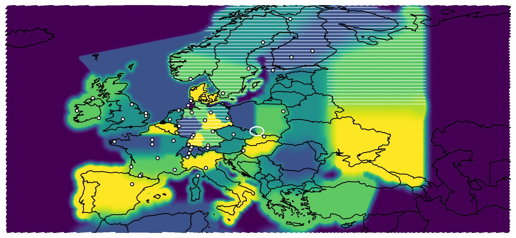
Figure 1 Overview of the model domain indicating flux categories (colored areas) and observation sites (white dots), modified from Part 1 (Bruch et al., 2025a). Each connected area of equal color defines one flux category for anthropogenic emissions, except in Germany and the Netherlands, where the categories are split up further to distinguish agriculture emissions from other sectors. In white hatched regions, natural fluxes form additional flux categories because large natural fluxes are expected. Close to the eastern and western domain boundary (dark blue), emissions are not adjusted by the inversion. Fugitive emissions from the Upper Silesian Coal Basin (white ellipse) define their own flux category.

2.2 A priori fluxes

For the a priori fluxes outside Germany, we combine CAMS-REG (Kuenen et al., 2021, 2022) for anthropogenic emissions with wetland emissions from the CAMS global inversion-optimized dataset (Segers and Houweling, 2020), version v22r2. For Germany, we use emissions obtained from the inventory agencies, that is, the Umweltbundesamt (German Environmental Agency, Stefan Feigenspan, Theo Wernicke, and Christian Mielke, personal communication, 2024) and the Thünen Institute (Roland Fuß and John Akubia, personal communication, 2024). Moreover, we consider emissions from rivers and streams (Rocher-Ros et al., 2023), as well as oceans (Weber et al., 2019).

2.3 Transport simulation

To connect surface fluxes and observations, we need to simulate atmospheric transport. This simulation is done using the numerical weather prediction model ICON (Zängl et al., 2015) with the module for Aerosol and Reactive Trace gases (ART) (Rieger et al., 2015; Schröter et al., 2018) at a horizontal resolution of 6.5 km. Initial and lateral boundary conditions for the CH₄ concentrations are taken from the CAMS global inversion-optimized dataset (Segers and Houweling, 2020), version v22r2. To mitigate a possible bias in the lateral boundary conditions, we construct a smooth correction field that is added to all model predictions of the boundary contributions. This far-field correction is constructed based on observations for which the model predicts clean air with small influence of emissions from within our domain. We estimate transport uncertainties and their correlations using an ensemble of 12 members with slightly different meteorology, derived from the operational numerical weather prediction at DWD (Schraff et al., 2016).

2.4 Observations

We use CH₄ concentration observations from the European Obspack (ICOS RI et al., 2024) as provided on the Integrated Carbon Observation System (ICOS) carbon portal. The hourly observations are filtered by time of day and wind speed to use only observations that can be predicted well by the transport model. We use night time observations (23:00 to 05:00 local mean time) for high mountain stations and afternoon hours (11:00 to 17:00 local mean time) for all other sites, discarding observations at wind speeds below 2 m s⁻¹.

2.5 Bayesian Inversion

To estimate the scaling factors of the flux categories, we use a Bayesian inversion. Denoting the scaling factors as a vector s∈ℝ⁴⁶, the inversion is formulated as the optimization problem

$$\begin{array}{}\text{(1)}& \begin{array}{rl}{\mathit{s}}^{\text{post}}& =\underset{\mathit{s}}{\arg \min }\left\{{\displaystyle \frac{\mathrm{1}}{\mathrm{2}}}[\mathit{y}-{\mathit{H}}^{\prime }(\mathit{s}\left){]}^{\top }{\mathbf{R}}^{-\mathrm{1}}\right[\mathit{y}-{\mathit{H}}^{\prime }\left(\mathit{s}\right)]\right.\\ & \left.+{\displaystyle \frac{\mathrm{1}}{\mathrm{2}}}(\mathit{s}-{\mathit{s}}^{\text{prior}}{)}^{\top }{\mathbf{B}}^{-\mathrm{1}}(\mathit{s}-{\mathit{s}}^{\text{prior}})\right\}.\end{array}\end{array}$$

Here, y denotes a vector of all observations and H^′(s) is the model prediction for these observations, which includes the previously mentioned far-field correction. R is the error covariance matrix of the model–observation mismatch and B is the error covariance matrix of the a priori scaling factors s^prior. Since s describes prefactors to the a priori emissions, we initially set ${\mathit{s}}_k^{\text{prior}}=\mathrm{1}$ for all k. In B we assume an a priori uncertainty of 2σ=0.8 (two standard deviations) for the scaling factors of most regions. This gives the inversion enough freedom to adjust the scaling factors. In large distance from Germany, the a priori uncertainty is reduced to 2σ=0.5 (see Fig. 2b), and for emission sectors in Germany and the Netherlands we use 2σ=1.0.

The construction of R based on the transport ensemble is discussed in detail in Part 1 (Bruch et al., 2025a). In Eq. (1), R can be estimated using either a priori or a posteriori fluxes. This defines two slightly different methods that are introduced in Sect. 2.5 of Part 1 as “prior R” and “posterior R” inversion. Here, we only consider the average of the two results and the union of the two posterior uncertainty ranges.

2.6 Posterior uncertainties

To estimate the uncertainties of posterior fluxes conservatively, we repeat the inversion 50×2 times with each of the 50 observation sites excluded once for each of the two approximations for R. The lower and upper bounds of the resulting hundred 2σ uncertainty ranges form our posterior 95 % confidence interval. This ensures that a result that is only based on a single observation site will not be considered significant.

2.7 Inversion time window

The scaling factors are estimated separately for each month in 2021 by using only observations from the selected month. The results for different months are thus independent. But since the posterior uncertainty estimates include systematic uncertainties, we assume that uncertainties from different months are correlated.

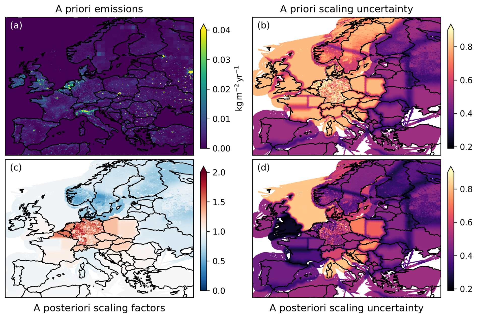
Figure 2 Full-year averages of (a) a priori fluxes, (b) a priori uncertainty on scaling factors, (c) a posteriori scaling factors, and (d) a posteriori uncertainty on scaling factors. Multiplying the a priori emissions (a) with the scaling factors (c) yields the a posteriori emissions. (b) and (d) show half of the 95 % confidence interval of the fluxes relative to the a priori fluxes, i.e., a 2σ uncertainty of 0.5 on the a priori appears as 0.5 on the color scale. The direct comparison indicates the uncertainty reduction. The smooth boundaries between two regions with separate scaling factors appear as darker lines because these scaling factors are assumed to be initially uncorrelated.

3 Results

3.1 Resulting scaling factors

Figure 2 presents an overview of (a) the a priori CH₄ fluxes accumulated over the year 2021, (c) the resulting scaling factors averaged over 2021, and the respective uncertainties (b, d). The a posteriori scaling factors (Fig. 2c) show the correction to the a priori emissions obtained in the inversion. A considerable increase in emissions is found for Germany and the Benelux. Lower emissions compared to the a priori are predicted for Scandinavia (see discussion in Sect. 4.3). The scaling factors should be considered jointly with their uncertainties. The comparison of Fig. 2b and d shows a substantial uncertainty reduction for Germany and most of the surrounding countries, for which we chose a high a priori uncertainty.

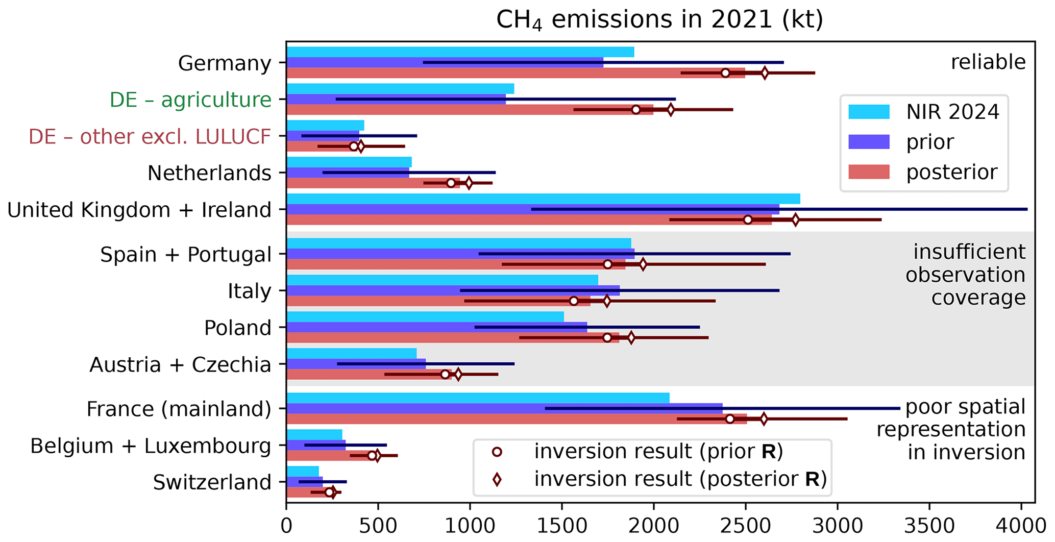
Figure 3 National CH₄ emission estimates comparing reported (NIR), prior, and posterior fluxes for 2021 with horizontal lines indicating 95 % confidence intervals. Countries are grouped by the expected robustness of their inversion results. Some neighboring countries are combined to obtain more accurate results. For Germany, the inversions can resolve the agricultural sector, though the separation against natural and LULUCF fluxes is difficult. All other anthropogenic sectors are combined in the category “other excl. LULUCF”. The inclusion of two inversion methods (“prior R” and “posterior R”, markers) provides an estimate of the methodological uncertainty. Accumulated emissions from national inventory reports (NIR) to the UNFCCC submitted 2024 (including LULUCF emissions) are shown for reference (light blue bars, UNFCCC, 2024). For France (Citepa, 2024) and the United Kingdom (Department for Energy Security and Net Zero, 2024), the light blue bars show emission data from the respective inventory agencies excluding overseas territories and crown dependencies. Posterior uncertainties that are asymmetric with respect to flux estimates such as in Switzerland indicate the strong influence of a single observation site.

For a more detailed comparison of a priori and a posteriori emissions and uncertainties, we consider selected national emission estimates in Fig. 3. Reliable inversion results are expected for countries or regions with sufficient observation coverage, strong emission signals, representation in the respective flux categories, and only moderate issues due to complex topography. These criteria are met for Germany, the Netherlands and the United Kingdom plus Ireland as grouped in Fig. 3. For Germany (first entry in Fig. 3), the total posterior CH₄ emissions (red bar) are (32±19) % higher than the anthropogenic emissions including LULUCF reported to the UNFCCC in 2024 (light blue bar). The direct comparison to the reporting neglects the unreported natural fluxes, but for Germany these are expected to be small because all relevant soil emissions are included in the LULUCF sector. The inversion significantly increases emission estimates from the agriculture sector while the combined other sectors remain nearly unchanged. Note, however, that the uncertainty in the sector attribution is large (horizontal lines, see further discussion in Sects. 3.4.2 and 4.3).

For the Netherlands, we also find significantly higher emissions than in the inventory. Compared to Germany, the attribution to sectors has an even larger uncertainty, associated with fewer observations that could distinguish the sectors. Nevertheless, the total emissions from the Netherlands are comparably well constrained by the observations. For the United Kingdom and Ireland – which we combine to obtain more accurate results – the inversion yields a strong uncertainty reduction while hardly changing the total emissions, indicating a good agreement of observations and national inventory.

In most countries, the observations do not cover the whole country, or the inversion results rely on few observations. In Fig. 3 (gray-shaded part) we provide emission estimates also for countries or regions affected by this issue, though these have a large posterior uncertainty. Another issue arises from the definition of the flux categories, which do not necessarily follow country borders (see Fig. 1). In France, Belgium, and Switzerland, the inversion scales flux categories that overlap multiple countries¹. This implies that national emission estimates derived for these countries have an additional uncertainty and artificial correlations with neighboring countries. However, this is of no concern for our application for Germany. The national emission estimates are computed from the gridded posterior fluxes and precisely follow the country borders as shown in Fig. 2. The scaling factors and uncertainties of all flux categories are listed in Fig. A1 for completeness.

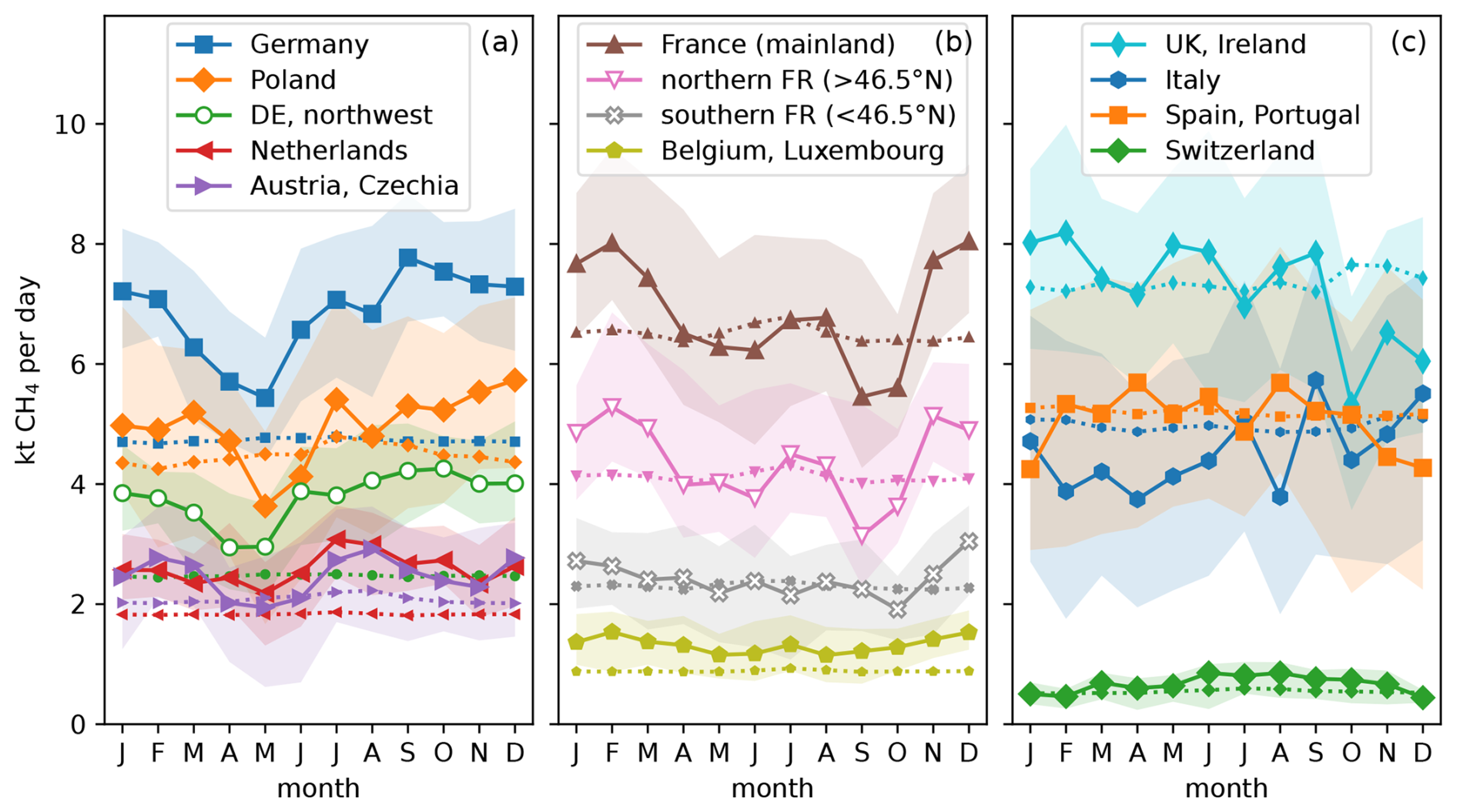
Figure 4 Monthly posterior emission rates for selected countries or regions. Colored areas show the posterior uncertainties, and dotted lines with small markers indicate prior emission rates. In the prior, only the natural and LULUCF fluxes are time-dependent. The panels show (a) countries with minimum in May, (b) countries with a maximum in winter, and (c) other countries and regions. For France and Germany, selected regions are shown additionally (white markers). “DE, northwest” includes Rhineland-Palatinate, Saarland, Hesse, North Rhine-Westphalia, Lower Saxony, Schleswig-Holstein, Bremen and Hamburg.

3.2 Seasonal cycle

Although the national emission estimates are given for the full year, a closer examination of the seasonal cycle provides additional insights. Figure 4 shows the monthly emission rates for the countries considered in Fig. 3. While the seasonal cycle is strikingly different depending on the region, we find some recurrent features. For Germany, Poland, the Netherlands, and Austria plus Czechia (panel a in Fig. 4), the posterior emission rates have their minimum in May. A local minimum between April and June is also found for northern France and Belgium plus Luxembourg, see panel (b). In most countries, this minimum is followed by a local maximum in July or August, which is most prominent in the Netherlands and Austria plus Czechia (panel a).

The differences between the regions become larger in autumn and winter. In September, posterior emission rates reach their maximum in Germany and Italy, and their minimum in (northern) France. France and Belgium plus Luxembourg have their highest emission rates in winter, when Switzerland and Spain plus Portugal have their minimum. For some regions – most notably Italy and the United Kingdom plus Ireland – no clear pattern is found in the seasonal cycle for 2021 (panel c in Fig. 4).

The seasonal cycle in the inversion results may be partially influenced by the observation coverage because many stations lack data covering the whole year. To avoid this effect, we repeated the inversion using only stations which provide data for at least 20 days of each month. The seasonal cycle in these results does not change significantly, see Fig. A2. We further note that there is a seasonal cycle in the observations (East et al., 2024), which is captured well by the far field in the model though (see Fig. A3). This “far field” is defined as CH₄ transported into our domain from the lateral boundaries. A possible bias in the lateral boundary conditions could influence the seasonal cycle in the estimated fluxes. Moreover, the different meteorology in summer and winter – especially influencing the planetary boundary layer and vertical mixing (Seidel et al., 2012) – can lead to a seasonal bias in our transport model (Bessagnet et al., 2016; Canepa and Builtjes, 2017). This highlights the need for careful interpretation of the seasonal cycle, as meteorological differences could introduce biases that mask true emission patterns. Another potential contribution to the seasonal cycle could arise from neglecting the OH sink of CH₄ in our limited domain (Logan et al., 1981).

3.3 Validation

A straightforward validation of the inversion results is possible using independent validation stations. Having excluded each station once in separate inversion runs, we can use every station as an independent validation site in the respective inversion run. Figure 5 shows histograms of the root mean square error (RMSE) statistics obtained from the model–data mismatch before and after the inversion. The validation stations agree on average significantly better with observations when using a posteriori emissions compared to the a priori. A comparison of the same histograms for the different methods of estimating uncertainties introduced in Part 1 (Bruch et al., 2025a) shows no significant differences (see Fig. A4).

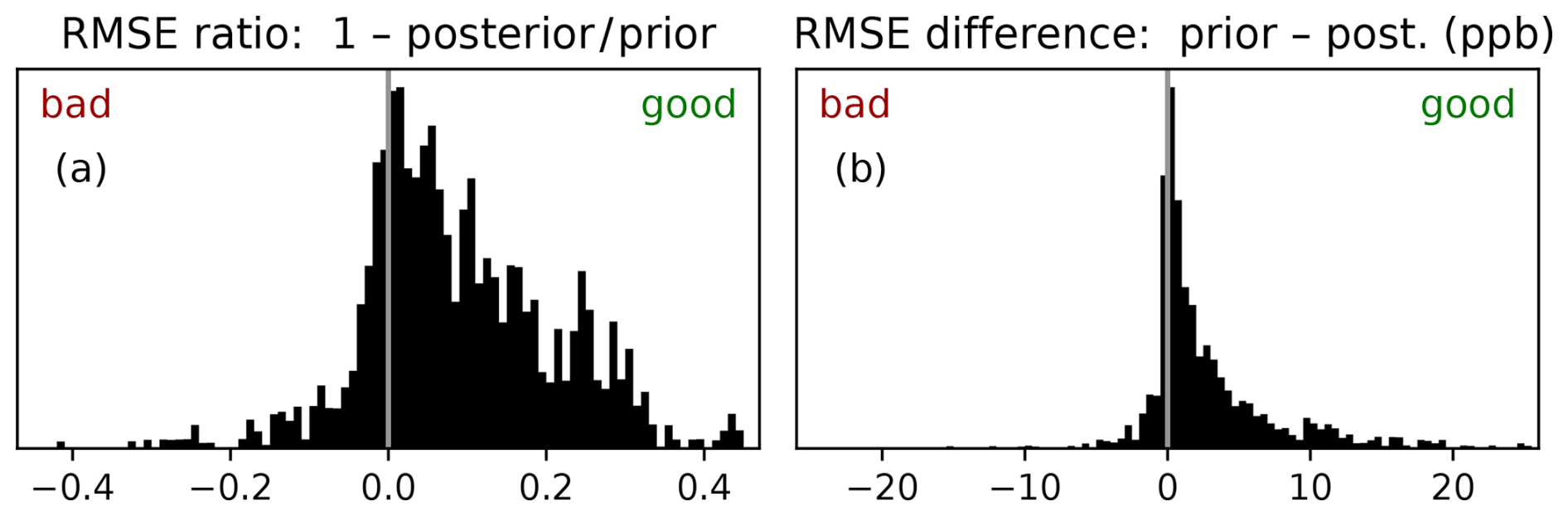
Figure 5 Statistics of the relative (a) and absolute (b) improvement of the model–observation mismatch by the inversion at independent validation stations. Each station and month is considered separately in its own inversion, with the validation station excluded from the inversion to remain independent. The histograms show (a) $\mathrm{1}-r^{\text{post}}/r^{\text{prior}}$ and (b) r^prior−r^post where r^post and r^prior refer to the RMSE of the model–observation comparison in the case of posterior scaling and prior scaling, respectively. Each time series contributing to the histogram is weighted by the number of its data points. We consider all data points within the daily time window without filtering for wind speed or model–observation mismatch and without the far-field correction introduced in Part 1 (Bruch et al., 2025a) to keep the comparison as close as possible to the original data. Positive values indicate an improvement in the model prediction due to the inversion.

3.4 Potential for detecting emissions

In this section, we complement the uncertainty estimates of our inversion results by separate measures for the sensitivity of the posterior to true emissions. The potential for detecting emissions from different sources can be identified using the posterior error covariance matrix B_post. However, the real error reduction is also influenced by the far-field correction and the filtering of observations as detailed in Part 1 (Bruch et al., 2025a). These aspects are not fully captured in B_post. We therefore use experiments with a “synthetic”, i.e., defined truth and pseudo-observations to test the full inversion system.

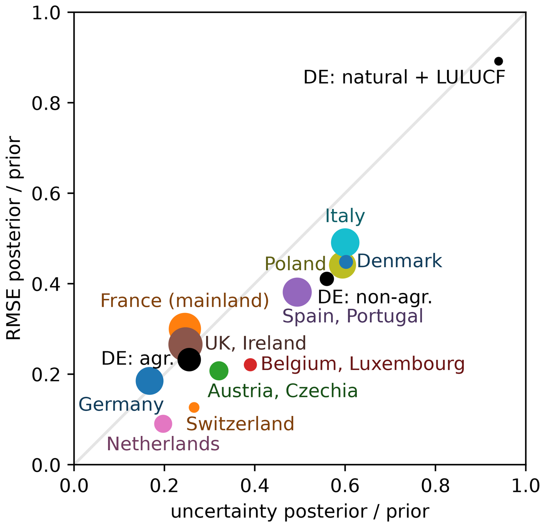
Figure 6 RMSE and mean uncertainty of CH₄ emission estimates in synthetic experiments for selected countries, regions, and German emission sectors. Each of the 100 synthetic experiments uses random true emissions. The vertical axis shows the root mean square (RMS) deviation of the posterior from these true emissions, relative to the RMS deviation of the prior from the truth. Lower values indicate that the inversion improves the emission estimate. The horizontal axis shows the posterior uncertainty relative to the prior uncertainty. Therefore, the bottom left indicates best performance. The disk size indicates the magnitude of the prior emissions.

3.4.1 National emission estimates

We first aim to verify that the inversion yields meaningful posterior emission estimates and uncertainties given a perfect transport model. To this end, we generate 100 random vectors of scaling factors following the probability distribution assumed in the a priori uncertainty. Each vector of scaling factors defines a synthetic truth, and the model prediction for the observations obtained using these scaling factors defines our pseudo-observations. We further add uncorrelated Gaussian noise of standard deviation 2 ppb to these pseudo-observations. Since the pseudo-observations are inferred from the model data, there is no transport error in these synthetic experiments. This construction of pseudo-observations clearly underestimates the true error in the model–observation comparison, but it allows us to test the interplay of far-field correction and inversion in a controlled setup. Synthetic experiments with a simulated transport uncertainty are discussed in Part 1 (Bruch et al., 2025a).

The quality of the model prediction is shown in Fig. 6 for selected countries and German sectors. By comparing to the synthetic truth, we find the prior and posterior error. Their ratio (vertical axis in Fig. 6) shows a significant improvement by the inversion for all considered regions and German sectors, with the exception of German natural and LULUCF fluxes. The uncertainty reduction of the inversion (horizontal axis) provides a realistic estimate of the real error reduction (vertical axis) for the case of high quality observations, ideal transport modeling, and perfect lateral boundary conditions. In some cases (Netherlands, Switzerland, Belgium, and Luxembourg), the real error reduction is significantly better than the uncertainty reduction suggests. This is no surprise because in this synthetic setup the transport error as the main source of uncertainty is switched off. Overall, the synthetic experiments confirm the potential for a strong uncertainty reduction in Central Europe.

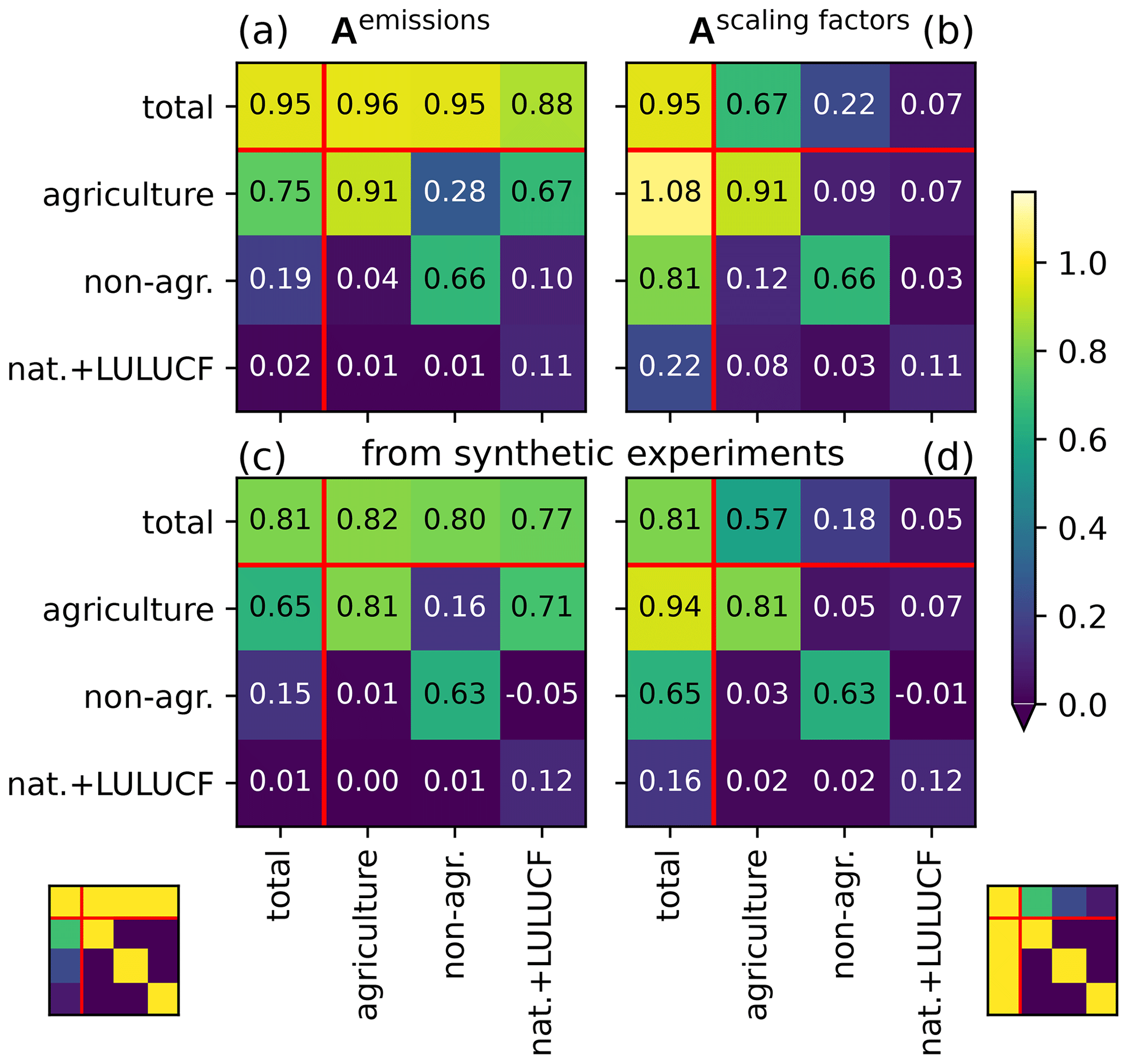
Figure 7 Averaging kernel matrices of German sector emissions (a, c) and scaling factors (b, d). The kernel is estimated using either the posterior covariance matrix (a, b) or 100 synthetic experiments with random truth (c, d). The small matrices on the bottom indicate what we aim for (posterior equals truth). The value 0.96 in the first row (“total”), second column (“agriculture”) of panel (a) means that if in reality all German agriculture emissions were 1 kt higher than in our prior, then we would expect an increase in the posterior total German emissions by 0.96 kt. Similarly, the value 0.67 in the same cell of panel (b) means that increasing real agriculture emissions by 10 % should increase our posterior total emissions by 6.7 %. All matrices are averaged over the whole year. Red lines separate the individual sectors from their sum (“total”). By “non-agr.” we denote anthropogenic emissions excluding agriculture and LULUCF.

3.4.2 Distinguishing sectors in Germany

Within Germany, we distinguish agriculture from other emissions. The discrimination of emission sectors works in the same way as we distinguish emissions from different areas. Each sector has a specific spatial distribution of emissions, which we assume to be correct in the a priori. The predicted CH₄ concentration at the observation sites will therefore depend on how the individual sectors are scaled. In the inversion, the sector emissions are scaled to find optimal agreement of model prediction and observations.

The ability to distinguish sectors can be described by averaging kernel matrices which estimate the dependence of the posterior on the true emissions, ${\mathbf{A}}_{ij}^{\text{emis}}=\partial {\mathit{e}}_i^{\text{post}}/\partial {\mathit{e}}_j^{\text{truth}}$ where e_i denotes emissions from sector i. Since the true emissions e^truth are generally unknown, the averaging kernels A^emis can only be estimated. Figure 7 shows such estimates for A^emis (panels a, c) and the averaging kernel for scaling factors, ${\mathbf{A}}_{ij}^{\text{scaling factors}}=\partial {\mathit{s}}_i^{\text{post}}/\partial {\mathit{s}}_j^{\text{truth}}$ (panels b, d). Assuming a perfect transport model and perfect far field, the averaging kernel matrix can be estimated by ${\mathbf{A}}^{\text{emis}}\approx \mathbf{I}-{\mathbf{B}}_{\text{post. emis}}{\mathbf{B}}_{\text{prior emis}}^{-\mathrm{1}}$ (Rodgers, 2000) using the prior and posterior covariance matrices of the emissions from the “prior R” inversion (see Appendix B1). I denotes the identity matrix. Figure 7a shows this averaging kernel estimate for German sector emissions, extended by a row and column for the total German emissions.

The first row of Fig. 7a indicates that the total German posterior emissions follow changes in every sector with high accuracy (88 % to 96 %). The diagonal of Fig. 7a signifies that changes in the agriculture will be detected very well and also the attribution to the sum of all other anthropogenic sectors excluding LULUCF (“non-agr.”) will be mostly correct. However, LULUCF plus natural fluxes will in large parts be falsely attributed to the agriculture (second row, last column). Note that ideally, the first row and the diagonal elements would be close to 100 % (color-coded in the small matrix bottom left). The averaging kernel A^{scaling factors} in Fig. 7b shows that the influence of LULUCF and natural emissions on the posterior scaling factor for agriculture emissions remains low (second row, last column). But if all emissions are scaled by the same factor (first column), the changes will be mostly attributed to the agriculture sector. This effect is expected because the agriculture sector has the highest absolute a priori uncertainty, which makes changes in agriculture more likely than changes in any other sector. A formal derivation of this argument is presented in Appendix C.

The averaging kernel matrices in Fig. 7a and b are estimated based on the “prior R” inversion while neglecting the far-field correction. We complement these by a statistical estimate of the averaging kernels using 100 synthetic experiments with random truth (see Appendix B2), shown in Fig. 7c and d. Here, the far-field correction is applied as implemented in our processing chain. While these statistical estimates reproduce all qualitative features in the averaging kernels, the matrix entries estimated using synthetic experiments are generally lower. This is likely due to the far-field correction and indicates that deviations from the prior emissions may be underestimated by our inversion. Importantly, both presented strategies for estimating the averaging kernels assume a perfect transport model. The real sensitivity of the posterior to the true emissions is therefore expected to be lower.

4 Discussion

Our inversion system combines precise in situ observations, accurate a priori fluxes from national reporting, the ICON–ART transport model at 6.5 km resolution, and an ensemble-estimated transport uncertainty. We further rely on CAMS boundary conditions and high-resolution meteorological fields from operational numerical weather prediction. This yields in general a good agreement between the model prediction and filtered observations, allowing us robust emission estimates for well-observed countries, such as Germany. We compare top-down CH₄ emission estimates to the reported German inventory and its agriculture sector with enough accuracy to lay the technical foundations for a future long-term observation-based national inventory verification. This section discusses our main results (Sect. 4.1), including a comparison with other studies (Sect. 4.2). We elaborate the limitations of our approach (Sect. 4.3) and its potential for the development of observation-based national inventory verification to inform climate policy (Sect. 4.4).

4.1 Key findings

Firstly, we find that our top-down CH₄ emission estimates are significantly higher than reported for Germany. Secondly, we identify the agriculture sector and possibly LULUCF and natural fluxes as the likely main source of this discrepancy. Thirdly, we recall from Part 1 (Bruch et al., 2025a) that the transport error simulated in the meteorological ensemble leads to an uncertainty of 2 % on the total German CH₄ emissions.

4.2 Comparison to other methods

Our Eulerian approach with sectoral segregation differs from other studies on CH₄ inversions for single countries, e.g., Henne et al. (2016) for Switzerland and Ganesan et al. (2015) for the United Kingdom that use Lagrangian transport models. The latter both qualitatively attribute deviations from the inventory reporting to the agriculture sector by comparing the spatial and/or temporal patterns in the posterior fluxes to sectoral a priori fluxes. A similar strategy for sectoral segregation based on a known spatial distribution of fluxes is followed by Varon et al. (2022) and analyzed by Cusworth et al. (2021). For deriving sector estimates, some inversions assume a spatial correlation of gridded emissions within each sector (Rödenbeck et al., 2003; Meirink et al., 2008b; Bergamaschi et al., 2010). Based on the same assumption, Steiner et al. (2024b) and Tenkanen et al. (2025) construct ensembles of perturbed a priori fluxes to distinguish natural and anthropogenic fluxes utilizing the CarbonTracker Data Assimilation Shell (van der Laan-Luijkx et al., 2017). Notably, Tenkanen et al. (2025) avoid the lateral boundary problem by simulating transport globally with nested zoom in Europe to estimate Finnish CH₄ emissions on a coarse resolution of 1° × 1°. In the present work, we take the next step by validating sectoral emissions reported to UNFCCC and analyzing possible false attributions, making use of a significantly higher model resolution.

Our results are qualitatively in line with the discrepancy of top-down estimates and UNFCCC reporting for Germany and the Benelux found in different regional inversions for the years 2018 and earlier (Petrescu et al., 2023; Bergamaschi et al., 2022, 2018; Steiner et al., 2024b). Furthermore, it appears as a robust feature in our results that emissions from the UK plus Ireland agree well with reported emissions, in line with Bergamaschi et al. (2022) for the year 2018. For the French emissions, our inversion shows a tendency towards slightly higher emissions similar to Steiner et al. (2024b), whereas other inversions suggest significantly higher emissions (Petrescu et al., 2023; Bergamaschi et al., 2022).

4.3 Limitations

Although we simulate emissions and transport in a large domain, we can only provide reliable emission estimates for selected countries (compare Fig. 3). Regions without notable uncertainty reduction and regions with known modeling difficulties do not benefit from our model setup. In Scandinavia, we find strong wetland emissions with insufficiently modeled fine-scale spatial and temporal variability. Combined with only small signals from non-LULUCF anthropogenic emissions, this leads to a low signal-to-noise ratio, which prevents conclusive results for Scandinavia. Furthermore, the synthesis inversion may be prone to underestimating large localized sources due to transport errors – an issue we address in Part 1 (Bruch et al., 2025a).

Another limitation comes from the challenges for the regional flux inversion caused by biases in the lateral boundary conditions. The uncertainty in lateral boundary concentrations motivates the far-field correction that is discussed in Part 1 (Bruch et al., 2025a). We expect that the far-field correction leads to more robust estimates for well-observed emissions, but it may also cause a bias towards the prior and towards lower emission estimates.

In our highly resolved transport simulation, every flux category is numerically expensive. Aiming to validate reported German emissions, we could reduce the state space of the inversion to only 46 scaling factors with monthly time resolution. This substantially limits the spatial and temporal variations that can be represented in the inversion. This approach is justified if the a priori fluxes already provide a realistic spatial distribution of all major CH₄ sources within each flux category. While this may be the case in Germany and neighboring countries, the constant scaling factors for large flux categories in more distant regions may be oversimplified and could lead to less accurate results in these regions. Moreover, adjusting only a few degrees of freedom may not be sufficient to obtain realistic flux estimates in regions with limited or highly uncertain information on a priori fluxes, such as Scandinavia.

When constructing the state space, we unevenly distributed the 46 degrees of freedom on our model domain – using 11 degrees of freedom for Germany and only four for mainland France plus Belgium and Luxembourg. But the choice of flux categories affects the results and can lead to biases depending on the location of the observations (Kaminski et al., 2001). In our application, this effect is small because of the good observation coverage in Germany. This is checked in Part 1 (Bruch et al., 2025a) using sensitivity tests.

We exploit the sectoral discrimination of emission in a well-observed region as a key feature of our inversion method. This relies heavily on an accurate spatial distribution and completeness of the a priori fluxes, which appears to be sufficient for the major emitting sectors in Germany. Furthermore, the sector discrimination relies on resolving comparably small spatial scales, which poses a challenge to the transport modeling. A general problem in sector attribution is that sectors with large absolute uncertainty – such as agriculture – may be falsely blamed for any change in total emissions when the observations do not clearly distinguish the sectors (see Appendix C). By quantifying this effect in the averaging kernels (see Fig. 7), we confirmed that in Germany agriculture can be distinguished from other anthropogenic emissions excluding LULUCF. Small sectors like natural plus LULUCF fluxes could not be reliably distinguished from large sectors such as agriculture, and we therefore combined smaller sectors like waste and public power into the larger category “non-agr.”.

4.4 Implications for future research

We chose the synthesis inversion for the first application of our modular inversion system, but designed this framework to be expandable to other inversion methods. For instance, most of the steps in the inversion can be applied with only minor adjustments when replacing the flux categories by an ensemble of randomly perturbed surface fluxes, similar to Steiner et al. (2024b), or by grid cell clusters as used by Estrada et al. (2025). Such applications with a larger state space are limited by the computational effort of the transport simulation, which is much higher than the computational effort of the inversion itself. Similar to the inversion method, the far-field correction can be replaced by a different strategy for mitigating a boundary bias. For example, one could construct the far field based on an ensemble of boundary concentrations.

Further possibilities of extension involve other observation types, including satellite data. Our Eulerian system allows in principle the handling of large observation datasets without prohibitive computational effort, albeit changes in the construction and handling of R may be required when reaching ≳10⁵ observations per time window. This potential is leveraged by many inversion systems that use Eulerian transport simulations (e.g., Varon et al., 2022; Meirink et al., 2008a; Bergamaschi et al., 2013). The increasing availability of satellite data is especially interesting for constraining concentrations and emissions in regions with few or no ground-based observations, such as near the boundaries of our domain, which is an aspect to be addressed in future studies.

We identified potentials and risks in separating sectors based on the spatially highly resolved distribution of fluxes. Extending this by temporal profiles for a priori fluxes offers a yet untapped potential for future improvement of our system. Moreover, our inversion could benefit from an a priori emission ensemble reflecting the uncertainty in the spatial and temporal distribution of the fluxes. It remains to be explored whether improvements in distinguishing sectors can be achieved in our system using co-tracers such as ethane for fossil CH₄ emissions (Ramsden et al., 2022; Mead et al., 2024) or by distinguishing carbon isotopes (Basu et al., 2022; Thanwerdas et al., 2024; Chandra et al., 2024).

5 Conclusions

We presented first results from a novel system for regional flux inversion designed to validate national CH₄ emission reporting. Applying this method to Central Europe in 2021 with a focus on Germany, we found significantly higher emissions from Germany and the Benelux compared to the reporting. Careful estimation of posterior uncertainties revealed for the investigated year that the total German posterior emissions are (32±19) % higher than the respective anthropogenic emissions reported to the UNFCCC (submission 2024). With our inversion method the difference is attributed to emissions from the agriculture sector, possibly with contributions from the LULUCF sector and natural sources. Our results were confirmed by validation with independent observation sites and by an exhaustive range of sensitivity tests presented in Part 1 (Bruch et al., 2025a). Synthetic experiments with known truth revealed the method's ability to distinguish the agricultural from the non-agricultural sectors in Germany, whereas disentangling possible influences from natural and LULUCF sources requires further work and possibly more observations.

A methodological comparison to other regional inversion systems highlights the advantages of our method for the purpose of distinguishing emission sectors and its suitability for validating national emission estimates. The qualitative gap between UNFCCC reporting and our estimates for Germany and the Benelux is consistent with earlier works (Petrescu et al., 2023; Bergamaschi et al., 2022, 2018; Steiner et al., 2024b). We complement these studies by providing an emission estimate for the German agriculture sector that can be directly compared to the national reporting, revealing a significant mismatch.

In this study we presented the first application of an extensible, novel inversion system. Future developments may include the integration of satellite data, the incorporation of temporal profiles, a more comprehensive treatment of boundary conditions and flux uncertainties using ensemble methods, and an extension of the state space. The close connections to operational numerical weather prediction – especially in the underlying transport simulation – and the modular design establish the potential for long-term operational support of national emissions reporting.

Appendix A: Supplementary figures

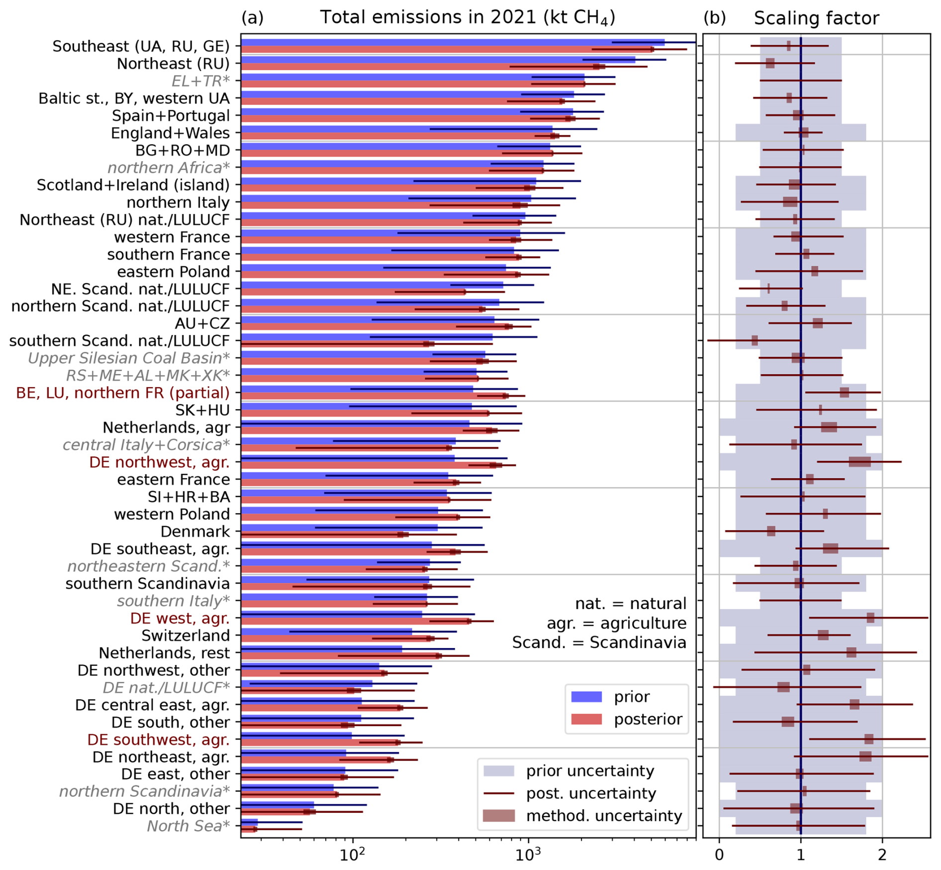
Figure A1 Prior and posterior emissions (a) and scaling factors (b) for all flux categories, ordered by prior emissions. Horizontal lines indicate 95 % confidence intervals. See Fig. 1 for the geographical definition of the flux categories and Fig. 2 for the resulting map of scaling factors. (a) If no sector is explicitly specified, the flux categories contain all anthropogenic fluxes excluding LULUCF. For flux categories marked with an asterisk, the inversion does not reduce the absolute uncertainty. Thus, reliable information is only gained by our inversion for flux categories without asterisk (see Sect. 2.6). Red color of the category names indicates a statistically significant increase of emissions. (b) Scaling factors are the raw results of our inversion, though here they are already combined for the whole year. The posterior scaling factor is defined as the center of the methodological uncertainty range indicated by brown boxes.

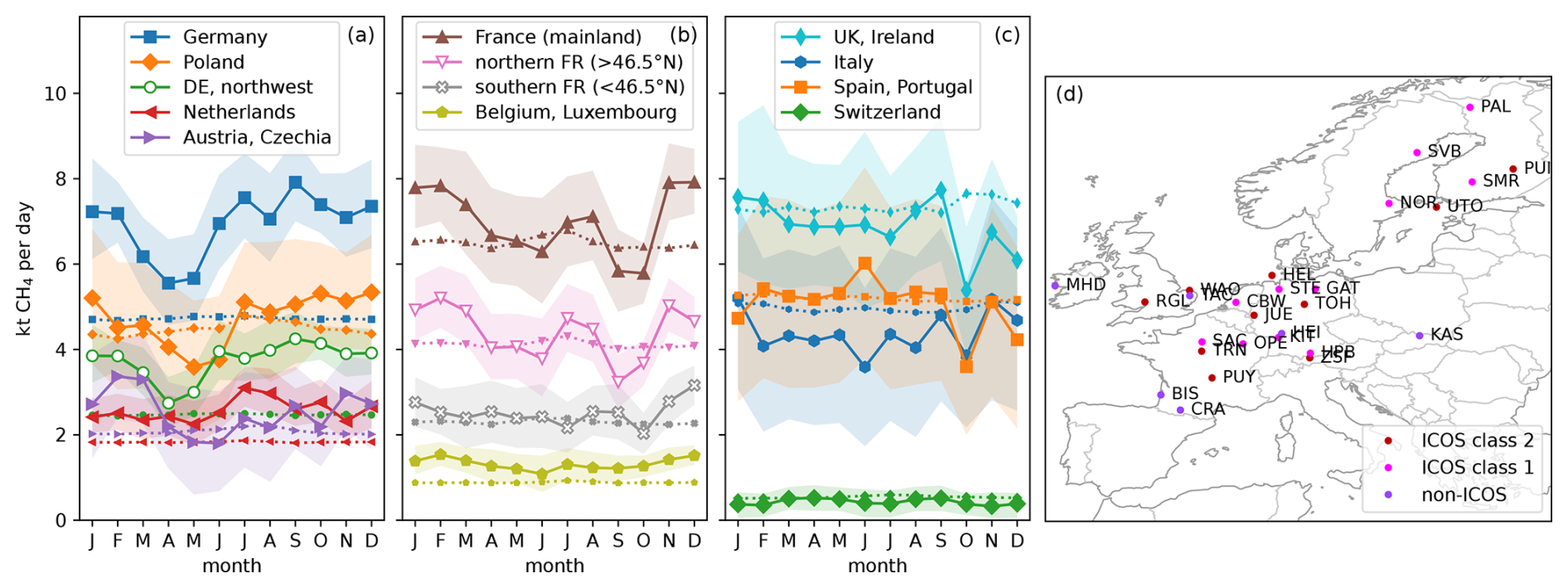
Figure A2 (a–c) Seasonal cycle when using only observations from stations that were active during the whole year. We select those stations and sampling heights, for which we used at least two data points per day on at least 20 days of each month in 2021 in our main inversion. This selects 27 stations shown in (d) with 8.3×10⁴ data points for the inversion, compared to 50 stations with 1.29×10⁵ data points in the reference case (compare Fig. 4). Colored areas show the posterior uncertainties (95 % confidence intervals), which were computed without excluding individual stations from the inversion and are therefore smaller than in Fig. 4. Prior emission rates are shown as dotted lines with small markers.

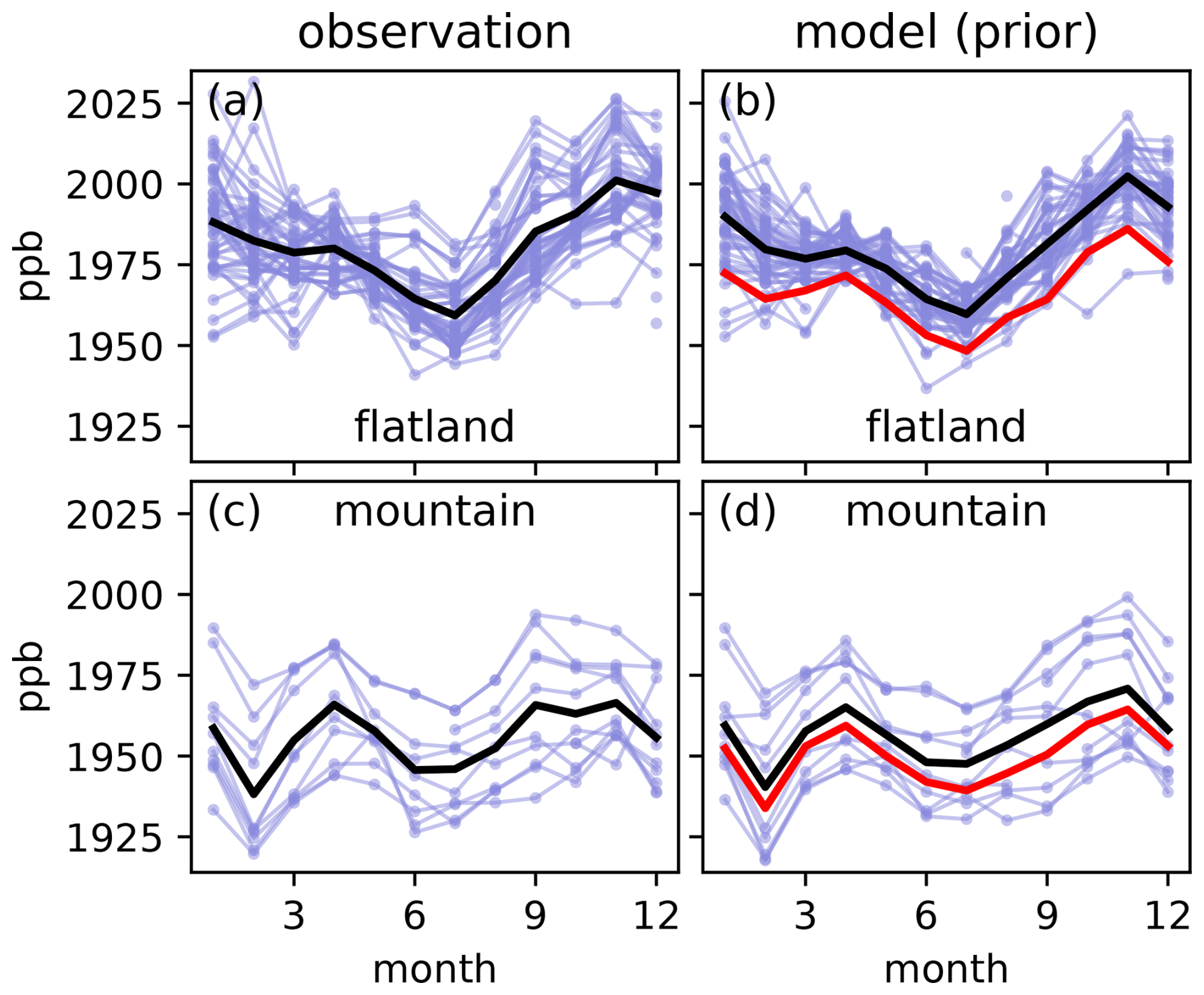
Figure A3 Seasonal cycle in observations at stations with elevation below 500 m above sea level (a, b) and above 1000 m (c, d), supplementary to the discussion in Sect. 3.2. Thin blue lines represent the 10 % quantile of each month, station, and sampling height for (a, c) observations and (b, d) model predictions (prior). The 10 % quantile is chosen to minimize the effect of local pollution. Thick black lines indicate the mean of all selected stations and sampling heights. Thick red lines in (b) and (d) show the 10 % quantile of the modeled far-field concentration. The flatland stations show a pronounced seasonal cycle with minimum in summer for both model and observations. This cycle is dominated by the contribution of the far field. The mountain stations have a weaker seasonal cycle.

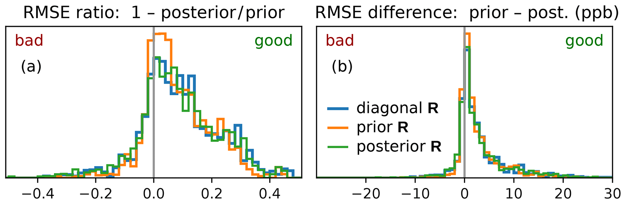
Figure A4 Statistics of the relative (a) and absolute (b) improvement of the model–observation mismatch at independent validation stations for different choices of the error covariance matrix R discussed in Part 1 (Bruch et al., 2025a). The figure is analogous to Fig. 5, where the visualization and the data selection is explained. Here, we distinguish three inversion methods that differ in how R is constructed, as introduced in Sect. 2.5 of Part 1. No clear advantage of one method over the others can be seen. The diagonal R inversion has the lowest posterior RMSE at validation sites, followed by the posterior R and prior R inversion, but the differences are not statistically significant.

Appendix B: Averaging kernel matrices

As introduced in Sect. 3.4.2, the averaging kernel matrices A^emis and A^{scaling factors} estimate the change in the posterior when changing the truth, ${\mathbf{A}}^{\text{emis}}=\partial {\mathit{e}}^{\text{post}}/\partial {\mathit{e}}^{\text{truth}}$ where e denotes the vector of emissions. Here, we summarize how these matrices are estimated using either the error covariance matrices B and B_post or the statistics from inversion runs with synthetic truth.

B1 Analytic estimate using error covariance matrices

We first estimate the sensitivity of the posterior scaling factor to the true emissions under the assumption that the transport model, far field, observations, and the a priori spatial distribution within each flux category are perfect. Under these idealized assumptions, the model–observation mismatch for given scaling factors s is $\mathit{\mu }\left(\mathit{s}\right)=\mathit{y}-\mathbf{H}\mathit{s}-{\mathit{x}}^{\text{ff}}=\mathbf{H}({\mathit{s}}^{\text{truth}}-\mathit{s})$ where s^truth denotes the true scaling factors and we parametrize the model prediction by ${\mathit{H}}^{\prime }\left(\mathit{s}\right)=\mathbf{H}\mathit{s}+{\mathit{x}}^{\text{ff}}$. Our “prior R” inversion will now maximize

$$\begin{array}{ll}{\displaystyle }P\left(\mathit{s}\right)& {\displaystyle }\propto \exp \left[-{\displaystyle \frac{\mathrm{1}}{\mathrm{2}}}(\mathit{s}-{\mathit{s}}^{\text{truth}}{)}^{\top }{\mathbf{H}}^{\top }{\mathbf{R}}^{-\mathrm{1}}\mathbf{H}(\mathit{s}-{\mathit{s}}^{\text{truth}})\right.\\ \text{(B1)}& {\displaystyle }& {\displaystyle }\left.-{\displaystyle \frac{\mathrm{1}}{\mathrm{2}}}(\mathit{s}-{\mathit{s}}^{\text{prior}}{)}^{\top }{\mathbf{B}}^{-\mathrm{1}}(\mathit{s}-{\mathit{s}}^{\text{prior}})\right]\text{(B2)}& {\displaystyle }& {\displaystyle }\propto \exp \left[-{\displaystyle \frac{\mathrm{1}}{\mathrm{2}}}(\mathit{s}-{\mathit{s}}^{\text{post}}{)}^{\top }{\mathbf{B}}_{\text{post}}^{-\mathrm{1}}(\mathit{s}-{\mathit{s}}^{\text{post}})\right].\end{array}$$

This yields ${\mathit{s}}^{\text{post}}={\mathit{s}}^{\text{prior}}+\mathbf{A}({\mathit{s}}^{\text{truth}}-{\mathit{s}}^{\text{prior}})$ with the averaging kernel $\mathbf{A}=\mathbf{I}-{\mathbf{B}}_{\text{post}}{\mathbf{B}}^{-\mathrm{1}}$ and the posterior error covariance matrix ${\mathbf{B}}_{\text{post}}^{-\mathrm{1}}={\mathbf{H}}^{\top }{\mathbf{R}}^{-\mathrm{1}}\mathbf{H}+{\mathbf{B}}^{-\mathrm{1}}$ (Rodgers, 2000). Knowing B and B_post, we can compute the averaging kernel A to estimate how the posterior scaling factors depend on the true scaling factors.

B2 Statistical estimate using synthetic experiments

In the statistical approach, we estimate the sensitivity of posterior scaling factors $\mathit{\xi }:={\mathit{s}}^{\text{post}}-{\mathit{s}}^{\text{prior}}$ to changes in the synthetic truth $\mathit{\zeta }:={\mathit{s}}^{\text{truth}}-{\mathit{s}}^{\text{prior}}$ using 100 synthetic experiments with random synthetic truth s^truth. Given a sample of N realizations {ξⁿ}_n and {ζⁿ}_n, we aim to find the scaling factor averaging kernel matrix A that solves

$$\begin{array}{}\text{(B3)}& \mathbf{A}=\underset{{\mathbf{A}}^{\prime }}{\arg \min }\sum _{n=\mathrm{1}}^N{∥{\mathit{\xi }}^n-{\mathbf{A}}^{\prime }{\mathit{\zeta }}^n∥}^{\mathrm{2}}.\end{array}$$

For $\Vert \mathit{x}{\Vert }^{\mathrm{2}}={\sum }_i{\mathit{x}}_i^{\mathrm{2}}$, differentiation by ${\mathbf{A}}_{ij}^{\prime }$ yields $\mathrm{0}={\sum }_{n=\mathrm{1}}^N{\mathit{\zeta }}_j^n{\left({\mathit{\xi }}^n-\mathbf{A}{\mathit{\zeta }}^n\right)}_i$ for all i,j and thereby

$$\begin{array}{}\text{(B4)}& \mathbf{A}=\mathbf{\Xi }{\mathbf{Z}}^{-\mathrm{1}},{\mathbf{\Xi }}_{ij}=\sum _{n=\mathrm{1}}^N{\mathit{\xi }}_i^n{\mathit{\zeta }}_j^n,{\mathbf{Z}}_{ij}=\sum _{n=\mathrm{1}}^N{\mathit{\zeta }}_i^n{\mathit{\zeta }}_j^n.\end{array}$$

Equation (B4) was used to produce panels (c) and (d) of Fig. 7.

Appendix C: Relevance of absolute prior uncertainty in sector attribution

When observations can detect a change in total emissions but cannot distinguish between different emission sectors, the sector-resolving inversion will change the sectoral distribution based on the prior uncertainties. To understand this problem qualitatively, we consider the worst case: We assume that fluxes from all sectors are uncorrelated in the prior but 100 % spatially correlated such that they cannot be distinguished in the inversion. The a priori probability density for an emission vector e of sector emissions e_i is

$$\begin{array}{}\text{(C1)}& P\left(\mathit{e}\right)\propto \exp \left[-{\displaystyle \frac{\mathrm{1}}{\mathrm{2}}}\sum _i({\mathit{e}}_i-{\mathit{e}}_i^{\text{prior}}{)}^{\mathrm{2}}{\mathit{\sigma }}_i^{-\mathrm{2}}\right],\end{array}$$

where σ_i denotes the a priori standard deviation of e_i. The inversion will estimate the total emissions $e_{\text{tot}}^{\text{post}}$ such that the a posteriori probability density P(e|y) is maximized. But by assumption, these observations do not distinguish between sectors such that the a posteriori probability density fulfills $P\left(\mathit{e}\right|\mathit{y})\propto P(\mathit{e})$ as long as ∑_ie_i is fixed. We thus obtain the posterior emissions of the sectors by maximizing Eq. (C1) with the constraint ${\sum }_i{\mathit{e}}_i=e_{\text{tot}}^{\text{post}}$. By introducing a Lagrange multiplier, one can show² that this implies

$$\begin{array}{}\text{(C2)}& {\mathit{e}}_i-{\mathit{e}}_i^{\text{prior}}=\mathit{\alpha }{\mathit{\sigma }}_i^{\mathrm{2}},\mathit{\alpha }={\displaystyle \frac{e_{\text{tot}}^{\text{post}}-e_{\text{tot}}^{\text{prior}}}{{\sum }_i{\mathit{\sigma }}_i^{\mathrm{2}}}}.\end{array}$$

This shows that sectors with larger absolute a priori uncertainty are disproportionally stronger corrected. Applied to our emission estimates for Germany, this implies that if the observations were unsuitable for distinguishing sectors, the inversion would attribute up to 95 % of the changes in total fluxes to the agriculture sector, which is responsible for 69 % of the total a priori emissions. Fortunately, this worst case scenario is not realistic because the observations do contain information on the different sectors as indicated e.g. by Figs. 6 and 7. But a tendency remains to correct the agriculture stronger than the other sectors.

Appendix D: Attempt to distinguish five sectors in Germany

Our setup for the transport simulation was designed to separate five sectors in Germany: agriculture, natural plus LULUCF, waste, public power, and the sum of all other sectors (“other”). We try to distinguish these sectors in a separate inversion run, in which each of these sectors is scaled separately (sensitivity tests 506 in Part 1 (Bruch et al., 2025a)). This inversion uses 19 separate scaling factors in Germany instead of 11. We find no notable changes in the posterior emissions compared to our reference setup, in which we combined waste, public power, and other into one larger sector “non-agr.” However, the uncertainties and the averaging kernels change considerably. We assume an a priori 2σ uncertainty of ±100 % for each sector-resolving flux category. Thus, splitting the total fluxes in more uncorrelated flux categories reduces the a priori uncertainty of the total fluxes.

Figure D1 shows the averaging kernel matrices (introduced in Sect. 3.4.2 and Appendix B) for the inversion when separating five sectors. These matrices indicate that waste, public power, and “other” cannot be distinguished: The corresponding columns Fig. D1a are approximately equal. Thus, trying to distinguish these sectors does not provide any additional information. By comparing the row and column for “non-agr.” to Fig. 7, we identify drawbacks of the attempt to distinguish smaller sectors. When trying to distinguish five sectors, the false attribution of emissions to the agriculture sectors is more severe than when distinguishing only three sectors (48 % compared to 28 %). Consequently, the expected error reduction in the combined non-agriculture sectors (excluding natural plus LULUCF) is better when considering only three sectors. Qualitatively, this is what we expect from Appendix C for cases where the observations are insufficient to distinguish the considered sectors.

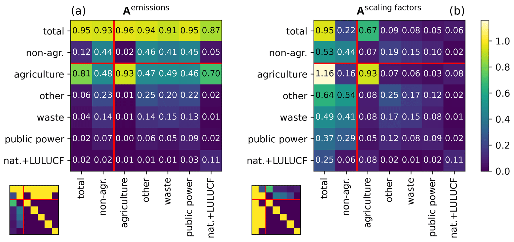
Figure D1 Averaging kernel matrices of German sector emissions (a) and the corresponding scaling factors (b) when trying to distinguish sectors waste, public power and other, estimated using the posterior error covariance matrix. Small matrices at the bottom indicate the ideal result. See Fig. 7 for an explanation of the representation. Panel (a), third row, shows that increasing true emissions in any sector is expected to cause higher posterior agriculture emissions with a false attribution of 46 % to 70 %. The same row in panel (b) shows that when looking at relative changes in the emissions, the influence of the false attribution on the agriculture sector is not very large.