Explaining trends and changing seasonal cycles of surface ozone in North America and Europe over the 2000–2018 period: a global modelling study with NO_x and VOC tagging

Surface ozone, with its long enough lifetime, can travel far from its precursor emissions, affecting human health, vegetation, and ecosystems on an intercontinental scale. Recent decades have seen significant shifts in ozone precursor emissions: reductions in North America and Europe, increases in Asia, and a steady global rise in methane. Observations from North America and Europe show declining ozone trends, a flattened seasonal cycle, a shift in peak ozone from summer to spring, and increasing wintertime levels. To explain these changes, we use TOAST 1.0, a novel ozone tagging technique implemented in the global atmospheric model CAM4-Chem which attributes ozone to its precursor emissions fully by NO_x or $\mathrm{VOC}+\mathrm{CO}+{\mathrm{CH}}_{\mathrm{4}}$ sources and perform multi-decadal model simulations for 2000–2018. Model-simulated maximum daily 8 h ozone (MDA8 O₃) agrees well with rural observations from the TOAR-II database. Our analysis reveals that declining local NO_x contributions to peak-season ozone (PSO) in North America and Europe are offset by rising contributions from natural NO_x (due to increased O₃ production), and foreign anthropogenic- and international shipping NO_x due to increased emissions. Transported ozone dominates during spring. Methane is the largest VOC contributor to PSO, while natural NMVOCs become more important in summer. Contributions from anthropogenic NMVOCs remain smaller than those from anthropogenic NO_x. Despite rising global methane levels, its contribution to PSO in North America and Europe has declined due to reductions in local NO_x emissions. Our results highlight the evolving drivers of surface ozone and emphasize the need for coordinated global strategies that consider both regional emission trends and long-range pollutant transport.

1 Introduction

Ozone near the Earth's surface is primarily formed by the photodissociation of NO₂ molecules by sunlight – the NO₂ molecule breaks down and furnishes atomic oxygen which combines with molecular oxygen in the air to form ozone. The naturally occurring NO₂ concentration in the troposphere is low and cannot alone explain the high ozone observed in the troposphere (Jacobson, 2005; Seinfeld and Pandis, 2016). However, in the modern era especially during the last half of the 20th century, increased industrialization and motorization of society has led to increasing emissions of nitric oxide (NO) (Logan 1983; Beaton et al., 1995; Calvert et al., 1993). NO can interact with peroxy radicals, chiefly produced from naturally and anthropogenically emitted non-methane volatile organic compounds (NMVOCs), carbon monoxide (CO), and methane (CH₄) in the presence of the hydroxyl radical (OH) to form NO₂ which can then produce ozone through the pathway described above (Atkinson 1990, 1994, 1997; Seinfeld and Pandis, 2016). Unsurprisingly, with increasing anthropogenic activities emitting NO, CO, NMVOCs and CH₄, the ozone concentrations in the troposphere and at the surface have risen substantially as compared to the pre-industrial or early-industrial times (Logan, 1985; Crutzen, 1988; Young et al., 2013; UNEP and CCAC, 2021).

Ozone is a highly reactive pollutant that harms human health, vegetation, and the environment due to its oxidative properties. In humans, it causes respiratory inflammation, exacerbates chronic illnesses, and impairs lung function by generating reactive oxygen species that damage cellular structures (Lippmann, 1989; Chen et al., 2007; Devlin et al., 1991; Brook et al., 2004) due to long term exposure as well as short term exposure at high concentrations (Fleming et al., 2018). Ozone disrupts photosynthesis in plants and damages tissues, reducing crop yields and altering ecosystems (Ashmore, 2005; Felzer et al., 2007; Grulke and Heath, 2019; Cheesman et al., 2024); a recent assessment by Mills et al. (2018) shows persistent high levels of ozone adversely affecting various types of crops and vegetation in northern hemispheric regions. Moreover, it contributes to climate change by diminishing the carbon sequestration ability of vegetation and acting as a greenhouse gas (Oeschger and Dütsch, 1989; Sitch et al., 2007; Szopa et al., 2021). In light of these harmful effects, the World Health Organization (WHO) has set safe standards for short-term and long-term human exposure to ozone: on any day, the maximum 8 h average ozone concentration (MDA8 O₃) which must not exceed 100 µg m⁻³ (or ∼51 ppb), and annually, the Peak Season Ozone (PSO), i.e., the maximum value of the six-month running average of MDA8 O₃, must not exceed 60 µg m⁻³ (or ∼30.61 ppb) (WHO 2021).

In order to meet these safe health standards, various national governments - particularly in North America and Europe and more recently in China - have acted to reduce their industrial and vehicular emissions by adopting cleaner fuel and technologies and have successfully managed to bring down their national NO_x and NMVOC emissions substantially (Goldberg et al., 2021; Shaw and Heyst, 2022; Crippa et al., 2023). However, these national efforts of emission reductions have not fully translated into commensurate reductions in local ozone concentrations and health impacts (Seltzer et al., 2020; Parrish et al., 2022). This is due to the long-enough atmospheric lifetime of ozone which allows it to traverse intercontinental distances and affect the air quality of regions far from the location of its chemical production or the location of the emission of its precursors. While the global average tropospheric lifetime of ozone is often cited as approximately 3–4 weeks, a figure largely influenced by more rapid photochemical loss in warmer, humid tropical regions (e.g., Stevenson et al., 2006; Young et al., 2013), the effective lifetime of ozone in air parcels transported within the cooler, drier free troposphere at northern midlatitudes is considerably longer, on the order of several months (e.g., Jacob et al., 1999; Wang and Jacob, 1998; Fiore et al., 2009). This extended lifetime in the primary transport pathway for intercontinental pollution allows ozone to traverse vast distances and enables the northern mid-latitude free troposphere to act as a relatively well-mixed reservoir (Parrish et al., 2020). Moreover, some ozone precursors (e.g., CO and less reactive NMVOCs) also possess atmospheric lifetimes sufficient for intercontinental transport, subsequently contributing to ozone formation in downwind regions far from their original emission sources. Therefore, air quality benefits in regions with declining emissions can be offset by an increasing share of transported ozone from far away regions where emissions are on the rise. Many previous observational-based studies have reported declining peak-ozone trends in North America towards the final decades of the 20th century and the beginning of the 21st century (Wolff et al., 2001; Cooper et al., 2014, 2012, 2020; Chang et al., 2017; Fleming et al., 2018). However, some of these studies and many others – through novel statistical decomposition of observational data – have also pointed out increasing trends in wintertime and background ozone concentrations at many sites in North America, particularly at the US west coast (Jaffe et al., 2003; Cooper et al., 2010; Simon et al., 2015; Parrish and Ennis, 2019; Parrish et al., 2022; Christiansen et al., 2022). Such increases in ozone have also been identified throughout the background troposphere at northern midlatitudes including in the free troposphere, with a peak attained in the first decade of the 2000s (e.g., Parrish et al., 2020; Derwent et al., 2023). Some of these observational studies (e.g., Jaffe et al., 2003) have further correlated the increasing background ozone in western US to increasing emissions in Asia while others (e.g., Cooper et al., 2010) have also employed air mass back trajectory analysis to support their claims. Jaffe et al. (2018) performed a comprehensive knowledge assessment of background ozone in the US and emphasized its growing relative importance and advocated for, among other things, a more strategic observational network and new process-based modelling studies to better quantify background ozone in the US to support informed clean air policies. A number of observational studies have also reported changes in the ozone seasonal cycle in North America, with shifting peaks from summer to springtime (Bloomer et al., 2010; Parrish et al., 2013; Cooper et al., 2014), a reversal of the spring-to-summer shift in peak ozone during mid-twentieth century which was reported in earlier studies (e.g., Logan, 1985) when anthropogenic emissions were increasing in North America. Similarly, for Europe, many studies have observed declining ozone trends since 2000 (Cooper et al., 2014; Chang et al., 2017; Fleming et al., 2018; EEA report, 2020; Sicard, 2021). For Europe too, there have been attempts of statistical decomposition and analyses of observational data in innovative ways to highlight the increasing share of intercontinental transport and the consequent changes in ozone seasonal cycle in recent decades (Carslaw, 2005; Parrish et al., 2013; Derwent and Parrish, 2022).

Reliable, long-term, and publicly accessible monitoring stations across different continents form the backbone of an international consensus on ozone distributions, trends, and health impacts on various populations. These observational networks provide essential data for advanced statistical analyses, which can estimate both transported and locally produced ozone (as seen in many observational studies mentioned earlier). However, such statistical interpretations can be subject to dispute and must be corroborated by well-evaluated atmospheric chemical transport models which simulate atmospheric transport processes explicitly. Together, observational analyses and model-generated results can aid the theoretical development and improvement of simpler conceptual models that capture the essence of the most salient physical and chemical processes that control observed ozone abundances (Derwent et al., 2023).

The hemispheric-scale transport of “foreign” ozone is a phenomenon peculiar to longer-lived pollutants such as ozone. While short-lived pollutants like PM_2.5, which are regional in nature, can be largely controlled through domestic policies, effective ozone mitigation requires international engagement and cooperation. Developing such cooperation requires a high-trust international dialogue, underpinned by confident estimates of ozone transport between regions on which there is international consensus. These estimates are vital to implementing effective policies in a world where “foreign” ozone contributions are significant.

Atmospheric chemical transport models simulate the emission, chemical production and loss, transport, and removal of various coupled species within the atmosphere and allow us to assess theory against observational evidence. Atmospheric models can also enable us to quantify various source contributions to concentrations of a particular chemical species in a given location or region. This is achieved by using, broadly, one of the two methods – perturbation or tagging. In the perturbation method, several runs are conducted where certain emission sources are removed or reduced and the resulting concentration fields are subtracted from the baseline run with full emissions to yield the contribution of the removed source. In the tagging method, generally a single simulation yields source contributions from different tagged regions or emission sectors. The contributions derived from the perturbation method are not the true contributions operating under baseline conditions. Instead, they represent the response of all other sources to the removal of a particular source, which may be different from their contribution when all sources are present (Jonson et al., 2006; Burr and Zhang, 2011; Wild et al., 2012; Ansari et al., 2021). Therefore, perturbation experiments are best-suited to evaluate air quality policy interventions, when certain emission sources are actually removed (or reduced) or are planned to be removed in the real-world as part of policy. On the other hand, tagging techniques, which track the fate of emissions from designated sources as they undergo transport and chemical transformation within the unperturbed baseline atmosphere, allow us to assess the contribution of various sources under a baseline scenario when no policy intervention has been made. We refer the reader to Grewe et al. (2010) for a first-principles discussion on perturbation versus tagging methods and to Butler et al. (2018) for a review of different tagging techniques.

With growing observational evidence of the increasing importance of “foreign” transported ozone, there have been many attempts at confirming and quantifying these contributions using both perturbation-based and tagging-based model simulations for both North American and European receptor regions in recent years. For example, Reidmiller et al. (2009) used results from an ensemble of 16 models which conducted several regional perturbations for the year 2001, to report that East Asian emissions are the largest foreign contributor to springtime ozone in western US while European emissions are the largest foreign contributor in eastern US. Lin et al. (2015) disentangled the role of meteorology from changing global emissions in driving the ozone trends in the US by performing sensitivity simulations with fixed emissions over their simulation period of 1995–2008. Strode et al. (2015) conducted a perturbation experiment where they only allowed domestic US emissions to vary over time but keep the remaining global emissions fixed at an initial year to better quantify the effect of changing foreign emissions on ozone in the US. Similarly, Lin et al. (2017) performed global model simulations with several perturbation experiments where emissions were fixed at the initial year over Asia and where US emissions were zeroed-out. They used the difference between the simulated concentrations in their perturbation and base simulations to quantify the influence of local and foreign emission changes on the ozone concentrations in the US. Mathur et al. (2022) calculated emission source sensitivities of different source regions for the year 2006 using a sensitivity-enabled hemispheric model and applied these sensitivities to multi-decadal simulations to compute the influence of foreign emissions on North American ozone levels. They found a declining influence of European emissions and an increasing influence of East- and Southeast Asian emissions along with shipping emissions on the spring- and summertime ozone in North America. Derwent et al. (2015) used an emissions-tagging method in a global Lagrangian model for the base year 1998 to explain the changing ozone seasonal cycle in Europe. Garatachea et al. (2024) performed three-year long regional model simulations with emissions tagging to calculate the import and export of ozone between European countries. Building on previous work, Grewe et al. (2017) introduced a new tagging method which assigns different ozone precursors into a limited number of chemical “families” and attributes ozone to multiple sources within each family. Mertens et al. (2020) used this tagging technique at a regional scale to calculate the contribution of regional transport emissions on surface ozone within Europe.

As pointed out earlier, perturbation-based estimates are more suited to evaluate an emissions policy intervention rather than to quantify baseline contributions of various sources (Grewe et al., 2010, 2017; Mertens et al., 2020). Tagging techniques, in calculating baseline source contributions, can also have limitations. For example, they often tag combined NO_x and VOC emissions over a tagged region or attribute ozone to the geographic location of its chemical production rather than the original location of its precursor emissions (as in Derwent et al., 2015) which can complicate policy-relevant interpretation of the model results. Some tagging techniques (as in Garatachea et al., 2024) tag ozone only to its limiting precursor in each grid cell thereby complicating detailed chemical interpretation of the computed contributions. While others (e.g., Grewe et al., 2017; Mertens et al., 2020) attribute ozone molecules to tagged NO_x and VOC depending on their abundances relative to the total amount of NO_x and VOC present in each grid cell at each time step.

In this study, we use the TOAST tagging technique as described in Butler et al. (2018) which separately tags NO_x and NMVOC emissions in two model simulations to provide separate NO_x and VOC contributions from different regions and sectors to simulated ozone in each model grid cell. The results from NO_x- and VOC-tagging can be compared side-by-side and the total contributions of all sources from both simulations add up to the same total baseline ozone. The TOAST tagging technique has been previously applied in both global (Butler et al., 2020; Li et al., 2023; Nalam et al., 2025) and regional models (Lupaşcu and Butler, 2019; Lupaşcu et al., 2022; Romero-Alvarez et al., 2022; Hu et al., 2024) to calculate tagged ozone contributions over US, Europe, East Asia as well as the global troposphere.

We describe our model configuration, simulation design, input emissions data, and observations from the TOAR-II database used for model evaluation in Sect. 2. In Sect. 3.1, we present region-specific model valuation for the policy-relevant MDA8 O₃ metric. Key results on attribution of trends and seasonal cycle to NO_x and VOC sources are presented in Sects. 3.2 for North America and Sect. 3.3 for Europe. We finally summarise our key findings along with potential future directions in Sect. 4.

2 Methodology

2.1 Model description, tagged emissions, and simulation design:

We perform two 20 year long (1999–2018) global model simulations, with 1999 used as a spin-up year, using a modified version of the Community Atmosphere Model version 4 with chemistry (CAM4-Chem) which forms the atmospheric component of the larger Community Earth System Model version 1.2.2 (CESMv1.2.2; Lamarque et al., 2012; Tilmes et al., 2015). The gas-phase chemical mechanism employed in this study is based on the Model for Ozone and Related chemical Tracers, version 4 (MOZART-4) (Emmons et al., 2010) which includes detailed O_x–NO_x–HO_x–CO–CH₄ chemistry, along with the oxidation schemes for a range of non-methane volatile organic compounds (NMVOCs). Specifically, MOZART-4 treats 85 gas-phase species involved in 39 photolytic and 157 gas-phase reactions. NMVOCs are represented using a lumped species approach, where, for example, alkanes larger than ethane are lumped as a single species (e.g., BIGALK for C4+ alkanes), and alkenes larger than ethene are lumped (e.g., BIGENE), with specific treatments for aromatics, isoprene, and terpenes. The oxidation products of these lumped and explicit VOCs are also tracked. Further details on the MOZART-4 chemical mechanism, including the full list of species and reactions, can be found in Emmons et al. (2010). The two simulations are identical in simulating the baseline chemical species including the total ozone mixing ratios, however, they are used to separately tag region- or sector-based NO_x and VOC ozone precursor emissions respectively which ultimately allow us to break down ozone mixing ratios into their tagged NO_x or VOC sources separately.

The model is run at a horizontal resolution of 1.9°×2.5°, a relatively coarse resolution which essentially allows us to compensate for the added computational burden due to the introduction of many new chemical species in form of tags and to effectively carry out two multi-decadal simulations. Vertically, the model was configured with 56 vertical levels with the top layer at approximately 1.86 hPa and roughly the bottom half of the levels representing the troposphere. The model is run as an offline chemical transport model with a chemical time-step of 30 min and is meteorologically driven by prescribed fields from the MERRA2 reanalysis (Molod et al., 2015) with no chemistry-meteorology feedback. The model is meteorologically nudged towards the MERRA2 reanalysis fields (temperature, horizontal winds, and surface fluxes) by 10 % every time step.

We use the recently released Hemispheric Transport of Air Pollution version 3 (HTAPv3) global emissions inventory (Crippa et al., 2023) to supply the temporally varying anthropogenic emissions input for NO_x, CO, SO₂, NH₃, OC, BC and NMVOCs over 2000–2018 for our model runs. These include multiple sectors including several land-based sectors but also domestic and international shipping as well as aircraft emissions. We break down the global aircraft emissions spatially to denote three different flight phases based on EDGAR6.1: landing and take-off, ascent and descent, and cruising. Based on this spatial disaggregation of flight phases, we vertically redistribute the aircraft emissions at appropriate model levels for each flight phase following the recommended vertical distribution in Vukovich and Eyth (2019). We also speciated the lumped NMVOCs as provided by the HTAPv3 emissions dataset, first, into 25-categories of NMVOCs as defined by Huang et al. (2017). This was done by using the regional (North America, Europe, Asia, and Other regions) speciation ratios specified for each sector by Crippa et al. (2023) (see table here: https://jeodpp.jrc.ec.europa.eu/ftp/jrc-opendata/EDGAR/datasets/htap_v3/NMVOC_speciation_HTAP_v3.xls, last access: 24 November 2025). After obtaining the 25-category region- and sector-based NMVOC speciation, we further speciated them into the appropriate NMVOC species as required by the MOZART chemical mechanism, which included merging as well as bifurcation of certain species. Biomass burning emissions are taken from GFED-v4 inventory (van der Werf et al., 2010) which provide monthly emissions for boreal forest fires, tropical deforestation and degradation, peat emissions, savanna, grassland and shrubland fires, temperate forest fires, and agricultural waste burning. The biogenic NMVOC emissions are taken from CAMS-GLOB-BIO-v3.0 dataset (Sindelarova et al., 2021), while biogenic (soil) NO_x is prescribed as in Tilmes et al. (2015). While we spatially interpolate the emissions from HTAPv3 high-resolution (0.1°×0.1°) dataset to our coarser model resolution (1.9°×2.5°), it leads to some land-based emissions at coastal areas to spill into the ocean grid cells and vice versa, thereby creating a potential for misattribution of tagged emissions. To correct this, we move these wrongly allocated land-based emissions over ocean grid cells back to the nearest land grid cells (and similarly, wrongly moved oceanic emissions to coasts back into the ocean) to make sure that the emissions are allocated to the correct region for the source attribution. We also ensure that small islands which are smaller than the model grid cell area are preserved and their emissions are not wrongly attributed as oceanic or shipping emissions.

Our simulations do not resolve the full carbon cycle and do not have explicit methane emissions. Instead, methane concentration is imposed as a surface boundary condition. These methane concentrations are taken from the 2010–2018 average mole fraction fields from the CAMS CH₄ flux inversion product v18r1 (https://ads.atmosphere.copernicus.eu/cdsapp#!/dataset/cams-global-greenhouse-gas-inversion, last access: 24 November 2025) and is specified as a zonally and monthly varying transient lower boundary condition. For upper boundary conditions, annually varying stratospheric concentrations of NO_x, O₃, HNO₃, N₂O, CO and CH₄ are prescribed from WACCM6 ensemble member of CMIP6 and are relaxed towards climatological values (Emmons et al., 2020).

Following the methodology of Butler et al. (2018, 2020), as per the TOAST tagging system, we modify the MOZART chemical mechanism (Emmons et al., 2012) to include extra tagged species for the NO_x tags and VOC tags, respectively, for the two simulations. This system allows us to attribute almost 100 % of tropospheric ozone in terms of its NO_x (+ stratosphere) sources and in terms of its VOC (+ methane + stratosphere) sources in two separate simulations. In the troposphere, almost all ozone production can be attributed to reactions between peroxy radicals and NO, producing NO₂, which ultimately photolyzes to produce ozone. The TOAST system differentiates NO₂ into two distinct chemical families: NO_y and O_x, with separate tracers for NO₂ as members of each of these families. NO₂ as a member of the NO_y family tracks NO_x which is directly emitted or produced in the atmosphere (e.g. by lightning), while NO₂ as a member of the O_x family tracks NO₂ which is formed chemically through reactions of NO with either ozone or peroxy radicals and subsequently undergoes photolysis to ultimately form ozone. Further details are given in Butler et al. (2018).

Only a small fraction (typically less than 1 ppb of ozone at the surface) can not be clearly attributed to either NO_x or VOC precursors, for example the ozone production from O atoms formed through the self-reaction of hydroxyl radicals (Butler et al., 2018) which is labelled as “residual ozone” in our study. In the two simulations, aside from the full baseline emissions, we additionally provide regionally- and sectorally-disaggregated NO_x and VOC emissions, respectively, which undergo the same chemical and physical transformations in the model as the full baseline emissions. The regional tags are based on the HTAP2 Tier1 regions (Galmarini et al., 2017; see Fig. 1, S15 and Table 1). Since the focus of this study is to study ozone trends and its sources in North America and Europe, and because ozone is primarily a hemispheric pollutant (with little inter-hemispheric contributions), we explicitly tagged the land-based NO_x emissions in the northern hemisphere regions, namely, North America, Europe, East Asia, South Asia, Russia-Belarus-Ukraine, Mexico and Central America, Central Asia, Middle East, Northern Africa and Southeast Asia, while the southern hemisphere regions of South America, Southern Africa, Australia, New Zealand and Antarctica are tagged together as “rest-of-the-world”. The ocean is also divided into multiple zones, mainly in the northern hemisphere, and tagged separately (see Fig. S15). In case of the VOC emissions, we use fewer explicitly tagged regions and some of the explicitly tagged NO_x regions are aggregated with the “rest-of-the-world”. This is done to ensure computational efficiency given that tagging NMVOC means tagging several speciated NMVOCs within the MOZART chemical mechanism (as opposed to a single NO species in case of NO_x tagging). In addition to the regional tags which carry anthropogenic emissions, we also tag other, mainly non-anthropogenic, global sectors separately: biogenic, biomass burning, lightning, aircraft, methane and stratosphere.

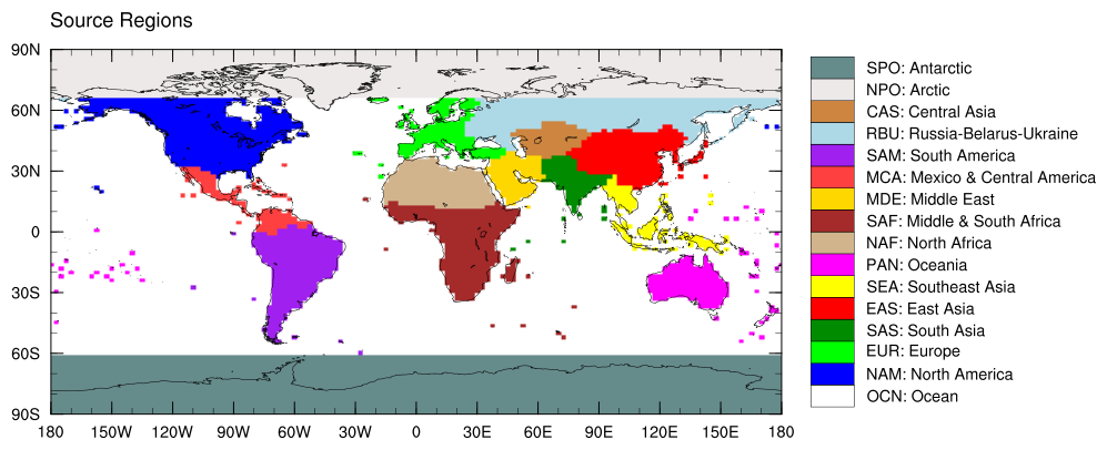
Figure 1 HTAP Tier 1 regions which form the basis for source regions for NO_x and VOC tagging. Oceanic tagged regions are shown in Fig. S12. More details on tagged regions are provided in Table 1.

Table 1 Various emission tags for NO_x- and VOC-tagged simulations. The geographic definition of the land-based tags corresponds to the HTAP tier 1 regions as shown in Fig. 1. For NO_x-tagging, “Rest of the World” corresponds to the tier 1 regions of South America, Oceania, and Middle and Southern Africa combined. For VOC-tagging, the regions: Arctic, Central Asia, Mexico and Central America, North Africa, and Southeast Asia were also combined into the “Rest of the World”. The regional oceanic tags are only applicable for NO_x-tagging and their geographic definitions are shown in Fig. S12. For VOC-tagging we use a single oceanic tag representing NMVOCs from shipping and natural DMS emissions. Lightning tag is only applicable for NO_x-tagging.

We specify an additional tag for NO_x emission generated from lightning parameterization (Price and Rind, 1992; Price et al., 1997) in our NO_x-tagged simulation, and for methane in our VOC-tagged simulation. We refer the reader to Fig. 1 for the geographic definitions of the various source regions and to Table 1 for more details on the regional and global tags for the NO_x and VOC-tagging runs. Based on these tags changes were made to the model source code following Butler et al. (2018) which allows for physical and chemical treatment of all tagged species within the model.

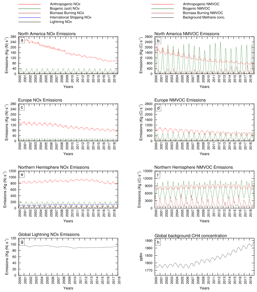
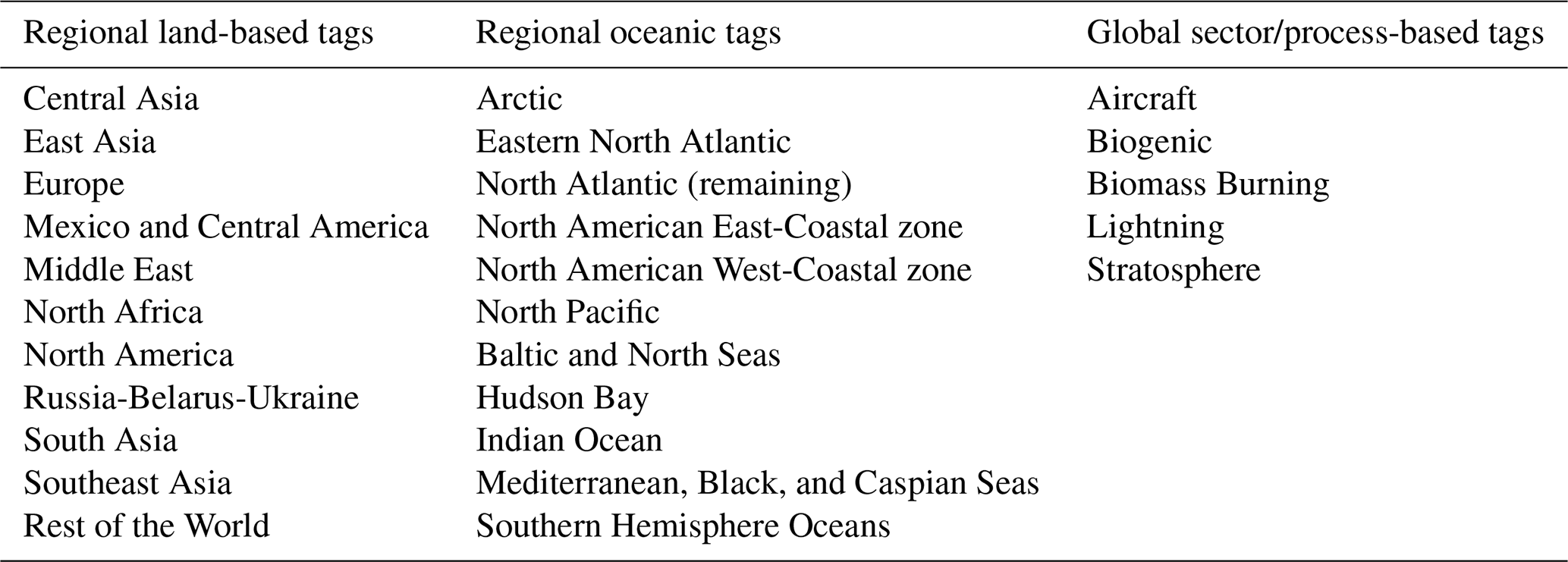
Figure 2 Time-series of NO_x- (left panels) and VOC-emissions (right panels) for North America (a, b), and Europe (c, d) source regions along with Northern Hemispheric totals (e, f) and global totals of lightning NO_x and background CH₄ concentrations over the study period.

Figure 2 shows the trends in NO_x and VOC emissions for North America (NAM) and Europe (EUR) tagged source regions and for the northern hemisphere along with the global lightning NO_x emissions and prescribed methane concentrations over the study period. We see a consistent decline in North American anthropogenic NO_x emissions (Fig. 2a) from $\sim \mathrm{250}\mathrm{kg}\left(\mathrm{N}\right){\mathrm{s}}^{-\mathrm{1}}$ in 2000 down to $\sim \mathrm{100}\mathrm{kg}\left(\mathrm{N}\right){\mathrm{s}}^{-\mathrm{1}}$. We also see a decline in European anthropogenic NO_x emissions (Fig. 2c), although starting from a lower base in 2000, from $\sim \mathrm{140}\mathrm{kg}\left(\mathrm{N}\right){\mathrm{s}}^{-\mathrm{1}}$ down to 80 kg (N) s⁻¹. Similarly, the anthropogenic NMVOCs, or AVOCs, in the two regions (Fig. 2b and d) have also declined substantially. These large emission changes reflect the strict and effective emission control policies implemented in these regions (Clean Air Act, 1963; Clean Air Act Amendments, 1990; Council Directive, 1996, 2008). The biogenic NO_x emissions peak in summertime for both regions but remain much lower (up to 40 kg (N) s⁻¹ in North America and 20 kg (N) s⁻¹ in Europe) than the anthropogenic NO_x emissions and exhibit no long-term trend. NO_x emissions from fires remain extremely small. The biogenic NMVOCs, or natural VOCs, also peak during summertime for both regions. This is due to the larger leaf area in the summer season (Guenther et al., 2006; Lawrence and Chase, 2007). The natural VOCs for North America are higher than the AVOCs and show an increasing trend since 2013. The natural VOC emissions in Europe are comparable to the AVOC emissions especially in recent years. The biomass burning NMVOC emissions are the smallest but they show an increasing trend in North America. We have also plotted the total northern hemispheric (NH) NO_x and NMVOC emissions which can provide some context in understanding foreign contributions to ozone in North America and Europe. Here, we see the NH anthropogenic NO_x increasing from 2000 until 2013 after which it declines to below 2000 levels. This increasing trend is primarily driven by increasing Chinese emissions, while the decline is driven by a decline in Chinese, North American and European emissions (not shown). We see a similar trend for NH AVOC as well. Summertime NH natural VOC emissions exceed the AVOC emissions. NH biomass burning NMVOC emissions are also significant, up to 5000 kg C s⁻¹, but they are lower than natural VOC and AVOC emissions and do not show any significant trend. Global lightning NO_x emissions show a declining trend from $\sim \mathrm{100}\mathrm{kg}\left(\mathrm{N}\right){\mathrm{s}}^{-\mathrm{1}}$ in 2000 to $\sim \mathrm{90}\mathrm{kg}\left(\mathrm{N}\right){\mathrm{s}}^{-\mathrm{1}}$ in 2014 after which they increase to 95 kg (N) s⁻¹ in 2018. The global methane concentration remains consistent, around 1780 ppb, for 2000–2006 but rises steadily since 2007 reaching around 1880 ppb in 2018. Understanding these trends in regional emissions of different ozone precursors allows us to better interpret tagged contributions to simulated ozone in later sections.

2.2 Model runs and initial post-processing:

We perform two separate 20 year long simulations for 1999–2018. The first year, 1999, is discarded as a spin-up year and only the outputs for 2000–2018 are used for further analyses. For the VOC-tagged run, the spin-up time was two years, such that the 1999 run was restarted with the conditions at the end of the first 1999 run. Introducing extra tagged species with full physical and chemical treatment in the model leads to a substantial increase in computational time (approx. $\mathrm{6}\times -\mathrm{8}\times$) as compared to a basic model run without tagging. Therefore, such a model configuration typically needs a large number of CPU cores spread over multiple parallel nodes. We run our tagged simulations on 6-nodes with 72 Intel Icelake cores each (432 cores in total) with a memory of 2048 GB per node. It takes approximately 24 and 36 h wallclock time to complete a single year of simulation with NO_x- and VOC-tagging, respectively, with our model configuration. The VOC-tagged simulations take longer despite having fewer land-based and oceanic tags because, unlike NO_x-tagging, VOC-tagging involves all speciated NMVOCs to be tagged separately thereby increasing the total number of chemical species to be treated in the model.

We configure the model to write out key meteorological and chemical variables, including tagged O₃ variables, as 3D output at monthly average frequency but also write out the tagged O₃ variables at surface at an hourly frequency which allows us to assess key policy-relevant ozone metrics for further analyses. Before we proceed to analyses of the results, we convert the model output into global MDA8 O₃ (maximum daily 8 h average) values along with its tagged contributions for each grid cell in the model. The model writes-out the hourly ozone values in Universal Time Coordinates (UTC) for all locations. Therefore, we first, consider different time-zones (24 hourly zones based on longitude range) and select the 24 ozone values by applying the appropriate time-offset to reflect a “local day” for each grid cell. Once a 24 h local-day has been selected, we perform 8 h running averages spanning these 24 values and pick the maximum of these 8 h averages as the MDA8 O₃ value for that grid cell on a given day. We then use the selected time window for the MDA8 O₃ value for the grid cell to also calculate the 8 h-average tagged contribution over this window. Using this methodology, we prepare global NetCDF files which contain daily MDA8 O₃ values along with tagged contributions for each grid cell. We use these files for further analyses.

Figure 3 shows the geographic definitions of various HTAP-Tier 2 regions (Galmarini et al., 2017), out of which nine regions, five in North America, namely Eastern Canada, Northwest United States (NW US), Southwest United States (SW US), Northeast United States (NE US), and Southeast United States (SW US), and four in Europe,namely Western Europe, Southern Europe, C&E Europe, and SE Europe, shown in various shades of magenta and green, are used as receptor regions to perform further analyses of trends and seasonality in Sect. 3. We use these receptor regions to perform area-weighted spatial averaging of MDA8 O₃ values before analysing the trends and contributions. Area-weighted spatial averaging is needed because different model grid cells cover different areas on the ground based on the rectangular lat-long coordinate system, with high-latitude grid cells covering smaller areas and low-latitude and equatorial grid cells covering larger areas. So, a simple spatial averaging will overrepresent the concentrations of high-latitude gridcells and underrepresent lower-latitude gridcell concentrations in the receptor region average. So, we derive dimensionless coefficients for all grid cells within each receptor region based on their relative size to the average grid cell area in that region. We scale the gridded MDA8 O₃ with these area-coefficients before spatial averaging, ensuring a proportionate representation of the MDA8 O₃ value over the entire receptor region.

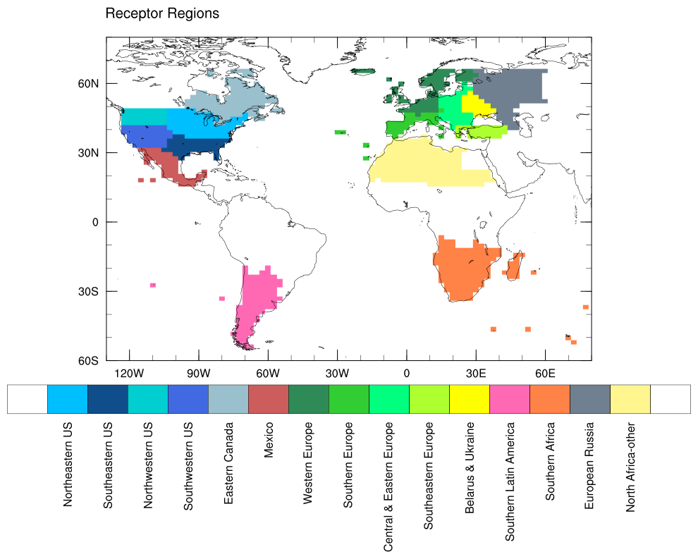
Figure 3 Receptor regions considered for model evaluation or analysis. Note that many regions were sparsely sampled due to lack of a wide rural observational network within these regions.

2.3 TOAR Observations and related data processing:

For model evaluation, we utilize ground-based observations of hourly ozone from many stations over North America and Europe which are part of the TOAR-II database of the Tropospheric Ozone Assessment Report (TOAR). We use the newly developed TOAR gridding tool (TOAR Gridding Tool, 2024) to convert the point observations from individual stations into a global gridded dataset which matches our model resolution of 1.9°×2.5°. The TOAR gridding tool allows for data selection including the variable name, statistical aggregation, temporal extent and a filtering capability according to the station metadata.

We extract the Maximum Daily 8 h Average (MDA8) metric for ozone from the TOAR-II database analysis service (TOAR-II, 2021) for the years 2000–2018 (as available until May 2024). The MDA8 values are only saved if at least 18 of the 24 hourly values per day are valid (see, dma8epa_strict in TOAR-analysis, 2023). This allows us to minimize any discrepancies between the observed and model-derived MDA8 O₃ values. Also, since our model resolution is coarse, we only include rural background stations in our analyses to avoid influences of urban chemistry which may not be resolved in our model.

We use the type_of_area field of the station metadata to select the rural stations; this information is provided by the original data providers (see Acknowledgements for an exhaustive list of data providers). They cover about 20 % of all stations in North America and Europe. We note that roughly a similar fraction of stations in these regions remains unclassified. In the final gridded product, which contains daily MDA8 O₃ values over North America and Europe a grid cell has non-missing value if there is at least one rural station present within it. We obtain large parts of NAM and EUR regions with valid TOAR grid cells, although the number of these valid grid cells changes day-to-day and year-to-year. In North America, the number of valid stations varies from 3–4 for Eastern Canada, 17–34 for NW US, 53–139 for SW US, 178–207 for NE US, 116–139 for SE US. In Europe, the number of rural stations varies from 140–154 for Western Europe, 50–185 for Southern Europe, 36–86 for C&E Europe, and 1–19 for SE Europe, with a general increase in the number of stations in each region with time. Furthermore, the number of valid TOAR stations within each grid cell also varies for certain locations. To better understand the changes in the TOAR station network in each of the 9 receptor regions considered here, we have plotted a time-series of annual average number of stations within each receptor region. This is shown in Fig. S14. We note that sparse spatiotemporal sampling can introduce uncertainty in identifying true long-term trends of ozone and refer the reader to a technical note on this issue by Chang et al. (2024) for more details.

3 Results

3.1 Model evaluation

The CAM4-Chem model has been evaluated for its ability of simulating the distribution and trends of tropospheric ozone by many previous studies (Lamarque et al., 2012; Tilmes et al., 2015) including its modified version with ozone tagging (Butler et al., 2020; Nalam et al., 2025). Generally, many atmospheric models including CAM4-Chem have been shown to overestimate surface ozone in the Northern Hemisphere (Reidmiller et al., 2009; Fiore et al., 2009; Lamarque et al., 2012; Young et al., 2013; Tilmes et al., 2015; Young et al., 2018; Huang et al., 2021). In a recent study that utilized the same model simulations as those presented in this study, Nalam et al. (2025) evaluated model simulated monthly average surface ozone against gridded observations from the TOAR-I dataset (Schultz et al., 2017) over various HTAP Tier 2 regions (Galmarini et al., 2017) in North America, Europe and East Asia for 2000–2014 and found a satisfactory performance, albeit with a general high bias of 4–12 ppb, similar to a reference CMIP6 model CESM2-WACCM6 (Emmons et al., 2020); see Fig. 1 in Nalam et al., 2025 for more details. Furthermore, Nalam et al. (2025) have also evaluated the model simulated monthly mean ozone against the ozone sonde-based climatology compiled by Tilmes et al. (2012) for different latitude bands in the northern hemisphere at different pressure levels over the same period and found generally high correlations and low biases – see Fig. 2 in Nalam et al. (2025) for further details.

One reason for a high bias as seen in Nalam et al. (2025) and other studies could be the use of all available stations (including many urban stations) for evaluating the model performance. Given the coarse model resolution, we expect the model not to resolve high NO_x concentrations around the urban and industrial centres and therefore suffer from the lack of ozone titration. Therefore, here, we only evaluate the model against data from rural stations, wherever available. Also, in this study, we only work with policy-relevant metrics such as Maximum Daily 8 h Average (MDA8) Ozone at the surface or other metrics derived from it, e.g., Peak Season Ozone (PSO). These metrics generally include only the daytime ozone, especially over land. Therefore, evaluating the model for these metrics also allows us to exclude nighttime ozone and avoid any large nighttime biases which often arise due to improper simulation of the nighttime boundary layer which has been a persistent issue in both global and regional models (Houweling et al., 2017; Du et al., 2020; Ansari et al., 2019).

For model evaluation, we derive regionally averaged monthly mean MDA8 O₃ for all HTAP tier 2 receptor regions for North America (except Western Canada) and Europe but sample the MDA8 O₃ values only from those gridcells where rural TOAR observations were available. Figure 4 shows the time-series of monthly mean MDA8 O₃ from the model and TOAR observations for the entire simulation period. We ask the reader to refer to the geographic extent of the receptor regions discussed here in Fig. 3. We do not include model evaluation results for Western Canada due to the unavailability of rural observations from this region in the TOAR-II gridded dataset. While some rural observations exist for this region, the essential rural/urban classification was not included by the original data providers which hindered us from utilizing these observations for model evaluation. We emphasize the importance of including all essential station metadata so that the observations are well-utilized by other researchers in future studies. Evaluation for more regions in other continents are provided in the Supplement (see Fig. S1).

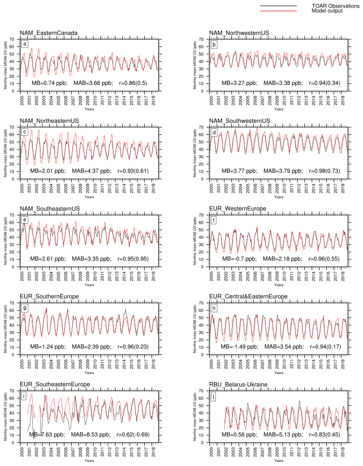
Figure 4 Time series of observed versus simulated monthly mean MDA8 O₃ along with mean bias, mean absolute bias, and correlation coefficients for various receptor regions. Correlation coefficients for annual averaged data are mentioned in brackets. Only rural stations data were utilized from the TOAR database and model output was fetched only for those grid cells where observations were available.

In Eastern Canada (Fig. 4a), the model reproduces the O₃ seasonal cycle very well, especially between 2007–2018. It overshoots the maxima and undershoots the minima for the earlier years of 2000–2006. This could be due to inaccurate (higher) NO_x emissions over the region in the HTAPv3 inventory for the earlier years which leads to higher summertime production and lower wintertime levels due to increased titration. The model also reproduces the flattening annual cycle well which is consistent with decreasing NO_x emissions over this region (see Figs. 3 and S6). For the Northwestern United States (Fig. 4b), the model reproduces the annual cycle well, although it systematically overestimates the MDA8 O₃ during peak season by up to 5 ppb. For the Northeastern United States (Fig. 4c), the model captures the structure of the annual cycle of MDA8 O₃ very well for recent years but overestimates the summer peak and underestimates wintertime ozone for earlier years, similar to Eastern Canada, again pointing to high NO_x emissions in the emission inventory over this region in the initial years. The model shows an extremely skilful simulation of MDA8 O₃ in the Southern United States. In SW US (Fig. 4d), the model reproduces the gradual and steady decline in MDA8 O₃ over time, albeit with a slight overprediction (∼2 ppb) in later years. Similarly, in the SE US (Fig. 4e), we note a very good reproduction of trends, with a decreasing summertime peak. For all North American regions, we see a high correlation between observed and modelled monthly mean MDA8 O₃ values with correlation coefficient r ranging from 0.86–0.98. Correlations at the annual average timescale are lower (0.34–0.95) and driven by interannual variability rather than seasonality of ozone. Mean bias is positive for all regions and ranges from 0.68–3.65 ppb. Mean absolute bias ranges from 3.35–4.37 ppb.

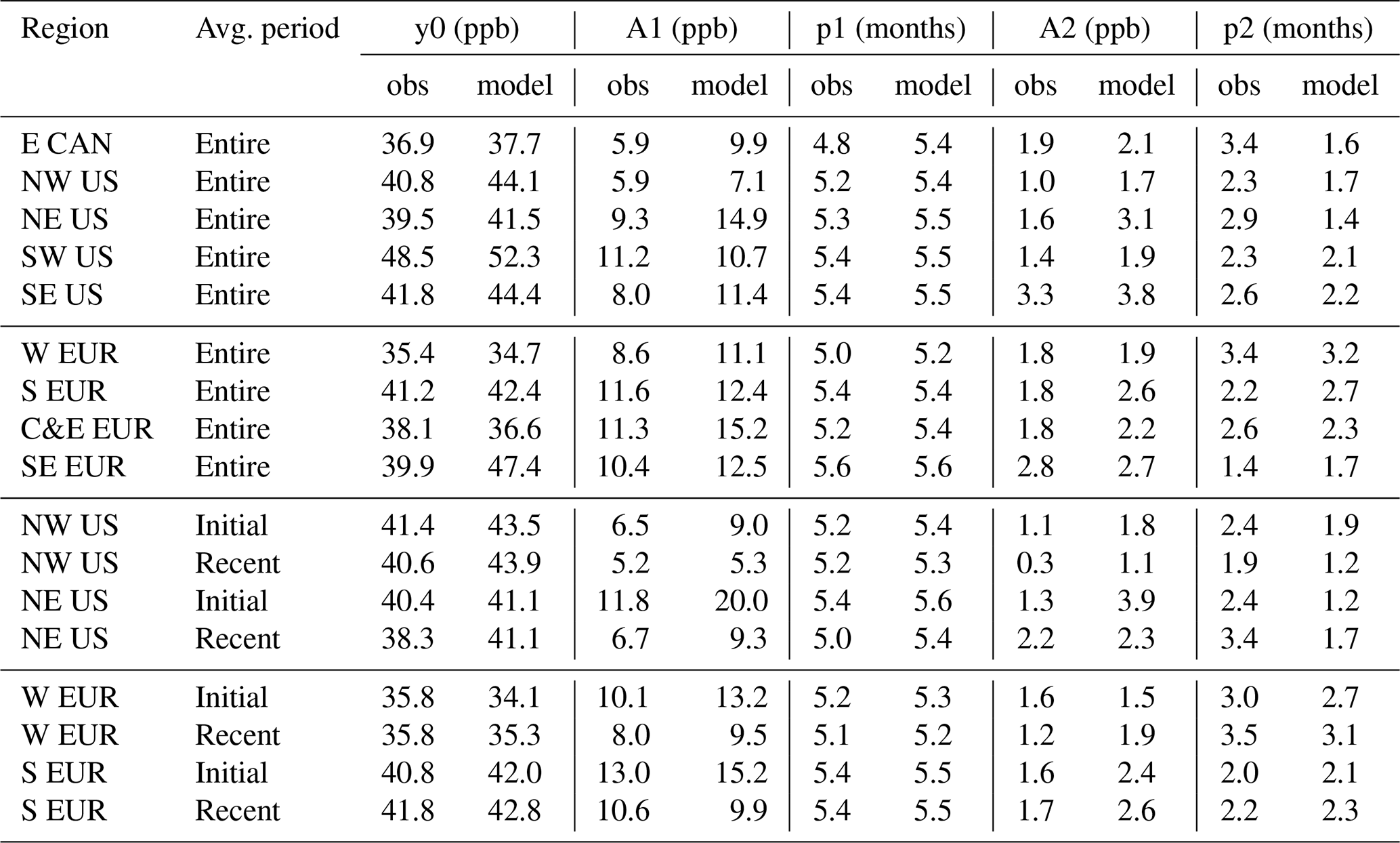
Since the MDA8 O₃ seasonal cycle is a subject of further analysis in this study and forms a key part of our results, it is imperative to perform a more rigorous evaluation of the model's ability to capture its various features quantitatively. Parrish et al. (2016) provide a good precedent for such an evaluation where they break down the observed and modelled ozone seasonal cycle into a y intercept (annual average) and two sinusoidal harmonics using a Fourier transform and then statistically compare the fit parameters that define these harmonics (i.e. amplitudes and phase angles) for the observed and modelled data. They argue that the first harmonic, with its large amplitude and phase angle, broadly represents the local photochemical production of ozone, while the generally out-of-phase second harmonic, with a smaller amplitude and phase angle, is related to the photolytic loss of O₃, driven by j(O¹D) – a hypothesis supported by the finding that the second harmonic is small in the free troposphere but grows more significant in the marine boundary layer (MBL), at least for alpine and remote sites analyzed (Parrish et al., 2020). Thus comparing these Fourier parameters for the observed and modelled data can unveil specific model skill or lack thereof in capturing different aspects of atmospheric chemistry which ultimately determine the shape of O₃ seasonal cycle (Bowdalo et al., 2016; Parrish et al., 2016; Bowman et al., 2022). We performed a quantitative evaluation of the seasonal cycles following a similar approach. A short technical description of the Fourier decomposition is provided in Sect. S2. Figure S4 presents scatterplots for these five essential fourier parameters, y0 in ppb (y intercept representing annual average MDA8 O₃), A1 in ppb (amplitude of the first or fundamental harmonic), p1 in months (phase peak of the fundamental harmonic), A2 in ppb (amplitude of the second harmonic), and p2 in months (phase peak of the second harmonic). In terms of y0, the correlation coefficient r ranges from 0.34 to 0.95 for the five North American receptor regions considered and is 0.97 for all five regions combined, with higher values for southern US but lower values for NW US and Eastern Canada, reflecting lower model skill in capturing the interannual variability of MDA8 O₃ in these regions. The model is more skilful in capturing the amplitude of the fundamental harmonic (r values from 0.72–0.93; 0.74 overall) than in capturing the amplitude of the second harmonic (r values from 0.09–0.90; 0.52 overall). In terms of phase peaks too, the model is more skilful in capturing the phase peaks for the fundamental harmonic (r values from 0.63–0.93; 0.83 overall) than for the second harmonic (r values from 0.41–0.74; 0.30 overall). The model generally overestimates y0, A1, A2, and p1 but underestimates p2. In general we can state that the first harmonic which is related to local photochemistry is well captured by the model for most of North America. The second harmonic, in our case, might be related to all other processes that modify the near-sinusoidal shape of the O₃ seasonal cycle (e.g., long range transport of ozone from other regions and from stratosphere and photolytic losses), and these processes are relatively less well captured by the model. All Fourier fit parameters for the observed and modelled MDA8 O₃ seasonal cycles have been tabulated in Tables S1–S5 in the Supplement for different North American receptor regions.

The model reproduces the monthly mean MDA8 O₃ for Europe extremely well with very small mean biases (−1.54–1.25 ppb), small mean absolute biases (2.18–3.54), and very high r values ranging from 0.94–0.97 (0.17–0.55 for annual averaged timescale) for various regions, except SE Europe and RBU region. For Western Europe (Fig. 4f), it captures both the trends and the structure of the seasonal cycle extremely well, for example, note the near-stagnant maxima and increasing minima over time in both observations and model output. Similarly for Southern Europe (Fig. 4g), we again see a very skilful simulation of monthly mean MDA8 for the entire simulation period – this includes capturing the slightly decreasing summer maxima and increasing winter minima and an overall flattening of the seasonal cycle post 2006. We see a very good reproduction of MDA8 O₃ for C&E Europe (Fig. 4h) particularly for the summer months. We see a small underprediction for the winter months in years up to 2012. However, it is the summertime MDA8 O₃ values that constitute the peak season ozone metric which are ultimately utilized in our further policy-relevant analyses. Finally, for SE Europe (Fig. 4i), we notice an overprediction of MDA8 O₃ for early years, until 2006, after which the model captures the trends and particularly the summer peaks very well. The mean bias is 7.63 ppb and r value is 0.62.

Similar to North America, we also performed a Fourier transform analysis for European regions which provides a quantitative basis for assessing model skill in reproducing various aspects of the MDA8 O₃ seasonal cycle across the 19 year study period. Scatterplots in Fig. S5 show high correlations between observed and modelled amplitudes ($r=\mathrm{0.79}-\mathrm{1.0}$ and 1.0 overall for A1; and 0.62–1.0 and 1.0 overall for A2) and phase peak timings for both harmonics ($r=\mathrm{0.73}=\mathrm{0.92}$ and 0.91 overall for p1; $r=\mathrm{0.33}-\mathrm{0.96}$ and 0.73 overall for p2). The general high biases, as seen in North American regions, are also not present except for the first harmonic parameters for Western Europe and C&E Europe. This highlights a very high model skill in reproducing the fundamental local ozone photochemistry as well as transport and loss processes in Europe. The y intercept y0, representing interannual variability of ozone, shows lowest correlations ($r=-\mathrm{0.29}-\mathrm{0.55}$ and 0.31 overall) which suggests that year-to-year meteorological changes remain a source of model bias and uncertainty in this region. All Fourier fit parameters for the observed and modelled MDA8 O₃ seasonal cycles have been tabulated in Tables S6–S9 for different European receptor regions.

We have also included the Belarus and Ukraine region (Fig. 4j; with 1–2 valid stations) in our evaluation and here too we see a good simulation of MDA8 O₃ for the entire period, with a small mean bias of 0.56 ppb and r value of 0.83 at monthly timescale and 0.45 at annual averaged timescale, barring a couple of years (2014 and 2017) when the model overestimates the values. We have also evaluated the model for MDA8 O₃ against rural observations from the TOAR-II database in other regions including Mexico (11–14 stations), North Africa (1–3 stations), Southern Africa (1 station), Southern Latin America (1–2 stations), and European Russia (2 stations; see Fig. 3 for region definitions), where the model has also captured the trends well, however, since we do not discuss these regions in further analyses, they are presented in the supplement (see, Fig. S1). Here too, the model output is extracted only from those grid cells where at least one TOAR station exists, ensuring representative co-sampling.

We also evaluate the model in the context of potential overestimation of ozone production from ship plumes. This is because in our modelling setup, ship NO_x emissions are instantaneously diluted within the 1.9°×2.5° model grid cell which can lead to an overestimation of ozone production efficiency from ship NO_x. In the real world, the more localized, high-NO_x conditions within a concentrated young plume, the titration effects and NO_x self-reactions can be more dominant and the true ship NO_x contribution might be somewhat lower than simulated (Kasibhatla et al., 2000; Chen et al., 2005; Huszar et al., 2010). Such overestimated ship NO_x contribution to ozone shows up, for example, in terms of a lower simulated vertical gradient than the observed vertical profile of ozone especially at remote coastal locations. To assess this, we plot observed and model simulated ozone vertical profiles at Trinidad Head, off the coast of California, for the month of July (a representative month for peak season) for all 19 years (see Fig. S6). The monthly mean modelled vertical O₃ profile over Trinidad Head generally falls within the envelope of daily observational profiles within the MBL (say, below 850 hPa). Although, for multiple years, the vertical drop in modelled O₃ concentration towards the surface is less sharp than that seen in observations, thereby suggesting a potential overproduction of O₃ near the ocean surface in the model due to instantaneous distribution of ship NO_x emissions in the model gridcell. We also performed a zero-order sanity check by comparing the inferred ozone production rate from ship NO_x within the marine boundary layer of the northern hemisphere midlatitude region in the model with observational values. We found a potential overproduction of ozone by ships in the model by a factor of 3.3 when compared to the data from previous observational studies. We refer the reader to Sect. S1 in the Supplement for a detailed discussion on these calculations. This particular feature of our modelling system can partly explain the positive bias in simulated ozone.

Overall, we obtain very good model-observations agreement, with low biases and high correlations, better than previous studies (e.g., Butler et al., 2020; Li et al., 2023; Garatachea et al., 2024). The possible reasons for such improved performance could be (1) the use of the newly developed HTAPv3 emissions inventory (2) using only rural stations for evaluation which avoids urban titration which may be present in the observations but not in model output (3) improved treatment of spatial and temporal representativeness (including the treatment of missing values) of the stations through the TOAR gridding tool (4) evaluating the policy-relevant MDA8 O₃ metric which avoids nighttime O₃ which may not be well-simulated due to improper estimation of the nighttime boundary layer. We note that our model evaluation is based on model results and observations of time series of MDA8 O₃ that are averaged, both temporally (monthly) and spatially (first over model grid cells and then over receptor regions) but such an evaluation is valid because all our subsequent analyses and conclusions depend on the same spatial and temporal scales. We note that agreement between models and observations does not in itself demonstrate that the models represent all processes correctly, since models are necessarily simplified representations of reality and can reproduce certain features for the “wrong” reasons. As Box (1976) succinctly put it, “all models are wrong, but some are useful”; our comparisons should therefore be viewed in this light.

After a satisfactory performance of the model across different world regions and, in particular, excellent performance in the simulation of MDA8 O₃ against rural stations from the TOAR-II database, we proceed to further analyses of trends and source contributions to ozone in different receptor regions. First, to explain the year-to-year trends, we present the full 19 year time series of Peak Season Ozone (PSO) for North America and Europe along with their NO_x- and VOC- source contributions derived from our two tagged simulations. After explaining the year-to-year trends in ozone in terms of the NO_x and VOC contributions, we further calculated a 19 year month-centered average MDA8 O₃ and its source contributions for each receptor region. This allows us to interpret the leading sources of ozone in each receptor region on a monthly basis averaged over the entire simulation period. We also present the first five year (2000–2004) and last five year (2014–2018) month-centered average MDA8 O₃ seasonal cycle and explain the shifts in terms of tagged contributions for all receptor regions during these periods. In the next Sections, we present these results for North America and Europe.

3.2 Ozone in North America

3.2.1 Peak season ozone in North America: regional trends and source contributions

In this section we discuss the trends in and contributions to PSO in North America. The Peak Season Ozone for any location is defined as the highest of the 6 month running average of monthly mean MDA8 O₃ values. In order to compute PSO, we performed the averaging over 6 month windows (January–June, February–July, March–August and so on) over the TOAR observations and the same time window was imposed over the modelled values for calculating the 6 month averaging (instead of independently selecting the peak 6 month time window for the model). This approach ensures temporal consistency between the observations and modelled values. Furthermore, for spatial consistency, the model values were sampled only from those grid cells where at least one TOAR-II station was present. Finally, these values from multiple grid cells were spatially averaged over various receptor regions after weighting them with the grid cell areas to derive a single PSO value per region per year for observations and the model along with tagged contributions.

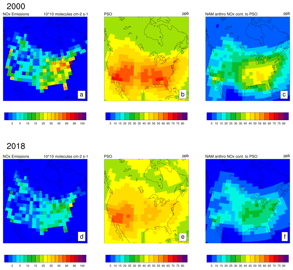
Figure 5 Spatial distribution of local anthropogenic NO_x emissions during peak season (a, d), PSO (b, e), and local anthropogenic NO_x contribution to PSO (c, f) for North America during the initial (2000) and final year (2018). Here, emissions for each grid cell were calculated by averaging over a 6 month time window that matches the PSO window over the grid cell.

Before examining the detailed temporal trends and source contributions to PSO in specific North American receptor regions, it is instructive to visualize the spatial distribution of NO_x emissions and their impact on PSO. Figure 5 illustrates the gridded local anthropogenic NO_x emissions (panels a and d), the total modelled PSO (panels b and e), and the modeled contribution of local anthropogenic NO_x to PSO (panels c and f) for the initial (2000) and final (2018) years of our analysis. The NO_x emissions, for each grid cell, are calculated for the same 6 month window as the PSO for the grid cell. In 2000 (Fig. 5a), high NO_x emissions were concentrated over the Eastern United States, particularly the Ohio River Valley and the Northeast corridor, as well as in California and other major urban centers. By 2018 (Fig. 5d), these emissions had substantially decreased across most of the continent, with the most dramatic reductions evident in the aforementioned historical hotspot regions. This widespread decline in local NO_x emissions directly translated to changes in ozone levels. The spatial distribution of total PSO (Fig. 5b and e) shows a corresponding general decrease between 2000 and 2018, particularly in the eastern and central US. The spatial features of PSO for both years are very similar to bias-corrected maps of PSO for 2000 and 2017 presented in Becker et al. (2023). More specifically, the contribution of local anthropogenic NO_x to PSO (Fig. 5c and f) shows a marked reduction in magnitude across the continent. In 2000, local NO_x contributed significantly to PSO over large swathes of the eastern and southern US, whereas by 2018, this direct local contribution had diminished considerably, becoming more confined to residual emission hotspots. These spatial changes provide a crucial backdrop for understanding the regionally averaged trends discussed below.

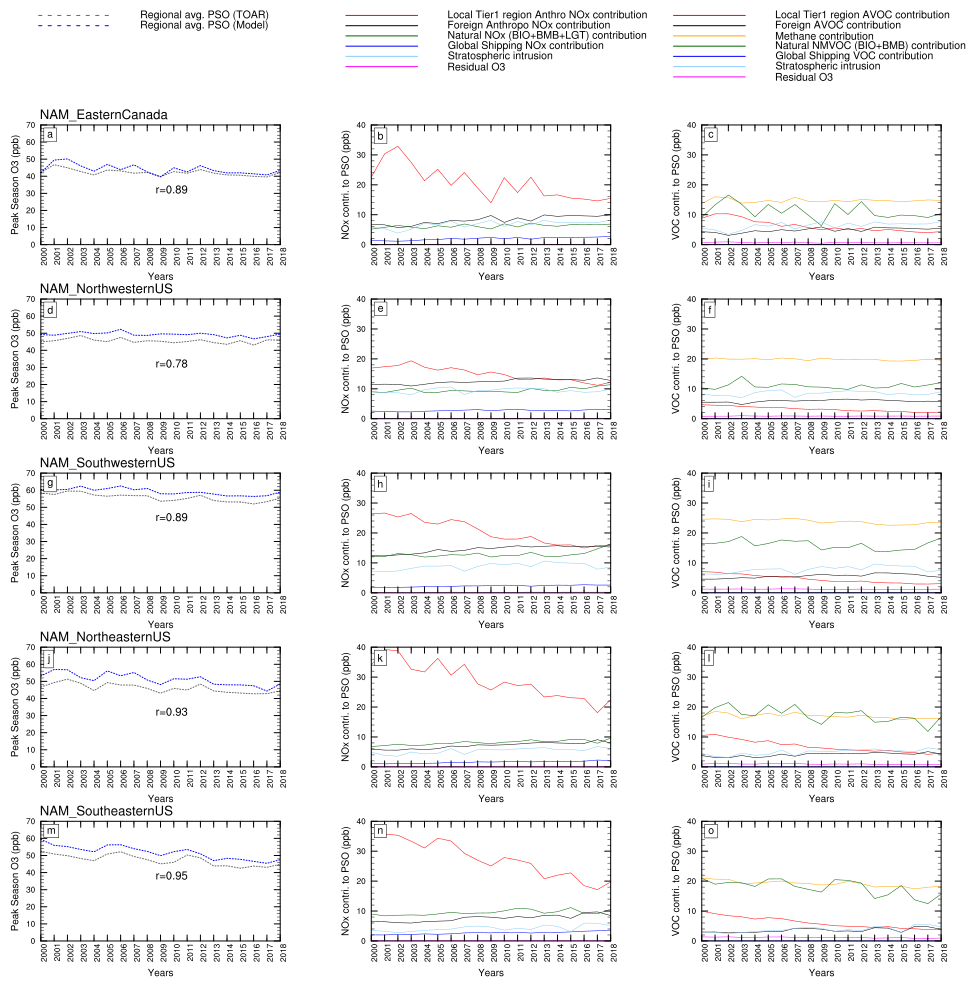
Figure 6 Time-series of observed and model-derived Peak Season Ozone for various receptor regions in North America for 2000–2018 (left panels) and its source contributions in terms of NO_x sources (middle panels panels) and VOC sources (right panels). Model output was sampled from TOAR-valid grid cells only.

Figure 6 presents the time series of observed and model-simulated total PSO (panels a, d, g, j, m), alongside the attributed contributions from NO_x sources (panels b, e, h, k, n) and VOC sources (panels c, f, i, l, o). On a visual inspection of observed and modelled PSO trends (left column panels) we decided to fit Generalized Least Squares (GLS) linear trends to these data points. We note that some previous studies have fitted higher order functions to ozone data over North America as necessitated by their longer period of analysis where ozone concentrations increased, stagnated, and then decreased (Logan et al., 2012; Parrish et al., 2025; Parrish et al., 2020). However, a linear fit is appropriate for the period considered in this study when local emissions have only declined (Fig. 2). Quantitative details of the trends and their significance for all contributions are provided in Table 3. Crucially, across all North American regions, the observed PSO levels consistently exceeded the WHO long-term guideline (31 ppb) by at least 10 ppb throughout the study period.

Observed PSO exhibits a decreasing trend in most North American regions (Fig. 6, panels a, d, g, j, m). For instance, Eastern Canada shows a slight decline ($-\mathrm{0.19}\left(\mathrm{0.01}\right)[-\mathrm{0.32},-\mathrm{0.06}]\mathrm{ppb}{\mathrm{yr}}^{-\mathrm{1}}$) [here and henceforth the trends are reported in the following format (trend (p-value) [95 % confidence lower limit, 95 % confidence upper limit])], while more substantial decreases are seen in the SW US ($-\mathrm{0.33}(<\mathrm{0.01})[-\mathrm{0.45},-\mathrm{0.21}]\mathrm{ppb}{\mathrm{yr}}^{-\mathrm{1}}$), NE US ($-\mathrm{0.34}(<\mathrm{0.01})[-\mathrm{0.50},-\mathrm{0.18}]\mathrm{ppb}{\mathrm{yr}}^{-\mathrm{1}}$), and SE US ($-\mathrm{0.46}(<\mathrm{0.01})[-\mathrm{0.63},-\mathrm{0.28}]\mathrm{ppb}{\mathrm{yr}}^{-\mathrm{1}}$). The NW US shows the smallest, albeit still decreasing, trend ($-\mathrm{0.09}\left(\mathrm{0.11}\right)[-\mathrm{0.20},\mathrm{0.02}]\mathrm{ppb}{\mathrm{yr}}^{-\mathrm{1}}$). The model generally captures these decreasing trends and the interannual variability reasonably well, though with some regional differences in magnitude: r-values between observed and modelled PSO are 0.89, 0.78, 0.89, 0.93, 0.93, and 0.95 and the difference in modelled and observed trends are −0.09, −0.02, 0.07, −0.16, and $-\mathrm{0.17}\mathrm{ppb}{\mathrm{yr}}^{-\mathrm{1}}$ for E Canada, NW US, SW US, NE US, and SE US, respectively. These regional differences in PSO trends are driven by regionally different local and remote contributions to PSO as revealed in Fig. 6.

The contributions from various NO_x sources show distinct regional patterns in their temporal evolution (Fig. 6, panels b, e, h, k, n; Table 3). The most significant driver of change is the local anthropogenic NO_x contribution, which has declined steeply across all regions, reflecting successful emission control policies. This decline is particularly sharp in the eastern US regions: NE US (from ∼35 ppb to ∼22 ppb; trend of $-\mathrm{0.97}(<\mathrm{0.01})[-\mathrm{1.19},-\mathrm{0.76}]\mathrm{ppb}{\mathrm{yr}}^{-\mathrm{1}}$) and SE US (from ∼38 ppb to ∼20 ppb; trend of $-\mathrm{1.09}(<\mathrm{0.01})[-\mathrm{1.25},-\mathrm{0.94}]\mathrm{ppb}{\mathrm{yr}}^{-\mathrm{1}}$). SW US also shows considerable decline in the local NO_x contribution (from ∼27 ppb to ∼16 ppb; trend of $-\mathrm{0.72}(<\mathrm{0.01})[-\mathrm{0.83},-\mathrm{0.62}]\mathrm{ppb}{\mathrm{yr}}^{-\mathrm{1}}$). Despite these reductions, local anthropogenic NO_x often remained a dominant contributor, especially in the earlier part of the study period, though its share has notably diminished. These results are consistent with findings from Simon et al. (2024) who analysed observational trends over 51 sites in the US over roughly the same period (2002–2019) and found the marked impact of clean air policies across the US such that the difference between the weekend (lower NO_x) and weekday (higher NO_x) MDA8 O₃ has diminished and become negative in recent years reflecting a transition from NO_x-saturated to NO_x-limited ozone formation regime.

Several previous observational-based studies have inferred the magnitude and temporal decline of local contributions to ozone in North America based on curve fitting the observed ozone time series data and have reported these magnitudes and e-folding times of the local ozone enhancements for various stations and regions (Parrish and Ennis, 2019; Derwent and Parrish, 2022; Parrish et al., 2025 among others). In order to facilitate a comparison with these observational studies, we also fitted an exponential function of the form shown in Eq. (1) to our model-derived local anthropogenic NO_x contributions to PSO for various receptor regions (see Fig. S16) and have tabulated the derived e-folding times against those found in literature (see Table S10). Here, A represents the magnitude of local NO_x contribution to PSO for the initial year (2000) in ppb and τ represents the e-folding time of these contributions. We find $\mathit{\tau }=\sim \mathrm{25}-\mathrm{38}\mathrm{yr}$ from the model and ∼22 yr from the literature for various US receptor regions.

$$\begin{array}{}\text{(1)}& y=A\exp \left(-{\displaystyle \frac{\mathrm{1}}{\mathit{\tau }}}t\right)\end{array}$$

To further quantify the relationship between these local emissions and their impact on ozone, we performed a gridded correlation analysis for the 2000–2018 period (Fig. 7). Figure 7a reveals the temporal correlation between local anthropogenic NO_x emissions and total PSO. Positive correlations are widespread, particularly strong ($r>\mathrm{0.6}-\mathrm{0.8}$) over much of the central and eastern US, indicating that in these locations, year-to-year variations in local emissions (i.e., their systematic decline) significantly drive the variability (decline) in total PSO levels. However, in other areas, such as parts of the western US and more remote regions, these correlations are weaker or even negative. This suggests a greater relative importance of factors like intercontinental transport of ozone and its precursors, or the influence of natural emissions, in driving total PSO variability in those areas, especially as local anthropogenic emissions have decreased.This lack of correlation between local NO_x emissions and observed MDA8 O₃ has been reported by Simon et al. (2024) for rural California even at a higher temporal frequency through disappearing day-of-week activity patterns indicating an increasing role of transported ozone in this region.

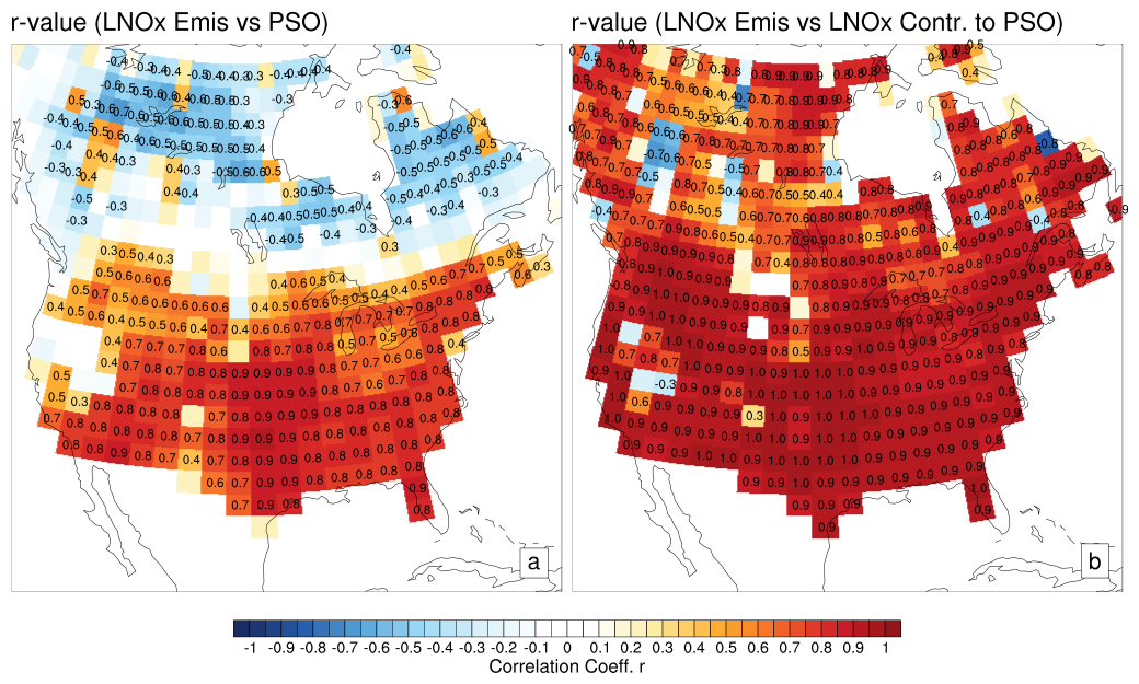
Figure 7 A spatial map showing correlation coefficient (r) between local (North American) anthropogenic NO_x versus PSO (a) and local anthropogenic NO_x versus local anthropogenic NO_x contribution to PSO (b) over the 19 yr for North America. For each year, and each gridcell, only peak season NO_x emissions were used.

More directly, Fig. 7b demonstrates a very strong and spatially ubiquitous positive correlation ($r>\mathrm{0.8}-\mathrm{0.9}$ in most populated areas) between local anthropogenic NO_x emissions and the modeled contribution of these local emissions to PSO. This high correlation validates that the model's attribution of ozone to local NO_x sources is directly and robustly responsive to changes in those local emissions themselves. It underscores that reductions in local NO_x emissions translate directly to reductions in the ozone specifically formed from those local emissions within the model framework. The slightly weaker correlations in very remote northern areas likely reflect the minimal anthropogenic emissions and thus lower signal-to-noise for this specific contribution. These spatial analyses highlight that while local NO_x emission reductions have been effective in decreasing their direct contribution to PSO across large areas, the impact on total PSO can be spatially heterogeneous due to the varying influence of other ozone sources and transport processes.

Conversely, the contribution from foreign anthropogenic NO_x (including aircraft) has generally increased across all regions (Fig. 6b, e, h, k, n; Table 3). This increase is most prominent in the western US regions. In the NW US, where its contribution has grown at $\mathrm{0.12}(<\mathrm{0.01})[\mathrm{0.09},\mathrm{0.16}]\mathrm{ppb}{\mathrm{yr}}^{-\mathrm{1}}$ (see Table 3) to become comparable to, and in recent years exceed, that of local anthropogenic NO_x. Similarly, in SW US, the foreign NO_x contribution has grown at $\mathrm{0.19}(<\mathrm{0.01})[\mathrm{0.15},\mathrm{0.24}]\mathrm{ppb}{\mathrm{yr}}^{-\mathrm{1}}$ to match the local NO_x contribution in recent years. Other regions like Eastern Canada and the NE US also show a discernible rise in foreign NO_x influence. The contribution from natural NO_x sources (biogenic, fire, and lightning) shows a slightly increasing trend in most regions (e.g., $\mathrm{0.12}(<\mathrm{0.01})[\mathrm{0.08},\mathrm{0.16}]\mathrm{ppb}{\mathrm{yr}}^{-\mathrm{1}}$ in NE US). This increase in contribution despite stable natural emissions (Fig. 2) indicates an enhanced ozone production efficiency from these natural NO_x sources in environments with lower overall anthropogenic NO_x levels, consistent with previous findings (e.g., Liu et al., 1987). Global shipping NO_x contributions, while smaller in absolute terms (typically $<\mathrm{2}-\mathrm{3}\mathrm{ppb}$), exhibit a consistent increasing trend across all receptor regions, reflecting rising emissions from this sector. Stratospheric intrusion provides a baseline ozone contribution with some interannual variability and small increasing trends in eastern regions (see Table 4).

The attribution of PSO to VOC sources (including methane) also reveals important trends and regional differences (Fig. 6, panels c, f, i, l, o; Table 3). Methane is consistently the largest single VOC contributor to PSO across most North American regions, typically contributing 15–25 ppb. Interestingly, despite the global increase in methane concentrations (Fig. 2 h), the methane contribution to PSO has remained relatively stable or even slightly decreased in some regions like the SW US ($-\mathrm{0.10}(<\mathrm{0.01})[-\mathrm{0.15},-\mathrm{0.06}]\mathrm{ppb}{\mathrm{yr}}^{-\mathrm{1}}$), NE US ($-\mathrm{0.09}(<\mathrm{0.01})[-\mathrm{0.15},-\mathrm{0.03}]\mathrm{ppb}{\mathrm{yr}}^{-\mathrm{1}}$) and SE US ($-\mathrm{0.15}(<\mathrm{0.01})[-\mathrm{0.20},-\mathrm{0.11}]\mathrm{ppb}{\mathrm{yr}}^{-\mathrm{1}}$). This is likely due to the reduced availability of local NO_x, which limits the efficiency of ozone production from methane oxidation. Contributions from local AVOC have generally declined across all regions, reflecting the reductions in their emissions as well as the local NO_x emission reductions. For example, the NE US saw a local AVOC contribution trend of $-\mathrm{0.36}(<\mathrm{0.01})[-\mathrm{0.41},-\mathrm{0.31}]\mathrm{ppb}{\mathrm{yr}}^{-\mathrm{1}}$, and the SE US experienced a similar decline ($-\mathrm{0.33}(<\mathrm{0.01})[-\mathrm{0.37},-\mathrm{0.29}]\mathrm{ppb}{\mathrm{yr}}^{-\mathrm{1}}$).

The role of natural VOCs (biogenic and fire) varies regionally. In forested regions like Eastern Canada and the NE US, natural VOCs make a substantial contribution (e.g., $\sim \mathrm{10}-\mathrm{18}\mathrm{ppb}$). The trend in their contribution is often negative (e.g., $-\mathrm{0.17}\left(\mathrm{0.10}\right)[-\mathrm{0.39},\mathrm{0.04}]\mathrm{ppb}{\mathrm{yr}}^{-\mathrm{1}}$ in Eastern Canada, $-\mathrm{0.24}\left(\mathrm{0.01}\right)[-\mathrm{0.42},-\mathrm{0.06}]\mathrm{ppb}{\mathrm{yr}}^{-\mathrm{1}}$ in NE US), which, similar to methane, may reflect the decreasing local NO_x rather than a decrease in natural VOC emissions themselves (which, for North America, Fig. 2 shows variability and some recent increases). For all regions, the year-to-year variability in local anthropogenic NO_x contributions often mirrors that of natural VOC contributions, suggesting strong chemical coupling between these local precursor pools. In arid regions like the NW US and SW US, the natural VOC contribution is understandably lower ($\sim \mathrm{14}-\mathrm{18}\mathrm{ppb}$ initially, declining) than the methane contribution. Contributions from foreign AVOCs, shipping VOCs, and stratospheric intrusion (VOC perspective) are generally smaller and show modest trends, with foreign AVOCs and stratospheric intrusion showing a slight increasing trend in some regions (see Table 3 for p-values and 95 % confidence intervals).

Our model-based findings of declining local anthropogenic contributions to PSO in North America differ quantitatively with recent observation-based studies such as Parrish et al. (2025), which also document a significant waning of local influence using different metrics and inferential techniques. For example, Parrish et al. (2025) estimate a local anthropogenic enhancement to Ozone Design Values (ODVs) in the SW US of typically <6 ppb in recent years. Our direct tagging method quantifies a larger local anthropogenic NO_x contribution to average PSO in this region (∼16 ppb in 2014–2018, Fig. 6 h). This quantitative difference likely arises from several factors. First, PSO represents a 6 month seasonal average of MDA8 O₃, while ODVs target specific high-percentile episodic conditions, and direct contributions to seasonal averages can be expected to differ from enhancements during specific episodes (although episodic contributions could be expected to have a higher share of local photochemistry than seasonal contributions). Second, and perhaps more fundamentally, inferential methods based on subtracting an estimated “baseline” from total observed ozone may systematically underestimate the full impact of local anthropogenic emissions. Such approaches often define the baseline based on remote sites or specific statistical filtering (e.g., Parrish et al., 2020), which may not fully account for the ozone produced from local emissions that is then regionally dispersed (as we also see indications of anthropogenic NO_x and BVOC interactions in the tagged output) or the non-linear chemical feedbacks that occur when local emissions are present. In contrast, our emissions tagging technique directly attributes ozone formation to its original precursor sources as they undergo transport and chemical transformation within the model's complete and consistent chemical framework. This provides a mechanistic quantification of source contributions to the specific PSO metric under baseline conditions. To ascertain this claim, we sampled the model output from the grid cells corresponding to these background stations (Trinidad Head for North America and Mace Head for Europe) and calculated the site-specific PSO and local anthropogenic NO_x contributions to PSO. These are reported in Table S11. As expected, we found that a significant portion of PSO at these background sites contains contributions from local NO_x emissions. For 2014–2018, we find the local contribution to PSO at Trinidad Head grid cell to be 4.0–6.6 ppb, which if added to the statistically-inferred local enhancement in SW US by Parrish et al. (2025) (6 ppb) would bring their values much closer to our findings (16 ppb). To facilitate better comparison with previous observational studies, we have also fitted a quadratic curve of the form $a+bt+c{t}^{\mathrm{2}}$, where t represents time in years, similar to Parrish et al. (2025), to the background contribution (sum of foreign anthropogenic NO_x, natural NO_x, and shipping NO_x) to PSO for SW US (see Table S12). We obtain parameter values of a=26.43 ppb, $b=\mathrm{0.08}\mathrm{ppb}{\mathrm{yr}}^{-\mathrm{1}}$, and $c=\mathrm{0.09}\mathrm{ppb}{\mathrm{yr}}^{-\mathrm{2}}.$ While inferential methods provide valuable observational constraints, our tagging approach offers a complementary, process-explicit view of how different sources contribute to the ozone burden in an evolving atmospheric environment.

In summary, declining PSO trends across North America are primarily driven by substantial reductions in local anthropogenic NO_x and, to a lesser extent, local AVOC contributions. However, these reductions are partially offset by increasing contributions from foreign anthropogenic NO_x, shipping NO_x, and, in some cases, an enhanced role of natural NO_x in ozone formation under lower ambient NO_x conditions. Methane remains a cornerstone of VOC-attributed ozone, but its contribution to PSO trends is heavily modulated by NO_x availability. The interplay between declining local NO_x and the ozone-forming potential of both natural VOCs and methane is a key feature influencing regional PSO trajectories. The NW US stands out as a region where foreign NO_x contributions now rival or exceed local sources, highlighting the growing importance of intercontinental transport for this region. Modelled PSO results for Western Canada are available in the Supplement (Fig. S7).

Table 2 Fourier analysis parameters derived from observed and modelled MDA8 O₃ seasonal cycle averaged over entire (2000–2018), initial (2000–2004), and recent (2014–2018) periods. Y0 denotes annual average MDA8 O₃, A1 and p1 denote the amplitude and phase peak of the first harmonic while A2 and p2 denote the amplitude and phase peak of the second harmonic.

3.2.2 Ozone seasonal cycle in North America: quantitative characterization and source contributions

To characterize the climatological seasonal cycle of MDA8 O₃ in North America and assess the model's ability to reproduce it, we performed a Fourier analysis (as detailed in Sect. 3.1) on the 19 year (2000–2018) averaged month-centered mean MDA8 O₃ time series for both observations and model output in each receptor region. This analysis decomposes the climatological seasonal cycle into its annual mean (y0), the amplitude (A1) and phase (p1) of the fundamental annual harmonic (related to local ozone photochemistry), and the amplitude (A2) and phase (p2) of the second harmonic (semi-annual cycle; related to long-range transport, stratospheric intrusion and loss processes). The phase p1 indicates the timing of the annual peak expressed in months, with numerically larger values typically corresponding to a later peak in the year (Bowdalo et al., 2016; Parrish et al., 2016; Bowman et al., 2022). These parameters are presented in Table 2 for averaged seasonal cycle and in Tables S1–S5 for individual years, while Fig. 8 illustrates the 19 year average seasonal cycle of total MDA8 O₃ and its attributed NO_x and VOC source contributions.

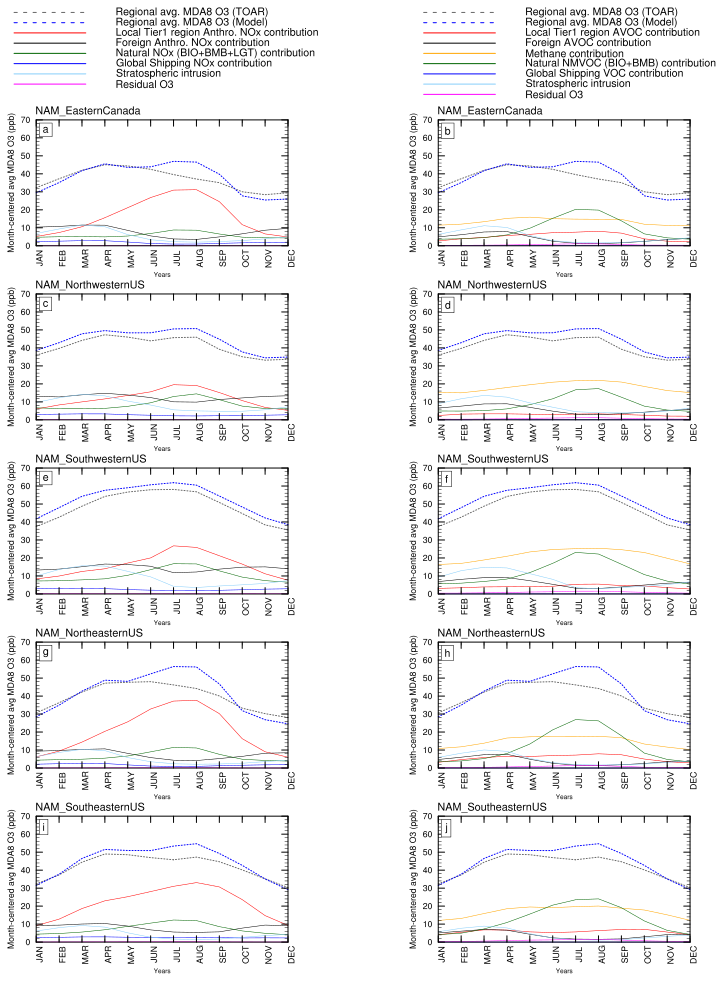
Figure 8 Month-centered average MDA8 O₃ over the 2000–2018 period for various receptor regions in North America and its source contributions in terms of NO_x sources (left panels) and VOC sources (right panels). Model output was sampled from TOAR-valid grid cells only.

The observed annual mean MDA8 O₃ (y0) varies across North American regions, ranging from approximately 37 ppb in Eastern Canada to a notably higher 48.5 ppb in the SW US, reflecting differing baseline ozone levels and regional influences (Table 2). The model generally captures these mean levels, though with a tendency for overestimation of 0.7–2.6 ppb in the eastern and 3.3–3.8 ppb in the western regions. This suggests a potential overestimation of background ozone or the combined influence of persistent remote/natural source contributions by the model in these regions. Figure 8c and e shows sustained contributions from foreign anthropogenic NO_x and methane in the NW US throughout the year, which could contribute to this higher baseline in the model but can only be ascertained via perturbation experiments which could be a topic of future studies

The amplitude of the primary annual cycle (A1) signifies the magnitude of the seasonal swing in ozone concentrations. Observed A1 is largest in the SW US (11.2 ppb) and the NE US (9.3 ppb), indicating strong seasonal variation driven by photochemistry and precursor availability. Eastern Canada shows the smallest observed A1 (5.9 ppb). The model tends to overestimate A1 in most regions, particularly in the eastern regions. For example, in the NE US, the modeled A1 (14.9 ppb) is substantially larger than observed (9.3 ppb), and in Eastern Canada, modeled A1 (9.9 ppb) is also significantly higher than observed (5.9 ppb). This overestimation of A1 in eastern regions is due to the model simulating an overly pronounced summer peak, likely due to an overestimation of summertime local photochemical production, as suggested by the pronounced summer peaks in modeled local NO_x and natural VOC contributions (Fig. 8a and b for E. Canada; Fig. 8g and h for NE US) which are not as prominent in the observed seasonal cycle implied by the total ozone. In contrast, for SW US, the modeled A1 (10.7 ppb) is slightly lower than observed (11.2 ppb), suggesting a slightly damped seasonal cycle in the model for this high-ozone region.

The phase of the annual cycle (p1), which dictates the timing of the seasonal maximum, shows regional differences. Observed p1 values range from 4.8 months in Eastern Canada to 5.4 months in SW US (Table 2). Higher p1 values suggest a later seasonal peak. The model generally reproduces the phase well, with modeled p1 values closely tracking the observed ones, indicating that the model captures the relative timing of the ozone maximum across regions correctly. For instance, in Eastern Canada, the observed (4.8 month) and modeled (5.4 month) p1 values, while differing, both point towards an earlier peak (spring, as seen in Fig. 8a) compared to SW US (observed 5.4 months, modeled 5.5 months) which exhibits a clear summer maximum (Fig. 8e). The springtime peak in Eastern Canada (Fig. 8a) is driven by significant contributions from foreign anthropogenic NO_x and stratospheric intrusion, while the summertime peak in SW US (Fig. 8e) is dominated by local NO_x and natural NO_x contributions. The model's ability to capture these phase differences reflects its capacity to simulate the varying dominance of these seasonally distinct drivers.

The amplitude of the second harmonic (A2), representing semi-annual variations driven by processes other than the local ozone photochemistry, is generally smaller than A1 but provides insights into deviations from a simple sinusoidal annual cycle, such as the presence of distinct spring maxima or a flattened peak. Observed A2 is most prominent in the SE US (3.3 ppb) and Eastern Canada (1.9 ppb), suggesting more complex seasonality than a single peak. The model tends to reproduce or even slightly overestimate A2 (e.g., 3.8 ppb vs. 3.3 ppb in SE US; 2.1 ppb vs. 1.9 ppb in E. Canada). A significant A2 can indicate a broadening of the peak ozone season or the influence of multiple processes peaking at different times (e.g., a spring transport peak and a summer photochemical peak). The phase of the second harmonic (p2) varies, and its interpretation is complex, but model agreement with observed p2 is mixed, indicating varying skill in capturing these finer details of seasonal shape.

The quantitative Fourier parameters align well with the qualitative features observed in the source contributions (Fig. 8).

For Eastern Canada (Fig. 8a and b), the relatively low y0 and A1 (observed) are consistent with lower overall photochemical activity and a seasonal cycle strongly influenced by springtime transport (foreign NO_x and stratosphere; ∼10 ppb each) rather than a dominant summer photochemical peak. The model's overestimation of A1 here is driven by a simulated summer peak in local NO_x and natural NO_x$/$VOC contributions not evident in the overall observed seasonal structure, leading to the noted summertime bias.

For NW US (Fig. 8c and d), the moderate y0 and A1 reflect a balance of influences: the model captures the year-round high foreign NO_x contribution, with a summertime dip, contributing to y0, while local NO_x and natural NO_x$/$VOCs drive the summer high, contributing to A1. The summertime dip in foreign NO_x contribution (also seen in other sub-regions) is likely due to shorter lifetime of ozone at higher temperatures, which is associated with increased water vapor content in the atmosphere (Stevenson et al., 2006). Water vapor promotes ozone loss via photochemical pathways involving HO_x radicals, and transported ozone is more likely to be destroyed under moist conditions (Real et al., 2007). Consequently, the efficiency of long-range ozone transport decreases in summer. For SW US (Fig. 8e and f), the highest observed y0 and a large A1 are characteristic of this photochemically active region with significant local precursor influence in summer (local and natural NO_x driving the summer peak). Methane is a dominant VOC contributor throughout the year. The model reproduces this structure well, including the dominance of local/natural NO_x in summer. For NE US (Fig. 8g and h), a large observed A1 reflects strong seasonality. The model overestimates this A1 due to a very pronounced modeled summer peak in local NO_x and, consequently, natural VOC contributions, leading to summertime overestimations. Unlike western regions, natural VOCs play a more significant role than methane during the summer peak in this region according to the model, likely due to higher BVOC emissions in these regions as well as more local NO_x availability enhancing their ozone production efficiency. SE US (Fig. 8i and j), similar to NE US, shows a strong seasonal cycle (large A1). The model again overestimates A1 due to an exaggerated summer peak driven by local NO_x and associated natural VOC chemistry. The significant A2 in observations and model suggests a broader ozone season or influences from both spring transport and summer photochemistry.

Overall, the model successfully reproduces the primary features of the 19 year average MDA8 O₃ seasonal cycle across North America, including the relative annual mean levels (y0) and the timing of the annual peak (p1). However, it tends to overestimate the amplitude of the annual cycle (A1) in eastern regions, linked to summertime photochemical production. In western regions, a modest positive bias in the annual mean (y0) is observed. These findings highlight areas for further model refinement, particularly concerning the simulation of summer photochemistry and baseline ozone levels in different continental sub-regions.

3.2.3 Changes in seasonal cycle of ozone in United States: role of local vs. remote contributions

The preceding analyses of 19 year average seasonal cycles (Fig. 8) and long-term PSO trends (Fig. 6) suggest significant evolution in the seasonality of surface ozone over the two decades (see Figs. S2 and S3 respectively for observed and modelled seasonal cycle envelopes over the entire period). To investigate these changes more quantitatively, we compare the 5 year averaged MDA8 O₃ seasonal cycles for an initial period (2000–2004) and a recent period (2014–2018). This section focuses on two receptor regions, the NE US and NW US, with Fourier analysis parameters for these periods detailed in Table 2 (and for other regions in Tables S1, S4, S5). Figures 9 and 10 present these comparative seasonal cycles for NE US and NW US, respectively, alongside their attributed NO_x and VOC source contributions. Results for Eastern Canada, SW US, SE US and Western Canada (full regional sampling without observations) are included in the supplement (Figs. S8–S11; Tables S1, S4 and S5).

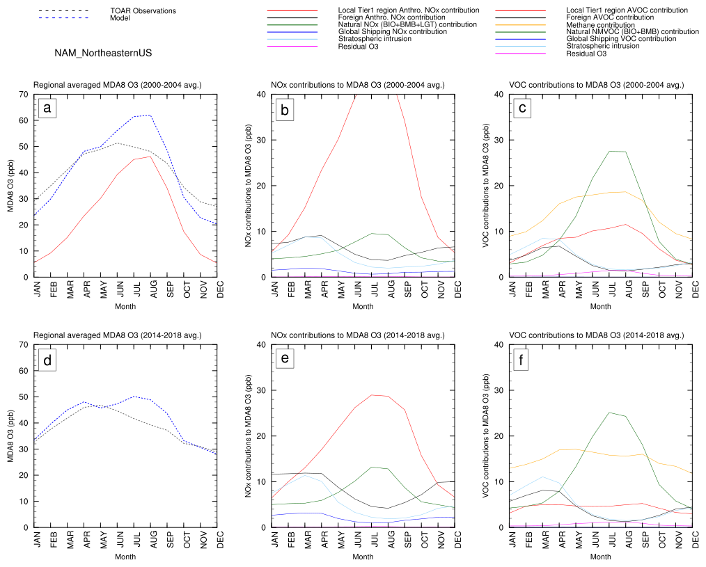
Figure 9 5 year average MDA8 O₃ seasonal cycles for NE US for 2000–2004 (a) and 2014–2018 (d) along with their NO_x (b, e) and VOC contributions (c, f).

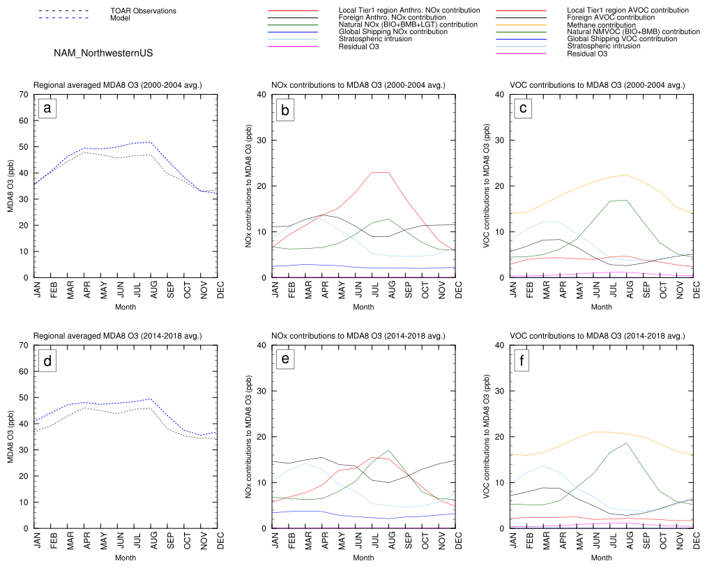
Figure 10 5 year average MDA8 O₃ seasonal cycles for NW US for 2000–2004 (a) and 2014–2018 (d) along with their NO_x (b, e) and VOC contributions (c, f).

The NE US (Fig. 9, Table 2) experienced more dramatic changes in its ozone seasonal cycle. The observed annual mean (y0) decreased from 40.4 ppb to 38.3 ppb. In contrast, the modeled y0 remained remarkably stable (fixed at 41.1 ppb), causing the model's initial slight positive bias to increase in the later period, particularly as modelled wintertime values increased more than observed ones. The most striking change is the substantial reduction in the amplitude of the annual cycle (A1), both in observations (from 11.8–6.7 ppb) and even more so in the model (from a highly overestimated 20.0–9.3 ppb). This signifies a major reduction in the summer peak. The phase of the annual peak (p1) also shifted significantly earlier in observations (from 5.4–5.0 months), indicating a pronounced shift of the seasonal maximum towards spring. The model also simulates an earlier peak (5.6–5.4 months), though the shift is less pronounced than observed, and the model still peaks later than observations in the recent period. The amplitude of the second harmonic (A2) increased in observations (1.3–2.2 ppb) but decreased in the model (3.9–2.3 ppb), suggesting evolving complexity in the seasonal shape that the model captures with mixed success.

These transformations are clearly linked to changes in NO_x and VOC contributions (Fig. 9b, c, e, and f). The dramatic decrease in A1 is primarily due to a large reduction in the summertime contribution from local anthropogenic NO_x (Figs. 9b vs. 10e). This local NO_x peak, which was very pronounced in 2000–2004 (contributing $\sim \mathrm{35}-\mathrm{45}\mathrm{ppb}$ in the model during summer), is significantly curtailed in 2014–2018 (contributing $\sim \mathrm{22}-\mathrm{28}\mathrm{ppb}$ in summer). While the model still appears to overestimate this summer local NO_x contribution in the later period (as suggested by a visual inspection of Fig. 9d as well as the still present overestimation of A1), the reduction is substantial. Concurrently, winter and spring ozone levels have increased (Fig. 9a vs. d). This is partly due to reduced wintertime titration by lower local NO_x, but also, as seen in the model (Fig. 9e), an increase in the foreign anthropogenic NO_x contribution during spring (8.3–10.8 ppb) and winter months (see Sect. 3.4 for a detailed analysis) as well as an increase in the stratospheric contributions (7.6–11.0 ppb; see Table 4). This increased foreign and stratospheric influx in spring, combined with the diminished summer photochemical peak, explains the observed shift in p1 towards an earlier (springtime) maximum.

From the VOC perspective (Fig. 9c vs. f), the summertime drop is driven by a large decrease in local AVOC contributions and a significant reduction in the contribution from natural VOCs. The latter is likely a consequence of the reduced local NO_x, making the natural VOCs less efficient at producing ozone, given that there is no correspondingly large decreasing trend in the BVOCs (Fig. 2). The wintertime increase in ozone is associated with an increased modeled contribution from methane, alongside the foreign AVOCs.

In the NW US (Fig. 10, Table 2), the evolution of the seasonal cycle from 2000–2004 to 2014–2018 is characterized by subtle but distinct changes (also see Fig. S2 and S3 for full envelopes). The observed annual mean ozone (y0) decreased slightly from 41.4–40.6 ppb, while the modeled y0 increased slightly (43.5–43.9 ppb), slightly increasing the positive bias noted earlier. The amplitude of the primary annual cycle (A1) shows a marked decrease in both observations (from 6.5 ppb to 5.2 ppb) and the model (from 9.0–5.3 ppb). This indicates a notable damping of the seasonal swing. Concurrently, the observed phase of the annual peak (p1) shifted slightly earlier, from 5.22–5.18 months, a trend also captured by the model (5.43–5.33 months) although these translate to a small shift of only a couple of days. The amplitude of the second harmonic (A2) also decreased, particularly in the observations (1.1–0.3 ppb), suggesting a smoother, less complex seasonal shape in the recent period.

These quantitative changes are driven by shifts in precursor contributions (Fig. 10b, c, e, and f). The most prominent change is the substantial reduction in the summertime peak of local anthropogenic NO_x contributions between the two periods (Fig. 10b vs. e) which directly contributes to the decreased A1. While this local contribution shrinks, the foreign anthropogenic NO_x contribution remains a significant and relatively stable component throughout the year, becoming proportionally more important, especially during spring; a finding consistent with a long line of previous studies (Berntsen et al., 1999; Jacob et al., 1999; Jaffe et al., 1999, 2003; Fiore et al., 2002; Parrish et al., 2014, 2022; Cooper et al., 2010; Simon et al., 2014; Parris and Ennis, 2019; Christiansen et al., 2022). The wintertime ozone levels show a slight increase (Fig. 10a vs. d), primarily linked to an increase in the modeled foreign NO_x contribution during these months in the later period. The springtime (March–May) ozone has seen increases in both foreign NO_x contributions (13.2–14.8 ppb) as well as stratospheric contributions (12.0–12.6 ppb; see Table 4 for a comparison across regions). Springtime mean stratospheric contribution is 12.6 ppb in the recent period (even higher in SW US at 14.3 ppb; Fig. S10; Table 4). Previous studies have reported modelled stratospheric contributions in North America during observationally-identified episodes with higher values (e.g., 20–40 ppb; Lin et al., 2012) as well as seasonal mean contributions (6–18 ppb; Mathur et al., 2022). Our seasonal mean values are lower likely because we do not sample the model output extensively from the mountainous region of western US, where stratospheric contributions are highest, due to lack of TOAR observations in those regions.

From a VOC perspective (Fig. 10c vs. f), the local AVOC contribution declined across all seasons, further contributing to the damping of the seasonal cycle (reduced A1). Methane remains a dominant VOC contributor, but its absolute contribution shows little change between the periods, suggesting its impact on seasonal amplitude is more modulated by NO_x availability than by its own concentration changes over this timeframe. The decrease in natural VOC contribution, particularly in summer, also plays a role in reducing A1. The overall effect is a flattening of the summer peak and a slight elevation of spring peak and winter trough, leading to the observed and modeled decrease in A1.

The quantitative analysis of seasonal cycle changes in NE US and NW US highlights the profound impact of declining local anthropogenic NO_x emissions. In both regions, this has led to a significant reduction in the amplitude of the annual ozone cycle (A1), particularly by lowering summer peaks. Wintertime ozone levels have generally increased, partly due to reduced local titration and partly due to increased contributions from remote sources like foreign anthropogenic NO_x and methane (these two effects are separately quantified in Sect. 3.4). The NE US exhibits a more pronounced shift, with a dramatic decrease in the summer peak and a clear move towards a spring-dominated seasonal maximum (earlier p1), a finding also reported by previous observation-based studies (Bloomer et al., 2010; Parrish et al., 2013; Cooper et al., 2014). This highlights the increasing relative importance of long-range transport in spring as local summer production wanes. The ongoing transition in the ozone seasonal cycle in the NE US, towards a springtime maximum, is expected to continue with future emissions changes, as discussed by Clifton et al. (2014). While the NW US also sees a damped cycle, its baseline remains more consistently influenced by foreign NO_x throughout the year. Our tagging technique, combined with Fourier analysis, allows for a quantitative attribution and evaluation of these changes. The increased share of foreign NO_x and methane in contributing to springtime ozone, which coincides with the agricultural growing season, highlights the impacts of intercontinental transported ozone on crop yields (Dingenen et al., 2009; Avnery et al., 2011) and ecosystem health, even as local emissions are successfully reduced.

3.3 Ozone in Europe

Here, we present the observed and model-derived results for different sub-regions in Europe: Western Europe, Southern Europe, C&E Europe, and SE Europe (see Fig. 3 for geographical extents). We first present trends in PSO along with their NO_x and VOC contributions, then show the 19 year average seasonal cycle of MDA8 O₃ and its source contributions, and finally present changes in the seasonal cycle between initial and the final five years. Europe has undergone significant reductions in NO_x emissions over the past decades (see Fig. 2), particularly in Western and Southern Europe (see Fig. 11). However, some countries in Central and Eastern Europe have not yet achieved the same level of reductions, suggesting potential variability in ozone trends across the continent. This raises important questions about how these uneven NO_x reductions might influence ozone formation dynamics in different sub-regions, which we explore in detail in this section using our tagged model results.

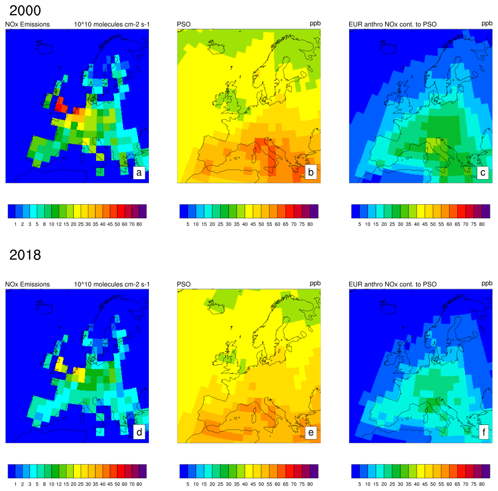
Figure 11 Spatial distribution of local anthropogenic NO_x emissions during peak season (a, d), PSO (b, e), and local anthropogenic NO_x contribution to PSO (c, f) for Europe during the initial (2000) and final year (2018). Here, emissions for each grid cell were calculated by averaging over a 6 month time window that matches the PSO window over the grid cell.

3.3.1 Peak season ozone in Europe: trends and source contributions

Figure 12 shows the observed and modelled PSO in different sub-regions of Europe along with the corresponding NO_x and VOC source contributions. We note that despite the large decline in European anthropogenic NO_x and NMVOC emissions (Fig. 2) over the two decades, the observed PSO values exceed the WHO long-term guidelines (31 ppb) in all regions. To understand the geographical backdrop of PSO changes, Fig. 11 presents a spatial map of local anthropogenic NO_x emissions (panels a, d), total PSO (panels b, e), and the modeled contribution of local anthropogenic NO_x to PSO (panels c, f) for the initial (2000) and final year (2018). In 2000 (Fig. 11a), prominent NO_x emission hotspots were evident (e.g., Benelux, Germany, Po Valley), parts of the UK, and major urban agglomerations across the continent. By 2018 (Fig. 11d), substantial emission reductions occurred, particularly in Western and Central Europe. However, this decline is not obviously reflected in the spatial patterns of total PSO (Fig. 11b and e), which generally decreased in the southern regions but not in northern regions, especially over areas with the largest emission cuts, as also seen in bias-corrected PSO maps by Becker et al. (2023). The direct contribution of local anthropogenic NO_x to PSO (Fig. 11c and f) mirrors these emission reductions more closely, with clear reductions from 2000–2018. This suggests the role of other contributions in offsetting the expected decline in PSO, especially in northern European regions.

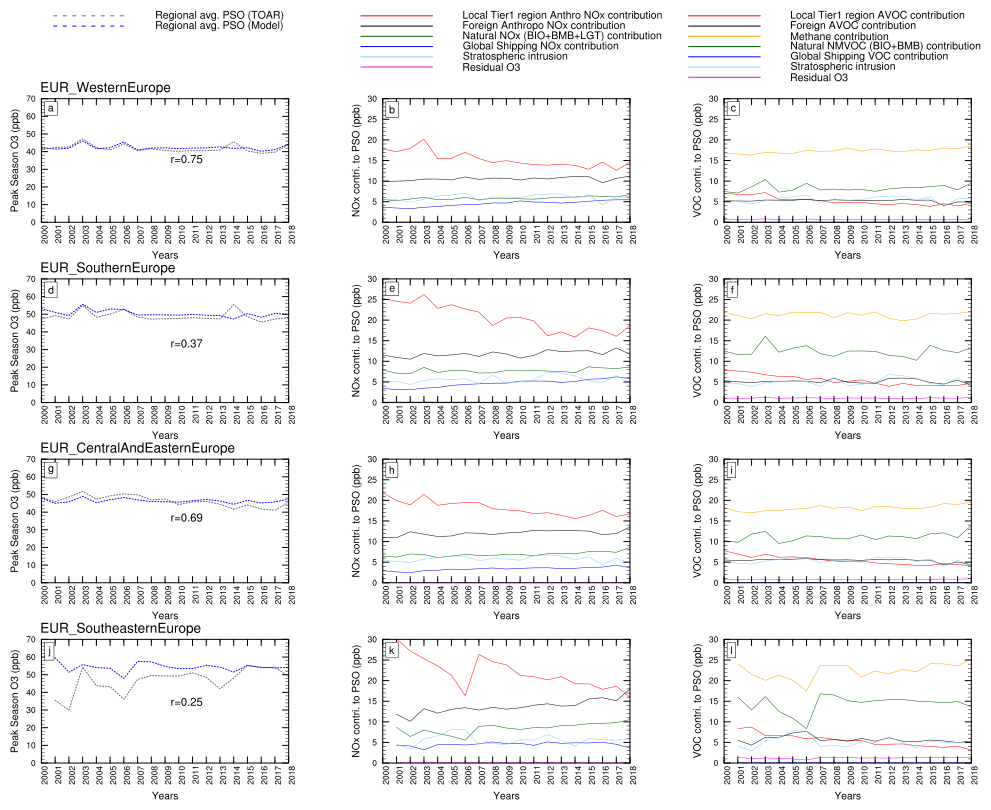
Figure 12 Time-series of observed and model-derived Peak Season Ozone for various receptor regions in Europe for 2000–2018 (left panels) and its source contributions in terms of NO_x sources (middle panels) and VOC sources (right panels). Model output was sampled from TOAR-valid grid cells only.

Table 3 Generalized Least Squares (GLS) linear trends in ppb/year along with their p-values (shown in parentheses) and 95 % confidence intervals (shown in square brackets) for observed and modelled Peak Season Ozone and its tagged source contributions for various receptor regions.

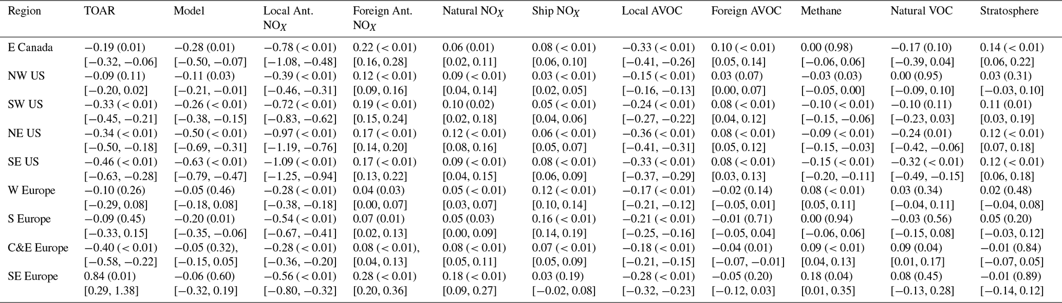
Table 4 Changes in the foreign anthropogenic NO_x contributions and stratospheric contributions to springtime (March–May) mean MDA8 O₃ in different receptor regions between the initial period (2000–2004) and recent period (2014–2018).

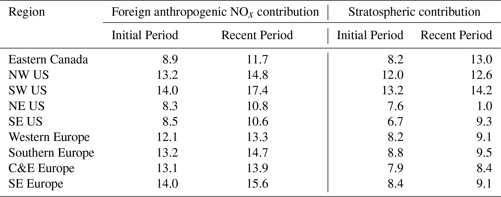
Observed PSO time series (Fig. 12, panels a, d, g, j) reveal diverse trends across Europe (see Table 3). Western Europe exhibits no significant long-term trend in observed PSO, despite a clear decline in local NO_x contributions. This region notably experienced high PSO during the 2003 and 2006 heatwaves (Vautard et al., 2013; Solberg et al., 2008; Struzewska and Kaminski, 2008), events which the model captures. Southern Europe shows a slight overall decline in observed PSO ($-\mathrm{0.09}\left(\mathrm{0.45}\right)[-\mathrm{0.33},\mathrm{0.15}]\mathrm{ppb}{\mathrm{yr}}^{-\mathrm{1}}$, Table 3), though with an uptick in the final years. C&E Europe displays a more pronounced decreasing trend in observed PSO ($-\mathrm{0.40}(<\mathrm{0.01}),[-\mathrm{0.58},-\mathrm{0.22}]\mathrm{ppb}{\mathrm{yr}}^{-\mathrm{1}}$). The model's performance in reproducing these trends varies: it captures the lack of trend in Western Europe and the declining trend in Southern Europe (albeit overestimating the declining trend; $-\mathrm{0.20}\left(\mathrm{0.01}\right)[-\mathrm{0.35},-\mathrm{0.06}]\mathrm{ppb}{\mathrm{yr}}^{-\mathrm{1}}$), but simulates a much weaker or even insignificant decline in C&E Europe than observed. The model generally also captures the interannual variability in PSO for Western Europe and C&E Europe successfully (r=0.75 and 0.69 respectively) and to a lesser extent in Southern Europe (r=0.37; Fig. 12). SE Europe presents a challenge for PSO trend interpretation due to lack of sufficient observational stations for most of the study period (see Fig. S14). Due to these sampling issues, we do not overinterpret the results for this region. Instead, we refer the reader to Lin et al. (2015) for a discussion on the dependence of the modelled ozone trends on the co-sampling with observations. Our results are in general agreement with the findings of Yan et al. (2018) who found insignificant trends for mean ozone but declining trends for the 95th %ile ozone in Europe during spring–summer.

The evolution of NO_x contributions to PSO (Fig. 12b, e, h, k; Table 3) is key to understanding European PSO trends. Local anthropogenic NO_x contributions (red lines) have declined significantly across all European regions. In Western Europe, this decline ($-\mathrm{0.28}(<\mathrm{0.01})[-\mathrm{0.38},-\mathrm{0.18}]\mathrm{ppb}{\mathrm{yr}}^{-\mathrm{1}}$) is offset by increases in other contributions, leading to a flat overall PSO trend. This quantitatively demonstrates that while local NO_x emission controls have reduced direct local ozone production, other contributions have compensated. In Southern Europe, the more stringent decline in local NO_x contribution (from ∼25 ppb in 2000 to ∼19 ppb in 2018) is the primary driver of the overall PSO decrease. C&E Europe also shows a substantial decline in local NO_x contribution ($-\mathrm{0.28}(<\mathrm{0.01}),[-\mathrm{0.36},-\mathrm{0.20}]\mathrm{ppb}{\mathrm{yr}}^{-\mathrm{1}}$). As for North America, we have also fitted exponential curves (based on Eq. 1) to the local anthropogenic NO_x contributions to PSO in European regions in order to facilitate the comparison of the e-folding time (τ) with observationally-derived values in published literature (see Fig. S16 and Table S10). We find a broad agreement with the observationally-derived values in that they are larger than those for North America ($\sim \mathrm{37}-\mathrm{63}\mathrm{yr}$ from the model and $\sim \mathrm{37}-\mathrm{44}\mathrm{yr}$ from observations), suggesting a relatively slower decline in local contributions in Europe.

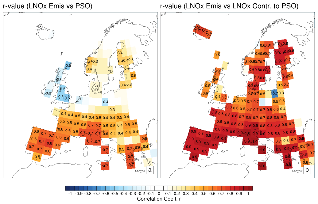
Figure 13 A spatial map showing correlation coefficient (r) between local anthropogenic NO_x versus PSO (a) and local anthropogenic NO_x versus local anthropogenic NO_x contribution to PSO (b) over the 19 years for Europe. For each year, and each gridcell, only peak season NO_x emissions were used per grid cell.

The relationship between local NO_x emissions and PSO is further illuminated by the correlation analysis in Fig. 13. The gridcell-level correlation between local anthropogenic NO_x emissions (averaged over the corresponding 6 month PSO window per year) and total PSO (Fig. 13a) is moderately positive over large parts of Central and Southern Europe (r $\sim \mathrm{0.4}-\mathrm{0.7}$), but weaker or even negative in parts of Western and Northern Europe. This indicates that while local emissions are a factor, total PSO in the northern belts of Europe is highly susceptible to other influences. In contrast, the correlation between local NO_x emissions and their direct contribution to PSO (Fig. 13b) is very high ($r>\mathrm{0.7}-\mathrm{0.9}$) across most of Europe. This confirms the model's source attribution capability and reinforces that reducing local NO_x directly curtails its specific ozone yield.

Foreign anthropogenic NO_x contributions have shown small increases across Europe (e.g., $\mathrm{0.04}\left(\mathrm{0.03}\right)[\mathrm{0.00},\mathrm{0.07}]\mathrm{ppb}{\mathrm{yr}}^{-\mathrm{1}}$ in Western Europe, $\mathrm{0.07}\left(\mathrm{0.01}\right)[\mathrm{0.02},\mathrm{0.13}]\mathrm{ppb}{\mathrm{yr}}^{-\mathrm{1}}$ in S Europe, $\mathrm{0.08}(<\mathrm{0.01}),[\mathrm{0.04},\mathrm{0.13}]\mathrm{ppb}{\mathrm{yr}}^{-\mathrm{1}}$ in C&E Europe), offsetting the benefits of local reductions (Fig. 12, panels b, e, h, k; Table 3). Global shipping NO_x contributions also show a consistent increasing trend across all European regions (e.g., $\mathrm{0.12}(<\mathrm{0.01})[\mathrm{0.10},\mathrm{0.14}]\mathrm{ppb}{\mathrm{yr}}^{-\mathrm{1}}$ in Western Europe, $\mathrm{0.16}(<\mathrm{0.01})[\mathrm{0.14},\mathrm{0.19}]\mathrm{ppb}{\mathrm{yr}}^{-\mathrm{1}}$ in Southern Europe), reflecting rising maritime emissions and their growing impact on coastal and inland air quality. Contributions from natural NO_x sources are also rising (see Table 3) despite the lack of a significant increase in natural NO_x emissions (Fig. 2) suggesting an increased ozone production efficiency by these emissions in a lower-NO_x environment, as also noted in North American regions. Stratospheric intrusion remains relatively small and a stable contributor to PSO without any significant trends (Table 3).

The VOC source contributions to PSO (Fig. 12, panels c, f, i, l; Table 3) reveal the significant role of methane and the impact of local emission changes. Methane is the largest VOC contributor to PSO across all European regions, typically around 15–20 ppb. Its contribution generally shows a slight increasing trend (e.g., $\mathrm{0.08}(<\mathrm{0.01})[\mathrm{0.05},\mathrm{0.11}]\mathrm{ppb}{\mathrm{yr}}^{-\mathrm{1}}$ in Western Europe), consistent with rising global methane concentrations, though this increase is modest compared to the overall PSO levels. Contributions from local AVOC have declined in all regions, mirroring reductions in their emissions and contributing to the overall PSO decrease where observed. For example, in Western Europe, local AVOCs declined by $-\mathrm{0.17}(<\mathrm{0.01})[-\mathrm{0.21},-\mathrm{0.12}]\mathrm{ppb}{\mathrm{yr}}^{-\mathrm{1}}$, and in Southern Europe by $-\mathrm{0.21}(<\mathrm{0.01})[-\mathrm{0.25},-\mathrm{0.16}]\mathrm{ppb}{\mathrm{yr}}^{-\mathrm{1}}$. This decline is consistent with reduced availability of both AVOCs and local NO_x for ozone formation. Natural VOCs (from biogenic and fire emissions) are the second most important VOC contributors after methane. Their absolute contribution varies, but like methane, their ozone production capacity is linked to NO_x availability. The interaction between local anthropogenic NO_x and natural VOCs is evident in all regions, where variability in the contribution from these two sources is highly similar. Foreign AVOCs, shipping VOCs, and stratospheric intrusion (VOC perspective) are smaller contributors, with foreign AVOCs and stratospheric components generally stable.

3.3.2 Ozone seasonal cycle in Europe: quantitative characterization and source contributions

Figure 14 shows the 19 year average seasonal cycle of MDA8 O₃ for different sub-regions of Europe along with its NO_x and VOC source contributions. The observed seasonal cycle is distinct in each receptor region: we see a major spring peak in Western Europe, a sustained spring-to-summer peak in Southern Europe and C&E Europe, and a major summer peak in SE Europe. The model reproduces the average seasonal cycles in these regions reasonably well, particularly in Western and Southern Europe. The model underestimates the MDA8 O₃ for C&E Europe in winter months and systematically overestimates the full seasonal cycle for SE Europe.

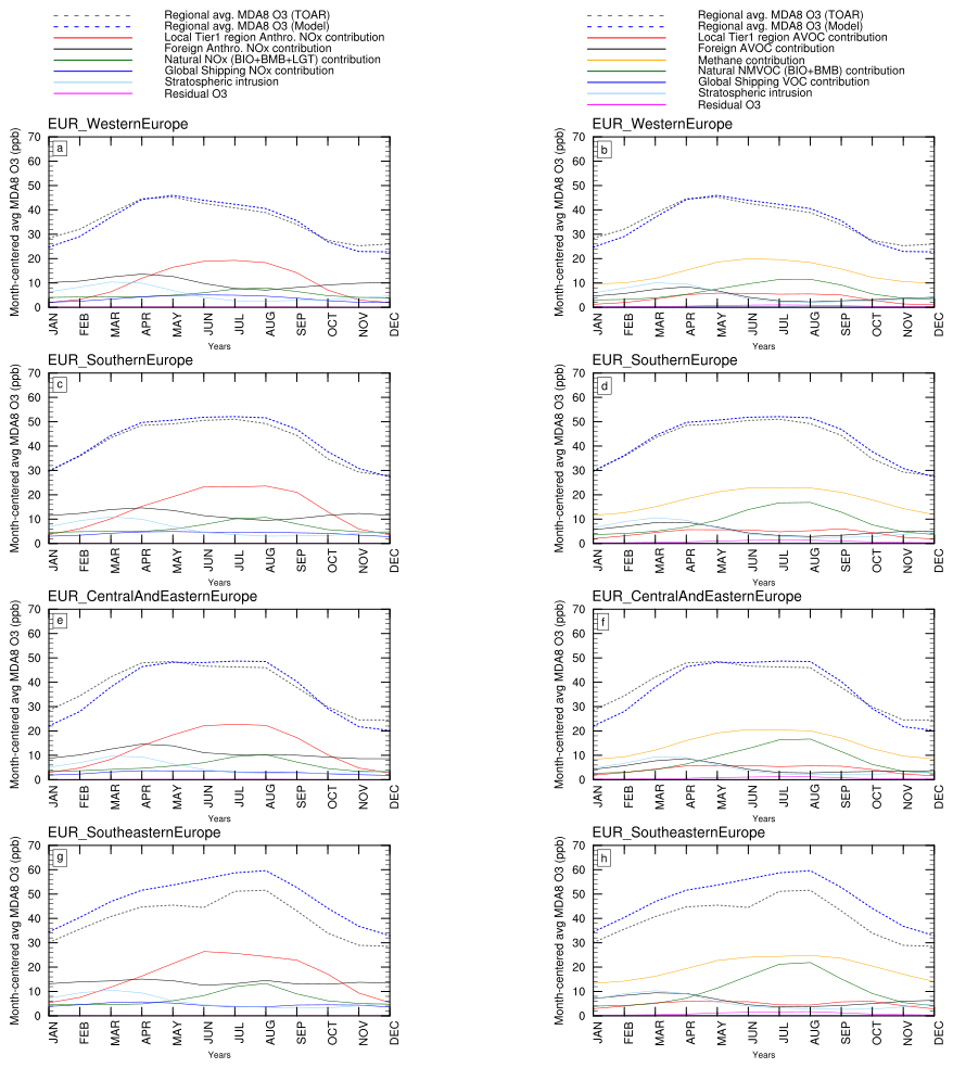
Figure 14 Month-centered average MDA8 O₃ over the 2000–2018 period for various receptor regions in Europe and its source contributions in terms of NO_x sources (left panels) and VOC sources (right panels). Model output was sampled from TOAR-valid grid cells only.

The 19 year (2000–2018) average seasonal cycle of MDA8 O₃ across European sub-regions was characterized using Fourier analysis, with parameters detailed in Table 2 and the cycles, along with source contributions, depicted in Fig. 14. Observed annual mean MDA8 O₃ (y0) across Europe is generally lower than in many North American regions, ranging from ∼35 ppb in Western Europe to ∼41 ppb in Southern Europe (Table 2). The model reproduces these annual means reasonably well for Western Europe (observed 35.4 ppb, modeled 34.7 ppb) and Southern Europe (observed 41.2 ppb, modeled 42.4 ppb). However, it underestimates y0 by ∼1.5 ppb in C&E Europe (observed 38.1 ppb, modeled 36.6 ppb) and significantly overestimates it by ∼7.5 ppb in SE Europe (observed 39.9 ppb, modeled 47.4 ppb). This large positive bias in y0 for SE Europe, also evident in the full seasonal cycle (Fig. 14g, h), may be influenced by uncertainties due to limited observational network affecting the gridded observational product in this sub-region (see Fig. S14).

The amplitude of the fundamental harmonic (A1), indicating the magnitude of seasonal variation, is substantial across Europe. Observed A1 ranges from 8.6 ppb in Western Europe to 11.6 ppb in Southern Europe. The model consistently overestimates A1 in all European regions, suggesting an overestimation of the summer photochemical peak. This overestimation is most pronounced in C&E Europe (modeled 15.2 ppb vs. observed 11.3 ppb) and Western Europe (modeled 11.1 ppb vs. observed 8.6 ppb). Overestimated A1 mirrors the findings for eastern North America and points towards an exaggerated summertime local ozone production, although this could only be conclusively determined by performing further perturbation experiments

The phase of the annual peak (p1) is relatively consistent across the regions, with observed values around 5.0–5.4 months, indicating a late spring to early summer maximum. SE Europe exhibits a slightly later observed peak (p1=5.6 months). The model generally captures this timing well, with modeled p1 values closely matching observations (e.g., Western Europe: obs. 5.0, mod. 5.2; Southern Europe: obs. 5.4, mod. 5.4). This agreement suggests the model correctly simulates the relative seasonal contributions of different processes driving the main ozone peak. For instance, the spring peak in Western Europe (Fig. 14a) is notably influenced by foreign NO_x and stratospheric contributions, while the broader spring-summer peak in Southern Europe and C&E Europe (Fig. 14c) reflects a strong summertime peak in local and natural NO_x contributions, alongside springtime transport influences.

The amplitude of the second harmonic (A2), representing semi-annual features, is generally smaller than A1 but non-negligible, with observed values between 1.8 ppb (C&E Europe) and 2.8 ppb (SE Europe). The model tends to reproduce A2 reasonably well for Western Europe and C&E Europe but overestimates it in Southern Europe (observed 1.8 ppb vs. modeled 2.6 ppb). A significant A2 can reflect the interplay between springtime transport-driven ozone enhancements and summer photochemical production. The phase of this second harmonic (p2) shows more variability and model-observation agreement is mixed.

The Fourier parameters are consistent with the source attribution patterns: for Western Europe (Fig. 14a and b), the distinct spring peak (captured by p1) is clearly driven by peaks in foreign NO_x and stratospheric contributions. The model's overestimation of A1 stems from a more pronounced modeled summertime contribution from local and natural NO_x than is suggested by the overall observed seasonal shape, which lacks a strong summer maximum. Methane is the dominant VOC contributor year-round. Southern and C&E Europe (Fig. 14c–f) exhibit a broader spring-to-summer high. Their larger A1 values reflect a strong summer peak in local anthropogenic NO_x and natural NO_x contributions, which the model captures but tends to exaggerate, leading to the overestimation of A1. Foreign NO_x contributes significantly to the spring shoulder and winter baseline. Methane and natural VOCs are key VOC contributors, especially during the warmer months. SE Europe (Fig. 14g and h) shows a clear summer maximum in observations and model (larger p1; delayed peak). Local and natural NO_x contributions drive the strong summer peak in the model.

The model effectively simulates the timing of the annual ozone peak (p1) across Europe. However, it consistently overestimates the amplitude of this annual cycle (A1), pointing to an overactive summer photochemistry in the model, a characteristic also noted for parts of North America. The annual mean ozone (y0) is well-reproduced for Western and Southern Europe but shows biases for Central and Eastern and particularly SE Europe. Wintertime ozone levels in all regions are sustained by significant foreign NO_x contributions (often >10 ppb), while summertime peaks are primarily driven by local anthropogenic and natural NO_x chemistry. Foreign AVOC contributions remain low ($<\mathrm{5}-\mathrm{7}\mathrm{ppb}$), suggesting limited interaction with European NO_x, implying that transported NO_x more significantly interacts with natural VOCs and globally present methane.

3.3.3 Changes in seasonal cycle of ozone in Europe: role of local vs. remote contributions

To understand the evolution of ozone seasonality in Europe, we compare the 5 year average MDA8 O₃ seasonal cycles from an initial period (2000–2004) with a recent period (2014–2018). Here, we present the results for Western Europe and Southern Europe, with detailed Fourier parameters in Table 2, and the corresponding seasonal cycles and source contributions in Figs. 15 and 16. Results for the remaining European sub-regions are included in the supplement (Figs. S9 and S10; Tables S8 and S9).

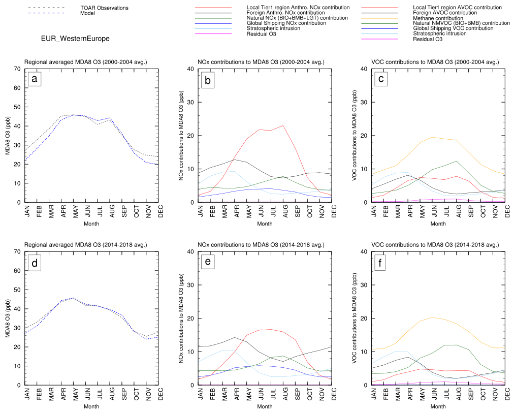
Figure 15 5 year average MDA8 O₃ seasonal cycles for Western Europe for 2000–2004 (a) and 2014–2018 (d) along with their NO_x (b, e) and VOC contributions (c, f).

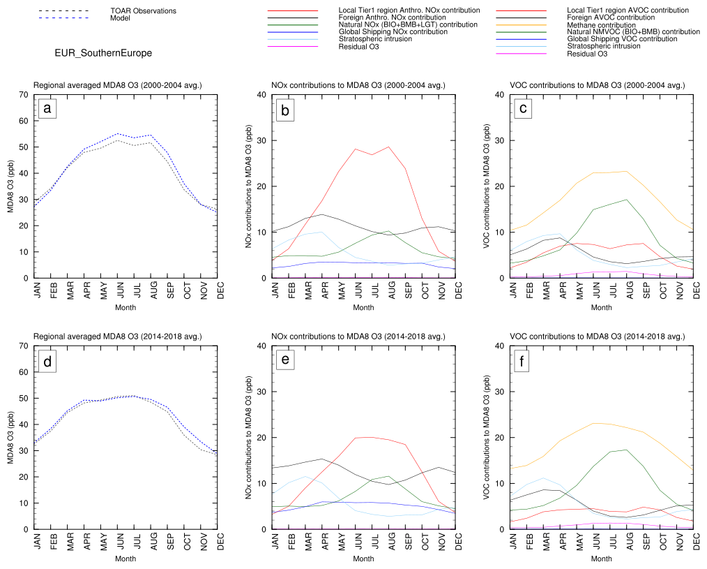
Figure 16 5 year average MDA8 O₃ seasonal cycles for Southern Europe for 2000–2004 (a) and 2014–2018 (d) along with their NO_x (b, e) and VOC contributions (c, f).

In Western Europe (Fig. 15, Table 2), the most notable change between 2000–2004 and 2014–2018 is a distinct flattening of the summer ozone peak alongside an increase in wintertime ozone levels. The observed annual mean MDA8 O₃ (y0) remained remarkably stable (35.8–35.8 ppb), a feature well-captured by the model (34.1–35.3 ppb). However, the amplitude of the primary annual cycle (A1), representing the summer–winter difference, decreased in both observations (from 10.1–8.0 ppb) and the model (from 13.2–9.5 ppb). This indicates a significant damping of the seasonal swing. The phase of the fundamental harmonic (p1) shifted slightly earlier in observations (5.2–5.1 months), as well as the model (5.3–5.2 months).

These changes are primarily driven by shifts in NO_x contributions (Fig. 15b vs. e). The summertime contribution from local anthropogenic NO_x decreased substantially between the two periods. This reduction in local summer production is the main cause of the lower summer peak and reduced A1. Conversely, wintertime ozone levels increased. This rise is linked to an increase in the foreign anthropogenic NO_x contribution during winter and spring months in the later period, coupled with reduced titration from lower local NO_x emissions (see Sect. 3.4 where these two effects are disentangled). It is noteworthy that the reduction in the local NO_x contribution during summer is larger than the overall decrease in total MDA8 O₃ during these months, because offsetting increases from other sources like shipping NO_x (which increased from ∼2 to ∼4 ppb in August) and a more efficient ozone production from remaining natural NO_x under lower overall NO_x conditions partly compensated for the local reductions. As noted previously, while Northern Hemispheric shipping NO_x emissions increased (Fig. 2e), the increased contribution from natural NO_x highlights its enhanced ozone-forming efficiency in a lower-NO_x environment. From a VOC perspective (Fig. 15c vs. f), the summertime decrease is associated with a reduction in local AVOC contributions. The wintertime ozone increase is supported by a larger share of methane contribution and, to a lesser extent, foreign AVOCs during winter in the recent period.

Southern Europe (Fig. 16, Table 2) also exhibits a notable evolution in its seasonal ozone cycle, characterized by a flattening of the seasonal cycle. The observed annual mean ozone (y0) slightly increased (from 40.83–41.81 ppb), a trend also seen in the model (42.0–42.8 ppb). The amplitude of the fundamental harmonic (A1) decreased significantly in observations (from 13.0–10.6 ppb) and even more so in the model (from 15.2–9.9 ppb), indicating a substantial reduction in the peak summer concentrations. The phase of the peak (p1) remained relatively stable, suggesting the timing of the summer maximum did not shift considerably.

The primary driver for the reduced summer peak and lower A1 is the marked decrease in the summertime contribution from local anthropogenic NO_x (Fig. 16b vs. e). While this local source remains the dominant contributor to the summer peak, its magnitude is considerably lower in 2014–2018 compared to 2000–2004. Similar to Western Europe, contributions from foreign anthropogenic NO_x have become relatively more important throughout the year, particularly sustaining spring and winter ozone levels. Natural NO_x and shipping NO_x contributions also show slight increases in summer in the later period, partially offsetting the local NO_x reductions.

Regarding VOC contributions (Fig. 16c vs. f), the summertime decrease in ozone is linked to reductions in both local AVOC and methane contributions during the peak season in the later period. Methane remains the largest VOC contributor overall, but its peak summer contribution has diminished. Wintertime ozone increases are associated with higher contributions from methane and foreign AVOCs, along with stratospheric intrusion.

3.4 Increasing foreign ozone in North America and Europe: increasing foreign NO_x emissions versus reduced local titration of background ozone

Previous sections highlighted an increasing trend in the contribution of foreign anthropogenic NO_x to ozone in various North American and European receptor regions, particularly during winter and spring (January–April). This observed increase in ozone attributed to foreign anthropogenic NO_x (hereafter, O3_FOREIGN) could stem from two primary mechanisms: (i) an actual increase in the intercontinental transport of ozone produced from foreign NO_x emissions, or (ii) an “unmasking” of transported ozone that was being previously titrated by local NO_x ($\mathrm{NO}+{\mathrm{O}}_{\mathrm{3}}\to {\mathrm{NO}}_{\mathrm{2}}+{\mathrm{O}}_{\mathrm{2}}$) but is not titrated anymore as local NO emissions have declined in these receptor regions. Disentangling these factors is crucial for making informed decisions on local as well as global emission reduction policies. For example, if the second mechanism is dominant, it would imply that with further local NO_x reductions we should expect more increases in winter-springtime ozone (which may potentially be a barrier to such policymaking). However, if the first mechanism is dominant, then further decreases in local NO_x will principally decrease local ozone while the transported component can be controlled through international policies.

To investigate this, we analyzed the combined contribution of O3_FOREIGN and the NO₂ formed from the titration of O3_FOREIGN (hereafter, NO2_FOREIGN). It is noteworthy that this NO2_FOREIGN, produced locally from titration of foreign ozone by locally-emitted NO_x, is separately tagged in our modelling system than the NO₂ directly flowing from foreign regions through reservoir species such as PAN and other organic nitrates (which we do not discuss here). The sum, Ox_FOREIGN (O3_FOREIGN + NO2_FOREIGN), represents the total reactive odd oxygen attributable to foreign anthropogenic NO_x sources. An increasing trend in Ox_FOREIGN would more strongly indicate an actual rise in transported reactive oxygen from foreign sources, whereas an increase in O3_FOREIGN with relatively stable Ox_FOREIGN might suggest a dominant role of reduced local titration.

Figure 17 presents the time series of winter-spring (January–April) mean O3_FOREIGN (blue shaded area) and the additional NO2_FOREIGN component (grey shaded area, making up the total Ox_FOREIGN indicated by the top of the grey area) for selected North American and European receptor regions over the 2000–2018 period. In both the NW US (Fig. 17a) and SW US (Fig. 17b), a clear increasing trend is evident not only in O3_FOREIGN but also in the total Ox_FOREIGN over the 2000–2018 period. For instance, in NW US, January–April mean O3_FOREIGN increased from approximately 10.3 ppb in 2000 to 13.3 ppb in 2018, while Ox_FOREIGN increased from approximately 10.8–13.6 ppb. Similarly, in SW US, O3_FOREIGN rose from around 10.6–13.7 ppb, and Ox_FOREIGN from 11.2–14.0 ppb. The NO2_FOREIGN component (grey area) is consistently small, typically ranging from 0.2–0.7 ppb during these cold, low-photolysis months. The key finding here is that the total Ox_FOREIGN shows a clear increasing trend. This robust increase in Ox_FOREIGN demonstrates that the rising influence of foreign NO_x on winter-spring ozone in western North America is substantially driven by an actual increase in the import of reactive odd oxygen from foreign sources, rather than solely by reduced local titration unmasking more foreign-produced background ozone. While reduced local titration plays a minor role (NO2_FOREIGN decreases over time), the fundamental increase in O3_FOREIGN is due to increasing foreign NO_x emissions. The Ox_FOREIGN peaks in 2013 when Northern Hemispheric NO_x emissions also peaked (see Fig. 2e). These results are consistent with findings of Elshorbany et al. (2024) and Lu et al. (2025) who report increasing ozone trends in Asia both in the troposphere and at the surface which stabilize around 2013. After 2013, we see a decline in both Ox_FOREIGN and O3_FOREIGN which is principally driven by a decline in foreign NO_x emissions (Crippa et al., 2023), which is primarily due to the implementation of China's Clean Air Programme (Zheng et al., 2018)

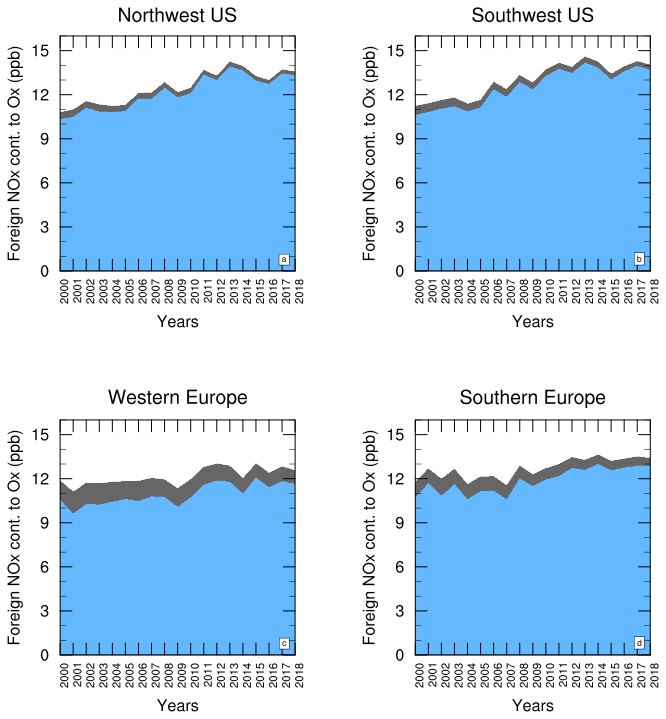
Figure 17 Time series of Foreign OX (O₃ + NO₂) contributions to wintertime and springtime (January–April) mean ozone in North American and European receptor regions. The blue shaded area denotes O₃ due to foreign anthropogenic NO_x and the grey shaded area denotes NO₂ originating from the titration of O₃ that is attributed to foreign anthropogenic NO_x.

Similar patterns are observed in Western Europe and Southern Europe (Fig. 17c and d, respectively). In Western Europe, winter-spring O3_FOREIGN increased from 10.6 ppb in 2000 to 11.6 ppb in 2018, with Ox_FOREIGN rising from 11.9 ppb to 12.6 ppb. Southern Europe saw O3_FOREIGN increase from around 10.7–12.9 ppb, and Ox_FOREIGN from 11.8–13.4 ppb. Again, the NO2_FOREIGN component remains a minor fraction of the total Ox_FOREIGN during these January–April periods and slightly decreases with time, reflecting reduced titration of O3_FOREIGN. The consistent increase in the total Ox_FOREIGN across these European regions, much like in North America, demonstrates an increasing influx of reactive odd oxygen attributed to foreign NO_x sources. This suggests that the observed rise in foreign ozone contributions during European winter–spring is not merely an artifact of changing local chemical environments (i.e., reduced titration) but reflects a more fundamental increase in the amount of pollution arriving from upwind, foreign sources.

4 Conclusion, limitations and future outlook

In this study we explain the long-term trends and the evolving shape of the seasonal cycle of surface ozone in North America and Europe (an issue raised by many previous observational studies) in terms of changing contributions from various NO_x and VOC sources, through the use of an ozone tagging system in a global chemical transport model. While both regions have experienced rapid reductions in locally-emitted ozone precursors in recent decades, we note that the Peak Season Ozone (PSO) in both regions exceeds the WHO long-term guidelines by wide margins for the entire study period.

Our model is generally in good agreement with ground observations from rural stations in the newly-developed TOAR-II database, allowing us to attribute the observed trends in terms of the changing contributions from local and foreign emission sources of NO_x and VOC. While AVOC emissions contribute a relatively small fraction of the total PSO, anthropogenic NO_x emissions have a much stronger influence. The decreasing trend in NO_x emissions in both North America and Europe leads to a lower fraction of the PSO attributable to these local NO_x emissions towards the recent years, however the total modelled decrease in PSO in both regions is partially offset by increasing contributions from natural NO_x, foreign anthropogenic NO_x, and international shipping.

While the increasing trend in ozone attributable to international shipping (despite potential overestimation of ozone produced from ships) is consistent with increasing emissions from this sector, the increasing trend in modelled contribution of natural NO_x emissions, especially during the summertime, suggests increasing ozone productivity of these emissions since there is no increasing trend in natural NO_x emissions in our model and a slight decreasing trend in Lightning NO_x emissions (Fig. 2a, c, e, and g). The decreases in local NO_x emissions in both regions lead to strong reductions in summertime ozone, but have a smaller effect in the springtime, when long-range transport of ozone produced from foreign anthropogenic NO_x emissions and stratosphere is more important (Table 4). All regions show a modest increasing trend in the foreign anthropogenic NO_x contribution to the PSOover the study period. Especially in the western sub-regions of Europe and North America, the foreign anthropogenic NO_x contribution to PSO has become comparable in magnitude to the local NO_x contribution. Foreign anthropogenic NO_x contribution to winter-springtime ozone has increased significantly and is primarily driven by increases in foreign NO_x emissions rather than reduced titration of foreign transported ozone, although the latter also plays a minor role. We have shown that local anthropogenic NO_x emissions still contribute significantly to PSO in both Europe and North America and its further reduction would not unmask a large amount of previously titrated ozone over regional scales in winter and spring. As an emission source which can be controlled with domestic policy interventions, future policy should continue to target these emissions.

Due to the nature of our ozone tagging system, we perform two separate source attributions, one for NO_x emissions, and another for VOC emissions. When attributing ozone to VOC emissions, we note the strong contribution of BVOC emissions to the summertime peak ozone, which is clearly linked with the strong contribution of local anthropogenic NO_x emissions to summertime ozone. The co-variability of these two sources is also apparent in the PSO time series for all regions and emphasizes the interaction of anthropogenic NO_x with BVOC in rural and background regions. This is an emerging finding made possible due to our dual-tagging approach; a relatively recent regional modelling study (Lupaşcu et al., 2022) focusing on two high ozone episodes in Germany that also utilized the TOAST1.0 system also noted the interaction of local anthropogenic NO_x and BVOC in driving ozone peaks.This finding highlights that, at least for rural and background regions, the interaction of anthropogenic NO_x with BVOC exceeds its interaction with AVOC which might be contained within the urban centres. It is noteworthy that BVOC emissions also either match or exceed AVOC emissions in North America and Europe during the peak season. In all of the sub-regions in our study except for the eastern parts of the United States, the contribution of methane to ozone is greater than that of BVOC. While global methane concentrations have risen from 1787–1875 ppb during our study period (an increase of about 5 %), this has only led to a modest increasing trend in methane contributions to PSO in Europe. In all regions of the US except NW US, the methane contribution to PSO has slightly decreased over this time. This is consistent with the large reductions in local NO_x emissions, leading to a lower efficiency of ozone production during methane oxidation over both regions.

The TOAST1.0 dual-tagging technique uniquely allows us to unveil many interesting results summarized above, which would not be possible to disentangle through perturbative approaches or other tagging approaches that tag a specific region with all its (NO_x + VOC) emissions or the geographic area of ozone production. It provides us with a parallel view of the composition of ozone trends in terms of NO_x and VOC precursors belonging to their original source locations, thereby facilitating a more targeted species-specific policy response. Many key results, for example: the separation of Foreign NO_x versus stratospheric contributions in explaining springtime ozone increase; separation of increased wintertime ozone to increased foreign NO_x versus reduced local titration; decreasing methane contribution to ozone in many regions despite increasing background methane; and in general the co-attribution of ozone to anthropogenic and biogenic emission sources under baseline conditions, would not be unveiled without the aid of our novel tagging system. Our innovative approach to model evaluation by breaking down the observed and modelled ozone seasonal cycles into a fundamental and secondary harmonic using Fourier transform and then comparing them against the seasonal cycles of tags (e.g., comparison of the fundamental harmonic against the local NO_x contribution to seasonal cycle) allows us to test the validity of such statistical decomposition techniques in different contexts and improve their theoretical interpretation; something which could not be achieved without tagged model simulations. Once sufficiently validated, such statistical decomposition could be applied more broadly, thereby unveiling new scientific insights from observations alone.

While this study has yielded an array of novel scientific results and policy-relevant insights, a number of limitations remain. First, our model spatial resolution (1.9°×2.5°), necessitated by the extra computational burden of tagged species and the long duration of the simulation period, is admittedly quite coarse and potentially introduces model biases. A recent study by Gao et al. (2025) has highlighted that the long-standing problem of overestimating surface ozone in the northern hemispheric mid-latitudes by global models can be addressed in large part by increasing the model resolution. Therefore, future modelling studies with tagging can be performed over short duration but high model resolution to assess the effect of model resolution on model bias and source contributions. Second, our source attribution, while capable of determining the contributions of different local and remote emission sources to the ozone under baseline conditions, is only of limited usefulness in predicting the response of ozone levels to any future emission reductions. For such an assessment, it is necessary to perform model sensitivity studies reflecting the actual policy interventions aimed at reducing ozone. Studies like ours can however identify the major contributing emission sources. Given the strong role of methane as an ozone precursor, targeted reductions of methane along with other AVOC can also be expected to contribute to the reductions in PSO needed to comply with the WHO long-term guideline value but such an assessment would require model perturbation studies wherein methane and AVOCs are reduced. Third, our approach does not attribute any changes in ozone to meteorological changes which might become increasingly important in a warming world. Instead, all changes in ozone are essentially attributed to precursor emissions. However, changing contributions from certain emission sources do not necessarily imply only changing emissions but could also be due to more/less efficient transport of foreign produced ozone due to meteorological changes.