Clear-sky and cloudy-sky differences in NO₂ concentrations over the United States: implications for satellite measurement applications

Satellite measurements of tropospheric trace gases are often only used when there are few clouds, which screens out 20 %–70 % of the data, depending on geographic region. Although clouds cause satellite data gaps, in situ surface measurements and model simulations can provide insight on NO₂ during cloudy conditions. Here, we intercompare surface observations, meteorological reanalysis (ERA5), satellite measurements (TROPOMI and TEMPO), and a model (WRF-Chem) during 2019 over the contiguous US to quantify how NO₂ concentrations differ under clear and cloudy skies. We find that in situ surface NO₂ measurements are, on average, +17 % larger on all days compared to clear-sky days and +36 % larger during cloudy days versus clear-sky days, with a wide distribution based on geographic region and roadway proximity: largest in the Northeast US and smallest in the Southwest US and near major roadways. WRF-Chem simulated surface NO₂ between cloudy and clear conditions is larger than the observed differences: +59 % on cloudy days vs. clear-sky days for the model. We additionally find modeled jNO₂ values are reasonable, suggesting this WRF-Chem NO₂ bias could be arising from overly rapid OH removal of NO₂ in sunlight, too slow NO_z regeneration of NO₂ in sunlight, or differing boundary layer depth biases under cloudy versus clear skies. Finally, using in situ NO₂ matched to provisional TEMPO data, we find the NO₂ differences between cloudy and clear conditions to be larger in the afternoon than morning. This study quantifies some of the biases in satellite measurements introduced by using only clear-sky data.

1 Introduction

Nitrogen dioxide (NO₂) is an air pollutant that adversely affects the human respiratory system (Health Effects Institute, 2022; Khreis et al., 2017) and can lead to premature mortality (Burnett et al., 2004; He et al., 2020). NO₂ is also an important precursor for ozone (O₃) and fine particulates (PM_2.5), which also have serious health impacts. NO_x (= NO + NO₂; most NO_x is emitted as NO which rapidly cycles to NO₂) is released into the atmosphere by biogenic microbial activity in soils, high-temperature lightning, wildfires, and thermal fossil fuel combustion; in urban areas, the majority of ambient NO₂ originates from the latter (Crippa et al., 2021). Although end-of-pipe controls (Busca et al., 1998; Koltsakis and Stamatelos, 1997) can reduce the amount of NO_x emitted from fossil-fuel engines and boilers, these technologies do not recover 100 % of the NO_x generation during combustion. As a consequence, NO₂ accumulates in our atmosphere and many urban areas have NO₂ concentrations that exceed the World Health Organization guideline of 5.3 ppb for an annual average (Anenberg et al., 2022).

Observing local air pollution is typically done by in situ surface monitors, which are spaced throughout a region with a higher density of monitors typically in areas of high population density and known pollution sources. In the United States, there are over 2200 in situ monitoring sites measuring some combination of O₃, PM_2.5, NO₂, volatile organic compounds (VOCs), and CO (U.S. EPA, 2023). While the US monitoring network is more comprehensive than most other countries (Martin et al., 2019), 79 % of US counties lack a single monitor and an additional 10 % of counties have only a single monitor, leaving only 11 % of US counties with more than 1 monitor (Sullivan and Krupnick, 2018). Although a robust and accurate ground-monitoring network is needed, the high operating cost of these instruments can be an important barrier (Kelly et al., 2017). Spatial gaps remain in-between the regulatory monitors, and sometimes these monitors are inadequate for understanding the true ambient air pollution exposure of most US residents, especially those that live and/or work several kilometers away from a regulatory monitor. Satellite data provide a way to fill in the gaps of the in situ monitoring network. Methodologies to obtain robust surface air pollutant measurement data from satellite instruments have improved dramatically in the past ten years (Bechle et al., 2015; Cao, 2023; Ghahremanloo et al., 2021, 2023; Larkin et al., 2023; Nawaz et al., 2025; Shetty et al., 2024; Sun et al., 2024).

NO₂ can be observed by remote sensing instruments due to its unique spectroscopic features (Vandaele et al., 1998). The Tropospheric Monitoring Instrument (TROPOMI) (Veefkind et al., 2012) has been measuring column densities of NO₂ pollution up to 7 × 3.5 km² before 6 August 2019 and up to 5.5 × 3.5 km² spatial resolution (van Geffen et al., 2024) since 6 August 2019. Because of TROPOMI's higher spatial resolution over predecessor instruments, such as the Ozone Monitoring Instrument (OMI) (24 × 13 km² at nadir) (Levelt et al., 2018), TROPOMI has ∼ 50 daily satellite pixel measurements within a typical city (∼ 1000 km²) during clear skies, while OMI may have only 1–3 daily measurements within the borders of each city. This increased measurement capacity within a city allows us to discern spatial variability undetectable by previous instruments (de Foy et al., 2009; Sun et al., 2018).

Level 2 satellite NO₂ measurements – which are retrieved from observed NO₂ spectra using geophysical and model-based assumptions – are of the tropospheric column. In many cases, NO₂ column measurements are strongly correlated with the spatial patterns of surface NO₂ concentrations (Acker et al., 2025; Harkey and Holloway, 2024; Kim et al., 2024) and surface NO_x emissions (Goldberg et al., 2024). For TROPOMI, studies have shown a strong correlation between tropospheric column measurements and collocated surface NO₂ for both the 13:30 average (r²=0.67) and the 24 h average (r²=0.68) (Goldberg et al., 2021; Kerr et al., 2023). However, there are rare instances in which NO_x emissions and NO₂ enhancements stay aloft and do not affect the surface; these are often situations associated with lightning NO_x (Nault et al., 2017), wildfire NO_x (Jin et al., 2021; Lin et al., 2024), and aircraft NO_x (Maruhashi et al., 2024). In these instances, it can be difficult to determine if the column NO₂ enhancements are also leading to surface NO₂ enhancements. These misinterpretations are more likely to occur over rural regions and/or individual days, as upper-tropospheric NO₂ enhancements near urban regions often dwarf NO₂ enhancements within the boundary layer especially over monthly or longer timescales (Goldberg et al., 2022).

Satellite measurements of trace gases are typically only used when there are few or no clouds; this is often referred to as the clear-sky bias of satellite data. In the US, this results in 20 %–70 % of the satellite data being filtered out depending on geographic region. The clear-sky bias affects NO₂ moreso than other trace gases (such as CO and CH₄) because NO₂ is very photochemically active in the presence of strong sunlight; its effective lifetime during summer daytime is 2–7 h (Liu et al., 2016) and conversely can be up to 30 h during winter daytime (Kenagy et al., 2018). The speed at which it transforms into other chemical species is determined by the irradiation, ambient temperature, and oxidative capacity (Laughner and Cohen, 2019; Shah et al., 2020). More specifically, strong irradiation creates the OH radical which can react with NO₂ to create HNO₃ – a major terminal sink of NO₂ – and also accelerates the photolysis of NO₂ into NO and O(³P) leading to an accumulation of O₃ in the presence of VOCs; without VOCs, NO₂ cycles more rapidly to NO. Warm temperatures increase biogenic VOC emissions and VOC can react with NO₂ directly to create organic nitrates (e.g., peroxyacetyl nitrates and alkyl nitrates) (Zare et al., 2018) which act as a temporary sink of NO₂. Another daytime terminal sink for NO₂ is dry deposition; while this removal mechanism is often secondary to photochemical loss in urban environments and is not directly affected by sunlight, it is indirectly affected as cloudy conditions are often associated with increased relative humidity and shallower boundary layer depths, both of which increase dry deposition fluxes. Therefore, increased NO₂ dry deposition fluxes in cloudy conditions could offset some of the decreased NO₂ photochemical loss rates. The net result is that NO₂ concentrations are typically larger during cloudy conditions (Geddes et al., 2012).

However, outside of the Geddes et al. (2012) study, little has been done to observationally quantify the bias of NO₂ being larger during cloudy conditions particularly because there are no column measurements to validate the satellite during cloudy conditions. With that said, there are surface in situ measurements during cloudy conditions that can give us an idea of how the clear-sky bias may affect the estimate of surface concentrations. In this project, we intercompare surface observations, meteorological reanalysis (ERA5), satellite measurements (TROPOMI and TEMPO), and a model (WRF-Chem) under clear and cloudy skies to better quantify the amount of surface and column bias of NO₂ concentrations that is being introduced when clouds are screened from the satellite data. Our analysis is focused on the United States during 2019 due the high density of in situ monitors and availability of high-resolution regional chemical transport models. The motivation of this project is to determine what the scientific community may be missing when excluding clouds from satellite-based NO₂ analyses.

2 Methods

2.1 EPA AQS Data

Hourly in situ NO₂ measurements were obtained from the pre-generated EPA Air Quality System (AQS) database: https://aqs.epa.gov/aqsweb/airdata/download_files.html (last access: 9 July 2025). These routine measurements are operated and maintained by various state and federal agencies. 91 % of the “NO₂” measurements in 2019 were acquired through a chemiluminescence technique which converts NO₂ and unintendedly some NO_z species – such as alkyl nitrates, peroxynitrates (PAN), and nitric acid (HNO₃) – to NO using a heated molybdenum converter; the NO is measured by quantifying the luminesce of NO when reacted in excess O₃ (Dickerson et al., 2019). Lamsal et al. (2008) suggested a correction factor for converting midday chemiluminescence NO${}_{\mathrm{2}}^{\ast }$ (= NO₂ + unintended NO_z) measurements to NO₂ using modelled information of PAN, alkyl nitrates, and HNO₃. In Eq. (1), we show the Lamsal et al. (2008) correction factor with a modification to exclude alkyl nitrates which are not explicitly included in our WRF-Chem simulation.

$$\begin{array}{}\text{(1)}& \begin{array}{rl}& {\left[{\mathrm{NO}}_{\mathrm{2}}\right]}^{\ast }=F_{\mathrm{int}}\times \left[{\mathrm{NO}}_{\mathrm{2}}\right]\\ & \text{where}{F}_{\mathrm{int}}={\displaystyle \frac{\left[{\mathrm{NO}}_{\mathrm{2}}\right]+\mathrm{0.95}\left[\mathrm{PAN}\right]+\mathrm{0.35}\left[{\mathrm{HNO}}_{\mathrm{3}}\right]}{\left[{\mathrm{NO}}_{\mathrm{2}}\right]}}\end{array}\end{array}$$

Typically, correction factors are in the range of ∼ 1.0 for fresh urban plumes and can be as large as ∼ 3.0 for rural areas during summer, with averages typically in the 1–1.5 range for moderate and very polluted regimes, and are important to use for model vs. monitor intercomparisons (Kuhn et al., 2024; Lamsal et al., 2008; Poraicu et al., 2023). Other methods to measure in situ NO₂ include Cavity Attenuated Phase Shift (Kebabian et al., 2008) and Laser Induced Fluorescence (Thornton et al., 2000), but these methods are less common (9 % of all NO₂ monitors in 2019).

Annual and seasonal averages at 13:30 local standard time (between 13:00–14:00) of the in situ data were considered valid and used if more than 75 % of the days of the year/season had valid data. There were 449 monitoring locations in 2019 in the US that achieved these criteria for an annual average, which equates to 1 monitor per ∼ 730 000 US residents. For the baseline analysis, we further remove data from the 75 monitoring locations (17 % of the locations) that are classified as “near-road” by the EPA, which means that they are installed within 20 m from major interstates since these in situ measurements are not representative of a ∼ 20 km² satellite pixel measurement; we include the “near-road” NO₂ monitoring data in sensitivity analyses. NO₂ measurements between cloudy and clear-sky days are intercompared using the normalized mean change (NMC) as described in Eq. (2), where $\overline{x}$ and $\overline{y}$ are means of the two datasets being analyzed.

$$\begin{array}{}\text{(2)}& \mathrm{NMC}\left(\mathit{\%}\right)=\mathrm{100}\times \left({\displaystyle \frac{\overline{y}-\overline{x}}{\overline{x}}}\right)\end{array}$$

2.2 Satellite NO₂ Instruments

NO₂ slant column densities are derived from radiance measurements in the 405–465 nm spectral window of the UV-VIS-NIR spectrometer (van Geffen et al., 2022; Nowlan et al., 2025). Satellite instruments observe NO₂ by comparing observed spectra with a reference spectrum to derive the amount of NO₂ in the atmosphere between the instrument and the surface; this technique is called differential optical absorption spectroscopy (DOAS) (Platt, 1994). Tropospheric vertical column density data, which represent the vertically integrated NO₂ concentrations between the surface and the tropopause, are then calculated by subtracting the stratospheric portion and then converting the tropospheric slant column to a vertical column using an air mass factor (AMF) (Boersma et al., 2011). The AMF is a unitless quantity used to convert the slant column into a vertical column and is a function of the satellite viewing angles, solar angles, the effective cloud radiance fraction and pressure, the vertical profile shape of NO₂ provided by a chemical transport model simulation, and the surface reflectivity (Lorente et al., 2017; Palmer et al., 2001).

2.2.1 TROPOMI

TROPOMI was launched by the European Space Agency (ESA) on 13 October 2017, and data from the instrument became available on 30 April 2018, after an approximately 6-month calibration period. The satellite follows a sun-synchronous, low-earth (825 km) orbit with an equator overpass time of approximately 13:30 local solar time. TROPOMI measures total column densities of several trace gases: NO₂, HCHO, O₃, CO, CH₄, among others. At nadir, pixel sizes are 3.5 × 7 km² (modified to 3.5 × 5.5 km² on 6 August 2019) with the edges having slightly larger pixels sizes (∼ 14 km wide) across a 2600 km swath, equating to 450 rows (van Geffen et al., 2020). For our analysis we use the TROPOMI NO₂ version 2.4 (V2.4) re-processed algorithm during 1 January 2019–31 December 2019. We also conducted a sensitivity study using the version 2.3.1 (V2.3.1) algorithm. The TROPOMI NO₂ V2.4 product has a documented median low bias of −34.8 % in moderately polluted locations (when NO₂ measurements are between $\mathrm{3}-\mathrm{14}\times {\mathrm{10}}^{\mathrm{15}}$ molec cm⁻²) when compared to a MAX-DOAS network (Lambert et al., 2023). Some of this low bias is due to the operational AMF which uses a 1° × 1° model to assume vertical shape profiles; when vertical shape profiles from a regional model are instead used, the bias decreases to between −1 % and −23 % (Nawaz et al., 2024; Judd et al., 2020; Tack et al., 2021). Prior work has demonstrated a strong correlation between TROPOMI NO₂ column measurements and NO₂ surface concentrations in urban areas (Demetillo et al., 2020; Dressel et al., 2022; Goldberg et al., 2021; Nawaz et al., 2025). For our baseline, we screened TROPOMI pixels for quality assurance flag values greater than 0.75, and conduct a sensitivity analysis of filtering only with a cloud radiative fraction filter of 0.5. The cloud radiative fraction is calculated from the O₂ A-band using the FRESCO-S algorithm. Due to differences in wavelength between the O₂ A-band and the NO₂ retrieval window, the cloud fraction retrieved in the O₂ A-band is not exactly representative for the cloud fraction in the NO₂ window, but it is similar.

The filtered data were re-gridded to a 0.01° × 0.01° resolution, to create a custom “Level-3” data product (Goldberg et al., 2021) during cloud-free and cloudy conditions. Single pixel TROPOMI tropospheric vertical column NO₂ uncertainties have been quantified to be between 25 %–50 % under clear skies and this uncertainty is dominated by uncertainty in the tropospheric air mass factor (Glissenaar et al., 2025; Liu et al., 2021; Rijsdijk et al., 2025); uncertainties of measurements with cloud fractions > 0.5 are larger. Oversampled NO₂ measurements over monthly and annual timeframes (10s–100s of measurements) have a smaller amount of uncertainty, approximately 10 %–20 % depending on location and season (Glissenaar et al., 2025).

2.2.2 TEMPO

TEMPO was launched by SpaceX on 7 April 2023 and is hosted on Maxar Intelsat 40e. Data from the instrument became available on 2 August 2023, after an approximately 4-month dry-out, cool-down, and calibration period. The satellite is in geostationary orbit centered over the United States with north-south coverage extending from Mexico City (∼ 17° N) to the Canadian Oil Sands (∼ 58° N) and east-west coverage from Puerto Rico to the Pacific coast. TEMPO operationally measures total column densities of NO₂, HCHO, and O₃ with additional products forthcoming. At nadir, pixel sizes are 4.75 × 2 km² with the North-east and North-west edges having slightly larger pixels sizes. The instrument observes the full east-west swath approximately once every hour.

For our analysis we use the TEMPO NO₂ version 3 algorithm during 2 August 2023–31 August 2024. The data was filtered to include pixels only where the effective cloud fractions are less than 0.15 and the main data quality flags are equal to 0. The filtered data was re-gridded to a 0.01° × 0.01° resolution, to create a custom “Level-3” data product (Goldberg et al., 2021) during cloud-free and cloudy conditions. Single pixel TEMPO tropospheric vertical column NO₂ uncertainties can be assumed to be similar to the uncertainty of TROPOMI measurements (Glissenaar et al., 2025), which are between 25 %–50 % under clear skies for individual pixels, and 10 %–20 % for oversampled averages; future work will better quantify the uncertainties of TEMPO NO₂ measurements.

2.3 ERA5 Re-analysis

We intercompare the cloud radiative fractions from TROPOMI to the ERA5 re-analysis (Hersbach et al., 2020) of total cloud fractions in the early afternoon (18:00 Z for Eastern Time, 19:00 Z for Central Time, 20:00 Z for Mountain Time, 21:00 Z for Pacific Time), which approximates the overpass time of TROPOMI over the contiguous United States. The ERA5 total cloud fraction is a unitless quantity representing how much of a grid cell is covered by a cloud (e.g., condensed water vapor) at any vertical level of the atmosphere and does not differentiate between the optical properties of those clouds. The ERA5 re-analysis data are reported at a 0.25° × 0.25° spatial resolution and the cloud fractions are interpolated, using bilinear interpolation, to the 0.01° × 0.01° oversampled TROPOMI NO₂ grid.

2.4 WRF-Chem

The Weather Research and Forecasting with Chemistry (WRF-Chem) model was run at 12 km × 12 km over the Continental US for all days of 2019: 1 January–31 December 2019 as described in He et al. (2024). For anthropogenic emissions, the Fuel-based Inventory of Vehicle Emissions (FIVE) was used to provide on-road and off-road mobile emissions, the Fuel-based Oil and Gas (FOG) inventory was used for emissions associated with oil and natural gas production, power plant emissions were provided by Continuous Emissions Monitoring Systems (CEMS), and all other anthropogenic emissions were obtained from the 2014 or 2017 National Emissions Inventory (NEI). Biogenic emissions were estimated using Biogenic Emissions Inventory System (BEIS) version 3.13. Gas-phase chemistry was from the RACM_ESRL_VCP scheme. Boundary conditions were provided from the Realtime Air Quality Modeling System (RAQMS, http://raqms-ops.ssec.wisc.edu/, last access: 12 November 2025) developed by the University of Wisconsin-Madison. The cloud fractions used in this project are from the total cloud fraction “CLDFRA” variable.

3 Results

3.1 CONUS Cloud Patterns

We first conduct an analysis of cloud patterns across the contiguous United States, and inter-compare clear-sky days estimated by TROPOMI, the ERA5 re-analysis, and the WRF-Chem model (Fig. 1). For TROPOMI, we define clear skies as the percentage of days with qa_value > 0.75, which almost exclusively filters based on cloud fractions < 0.5; cloud-free snow-covered scenes typically have a qa_value > 0.75 (Eskes et al., 2022). For ERA5 and WRF-Chem, we define clear skies as the percentage of days with the total cloud fractions < 0.5. ERA5 and WRF-Chem have similar clear-sky spatial patterns as TROPOMI but show systematically lower amounts of clear-skies by 8 %. The small systematic difference between TROPOMI and ERA5 when filtering for cloud fractions at 13:30 is likely driven by how optically thin cirrus-like clouds are handled; for TROPOMI these are being observed based on optical properties and therefore optically thin clouds are not assumed to be a cloud, whereas in weather models (ERA5 and WRF-Chem) these are being computed as vertical layers in the atmosphere with condensed water vapor. Overall, there is very strong agreement between the three datasets in the estimation of clouds giving us confidence that TROPOMI, ERA5, and WRF-Chem are all good estimators of daily clear-sky amounts.

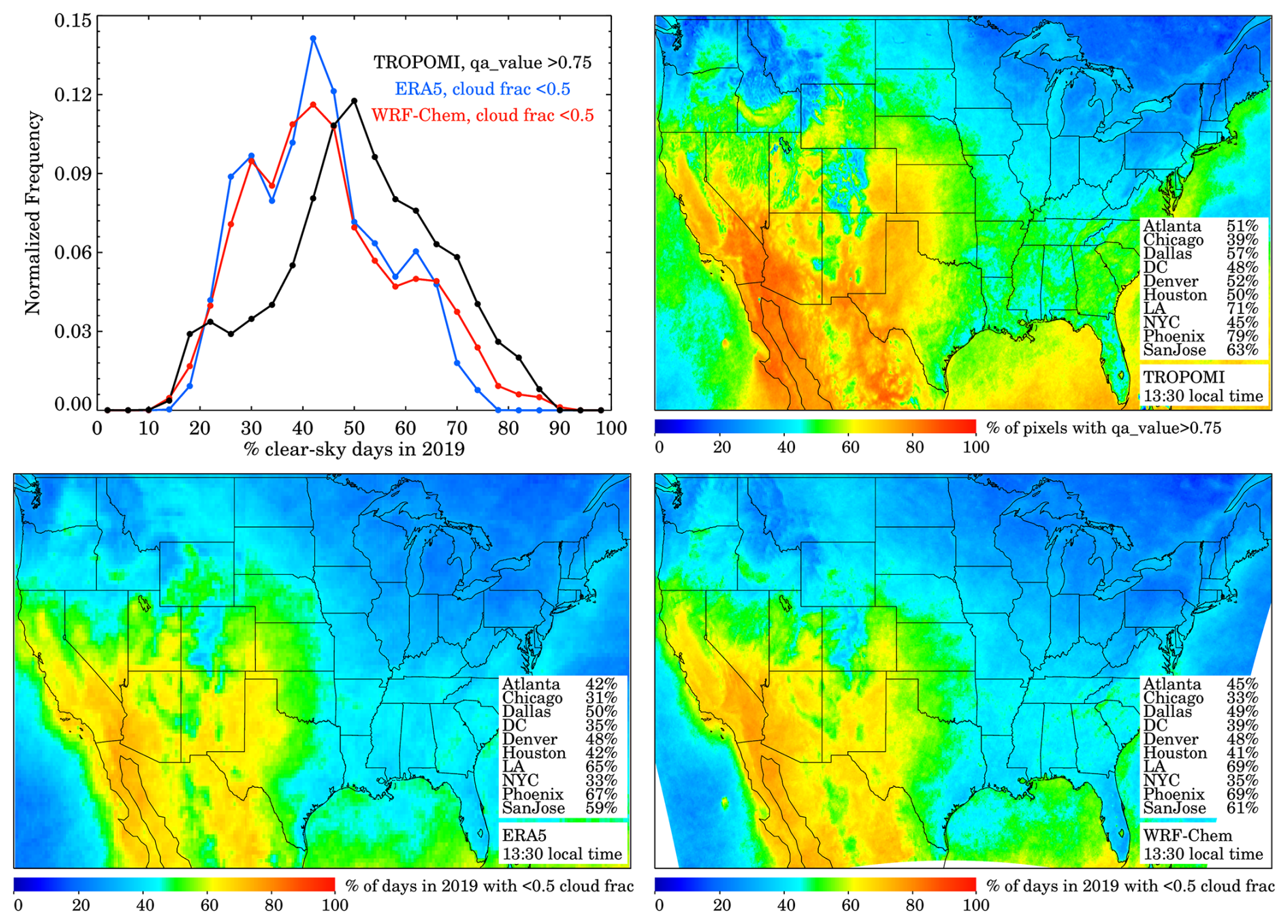
Figure 1 Percentage of clear-sky days over the contiguous US during 2019 from the TROPOMI NO₂ V2.4 product, ERA5 re-analysis, and WRF-Chem. (Top left) Normalized frequency diagram of the binned percentage of clear sky days for the three products. (Top right) Percentage of days in which the qa_value of the TROPOMI NO₂ V2.4 measurement was greater than 0.75. (Bottom left) Percentage of days in which the total cloud cover (tcc) from the ERA5 was less than 0.5. (Bottom right) Percentage of days in each grid cell in which the total cloud fraction from the WRF-Chem was less than 0.5.

For the remainder of this project, we define “clear sky” based on the TROPOMI NO₂ retrieval and use days with observations exceeding a qa_value of 0.75. According to TROPOMI – which is the only true observational dataset – the Southwest US has the most amount of clear-sky days per year (∼ 80 % of days at 13:30 local time), while the interior Northeast US and coastal Northwest has the fewest (∼ 30 % of days at 13:30 local time). The major US city with the most clear-sky days is Phoenix (79 % of days), while the major US city with the least clear-sky days is Seattle (29 % of days).

Annualized spatial cloud patterns are similar throughout the daylight hours with marginally more clear skies in the morning hours especially in the eastern US (Fig. S1 in the Supplement). Despite this, clouds are often transient, and there are opportunities to observe a clear sky measurement at a different hour of the day if the 13:30 observation is obstructed by clouds. In Fig. 2, we demonstrate that between 68 %–93 % of days have a clear sky measurement during any hour of the daytime as compared to the 33 %–69 % range at 13:30.

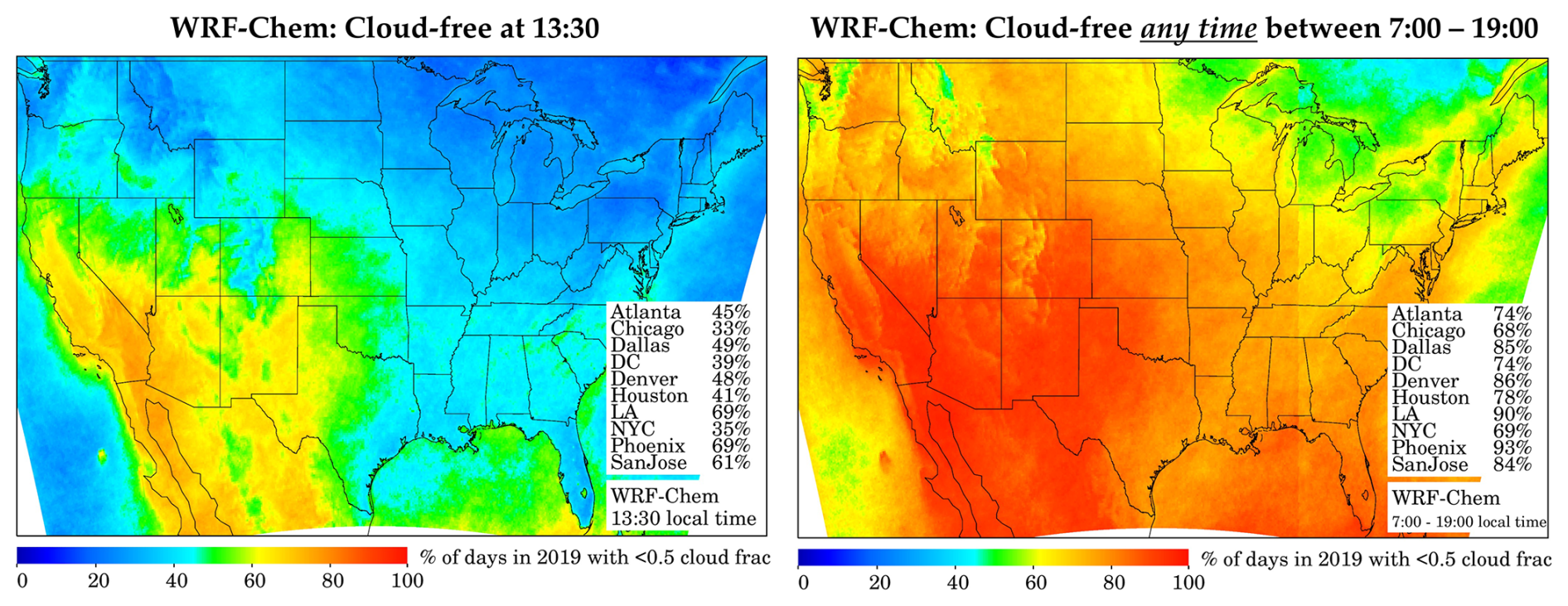
Figure 2 Percentage of days over the contiguous US during 2019 with cloud fractions less than 0.5 as simulated by WRF-Chem at various local times: (Left) 13:30, (Right) any time between 07:00–19:00.

3.2 Surface NO₂: Clouds vs. No Clouds

We then link whether TROPOMI is observing a clear sky or not (i.e., qa_value > 0.75) to the daily in situ ground-level NO₂ observations to determine how clouds are affecting surface NO₂ concentrations (hereafter referred to as surface NO₂). In Fig. 3, we show that surface NO₂ at 13:30 local time is +12.9 % larger (NMC = normalized mean change) [−3.8 % (10th percentile), +32.1 % (90th percentile)] on days with clouds at 13:30 compared to the annualized 13:30 average when all days of data are included. We also note the very strong correlation between the NO₂ on cloudy days and all days, which suggests that the presence of clouds drives a systematic change from the mean rather than a random change. We next show that the NO₂ during the average of all days is +17.2 % larger [−1.8 %, +38.7 %] than on days with only clear skies. We further show that surface NO₂ at 13:30 is +36.0 % larger [−6.1 %, +72.9 %] on days with clouds compared to days with clear skies.

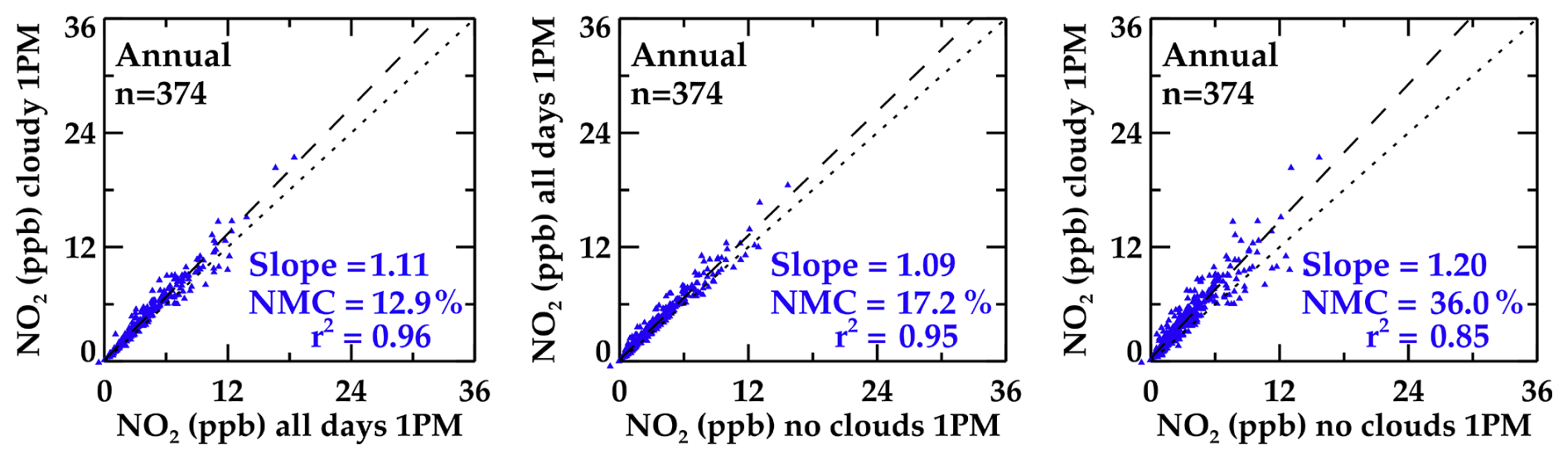
Figure 3 Scatterplots intercomparing annualized surface NO₂ from the EPA AQS at 13:30 local time during all days, cloudy days, and cloud free days. (Left) Annualized surface NO₂ during cloudy days compared to annualized surface NO₂ during all days. (Center) Annualized surface NO₂ during all days compared to annualized surface NO₂ during cloud free days. (Right) Annualized surface NO₂ during cloudy days compared to annualized surface NO₂ during no cloud. Each scatter point corresponds to each of the 374 measurement stations. A “cloudy” vs “no cloud” day is determined via the qa_value of 0.75 from the TROPOMI NO₂ V2.4 product.

The difference in surface NO₂ between cloudy and clear sky days can vary dramatically based on geographic region and proximity to a major roadway (Table 1). For the purposes of the sensitivity study, we focus on the cloudy versus cloud free days, while the directional changes of “cloudy versus all days” and “all days versus no clouds” values are similar (Tables S1 and S2 in the Supplement).

Table 1 Slope, r², Normalized Mean Change (NMC), and number of sites of the “cloudy vs. no clouds” bias by further filtering out AQS data using various additional sensitivity analyses. Tables S1 and S2 show the sensitivity analyses for the “cloudy vs. all days” bias, and “all days vs. no clouds” bias respectively.

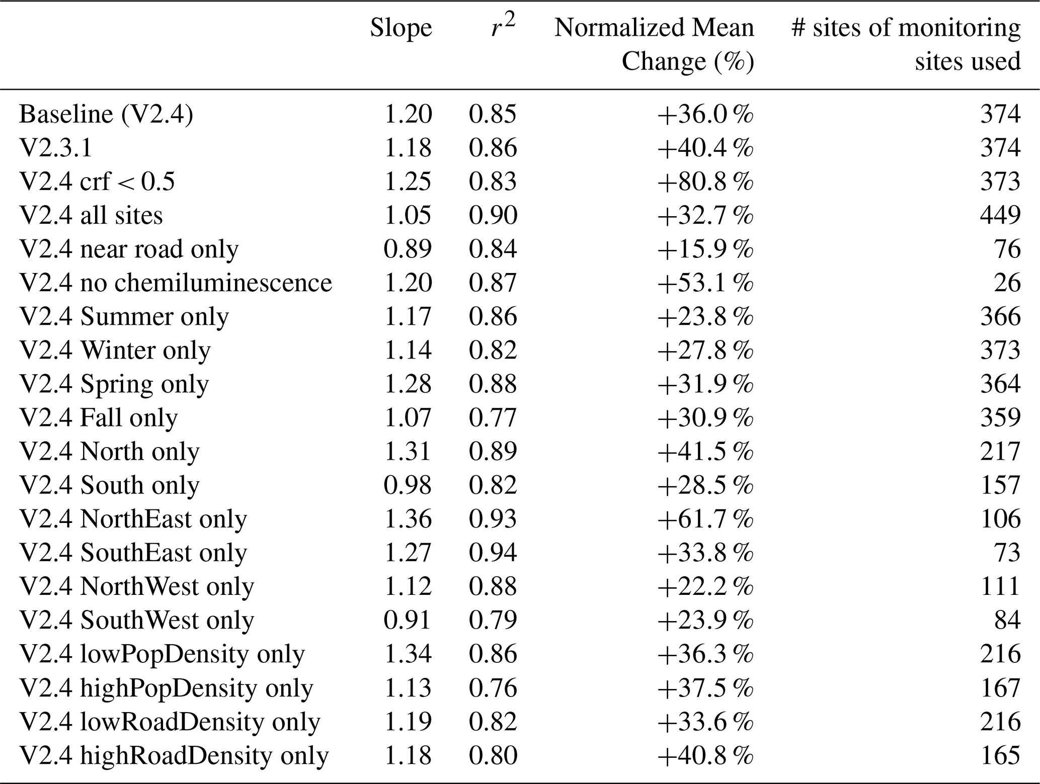
First, we find that NO₂ during cloudy days is larger in the northern US (+41.5 %) than the southern US (+28.5 %) and largest in the Northeast US (+61.7 %) (Fig. 4); for this analysis, 37° N is the dividing latitude between North and South, 100° W is the dividing longitude between East and West. Although the calculated cloudy versus no cloud change is independent of the number of days of clear-skies, areas of perpetually cloudy skies also have cooler temperatures, decreased photolysis, and shallower boundary layers which could cause much larger NO₂ on cloudy days. Interestingly, the Phoenix and Salt Lake City areas – two areas with large number of days with clear skies – also have a relatively large difference between cloudy and clear sky days demonstrating that the bias is independent of the number of days with clear skies. However, the annualized difference between cloudy and clear sky days in the Southwest US is modest (+4.8 %) (Table S1) because there are fewer individual days affected by clouds. Approximately 13 % of monitoring sites, mostly concentrated in the Los Angeles and San Diego areas, have lower NO₂ on cloudy days, and this may be driven by enhanced westerly winds on cloudy days bringing in cleaner marine air more than offsetting the photochemically driven larger NO₂ on cloudy days. Overall, while there are a few locations with lower NO₂ on cloudy days, 87 % of locations exhibit larger NO₂ on cloudy days and this is driven by the slower photochemistry on these days.

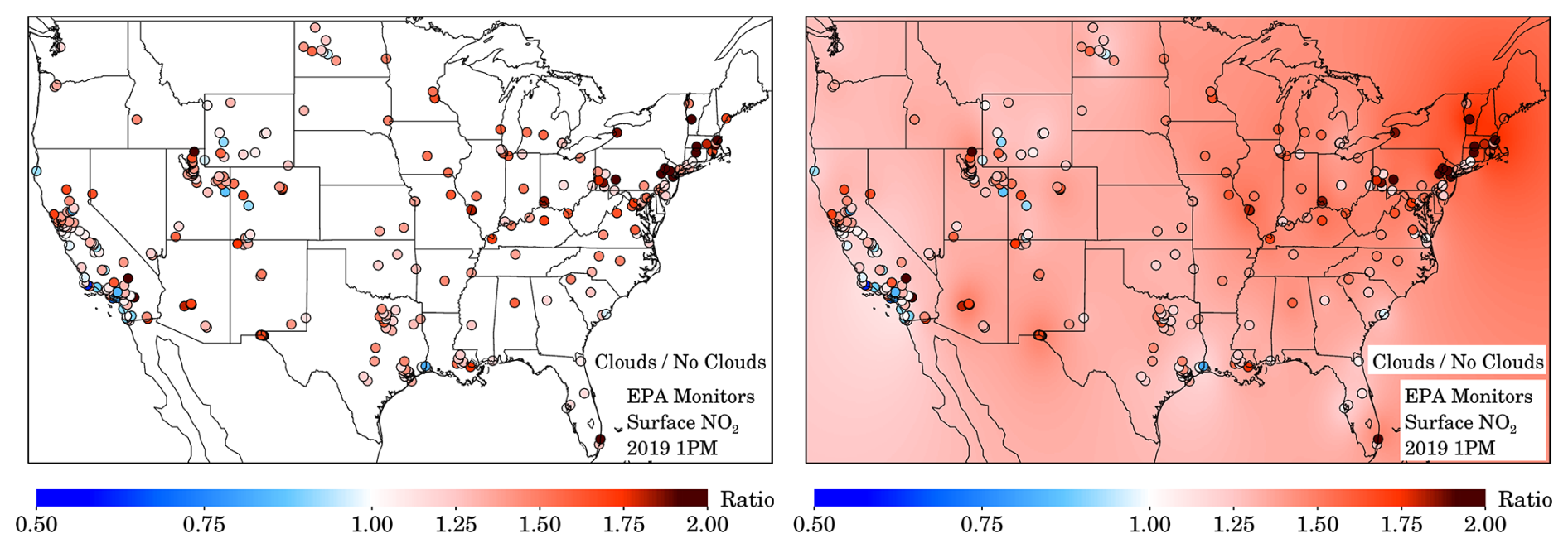
Figure 4 (Left) Ratio of the annualized surface NO₂ during cloudy and cloud free days at the EPA AQS sites not classified as “near-road”. (Right) Same image but with an inverse distance weighting underlaid to infer geographic distribution of the ratio.

Proximity to roadways and large sources of NO_x is another driver of whether a location will experience a small – but generally still positive – difference in NO₂ on cloudy and clear sky days. For areas in close proximity to roadways (i.e., the near-road sites) (n=76), the difference in NO₂ between cloudy and clear sky days is weaker: a smaller positive change (+15.9 %) and only 77 % of sites displaying a positive mean change, which is less than the difference at all other NO₂ monitoring locations (+36.0 %).

We find that seasonal effects on the differences in NO₂ between cloudy and clear days are modest. The NO₂ on cloudy days in the Spring is largest and marginally smaller in other seasons. Other factors that were not associated with strong changes to the differences in NO₂ between cloudy and clear days bias are: the version of the TROPOMI NO₂ algorithm, whether the site was using a chemiluminescence or Cavity Attenuated Phase Shift measurement technique, and population/roadway density within a 0.5° radius.

3.3 TROPOMI NO₂: Clouds versus No Clouds

We then compare TROPOMI NO₂ measurements under varying sky conditions to understand how the retrieved NO₂ columns differ under cloudy and clear-sky conditions, but not to answer how they actually differ. For this exercise, we filter the TROPOMI NO₂ data strictly based on cloud radiative fraction (crf). Although it is recommended for most applications to use data when the crf < 0.5, sometimes measurements are usable in the presence of optically thick clouds (i.e., crf > 0.5). In Fig. 5, we average TROPOMI NO₂ measurements below and above a crf = 0.5 threshold to gain an understanding of how TROPOMI column NO₂ measurements intercompare in the presence and lack of optically thick clouds. In the figure we show the tropospheric vertical columns on the top row, and tropospheric slant columns in the middle row, which have been interconverted using the tropospheric air mass factor shown on the bottom row. As discussed in Sect. 2.2.1, the tropospheric air mass factor can be a large source of uncertainty when calculating tropospheric vertical columns from slant columns (Glissenaar et al., 2025; Liu et al., 2021; Rijsdijk et al., 2025).

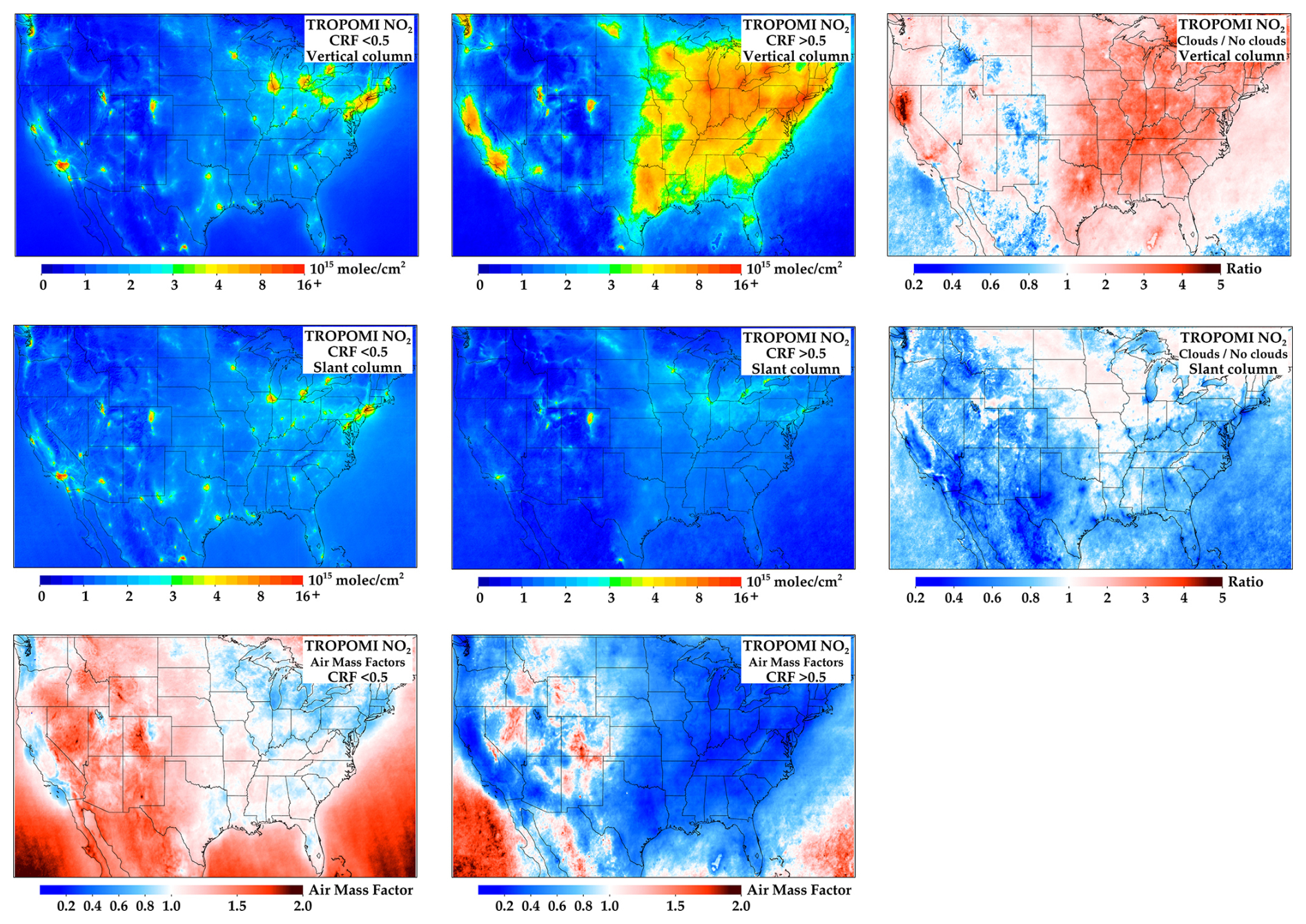
Figure 5 (Left column) Annual 2019 TROPOMI NO₂ filtered using only a cloud radiative fraction (crf) filter less than 0.5. (Center column) Annual 2019 TROPOMI NO₂ filtered using only a crf filter greater than 0.5. (Right column) Ratio between the two annual averages. (Top row) Vertical tropospheric column NO₂ data. (Center row) Slant tropospheric column NO₂ data. (Bottom row) Tropospheric air mass factors.

In Fig. 5, we demonstrate that the vertical column NO₂ spatial patterns in the presence of clouds are much different in magnitude than the slant column NO₂ whereas the vertical column NO₂ spatial patterns in the absence of clouds are similar to the slant column NO₂. This is primarily driven by the assumed scattering weights in the retrieval. During cloudy scenes, scattering and reflection by clouds reduce the satellite's sensitivity to near-surface NO₂, leading to smaller air mass factors as shown. Also, during measurements when the crf > 0.5, the uncertainty of the TROPOMI vertical column measurements rises, and this is driven by the difficulty in calculating the air mass factor in the presence of clouds; in addition to needing to know the vertical NO₂ profile for its calculation, we also need to know the pressure level and thickness of the clouds. Such errors can generate nonlinear responses. This analysis confirms that the assumed air mass factor is the driving factor causing the retrieved differences in the tropospheric vertical column NO₂ between clear and cloudy sky days, as the slant tropospheric column NO₂ is smaller during cloudy skies due to a lack of instrument sensitivity to the surface during cloudy conditions. Therefore, special care should be used when interpreting retrieved tropospheric satellite measurements in the presence of clouds.

Qualitatively, the ratio of the column NO₂ with and without clouds is spatially similar to the ratio from the AQS analysis – with the largest ratios occurring in the Northeast US and smallest ratios occurring in the Southwest US. However, quantitatively, the column ratio observed by TROPOMI is much larger in magnitude in the eastern US than the surface ratio observed at the AQS surface sites. It is difficult to determine whether the quantitative magnitude is correct because there are no ground-based instruments to accurately measure column NO₂ in the presence of clouds.

3.4 WRF-Chem NO₂: Clouds vs. No Clouds

We then compare the differences in NO₂ between cloudy and clear days observed by the EPA AQS surface network to the differences in NO₂ between cloudy and clear days of surface NO₂ simulated by WRF-Chem. The 13:30 local time differences in NO₂ between cloudy and clear days of surface NO₂ in WRF-Chem (+58.7 %) is substantially larger than from the AQS observations (+36.0 %) during collocations. This directional change is consistent among all geographic regions suggesting that NO₂ concentrations are too responsive to sunlight in WRF-Chem.

There could be several reasons for this discrepancy. First, 91 % of monitors in the EPA monitoring network measure using the chemiluminescence method, NO${}_{\mathrm{2}}^{\ast }$, which quantifies NO₂ in addition to some fraction of PAN, alkyl nitrates, and HNO₃. The latter is problematic because the NO₂+ OH → HNO₃ reaction is a photochemically-driven pathway for NO₂ during daytime and if HNO₃ is additionally being measured then this would appear to buffer photolytically driven changes. We further conducted a sensitivity test in WRF-Chem and found that the NMC is only +42.1 % down from +58.7 % when a chemiluminescence correction factor from Eq. (1) is used (Fig. 6c), indicating that some of the perceived differences between WRF-Chem and EPA monitors could be due to monitor interferences from PAN and HNO₃. Second, it is possible that radical concentrations (OH, HO₂, and/or RO₂) in WRF-Chem are fluctuating improperly in the presence of and lack of clouds (Duncan et al., 2024) causing NO₂ to either be removed too rapidly in the model or regenerated too slowly. Third, there might be insufficient photolysis of organic nitrates and/or particulate nitrates in the model which could buffer NO₂ photolysis-related changes; recent work has suggested that particulate nitrate can meaningfully photolyze back to NO₂ (Sarwar et al., 2024; Shah et al., 2024). Fourth, WRF-Chem may not simulate PBL depth properly and may have different biases during cloudy and clear sky conditions (Hegarty et al., 2018; Kuhn et al., 2024; Liu et al., 2023). For example, if the predicted PBL is too shallow during cloudy conditions, this could be a contributing factor to the simulated surface NO₂ bias. Errors in surface jNO₂ do not appear to be a primary driver of the cloudy versus clear sky disagreements as the jNO₂ values from WRF-Chem seem reasonable as compared to UV-B measurements from the NOAA Surface Radiation Budget (SURFRAD) monitoring network (Fig. S4) and is consistent with other work showing small biases in jNO₂ in WRF-Chem (Ryu et al., 2018). Follow-up work will address some of these shortcomings by adding particulate nitrate photolysis into the chemical mechanism and evaluating PBL depths during cloudy conditions using ceilometers.

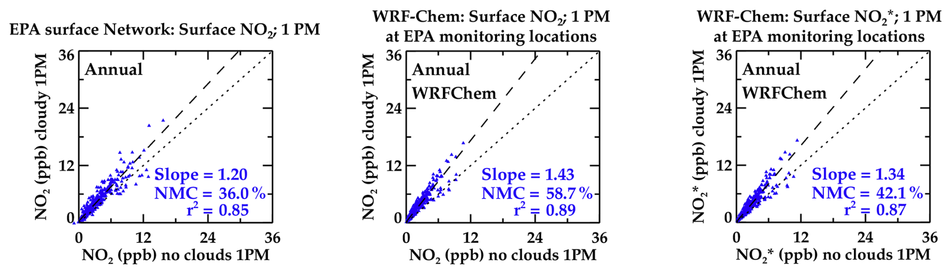
Figure 6 Scatterplots intercomparing annualized surface NO₂ at 13:30 local time during cloudy days vs. cloud free days. (Left) EPA AQS data which is a repeat of Fig. 3c. (Center) WRF-Chem collocated with the AQS monitoring sites, and using the WRF-Chem cloud filter in lieu of the TROPOMI cloud filter. (Right) WRF-Chem collocated with the AQS monitoring sites, comparing NO${}_{\mathrm{2}}^{*}$ instead of NO₂.

We can then use WRF-Chem as a transfer standard to suggest how column NO₂ may change in relation to the surface NO₂, and we find that the relative change in column NO₂ and surface NO₂ in response to clouds are very similar (Fig. 7). This makes intuitive sense because most NO₂ over the contiguous US is located within the boundary layer, and typically clouds (if they exist) are located at the top of the boundary layer. Any sunlight obstructed by clouds will also obstruct the NO₂ both at the surface and in the full boundary layer.

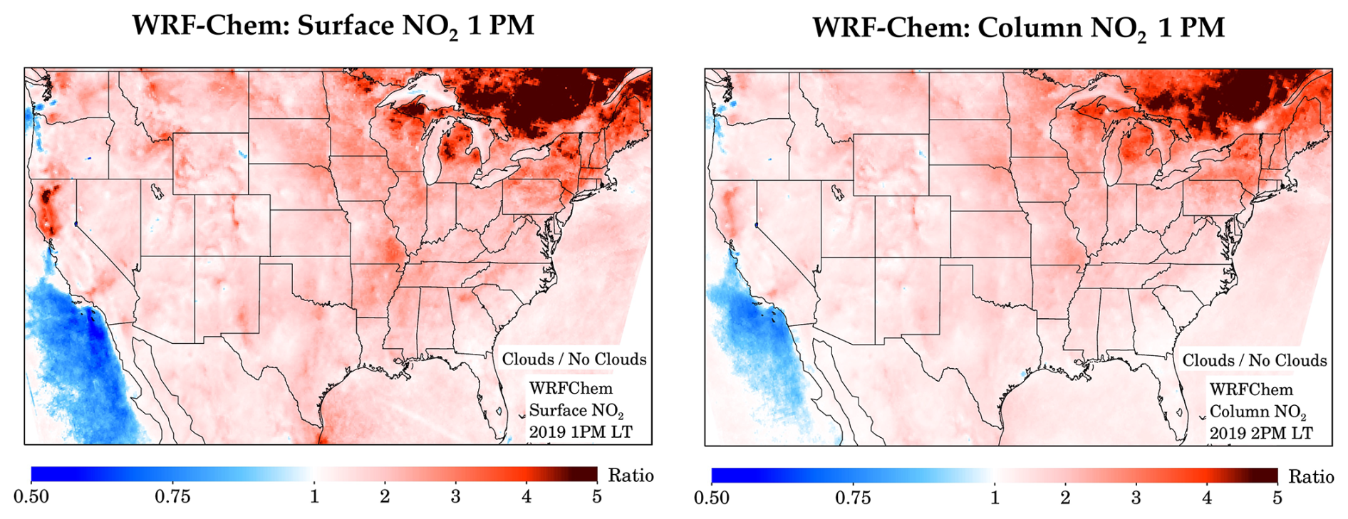
Figure 7 Ratio of the annualized surface NO₂ at 13:30 local time from WRF-Chem during cloudy and cloud free days. (Left) Surface NO₂ (Right) Tropospheric column NO₂.

3.5 Impacts of clouds on geostationary observations

Finally, we use provisional TEMPO NO₂ data, TROPOMI NO₂ data, and AQS NO₂ data from 2 August 2023 through 30 June 2024 to understand how the changes of NO₂ during clear and cloudy conditions may be altered at different hours of the day (Fig. 8). In this analysis, the threshold between high quality and lower quality data for both satellite products is a cloud radiative fraction = 0.15. Any TEMPO NO₂ or TROPOMI NO₂ measurement with crf  < 0.15 was assumed to be “clear sky”, while all other measurements are assumed to be cloudy. Hours with low solar zenith angles (before 08:00 and after 16:00) have been excluded from this analysis. We find that the difference in surface NO₂ between clear and cloudy days is small in the early morning hours and increases throughout the day.

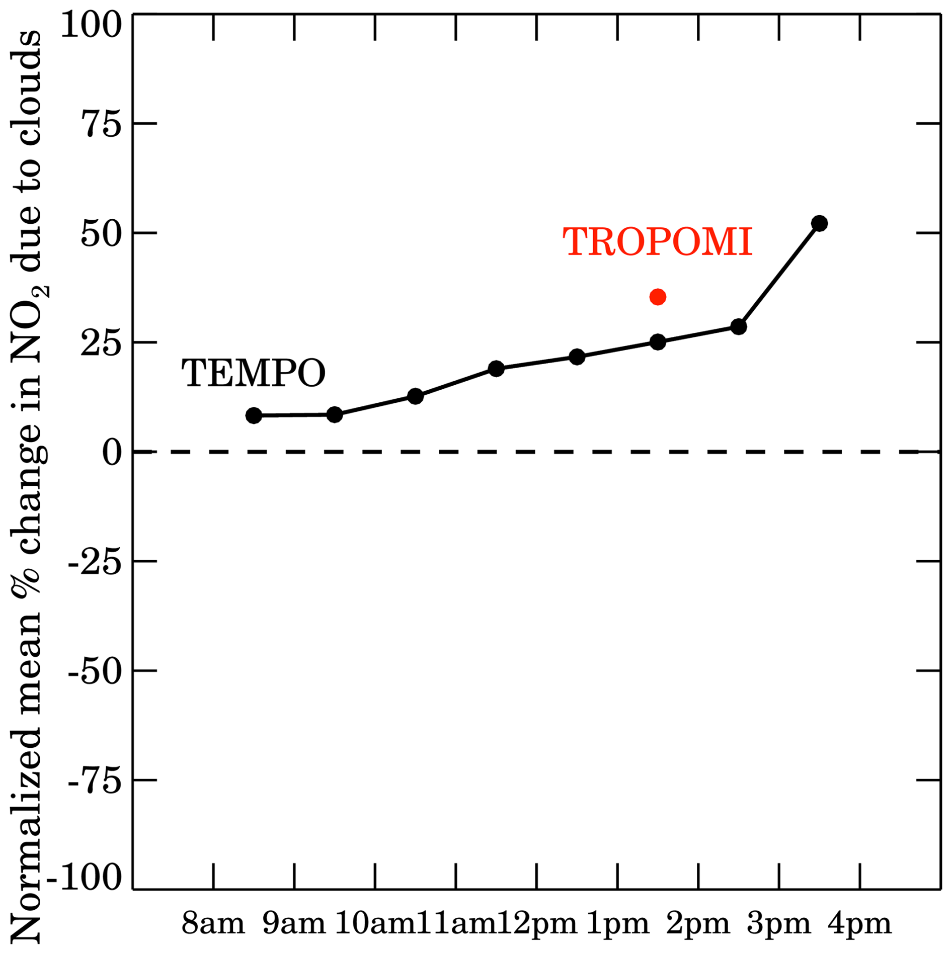
Figure 8 Normalized mean percentage change in the surface NO₂ during days with cloudy skies as opposed to days with clear skies. Red dot shows the mean percentage change using TROPOMI clouds as shown in Fig. 2c. Black line uses the same procedure for August 2023–June 2024 data and TEMPO cloud data.

Surface AQS NO₂ at 08:30 local time is +8.3 % larger on cloudy days than clear sky days, while at 15:30 it is +52.2 % larger. The calculated 13:30 difference in surface NO₂ between cloudy and clear sky days using TEMPO (+25.1 %) is similar to the analogous value from TROPOMI (+35.4 %). Differences between TEMPO and TROPOMI are expected because the cloud algorithms and instrument characteristics are different, even though the timeframe and cloud filter threshold used for this analysis are the same.

4 Discussion

In this project we quantify how NO₂ satellite data could be biased in estimating annualized surface NO₂ concentrations due to having high quality measurements only in the absence of clouds. We find that surface in situ NO₂ measurements are on average +17 % larger on all days compared to restricting to clear sky days and +36 % larger during cloudy days vs. clear sky days, with a wide distribution based on geographic region and proximity to roadway. Using the United States as a case study, we find the clear-sky bias to be largest in the Northeast US; conversely, the clear-sky bias is smallest in the Southwest US and near major roadways. In some areas of the urban Western US, Los Angeles and San Diego, we find that NO₂ is lower on cloudy days, but these instances are rare (13 % of monitoring sites) and are driven by unique transport patterns on cloudy days. Transport patterns are a significant driver of the regional clear vs. cloudy sky differences of surface NO₂ concentrations. Although the analysis was computed for both TROPOMI and TEMPO data, it should be re-emphasized that the cloud algorithms used by both instruments are different. However, the qualitative finding that surface NO₂ differences between cloudy and clear conditions tend to be larger in the afternoon than morning is consistent with a hypothesis that active photochemistry during periods of stronger afternoon sunlight would cause this change.

This work also highlights how NO₂ concentrations are different on days when satellite instruments are not acquiring a valid measurement. Our initial hypothesis of NO₂ being consistently larger on cloudy days was only partially proven true. In many cases, surface NO₂ concentrations and column NO₂ are larger, but this is not always the case. This project demonstrates the balancing act of the reduced NO₂+ OH sink and local climatological patterns (wind speed/direction, PBL depth, etc.) driving surface NO₂ during cloudy conditions. Although one of the original goals of this study was to better gap-fill satellite tropospheric vertical column NO₂ measurements in the presence of clouds, ultimately, we were not comfortable doing this yet. Reliance on a model as a transfer standard to convert surface concentrations into column concentrations exhibited too many biases under cloudy conditions. WRF-Chem model simulations of surface NO₂ suggest that the clear-sky bias in WRF-Chem is on average much larger than the observed clear-sky bias: +59 % on cloudy days vs. clear days for the model, and +36 % for the AQS data. We hypothesized that errors in OH chemistry, NO₂ recycling speeds, and PBL mixing depths could all be contributing to this high bias. Future work should target these three research topics. Future work could also use a machine-learning approach to account for some of these model biases.

Another consideration with the interpretation of satellite measurements is the impact of lightning NO_x, wildfire NO_x, and aircraft NO_x emissions, mostly staying aloft, which could be misinterpreted as surface NO₂ enhancements. While lightning NO_x and wildfire NO_x emissions are often screened out when applying a cloud filter because they occur in optically thick clouds/smoke, it is possible for the NO₂ to remain aloft for several days after the initial thunderstorm/fire and be observed during clear skies. An algorithm to detect and screen out downwind NO₂ attributed to upwind lightning NO_x and wildfire NO_x emissions could be especially helpful. At minimum, care should be taken during timeframes and regions where there are large pulses of these types of emissions, such as our findings during summer.

In some ways, the chosen year 2019 was an ideal year to conduct the analysis because it preceded the 2020 global pandemic and its nonlinear and lingering effects on air pollution. But in other ways, this year was less ideal because TROPOMI pixel sizes changed in August 2019 from 7 × 3.5 km² (∼ 25 km²) to 5.5 × 3.5 km² (∼ 19 km²). The fraction of clear-sky pixels likely increased by 1 %–2 % after August 2019 as smaller pixel sizes can better “see around” clouds (Krijger et al., 2007). This probably did not meaningfully affect our analysis but is nonetheless a caveat of using 2019 data.

These results have repercussions for many applied studies that use satellite data to estimate surface NO₂ concentrations or NO_x emissions. First, for studies that estimate surface concentrations, it is important to ingest surface NO₂ measurements during cloudy (and nighttime) conditions in some capacity in order to appropriately estimate 24 h concentrations; most studies already do this. If one were to use the clear-sky satellite data coupled with only a chemical transport model as a transfer standard to convert the column measurement into a pseudo-surface “measurement”, this would underestimate annualized NO₂ concentration in most places. Unfortunately, there are many global regions with few or no surface measurements, so this is an important consideration when estimating surface NO₂ in these regions. But even if one were to ingest surface NO₂ during cloudy conditions, the spatial patterns of surface NO₂ during cloudy conditions may be slightly different than implied by the clear-sky satellite data. For example, we find that NO₂ surface concentrations under cloudy conditions are much larger in the Northeast US than the Southwest US, and a cloud-free satellite map does not capture this.

Second, for nitrogen oxide emissions estimates it is often assumed that anthropogenic emission rates are similar under cloudy and clear-sky conditions, but this is likely not the case in reality. Although we show that surface NO₂ concentrations are typically smaller under clear-skies, it is likely that anthropogenic NO_x emissions are actually larger under regionwide clear-skies during summer and winter due to the moderating impact of clouds on surface temperature and subsequent impacts on heating-ventilation-air conditioning (HVAC) usage/emissions (Abel et al., 2017). If we were able to better independently estimate tropospheric vertical column NO₂ during cloudy conditions, perhaps this could be investigated in the future.

Lastly, as satellite-derived NO₂ applications increase over the coming years, it is important to document its successes and shortcomings. We see this project as a first-step towards better accounting for the clear-sky bias of satellite NO₂ data. While future NO₂ applications may use geostationary data, such as TEMPO, which may suffer from a similar bias depending on the hour of the day, an advantage of geostationary satellite data is the ability to use multiple measurements per day before and just after the clouds. It might be possible to isolate a two-hour window (one with a cloud and one without) to get a better handle on the instantaneous versus long-term role of clouds affecting NO₂ concentrations.

This work also highlights the critical role that chemical transport models can play in satellite NO₂ applications. Errors in the model assumptions can hamstring many NO₂ applications. For example, using a model to infer NO₂ during cloudy conditions in the lack of clear-sky satellite data would yield significant errors. Therefore, future work should concurrently focus on acquiring and using sub-orbital measurements to diagnose errors related in simulating NO₂ in chemical transport models, so that they can be used as more robust transfer standards.