All-sky direct aerosol radiative effects estimated from integrated A-Train satellite measurements

The improvement of satellite-derived calculations of direct aerosol radiative effects (DARE) is essential for reducing the uncertainty in the impact of aerosol on solar radiation. We develop a framework to compute DARE at the top of the Earth's atmosphere, in the shortwave part of the electromagnetic spectrum, and in all-sky conditions along the track of the A-Train constellation of satellites. We use combined state-of-the-art aerosol and cloud properties from the Cloud-Aerosol Lidar with Orthogonal Polarization (CALIOP) and the Moderate Resolution Imaging Spectroradiometer (MODIS) satellite sensors. We also use a global reanalysis from the Modern-Era Retrospective Analysis for Research and Applications version 2 (MERRA-2) to provide vertical distribution of aerosol properties and atmospheric conditions. Diurnal mean satellite DARE values range from −25 W m⁻² (cooling) to 40 W m⁻² (warming) over the southeast Atlantic during 3 days from the NASA ObseRvations of Aerosols above CLouds and their intEractionS (ORACLES) aircraft campaign. These 3 days indicate agreement between our satellite-calculated DARE and co-located airborne Solar Spectral Flux Radiometer (SSFR) measurements. This paper constitutes the first step before applying our algorithm to more years of combined satellite and model data over more regions of the world. The goal is to ultimately assess the order of importance of atmospheric parameters in the calculation of DARE for specific aerosol and cloud regimes. This will inform future missions about where, when, and how accurately the retrievals should be performed to reduce all-sky DARE uncertainties.

1 Introduction

Small suspended individual particles (aerosols) can scatter, reflect, and/or absorb incoming sunlight (also called direct aerosol–radiation interactions) and influence cloud properties (also called aerosol–cloud interactions or indirect aerosol–radiation interactions), both of which perturb the radiation balance of the Earth's atmosphere. The impact of aerosols on solar radiation plays a key role in the Earth's climate as they offset roughly one-third of the warming from anthropogenic greenhouse gases (Li et al., 2022). The aerosol radiative effect is the immediate impact of aerosols on the radiation budget, while the aerosol radiative forcing is the change in that impact compared to pre-industrial times. Reducing uncertainties in the total aerosol radiative forcing contributes to reducing uncertainty in quantifying present-day climate change (Forster et al., 2021). Although uncertainties in aerosol–cloud interactions dominate the total aerosol radiative forcing (given a global anthropogenic aerosol radiative forcing of $-\mathrm{1.0}\pm \mathrm{0.7}$ W m⁻²), uncertainties due to aerosol–radiation interactions are still of the order of 100 % (given a global anthropogenic radiative forcing of $-\mathrm{0.3}\pm \mathrm{0.3}$ W m⁻²) (Forster et al., 2021). These uncertainties represent model diversity and are generally considered a lower bound on uncertainty (e.g., Li et al., 2022). To illustrate, Myhre et al. (2013) conducted aerosol comparisons between observations and models and reported a large inter-model spread in the radiative forcing due to aerosol–radiation interactions (RFari) of the aerosol species. For example, a range from 0.05 to 0.37 W m⁻² in RFari exists from black carbon (BC; the dominant light-absorbing biomass burning (BB) smoke aerosol component across all visible wavelengths), with a standard deviation of 0.07 W m⁻² compared to a mean RFari of 0.18 W m⁻² of BC (i.e., a 40 % relative standard deviation). Our study focuses on the instantaneous or diurnally averaged direct aerosol radiative effect (i.e., without consideration of pre-industrial times) in the shortwave (SW) part of the electromagnetic spectrum (i.e., four broadband channels between 345 and 1242 nm, to be exact), at the top of the atmosphere (TOA), in all-sky conditions (i.e., in cloud-free and cloudy-sky conditions) without distinguishing between aerosols from humanmade (anthropogenic) or natural sources.

The instantaneous TOA SW direct aerosol radiative effects (DARE) – referred to as DARE in W m⁻² – quantify the difference in the net radiative flux at TOA, F^net, due to perturbations in the loading of aerosol in the atmosphere, which can be expressed by the following equation:

$$\begin{array}{}\text{(1)}& \begin{array}{rl}{\mathrm{DARE}}^{\mathrm{TOA}}& =F_{\mathrm{aerosol}\mathrm{present}}^{\mathrm{net}}-F_{\mathrm{no}\mathrm{aerosol}\mathrm{present}}^{\mathrm{net}}\\ & =\left(F_{\mathrm{aerosol}\mathrm{present}}^{\downarrow ,\mathrm{TOA}}-F_{\mathrm{aerosol}\mathrm{present}}^{\uparrow ,\mathrm{TOA}}\right)\\ & -\left(F_{\mathrm{no}\mathrm{aerosol}\mathrm{present}}^{\downarrow ,\mathrm{TOA}}-F_{\mathrm{no}\mathrm{aerosol}\mathrm{present}}^{\uparrow ,\mathrm{TOA}}\right),\end{array}\end{array}$$

where F^↓ and F^↑ are the downwelling and upwelling flux. Since the incoming solar radiation is the same (i.e., $F_{\mathrm{aerosol}\mathrm{present}}^{\downarrow ,\mathrm{TOA}}=F_{\mathrm{no}\mathrm{aerosol}\mathrm{present}}^{\downarrow ,\mathrm{TOA}}$), DARE can be simplified as the change in the upwelling radiative flux at TOA (i.e., $F_{\mathrm{no}\mathrm{aerosol}\mathrm{present}}^{\uparrow ,\mathrm{TOA}}-F_{\mathrm{aerosol}\mathrm{present}}^{\uparrow ,\mathrm{TOA}}$).

A negative DARE indicates a cooling effect because more energy leaves the Earth's climate system, while a positive DARE indicates a trap of energy in the climate system or a warming effect. The magnitude and sign of DARE depend on extensive aerosol properties (which are associated with aerosol loading), intensive aerosol properties (which are associated solely with aerosol type), and the reflectivity of the underlying surface (e.g., Yu et al., 2006; Chand et al., 2009; Wilcox, 2012; Peters et al., 2011; De Graaf et al., 2012, 2014; Meyer et al., 2013, 2015; Peers et al., 2015; Feng and Christopher, 2015). For example, even for a homogeneous aerosol layer, Russell et al. (2002) showed how DARE can switch from negative values (cooling) in non-cloudy sky over oceans (low surface albedo) to positive values (warming) over clouds (high surface albedo).

Substantial progress has been made in the estimation of DARE in non-cloudy sky using satellite observations (e.g., Yu et al., 2006; Oikawa et al., 2013, 2018; Matus et al., 2015, 2019; Korras-Carraca et al., 2019; Lacagnina et al., 2017; Thorsen et al., 2021). However, fewer studies use satellite observations to estimate DARE above optically thick clouds, and even fewer studies are devoted to DARE estimates above all types of clouds (e.g., De Graaf et al., 2012, 2014; Meyer et al., 2013, 2015; Zhang et al., 2016; Thorsen et al., 2021). The number of studies examining DARE below optically thin clouds is vanishingly small. By not including aerosols below thin clouds in all-sky DARE calculations, a significant portion of the total aerosol effect on radiation is missed. Previous studies listed in Thorsen et al. (2021) show a wide range of DARE values using satellites, i.e., from −3.1 to −0.61 W m⁻² in all sky and from −7.3 to −2.2 W m⁻² in non-cloudy sky. This is why further reduction in the overall (still significant) uncertainties in observational DARE is needed. As such, it is important to account for the vertical order, location, and number of different tropospheric aerosol types as well as the ocean and cloud reflectivity using satellite observations to calculate DARE.

In this paper, we develop a framework to compute a semi-observational DARE along the track of the A-Train constellation of satellites using combined aerosol and cloud properties from state-of-the-art satellite sensors CALIOP/CALIPSO and MODIS/Aqua. We describe this as a “semi-observational” product because MERRA-2, a global reanalysis that assimilates space-based observations of aerosols, is used to provide additional aerosol intensive properties and atmospheric conditions. We use MODIS-derived pixel-level cloud properties, such as cloud fraction (CF), cloud albedo (which is mostly informed by the cloud optical thickness, COT), and cloud droplet effective radius (CER) (note that cloud water path (CWP) can also be derived from COT and CER) (Twomey, 1974). CF is the percentage of a given pixel in a satellite image that is covered by clouds. COT is a measurement of how much light is scattered and reflected by clouds, indicating how “thick” clouds appear to be. CER represents the average size of cloud droplets. CWP is a measurement of the total amount of liquid water contained within a vertical column of a cloud, indicating how much water is present in clouds.

CALIOP and MERRA-2 aerosol properties used in all-sky DARE calculations are the spectral aerosol optical depth (AOD), single-scattering albedo (SSA), asymmetry parameter (ASY), and the aerosol vertical distribution in the atmosphere, particularly its location relative to clouds. AOD is a measure of the extinction of sunlight due to aerosols that depends on the aerosol amount and aerosol type (e.g., for a fixed loading and relative humidity, the AOD of smoke will be significantly higher than the AOD of marine aerosols). SSA is a measure of aerosol light scattering over light extinction, which depends on the light absorption (i.e., the aerosol composition) and the aerosol size. ASY is a measure of the directionality of scattered light from the aerosol (e.g., if the radiation is scattered back to space, there is a loss of energy for the Earth's climate system) and depends on particle shape. The spectral dependence of the AOD is a first-order indication of the effective size of the aerosol particles. To illustrate the effective particle size of the aerosol (to the first order) in our study, we introduce the extinction Ångström exponent (EAE) parameter, the ratio of two aerosol extinction coefficients at two different wavelengths divided by the ratio of these two wavelengths in log space. Coarse-size-mode-dominated particles (e.g., dust aerosols) usually record smaller EAE values compared to fine-mode-dominated particles (e.g., smoke). Finally, the spectral shape of SSA is useful for distinguishing between different types of absorbing aerosols (e.g., Russell et al., 2014; Kacenelenbogen et al., 2022).

We compute DARE for 3 specific days over the southeast Atlantic (this paper) as a first step before extending the study to multiple years and other regions of the globe. We carefully select our case studies such that our semi-observational satellite DARE results can be validated against airborne observations from the ORACLES campaign. Several studies have attempted to estimate DARE over the southeast Atlantic (see, for example, the studies listed in Table 1 of Kacenelenbogen et al., 2019). This region is known to show global maximum positive DARE values (e.g., Waquet et al., 2013). According to Jouan and Myhre (2024), the long-term increase in biomass burning aerosols over the southeast Atlantic could represent an underrecognized source of global warming (i.e., all-sky DARE have become more positive, $+\mathrm{0.04}\pm \mathrm{0.15}$ W m⁻² yr⁻¹, due to aerosols in cloudy-sky regions). Note that the long-term increase in smoke over this region can be attributed to increased warm temperature advection and strengthening of the easterly winds over time (Tatro and Zuidema, 2025).

The paper is organized as follows. Section 2 describes a framework to compute DARE in the case of a few identified atmospheric scenarios along the satellite track. Section 3 presents our semi-observational estimates of DARE, the inputs of aerosol and cloud parameters, and comparisons against field campaign measurements during our three case studies. Sections 4 and 5 discuss future work and conclude our paper.

2 Data and method

In this paper, we present two estimates of DARE (both in W m⁻²). First, a DARE_obs parameter that uses observations from satellite sensors and estimations from a model (see Sect. 2.1) and represents the main results of our study is used. Second, a parameterized DARE_param parameter based on Cochrane et al. (2021) is used as one of two ways to evaluate our DARE_obs results (see Sect. 2.2).

Table 1 defines the abbreviations used to describe the satellite-derived and model-based computational inputs to the DARE calculations. Table 2 summarizes the steps required to calculate estimates of DARE_obs and DARE_param. The subsections of Sect. 2 describe the contents of Table 2 in further detail.

Table 1 Abbreviations used to describe computational inputs to DARE_obs and DARE_param calculations in Table 2.

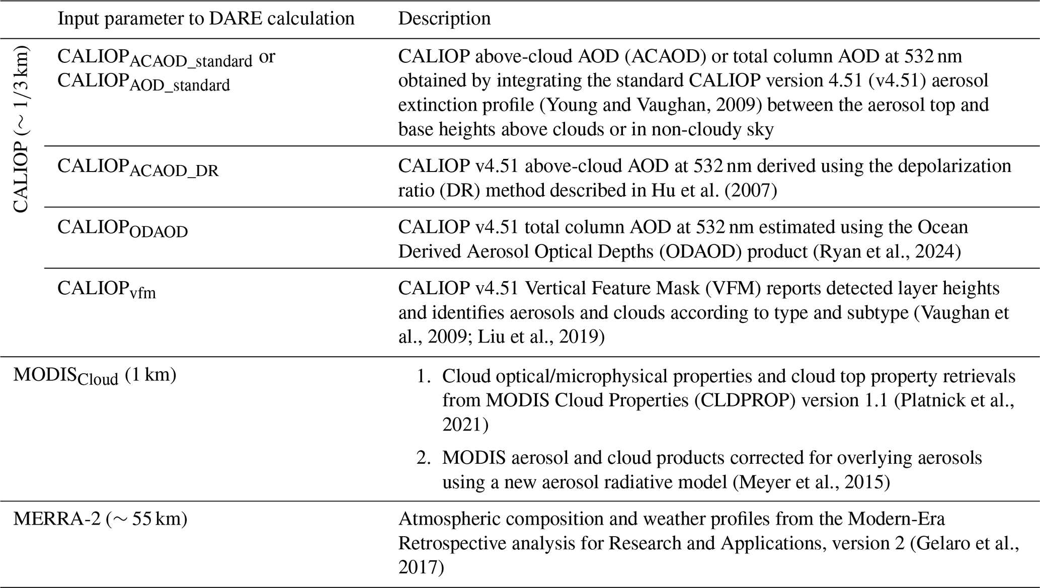
Table 2 Two different DARE calculations (i.e., semi-observational DARE_obs described in Sect. 2.1 and parameterized DARE_param described in Sect. 2.2) in our study and their respective inputs. RRTMG-SW stands for Shortwave Rapid Radiative Transfer Model. See Table 1 for a description of CALIOP_{ACAOD_standard}, CALIOP_{ACAOD_DR}, CALIOP_{AOD_standard}, CALIOP_ODAOD, CALIOP_vfm, MODIS_Cloud, and MERRA-2. n/a: not applicable.

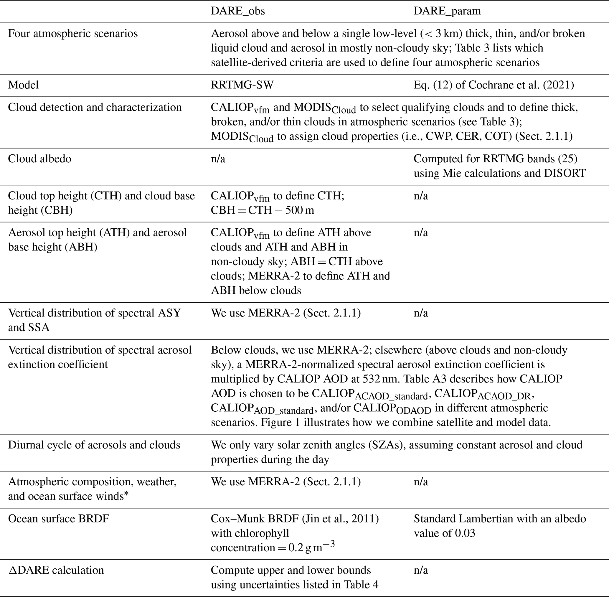
^∗ These parameters are assumed constant along the satellite track: CO₂ volume mixing ratio = 400 ppmv, N₂O mass density = 0.3 ppmv, and CH₄ mass density = 1.7 ppmv. O_{2 mass density}, which is also a required input to RRTMG, is assumed to be 0.0 kg m⁻³. Ocean surface wind variability along the satellite track is provided by MERRA-2. The profiles of temperature, pressure, air density (calculated from pressure and temperature), water vapor, and O₃ vary along the satellite track and are also provided by MERRA-2.

To estimate DARE_obs in Sect. 2.1, we perform solar broadband radiative transfer (RT) calculations using the Shortwave Rapid Radiative Transfer Model for general circulation model (GCM) application (RRTMG-SW) RT code (hereafter, only called RRTMG) (Clough et al., 2005; Iacono et al., 2008) (see Table 2). In RRTMG, gaseous absorption is treated using the correlated-k approach (Mlawer et al., 1997); the delta-Eddington (Joseph et al., 1976) two-stream approximation (Meador and Weaver, 1980; Oreopoulos and Barker, 1999) is used for scattering calculations. Therefore, RRTMG does not need information on the aerosol-phase function, which is why we only use ASY as input. Broadband solar fluxes are calculated from 14 broadbands with bandwidths ranging from 0.2 to 12.0 µm. The four SW RRTMG broadband channels are between 345–442, 442–625, 625–778, and 778–1242 nm. As listed in Table 2, inputs for RRTMG include the optical properties of aerosol and cloud, atmospheric profile, ocean surface BRDF, and solar zenith angle (SZA) information. In RRTMG (using two-stream approximation), total fluxes have an accuracy within 1–2 W m⁻² relative to the standard RRTM-SW (using DISORT) in non-cloudy sky and within 6 W m⁻² in cloudy sky. RRTM-SW with DISORT itself is accurate to within 2 W m⁻² of the data-validated multiple-scattering model, CHARTS (https://github.com/AER-RC/RRTMG_SW, last access: 3 July 2024) (Iacono et al., 2008).

The parameterization that allows us to compute DARE_param is described in Sect. 2.2. It builds on a method that systematically links aircraft observations of Solar Spectral Flux Radiometer (SSFR)-linked spectral fluxes to aerosol optical thickness and other parameters using nine cases from the 2016 and 2017 ORACLES campaigns. This observationally driven link is expressed by a parameterization of the shortwave broadband DARE in terms of the mid-visible AOD and scene albedo.

In this study, we compute both the instantaneous (or instant) DARE along the satellite track for a given location and time and an estimated diurnal average (or 24 h) DARE at the same location that accounts only for the varying solar zenith angle (SZA) throughout the day. We vary SZA corresponding to every hour at the same location and date, compute DARE, and average all instant DARE to obtain 24 h DARE.

2.1 Semi-observational DARE_obs calculations

To design the algorithm that computes DARE_obs, we need to gain an understanding of DARE_obs sensitivities from idealized cases. To do that, we compute a theoretical-based cloudy DARE parameter (i.e., DARE_theo) using RT calculations on several canonical atmospheric cases. Like Table 2 for DARE_obs and DARE_param, Table A1 in the Appendix lists the input parameters to our DARE_theo calculations. DARE_theo is computed for two types of single low warm liquid clouds (i.e., COT = 1, CER = 12, and CWP = 8 vs. COT = 10, CER = 12, and CWP = 80) and varying vertical distributions of RRTMG “built-in” aerosol types (see Fig. A1) while keeping cloud heights, AOD, ASY, atmospheric composition, weather, and ocean surface BRDF constant (see 32 canonical cases illustrated in panels a, b, c, and d of Fig. A2, where we vary the order and amount of two aerosol types over clouds in the vertical). No matter which type and which vertical distribution of aerosol above cloud are considered, DARE_theo values are lower when aerosols are present above a cloud of COT equal to 1 (cases e–b and e–d) compared to a COT equal to 10 (cases e–a and e–c in Fig. A2). This is illustrated by changes of approximatively −7 to −1 W m⁻² for e–b and e–d vs. approximatively 9 to 24 W m⁻² for e–a and e–c of Fig. A2. We also record lower DARE_theo values when adding more scattering aerosols (i.e., “continental” aerosol type) to already absorbing aerosols (i.e., “urban” aerosol type). In effect, DARE_theo values drop from approximatively 24 to 14 W m⁻² when aerosols are more scattering above a cloud of COT equal to 10 (see C1–C4 in e–a vs. C5–C8 in e–a of Fig. A2). And DARE_theo values drop from approximatively −1 to −5 W m⁻² when aerosols are more scattering above a cloud of COT equal to 1 (see C1–C4 in e–b vs. C5–C8 in e–b of Fig. A2). In conclusion, the variability of these DARE_theo calculations confirms, as expected, that our semi-observational DARE_obs calculations need to account for the vertical order and location of aerosol types and aerosol amount.

As listed in Table 2, DARE_obs uses a mix of satellite and model products as input parameters to RRTMG. Section 2.1.1 describes these satellite and model products in further detail. Section 2.1.2 provides more information on how these products are combined. Section 2.1.3 describes how we divide the atmosphere into four atmospheric scenarios along the satellite track. Section 2.1.4 describes the DARE_obs uncertainty calculations.

2.1.1 Data

CALIOP flew on board the CALIPSO platform for 17 years from 2006 to 2023. From its launch in April 2006 until September 2018, CALIPSO flew in tandem with multiple other platforms as part of the A-Train constellation of Earth-observing satellites (Stephens et al., 2018). CALIOP measured high-resolution vertical profiles of attenuated backscatter coefficients (at 532 and 1064 nm) and volume depolarization ratios (at 532 nm) from aerosols and clouds in the Earth's atmosphere from the surface up to ∼40 km. Full instrument details are given in Hunt et al. (2009). A succession of sophisticated retrieval algorithms is used to derive CALIOP Level 2 products from the Level 1 products (Winker et al., 2009). These retrieval algorithms are composed of a feature detection scheme (Vaughan et al., 2009); a module that first distinguishes cloud from aerosol (Liu et al., 2019) and then partitions clouds according to thermodynamic phase (Avery et al., 2020) and aerosols according to subtypes (Kim et al., 2018; Tackett et al., 2023); and, finally, an extinction algorithm (Young et al., 2018) that retrieves profiles of aerosol backscatter and extinction coefficients and the total column AOD based on modeled values of the extinction-to-backscatter ratio (also called lidar ratio) inferred for each detected aerosol layer subtype.

Previous studies have shown that CALIOP standard AOD products underestimate AOD in non-cloudy sky (Kacenelenbogen et al., 2011; Thorsen et al., 2017; Toth et al., 2018) and above clouds (e.g., Kacenelenbogen et al., 2014; Rajapakshe et al., 2017), mostly because CALIOP does not detect tenuous aerosol layers having attenuated backscatter coefficients less than the CALIOP detection threshold (Rogers et al., 2014). The low biases in the total column and above-cloud AODs, denoted in this work as CALIOP_{AOD_standard} and CALIOP_{ACAOD_standard}, respectively (see Table 1; AC stands for above cloud), motivates us to also use two new, independently derived estimates of column optical depth at 532 nm. The first of these uses the depolarization ratio (DR) method developed in Hu et al. (2007), hereafter called CALIOP_{ACAOD_DR} at 532 nm, to calculate total column optical depths above opaque water clouds. By leveraging the unique relationship between layer-integrated volume depolarization (δ_v) and the layer-effective multiple-scattering factor in opaque liquid water clouds (Hu et al., 2006), together with characteristic values of water cloud lidar ratios, an accurate estimate of the opaque water cloud integrated attenuated backscatter in non-cloudy sky (γ′_clear) can be obtained (Platt, 1973). The two-way transmittance due to aerosols above the cloud (and hence above-cloud optical depth) is thus obtained by dividing the measured cloud integrated attenuated backscatter, γ′_measured, by the γ′_clear estimate. As of CALIOP's version 4.51 data release, CALIOP_{ACAOD_DR} retrievals are now included as a standard scientific dataset (SDS) contained in the layer products for all averaging resolutions. However, the individual components required for the DR method (e.g., δ_v and γ′_measured) were routinely reported in earlier data releases, and hence AODs derived using the DR method have been used extensively in previous studies (e.g., Chand et al., 2008; Liu et al., 2015; Kacenelenbogen et al., 2019). Furthermore, comparisons made by Ferrare et al. (2017) show that CALIOP_{ACAOD_DR} agrees well (bias and RMS differences less than 0.05 % and 10 %) with coincident measurements by the NASA Langley Research Center airborne high-spectral-resolution lidars (HSRLs) during two flights (18 and 20 September 2016) of the ORACLES field campaign (Redemann et al., 2021). The second of CALIOP's independently derived total column AOD estimates is provided by the Ocean Derived Column Optical Depths (ODCOD) algorithm (Ryan et al., 2024), hereafter called CALIOP_ODAOD at 532 nm. As with the DR method estimates, the ODCOD AOD is a new parameter reported for the first time in CALIOP's v4.51 data release. ODCOD works by comparing an idealized parameterization of laboratory measurements of the 532 nm detector impulse response function (IRF) to space-based measurements of the backscattered energy from the ocean surface. Similar in operation to the technique employed by Venkata and Reagan (2016), the ODCOD algorithm shifts the IRF model in time and scales it in magnitude to achieve the best fit to the measured data. When weighted by surface wind speed, the area under the curve of this shifted and scaled model is directly related to the attenuation of the laser surface return by the intervening atmosphere. Note that both ODCOD and the DR method report effective optical depths, that is, the product of the true overlying optical depths and a column-effective multiple-scattering factor, η_col, where $\mathrm{0}<{\mathit{\eta }}_{\mathrm{col}}\le \mathrm{1}$. Because ODCOD AODs are retrieved immediately after executing the CALIOP surface detection algorithm, and prior to conducting a search for atmospheric layers, no attempt is made to separate multiple-scattering and single-scattering contributions made by the overlying particulates (i.e., clouds and/or aerosols). Fortunately, in cloud-free columns containing only aerosol layers, η_col≈1 (Young et al., 2018). Consequently, multiple-scattering corrections are neglected in the standard extinction retrieval (Winker et al., 2009) and considered unnecessary in the ODCOD analyses. The extensive comparisons shown in Ryan et al. (2024) demonstrate that CALIOP_ODAOD agrees well with coincident HSRL measurements during all CALIOP-HSRL co-located flights from 2006 to 2022. The median difference in the daytime between CALIOP_ODAOD and HSRL AOD is $-\mathrm{0.037}\pm \mathrm{0.052}$ ($-\mathrm{12}\pm \mathrm{25}$ %; N=149), with CALIOP_ODAOD being lower and a correlation coefficient of 0.775.

In our study, as listed in Table 2, we use CALIOP to characterize aerosol optical depth above clouds (CALIOP_{ACAOD_standard}, CALIOP_{ACAOD_DR}) and in cloud-free skies (CALIOP_{AOD_standard} and CALIOP_ODAOD) to establish aerosol and cloud top heights (CALIOP_vfm; vfm stands for Vertical Feature Mask) and as the source of the SZAs in our DARE_obs calculations. Table A3 describes how CALIOP AOD is chosen to be equal to CALIOP_{ACAOD_standard}, CALIOP_{ACAOD_DR}, CALIOP_{AOD_standard}, and/or CALIOP_ODAOD in different atmospheric scenarios (i.e., non-cloudy sky or among thick and/or thin clouds present). We also use the latest CALIOP stratospheric aerosol profile product (version 1.00; Kar et al., 2019) to correct for attenuation by stratospheric aerosols in CALIOP_{ACAOD_DR} and CALIOP_ODAOD. To do that, we compute a zonal climatology of stratospheric aerosol optical depth (SAOD) from the equal-angle data product, then interpolate the zonal data to the latitude grid of the CALIPSO granule observations (see Fig. A3 in the Appendix). Finally, we subtract the SAOD from CALIOP_{ACAOD_DR} and CALIOP_ODAOD. Note that while performing our DARE_theo calculations, we confirmed the importance of considering stratospheric aerosols. Adding stratospheric aerosols between 25–30 km with a typical AOD value of 0.04 in the stratosphere (Kloss et al., 2021) to tropospheric aerosols above clouds leads to an absolute difference in DARE_theo of up to 3.7 W m⁻². We also use CALIOP_vfm to select clouds of interest (i.e., single-layer low warm liquid clouds) and to define thick, broken, and/or thin clouds in our four atmospheric scenarios described in Sect. 2.1.3.

MODIS/Aqua flew as part of the A-Train constellation of satellites from 2002 until a final drag makeup satellite maneuver in December 2021, after which Aqua began a slow descent below the A-Train. MODIS has 20 shortwave spectral bands from 412 to 2130 nm, along with 16 infrared bands from 3.7 to 14.4 µm, enabling retrievals of the macrophysical, microphysical, and radiative properties of clouds. CER is commonly retrieved simultaneously with COT from passive imager remote sensing observations using a bi-spectral technique (Nakajima and King, 1990; Platnick et al., 2003), pairing a non-absorbing visible or near-infrared spectral channel sensitive to COT with an absorbing shortwave infrared or mid-wave infrared spectral channel sensitive to CER. In this paper, we use two types of cloud products from MODIS (referred to as MODIS_Cloud in Table 1). The first type of MODIS_Cloud product is from the current operational algorithm and does not account for the presence of aerosols above clouds (Meyer et al., 2013). These are called uncorrected MODIS_Cloud products in this paper and are derived from the Cross-platform HIgh resolution Multi-instrument AtmosphEric Retrieval Algorithms (CHIMAERA) shared-core suite of cloud algorithms (Wind et al., 2020). This suite of algorithms includes cloud optical/microphysical properties (e.g., thermodynamic phase, optical thickness, particle effective size, water path) and cloud top property retrievals from the MODIS/Visible Infrared Imaging Radiometer Suite (VIIRS) CLDPROP version 1.1, designed to sustain the long-term records of MODIS (cloud property continuity product) (Platnick et al., 2021). The second type of MODIS_Cloud product derives from a new retrieval technique that corrects the MODIS cloud retrievals by accounting for overlying aerosols. These are called corrected MODIS_Cloud products in this paper. In Grosvenor et al. (2018), comparisons between MODIS and the Advanced Microwave Scanning Radiometer 2 (AMSR2), which is not sensitive to the above-cloud aerosol, indicate derived cloud droplet number concentration differences of <10 cm⁻³ over most of the southeast Atlantic stratocumulus deck. As described in Meyer et al. (2015), what we call corrected MODIS_Cloud in this paper was achieved by adding aerosols with prescribed scattering properties in the radiative transfer calculations that are used to construct bi-spectral lookup tables. Note that this correction is strongly dependent on the assumed aerosol scattering properties. For this study, these properties are derived from the NASA Spectrometers for Sky-Scanning Sun-Tracking Atmospheric Research (4STAR) observations obtained during ORACLES 2016. Since the cases we carefully selected for DARE_obs are also during the deployment of ORACLES, we can assess the effects of using either corrected or uncorrected MODIS_Cloud properties in DARE_obs calculations (see Sect. 2.1.4). The main cloud properties needed in the DARE_obs calculations are CWP, CER, and COT (see Table 2).

Regardless of the cloud product used, validating retrievals such as COT, CER, and CWP is difficult, as there are no direct measurements of these radiative quantities. Microphysical retrievals can be compared against airborne in situ cloud probes, and previous investigations have found notable differences, though strong correlation, between the two, with MODIS-derived CER on average more than 2 µm larger than that derived from legacy in situ probes (e.g., Nakajima et al., 1991; Platnick and Valero, 1995; Painemal and Zuidema, 2011; Min et al., 2012; King et al., 2013; Noble and Hudson, 2015; Gupta et al., 2022). Other studies using probes leveraging different observation techniques (e.g., Witte et al., 2018) have shown no systematic differences in CER. Comparisons against other retrieval techniques, such as polarimetry, can also inform CER retrieval quality. Using ORACLES airborne observations, Meyer et al. (2025) performed an extensive comparison of spectral imager liquid CER retrievals (from the Enhanced MODIS Airborne Simulator, eMAS, an airborne proxy instrument of MODIS, and the Research Scanning Polarimeter, RSP) with those from polarimetry (from RSP) and CER derived from two in situ cloud probes. Agreement between the imager, polarimetric, and probe-derived CER was found to be case and spectral dependent, and accounting for above-cloud aerosol absorption in the bi-spectral imager retrievals (equivalent to using corrected MODIS_Cloud) either has no impact or worsens the agreement depending on the spectral channel used. In Sect. 2.1.4, we demonstrate that correcting cloud properties for aerosol above them leads to insignificant differences in mean instant DARE_obs values (up to 4 W m⁻²) for all three case studies.

Like other papers (e.g., Su et al., 2013), and because satellites are not yet well suited to broadly observe the vertical profile of aerosol intensive properties, we use NASA's Global Modeling and Assimilation Office (GMAO) MERRA-2 to complement satellite observations. MERRA-2 data became available in September 2015 (Gelaro et al., 2017), covering 1980–present. It is based on a version of the GEOS-5 atmospheric data assimilation system that was frozen in 2008 and was produced on a 0.5×0.625° grid (∼55 km × 69 km) on 72 hybrid sigma–pressure coordinate system vertical levels. It was frozen so that the underlying model physics, schemes, and data assimilation techniques are the same for the duration of the MERRA-2 reanalysis. It uses a version of the Goddard Chemistry Aerosol Radiation and Transport (GOCART) model (Chin et al., 2002; Colarco et al., 2010, 2014) to treat the emission, transport, removal, and chemistry of dust, sea salt, sulfate, and carbonaceous aerosols. Aerosol optical properties are computed from the Mie-theory-based Optical Properties of Aerosol and Cloud (OPAC) dataset (Hess et al., 1998), except for dust, which was derived by an observation-derived dataset of refractive indices and an assumption of a spheroidal shape, as described in Colarco et al. (2014). MERRA-2 assimilates satellite, air, and ground observations (Randles et al., 2017) to constrain both the atmospheric and the aerosol states in the model. MERRA-2 also provides optical properties within the SW RRTMG broadband channels. As listed in Table 2, our DARE_obs calculations use MERRA-2 (GMAO, 2015) ocean surface wind, ozone, temperature, pressure, air density, and water vapor profiles, as well as aerosol intensive properties (i.e., spectral extinction coefficient, SSA, ASY) above and below low opaque water clouds and in non-cloudy sky. We use CALIOP AOD quantities at 532 nm, and we populate the 442–625 nm RRTMG channel with an observational AOD value. We then spectrally extrapolate the AOD at 532 nm in the other broadband RRTMG channels of the shortwave part of the spectrum using the MERRA-2 spectral shape of extinction coefficients, as further described in Sect. 2.1.2. Many papers have shown that MERRA-2 aerosol extensive and intensive properties and horizontal/vertical distribution are far from perfect (e.g., Nowottnick et al., 2015). For example, GEOS aerosol single-scattering albedo (SSA) was shown to be consistently higher than that of in situ measurements during the ORACLES field campaign, explained by an underestimation of BC content by the GEOS model (Das et al., 2024). We expect, according to the DARE_theo calculations illustrated in Fig. A2, that a high bias in the MERRA-2-estimated SSA, if not compensated for by other factors, would cause a low bias in DARE_obs calculations (see, for example, lower DARE_theo values in e–a for C5–C8, where SSA is higher compared to higher DARE_theo values in e–a for C1–C4, where SSA is lower). As CALIOP cannot reliably provide any aerosol information below clouds due to signal attenuation, we also use MERRA-2 to inform aerosol extensive and intensive properties and layer heights below clouds.

Finally, we must assume a consistent observed and modeled extinction coefficient threshold under which we consider that there is no aerosol present in the atmosphere. Based on Rogers et al. (2014), we consider that there are no aerosols (and hence DARE_obs = 0) if the CALIOP extinction coefficient at 532 nm is below 0.07 km⁻¹. As the lower threshold on the CALIOP extinction of 0.07 km⁻¹ is based on an aerosol layer that is 1.5 km thick in Rogers et al. (2014), we impose a lower threshold on MERRA-2 extinction of 0.014 km⁻¹ in the 442–625 nm RRTMG broadband channel. This is because the MERRA-2 layers are, on average, 0.29 km thick in September 2016 in a MERRA-2 grid box located at −10° W to 10° E and −40° S to 0° and between 1–5 km altitude. In Sect. 2.1.4, we demonstrate that adding or removing such a threshold on the aerosol extinction coefficient leads to insignificant differences in mean instant DARE_obs values (up to 0.8 W m⁻²) for all three case studies.

2.1.2 Combination of satellites and model

In this subsection, we show how we combine the satellite products with modeled data to perform RT calculations that represent DARE_obs. As described in Table 2, on the one hand, MODIS and CALIOP satellites are used to detect and characterize clouds, define aerosol height, and provide aerosol extinction coefficients above clouds and in non-cloudy sky. MERRA-2, on the other hand, is used to define aerosol top and base heights below clouds and provide the vertical distribution of spectral ASY, SSA, and extinction coefficient above and below clouds and in non-cloudy skies, along with information about atmospheric composition, weather, and ocean surface winds. We emphasize that we use MERRA-2 aerosol and atmospheric data regardless of any MERRA-2-simulated clouds (i.e., we do not use MERRA-2 cloud simulations in any way, nor do we assess cloud agreement between MERRA-2 and satellite observations in this paper).

First, we collocate MODIS and CALIOP satellite observations every 1 km horizontally along CALIOP's track using the method described in Nagle and Holz (2009). By doing this, we account for the parallax effect, i.e., the cloud top height dependence on spatial co-location. Using a simple surface collocation method that does not account for the parallax effect could result in a horizontal shift of more than 5 pixels (Holz et al., 2008).

Second, to compute DARE_obs, we need to combine aerosol extensive properties primarily obtained from CALIOP with aerosol intensive properties primarily obtained from MERRA-2. Figure 1 illustrates the combination of CALIOP and MERRA-2 products above clouds and in non-cloudy sky. In the green region in Fig. 1a, we assume one or multiple aerosol layer(s) of different aerosol types contained between the uppermost CALIOP-informed aerosol top and the lowermost CALIOP-informed aerosol base heights. The AOD at 532 nm, corresponding to the vertical integration of the extinction coefficients of these single or multiple aerosol layers, is obtained from CALIOP (called AOD_C) in Fig. 1 (i.e., CALIOP_{ACAOD_standard}, CALIOP_{ACAOD_DR}, CALIOP_{AOD_standard}, or CALIOP_ODAOD – see Table 1). The illustrative MERRA-2 profile in Fig. 1b, collocated in space and time with the profile in Fig. 1a, shows three aerosol layers in blue, orange, and yellow on an initial (and uneven) MERRA-2 vertical grid. It also shows six “aerosol-free” MERRA-2 aerosol layers in hashed grey (i.e., aerosol layers for which MERRA-2 extinction coefficients are below 0.014 km⁻¹ in the 442–625 nm RRTMG broadband channel). We refer to L, the number of MERRA-2 aerosol layers (L=3 in Fig. 1b). In each vertical layer, i, and for each RRTMG broadband channel, λ, we record the MERRA-2 extinction coefficient, σ_M(i,λ); MERRA-2 SSA, SSA_M(i,λ); and MERRA-2 ASY, ASY_M(i,λ), in Fig. 1b. To combine CALIOP and MERRA-2 (Fig. 1c), we keep L constant and do not allow “aerosol-free” layers (hashed grey) to physically touch either the CALIOP-inferred aerosol top or the aerosol base heights. Combined CALIOP and MERRA-2 (C-M) SSA_C-M(i,λ) and ASY_C-M(i,λ) are equal to MERRA-2 SSA_M(i,λ) and ASY_M(i,λ), respectively. The combined CALIOP and MERRA-2 extinction coefficients, σ_C-M(i,λ), are computed as in Eq. (2):

$$\begin{array}{}\text{(2)}& \begin{array}{rl}{\mathit{\sigma }}_{\text{C-M}}\left(i,\mathit{\lambda }\right)& =\left({\displaystyle \frac{{\text{AOD}}_{\mathrm{C}}\left(\mathrm{532}\mathrm{nm}\right)}{L}}\right)\\ & \times \left({\displaystyle \frac{{\mathit{\sigma }}_{\mathrm{M}}\left(i,\mathit{\lambda }\right)}{{\mathit{\sigma }}_{\mathrm{M}}\left(i,\mathrm{442}-\mathrm{625}\mathrm{nm}\right)}}\right).\end{array}\end{array}$$

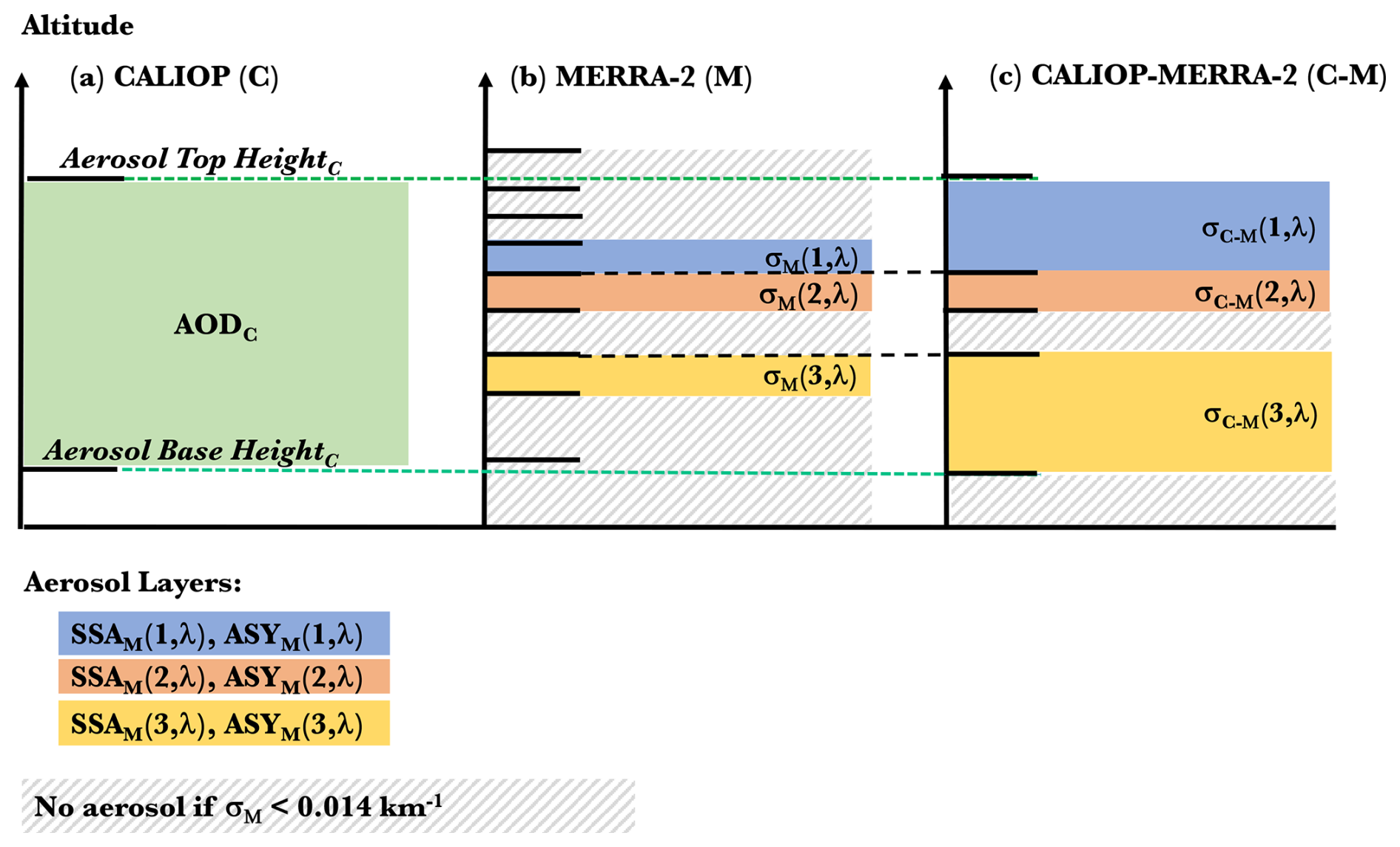
Figure 1 Illustration of how we combine MERRA-2 and CALIOP above clouds and in non-cloudy sky. In green in (a), we assume one or multiple aerosol layers contained between a CALIOP-inferred aerosol uppermost layer top height and aerosol lowermost base height. The AOD of the aerosol plume in green is informed by CALIOP at 532 nm, AOD_C. Panel (b) is the MERRA-2 profile collocated in time and space with the CALIOP profile in (a). The MERRA-2 profile in (b) shows three aerosol layers (blue, orange, and yellow) for which the MERRA-2 extinction coefficient, SSA, and ASY are called σ_M(i,λ), SSA_M(i,λ), and ASY_M(i,λ), respectively, in each layer i and in each broadband RRTMG channel λ. The combined CALIOP and MERRA-2 profile in (c) records SSA_M(i,λ), ASY_M(i,λ), and σ_C-M(i,λ) as computed using Eq. (2).

2.1.3 DARE_obs for four atmospheric scenarios

Based on our theoretical calculations (see Table A1 and Fig. A2) and previous studies such as Matus et al. (2019), DARE results are clearly dependent on cloud thickness and cloud spatial homogeneity. To evaluate DARE, we generalize the atmospheric conditions into four scenarios based on different cloud conditions. In assembling our combined CALIPSO + MODIS dataset, we start by removing records that report clouds of any types and at any altitudes above the single low warm liquid cloud (LWLC) that is closest to the Earth's surface (i.e., any clouds above a top height of 3 km). The first three scenarios show aerosol above and below different types of LWLC, and the fourth scenario shows aerosol in (possibly cloud-contaminated) non-cloudy sky. We define the geometrical thickness and spatial uniformity of LWLC using both CALIOP and MODIS cloud properties. Table 3 defines our nomenclature for different types of LWLCs moving forward, how each type is characterized using CALIOP and MODIS data, and in which scenario they can be present.

Table 3 Method to distinguish a single low warm liquid cloud (LWLC) in atmospheric scenarios S1, S2, S3, and S4 using MODIS_Cloud and CALIOP_vfm (see Table 1). For all scenarios, we collocate MODIS and CALIOP every 1 km along the CALIOP track using the method described in Nagle and Holz (2009). Profiles are deleted if high clouds are present with CALIOP cloud top height >3 km, and clouds are “highly confident” when 111> CALIOP cloud–aerosol discrimination (CAD) >20, CALIOP cloud temperature $>-\mathrm{10}$ °C, CALIOP phase quality assurance ≥2, and CALIOP cloud phase = 2. n/a: not applicable.

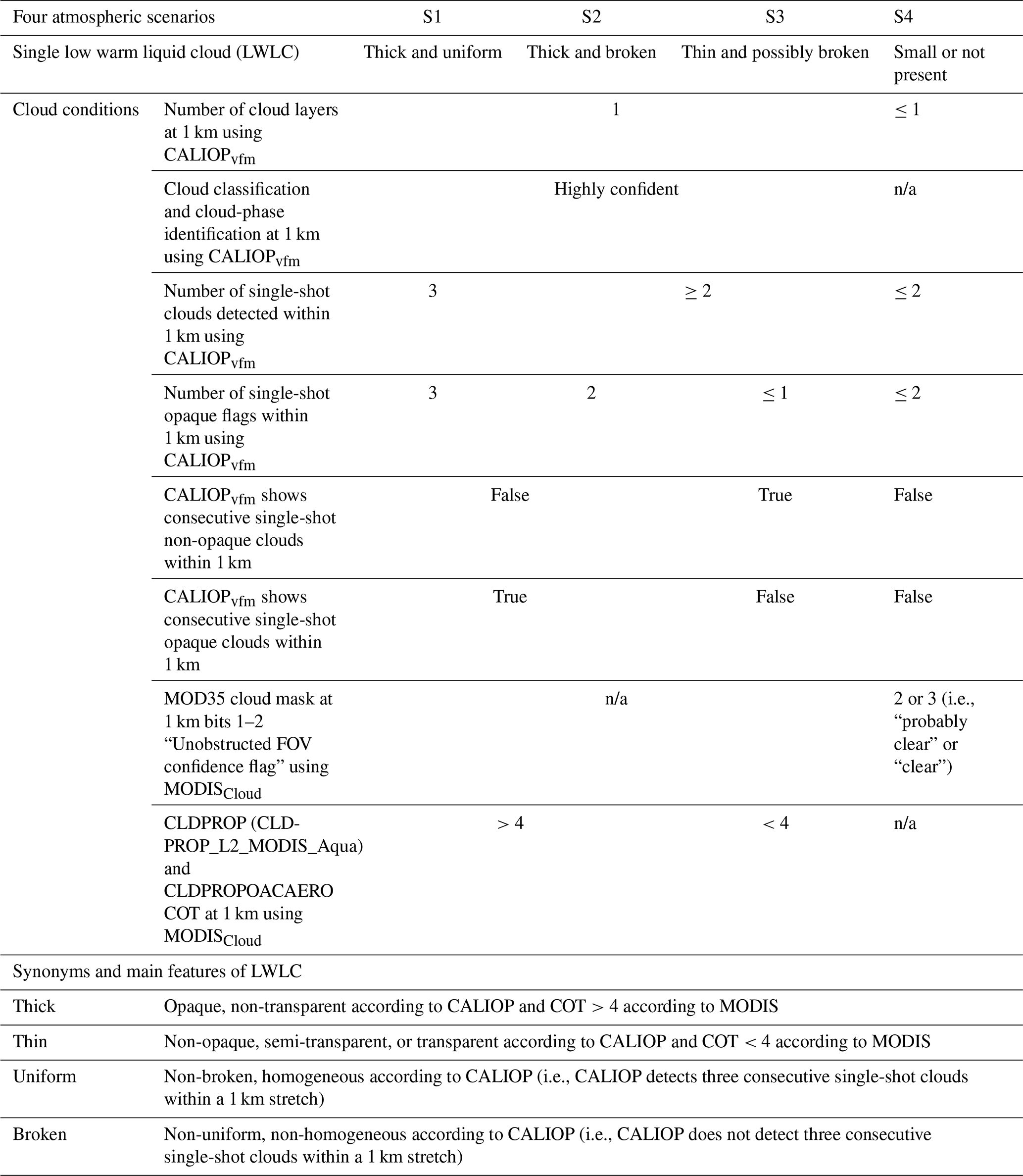
Table A3 in the Appendix describes which aerosol (derived from CALIOP and/or MERRA) and cloud parameters (derived from MODIS) were used and how these parameters were filtered to compute DARE_obs in the case of S1, S2, S3, and S4.

We compute DARE_obs using the input parameters in Table 2 and for each 1 km stretch, to which a particular atmospheric scenario is attributed in Table 3. We then regroup all these DARE_obs results along the track to obtain daily and, eventually, regional, monthly, seasonal, and/or yearly DARE_obs statistics.

When clouds are present in the atmosphere, DARE_obs of aerosol above clouds (i.e., DARE_cloudy for S1, S2, and S3 combined) is the subtraction of upward fluxes for clouds without aerosols and for clouds with aerosols above them. If we have N1 × S1, N2 × S2, and N3 × S3 cases along track, where NX represents the number of cases occurring for scenario SX, then we compute DARE_cloudy as follows:

$$\begin{array}{}\text{(3)}& {\mathrm{\text{DARE}}}_{\mathrm{cloudy}}={\displaystyle \frac{\sum _{i=\mathrm{1}}^{\mathrm{N}\mathrm{1}}{\mathrm{DARE}}_{\mathrm{S}\mathrm{1},i}+\sum _{j=\mathrm{1}}^{\mathrm{N}\mathrm{2}}{\mathrm{DARE}}_{\mathrm{S}\mathrm{2},j}+\sum _{k=\mathrm{1}}^{\mathrm{N}\mathrm{3}}{\mathrm{DARE}}_{\mathrm{S}\mathrm{3},k}}{\text{N1}+\text{N2}+\text{N3}}}.\end{array}$$

When clouds are absent in the atmosphere, DARE_obs of aerosol in non-cloudy sky (i.e., DARE_non-cloudy for scenario S4) is the subtraction of upward fluxes for non-cloudy sky without aerosols and non-cloudy sky with aerosol present. If we have N4 × S4 cases, we compute DARE_non-cloudy as follows:

$$\begin{array}{}\text{(4)}& {\text{DARE}}_{\text{non-cloudy}}={\displaystyle \frac{\sum _{l=\mathrm{1}}^{\mathrm{N}\mathrm{4}}{\mathrm{DARE}}_{\mathrm{S}\mathrm{4},l}}{\text{N4}}}.\end{array}$$

To be consistent with the assumptions in the RT used for the MODIS COT retrieval (i.e., MODIS assumes CF = 1 to retrieve COT), we assign MODIS CF values of 1 for S1, S2, and S3 and 0 for S4. Finally, we compute DARE in all-sky conditions (DARE_all  sky for scenarios S1, S2, S3, and S4) as follows:

$$\begin{array}{}\text{(5)}& {\text{DARE}}_{\text{all\hspace{0.17em}\hspace{0.17em}sky}}={\displaystyle \frac{\begin{array}{c}{\mathrm{\text{DARE}}}_{\mathrm{cloudy}}\times \left(\text{N1}+\text{N2}+\text{N3}\right)\\ +{\text{DARE}}_{\text{non-cloudy}}\times \text{N4}\end{array}}{\text{N1}+\text{N2}+\text{N3}+\text{N4}}}.\end{array}$$

2.1.4 DARE_obs uncertainties

We vary AOD, CWP, SSA, ASY, and surface albedo according to their uncertainties in our DARE_obs calculations to obtain the DARE_obs uncertainties. Table 4 describes the assumed or computed uncertainties used on these five input parameters to DARE_obs.

Table 4 Input uncertainties in AOD, CWP, SSA, ASY, and surface albedo used in our DARE_obs uncertainty calculation. See Table 1 for the definitions of CALIOP_{ACAOD_standard}, CALIOP_{AOD_standard,} CALIOP_{ACAOD_DR,} MODIS_Cloud, and MERRA-2 and Table 2 on how these input parameters are used to computed DARE_obs.

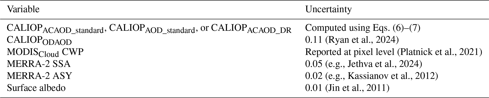
Regarding uncertainties in the AOD values, we use Eqs. (6) and (7) described below to compute an uncertainty in CALIOP_{ACAOD_standard}, CALIOP_{AOD_standard}, and CALIOP_{ACAOD_DR} for each 20 km stretch. We assume a Gaussian distribution of N single-shot samples x₁, …, x_N (e.g., CALIOP_{ACAOD_standard}, CALIOP_{AOD_standard}, or CALIOP_{ACAOD_DR}), with each sample x_i recording a single-shot uncertainty σ_i reported by the CALIOP team. We compute a weighted mean μ over a 20 km stretch as follows:

$$\begin{array}{}\text{(6)}& \mathit{\mu }={\displaystyle \frac{{\sum }_{i=\mathrm{1}}^N\left(\frac{x_i}{{\mathit{\sigma }}_i^{\mathrm{2}}}\right)}{{\sum }_{i=\mathrm{1}}^N\left(\frac{\mathrm{1}}{{\mathit{\sigma }}_i^{\mathrm{2}}}\right)}},\end{array}$$

where the weighting factor is the inverse square of the error, $\mathrm{1}/{\mathit{\sigma }}_i^{\mathrm{2}}$. Note that the smaller the uncertainty, the larger the weight and vice versa. The error in the weighted mean can be computed as follows (Bevington and Robinson, 1992):

$$\begin{array}{}\text{(7)}& {\mathit{\sigma }}^{\mathrm{2}}\left(\mathit{\mu }\right)={\displaystyle \frac{\mathrm{1}}{{\sum }_{i=\mathrm{1}}^N\left(\frac{\mathrm{1}}{{\mathit{\sigma }}_i^{\mathrm{2}}}\right)}}.\end{array}$$

When filtering for ocean surface wind speeds between 3 and 15 m s⁻¹ in Ryan et al. (2024), CALIOP_ODAOD values have an averaged uncertainty of $\sim \mathrm{0.11}\pm \mathrm{0.01}$ (75±37 % relative) day and night. This uncertainty is mostly due to ocean surface wind speed. In our study, we average CALIOP_ODAOD over 20 km stretches, for which the ocean surface wind speed remains constant because we use MERRA-2 with a horizontal resolution of ∼55 km. Therefore, in our study, we use a constant value of 0.11 for the averaged uncertainty in CALIOP_ODAOD. We use reported uncertainties at the pixel level in CWP (Platnick et al., 2021). As for uncertainties in the aerosol intensive properties, we use an uncertainty of 0.05 for SSA and 0.02 for ASY. The averaged SSA uncertainty of 0.05 is inspired by Jethva et al. (2024), who developed a novel synergy algorithm that combines direct airborne measurements of above-cloud aerosol optical depth and the TOA spectral reflectance from the Ozone Monitoring Instrument (OMI) and MODIS sensors. It shows, in its Table 3, a maximum absolute uncertainty of −0.054 in the retrieved near-UV SSA for an error of −40 % (underestimation) in ACAOD results. The averaged ASY uncertainty of 0.02 is inspired by Fig. 9 in Kassianov et al. (2012), who investigate the expected accuracy of 4STAR. It describes the relative difference between “true” and retrieved values of ASY for 4 selected days and shows a maximum of ±0.02 uncertainty for ASY at 1.02 µm, which becomes smaller at shorter wavelengths. Finally, we assume an averaged uncertainty of 0.01 in the surface albedo, inspired by Fig. 10 in Jin et al. (2011), in which they find a standard deviation of ∼0.01 between measured and parameterized broadband shortwave albedo for 2 years (2000–2001).

For each 1 km stretch, we compute DARE_obs using the uncertainty ranges of each variable (see Table 4), compute upper and lower bounds for DARE_obs, and then combine these values to get the DARE_obs uncertainty.

While designing our algorithm, we evaluated the effects of a few constraints in the computation of our final DARE_obs results. The effects are identified by (E-1) through (E-6) in Table A3 and quantified in Table A4 in the Appendix. We separate these effects into five categories – the effects of (E-1) adding a lower threshold on extinction coefficients, (E-2) adding aerosol information below clouds, (E-3) spatially extending aerosol top height information, (E-4) using AOD version 2 along track, (E-5) using AOD version 3 along track, and (E-6) using corrected clouds instead of uncorrected clouds for overlying aerosols.

Regarding categories (E-1), (E-2), and (E-3), the effects add up to a small N=10 data points at 1 km in Table A4 and lead to a small difference in mean instant all-sky (S1–S4) DARE_obs of maximum ∼1.6 W m⁻².

Regarding categories (E-4) and (E-5), we computed DARE_obs using three AOD versions (we call these v1, v2, and v3 – see Table A3) and evaluated the differences they make in the number of 1 km data points and in the mean DARE_obs values. The latitudinal evolution of AOD v1, v2, and v3 along the CALIOP track is illustrated in Fig. A4 in the Appendix. Using AOD v2 instead of AOD v1 adds up to N=65 data points at 1 km in Table A4 and makes a difference in mean instant all-sky (S1–S4) DARE_obs of maximum ∼1.3 W m⁻². Using AOD v3 instead of AOD v2 makes the most difference in mean instant all-sky DARE_obs (i.e., up to 3.2 W m⁻² difference in DARE_obs on 13 August 2017).

Regarding category (E-6), using corrected vs. uncorrected clouds paired with AOD >0.3 leads to a difference in mean instant above-thick-cloud (S1) DARE_obs values up to ∼4.1 W m⁻² on 20 September 2016 (comparison shown in more detail in Fig. A5 and Table A5 in the Appendix). Applying a correction to the clouds does not seem to matter much in our study regarding DARE_obs or COT. We argue that this is likely due to the generally low AOD values on all 3 days. Note that we would probably notice a significant difference in DARE_obs when clouds are corrected vs. uncorrected if we were to apply our DARE_obs calculations to multiple years over the region of the southeast Atlantic.

In the end, the effects of (E-1) through (E-6) all lead to small differences in DARE_obs below a threshold of 6 W m⁻², which represents the accuracy of total fluxes in overcast conditions when comparing RRTMG-SW with other radiative transfer schemes (such as RRTM-SW). We emphasize that the DARE_obs results in Sect. 3 apply a lower threshold on the extinction coefficients (E-1), use aerosols below clouds (E-2), extend the ATH when possible (E-3), use CALIOP-inferred AOD version 2, and use cloud properties from MODIS that are uncorrected for aerosols above them (E-6).

2.2 Parameterized DARE_param calculations

The DARE_param (see Table 2) parameterization framework in this section was developed by Cochrane et al. (2021) (see their Eq. 12). It collectively used airborne observations from the ORACLES field campaigns over the southeast Atlantic in conjunction with DARE calculations to derive statistical relationship between (a) DARE and (b) aerosol and cloud properties. DARE_param supports a minimal parameterization for the entire ORACLES campaign. Specifically, for a range of SZAs, within the southeast Atlantic region and during ORACLES (nine cases from the 2016 and 2017 ORACLES deployments to be exact), it links a broadband instant DARE_param estimate for typical biomass burning aerosols injected above an omnipresent stratocumulus deck and in non-cloudy sky to two driving parameters, which are (i) a measure of the AOD (i.e., in our study, a combination of CALIOP_{ACAOD_standard}, CALIOP_{ACAOD_DR}, CALIOP_{AOD_standard}, and CALIOP_ODAOD at 532 nm) and (ii) a measure of the albedo of the underlying surface (i.e., either clouds or the ocean surface). Cochrane et al. (2021) report that their DARE_param possesses a 20 % uncertainty (lower bound on DARE variability) and that this uncertainty is due to factors other than AOD and scene albedo, such as measurement uncertainty and spatial/temporal variability of the cloud and aerosol properties. Note that, had we had a satellite retrieval of SSA with minimal uncertainty, we could have reduced the uncertainty in DARE_param by using the second parameterization in Cochrane et al. (2021) that requires SSA in addition to the AOD and the scene albedo. The advantage of DARE_param is that it establishes a direct link between DARE and two driving parameters, and it circumvents the need for radiative transfer calculations, aerosol composition, aerosol and cloud top height, atmospheric profiles, or ocean surface wind information, which are required to compute semi-observational DARE_obs in our study (see Table 2). We emphasize that this parameterization only represents the relationship between DARE and aerosol and cloud properties as sampled over the ORACLES study region and during the ORACLES time frame. Outside of this framework (i.e., other regions of the globe and other seasons), different aerosol and cloud types can alter the DARE to cloud and aerosol relationship. To our knowledge, there are no current plans to extend the parameterization behind DARE_param to other times and regions of the globe. Consequently, we will not be able to assess global DARE_obs results in future studies using DARE_param. In Sect. 3.3.1, we compare instant DARE_obs and DARE_param as a first way to evaluate our results.

3 Results

First, we describe the atmospheric scenes during three suborbital ORACLES flights (Sect. 3.1). Second, we analyze the temporal and spatial variability of aerosol, cloud properties, and all-sky DARE_obs during these suborbital flights (see Sect. 3.2). Third, we evaluate DARE_obs results (Sect. 3.3) using two methods – collocated DARE_param (Sect. 3.3.1) and airborne SSFR upward spectral irradiance measurements (Sect. 3.3.2).

3.1 Suborbital flights for evaluation

Figure 2 illustrates our three case studies offshore from Namibia, southern Africa. The MODIS RGB images in Fig. 2 show an omnipresent stratocumulus deck on all 3 days but a variability in cloud types along the CALIOP track (i.e., broken, uniform, thick, and/or thin – see Table 3). It also shows aerosol plumes of different loadings on all 3 days, with CALIOP AOD overlaid along the track from 0.01 (dark blue) to above 1 (dark red). On each day, both a high-flying plane focusing on remote sensing and a low-flying plane focusing on in situ sampling were deployed (Redemann et al., 2021). By 18 and 20 September 2016, strengthened westward free-tropospheric winds dispersed aerosol broadly over the stratocumulus deck, up to an altitude of 6.0 km (Redemann et al., 2021; Ryoo et al., 2021). The highest aerosol loadings of ORACLES 2016 were recorded on 20 September (Pistone et al., 2019; Redemann et al., 2021). The highest AOD values (i.e., >0.5) are clearly visible on 20 September 2016 in Fig. 2. The aerosol loadings reached maximums during the day and diminished towards sunrise and sunset (Ryoo et al., 2021). The SSA is approximately 0.85 on 20 September 2016 at a wavelength of 500 nm, based on both in situ and SSFR retrievals (Pistone et al., 2019). During 13 August 2017, the aerosol was located lower, within a drier (RH <60 %) layer with its top at 3 km, resting on top of a thinner cloud deck transitioning from overcast to broken. Smoke aerosol was also sampled in the boundary layer on 13 August 2017 (Zhang and Zuidema, 2019). The CALIOP track is well aligned with the high-altitude ER-2 aircraft (in light blue) on the first 2 days and with the lower-altitude P3 aircraft (in darker blue) on the third day, which was purposely achieved by flight planning beforehand. Among the instruments flying on board the ER-2, the HSRL-2, RSP, and eMAS instruments are usually used to evaluate aerosol and cloud properties retrieved from CALIOP and/or MODIS. Note that we do not use measurements from these airborne instruments in this paper. Among the many instruments flying on board the P3 aircraft, our focus is on the Solar Spectral Flux Radiometer (SSFR) instrument (Pilewskie et al., 2003; Schmidt and Pilewskie, 2012), which we use to evaluate our DARE_obs results in Sect. 3.3.2. We remind the reader that in this paper, we use the observations and the modeled parameters listed in Table 2 (i.e., MODIS for cloud microphysics; CALIOP for AOD and cloud and aerosol heights; MERRA-2 for aerosol intensive properties, atmospheric profiles, and winds) to compute all-sky SW TOA DARE_obs for each 1 km stretch along the CALIOP track on each day.

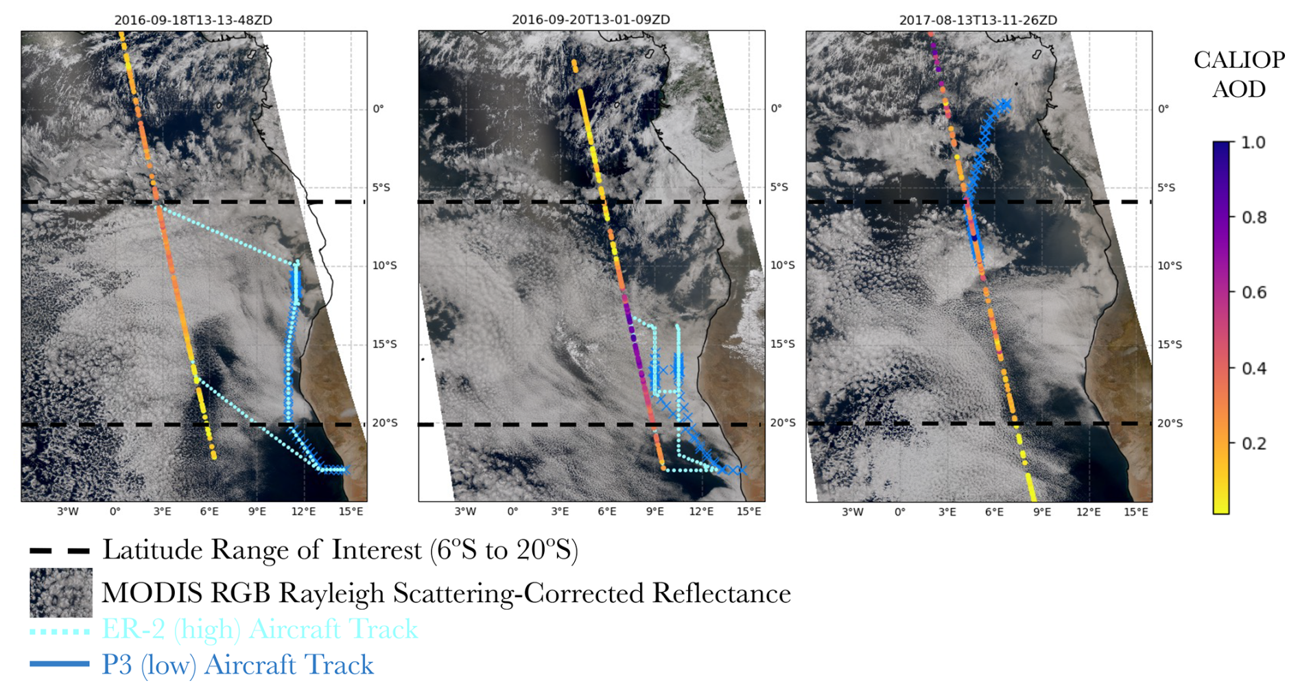
Figure 2 Three case studies during ORACLES offshore from Namibia, southern Africa, on 18 September 2016, 20 September 2016, and 13 August 2017. The color bar shows AOD across the CALIOP/ CALIPSO flight tracks. The AOD is described under version 2 in Table A3 of the Appendix. MODIS RGB Rayleigh-scattering-corrected reflectance is in the background, together with ER-2 and P3 flight tracks in light and dark blue. 18 September 2016 and 20 September 2016 show satisfying co-location with the ER-2 aircraft. 13 August 2017 shows satisfying co-location with the P3 aircraft.

Figure 3 illustrates the number of S1, S2, S3, and S4 scenarios along the tracks on all 3 days of Fig. 2 when focusing between 6 and 20° S in latitude (see dashed horizontal black line in Fig. 2). We note a dominance of aerosol above thick clouds (S1); followed by unassigned (N/A) cases; and, lastly, non-cloudy sky (S4) and aerosol above and below thick, thin, and/or broken clouds (S2 and S3).

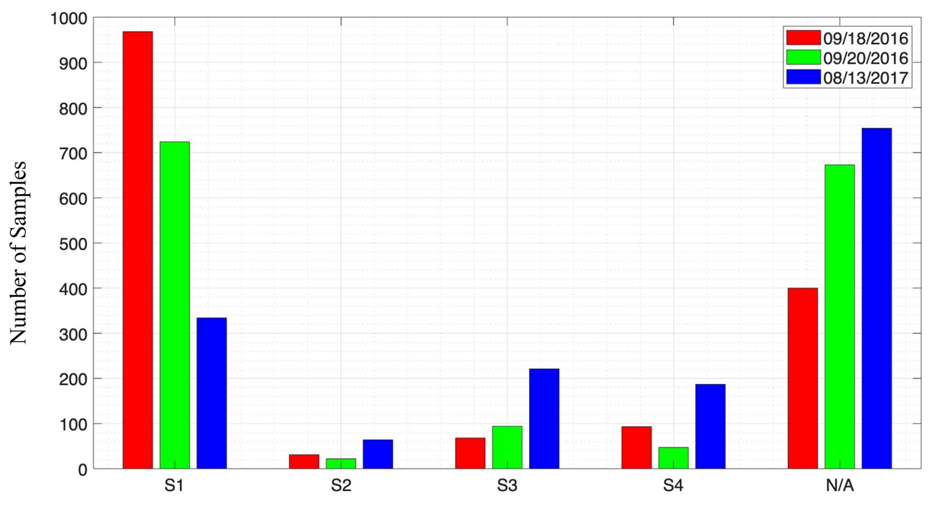
Figure 3 Number of S1–S4 samples on 18 September 2016, 20 September 2016, and 13 August 2017 (red, green, and blue) during ORACLES between 6 and 20° S in latitude (see dashed horizontal black line in Fig. 2). S1 – thick and uniform clouds with MODIS COT >4; S2 – thick, can be broken clouds, with MODIS COT >4; S3 – thin, can be broken clouds, with MODIS COT <4; and S4 – non-cloudy sky, can contain small broken clouds (MODIS cloud mask = “clear”). See Table 3 for more details on S1–S4. N/A denotes the number of cases that were not assigned a scenario S1–S4 for various reasons (see reasons for these cases in the text).

Any scenario labeled “N/A” in Fig. 3 is a scenario that is not assigned to any of the S1 through S4 cases. These “N/A” scenarios constitute 26 %, 43 %, and 48 % of the entire number of 1 km profiles on 18 September 2016, 20 September 2016, and 13 August 2017, respectively (i.e., N=400, 673, and 754 compared to N=1560 from 6 to 20° S). These scenarios could be unassigned in our study due to any of the following reasons:

1. More than one cloud is present above a 3 km altitude (e.g., cirrus clouds are present over LWLC).

2. The cloud-phase classification is unreliable (e.g., CALIOP either fails to classify the cloud as LWLC or instead successfully classifies the cloud as non-LWLC).

3. The CALIOP- and MODIS-based cloud characterization and/or non-cloudy-sky determination report conflicting results (e.g., (a) CALIOP identifies a “thick cloud” along the CALIOP track when MODIS identifies a cloud with COT <4 within the same 1 km pixel, or (b) MODIS identifies mostly cloudy sky within the 1 km pixel, whereas CALIOP profiles suggest mostly non-cloudy sky).

4. CALIOP detects cloudy sky, but MODIS does not have a valid collocated COT retrieval.

3.2 Aerosol, cloud properties, and all-sky DARE_obs

Figure 4 shows the probability distribution functions (PDFs) of the AOD above clouds (S1–S3); AOD in non-cloudy sky (S4); all-sky SSA, ASY, and EAE (S1–S4) values of the aerosol layer at the highest altitude; COT, CWP, and CER of all clouds (S1–S3); and 24 h mean DARE_obs values for all 3 days (red, green, and blue). Table 5 shows the mean values corresponding to the PDFs of Fig. 4 and other parameters, such as DARE_obs, uncertainties in DARE_obs (instant and 24 h), uncertainties in CWP, AOD, CF, ATH, and ABH. Table A6 in the Appendix complements Table 5 by providing the same parameters for scenarios S1, S2, and S3 separately.

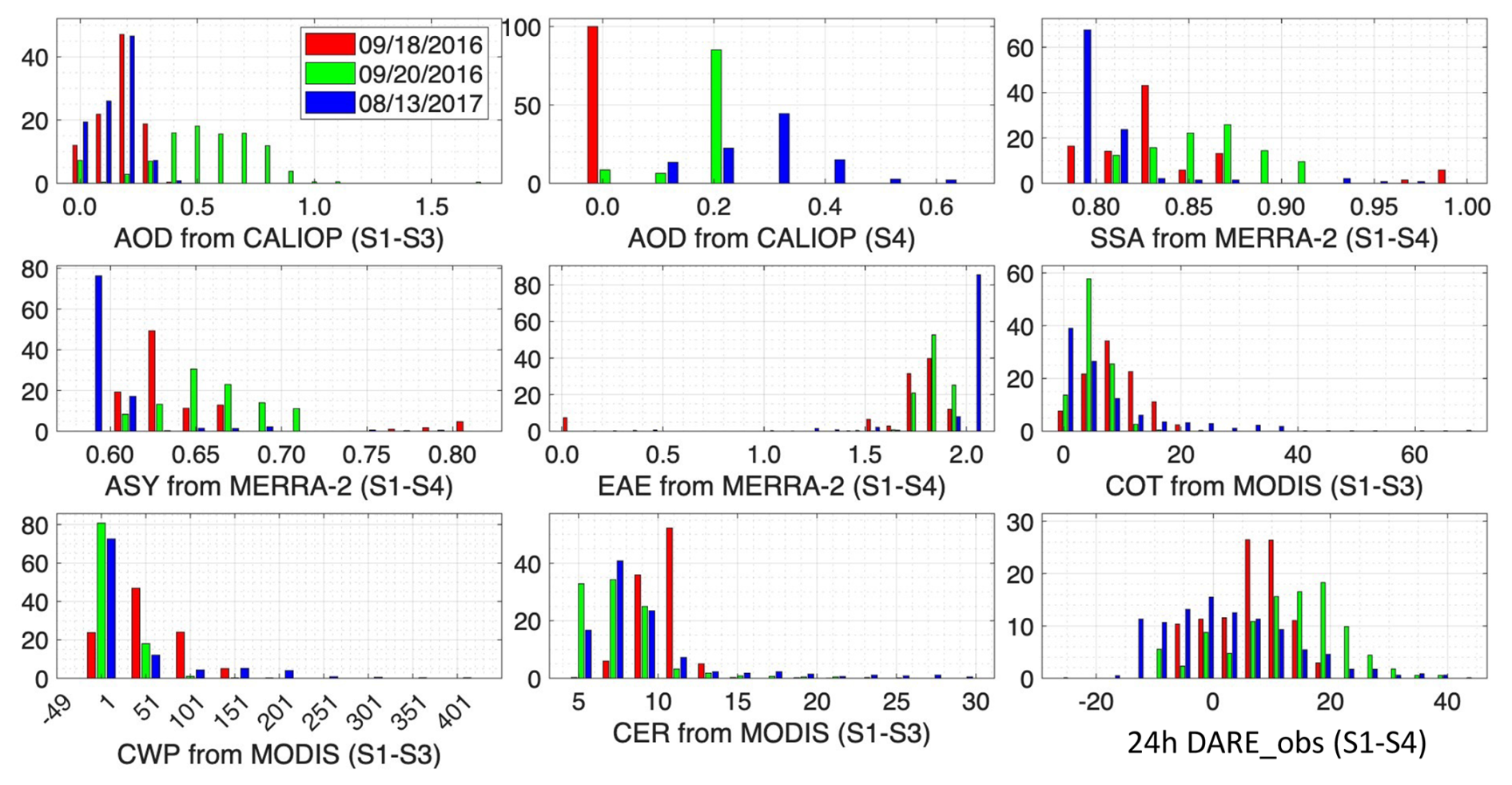
Figure 4 Probability distribution function of aerosol, cloud, and 24 h mean DARE_obs properties on 18 September 2016, 20 September 2016, and 13 August 2017 (red, green, and blue) during ORACLES. The y axis is the number of points in each bin. Table 5 shows the averaged values on each day in non-cloudy-sky, cloudy, and all-sky conditions. Cloud-retrieved optical properties are not corrected for aerosols above them. Latitudes are selected between 6 and 20° S. AOD is at 532 nm; SSA, ASY, and 24 h DARE_obs are in the 442–625 nm RRTMG channel; EAE is computed between the 442–625 nm and the 625–778 nm RRTMG channels; and SSA, EAE, and ASY are selected at the highest aerosol height in MERRA-2.

Table 5 Averaged DARE_obs values and corresponding averaged aerosol and cloud input values in the case of non-cloudy-sky (S4), cloudy (S1–S3), and all-sky (S1–S4) scenarios. The all-sky (S1–S4) averaged values correspond to the PDFs in the lower-right panel of Fig. 4. We display results corresponding to AOD version 2 (see Table A3 for more information on version 2). ΔSSA is fixed at 0.05, and ΔASY is fixed at 0.02 (see Table 4). Latitudes are selected between 6 and 20° S. See Table A6 for a breakdown of cloudy sky (S1–S3) into S1, S2, and S3 scenarios separately. AOD is at 532 nm; SSA, ASY, and 24 h DARE_obs are in the 442–625 nm RRTMG channel; EAE is computed between the 442–625 nm and the 625–778 nm RRTMG channels; and SSA, EAE, and ASY are selected at the highest aerosol height in MERRA-2.

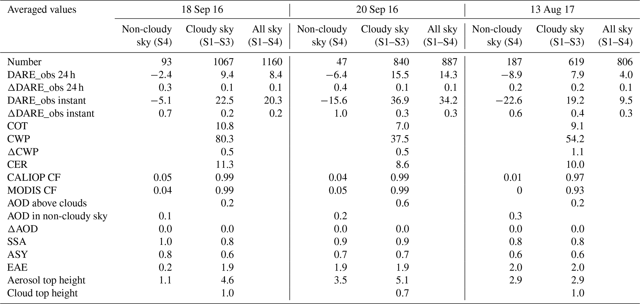
Figure 4 shows a variability of 24 h all-sky (S1–S4) DARE_obs from −25 to 40 W m⁻² on all 3 days (bottom right). It also shows that the lowest all-sky 24 h DARE_obs values are on 13 August 2017 (in blue), confirmed by a mean all-sky 24 h DARE_obs value of $\sim \mathrm{4}\pm \mathrm{0.1}$ W m⁻² on 13 August 2017 in Table 5 (compared to $\sim \mathrm{8}\pm \mathrm{0.1}$ and $\sim \mathrm{14}\pm \mathrm{0.1}$ W m⁻² on the other days). This finding can be explained by 13 August 2017 also showing the highest number of non-cloudy-sky (S4) cases in Fig. 3, the lowest mean CALIOP CF values in non-cloudy sky (indicating minimal cloud contamination of the S4 cases), and the highest mean AOD value in non-cloudy sky (i.e., 0.3 compared to 0.1–0.2 on the other days) in Table 5. The AOD above clouds on all 3 days (i.e., a mean AOD value from 0.2 to 0.6 in Table 5) agrees with monthly averages of 0.2–0.6 in September 2016 and August 2017 in Chang et al. (2023) (see their Fig. 1). Also, Doherty et al. (2022) (see their Table 3) show a monthly average of integrated vertical profiles of scattering and absorption coefficients above clouds from in situ instruments of 0.4 in 2016 and 0.3–0.6 in 2017. Mean 24 h cloudy (S1–S3) DARE_obs values are $\sim \mathrm{9}\pm \mathrm{0.1}$, 15±0.1, and 8±0.2 W m⁻² on 18 September 2016, 20 September 2016, and 13 August 2017, respectively, as shown in Table 5. These values are higher than in Kacenelenbogen et al. (2019), where we found mean 24 h cloudy DARE_obs values of 2.49±2.54 and 2.87±2.33 W m⁻² in JJA and SON over a region between 19 and 2° N and 10° W and 8° E, respectively, using satellite data from 2008 to 2012. We attribute this difference in cloudy DARE_obs to a difference in the period, the spatial domain, and the way DARE_obs is computed. Here, the highest mean 24 h cloudy (S1–S3) DARE_obs value of ∼15 W m⁻² is explained by the highest mean AOD above clouds of 0.6. Table 1 in Kacenelenbogen et al. (2019) lists other peer-reviewed calculations of cloudy DARE_obs with which our results can be compared (e.g., Chand et al., 2009; Wilcox, 2012; De Graaf et al., 2012, 2014; Meyer et al., 2013, 2015; Peers et al., 2015; Feng and Christopher, 2015).

Figure 5 illustrates the spatial evolution of key input parameters to our (instant and 24 h mean) DARE_obs calculations, together with the DARE_obs values themselves along the CALIOP track on 13 August 2017. Figures A6 and A7 in the Appendix show similar plots for the other 2 days. From the top to the bottom panels, the figures show the locations of the S1, S2, S3, and S4 cases; the AOD (above cloud and in non-cloudy sky) ±ΔAOD; COT, CER, and CWP ±ΔCWP values along the CALIOP track; and DARE_obs ±ΔDARE_obs (24 h and instant). The low 24 h DARE_obs value of ∼4 W m⁻² on 13 August 2017 (see Table 5) is in fact accompanied by strong DARE_obs variability along the track, as illustrated in Fig. 5. For example, a thick cloud is detected at ∼10° S latitude (see also Fig. 2), which corresponds to a peak in COT and CWP (but not CER) values. Over this region, our algorithm detects many S1 cases (in red), for which the AOD and SSA both remain relatively constant (i.e., a light-absorbing aerosol plume with a strong loading) and the COT values increase. This leads to a sharp increase in the DARE_obs values (i.e., more warming of the atmosphere).

Figure 5 Spatial evolution of key input parameters to our DARE_obs calculations, together with the DARE_obs values (24 h and instant) along the CALIOP track on 13 August 2017. From the top to bottom panel: (a) S1, S2, S3, and S4 cases (red, dark blue, light blue, and orange, respectively); (b) version 2 AOD ±ΔAOD at 532 nm (red above cloud and orange in non-cloudy sky); (c) COT (dark blue), CER (light blue), and CWP ±ΔCWP (magenta); and (d) 24 h (dark green) and instant (light green) DARE_obs ±ΔDARE_obs (W m⁻²) in the 442–625 nm RRTMG channel. Cloud-retrieved optical properties are not corrected for aerosols above them. Instead of showing latitudes between 60 and 20° S, we reduce the latitude range from 6 to 11° S for visibility. See Figs. A6 and A7 for the other 2 days.

Figure A8 in the Appendix illustrates 24 h DARE_obs values as a function of AOD and SSA in non-cloudy-sky conditions (i.e., S4) on the right and as a function of AOD and COT in cloudy conditions (i.e., S1–S3) on the left on 18 September 2016, 20 September 2016, and 13 August 2017. First, as expected, DARE_obs values are more and more negative when paired with increasing AOD values in non-cloudy sky and any SSA values. Second, also as expected, we observe a clear increase in positive DARE_obs values when paired with an increase in AOD values above clouds. In cloudy conditions and when the AOD above clouds remains similar, DARE_obs records consistently higher values (more warming) when paired with a larger COT value. Note that we were able to reproduce this relationship in our theoretical calculations (see Fig. A2).

3.3 Assessment of DARE_obs

3.3.1 Using DARE_param

We first assess DARE_obs using the DARE_param calculations described in Sect. 2.2 and Table 2. The DARE_param parameterization was developed during ORACLES, an airborne field campaign specifically designed to investigate aerosols above clouds. Because the DARE_param parameterization applies only to the subset of cloudy scenarios (i.e., S1–S3) measured during ORACLES, we do not include DARE_obs vs. DARE_param comparisons in non-cloudy-sky conditions (i.e., S4) in this paper. Figure 6 shows instant DARE_param on the x axis and instant DARE_obs on the y axis, colored by the AOD values above clouds on 18 September 2016 (left), 20 September 2016 (middle), and 13 August 2017 (right). The black crosses denote CALIOP cloud fractions that are below 1 (i.e., more broken clouds). The first section of Table 6 summarizes the statistics.

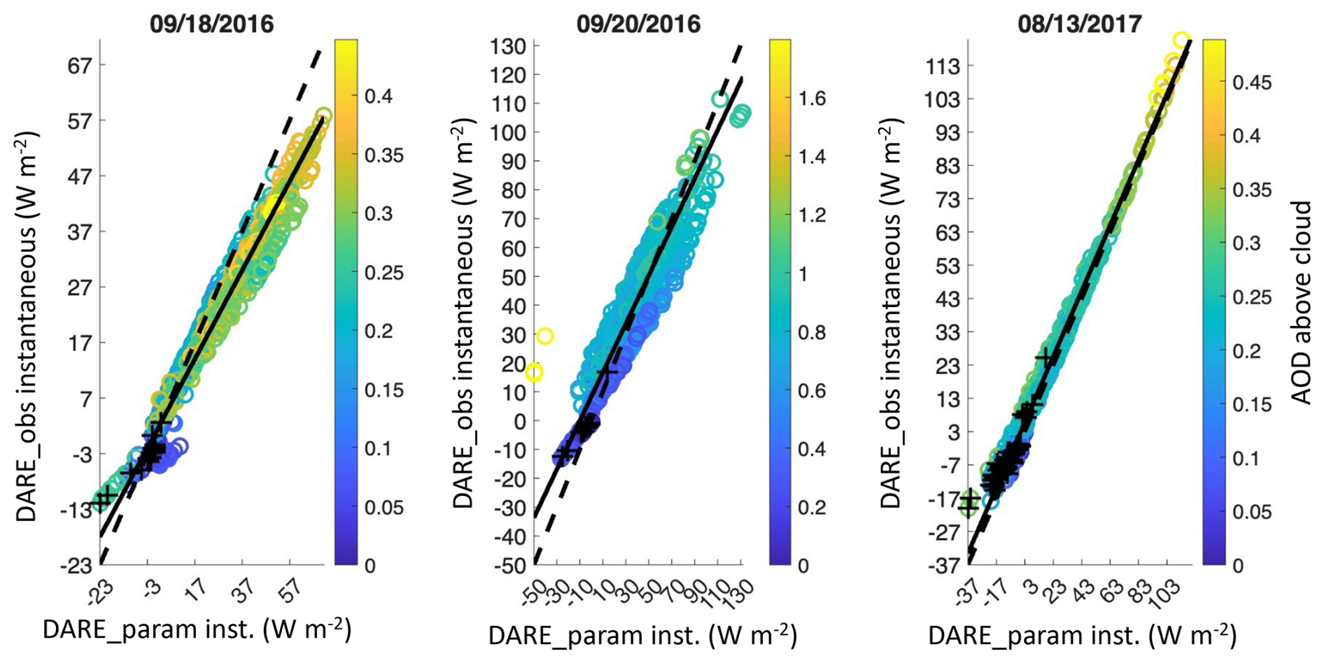
Figure 6 Semi-observational instant DARE_obs (y axis) compared to DARE_param (x axis) (W m⁻²) (see Sect. 2.2 and Table 2) for cloudy cases (i.e., S1, S2, and S3 in Table 3) at 532 nm (i.e., in the 442–625 nm channel). Cloud-retrieved optical properties are not corrected for aerosols above them. Latitudes are selected between 6 and 20° S. Black crosses show points with CALIOP cloud fraction below 1 (i.e., more broken clouds). See Table 6 for statistics.

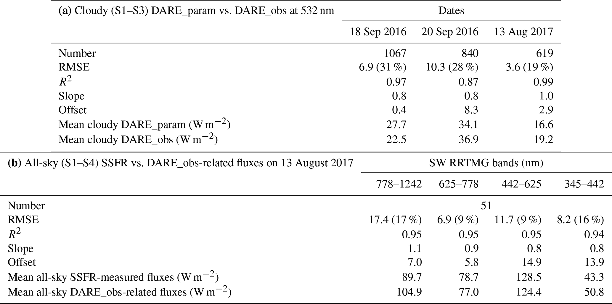
When evaluating our semi-observational DARE_obs with coincident parameterized DARE_param over all types of clouds (i.e., S1, S2, and S3 in Table 3) and for our three case studies, we find generally satisfying agreement (R²=0.87 to 0.99, slope = 0.80 to 0.99, offset = 0.37 to 8.30, N=619 to 1067 in panel a of Table 6). We posit that the slight differences between DARE_obs and DARE_param (see, for example, the mean cloudy DARE_param and DARE_obs values in panel a of Table 6) pertain to how they are computed. On the one hand, we assume MERRA-2's vertical distribution of SSA for the DARE_obs calculations, even though the SSA magnitude lies outside the observed SSA variability during ORACLES (i.e., as seen in Fig. 4b in Cochrane et al., 2021, the peak in the in situ SSA values measured at 532 nm is between 0.85 and 0.86). By invoking this assumption, we can either overestimate DARE_obs if the MERRA-2 SSA value is too low or underestimate DARE_obs if the MERRA-2 SSA value is too high. For example, when computing DARE_theo (see Fig. A2), we record lower DARE_theo values (by ∼10 W m⁻²) when adding more scattering aerosols (i.e., “continental”) to already absorbing aerosols (i.e., “urban”) over a thick cloud (COT = 10). A second example is seen on 20 September 2016, where the two data points showing high AOD values above clouds (in yellow) and causing an offset in the DARE_param vs. DARE_obs regression line (∼8 in Table 6) are likely due to an underestimation of MERRA-2 SSA, which in turn causes an overestimation of DARE_obs compared to DARE_param. On the other hand, while DARE_param is computed using the same AOD and cloud microphysical properties as DARE_obs, the DARE_param framework was developed specifically for aerosols above homogeneous cloud conditions (i.e., S1) and thus might not apply as well to broken and/or thin clouds (i.e., S2 and S3). The various amounts of S1, S2, and S3 cases during our three case studies (illustrated in Fig. 3) likely influence the DARE_param accuracy. We also note a distinctive feature in Fig. 6 on 18 September 2016 away from the 1:1 line for low AOD and CALIOP cloud fractions below 1 (black crosses). This feature is very likely due to cloud inhomogeneities paired with low AOD values.

Table 6 Number, root mean square error (RMSE), correlation coefficient (R²), and linear regression parameters between (a) cloudy (S1–S3) DARE_param vs. DARE_obs at 532 nm (i.e., in the 442–625 nm channel) for our three case studies and (b) all-sky (S1–S4) SSFR-measured and DARE_obs-related fluxes in four SW RRTMG broadband channels; % in parenthesis is based on the mean cloudy DARE_obs in panel (a) and the mean DARE_obs-related fluxes in panel (b). Latitudes are between 6 and 20° S.

3.3.2 Using airborne SSFR upward spectral irradiance measurements

After the statistical assessment of DARE_obs using DARE_param in Sect. 3.3.1, we now assess DARE_obs using the spatially and temporally co-located SSFR measurements on our third case study of 13 August 2017 (see Fig. 2). Although the collocation only provides limited samples for validation, the directly measured irradiance (which can be used to indicate radiative effects) from SSFR can provide further insights into our DARE_obs results.

We consider only those locations and times when (i) the aircraft flies above the CALIOP-inferred aerosol top height, (ii) the aircraft measurements are within (≤) 0.7 km, (iii) the aircraft measurements are within ±30 min of the CALIOP observations (i.e., between 13:00 and 14:00 UTC as the overpass occurs at ∼13:30 UTC over the region), and (iv) the aircraft is leveled (i.e., the aircraft pitch and role are both within ±5°). After applying those filters, we find N=51 valid (>0) paired CALIOP–SSFR flux results corresponding to aircraft altitudes between 3.57 and 6.46 km above CALIOP aerosol top heights between 3.05 and 3.14 km, distances between CALIOP and the nearest SSFR measurements from 0.44 to 0.70 km, times of SSFR measurements between 13:14 and 13:55 UTC, joint latitudes between 7.86 and 9.56° S (see Fig. 2 for context), and aircraft pitch and role between −1.5 and 3.5°. We use SSFR files called “20170813_calibspecs_20171106p_1324_20170814s_150C_attcorr_ratio.nc” and “20170813_librad_info.nc”.

As a reminder, DARE_obs is the subtraction of the upward spectral broadband irradiances (or fluxes received by a surface per unit area), $F_{\mathrm{b}\mathit{\lambda }\mathrm{no}\mathrm{aerosol}}^{\uparrow }-F_{\mathrm{b}\mathit{\lambda }\mathrm{aerosols}}^{\uparrow }$, in 13 RRTMG broadband channels (from 200 to 3846 nm, with spectral bands ranging from 56 to 769 nm in W m⁻²). The airborne SSFR instrument mounted on the bottom of the aircraft measured the upward flux, $F_{\mathit{\lambda }}^{\uparrow }$, in narrow spectral bands (from 350 to 2200 nm, with a spectral resolution of 6 to 12 nm in W m⁻² nm⁻¹). We spectrally integrate SSFR $F_{\mathit{\lambda }}^{\uparrow }$ within each SW RRTMG broadband channel using a trapezoidal numerical integration. For example, the first RRTMG channel that contains SSFR measurements is between 345 and 442 nm. SSFR's shortest channel is at 350 nm and measures 15 increments of 6 nm spaced $F_{\mathit{\lambda }}^{\uparrow }$ up to 442 nm, i.e., within the first RRTMG channel. Therefore, we sum all 15 increments of $F_{\mathit{\lambda }}^{\uparrow }$ from SSFR (i.e., from 350 to 442 nm) and compare this value to $F_{\mathrm{b}\mathit{\lambda }}^{\uparrow }$ in the first RRTMG channel (i.e., from 345 to 442 nm). The second part of Table 6 shows satisfying agreement between SSFR $F_{\mathit{\lambda }}^{\uparrow }$ and $F_{\mathit{\lambda }}^{\uparrow }$ at the source of our semi-observational DARE_obs in four relevant RRTMG broadband channels (i.e., 345–442, 442–625, 625–778, and 778–1242 nm). This is illustrated by a high correlation coefficient (0.94–0.95) and an RMSE value between 9 % and 17 % in Table 6. Figure A9 in the Appendix shows the comparison between SSFR-measured and DARE_obs-related fluxes as a function of distance between the aircraft and the satellite track. Figure 7 is like Fig. 5 but focuses on the comparison between collocated airborne and satellite observations (i.e., from −9.6 to −7.9° latitude). Panel (a) shows the N=51 collocated cases with valid satellite and airborne data (black crosses) and the different S1–S4 scenarios as a function of latitude. Among our N=51 points, we find a majority of S1 cases, followed by S3 and S4 cases in this stretch. Panel (b) shows AOD ±ΔAOD above clouds and in non-cloudy sky. Panel (c) shows COT, CER, and CWP ±ΔCWP. Panel (d) shows the satellite radiative fluxes, $F_{\mathrm{b}\mathit{\lambda }}^{\uparrow }$, behind our DARE_obs calculations in light green (W m⁻²) and the distance between the aircraft and the CALIOP ground track in magenta from 0.45 to 0.70 km. Panel (e) shows the absolute difference between SSFR and satellite $F_{\mathrm{b}\mathit{\lambda }}^{\uparrow }$ as a percentage of the satellite radiative fluxes in all four broadband channels (778–1242 in solid grey, 625–778 in solid black, 442–625 in dotted black, 345–442 nm in dotted grey).

From ∼9.2 to 7.9° S in latitude in Fig. 7, distances between the aircraft and the CALIOP ground track are higher (>600 m in magenta in panel d), clouds are thinner (i.e., low COT values in dark blue in panel c) and/or more broken (i.e., more S3 cases in panel a), and AOD above cloud is smaller (in red in panel b). These conditions all seem to lead to more unstable and generally higher satellite–SSFR flux differences (panel e). This is confirmed by Fig. A9, where we observe more scatter between SSFR $F_{\mathit{\lambda }}^{\uparrow }$ and $F_{\mathit{\lambda }}^{\uparrow }$ at the source of our semi-observational DARE_obs when the distance between the satellite and aircraft increases (see yellow markers) in all four channels. For increased visibility and because the spatial satellite–aircraft co-location is deteriorated from ∼9.2 to 7.9° S in latitude (and hence the data are of lesser significance to the overall analysis), we allow a few data points in panel (e) to extend beyond the figure's axes.

If we focus on points of close satellite–aircraft collocation (i.e., from ∼9.6 to 9.2° S, <600 m in magenta in panel d), satellite $F_{\mathrm{b}\mathit{\lambda }}^{\uparrow }$ (in light green in panel d) shows high values (>100 W m⁻²) due to the presence of S1 cases (red dots in panel a), high AOD in panel (b), and high COT values in panel (c). For these points, we find an absolute difference in all four broadband channels below ∼20 % and an absolute difference below 15 % between 778 and 442 nm (solid black and dotted black in panel e).

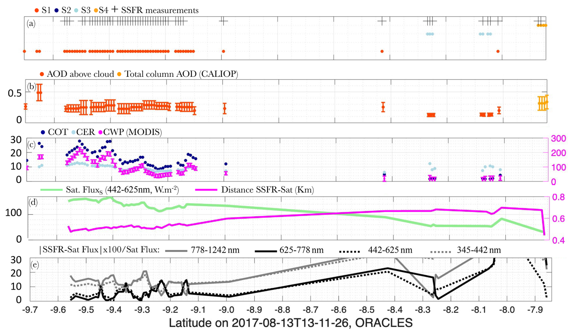
Figure 7 Spatial evolution of key input parameters along the CALIOP track, with a focus on when and where we have collocated airborne SFFR measurements for validation on 13 August 2017. From the top to the bottom panel: (a) S1, S2, S3, and S4 cases (red, dark blue, light blue, and orange, respectively) and collocated SSFR measurements (black crosses); (b) version 2 AOD ±ΔAOD at 532 nm (red above cloud and orange in non-cloudy sky); (c) COT (dark blue), CER (light blue), and CWP ±ΔCWP (magenta); (d) collocated satellite broadband (spectrally integrated) upward irradiance (or flux) received by a surface per unit area in W m⁻², $F_{\mathrm{b}\mathit{\lambda }}^{\uparrow }$, behind our DARE_obs calculations in the 442–625 nm RRTMG channel in light green (W m⁻²) and distance between the aircraft and the CALIOP ground track (km) in magenta; and (e) absolute difference between SSFR and satellite $F_{\mathrm{b}\mathit{\lambda }}^{\uparrow }$ in all four broadband channels (solid grey for 778–1242, solid black for 625–778, dotted black for 442–625, and dotted grey for 345–442 nm) as a percentage of satellite $F_{\mathrm{b}\mathit{\lambda }}^{\uparrow }$. Cloud-retrieved optical properties are not corrected for aerosols above them.

4 Discussions and future work

As described in Table 2, MERRA-2 is used in this paper to define the uppermost aerosol top height and lowermost aerosol base height below clouds, vertical distribution of the spectral aerosol extinction coefficient, vertical distribution of the spectral ASY, vertical distribution of the spectral SSA, atmospheric composition, weather, and ocean surface winds First, we currently use MERRA-2's vertical distribution of aerosols at face value with no consideration of a very likely bias in the modeled aerosol vertical profile (see Sect. 2.1.2). An improvement worth exploring would be to select the MERRA-2 vertical location that corresponds to the strongest aerosol signal. Second, another improvement would be to infer aerosol vertical distribution and loading below clouds as a function of nearby satellite-observed non-cloudy-sky aerosol cases. Third, pairing ESA/JAXA EarthCARE (Wehr et al., 2023), launched in May 2024, and NASA PACE (Werdell et al., 2019), SPEXone (Hasekamp et al., 2019), and HARP2 (Gao et al., 2023), launched in February 2024, might provide some insight into the observed vertical distribution of the spectral aerosol extinction coefficients, ASY and SSA. The EarthCARE processing chain includes operational synergistic lidar, radar, and imager cloud fields; profiles of aerosols; atmospheric heating rates; and top-of-atmosphere SW and longwave fluxes using 3D radiative transfer. These fluxes are automatically compared with EarthCARE broadband radiometer measurements, allowing for a radiative closure assessment of the retrieved cloud and aerosol properties. However, the PACE and EarthCARE satellites are never perfectly co-located in both time and space. The Atmosphere Observing System (AOS) mission, on the other hand, holds promising new science as it consists, at the time of writing, of a suite of lidar, radar, and radiometer satellites flying in formation to jointly observe aerosols, clouds, convection, and precipitation. We note that using EarthCARE's joint lidar and imager (possibly paired with PACE polarimeters) will likely reduce the number of unassigned scenarios in this paper as it will provide improved LWLC classification and optical properties and possibly reduce the mismatch between cloudy and non-cloudy-sky scenes.

In this paper, to compute our 24 h DARE_obs, we solely vary SZAs every hour during the day, which implicitly assumes constant aerosol and cloud vertical optical properties (see Table 2). On a global scale, most of the 24 h DARE variability is due to the varying solar zenith angles. Global 24 h mean DARE do not need many hourly measurements if the AOD is representative of the daily mean (e.g., at the Aqua and Terra overpass times). For example, Arola et al. (2013) found that the impact of diurnal AOD variability on the 24 h mean DARE estimates is small when averaged over all global Aerosol Robotic Network (AERONET) sites (Holben et al., 1998). Regional DARE, unlike global DARE, can show considerable variability throughout the day due to varying aerosol and cloud fields. Xu et al. (2016), for example, show that the daily mean non-cloudy-sky TOA DARE is overestimated by up to 3.9 W m⁻² in the summertime in Beijing if they use a constant Aqua MODIS AOD value, compared to accounting for the observed hourly averaged daily variability. According to Min and Zhang (2014) (see their Table 2), assuming a constant CF derived from Aqua MODIS generally leads to an underestimation (less positive) by 16 % in the all-sky DARE calculations. Chang et al. (2025) find that including the observed cloud diurnal cycle from geostationary (GEO) satellites over the southeast Atlantic results in nearly a 2-fold (about 1.4 W m⁻²) increase in the regional mean aerosol radiative warming compared to assuming a constant early-afternoon cloud field throughout the entire day. We plan on adding diurnal aerosol and cloud information in future DARE_obs calculations (instead of only varying SZA) using co-located GEO satellite observations. We note that aerosol and cloud retrievals from GEO satellites are in an earlier stage of development and less well-validated compared to their low-Earth orbit (LEO) satellite counterparts. GEO aerosol and cloud retrievals are also currently often tied to specific GEO imagers and are thus less global than their LEO counterparts. GEO AOD generally shows good agreement with ground-based AERONET AOD (e.g., low RMSE (0.12–0.17) in the case of the GEO Ocean Color Imager (GOCI) AOD over eastern Asia in Choi et al., 2019) but has unique bias patterns related to the surface-reflectance assumptions in their retrieval algorithms (e.g., negative bias of 0.04 in GOCI AOD in Choi et al., 2019). Recent improvements in algorithms consist of correcting surface reflectance, cloud masking, and/or fusing data from LEO and GEO imagers (e.g., Su et al., 2020; Zhang et al., 2020; Kim et al., 2020; Choi et al., 2019). In some cases, GEO AOD, although often biased, was shown to reproduce the AERONET AOD diurnal cycle (e.g., over Asia, on a daily average, GOCI AOD shows a diurnal variation of +20 % to −30 % in inland sites according to Lennartson et al., 2018).

Another extension to this work is to add an atmospheric scenario for which we observe one or more clouds overlying the LWLCs. With the addition of this multi-cloud atmospheric scenario, DARE_obs will be one step closer to a truly all-sky TOA SW DARE_obs. We envision this additional scenario to use (i) the CALIPSO–CloudSat–CERES–MODIS (CCCM or C3M)-derived (Kato et al., 2010, 2011) cloud height and cloud microphysical properties or equivalent EarthCARE-derived product (e.g., as in Table 1 of Mason et al., 2024) and (ii) MERRA-2-simulated aerosol extensive and intensive properties. The new all-sky DARE_obs results can then be evaluated using collocated airborne field campaign observations such as from the HSRL-2 and the SFFR instruments during the Cloud, Aerosol and Monsoon Processes Philippines Experiment (CAMP²Ex) in 2019 over southeast Asia. Note that adding atmospheric scenes showing multiple clouds on the vertical would increase the overall number of assigned atmospheric scenarios in our study.

At present, the order of importance of key aerosol, cloud, and surface parameters in DARE calculations remains unclear. Thorsen et al. (2020) find that in non-cloudy sky, AOD, SSA, and ASY are the key aerosol parameters in order of importance for DARE calculations. However, priorities can differ regionally according to airborne DARE sensitivity studies (e.g., Cochrane et al., 2019, 2021). According to Elsey et al. (2024), the AOD uncertainty is the main contributor to the overall uncertainty in DARE, except over bright surfaces where SSA contributes the most uncertainty. We plan to apply our DARE_obs calculations to multiple years of combined satellite and model data over different regions of the world. The most important factors influencing the transferability of our method to regions of the globe outside the southeast Atlantic are (i) different Earth surfaces (i.e., ocean vs. different land types) and (ii) different horizontal, vertical, and temporal distributions of aerosol and cloud types and amounts. Our method requires aerosols in cloud-free skies and above and below single thick, thin, and/or broken low warm liquid clouds. Kacenelenbogen et al. (2019) define six major global aerosol “hotspots” over single thick low warm liquid clouds (i.e., different aerosol regimes above the same type of clouds) in the northeast Pacific, the southeast Pacific, the tropical Atlantic, the southeast Atlantic, the Indian Ocean, offshore from western Australia, and the northwest Pacific (see their Fig. 6 and Table 2 for a list of studies over these regions). According to Fig. 7d of Kacenelenbogen et al. (2019), the region of the southeast Atlantic (this paper) shows the highest mean annual percentage of high AOD values above clouds compared to the other five regions. Note that we also plan to apply our DARE_obs calculations to regions that show different cloud regimes in addition to different aerosol regimes (e.g., the southeast Atlantic; the tropical Atlantic; and a region encompassing the latter two, representing the transition between these two regimes). We then plan to use this larger DARE_obs dataset for different atmospheric scenarios, over specific regions of the world and linked to key cloud, aerosol, and surface input parameters to assess the order of importance of these parameters in DARE_obs calculations for specific aerosol and cloud regimes.

5 Conclusion

We compute TOA SW all-sky DARE_obs combining CALIOP, MODIS, and MERRA-2 along the CALIOP track. These computations are made for four different atmospheric scenarios of aerosols above and below thick, thin, and/or broken clouds or aerosols in (mostly) non-cloudy skies. The clouds in our study must be single-layer and low-level (<3 km) liquid clouds. We focus our analysis on 3 days over the southeast Atlantic, for which we compare our semi-observational DARE_obs results to co-located suborbital aerosol and cloud observations during the ORACLES field campaign. During these 3 days, satellite observations show a high number of cases, with aerosols above and below thick and homogeneous clouds (i.e., N=334–968 or 21 %–62 % of our dataset), followed by cases that are not assigned in our study (i.e., N=400–754 or 26 %–48 % of our dataset).

The semi-observational 24 h average DARE_obs values for our 3 day range from −25 (cooling) to 40 W m⁻² (warming). Highly positive DARE_obs values are mostly due to aerosols with high AOD above clouds with high COT values. Highly negative DARE_obs values, on the other hand, are mostly due to aerosols with high AOD values in non-cloudy-sky cases. We use two ways of evaluating our semi-observational DARE_obs: (1) a DARE_param parameterization, dependent on the AOD and cloud albedo, which was designed using SSFR measurements during the ORACLES field campaign, and (2) an upward irradiance (or flux) directly measured by the airborne SSFR instrument. First, we demonstrate agreement between our semi-observational satellite DARE_obs and coincident parameterized DARE_param over the region (R²=0.97–0.99, RMSE = 19 %–31 %, N=619–1067). Second, we also demonstrate agreement between our semi-observational satellite upward spectral irradiance with coincident measurements from the co-located SSFR instrument in four shortwave broadband channels during ORACLES (R²=0.94–0.95, RMSE = 9 %–17 %, N=51).

We emphasize that using the EarthCARE lidar and imager instruments instead of pairing A-Train's CALIOP and MODIS, as well as adding cases with one or more clouds above our single water cloud, would bring our results closer to truly all-sky DARE results (and drastically decrease the number of unassigned atmospheric scenarios in our study). We also plan on adding aerosol and cloud diurnal cycle information from co-located geostationary satellites to improve our diurnal mean all-sky semi-observational DARE_obs results. Finally, in this paper, we have concentrated on three case studies to examine our methodology in detail and evaluate the results against airborne SSFR measurements. This is a necessary first step before applying our algorithm to multiple years of combined satellite and model data over different regions of the world. Our goal is to ultimately assess the order of importance of atmospheric parameters in the calculation of DARE_obs for specific aerosol and cloud regimes. Expanding on the work done in this study will inform future missions on where, when, and how accurately the retrievals should be performed to most effectively reduce all-sky DARE uncertainties.

Appendix A

A1 Data and method

Table A1 Theoretical DARE_theo calculations for aerosols above clouds in our study and their respective inputs. n/a: not applicable.

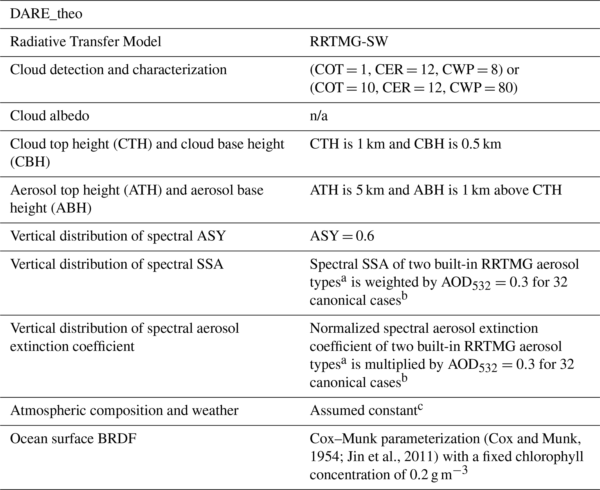
^a See “continental average” and “urban” aerosol types in Fig. A1; ^b see upper panels (a, b, c, d) in Fig. A2; ^c CO₂, N₂O, CH₄, O₂, and ocean surface wind speed are assumed to be equal to a single value (i.e., 400 ppmv, 0.3 ppmv, 1.7 ppmv, 0.0 kg m⁻³, and 4 m s⁻¹, respectively); and the pressure, temperature, air density, water vapor, and ozone profiles are also assumed constant and illustrated in Table A2. The instant DARE_theo uses the solar zenith angle (SZA) at 15° S latitude and 8° E longitude on 15 September 2016. We compute 24 instant DARE_theo values based on 24 SZAs (every hour) throughout the day (at the same location and date) and average all instant DARE_theo to obtain the 24 h DARE_theo values.

Table A2 Atmospheric profiles of pressure, temperature, air density, water vapor, and ozone used in the calculation of DARE_theo (see Table A1); see the legend of Table A1 for constant CO₂, N₂O, CH₄, O₂, and ocean surface wind speed values.

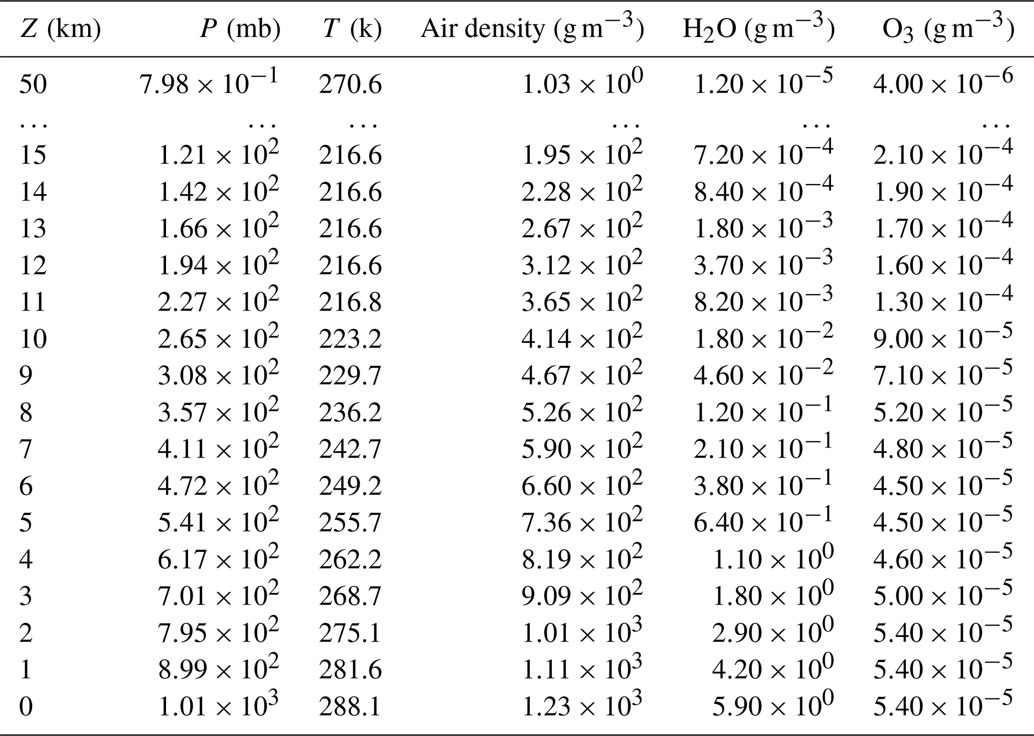
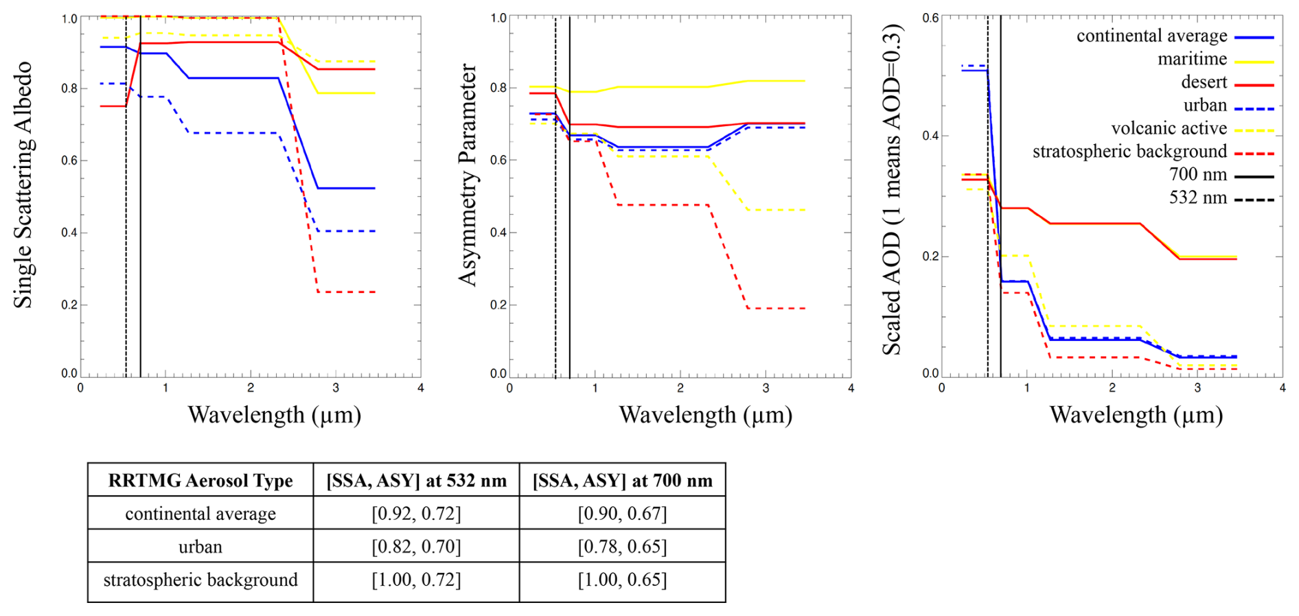
Figure A1 RRTMG “built-in” aerosol types used in the calculation of DARE_theo (see Table A1). SSA is 0.92 (0.90), 0.82 (0.78), and 1.00 (1.00) for RRTMG “continental average”, “urban”, and “stratospheric background” aerosol types at 532 (700) nm. Note that RRTMG “continental average” seems to correspond roughly to biomass burning smoke aerosol types in Russell et al. (2014). Also note that RRTMG “urban” seems to correspond to aerosols with considerably higher light absorption properties than those of the smoke types in Russell et al. (2014). ASY is 0.72 (0.67), 0.70 (0.65), and 0.72 (0.65) for RRTMG “continental average”, “urban”, and “stratospheric background” at 532 (700) nm. Aerosol types are taken from the Optical Properties of Aerosols and Clouds (OPAC) software (Hess et al., 1998).

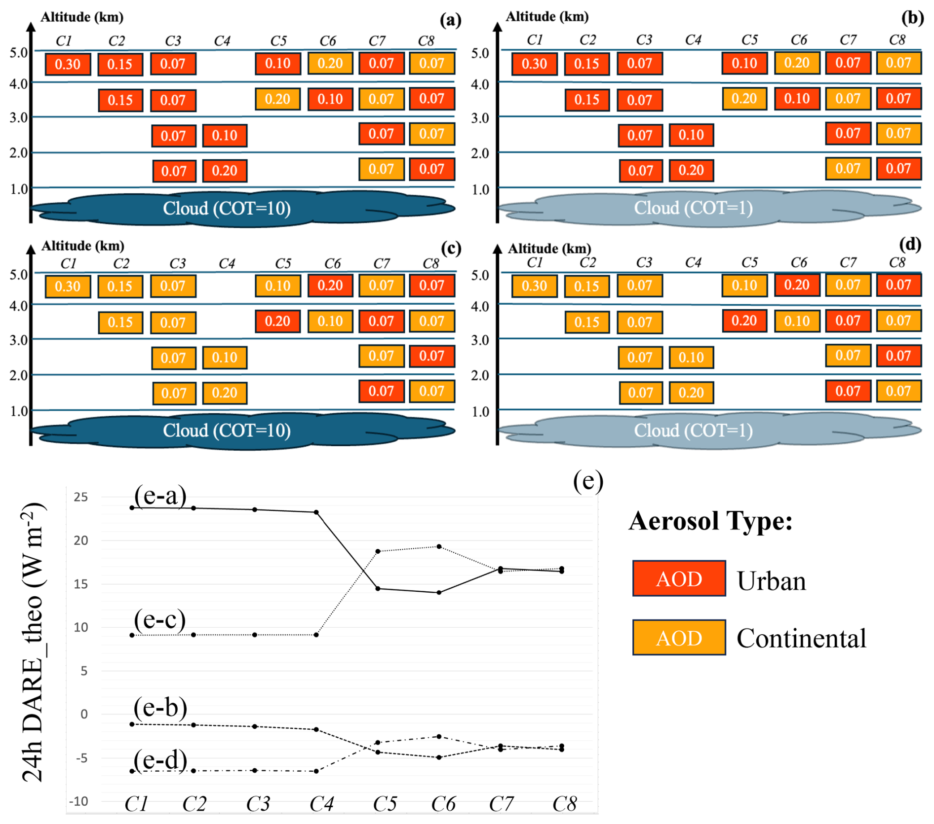
Figure A2 The 24 h mean theoretical DARE_theo (in W m⁻²) results in (e) for 32 canonical cases (i.e., eight cases in a–d), where we vary COT, the number of aerosol layers over clouds, the order of aerosol types, and the loading of aerosols over clouds. Orange and red boxes depict two “built-in” RRTMG aerosol types, with “continental average” in orange and “urban” in red; see Fig. A1 for the optical and microphysical properties of these aerosol types. The vertical distribution of spectral SSA and extinction coefficient are weighted by the AOD above clouds that is assumed constant and equal to 0.3 at 532 nm (i.e., in the 442–625 nm RRTMG broadband channel). See Table A1 for a list of the inputs to the DARE_theo calculations.

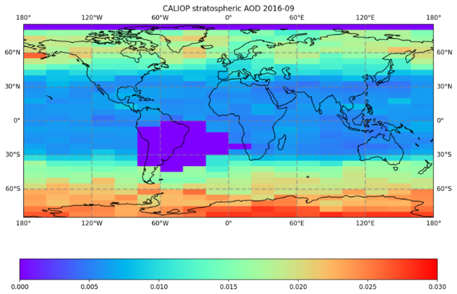
Figure A3 Stratospheric aerosols that are deleted when computing DARE_obs (see Table 2).

Table A3 Detailed description of aerosol and cloud property inputs to DARE_obs calculations for each atmospheric scenario (see Table 3 for S1–S4). We also provide more information on CALIOP-derived input aerosol parameters and describe three CALIOP-derived AOD versions. (E-1) through (E-6) denote effects of varying factors in the calculation of DARE_obs. (E-1) through (E-6) are quantified in Table A4 and reported in Sect. 2.1.4. In the main sections of this paper, we choose to display DARE_obs results with a threshold applied on the extinction coefficients (E-1), aerosols below clouds using MERRA-2 (E-2), ATH extended (E-3), CALIOP-inferred AOD version 2, and cloud properties from MODIS uncorrected for aerosols above them (E-6). n/a: not applicable.

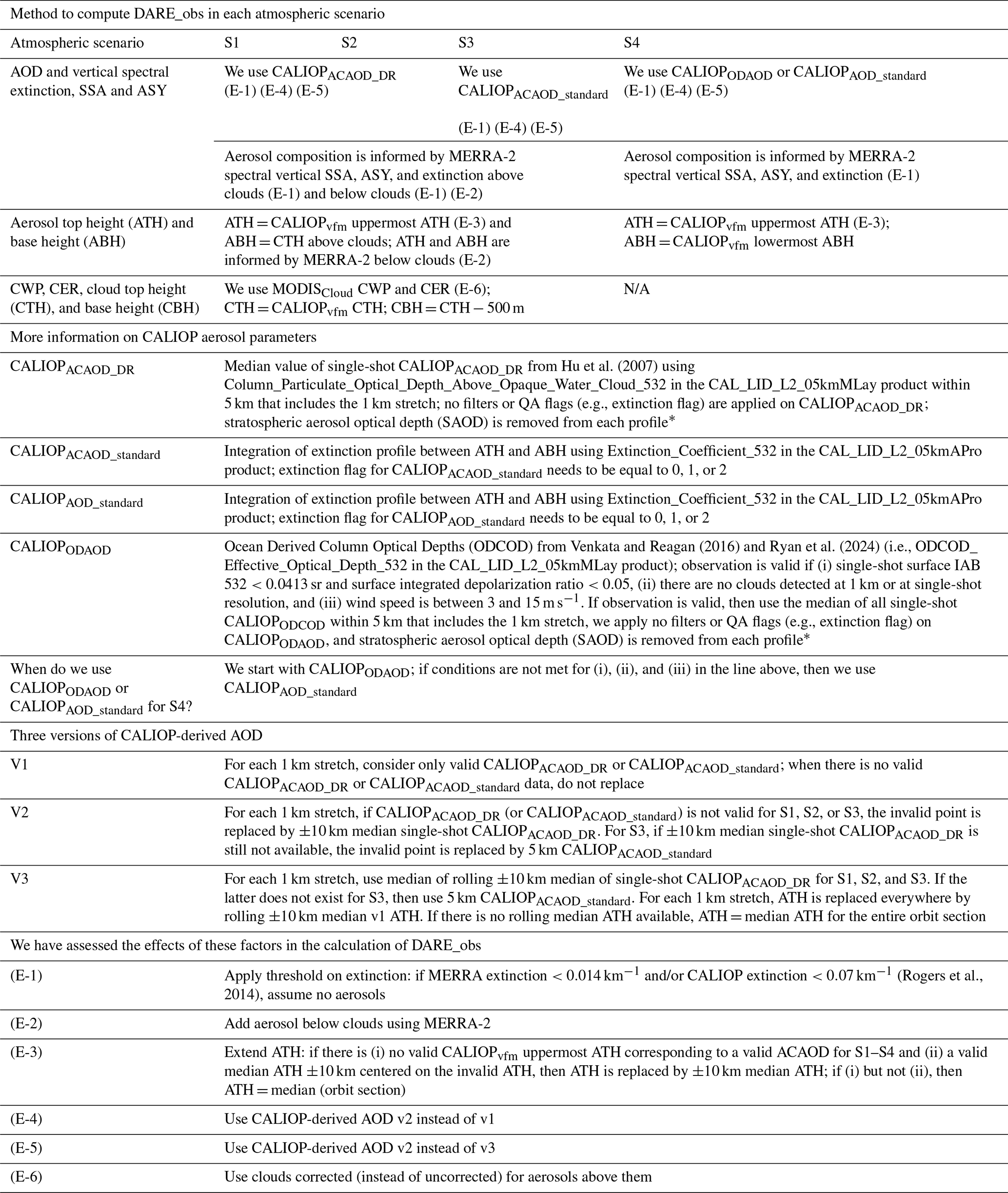
^∗ The way the stratospheric aerosol optical depth (SAOD) is removed from each profile is that we compute a zonal SAOD from the equal-angle data product (see Fig. A3), then interpolate the zonal data to the latitude grid of the CALIPSO granule observations, and remove the SAOD from either CALIOP_{ACAOD_DR} or CALIOP_ODAOD.

Table A4 Effects of (E-1) adding a lower threshold on CALIOP and MERRA-2 extinction coefficients, (E-2) adding MERRA-2 aerosol below clouds, (E-3) extending aerosol top height (ATH) when there is no valid ATH from the CALIOP standard product, (E-4) using AOD v2 instead of v1, (E-5) using AOD v3 instead of v2, and (E-6) using clouds corrected for aerosol above when AOD >0.3. Latitudes are selected between 6 and 20° S.

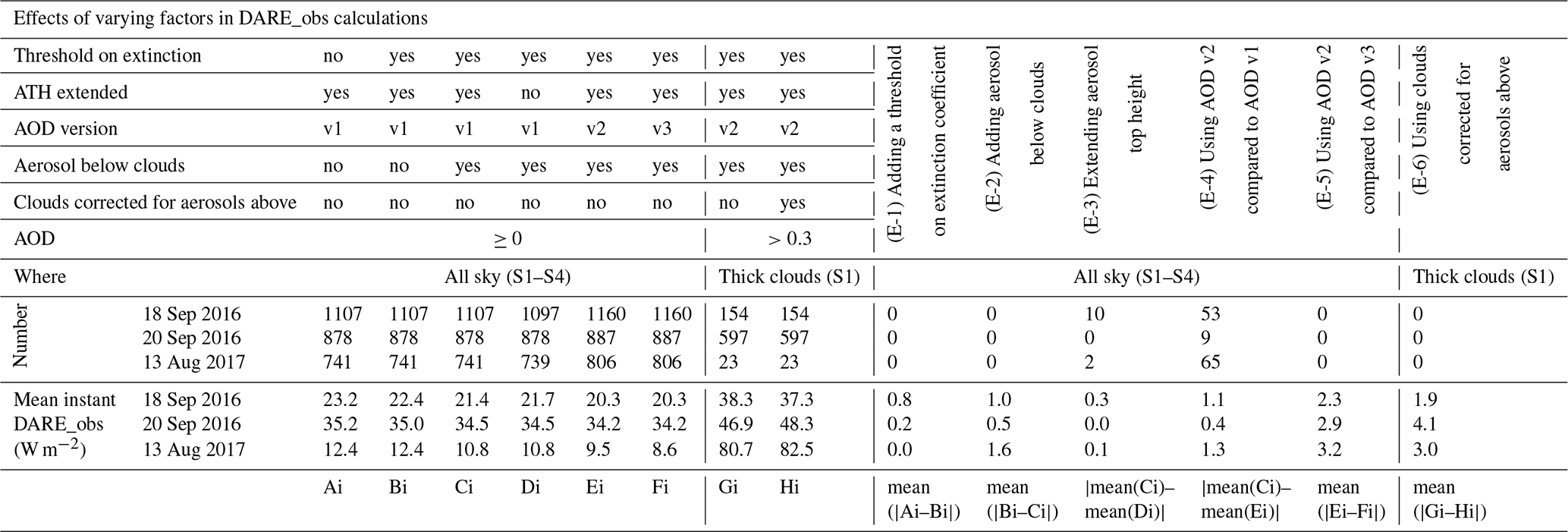
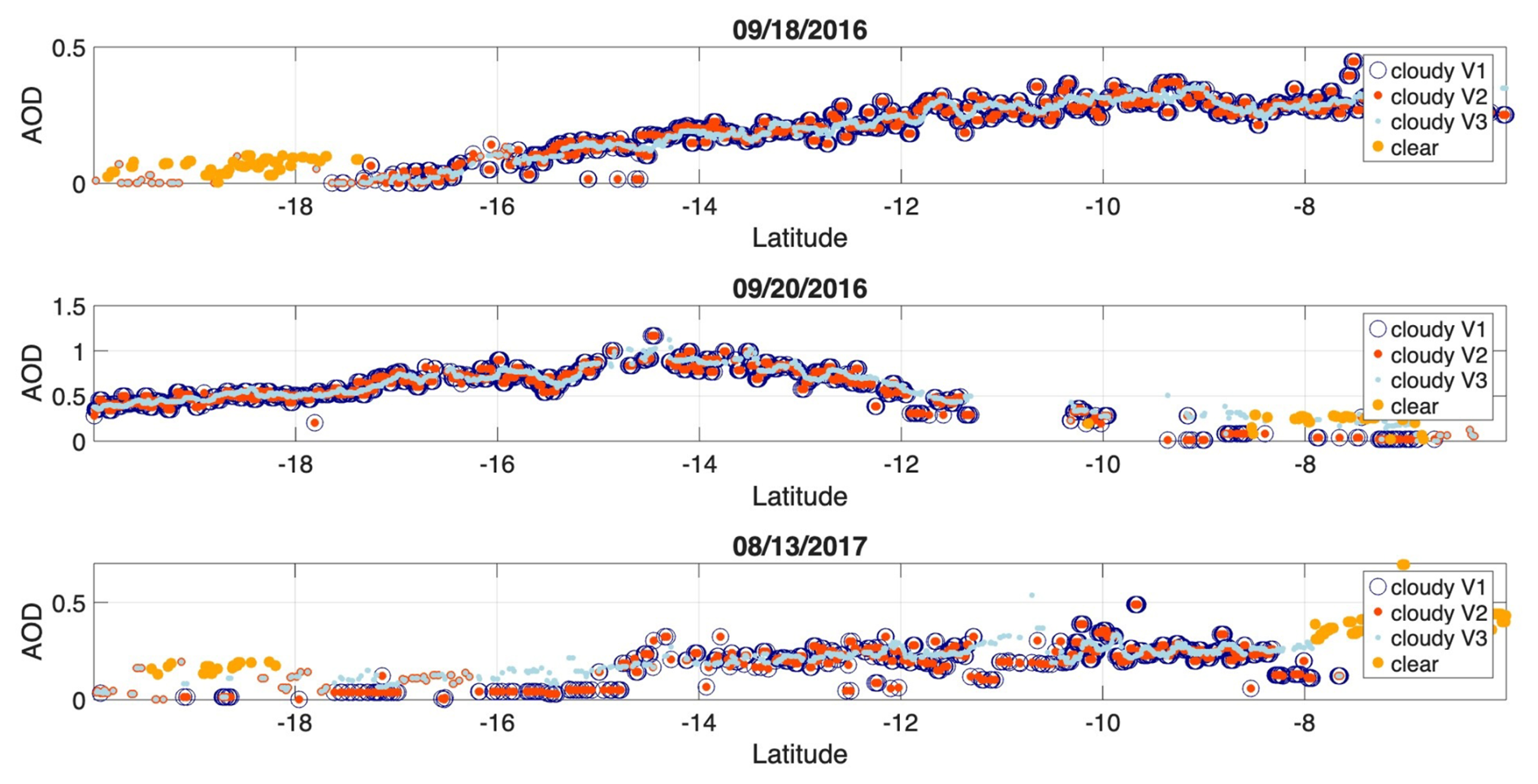
Figure A4 Evolution of CALIOP-inferred AOD v1, v2, and v3 above clouds (S1–S3) (see Table A3 for a definition of these versions) and in non-cloudy sky (S4) for our three case studies. We eventually select AOD v2 in this paper. Latitudes are selected between 6 and 20° S.

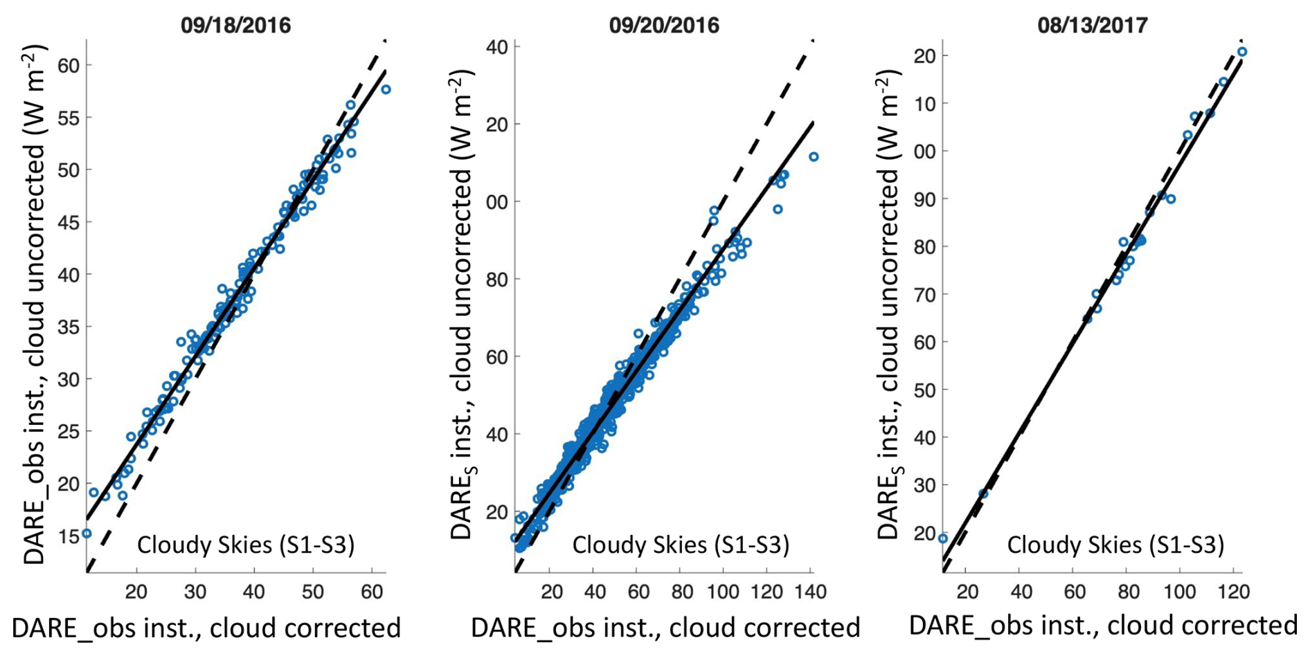
Figure A5 Illustration of the effects of using cloud properties corrected for aerosols above them in DARE_obs calculations (see E-6 in Tables A3 and A4). Semi-observational instant cloudy (S1–S3) DARE_obs (W m⁻²) (see Table 2) using MODIS COT corrected for aerosol above (x axis) vs. MODIS COT uncorrected for aerosol above (y axis). We show only values with AOD >0.3 above clouds. See Table A5 for linear regression and correlation statistics. Latitudes are selected between 6° N and 20° S.

Table A5 Effects of using cloud properties corrected for aerosols above them in DARE_obs calculations (E-6). These are the statistics behind Fig. A5, i.e., a comparison between instant DARE_obs using COT (or simply COT) with clouds corrected vs. clouds uncorrected for aerosol above them.

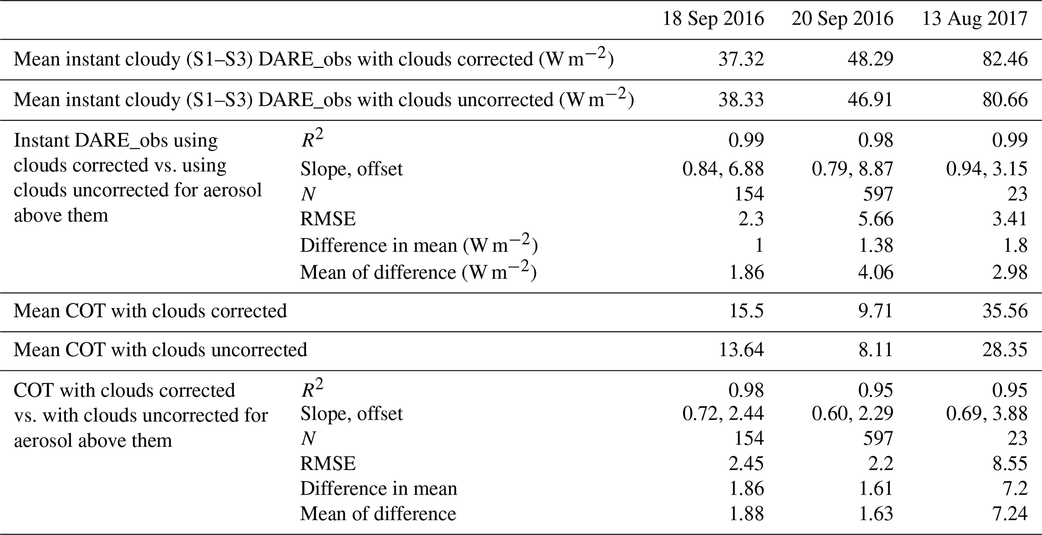
A2 Results

Table A6 This table complements Table 5 – it is a breakdown of cloudy sky (S1–S3) into individual S1, S2, and S3 scenarios (see Table 3). Averaged aerosol, cloud, and DARE_obs properties per atmospheric scenario and case study. We display results corresponding to AOD version 2 (see Table A3 for more information on version 2). ΔSSA is fixed at 0.05, and ΔASY is fixed at 0.02 (see Table 4). Latitudes are selected between 6 and 20° S. AOD is at 532 nm; SSA, ASY, and 24h DARE_obs are in the 442–625 nm RRTMG channel; EAE is computed between the 442–625 nm and the 625–778 nm RRTMG channels; and SSA, EAE, and ASY are selected at the highest aerosol height in MERRA-2.

Figure A6 Same legend as for Fig. 5 but for 18 September 2016.

Figure A7 Same legend as for Fig. 5 but for 20 September 2016.

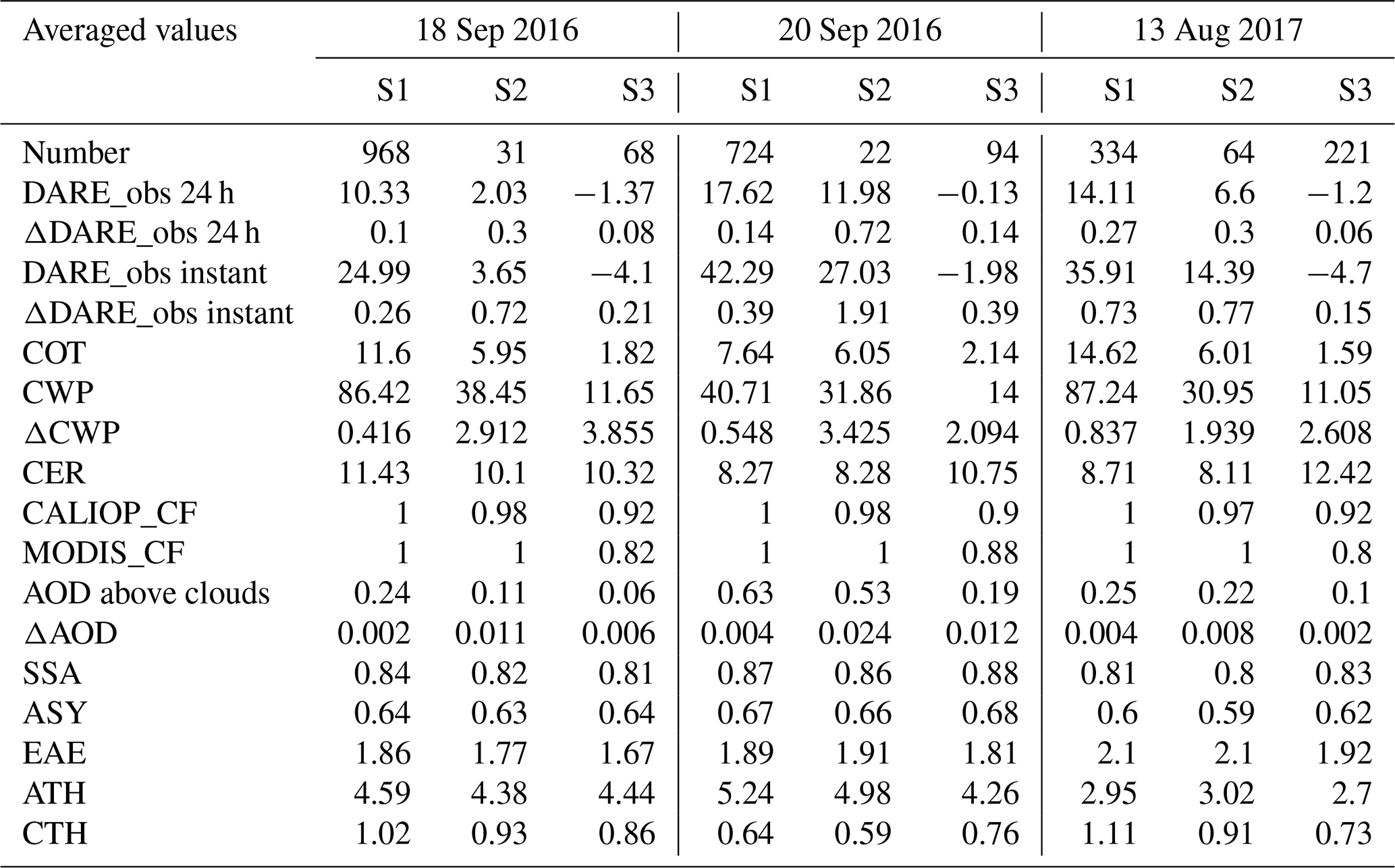
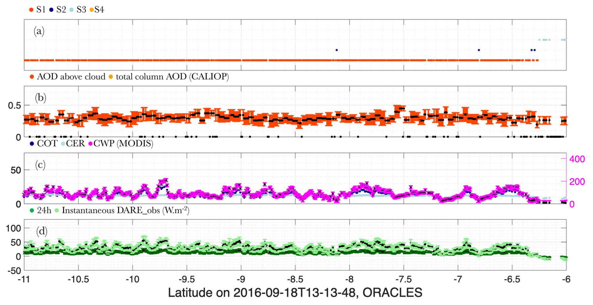
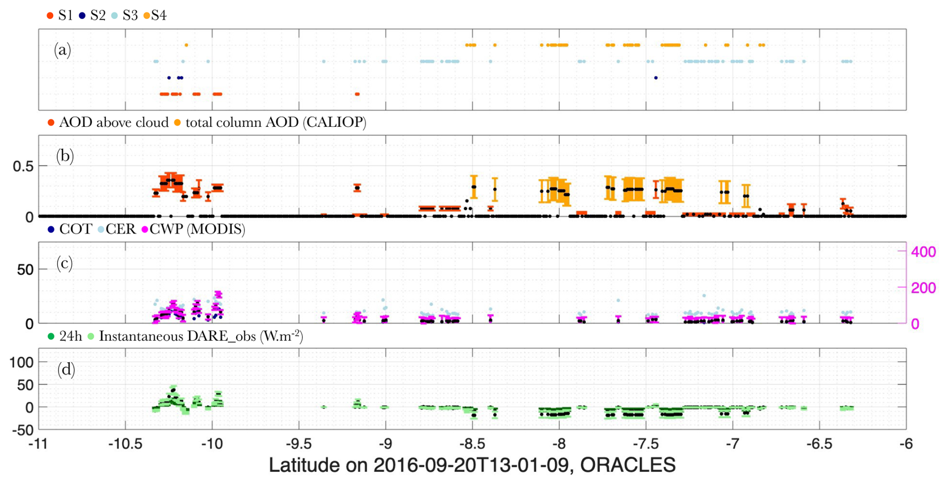
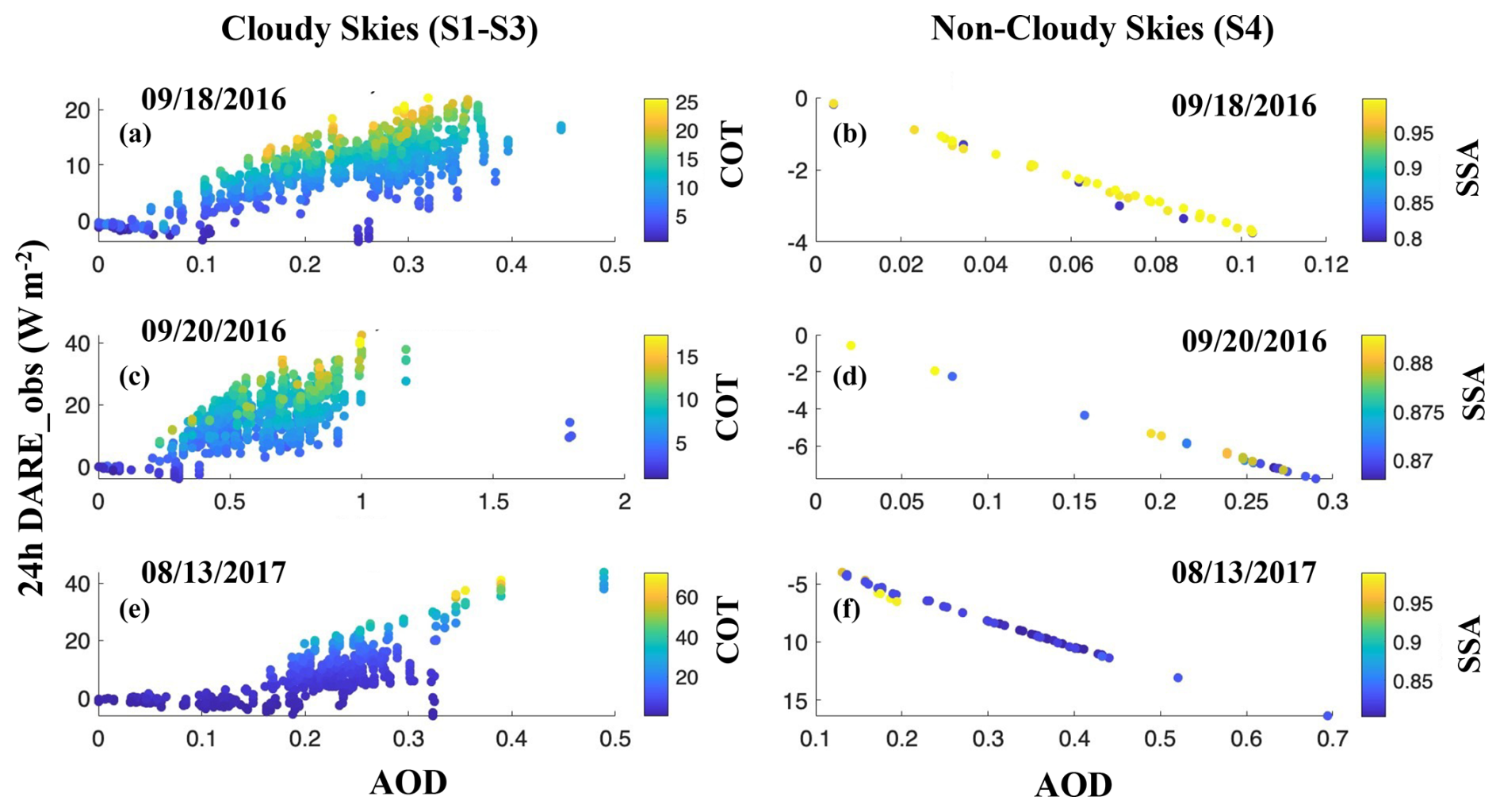
Figure A8 The 24 h DARE_obs in cloudy sky (S1–S3) (y axis) as a function of AOD (x axis) and COT (color bar) (a, c, e) and 24 h DARE_obs in non-cloudy sky (S4) (y axis) as a function of AOD (x axis) and SSA (color bar) (b, d, f) on 18 September 2016 (a, b), 20 September 2016 (c, d), and 13 August 2017 (e, f). Cloud-retrieved optical properties are not corrected for aerosols above them. Latitudes are selected between 6 and 20° S. AOD is at 532 nm; SSA and 24 h DARE_obs are in the 442–625 nm RRTMG channel; and SSA is selected at the highest aerosol height in MERRA-2.

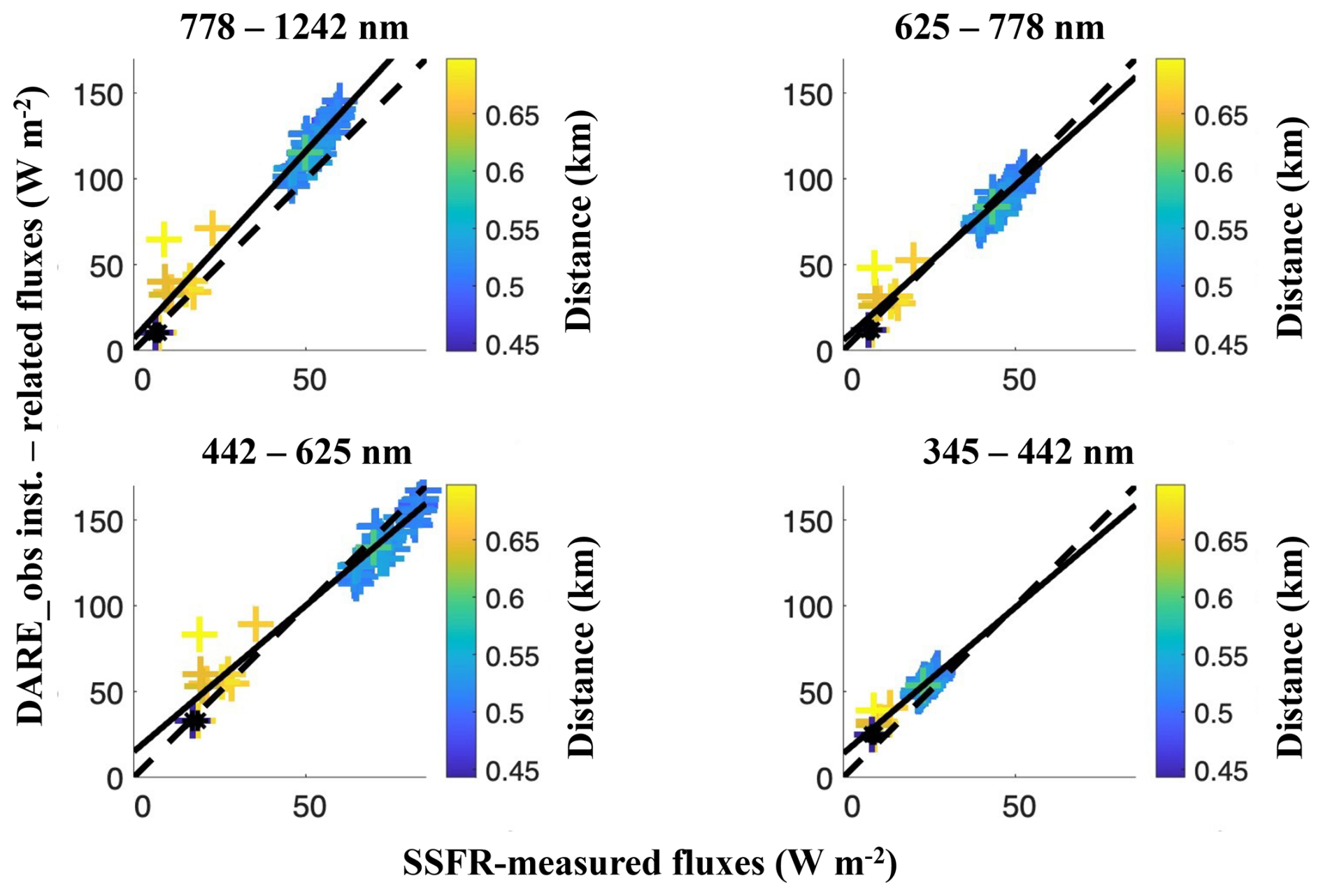
Figure A9 Instant SSFR-measured fluxes (x axis) vs. instant DARE_obs-related fluxes (W m⁻²) (y axis) in four RRTMG broadband channels (clockwise: 778–1242, 625–778, 345–442, and 442–625 nm). Points are colored by the distance between the aircraft and the CALIOP track (km). Black crosses are points in non-cloudy-sky conditions (S4). See second part of Table 6 in the text for statistics.