Local-scale inversion of agricultural ammonia emissions: a case study on Schiermonnikoog, the Netherlands

Quantifying real-world emission reductions is a core goal of atmospheric inversion methods, yet direct validation against known events remains rare, especially for reactive species like ammonia. In this study, we have applied local-scale Bayesian inversions using ground-based measurements and the LOTOS-EUROS air quality model, with high-resolution emission inventories as prior input, not to explore a theoretical scenario, but to evaluate a documented emission reduction. On the island of Schiermonnikoog in the Netherlands, where GVE (grazing livestock units) decreased from 639 to 541, with a particularly notable reduction in dairy cattle, ammonia emissions are expected a 23 % reduction between 2019 and 2022. Our inversion captured a similar trend, estimating a 51 % decrease, which may be overestimated, largely attributed to uncertainties in the 2019 posterior emissions. The posterior for 2022 shows consistency with the validation and indicates a 27 % reduction compared with the prior emissions of 2019. The associated uncertainty, derived from the posterior error covariance, highlights both the potential of the method and its limitations for policy verification. Moreover, we developed a method to assess the usefulness of individual observations and propose that adding a single high-quality continuous measurement in a strategically chosen location can significantly enhance the inversion performance. This strengthens the observational constraint and enhances the system’s ability to resolve temporal variations in emissions.

1 Introduction

Ammonia (NH₃) is a crucial component of the global nitrogen cycle, playing a fundamental role in agriculture and atmospheric chemistry. As the most abundant alkaline gas in the atmosphere, it significantly influences air quality, ecosystem health, and climate. Since discovery of the the synthesis of ammonia from atmospheric dinitrogen in 1908 (Haber, 1920), the application in fertilisers has revolutionised global food production, sustaining over half of the world's population (Erisman et al., 2008; Smil, 2004, 2002). However, this agricultural success comes at an environmental cost. The widespread use of synthetic fertilisers and intensification of livestock farming has led to increasing atmospheric ammonia emissions, with profound consequences for air pollution, nitrogen deposition, and climate change (Erisman et al., 2008, 2013; Zhang et al., 2020; McCubbin et al., 2002).

Understanding ammonia's behavior in the atmosphere remains challenging due to its high spatial and temporal variability. Once emitted, ammonia has a relatively short atmospheric lifetime; the average lifetime in the atmosphere is between a few hours and a few days (Dammers, 2017; Dammers et al., 2019; Zhang et al., 2021; Norman and Leck, 2005), and it can be rapidly deposited or converted into secondary particulate matter (Behera et al., 2013; Wyer et al., 2022). Its emissions are strongly influenced by meteorological conditions; for example, emission potential can increase by up to a factor of nine with a twenty-degree Celsius rise in temperature (Sutton et al., 2013; Ge et al., 2023). This leads to steep spatial gradients near sources, with concentrations varying significantly over distances of just a few kilometers (Schulte et al., 2022).

Traditional ammonia emission inventories rely on bottom-up estimates, which aggregate data from agricultural activities, industrial processes, and other sources based on production statistics and emission factors (Eggleston et al., 2006; Kuenen et al., 2022). However, these inventories suffer from inherent limitations. They often lack high temporal resolution, vary significantly between regions, and fail to capture the real-time dynamics of ammonia fluxes. Ammonia emissions are particularly sensitive to meteorological conditions, such as temperature and humidity, which can drive short-term fluctuations that are not well-represented in bottom-up models (Sutton et al., 2013; Ge et al., 2023).

To overcome these challenges, top-down approaches that integrate observational data into atmospheric models have gained traction. These methods use measurements from satellites and ground-based networks to constrain and refine emission estimates, offering a more dynamic and data-driven perspective on ammonia fluxes. Several studies have successfully applied top-down techniques to improve ammonia emission estimates. To name a few, Paulot et al. (2014) used the adjoint GEOS-Chem model with ammonium wet deposition fluxes to infer emissions across the United States, Europe, and China. Similarly, Zhang et al. (2018) combined satellite TES (Tropospheric Emission Spectrometer) data with inverse modeling to enhance ammonia emission inventories over China. More recently, van der Graaf et al. (2022) demonstrated the value of assimilating CrIS (Cross-track Infrared Sounder) ammonia retrievals into the LOTOS-EUROS chemistry transport model, significantly improving the spatial and temporal representation of emissions. Additionally, Cao et al. (2022) implemented a 4D-Var inversion that accounted for bi-directional ammonia fluxes, leading to an accurate depiction of seasonal variability in ammonia exchange between the surface and the atmosphere.

Despite these successes, most top-down studies have focused on global or mesoscale, leaving the need to understand ammonia emissions at localized scales where emission sources, meteorology, and deposition processes interact in complex ways. Moreover, quantifying real-world emission reductions is a core goal of atmospheric inversion methods, yet direct validation against known events remains rare, especially for reactive species like ammonia.

A particularly relevant case study is related to the nitrogen crisis in the Netherlands, where high ammonia emissions from agricultural activities have led to excessive nitrogen deposition, biodiversity loss, and regulatory interventions (Erisman, 2019; Stokstad, 2019; Erisman et al., 2021). Within this context, Schiermonnikoog, a small island in the north of the Netherlands, serves as an ideal testbed for ammonia emission reduction at a fine spatial scale, shown in Fig. 1. The largest part of the island falls under the National Park Schiermonnikoog, with rich landscapes that include dunes, beaches, forests, mudflats, and polders. The National Park is one of the most important nature areas in the Netherlands, and its habitats are sensitive to nitrogen deposition (Sival and Strijkstra-Kalk, 1999). However, intensive dairy farming in the island's 275 ha polder has historically contributed to ammonia loads exceeding critical thresholds (van Wijnen and Bakker, 1997).

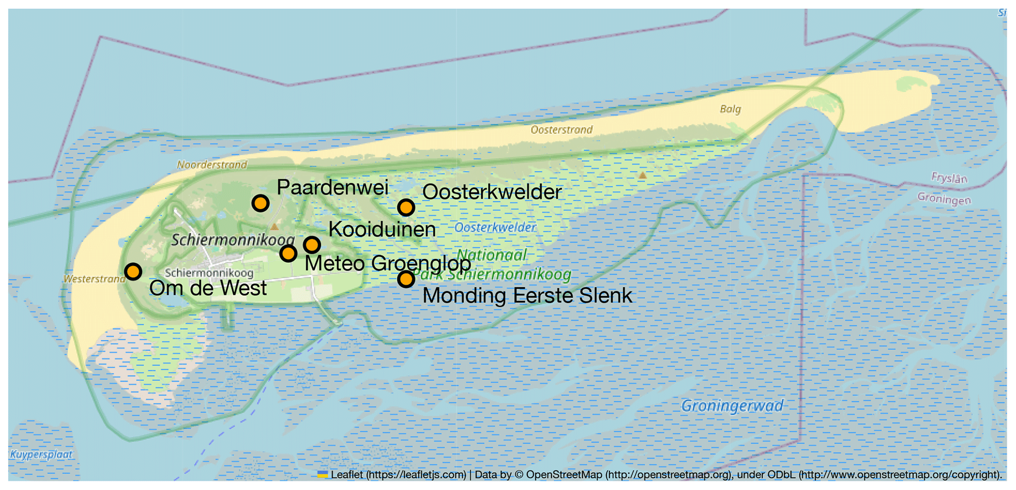
Figure 1 The map of Schiermonnikoog, in which the orange circles denote the MAN measurement sites, is provided by © OpenStreetMap contributors (2017). Distributed under the Open Data Commons Open Database License (ODbL) v1.0.

In response, a feasibility study by Erisman and Hofstee (2016) proposed nature-inclusive agricultural strategies to mitigate ammonia emissions while supporting the economic viability of local farmers. Although the transition began in 2016, a more pronounced reduction occurred between 2019 and 2022, during which GVE (grazing livestock units) decreased from 639 to 541, with dairy cattle numbers dropping from 510 to 363, according to KringloopWijzer data (van Dijk et al., 2023). These changes contributed to an estimated 23 % reduction in ammonia emissions, providing a valuable opportunity to evaluate whether current monitoring systems can effectively capture such changes and where improvements may be needed.

Despite the availability of satellite observations, retrieving reliable ammonia concentrations over small islands like Schiermonnikoog remains inherently challenging. The entire island and parts of the surrounding sea are captured within a single satellite footprint due to the limited land area of the island and the coarse spatial resolution of current satellite instruments. This spatial mismatch reduces the ability to resolve localized emission patterns. Moreover, the low ammonia column densities and weak thermal contrast between land and sea further degrade the retrieval quality and increase uncertainties in satellite-based NH₃ measurements (Van Damme et al., 2014). As for the ground-based measurements, no high-temporal resolution ammonia monitoring stations exist in the region, leaving monthly observations from the Measuring Ammonia in Nature (MAN) network as the only continuous source of in situ data (Lolkema et al., 2015; Noordijk et al., 2020). These ground-based measurements are crucial for validating and refining ammonia models at a local scale.

To bridge the gap between observations and models, we employ LOTOS-EUROS, a state-of-the-art regional chemistry transport model specifically designed for air quality applications in Europe. By combining MAN network data with LOTOS-EUROS simulations, we aim to refine spatial and temporal emission estimates, ultimately improving ammonia monitoring and mitigation strategies at the local scale.

In this study, we aim to refine local-scale ammonia emission estimates using a Bayesian inversion framework supported by atmospheric modeling and ground-based observations. We begin by simulating ammonia concentrations with LOTOS-EUROS and comparing them to measurements from the MAN network. To support the inversion, we generate controlled perturbation experiments to compute the Jacobian matrix and produce synthetic observations. These inputs allow us to quantify the model sensitivity and assess uncertainty through detailed error characterization. The inversion analysis proceeds in three stages:

• A comprehensive test incorporating MAN network uncertainties to evaluate model sensitivity.

• A refined inversion using real MAN network observations.

• A more optimized observation network design, outlining strategies to improve ammonia monitoring across different timescales.

These findings will provide valuable insights into the effectiveness of current monitoring networks and formulate future measurement strategies to better quantify ammonia emissions at fine temporal scales.

2 Data and Methodology

To evaluate ammonia emissions at a local scale, we use a Bayesian inversion framework combining atmospheric modeling, synthetic data experiments, and observational constraints. This chapter begins with an overview of real-world ammonia measurements from the MAN network, followed by a description of the synthetic data used for controlled tests. We then introduce the LOTOS-EUROS chemical transport model, along with the emission sources and prior estimates used in the simulations. Finally, we detail the inversion algorithm and the associated error characterisation.

2.1 Observations

2.1.1 In-situ measurements

The MAN (Measuring Ammonia in Nature) network is extensively used for monitoring atmospheric ammonia across the Netherlands. The spatial distribution of MAN sites is shown in Fig. 2. Unlike active optical techniques, the MAN network employs passive samplers, which measure monthly average ammonia concentrations via chemical absorption. This method is significantly cheaper than active optical techniques. Detailed descriptions of the measurement technique and associated uncertainties are provided in Lolkema et al. (2015) and Noordijk et al. (2020). In this study, we utilize monthly data from 26 MAN sites, 6 of which are located on Schiermonnikoog, for both annual and monthly emission inversion analyses.

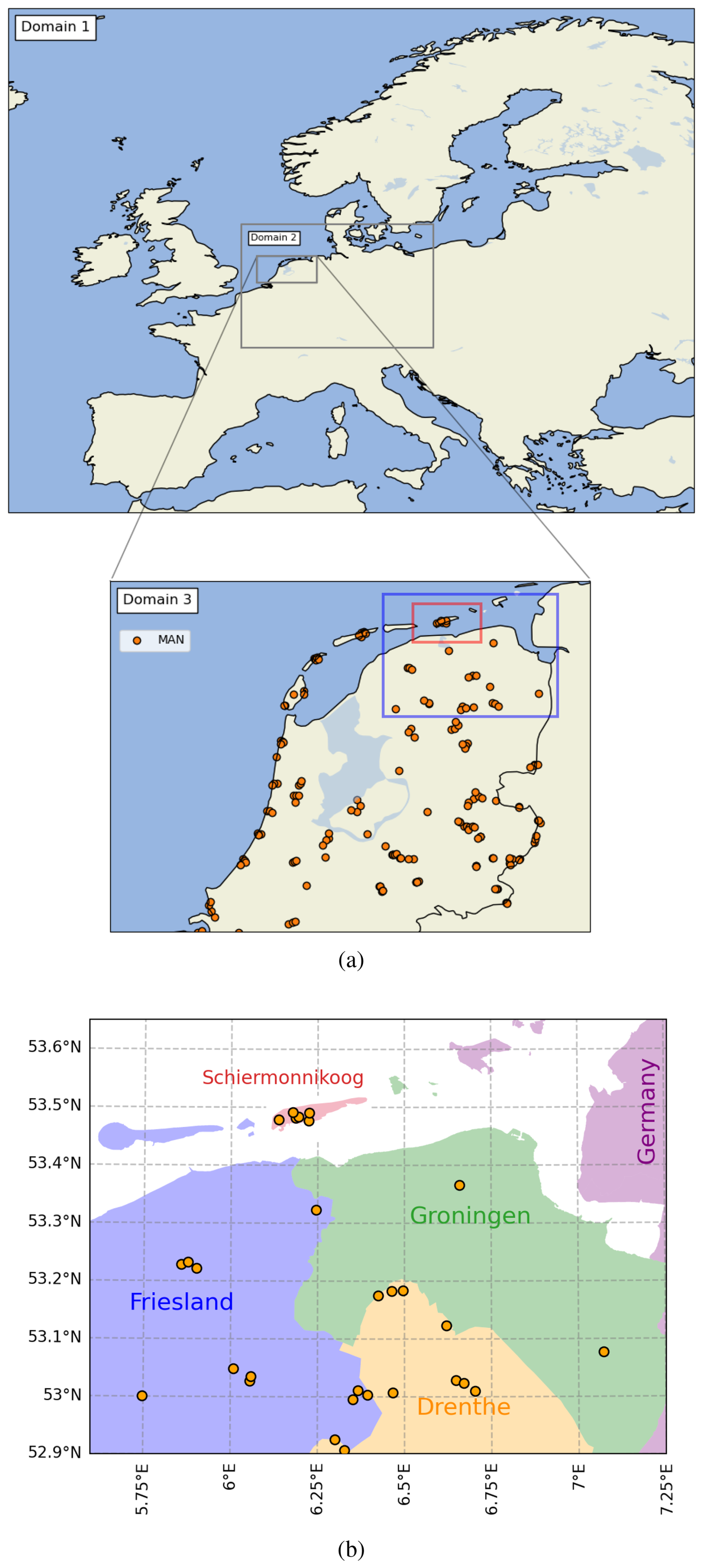
Figure 2 The nested domain configuration for LOTOS-EUROS simulation is shown in (a). In Domain 3, the orange circles denote the MAN measurement sites. Schiermonnikoog is located in the red box. The measurement located within the blue box are used for inversion, which is shown in (b) with Dutch provinces for source apportionment.

In addition to the MAN network, the Netherlands also employs optical measurement techniques with higher temporal resolution. The Dutch National Air Quality Monitoring Network (Landelijk Meetnet Luchtkwaliteit, LML) operates miniDOAS (active differential optical absorption spectroscopy) instruments, providing hourly ammonia concentrations (Berkhout et al., 2017; van Zanten et al., 2017). However, the LML network has far fewer monitoring sites compared to MAN. Since our study area lacks LML measurements, we introduce synthetic LML-like observations in the final section to explore their potential impact on inversion performance.

2.1.2 Simulated observations

To better understand the inversion process, we conducted a series of controlled tests using simulated observations. These tests were based on high-resolution hourly data, which were subsequently averaged into monthly values to align with the temporal scale of the MAN measurements. This setup enabled us to quantify observational uncertainties and assess how synthetic measurements can enhance the spatial and temporal coverage of the current monitoring network.

Using LOTOS-EUROS output, we generated synthetic “observational data” that mimic the current monitoring network. A configuration of the simulated errors is provided in:

$$\begin{array}{}\text{(1)}& s_{\text{full error}}=\sqrt{{\mathrm{0.90}}^{\mathrm{2}}+(\mathrm{0.28}\times c{)}^{\mathrm{2}}}\times \mathcal{N}(\mathrm{0},{\mathit{\sigma }}^{\mathrm{2}}),\end{array}$$

in which c is the surface concentrations, designed to reflect the existing MAN measurement error structure (Lolkema et al., 2015; Noordijk et al., 2020).

Additionally, we integrated LOTOS-EUROS output into the current monitoring framework as additional measurements, exploring its potential to support monitoring network design by providing high-resolution, high-quality measurement proxies.

2.2 LOTOS-EUROS

We use the state-of-the-art air quality model LOTOS-EUROS (LOng-Term Ozone Simulation and European Operational Smog model), developed by TNO, as the forward model in our inversion framework. This model integrates atmospheric transport, deposition, and chemical transformations of ammonia, providing a high-resolution framework for emission quantification. This study employs LOTOS-EUROS version 2.3.000, with its detailed configuration summarized in Table 1 (Manders et al., 2017; Manders-Groot and LOTOS-EUROS team, 2023).

The model is driven by Integrated Forecast System (IFS) from the European Centre for Medium-Range Weather Forecasts (ECMWF Hersbach et al., 2020). Three-hourly meteorological parameters are interpolated to one-hour resolution for finer temporal representation. To optimize computational efficiency and data storage, nested domains are used (Fig. 2): the coarsest domain covers from (35° N, 15° W) to (70° N, 35° E) with 0.5 and 0.25° resolution; the finest domain covers from (50.6° N, 3.15° E) to (53.7° N, 7.5° E) with 1.7 km × 2.15 km resolution.

Beyond standard air pollution modeling, one of key advantages is its source apportionment functionality, which allows for precise source attribution, distinguishing between agricultural, industrial, and natural contributions to ammonia concentrations. In this study, we use this function to track ammonia contributions from key regions:

• Countries: Germany, Denmark.

• Dutch regions: Schiermonnikoog, Groningen, Friesland, Drenthe, Gelderland, Overijssel (5 nearest provinces), and other locations.

Each emission source is further classified into two sectors: agricultural and non-agricultural emissions. This labeling framework enables precise source attribution and allows us to quantify the relative impact of various regions and sectors on ammonia concentrations over Schiermonnikoog. Detailed results are presented in Sect. 3.1.2.

Kuenen et al. (2022)Hersbach et al. (2020)

Table 1 LOTOS-EUROS model configuration

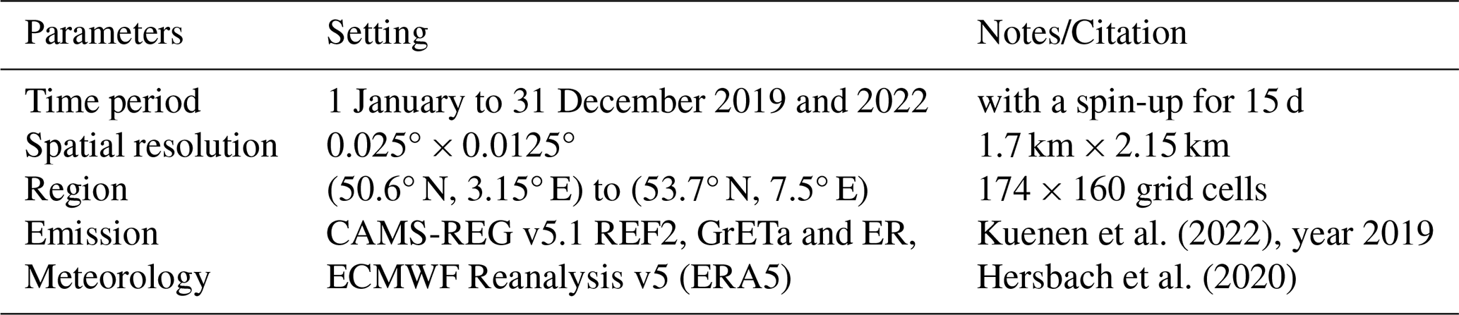
For spatial resolution, the first and second column denote (Δlon × Δlat) and (Δx × Δy), respectively.

2.3 Prior emission

The prior emissions used in the inversion, as well as the input for LOTOS-EUROS, are taken from the Copernicus Atmosphere Monitoring Service regional inventory (CAMS-REG v5.1 REF2, year 2019) for Domain 1 and GrETa and ER emission inventories for Domain 2 and 3. The temporal allocation follows the TNO-MACC (Monitoring Atmospheric Composition and Climate) inventory. This dataset includes emissions of major air pollutants, with detailed information available in Kuenen et al. (2021, 2022). The emissions are provided with a spatial resolution of 0.0167° × 0.0083° in the finest domain.

In this study, we only optimize ammonia emissions from agricultural sources, as they are the dominant contributor to atmospheric NH₃. Other emission sectors – traffic, residential, industrial, and transportation – are categorized as non-agricultural emissions Further details on the agricultural sector are provided in the Supplement; more details can be refered to Kuenen et al. (2022, 2021).

2.4 Bayesian Inversion algorithm

To optimize annual and monthly ammonia emissions using observational constraints, we apply a Bayesian inversion framework, which efficiently integrates errors from prior emissions, observations, and the model itself. This approach is highly flexible, allowing for its application at local scales with different observational datasets.

Bayesian inversion aims to estimate the posterior probability density function (pdf) of the state vector x given observations y. The revised version is expressed as (Rodgers, 2000; Turner and Jacob, 2015):

$$\begin{array}{}\text{(2)}& \begin{array}{rl}P\left(\mathit{x}\right|\mathit{y})& ={\displaystyle \frac{P\left(\mathit{y}\right|\mathit{x}\left)P\right(\mathit{x})}{P\left(\mathit{y}\right)}}\\ & \propto \exp \mathit{\{}-(\mathit{x}-{\mathit{x}}_{\mathrm{a}}{)}^T{{\mathbf{S}}_{\mathrm{a}}}^{-\mathrm{1}}(\mathit{x}-{\mathit{x}}_{\mathrm{a}})\\ & -[\mathit{y}-\mathbf{F}(\stackrel{\circ }{\mathit{x}}\left){]}^T{{\mathbf{S}}_{\mathrm{O}}}^{-\mathrm{1}}\right[\mathit{y}-\mathbf{F}\left(\stackrel{\circ }{\mathit{x}}\right)\left]\mathit{\right\}},\end{array}\end{array}$$

where:

• $\stackrel{\circ }{\mathit{x}}$, the actual (linear) state vector, is defined as the scaling factor that represents the ratio of posterior to prior of each label. Additional state vector elements are defined in Sect. “Error covariance matrices”;

• x is defined in logarithmic space such that $\mathit{x}=\ln \left(\stackrel{\circ }{\mathit{x}}\right)$. This log transformation ensures positivity and accommodates multiplicative uncertainty in emissions;

• y is the vector with observations, which is monthly data from 26 MAN sites;

• F operates on $\stackrel{\circ }{\mathit{x}}$, to simulate corresponding concentrations;

• x_a is the prior state vector in logarithmic form;

• S_a and S_O are the prior and observational error covariance matrices, respectively (details in Sect. “Error covariance matrices”).

The optimal state x is found by maximizing Eq. (2), which corresponds to minimizing the cost function:

$$\begin{array}{}\text{(3)}& \begin{array}{rl}\mathcal{J}\left(\mathit{x}\right)& =(\mathit{x}-{\mathit{x}}_{\mathrm{a}}{)}^T{\mathbf{S}}_{\mathrm{a}}^{-\mathrm{1}}(\mathit{x}-{\mathit{x}}_{\mathrm{a}})\\ & +[\mathit{y}-\mathbf{F}(\stackrel{\circ }{\mathit{x}}\left){]}^T{\mathbf{S}}_{\mathrm{O}}^{-\mathrm{1}}\right[\mathit{y}-\mathbf{F}\left(\stackrel{\circ }{\mathit{x}}\right)],\end{array}\end{array}$$

where x is of shape (n×1); y is (m×1); S_a is (n×n); S_O is (m×m). We then approximate $\mathbf{F}\left(\stackrel{\circ }{\mathit{x}}\right)$ linearly with a Jacobian matrix $\stackrel{\circ }{\mathbf{K}}$ (m×n), thus:

$$\begin{array}{}\text{(4)}& \mathbf{K}={\mathrm{\nabla }}_{\mathit{x}}\mathbf{F}={\displaystyle \frac{\partial \mathit{y}}{\partial \mathit{x}}}={\displaystyle \frac{\partial \mathit{y}}{\partial \left(\ln \stackrel{\circ }{\mathit{x}}\right)}}=\stackrel{\circ }{\mathbf{K}}\mathrm{diag}\left(\stackrel{\circ }{\mathit{x}}\right),\end{array}$$

where K is the Jacobian matrix in logarithmic space; $\stackrel{\circ }{\mathbf{K}}$ is the Jacobian in linear space, defined as ${\stackrel{\circ }{K}}_{ij}=\partial {\mathit{y}}_{\left(i\right)}/\partial {\stackrel{\circ }{\mathit{x}}}_{\left(j\right)}$, which is constructed with an one-sided perturbation of 40 %. Notably, for monthly emission inversions, the Jacobian is defined as a block diagonal matrix so that each month is considered independent.

To solve the Eq. (3), we apply the Levenberg–Marquardt approach (Rodgers, 2000; Chen et al., 2022, 2023), iteratively updating the state vector:

$$\begin{array}{}\text{(5)}& \begin{array}{rl}{\mathit{x}}_{N+\mathrm{1}}& ={\mathit{x}}_N+[{\mathbf{K}}_N^T{\mathbf{S}}_{\mathrm{O}}^{-\mathrm{1}}{\mathbf{K}}_N+(\mathrm{1}+\mathit{\kappa }){\mathbf{S}}_{\mathrm{a}}^{-\mathrm{1}}{]}^{-\mathrm{1}}\\ & \cdot \left[{\mathbf{K}}_N^T{\mathbf{S}}_{\mathrm{O}}^{-\mathrm{1}}\right(\mathit{y}-\stackrel{\circ }{\mathbf{K}}\stackrel{\circ }{\mathit{x}})-{\mathbf{S}}_{\mathrm{a}}^{-\mathrm{1}}({\mathit{x}}_N-{\mathit{x}}_{\mathrm{a}}\left)\right],\end{array}\end{array}$$

where x_N is the state vector at the Nth iteration; K_N is the Jacobian matrix at the Nth iteration, which updates accordingly through ${\mathbf{K}}_N=\stackrel{\circ }{\mathbf{K}}\mathrm{diag}\left({\stackrel{\circ }{\mathit{x}}}_N\right)$, following Eq. (4); κ is the coefficient for determining the convergence rate and is set as 10 (Chen et al., 2022); $\stackrel{\circ }{\mathbf{K}}\stackrel{\circ }{\mathit{x}}$ is equivalent to the forward model. The uncertainty in the optimized emissions is given by the posterior error covariance matrix:

$$\begin{array}{}\text{(6)}& \widehat{\mathbf{S}}=({\mathbf{K}}_N^T{\mathbf{S}}_{\mathrm{O}}^{-\mathrm{1}}{\mathbf{K}}_N+{\mathbf{S}}_{\mathrm{a}}^{-\mathrm{1}}{)}^{-\mathrm{1}},\end{array}$$

where K_N is the Jacobian at the final iteration. The degree of freedom for signal (DFS) is then calculated from:

$$\begin{array}{}\text{(7)}& \mathrm{DFS}=\mathrm{trace}\left(\mathbf{A}\right),\end{array}$$

where A is the averaging kernel matrix:

$$\begin{array}{}\text{(8)}& \mathbf{A}={\displaystyle \frac{\partial \widehat{\mathit{x}}}{\partial \mathit{x}}}=\mathbf{I}-\widehat{\mathbf{S}}{\mathbf{S}}_{\mathrm{a}}^{-\mathrm{1}}.\end{array}$$

The DFS quantifies how much information is gained from the observations. Higher DFS values indicate a stronger observational constraint on the emissions.

Error covariance matrices

The state vector in our inversion framework includes not only agricultural emissions from Schiermonnikoog but also contributions from external sources. These external influences are determined using the labeling functionality in the LOTOS-EUROS model, which identify regions that significantly impact ammonia concentrations on the island. If a labeled area has a strong contribution to Schiermonnikoog's ammonia levels, then uncertainties in emissions from that region are likely to propagate to the island's atmospheric NH₃ concentrations. Here, we define the criteria: $c_{\mathrm{label}}/c_{\mathrm{total}}>\mathrm{10}$ %. For labeled concentrations larger than 10 % of the total concentration, the labels are selected as the external influences, of which the result can be found in Sect. 3.1.2. Thus, the state vector is constructed with five elements, where the first represents the local emission source and the remaining four represent external influences to fix the boundary condition:

1. agricultural emissions from Schiermonnikoog;

2. total contribution to concentration (agricultural and non-agricultural) from Groningen;

3. total contribution to concentration from Friesland;

4. total contribution to concentration from Germany;

5. a composite term (“Other”) representing contributions to concentration from all remaining sources and sectors.

A major source of uncertainty in ammonia emissions are volatilization rates, which varies with temperature. The re-emission potential can increase by a factor of 9 for a twenty degrees Celsius temperature rise (Ge et al., 2023; Sutton et al., 2013). To account for this variability, and given the use of a logarithmic state vector, the prior error covariance matrix S_a is constructed to a diagonal matrix with terms defined as (ln β)², where β=2 represents the assumed annual emission variability factor, while external influences are assigned a factor of 1.5. For monthly emission inversion, the variability factors are set to β=4 for emissions and 2 for external influences.

To estimate the observational error covariance matrix S_O, we first follow the commonly used residual error method (Brasseur and Jacob, 2017):

$$\begin{array}{}\text{(9)}& {\mathbf{S}}_{\mathrm{O}}=E\left[\mathit{\epsilon }{\mathit{\epsilon }}^T\right],\end{array}$$

where:

• $\mathit{\epsilon }=(\mathit{z}-\stackrel{\mathrm{‾}}{\mathit{z}})$ is the residual error vector, assumed to represent random noise;

• $\mathit{z}=\mathit{y}-\mathbf{F}\left(\stackrel{\circ }{\mathit{x}}\right)$ denotes the misfit between observations and forward model output, assuming discrepancies arise primarily from emission uncertainties.

Initially, S_O is constructed using only diagonal elements with the residual error vector. However, this simplification introduces potential uncertainties. To improve representativeness, we adopt a hybrid approach that combines (1) residual error estimates and (2) established uncertainty descriptions from the MAN network (Noordijk et al., 2020; Lolkema et al., 2015). This integrated error representation enhances the robustness of the inversion system but might also overestimate the total uncertainty.

To assess the performance of this combined error formulation, we perform a series of χ² tests and optimize the integrated observational error to ensure an appropriate balance between model constraints and observational uncertainties (Rodgers, 2000). The total observational error is formulated as:

$$\begin{array}{}\text{(10)}& \mathit{\epsilon }=\sqrt{{\mathit{\epsilon }}_{\mathrm{residual}}^{\mathrm{2}}+(\mathit{\alpha }\cdot {\mathit{\epsilon }}_{\mathrm{MAN}}{)}^{\mathrm{2}}},\end{array}$$

where:

• ${\mathit{\epsilon }}_{\mathrm{residual}}=(\mathit{z}-\stackrel{\mathrm{‾}}{\mathit{z}})$;

• ${\mathit{\epsilon }}_{\mathrm{MAN}}=\sqrt{{\mathrm{0.90}}^{\mathrm{2}}+(\mathrm{0.28}\times \mathit{c}{)}^{\mathrm{2}}}$, with c the monthly ammonia concentrations;

• α is a scaling factor optimized to best match model and observational uncertainty.

We define a performance score $s_{{\mathit{\chi }}^{\mathrm{2}}}$ to simultaneously evaluate statistical consistency (via p-value) and goodness-of-fit (via normalized χ², NCS):

$$\begin{array}{}\text{(11)}& s_{{\mathit{\chi }}^{\mathrm{2}}}=p\cdot e^{-|\mathrm{1}-\mathrm{NCS}|},\end{array}$$

where:

• p is the p-value from χ² tests;

• $\mathrm{NCS}=\frac{{\mathit{z}}^T{\mathbf{S}}_{\mathrm{O}}^{-\mathrm{1}}\mathit{z}}{\mathrm{DOF}}$, with DOF as degrees of freedom.

This score reaches a maximum when both the model-observation agreement is close to ideal (NCS≈1) and the residuals are consistent with the assumed error distribution (high p-value). Note that here, DOF refers to the number of independent observational constraints used in the χ² calculation, and should not be confused with DFS, degrees of freedom for signal defined in Eq. (7), which measures how much information from observations is retained in the state vector after inversion. While both reflect aspects of information content, they apply to different parts of the inversion framework.

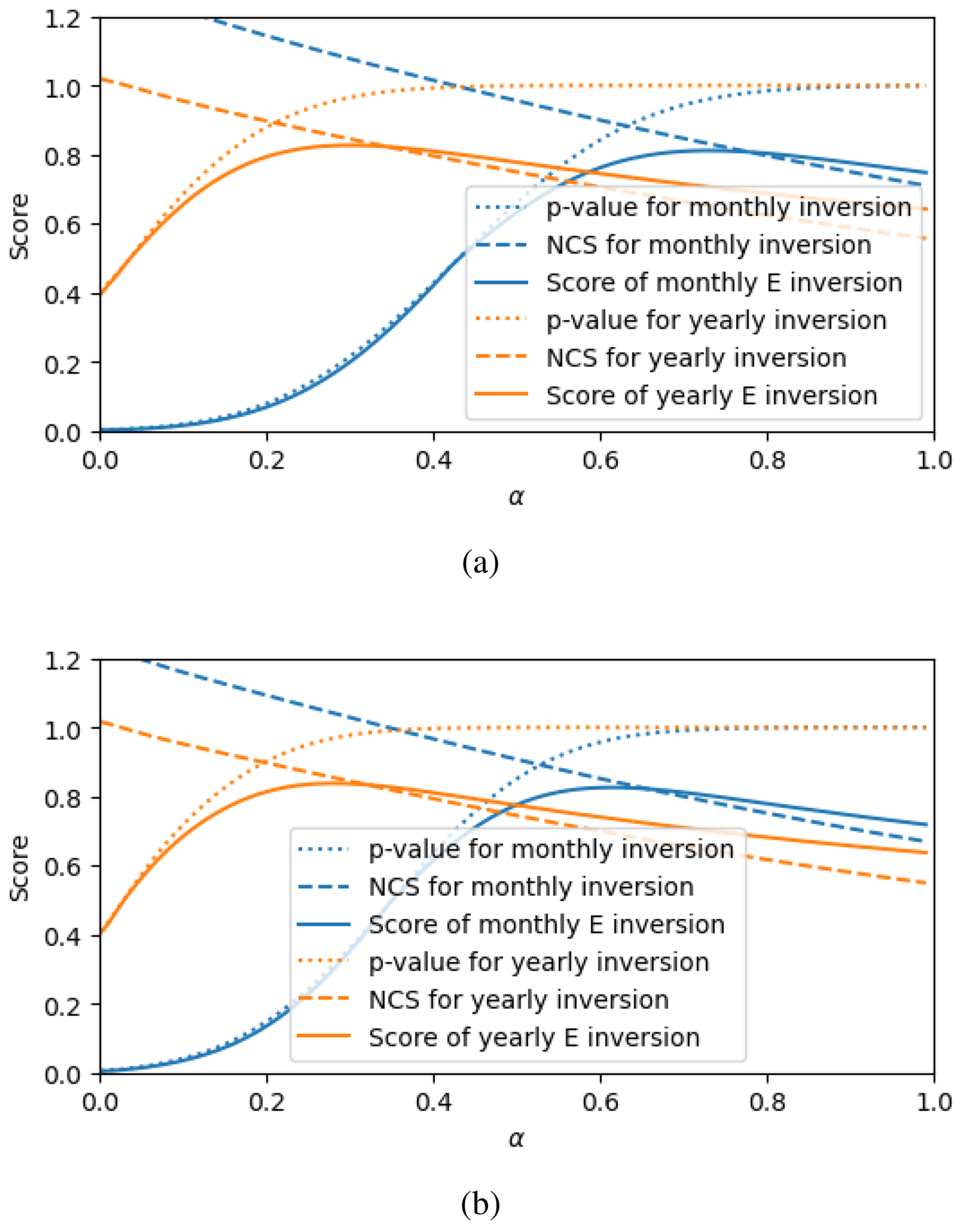
Figure 3 Evaluation of χ² test results in 2019 (a) and 2022 (b) for the total observational error defined in Eq. (10). The model performance is scored by Eq. (11). A score is derived from the p-value and the normalized χ² (NCS). An NCS value near 1 and a p-value close to 1 indicate that the error description is reasonable, reflecting a good fit and appropriate error covariance. Notably, the August and July 2019 data are eliminated because of the dune fire in 2019.

Based on the optimization (Fig. 3), we assign: for monthly emission inversions α=0.5; for annual emission inversions, α=0.3), reflecting the averaging over longer periods and the reduced influence of short-term fluctuations. For simulated observations, α=0.3 for monthly inversions and α=0.15 for annual inversions, reflecting the lower uncertainty in synthetic data compared to real-world observations. These adjustments ensure that the inversion framework maintains robustness while adequately capturing observational uncertainties across different timescales. Similar to Fig. 3, the optimization of χ² statistics of simulated observations can be found in the Supplement.

3 Results and Discussions

In this section, we first present the simulated results of the LOTOS-EUROS model, including the source apportionment output. Next, we validate the inversion framework using synthetic errors and simulated data. We then apply MAN measurements to perform the inversion on real-life data, analyze emission reductions, and investigate emission estimates across different timescales. Finally, we explore potential improvements to the inversion framework and propose an optimized observational design for enhanced emission monitoring.

Table 2 The statistics of comparison between the simulation of prior emissions with LOTOS-EUROS and the MAN measurements with the prior emission, including Pearson's correlation coefficient (r), root-mean-square error (RMSE), mean absolute error (MAE), mean absolute percentage Error (MAPE), normalized mean bias (NMB) and slope.

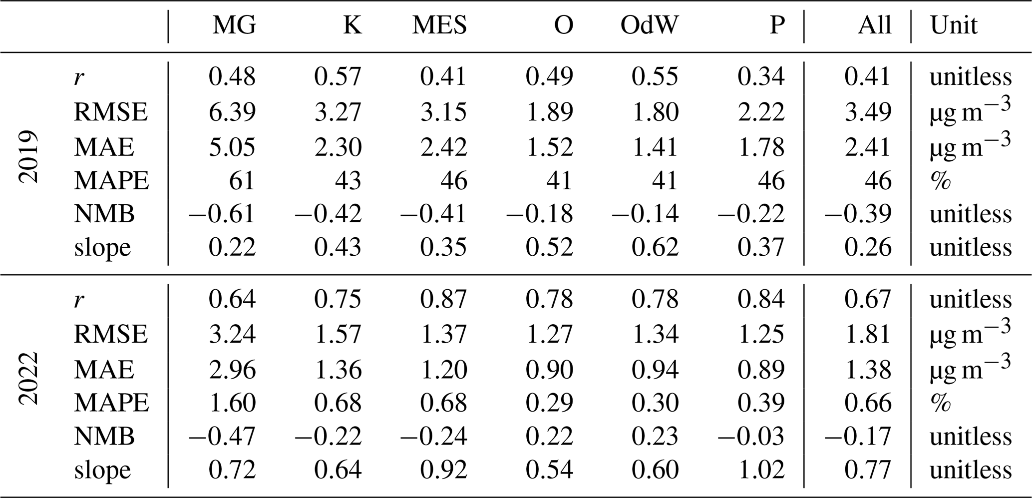
The abbrevations correspond to the site names: Schiermonnikoog-Meteo Groenglop, -Kooiduinen, -Monding Eerste Slenk, -Oosterkwelder, -Om de West, -Paardenwei.

3.1 Model performance and source apportionment with the prior emission

To evaluate the representativeness of the meteorological forcing, model results were compared with observations from nearby KNMI stations on a daily basis (map shown in Fig. S1 in the Supplement), including one located close to the island. The agreement was very good, with correlations for wind components, temperature, and pressure consistently above 0.96 and low RMSE values (Table S2, Fig. S2 in the Supplement). Precipitation was also well reproduced, with correlations around 0.8. These results indicate that the meteorological fields are reliable and representative for the study area, supporting the robustness of the subsequent analysis.

3.1.1 Model performance

Figure S3 illustrates the monthly variation of prior ammonia emissions and corresponding surface concentrations on Schiermonnikoog for 2019 and 2022. In both years, agricultural emissions peaked in March, following model time profile, with a secondary, smaller peak in August. Other local emissions, including non-agricultural sources, remain constant through the year. These emission patterns directly influence surface ammonia concentrations, which follow a characteristic bimodal seasonal cycle: a spring peak associated with manure spreading and a summer peak driven by higher temperatures and volatilization. Notably, although the same emission inventory is applied for both years, the emission rates vary greatly due to differences in the meteorological conditions under which the rates are calculated (Skjøth et al., 2011).

To evaluate the performance of the LOTOS-EUROS model in simulating ammonia concentrations, a statistical comparison was conducted against MAN network measurements. The assessment included Pearson's correlation coefficient (r), root-mean-square error (RMSE), mean absolute error (MAE), mean absolute percentage error (MAPE), normalized mean bias (NMB), and the slope of the regression between simulated and observed values. Table 2 presents the statistical results for six monitoring sites on Schiermonnikoog in both 2019 and 2022.

In 2019, the correlation coefficient (r) ranged from 0.34 to 0.55 across sites, reflecting a moderate agreement between model predictions and observations. By 2022, correlation values reached up to 0.87 at certain locations. Notable discrepancies occur, particularly at sites located near strong emission sources, such as Meteo Groenglo. This site consistently exhibited the highest RMSE and NMB values in both years, indicating that the spatial resolution of the model may not adequately capture local-scale variability in emissions. In 2019, the underestimation of peak ammonia concentrations is reflected in the strongly negative NMB values and correlation. This bias was reduced in 2022, especially at sites farther from major emission sources. Furthermore, the slope of the regression line between simulated and observed concentrations increased in 2022. The difference between two years may be due to an unaccounted-for occurrence of ammonia emission.

Digging deeper, a comparison of modeled and observed ammonia concentrations is illustrated in Fig. 4. The scatter plots for 2019 (a) and 2022 (c) demonstrate that the model underestimated ammonia concentrations in high-emission months, particularly during summer. The regression lines fitted in the scatter plots confirm that the model performed better in 2022, aligning more closely with the 1 : 1 reference line. Monthly variations, as shown in the right-hand panels of Fig. 4b and d, reveal that while the model captured the seasonal cycle of ammonia, it underestimated peak concentrations in summer and overestimated lower values in winter. These discrepancies suggest that an improvement in the temporal variations of the emissions is needed.

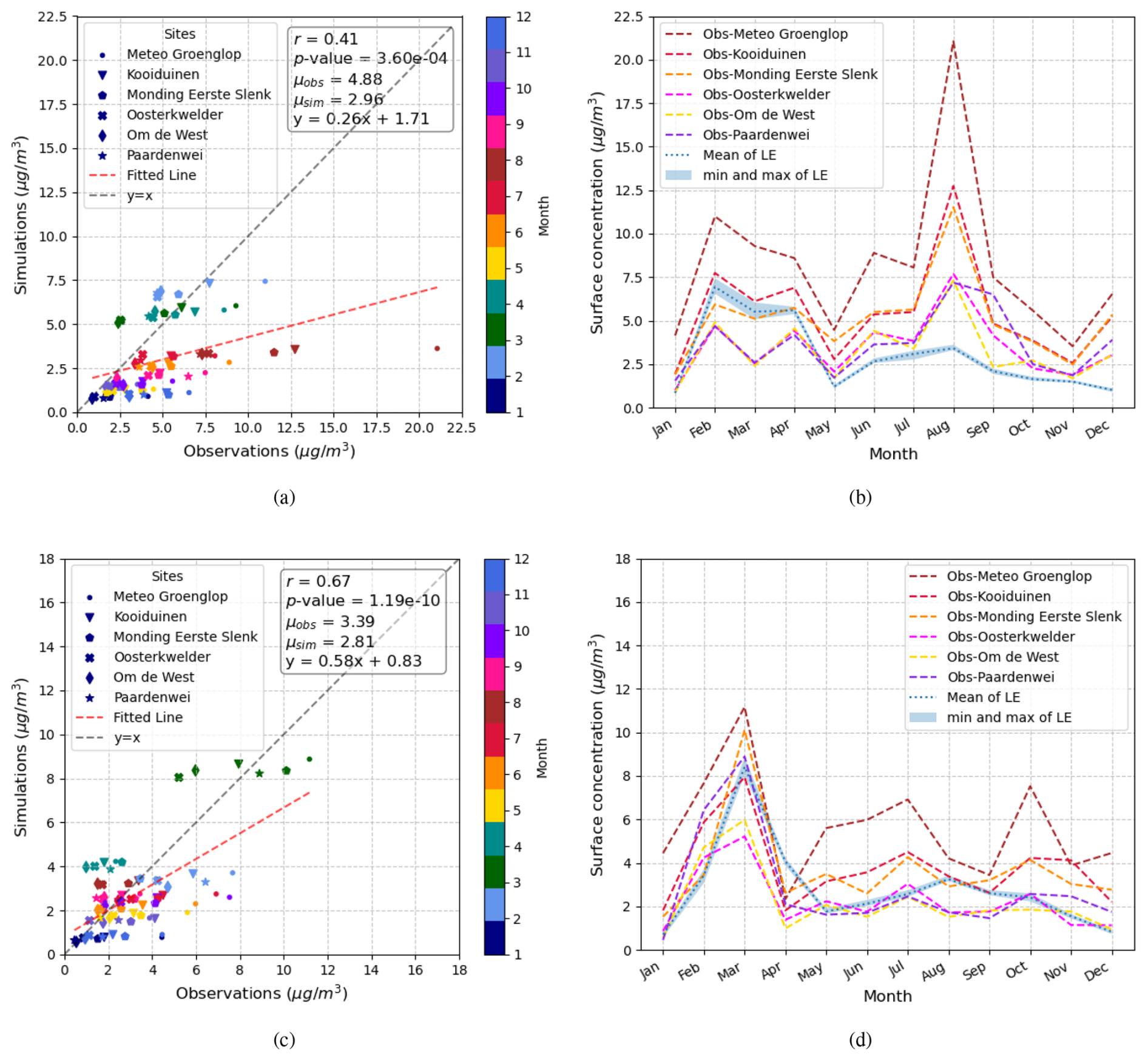
Figure 4 The comparison of model and observation in monthly average on Schiermonnikoog with the prior emission in 2019 (a, b) and 2022 (c, d).

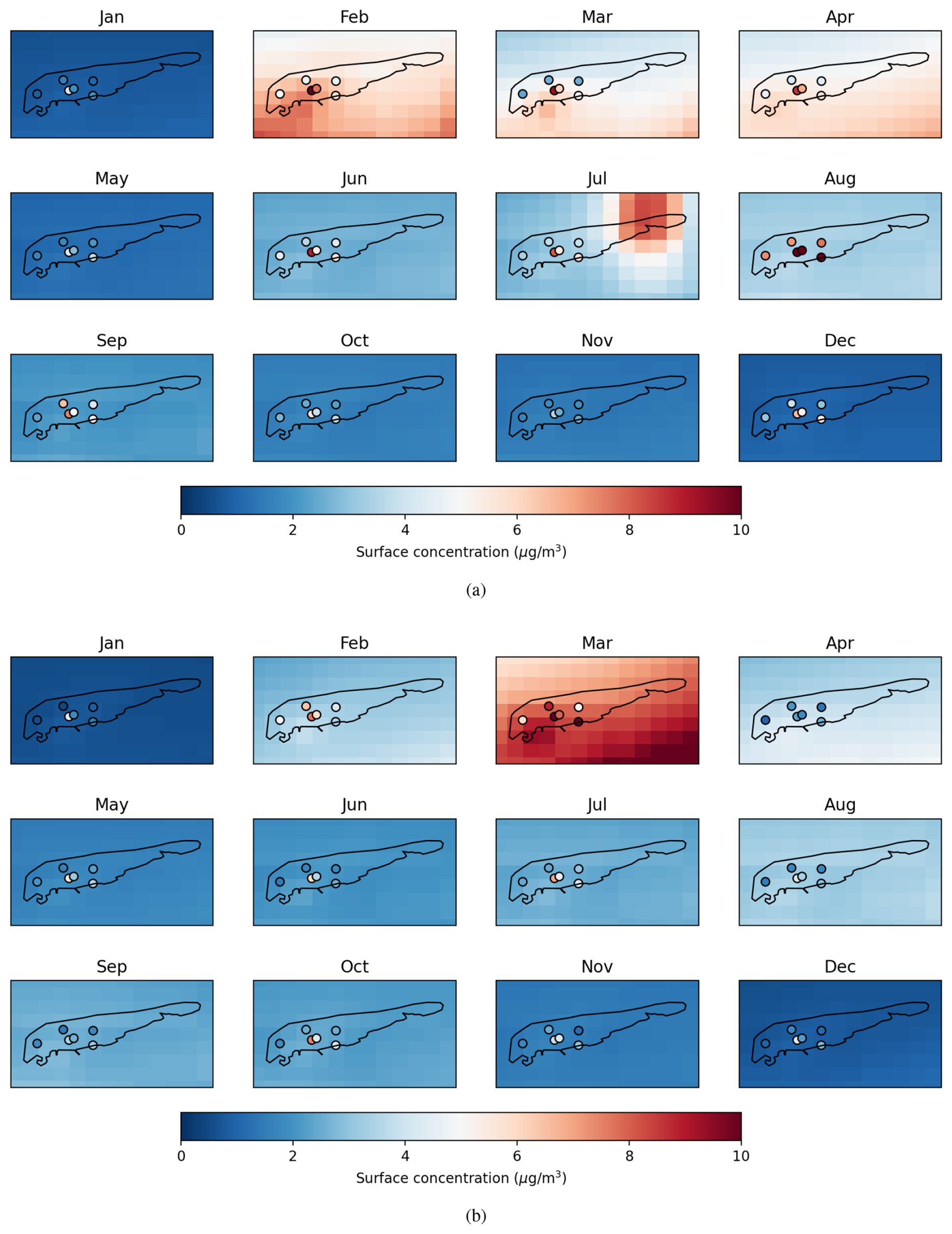
Figure 5 Maps of simulated surface concentrations on Schiermonnikoog for 2019 (a) and 2022 (b) with the prior emission.

In addition to statistical performance, spatial variability was examined as shown in Fig. 5. These maps illustrate the modeled ammonia concentrations across Schiermonnikoog for each month in 2019 and 2022, overlaid with MAN measurement locations. The maps highlight a clear seasonal pattern, with elevated concentrations during spring and summer, consistent with agricultural activity and temperature-driven volatilization. The spatial distribution of ammonia shows gradients, particularly in regions downwind of emission sources. The comparison between modeled fields and observations suggests that while LOTOS-EUROS effectively captures broad seasonal trends, local-scale concentration hotspots remain difficult to resolve due to the inadequate spatial resolution of the simulation, especially near emission sources. As shown in Fig. S4, the spatial resolution of the emission inventory does not always align with the true distribution of local ammonia sources, particularly on Schiermonnikoog, where emissions from agricultural activities are concentrated in a small area. Since the model operates on a coarser grid, emissions may be spread over a larger area or displaced from their actual sources, leading to an underestimation of concentration peaks at specific measurement sites. This is particularly evident at the Schiermonnikoog-Meteo Groenglop site, where observed ammonia levels are consistently higher than simulated values, likely due to its proximity to actual emission sources that are not well-represented in the model. To assess the potential impact of spatial resolution, we conducted additional simulations using a nested domain with 500 m × 500 m resolution over Schiermonnikoog (see the Supplement). The results indicate only limited improvement compared to the coarser-resolution setup: the Pearson correlation and regression slope with observations increased slightly, but overall scatter remained similar. This limited gain is mainly due to the coarser resolution of the emission inventory, which constrains the benefit of refining the model grid. Therefore, for consistency, we present the results from the coarser-resolution simulations (with bi-cubic interpolation) in the main analysis.

Moreover, external factors may have contributed to the high discrepancies observed in specific months. For instance, in July 2019 (see Fig. 5a), dune fires occurred in the eastern dunes of Schiermonnikoog, leading to increased ammonia concentration. Although fires were accounted for in the model with Global Fire Assimilation System (GFAS) emission inventory (Kaiser et al., 2012), the simulation remains highly uncertain due to the complexity of fire-induced emissions. Additionally, the timing of passive sampler collection in the MAN network may not always align strictly with the first and last days of the month, potentially introducing inconsistencies between measured and simulated values.

3.1.2 Source Apportionment of Ammonia Concentrations

To better understand the origins of ammonia concentrations on Schiermonnikoog, a detailed source apportionment analysis was conducted, using the LOTOS-EUROS model's labeling function. Figure 6 presents both the monthly variations in source contributions (panels a, b) and the annual summaries (panels c, d) for 2019 and 2022. These results reveal that local emissions play a relatively minor role in the island’s ammonia budget, with the majority of the observed concentrations originating from external sources.

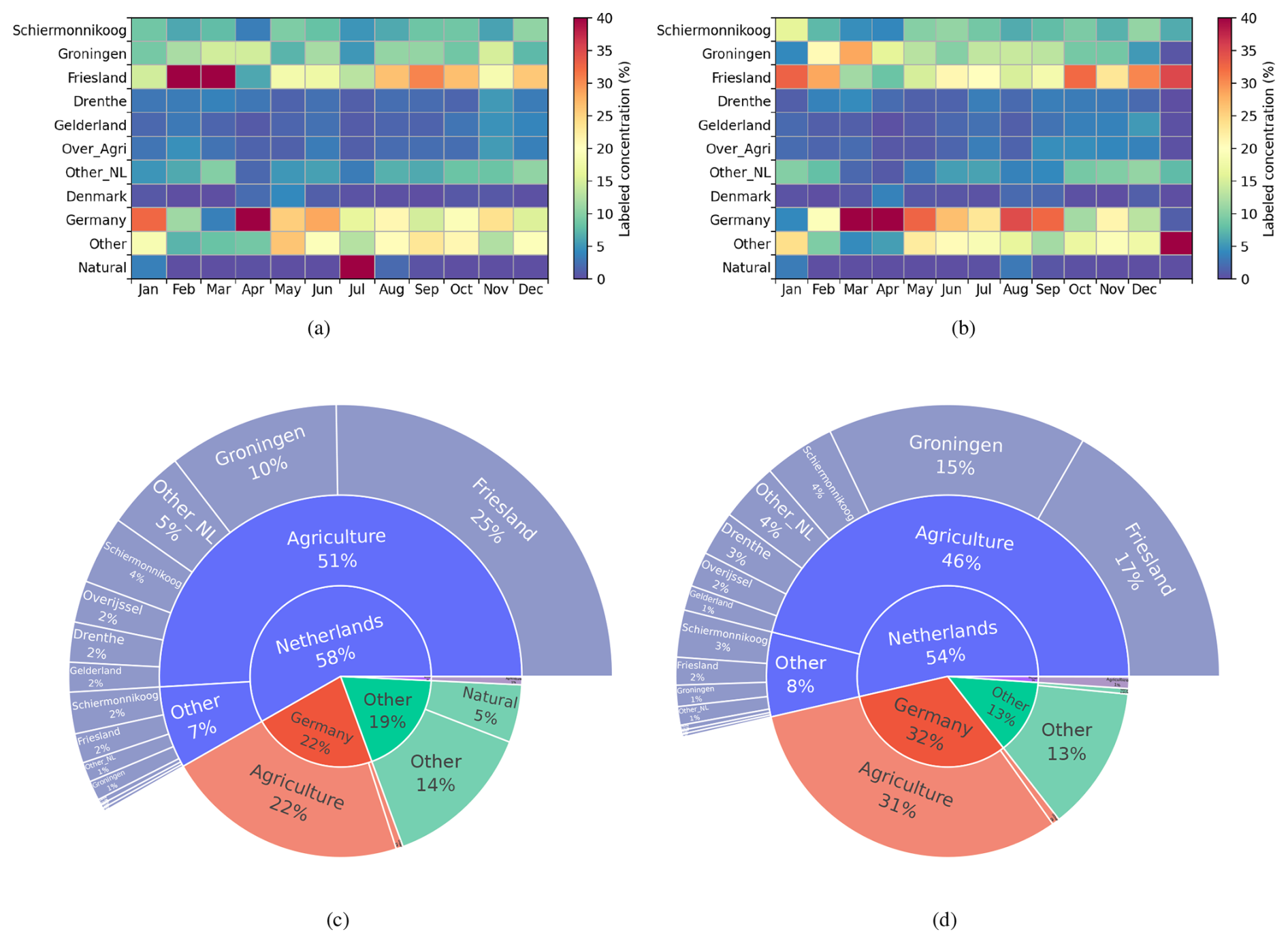
Figure 6 The relative contributions of different sources to the surface concentration of Schiermonnikoog in 2019 (a, c) and 2022 (b, d) simulated by LOTOS-EUROS with the prior emission. Each row in the monthly panels (a) and (b) shows the label's overall contribution, which includes emissions from the agricultural and other sectors. Panels (c) and (d) show the annual results.

In 2019, emissions from Schiermonnikoog itself accounted for 6 % of annual ammonia concentrations, with 4 % from agriculture and 2 % from other activities. Transported emissions from Friesland, Groningen, and Germany collectively contributed over 50 %, with Friesland consistently showing the highest contribution, followed by Germany and Groningen. The distribution was similar in 2022, though with a slight reduction in emissions from natural sources, primarily due to a lower frequency of wildfire events compared to 2019. A particularly significant contributor across both years was the “Other” label, representing over 10 % of total concentrations. This category includes ammonia re-emission during deposition, as accounted for by the bi-directional flux scheme in LOTOS-EUROS. However, despite its modeled inclusion, this process remains highly uncertain.

The seasonal variability of ammonia sources is also evident. The monthly breakdown (Fig. 6a and b) indicates two distinct peaks in ammonia concentration: one in spring, coinciding with manure application, and another in summer, driven by temperature-enhanced volatilization. These patterns are consistent with expected seasonal fluctuations in agricultural emissions. Notably, the contribution from Germany is particularly high in spring, a period when Schiermonnikoog is frequently downwind of eastern air masses. Strong easterly winds during this time (see Fig. S5 for the seasonal wind field) enhance long-range transport of ammonia to the island, amplifying the external signal. Besides, 2019 exhibited an exceptionally high contribution from natural sources, especially in July, attributed to wildfires in the eastern dunes of Schiermonnikoog.

The annual source breakdown (Fig. 6c and d) further confirms the dominance of domestic agricultural emissions, which accounted for 51 % of total ammonia emissions in 2019 and 46 % in 2022. Other anthropogenic sources, including industrial, transportation, and residential emissions, remained relatively stable across both years, contributing approximately 7 %–8 % to the total ammonia levels.

3.2 Inversion results with synthetic observations

With synthetically constructed observations and an optimized observational error, the inversion system successfully reproduces known emission perturbations. As shown in Fig. 7a, the yearly inversion for 2022 with synthetic observations demonstrates a decrease. Although the posterior state vectors fall between the prior value and the prescribed synthetic “true” emissions, the slight overestimation observed in the posterior emissions confirms that the inversion system does not overfit.

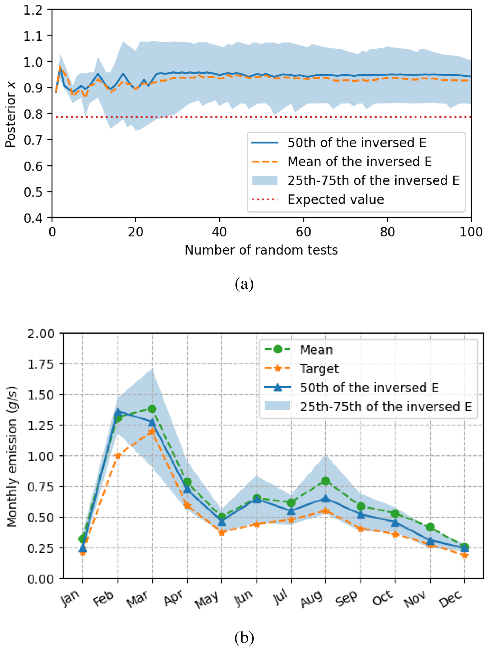
Figure 7 Results of yearly (a) and monthly (b) inversion of emission on Schiermonnikoog using synthetic observations. The results shown here correspond to the 2022 inversion.

The results in Fig. 7b present the monthly inversion performance for 2022. While the ensemble average appears reasonable, individual monthly inversions suffer from high uncertainty, primarily due to the limitations of the simulated MAN error. The passive sampling approach and associated errors are not well-suited for resolving finer temporal variability. As such, these findings highlight the need for higher-quality, high-resolution measurements to improve inversion accuracy at monthly scales and also reduce the impact of seasonal mismatches between model and measurements.

3.3 Inversion results of MAN

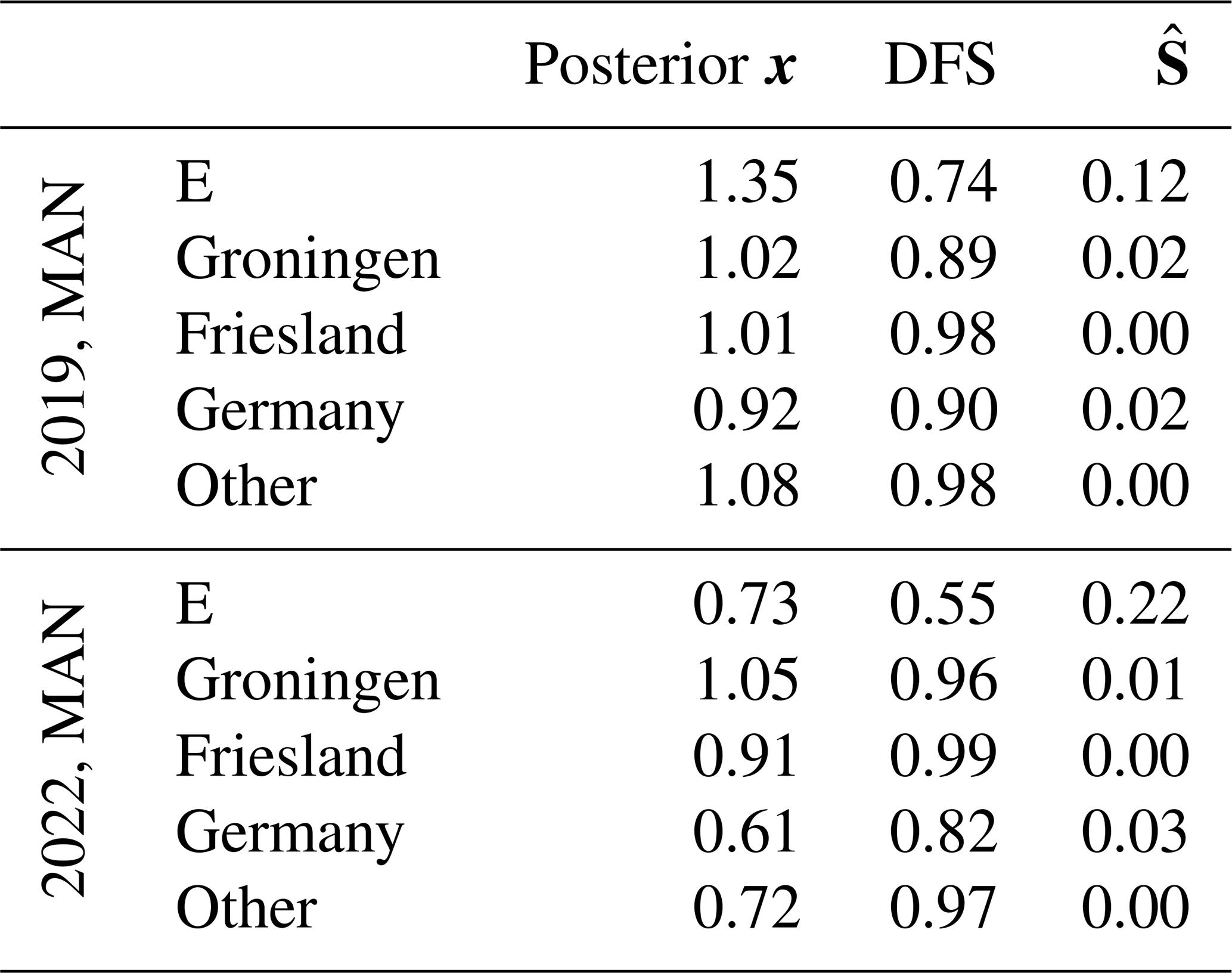
Table 3 presents the results of the ammonia emission inversion using MAN measurements for 2019 and 2022. The results show a notable reduction in total emission multipliers for Schiermonnikoog, from 1.35 (with a credible interval: 0.95–1.92) in 2019 to 0.73 (with a credible interval: 0.46–1.17) in 2022. Both inversions utilize the same 2019 emission inventory as prior. To reflect the uncertainty in the posterior estimates, the credible intervals are derived using the transformation ${\stackrel{\circ }{\mathit{x}}}_{\mathrm{post}}\cdot \left[\exp \left(-\sqrt{\widehat{s}}\right),\exp \left(\sqrt{\widehat{s}}\right)\right]$, as shown in Fig. 8. Despite the wide credible intervals, which is attributable to the sparse measurement network and high observational uncertainty, the inversion successfully captures both the direction and approximate magnitude of the emission reduction. These results indicate that the reduction in ammonia emissions on Schiermonnikoog is both detectable and significant. The monitoring system for the emission of Schiermonnikoog may still need to improve (due to a low DFS detected), but due to a larger region with a consideration of external influences, the results for the external influences received a larger DFS during inversion, indicating the fixation for the boundary condition is helpful.

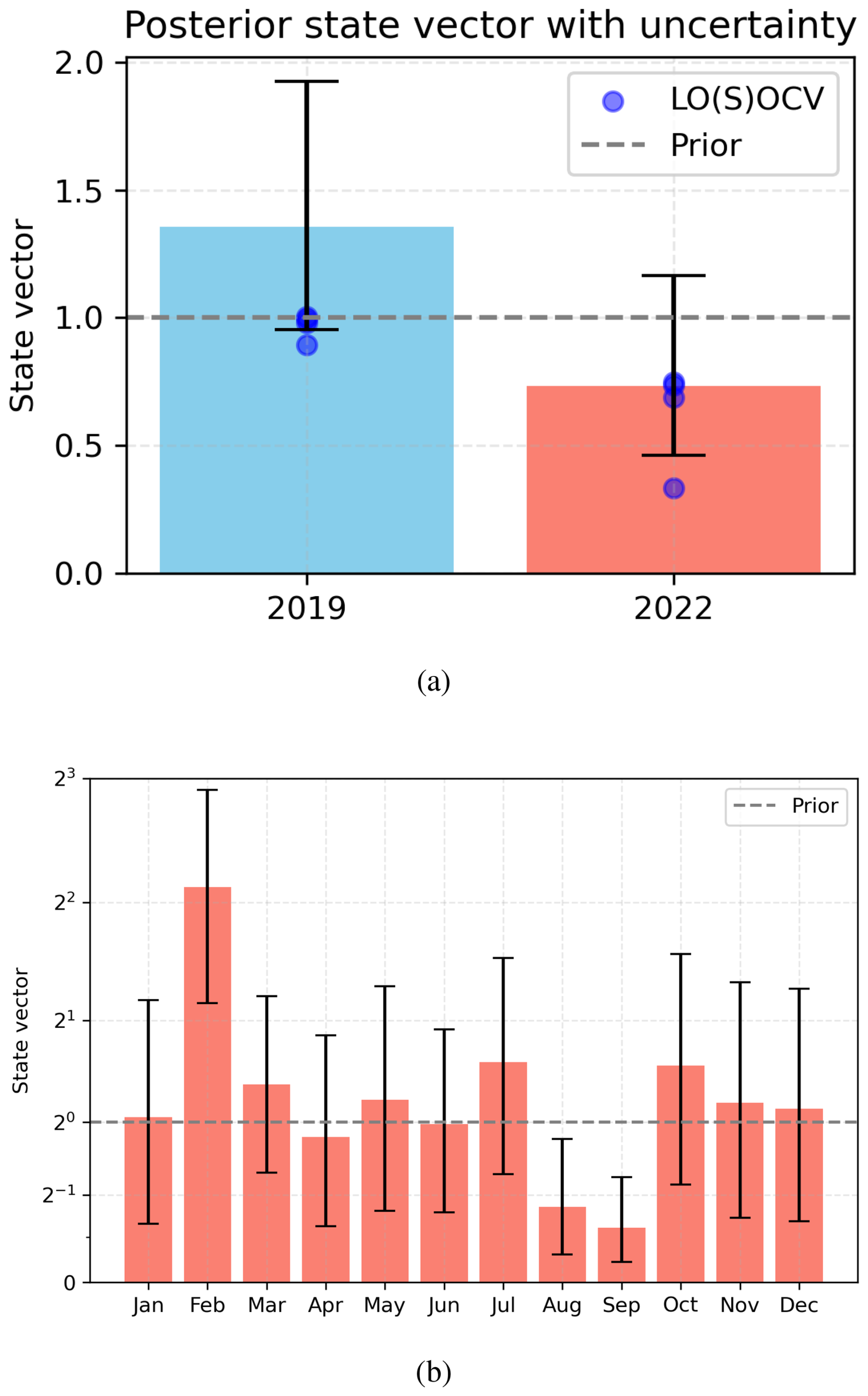
Figure 8 Results of MAN-derived yearly ammonia emission (a) and monthly ammonia emission (b) with the leave-one-source-out cross-validation (LOSOCV) and credible intervals, derived from the posterior error covariance matrix $\widehat{\mathbf{S}}$. The results shown in (b) correspond to the 2022 inversion.

The inversion results suggest a 51 % reduction in ammonia emissions on Schiermonnikoog between 2019 and 2022. However, this figure may be an overestimate. To address the concern, we performed a leave-one-source-out cross-validation (LOSOCV). This approach is analogous to leave-one-out cross-validation (LOOCV), but instead of omitting one measurement site, we iteratively exclude one state vector element that represents external influences. In each case, we subtract the correlated contribution and then re-conduct the inversion with the remaining elements. The posterior estimate for 2019 exceeded the range of the validation, although the credible interval still encompasses the validated values. This suggests that the apparent overestimation of the emission reduction originates primarily from an overestimation of the 2019 emissions rather than an underestimation in 2022. In contrast, the posterior for 2022 shows consistency with the validation and indicates a 27 % reduction compared with the prior emissions of 2019. Thus, the discrepancy between the inversion (51 % reduction) and the activity data (23 % reduction) can largely be attributed to uncertainties in the 2019 posterior emissions.

We also attempted to use the MAN measurements for monthly emission inversion (see Fig. 8b). However, the resulting posterior estimates exhibited high emission values during spring and notably low values in autumn. This asymmetry is caused by strong seasonal variability in both ammonia emissions and meteorological conditions. In spring, ammonia emissions increase and become more variable due to fertilizer application. Meteorological factors such as turbulence and boundary layer dynamics also contribute to greater atmospheric variability. Particularly, the posterior value of February exhibited more than four times the prior value, although the result falls within the leave-one-out cross-validation bounds (see Fig. S7). This increase likely reflects the onset of manure application season in February, when agricultural ammonia emissions typically peak due to fertilizer spreading on farmland. While both February and April fall within the spring period, in 2022, February experienced much stronger wind speeds (Fig. S5b), enhancing transport and dispersion. In contrast, April had lower wind speeds, which reduced the spread of ammonia and increased sensitivity to local sources. Additionally, in months like April, August, and September, prevailing north winds placed most observation sites on the leeward side of the source, reducing their sensitivity to local emissions and thus weakening the inversion constraint. In other words, the low results from the inversion may not be due to actually low emissions but rather to the measurements of those months that failed to capture and represent local emissions adequately. Additionally, the degrees of freedom for signal (DFS) remained low, indicating that the system could not extract sufficient information from the observations to reliably constrain the emissions.

In Sect. 3.4, we explore potential strategies to improve the performance of monthly emission inversions, including enhancements in measurement quality and network design.

Table 3 Inversion results of 2019 and 2022 with optimized observational error. The prior error covariances for the emission is 0.48 and for external influences are 0.16. Notably, the MAN data of July and August 2019 are eliminated because of the dune fires.

3.4 Optimizing the measurement network for evaluation of emissions

Due to the limitations of the current MAN network on Schiermonnikoog, the inversion is only sufficient for quantifying annual emissions, albeit suboptimally. Furthermore, these measurements exhibit high uncertainty, particularly in low-emission regions, making localized emission changes difficult to detect due to measurement noise. To address these challenges, we propose potential enhancements to the existing monitoring network to improve emission tracking on Schiermonnikoog.

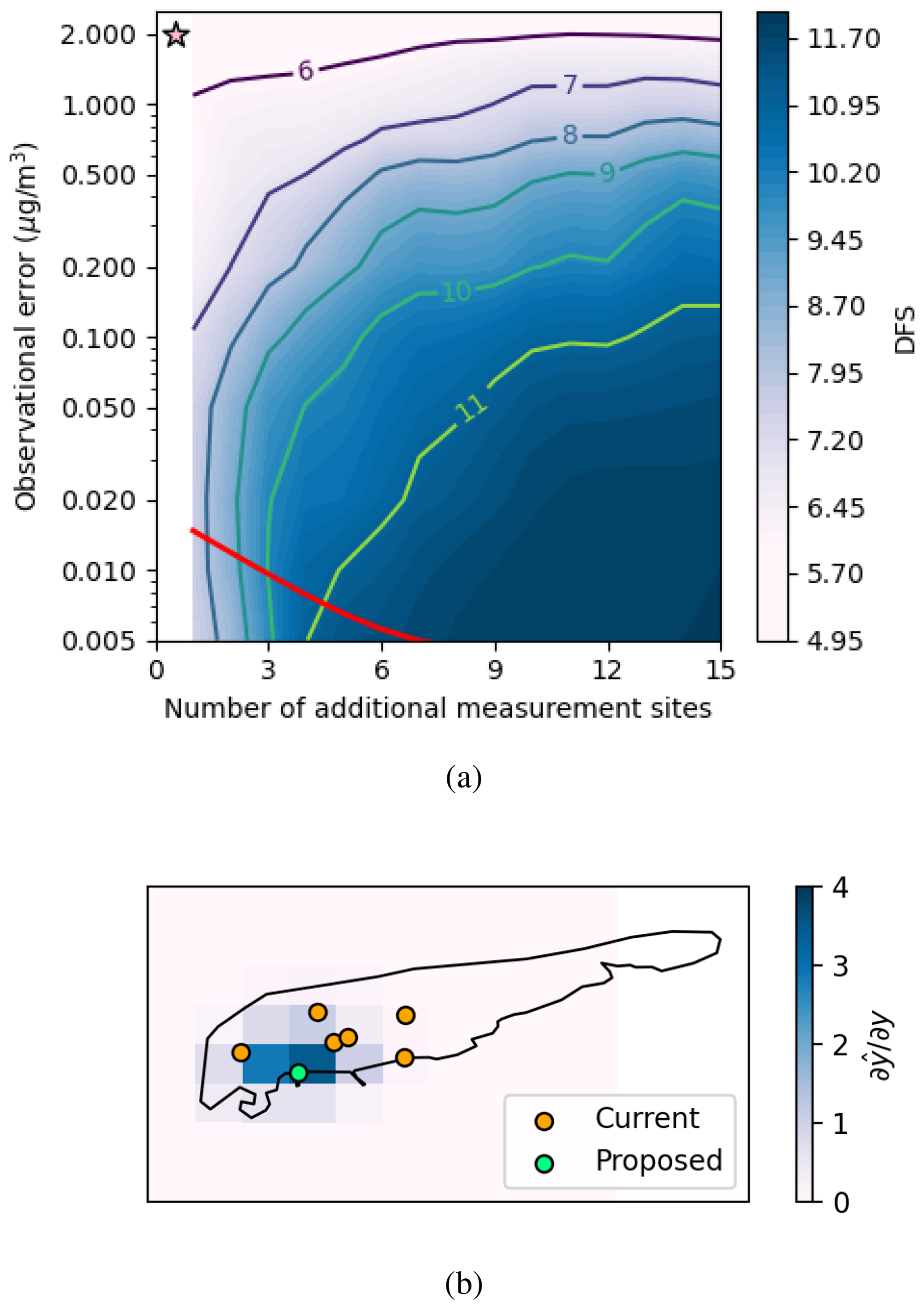
Figure 9 Panel (a) illustrates the DFS as a function of additional measurement sites and observational errors. The ridge line divides the plot into two regions: error-limited (above the ridge line) and site-limited (below the ridge line). Worth mentioning here, the measurement sites are added randomly; thus, (a) shows the averaged results. The star in (a) represents the current monitoring network. Panel (b) highlights the spatial distribution of observational usefulness. Assuming high-quality measurements are available across the entire island, we calculate the contribution of each observation to the inversion result; see Eq. (12) for details. This diagnostic provides insight into which locations offer the greatest information gain, thus informing the strategic placement of future monitoring sites. Circles show the current and proposed sites.

We apply a Monte Carlo approach to simulate Degrees of Freedom for Signal (DFS) under varying measurement network configurations. Specifically, we test the effects of increasing the number of monitoring sites across Schiermonnikoog and reducing observational errors to represent higher-quality measurements. Figure 9a shows the DFS results averaged over 20 randomized site configurations. The contour plot highlights how DFS evolves as a function of both site density and observational precision. The ridge line delineates the transition between two regimes: an error-limited regime (above the ridge), where measurement uncertainty dominates, and a site-limited regime (below the ridge), where sparse spatial coverage is the limiting factor. The results indicate that both increasing the number of sites and reducing observational errors can enhance DFS, but their relative effectiveness depends on the regime:

• in site-limited conditions, adding more sites leads to substantial DFS improvement;

• in error-limited conditions, further reducing observational uncertainty becomes more impactful.

The star in Fig. 9a marks the current MAN network configuration, which is constrained by relatively high observational errors, resulting in low DFS. While increasing the number of high-quality measurements would greatly improve the system, practical constraints such as cost and logistics make island-wide deployment of high-quality sensors difficult. This highlights the need for strategic placement of enhanced measurement sites to optimize inversion performance. Note that for denser monitoring networks (e.g., the bottom-right corner of Fig. 9a), the achievable improvement may eventually be limited by the ceiling of the model itself. In this case, part of the parameter space could be biased by model error, as also discussed in Turner et al. (2016). Nevertheless, for the current monitoring network, as well as for moderate improvements in measurement precision, the analysis still provides valuable insights.

Figure 9b displays the spatial distribution of observational usefulness across Schiermonnikoog, averaged over 100 random test realizations. Assuming that high-quality measurements (with an observational error of 0.1 µg m⁻³) are available uniformly across the island, we quantify the relative contribution of each observation to the inversion outcome using the following formulation (Rodgers, 2000):

$$\begin{array}{}\text{(12)}& {\displaystyle \frac{\partial \widehat{\mathit{y}}}{\partial \mathit{y}}}={\displaystyle \frac{\partial {\mathbf{K}}_N\widehat{\mathit{x}}}{\partial \mathit{y}}}={\mathbf{K}}_N\mathbf{G}\end{array}$$

where $\mathbf{G}=\widehat{\mathbf{S}}{\mathbf{K}}_N^T{\mathbf{S}}_{\mathrm{O}}^{-\mathrm{1}}$ is the gain matrix, $\widehat{\mathbf{S}}$ is the posterior error covariance, K_N is the Jacobian matrix at the final iteration, and S_O is the observational error covariance matrix. To quantify the influence of each observation only on the inversion of Schiermonnikoog emission, we take the first column and row of K_N and G, respectively, corresponding to the local agricultural emission component. The diagonal elements of this product reflect the influence of each observation on the inversion model outcome. These values are reprojected spatially in Fig. 9b. This diagnostic provides an intuitive interpretation of where observations are most impactful for the inversion. Regions with higher values indicate greater potential for improving the accuracy of emission estimates, offering a useful basis for strategic sensor placement in future monitoring network designs.

We then propose adding an LML-like measurement site near Waddenhaven Schiermonnikoog (53.472226° N, 6.167259° E), as shown in Fig. 9b. The most informative location would be directly at the island's main emission source. However, measurement close to the source can lead to a large bias in regional misrepresentation of ammonia concentration (Schulte et al., 2022). Waddenhaven offers a compromise: it is near the source but lies outside Banckspolder, a reclaimed polder valued for farming. In addition, all existing MAN sites are situated to the north of the source, which limits their effectiveness under northerly winds. By contrast, Waddenhaven lies within the footprint of the local emission and is typically downwind of the main source, making it the most suitable candidate for improving inversion performance.

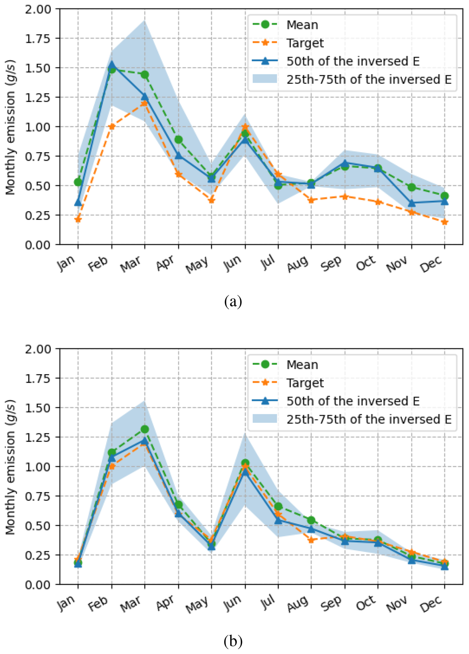
Figure 10 The monthly inversion in 2022 with synthetic measurements and a synthetic summer peak. The observational error for the synthetic LML-like measurement is set at 3.5 %. Panel (a) shows the posterior emission with the current MAN network. Panel (b) shows the posterior emission after adding one LML-like measurement.

Figure 10 illustrates the effect of incorporating a single high-quality, LML-like observation on monthly ammonia emission inversion for 2022. The synthetic observational error for the LML-like site is set at 3.5 %, based on values reported by Dammers (2017) and Blank (2001). Compared to the current MAN-only network, the addition of one strategically placed LML-like measurement significantly reduces uncertainty in most months. Posterior estimates not only align closely with target values but also exhibit a narrower percentile spread across most months, indicating improved stability. Overall, this result demonstrates that even a single, well-placed, high-precision observation can substantially improve inversion performance, enhancing the system's ability to track temporal variability and increase DFS. With high-frequency, low-error measurements, it becomes feasible to detect near-real-time emission changes.

In addition, observational error can be reduced by averaging multiple measurements at the same site, effectively decreasing the random component of the total error, as suggested by the central limit theorem. According to Noordijk et al. (2020) and Lolkema et al. (2015), the total monthly error in the MAN network comprises three components: random uncertainty, uncertainty from the calibration method, and systematic uncertainty from the calibration standard. The first two are random and can be substantially reduced by repeated sampling. By increasing the number of measurements at a given site and averaging them into a single “super-observation”, the total error can be significantly lowered, approaching the quality of high-precision instruments. While enhancing a single MAN site alone does not achieve the same performance as adding a single LML-like site, substituting all six MAN sites on Schiermonnikoog with corresponding super-observations yields substantial improvements. In fact, this approach performs even better than the LML-like configuration in March and April. More details are provided in the Supplement.

4 Conclusions

4.1 Summary

In this study, aiming to evaluate a documented emission reduction on the island of Schiermonnikoog in the Netherlands, we performed a local-scale Bayesian inversion of ammonia emissions using the LOTOS-EUROS chemical transport model as the forward model, with MAN (Measuring Ammonia in Nature) observations serving as constraints and CAMS-REG, GrETa, and ER inventories as prior estimates. To evaluate the influence of observational uncertainty, we performed sensitivity analyses by integrating residual errors with reported MAN network uncertainties from Lolkema et al. (2015) and Noordijk et al. (2020). By optimizing the χ² statistics, we derived observational error covariance matrices for both annual and monthly inversions, improving the robustness of the inversion framework.

Between 2019 and 2022, GVE (grazing livestock units) on Schiermonnikoog decreased from 639 to 541, with a particularly notable reduction in dairy cattle, corresponding to an estimated 23 % reduction in ammonia emissions based on activity data. Our inversion successfully captured this trend. Using the current MAN network, we were able to invert annual emissions, with the inversion indicating a 51 % reduction between 2019 and 2022. However, this value may be overestimated, largely attributed to uncertainties in the 2019 posterior emissions. Using the posterior error covariance, we derived a credible interval, describing the uncertainty of the inversion. The posterior for 2022 shows consistency with the validation and indicates a 27 % reduction compared with the prior emissions of 2019. In contrast, monthly inversions remain challenging with the current observational network. High measurement uncertainty hinders the system’s ability to resolve short-term emission dynamics effectively, especially for those months that failed to capture and represent local emissions adequately.

To explore potential improvements, we conducted sensitivity analyses of the Degrees of Freedom for Signal (DFS) and posterior error. Results showed that the existing network is limited by relatively high observational errors. Increasing the number of high-quality measurements substantially improves the inversion performance. In particular, adding a single, high-quality, LML-like observation at a strategically chosen downwind site, Waddenhaven, significantly enhanced the system's ability to resolve temporal variability and increased DFS.

4.2 Discussion

Although the model captures overall seasonal trends in both years, significant discrepancies remain in specific months, particularly during episodic events such as the dune fires in July and August 2019. Such events substantially affect local ammonia levels and underscore the need to include event-driven emissions in the modeling framework.

Furthermore, possible timing discrepancies in passive sampler collection, where measurements may not align precisely with calendar months, introduce additional uncertainty when comparing observations to model outputs. These issues highlight the need for refined emission timing, better spatial resolution, and improved observation methodologies to enhance simulation-observation agreement.

The source apportionment analysis revealed that ammonia concentrations on Schiermonnikoog are dominated by long-range transport, which makes emission reductions more difficult to detect due to the relatively high uncertainty in MAN measurements. However, the inversion results provide not only the emission changes but also an improved estimate of the transport contribution. While the model indicated that approximately 50 % of the ammonia originated from Germany, the posterior inversion suggests a lower contribution of about 30 %. Consequently, the local contribution is likely larger than indicated by the original source apportionment. In addition, the “Other” category, primarily representing ammonia re-emission through bi-directional flux processes, also plays a key role. This includes volatilization from both soil and sea surfaces. While LOTOS-EUROS can capture sea-air exchange processes, these remain highly uncertain due to complex atmospheric interactions and limited validation data over marine environments.

In this study we neglected off-diagonal terms in the observational error covariance matrix, effectively assuming errors are uncorrelated between sites. This assumption is supported by the dominance of random measurement errors and by the relatively small representation errors observed between nearby stations. Nevertheless, neglecting correlations means that potential systematic errors, such as seasonal biases in the model, are not explicitly accounted for. While this simplification is unlikely to strongly affect monthly inversions, correlated errors could become more relevant for annual-scale inversions.

4.3 Outlook

The findings from model evaluation and source attribution offer valuable insights for future ammonia inversion efforts. Persistent underestimation of summer ammonia concentrations suggests the need for improved temporal representation of agricultural practices, particularly manure spreading. Incorporating regional transport is also critical, as the island's ammonia concentrations are heavily influenced by upwind sources. Refining prior emission inventories with higher spatial and temporal resolution is essential for improving inversion outcomes. Deploying high-resolution, continuous measurements, such as LML-like instruments at strategically chosen sites, would provide much-needed constraints and enable more accurate inversion at finer timescales.

In conclusion, while LOTOS-EUROS demonstrates strong capability in capturing broad seasonal ammonia trends, it struggles with peak events and local-scale gradients. The source apportionment confirms that Schiermonnikoog's ammonia levels are mainly driven by regional transport, reinforcing the need for regional-scale mitigation strategies in addition to local emission reductions. This highlights the importance of coupling localized monitoring efforts with national and transboundary air quality policies.

Future work will expand the inversion domain to include broader regions and higher-intensity emission sources. Furthermore, since the current framework assumes a linear relationship between emissions and concentrations, we will explore non-linear Jacobian formulations, which may better capture the dynamics over diverse and complex emission landscapes. For upcoming national-scale inversion studies, we plan to first characterize emission patterns before applying inversion, to enhance both accuracy and computational efficiency. In addition, we will incorporate the potential influence of correlated errors when constructing observational error covariance matrices.