The historical climate trend resulted in changed vertical transport patterns in climate model simulations

Convective transport leads to a rapid vertical redistribution of tracers. This has a major influence on the composition of the upper troposphere (UT), a highly climate-sensitive region. It is not yet clear how the convective transport is affected by climate change. In this study, we applied a new tool, the so-called convective exchange matrix, in historical simulations with the chemistry–climate model EMAC (ECHAM/MESSy Atmospheric Chemistry) to investigate the trends in convective transport. The simulated deep convection is penetrating higher but occurs less frequently from 2011 to 2020 than from 1980 to 1989. The increase in the vertical extent of convection is highly correlated with a rise in the tropopause height. The upward transport of air mass increased on average to height levels of 130 hPa and above, but convection transported material less efficiently to the upper troposphere in general from 2011 to 2020 in comparison to the 1980s. These findings give rise to new opportunities to investigate long-term simulations performed by EMAC with regard to the effects of convective transport. Furthermore, they might provide a first insight into the trends in atmospheric convective transport due to changing atmospheric conditions and might serve as an estimate for the convective feedback to climate change.

1 Introduction

Moist convection plays a key role for the transport of heat and water in the Earth's atmosphere (Emanuel, 1994). Beyond that, deep convection is associated with extremely large vertical wind velocities. These lead to short vertical transport timescales and to a rapid redistribution of atmospheric tracers (Feichter and Crutzen, 1990). Consequently, convective transport has complex implications for the atmospheric composition and chemistry, especially in the upper troposphere (UT) (Mari et al., 2000; Lawrence et al., 2003; Bozem et al., 2017). As some studies argue, deep convection even influences the composition of the lower stratosphere (Ray et al., 2004; Tinney and Homeyer, 2021; Gordon et al., 2024) and could lead to a downward transport of ozone-rich air from the stratosphere to the UT (Frey et al., 2015).

It is highly important to capture convective transport and its effects (Barth et al., 2007). Many efforts were made towards a better representation of convective transport in models (Mahowald et al., 1995; Lawrence and Rasch, 2005; Tost et al., 2010; Li et al., 2018), a more comprehensive understanding of this process (Doherty et al., 2005; Lawrence and Salzmann, 2008; Bardakov et al., 2022), and the interplay of convective transport and the related scavenging of tracers (Mari et al., 2000; Barth et al., 2007; Bozem et al., 2017; Cuchiara et al., 2020, 2023).

Global warming affects atmospheric convection and might also influence convective transport. Lepore et al. (2021) found with the help of the Coupled Model Intercomparison Project Phase 6 (CMIP6; Eyring et al., 2016) simulation data that convective available potential energy (CAPE) increases in a warmer climate, likely causing an enhancement in severe storm frequency. Bolot et al. (2023) examined the changes in the ice water path in convective clouds due to temperature and CO₂ changes. The observed changes were closely linked to changes in the vertical upward velocities within convective clouds (Bolot et al., 2023). Del Genio et al. (2007) already detected an increase in the updraft velocity performing simulations with doubled CO₂ concentrations. The effect of warming on the updraft intensity was also confirmed by Singh and O'Gorman (2015). In the case of a change in either convection occurrence or strength (or both), it can be assumed that the corresponding convective transport will be modified as well.

Stevenson et al. (2005) performed a 40-year projection to investigate the trends in tropospheric ozone concentrations under climate warming conditions. Within this simulation, the tropical convection occurs less frequently in the 2020s compared to the 1990s, but the updrafts strengthened at about 150 hPa, which influences the vertical transport. The work by Stevenson et al. (2005) highlights the importance of investigating the adaptations of convective transport to understand the response of the climate system to warming. However, so far, it is not fully clear how convective transport processes change in detail and to what extent. Therefore, our study follows up with the question: how does climate change specifically influence the convective transport? How has the transport efficiency and extent of the updraft, the downdraft, and the balancing subsidence changed with time?

This article addresses this question by performing historical simulations with the chemistry–climate model EMAC (ECHAM/MESSy Atmospheric Chemistry, Jöckel et al., 2006, 2010, 2016) using the convective transport scheme ConVective tracer TRANSport (CVTRANS) by Tost et al. (2010). To do so, we added a new feature to analyse convective transport, namely the convective exchange matrix similar to the mixing matrix by Bechtold (2017). This new tool connects convective transport from all possible starting levels to all possible destination levels in a model when utilising a convection parameterisation. This enables a deeper understanding of the changing transport processes and their causes. The goal of this study is to investigate the changes in deep convective transport towards the UT over the past decades.

This study is structured as follows: the global chemistry climate model EMAC and submodel CVTRANS are briefly described in Sect. 2. In the same section, the convective exchange matrix is introduced before the simulation setup is described. In Sect. 3, we analyse the results, focusing on the changes in transport over the past decades. The implications, the significance, and the limitations are discussed in Sect. 4. The summary and the outlook are given in Sect. 5.

2 Model description

2.1 EMAC

The global chemistry and climate model EMAC (Jöckel et al., 2006, 2010, 2016) consists of the general circulation model European Centre Hamburg general circulation model version 5 (ECHAM5; Roeckner et al., 2006) and the Modular Earth Submodel System (MESSy; Jöckel et al., 2005, 2006, 2010, 2016). MESSy is a software framework to couple different submodels with a chosen base model and includes a steadily growing number of these submodels. For example, Vella et al. (2023) used EMAC recently to combine a global dynamic vegetation model with an atmospheric model. In this study, MESSy version 2.55 is used to link the submodel CVTRANS (Tost et al., 2010) with ECHAM. The dynamic representation of convection is given by the Tiedtke–Nordeng convection scheme (Tiedtke, 1989; Nordeng, 1994), as implemented in the CONVECT submodel within the MESSy structure (Tost et al., 2006).

2.2 CVTRANS

The submodel ConVective tracer TRANSport (CVTRANS) was introduced by Tost et al. (2010) to account for convective tracer transport in EMAC. This submodel can reproduce observed changes in the vertical profiles of non-soluble tracers due to convection sufficiently well (Tost et al., 2010). It makes use of a single plume/bulk convective transport parameterisation based on the formulation of Lawrence and Rasch (2005). Tost et al. (2010) applied the convective mass fluxes for the updraft, downdraft, entrainment, and detrainment from the convection parameterisation to calculate the redistribution of the tracers. The mass fluxes must fulfil the following equations,

$$\begin{array}{}\text{(1a)}& {\displaystyle }{F}_{\mathrm{u}}^k=F_{\mathrm{u}}^{k+\mathrm{1}}+E_{\mathrm{u}}^k+D_{\mathrm{u}}^k\text{(1b)}& {\displaystyle }{F}_{\mathrm{d}}^{k+\mathrm{1}}=F_{\mathrm{d}}^k+E_{\mathrm{d}}^k+D_{\mathrm{d}}^k,\end{array}$$

as described by Tost et al. (2010). F refers to the mass fluxes, D refers to the detrainment, and E refers to the entrainment. The subscripts _u and _d denote the updraft and the downdraft. k indicates the model level. If this relation is not satisfied, the detrainment or entrainment should be adapted accordingly (Tost et al., 2010).

Strong updrafts can lead to mass balance problems; i.e. more mass is transported out of a model box as mass is transported into the box within one time step. The mass fluxes are rescaled to prevent a mass imbalance in such cases. This procedure can lead to a damping of the convective transport. To overcome this issue, Ouwersloot et al. (2015) included intermediate time stepping in CVTRANS to ensure optimum handling of intense convective events.

Note that the transport of water vapour and hydrometeors is not considered in the convective tracer transport algorithm, as the convection parameterisation itself takes care of the redistribution of water species. Some adjustments to CVTRANS were included to increase the physical consistency compared to Tost et al. (2010); however, these changes do not affect the results of this study substantially (further information can be found in the Supplement).

2.3 Description of the convective exchange matrix

CVTRANS directly calculates the new tracer profiles. Therefore, it is difficult to analyse the convective transport itself due to the impact of the various background profiles. The convective exchange matrix overcomes this issue. This new tool in EMAC makes use of the same basic principles as the mixing matrix which was introduced by Bechtold (2017). Firstly, in every vertical model level ($\mathrm{1},\mathrm{2},\mathrm{\dots },N$), one pseudo-tracer (${\mathit{P}}_{\mathrm{1}},{\mathit{P}}_{\mathrm{2}},\mathrm{\dots },{\mathit{P}}_N$) is initialised with a value of 1 kg m⁻². N denotes the number of model levels. By definition, the vertical model level with the highest number, level N, is closest to the surface. In all other levels, the pseudo-tracers are set equal to zero. The vertical profiles of the pseudo-tracers can be written as N-dimensional vectors. Applying this, the pseudo-tracer P₁ is given by ${\mathit{P}}_{\mathrm{1}}=(\mathrm{1},\mathrm{0},\mathrm{0},\mathrm{\dots },\mathrm{0})$, and P₂ is ${\mathit{P}}_{\mathrm{2}}=(\mathrm{0},\mathrm{1},\mathrm{0},\mathrm{\dots },\mathrm{0})$. Putting all these vectors together results in an N×N diagonal matrix, as can be seen on the left side of Fig. 1a.

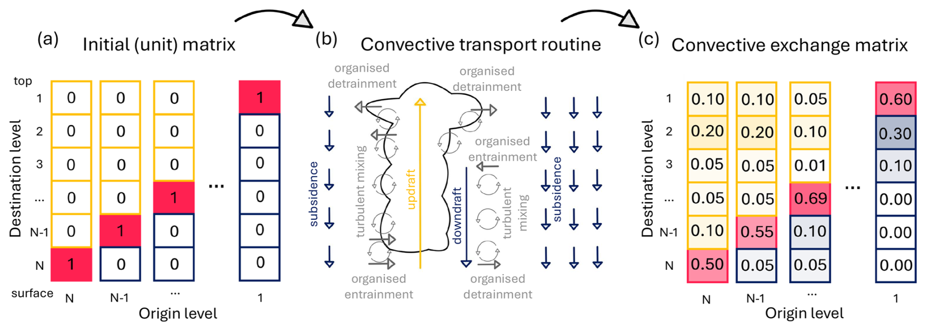
Figure 1 Sketch of the principle behind the convective exchange matrix. Panel (a) shows the input matrix. Panel (b) illustrates the convective transport processes. The yellow arrow indicates the updraft, the blue ones indicate the downdraft and the mass-balancing subsidence, and the grey ones indicate the organised and turbulent detrainment and entrainment. The redistribution is calculated with the transport routine within the submodule CVTRANS. Panel (c) shows an example of a convective exchange matrix: it is only for illustration and is not a case calculated during a simulation. In both matrices, the reddish fields denote the main diagonal. The yellow fields show the matrix entries influenced by the updraft, and the blue fields denote the matrix entries affected by the downdraft and the grid-scale subsidence. Synoptic-scale processes are not considered.

The time integration, i.e. the vertical redistribution by convective transport of the pseudo-tracer field, is performed based on the transport routine in CVTRANS (Tost et al., 2010) for the convective exchange matrix. The considered processes are shown in Fig. 1b. The time integration results in the convective exchange matrix (TrMa). The entries of the matrix give the portion of the air mass (m_air) that was transported from a specific departure level (given by the pseudo-tracer field in the beginning) to a certain destination level. For example, TrMa_i,j with $i,j=\mathrm{1},\mathrm{\dots },N$ describes how much m_air was transported from level i to level j. If j=i, then TrMa_i,i characterises the contribution of level i to level i itself. In other words, it shows the amount of air that was not affected during the convective event. This is illustrated in Fig. 1c and highlighted in red. The upper-left entries (yellow in Fig. 1) represent the transport from a level i to level j with i>j, i.e. the upward transport to level j which started in level i. Thereby, the notation is that the lowest model level has the highest number and the uppermost level is level 1. The downward transport (transport from a lower-level number to a higher-level number in this notation) is marked in blue in Fig. 1c. An example of a convective exchange matrix can be found in the Supplement for one event (see Fig. S1b).

Figure 2 shows how the convective transport matrix is structured (a) in the tropics and (b) in the mid-latitudes. Again, the highest model level number (31) refers to the level closest to the surface/the level with the highest pressure. This is the case for the destination and origin levels. Roughly the following characteristics of convective upward motion (yellow in Fig. 2) are visible in the convective exchange matrix:

1. Shallow convection and turbulent detainment, when the origin level is located in the boundary layer (BL) and the destination level is also located in the BL or in the lower troposphere.

2. Deep convective updrafts make it to the upper troposphere originating in the BL.

3. Some deep convective events even reach the height of the tropopause and beyond (upper-left corner in Fig. 2a and b).

4. Upward transport also starts in free-tropospheric levels and in UT levels mainly due to turbulent entrainment into the updrafts.

The downward motion is shown in blue in Fig. 2. The mass balancing subsidence is especially visible in the adjacent diagonals below the main diagonal. The subsidence can reach further towards lower pressure, the stronger the convective event is. The outflow of the downdraft is located in the BL levels. The difference between the tropics and the mid-latitudes is that the convective exchange matrix is compressed in the mid-latitudes, figuratively speaking (compare Fig. 2a and b). The tropopause is located at higher pressures (higher model level numbers) in the mid-latitudes compared to tropical regions.

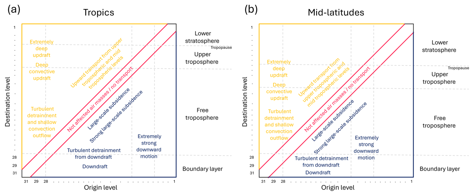
Figure 2 The convective exchange matrix is illustrated, including areas which roughly reflect specific transport mechanisms. This sketch can be used as an interpretation assistance of the convective exchange matrix. Panel (a) shows the convective exchange matrix with regard to the tropics, and panel shows it (b) with regard to the mid-latitudes. The colour code is as in Fig. 1.

The redistributed concentrations of trace species can be calculated with the convective exchange matrix by a simple matrix multiplication of the TrMa with the vertical tracer mixing ratio profile, as now implemented in the new version of CVTRANS (CVTRANS v3.0). For a large number of tracers (∼ 100 tracers), the computational efficiency is similar when the convective exchange matrix is applied to calculate the new concentrations of the tracers after the convective transport instead of using the transport algorithm itself. Consequently, for a higher number of tracers, this new algorithm can become computationally more efficient. The advantage of the convective exchange matrix is that the effects of the tracer transport can be studied disentangled from the specific background profiles of the tracers. Thus, it can be investigated, e.g. where the maximum outflow height is located and how much air mass can be transported upward inside a whole model grid cell at a specific height. The contribution to a certain destination level can also be calculated for all starting levels. This can be helpful to track a measured air mass containing tracers backward and to investigate how strongly it was affected by convection in its air mass history.

2.4 Simulation setup

Three-dimensional global simulations have been conducted with the convective exchange matrix implemented utilising EMAC. A total of 31 vertical pressure levels up to 10 hPa are used, and a horizontal resolution of T63 (triangular truncation with wavenumber 63) has been applied. This is associated with 192 × 96 grid points with areas between 32.5 km × 32.5 km in the polar regions and 207.9 km × 207.9 km in the tropics and a time step of 12 min. Temperature, vorticity, divergence, and surface pressure are nudged towards ECMWF reanalysis fifth generation (ERA5; Hersbach et al., 2020) and the sea surface temperature and the sea ice coverage are prescribed by the nudging data. The nudging is based on Jeuken et al. (1996) and applied as described by Jöckel et al. (2006).

An overview of all submodels used is given in the Supplement (Table S1). The essential ones for this study are mentioned in the following. A basic methane chemistry is applied to take the water vapour production in the stratosphere and its influence on radiation into account using the submodel CH4 (Winterstein and Jöckel, 2021). Further considerations of chemical reactions are not necessary, because this study exclusively investigates the redistribution of air masses by convection and not the effect on single tracers. Monthly mean values for greenhouse gases are used to include their radiative effect based on Jöckel et al. (2016). The Tanre et al. (1984) climatology is used for tropospheric aerosol as described by Jöckel et al. (2016). For the stratospheric aerosol radiative effect, optical properties of the chemistry–climate model initiative (CCMI) database (Revell et al., 2017) are applied, e.g. as in Jöckel et al. (2016). The submodel CONVECT by Tost et al. (2006) is applied with the Tiedtke–Nordeng scheme to calculate the parameterised convective properties needed in CVTRANS to calculate the convective exchange matrix.

3 Results

We performed nudged EMAC simulations applying the convective exchange matrix from January 1979 to December 2020. For reducing spin-up and initialisation effects, the first year is discarded, such that the convective properties and the convective transport are analysed for the period from 1980 to 2020. This time period is sufficient to give a first impression of the climate response of the modelled convective transport. The analysis is only performed between 60° S and 60° N because this is the area where convection is of high relevance.

We point out that the transport is discussed referring mainly to model levels and not pressure levels because the pressure varies largely between the boxes mainly due to orography and secondary due to weather systems. A re-gridding is not possible in a convincing manner, as interpolation artefacts would violate the mass balance. We try to refer to specific areas in the atmosphere as boundary layer, free troposphere, upper troposphere, and lower stratosphere for a better understanding, but these also depend on the orography and the latitude. The reader is referred to Table S2 to get an impression of the tropopause height and the boundary layer height in the model. The equivalent pressure is presented alongside the model levels to allow a rough estimation of the pressure. This equivalent vertical pressure is based on a vertical profile where the pressure in the box closest to the surface is 1013 hPa.

3.1 Global changes

The convective transport matrix is shown in Fig. 3 for the temporal mean of the 10-year period 2011 to 2020 and the area-weighted mean between 60° N and 60° S. The mean transport matrix is shaped by a large number of initial unit matrices because atmospheric moist convection is a rather localised effect. As a consequence, the mean convective transport is not as intense on a global scale as for an individual local deep event (compare Fig. S1b). Nevertheless, the convective transport has a non-negligible effect on large spatial and temporal scales.

The strongest upward transport can be seen in Fig. 3 starting in the lower free troposphere and in the BL (level 31 to 26) and reaching only into the lower free troposphere (level 29 to 25), representing shallow convection and turbulent detrainment from updrafts. Deep upward transport starts mostly in the same heights (levels 31 to 28) but shows lower fractions than the transport into the lower free troposphere. Starting levels in the free troposphere are associated with lower portions of upward-transported material. The mass-balancing subsidence is the dominant downward transport mechanism over two to three levels below the main diagonal. From the lower- to mid-tropospheric-origin levels, the downdrafts transport air mass especially to the three levels closest to the surface.

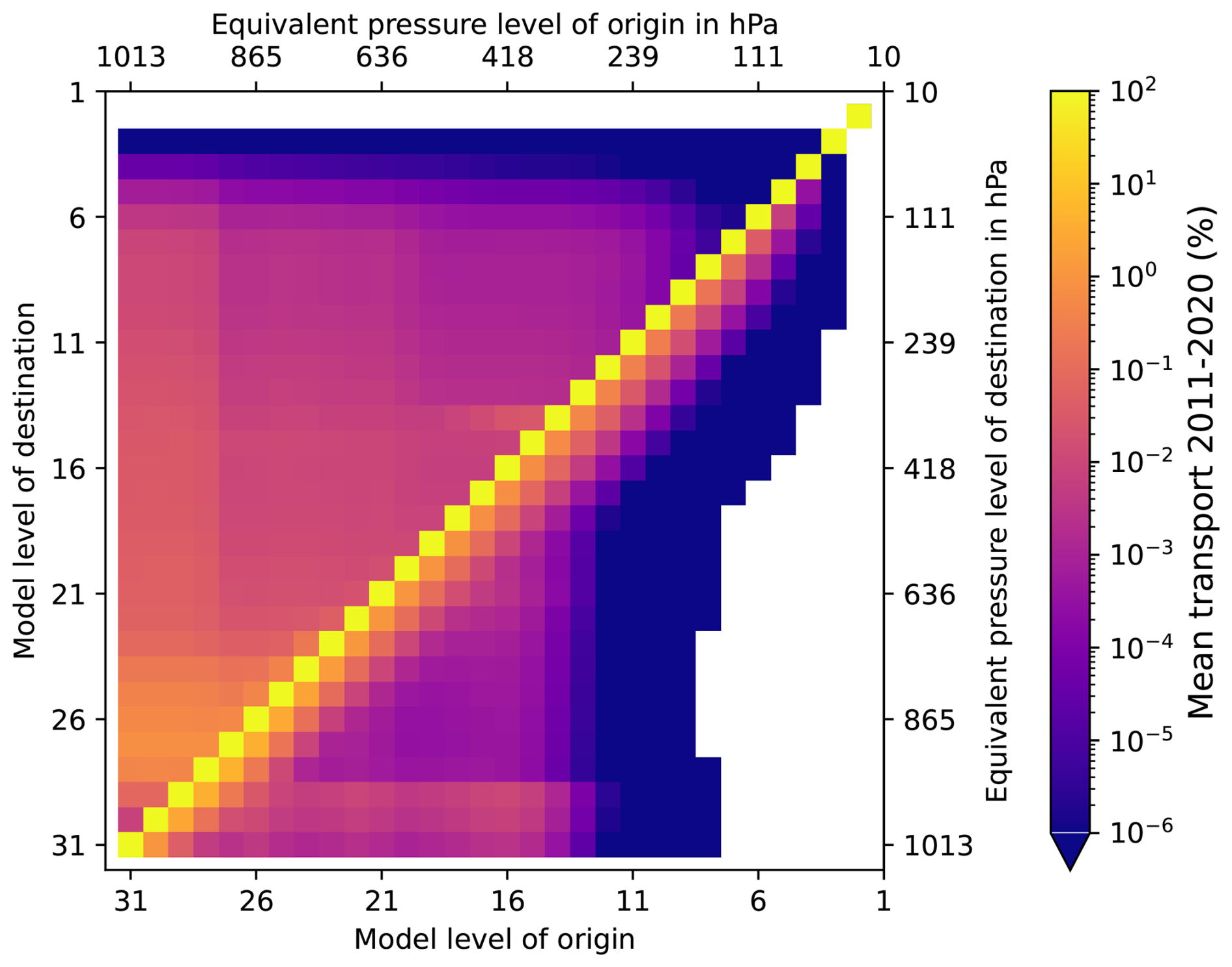
Figure 3 Area weighted between 60° N and 60° S and temporal mean convective transport matrix, i.e. the fraction of air mass which was transported from an origin to a source level, for 2011 to 2020. Note that the equivalent pressure (upper and right axis) is determined from a standard atmosphere over the ocean with zero orography.

Figure 4 shows the temporal and spatial mean convective transport compared between 2011 and 2020 to the reference period from 1980 to 1989. The transport to levels with low pressures (level 4 to 7) increased significantly from all starting levels below the destination levels. The subsidence adapted accordingly. More material descents from levels which are associated with the upper troposphere in the tropics and with the upper troposphere and lower stratosphere in the mid-latitudes (between level 12 and 4).

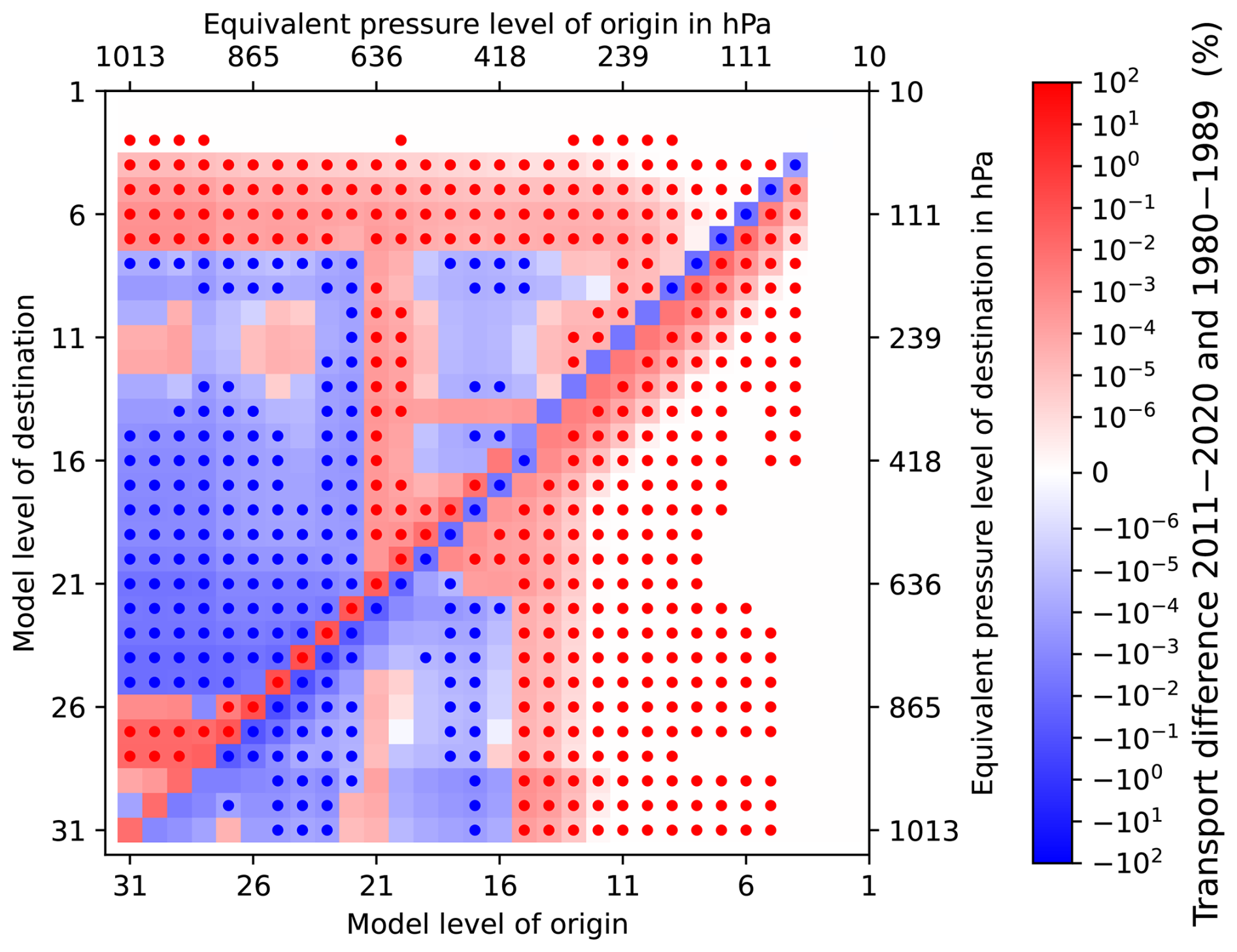
Figure 4 Changes in the convective mean transport between 60° S and 60° N. The temporal (10-year) and global (area-weighted) convective exchange matrix is compared from 2011 to 2020 and from 1980 to 1989. Red areas denote that the values were higher in the period 2011 to 2020, and blue areas show that the entry in the convective exchange matrix was higher from 1980 to 1989. A dot in a box indicates statistical significance. A two-sided Student's t test was used with a significance threshold of 1 % for every side of the t distribution.

These features of the difference convective exchange matrix (Fig. 4) can be explained considering the frequency distributions of the updraft mass fluxes compared for the reference time period and 2011 to 2020 (Fig. 5). In Fig. 5, the mass fluxes from deep convective events were categorised according to their strength. The lowest class (below 1 × 10⁻⁷ kg m⁻² s⁻¹) contains all no-events, so the cases where no deep convection occurred or the mass fluxes were too small. The class with the strongest updraft mass fluxes contains all mass fluxes which are stronger than 0.2 kg m⁻² s⁻¹. This classification was performed for all height levels. The difference of these mass flux distributions is shown in Fig. 5 for a selected set of model levels and for the values from 2011 to 2020 minus the ones from 1980 to 1989. For a better visualisation, the symmetric logarithmic difference is shown instead of the absolute numbers. The updraft mass flux in the upper levels (height range of the tropopause) shifts to stronger mass fluxes in the later time period. Moreover, more events reached these levels from 2011 to 2020 in comparison to the reference period. This trend is consistent with the increased transport to the upper level as observed in Fig. 4.

The enhanced transport to levels roughly associated with the tropical tropopause could be explained by an increase in the strength of the convection or even an enhancement of convection overshooting the tropopause. A non-significant tendency towards more overshooting convection is predicted by the Tiedtke–Nordeng scheme over the 41-year time period. We define one (tropopause) overshooting event as an event when the updraft mass flux associated with one convective event reaches beyond the independently calculated tropopause in one column and at the same time step. It cannot be ruled out that the detected overshooting is only an artefact of the coarse model resolution because both the tropopause height and the mass flux are mean values. It can be assumed that both quantities vary significantly within a box. However, the latter does not affect the convective transport in the model because the transport only sees the grid box mean values. Wu et al. (2023) discovered that tropical convection reaching beyond the tropical cold-point tropopause occurred slightly more often in the future scenario (2075–2104, Intergovernmental Panel on Climate Change A1B emission scenario) than in their historical simulations (1979–2008). Concerning this study, the trend in tropopause overshooting convection is not significant. Therefore, it can be ruled out as a primary source for the major increased convective transport to the tropical tropopause/lower stratosphere levels (level 7 to 4).

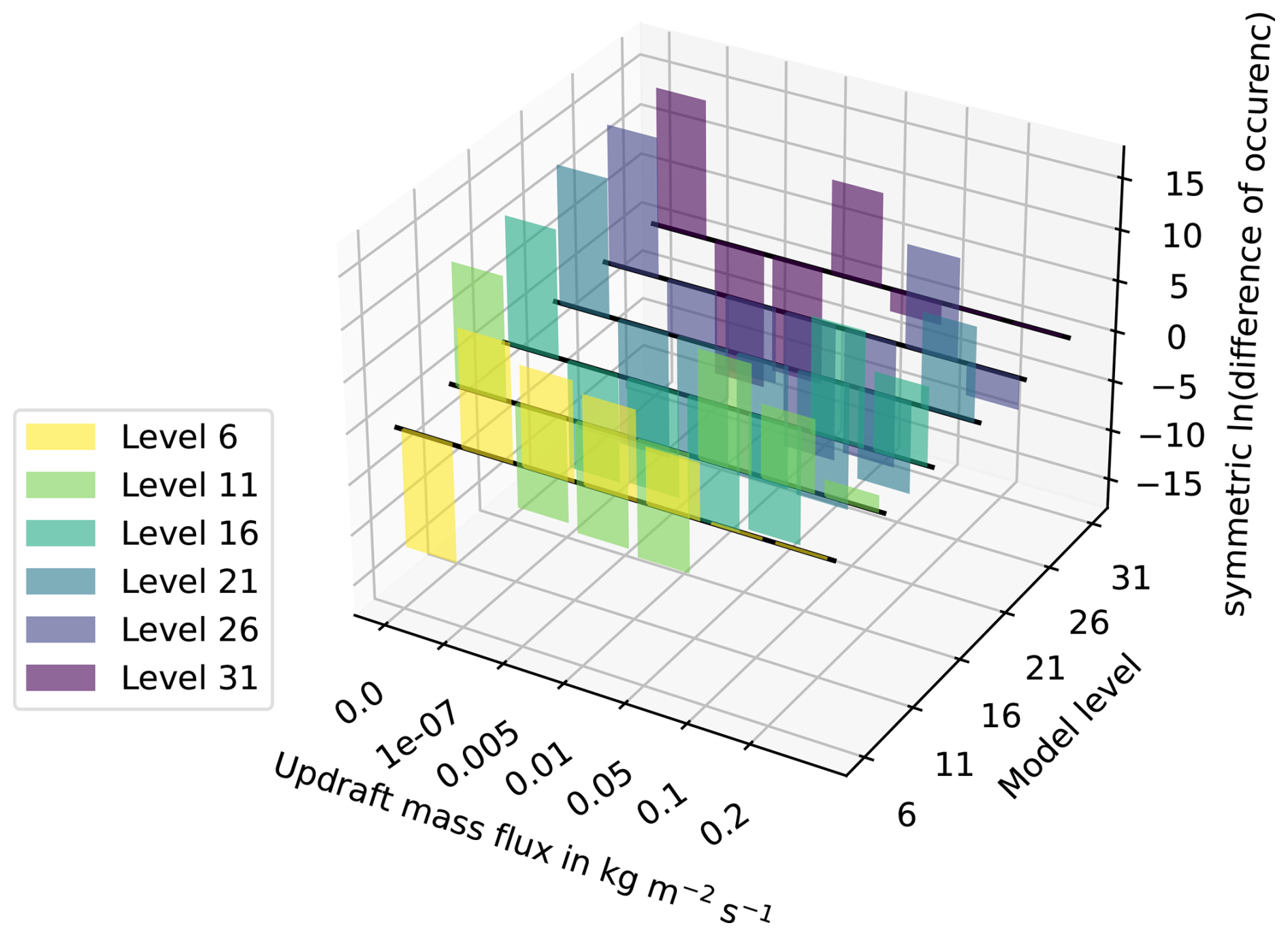
Figure 5 The distribution of the updraft mass fluxes is given as the symmetric logarithmic difference between the absolute frequency distributions from 2011 to 2020 minus the one from 1980 to 1989. The colours denote different altitude levels. Updraft mass fluxes are divided into seven categories. Updraft mass fluxes below 1 × 10⁻⁷ kg m⁻² s⁻¹ are not considered in the transport routine CVTRANS. Therefore, these mass fluxes are in the smallest category and are considered to be no occurrence of convection.

The model predicts a rise in the global mean tropopause (not shown). A higher troposphere could clear the path for convection with a larger vertical extent, but an increased penetration of convection could also cause a lifting of the tropopause height (for the second possibility, see Gettelman et al., 2002). Deep convection tends to occur less frequently (Fig. 6), and, for this reason, the increased height of the deep convection can have a rather local impact on the tropopause height. Therefore, we assume that the dominating process is the change in tropopause height, which leads to deeper convection and not vice versa.

The upward transport has decreased from starting levels in the lower troposphere (levels between 31 and roughly 21) to the destination levels in the mid-troposphere and some upper troposphere in the most recent time period in comparison to the 1980s (see Fig. 4). Figure 5 is considered again to examine possible reasons for this decrease in upward transport. Deep updraft convective mass fluxes occurred less frequently in many height levels with relevant values (larger 1 × 10⁻⁷ kg m⁻² s⁻¹) from 2011 to 2020 in comparison to the 1980s. A bimodal trend emerges from Fig. 5 in terms of the changes in the distribution of the deep updraft mass fluxes. The mass fluxes tend to be either at the stronger edge or zero in the later time period. Higher mass fluxes are generally favoured in the uppermost levels in the later period, shown in Fig. 5 (level 6). Therefore, the negative trend in some upper-tropospheric levels in Fig. 4 can be attributed to an increase in the outflow height and a decreasing trend in the occurrence of deep convective events over the 41-year period (Fig. 6).

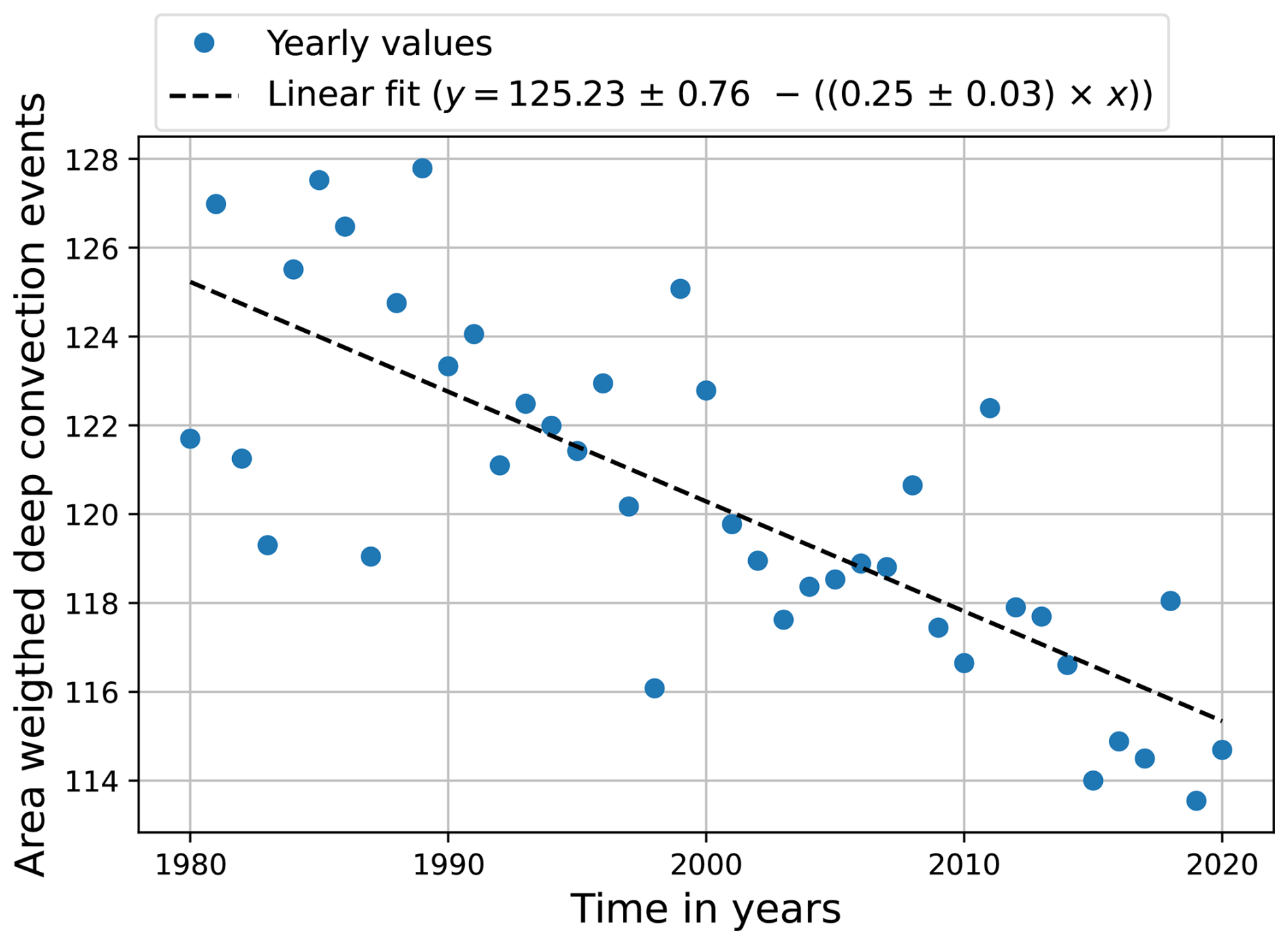
Figure 6 Normalised time development of the area-weighted deep convection events per year. The blue circles denote the yearly number of convective events, and the dashed line is the linear fit of the area-weighted deep convection events. x denotes the number of relative years; thus, x is equal to zero for 1980. The standard error of the slope and the intercept are given for the linear fit. y is the number of area-weighted deep convective events per year.

The upward transport increased for two starting levels in the mid-troposphere (levels 20 and 21) on average from 2011 to 2020 compared to the reference period depicted in Fig. 4. This leads to the hypothesis that mid-level convection occurred more frequently; however, mid-level convection according to the definition in the Tiedtke–Nordeng scheme did not increase in number (not shown). On the other hand, shallow updraft mass fluxes show higher values in the two mentioned mid-tropospheric levels (levels 20 and 21). The same is the case for the mid-level convection. However, the mid-level convection headed towards a more frequent occurrence of the higher mass fluxes for a wide range of altitude levels. These could play a role in this prominent increase in upward transport from these two mid-tropospheric levels (level 21 and 20), but the reason for this cannot be unambiguously clarified at this point.

The downdrafts shift to starting levels located higher above the surface in the later time period compared to the reference period (Fig. 4). The impact of downdrafts starting at the mid- to upper troposphere (levels 15 to 13) has increased; i.e. more mass is transported downward from mid-tropospheric levels. On the other hand, the downward motion is reduced for origin levels in the free to mid-troposphere (between 26 and 16) on average from 2011 to 2020. This finding goes well along with the height increase in the deep convective systems.

A strengthening of the updraft detrainment is observed in Fig. 4 in the lower troposphere (up to level 26). This could be due to an increase in shallow convection because of the water vapour and lapse rate feedback on convection (e.g. Dagan et al., 2018, and references therein). However, the global occurrence of shallow convection did not significantly increase during the 41-year period (not shown). This means that either the shallow convection intensifies or the detrainment of mid-level and/or deep convection must increase.

In summary, more material stays at its original level for levels in the BL to mid-troposphere. This trend is significant for many mid-tropospheric levels (between levels 27 and 17). This also points towards an overall reduced deep convective transport.

3.2 Tropical and extra-tropical trends

Figure 7a shows the difference convective exchange matrix for 30° N to 30° S. Overall, the changes in tropical convective transport match well with the ones for the global case (Fig. 4). The convective transport increased to levels up to the tropical tropopause (level 7 and above) from 2011 to 2020 in comparison to the 1980s. The downdrafts also shift to starting levels located further up with regard to the surface, and more mass balancing subsidence is found for the upper-tropospheric to lower-stratospheric levels. In total, more material stays at the starting level and is not affected by the convection for a substantial number of levels. There is only one dissimilarity between the tropical and the global case: the significance of convective transport differences compared to the reference period in the BL (level 31 to 29) increased.

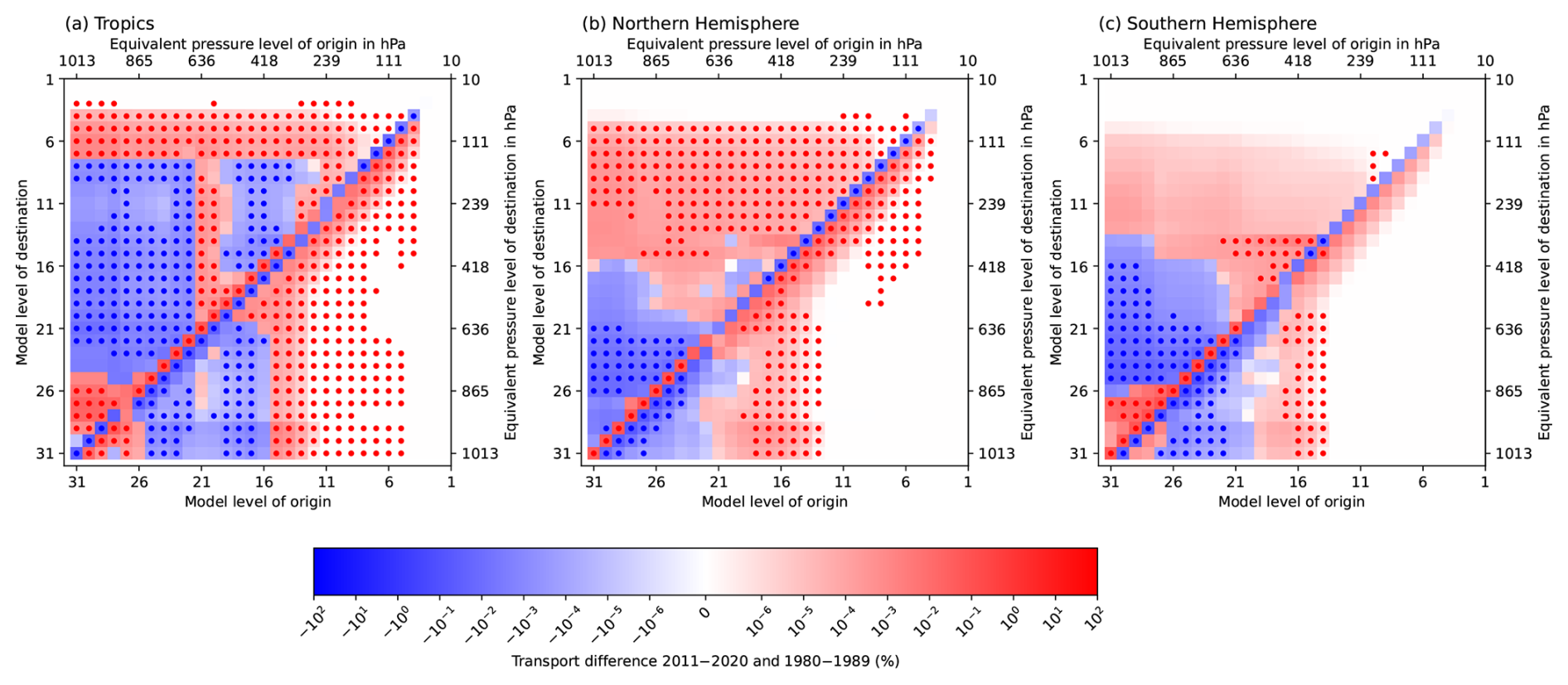
Figure 7 Changes in the convective mean transport in different regions. Same as Fig. 4 but (a) for 30° S to 30° N, (b) for 60 to 30° N, and (c) for 60 to 30° S.

The picture arising for the Northern and Southern Hemisphere extra-tropics seems to alter from the tropical one (Fig. 7b and c compared with Fig. 7a). The upward transport is pronounced for a wide range of levels. The tropopause is located mostly at higher pressures in the extra-tropics than in the tropics (Fig. 2 and Table S2). Considering the differences in tropopause height, the main patterns in convective transport changes are similar in all considered regions compared to the latest 10 years of the simulation with the 1980s: (1) the convective transport to the tropopause region and above is increased. (2) The mass balancing subsidence strengthened from origin levels at about the tropopause height/lower stratosphere. (3) The downdrafts originate at higher levels. (4) Less material from the boundary layer/lower troposphere reaches the free to upper troposphere (up to level ∼ 16). Thereby, the convective transport changes are not often as significant and as much pronounced in the Southern Hemisphere compared to the Northern Hemisphere.

3.3 Regional differences

The mean convective transport from the boundary layer to the upper troposphere is calculated for each grid column to assess the regional variability in convective transport. The UT is heuristically defined as the region vertically ranging from the tropopause level (in Pa) down to the level where the pressure is equal to the tropopause pressure plus 150 hPa. The tropopause height and the height of the planetary boundary layer are taken from the EMAC output.

The mean upward transport is not directly comparable to a tracer concentration in the UT or tracer release studies as performed by Levine et al. (2007), Hoyle et al. (2011), or Wang et al. (2021). Transport by the updraft interplays with the grid-scale subsidence, grid-scale advection, and other processes which lead to a combined impact on the transport of a tracer. The convective exchange matrix opens the possibility to study the upward transport driven by convection undisturbed by other processes and pre-existing tracer distributions. In this section, the focus is on the regional differences and “trends” in the upward transport from the BL to the UT.

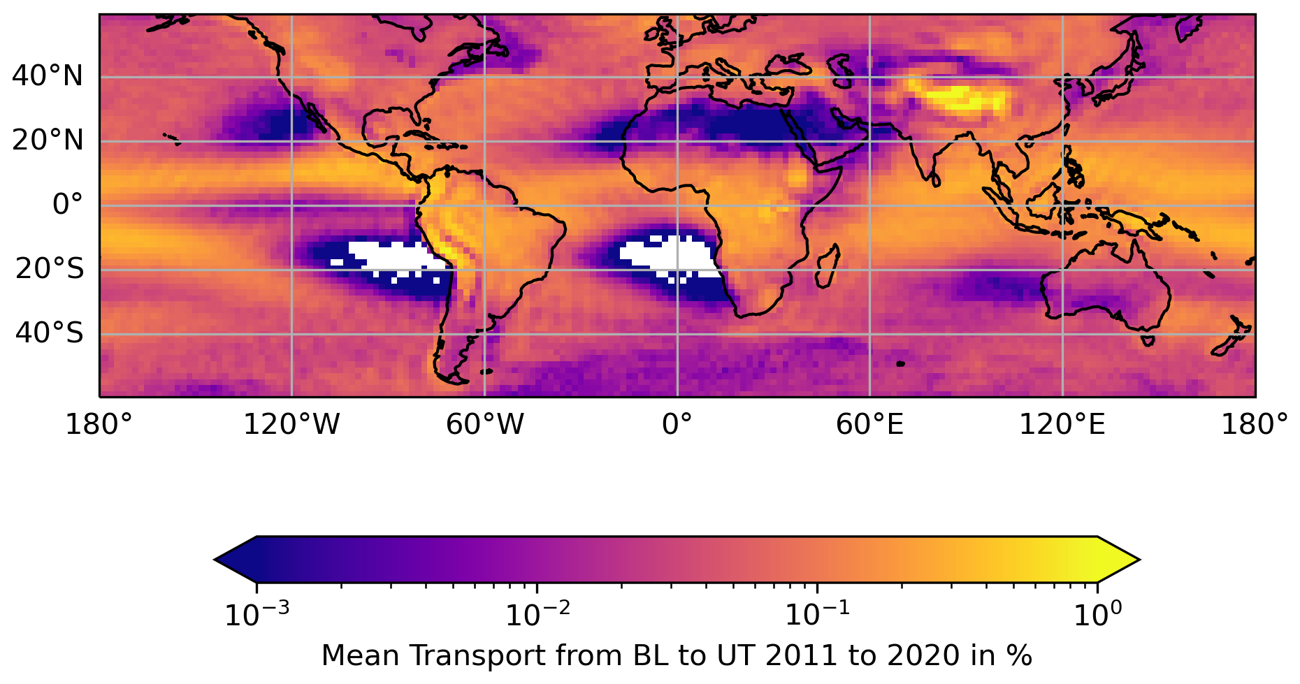
Figure 8 10-year-mean (2011 to 2020) convective mean transport from the planetary boundary layer height to UT within 12 min. The UT is defined as the vertical region between the tropopause and the height of tropopause in Pa plus 150 hPa.

The 10-year mean of the BL-to-UT transport (Fig. 8) shows a similar structure to the convective precipitation (compare Adler et al., 2017, and Sun et al., 2018, their Fig. 8) and the cloud top brightness temperature (compare Gettelman et al., 2002). The values are enhanced in the inner tropical convergence zone, Amazonia, central Africa, and the North Atlantic storm track. Particularly high portions of air mass were transported from the BL to the UT above the Himalayas and the northern to the central Andes mountains. This is not surprising for two reasons: (1) the model levels are compressed above high mountain areas. Thus, the distance between the BL and the UT is reduced. (2) It can be assumed that the Tiedtke–Nordeng scheme does not perform sufficiently well in these areas in general because the precipitation rates calculated with the Tiedtke–Nordeng convection parameterisation within EMAC are too high compared to observations in these areas, as shown by Tost et al. (2006) in their Fig. 2. As the freshly formed precipitation is proportional to the updraft mass flux, an updraft mass flux that is too strong results in an overestimation both of the convective precipitation and of the convective upward mass transport. No air masses were transported from the BL to the UT west of Africa and South America at about 20° S (with areas in Fig. 8), where subsidence is dominating the large-scale circulation patterns. Small but non-zero values indicate very low (deep) convective activity west of Australia, over northern Africa, and off the coast of California (dark areas in Fig. 8).

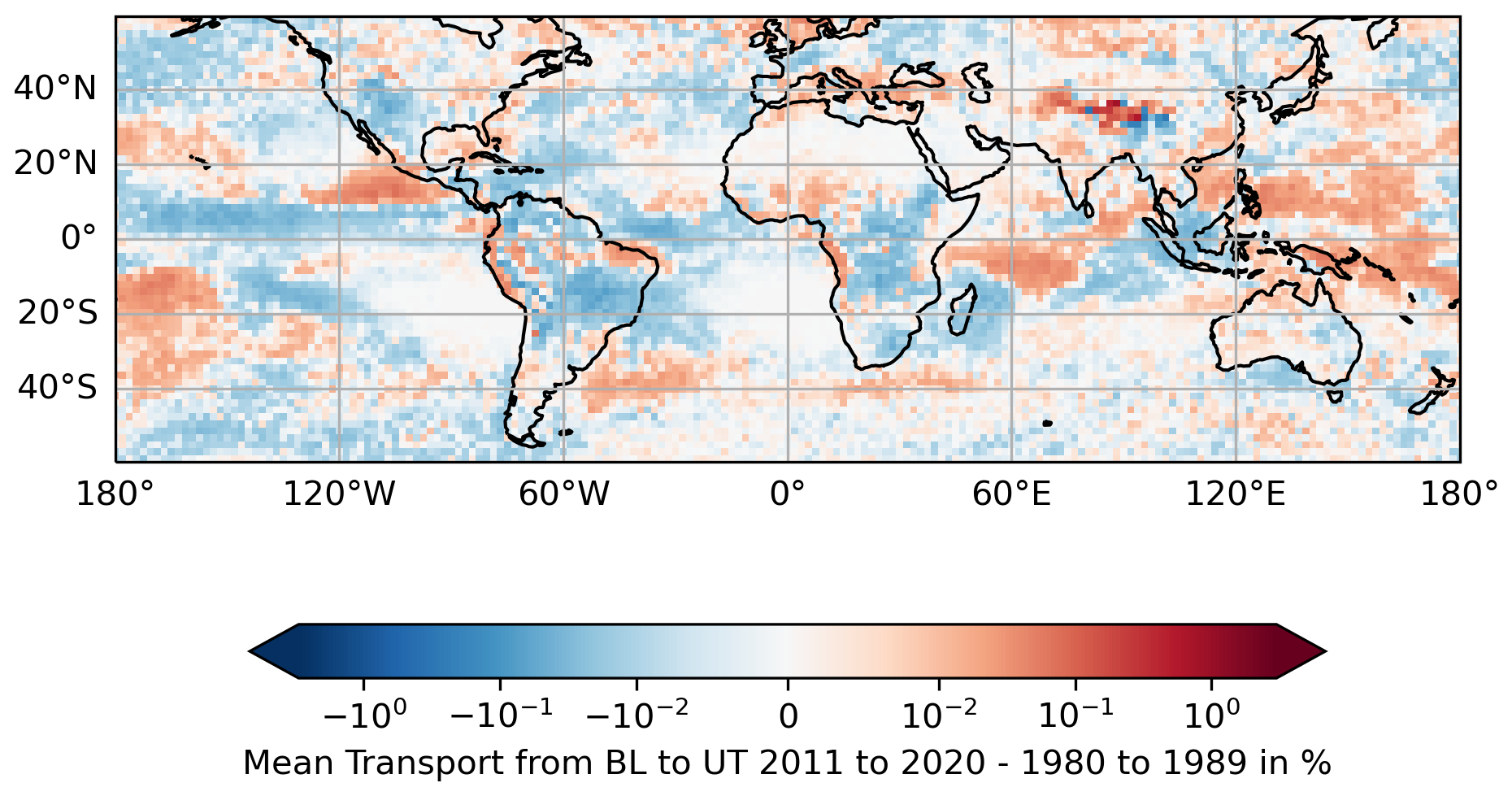
Figure 9 As in Fig. 8 but for the difference in the mean values of 2011 to 2020 and 1980 to 1989.

The change in the mean BL-to-UT transport is characterised by regional differences (see Fig. 9). In dependence of the region, the trend is either negative or positive. Overall, the transport from BL to UT was only slightly smaller between 2011 and 2020 than in the reference period. The global (60° S to 60° N) area-weighted average decreased from 0.07909 % per time step (1980 to 1989) to 0.07829 % per time step (2011 to 2020). This seems counter-intuitive at first glance because of the significant increase in transported air masses to the upper levels of the convective exchange matrix (compare Fig. 4). First and foremost, the increase in the convective outflow height leads to the increased transport to the uppermost levels influenced by the convection (levels 4 to 7) (in Fig. 4), likely due to an increase in the tropopause height. This does not necessarily imply an increased transport into the whole UT.

The mean transport from the BL to the tropopause region remains nearly unchanged. Thereby, the region of the tropopause is defined as the level of the tropopause down to the level with a pressure equal to the pressure at the tropopause plus 50 hPa (in contrast to the UT, which was defined by the tropopause pressure +150 hPa). The mean transported portion was 0.02114 % per time step in the reference period and increased marginally to 0.02118 % per time step from 2011 to 2020. This indicates that less convection reaches the UT in general but that the convective transport to the tropopause region stays similar due to compensating processes: the deeper penetration balances or even exceeds the effect due to the lower occurrence rate of deep convection. We note that these trends are rather small and need to be validated in the future.

The transport to the UT decreases close to the Equator over the Central and Eastern Pacific. North and partly south of this area (at ∼ 20° N and ∼ 20° S), an increase in transport becomes apparent compared to the reference period. A possible weakening and widening of the Hadley cell (Lu et al., 2007; Hu et al., 2018) could explain this trend. In this framework, we cannot confirm or reject this hypothesis.

The problems of the underlying convection parameterisation are an important factor for the convective transport as well. The regions with the largest changes are widely the areas of the least accurate simulations of precipitation by the Tiedtke–Nordeng convection scheme. This convection parameterisation overestimates the precipitation at the Pacific coast of Central America, central Africa, the western Pacific Ocean, and the western Indian Ocean and underestimates the precipitation over the western Maritime Continent, as can be seen in Fig. 2 by Tost et al. (2006). These areas show pronounced changes in the transport of BL air to the UT. These changes, therefore, go along with high uncertainties, which we cannot further quantify due to a lack of global observations of convective transport or mass fluxes.

3.4 Natural variability in convective transport

To analyse whether the regional changes originate from climate change or are due to natural variability, one La Niña event (Fig. S4) is compared with one El Niño event (Fig. S5). For the El Niño event, 1 July 1982 to 30 June 1983 was chosen because Ren et al. (2018) identified it as an extreme event. According to Ren et al. (2018), a strong La Niña event took place in 1988 and 1989, and this is chosen because the conditions are very different from the El Niño event. For consistency reasons, we took the second half of 1988 and the first half of 1989 for the La Niña case into account.

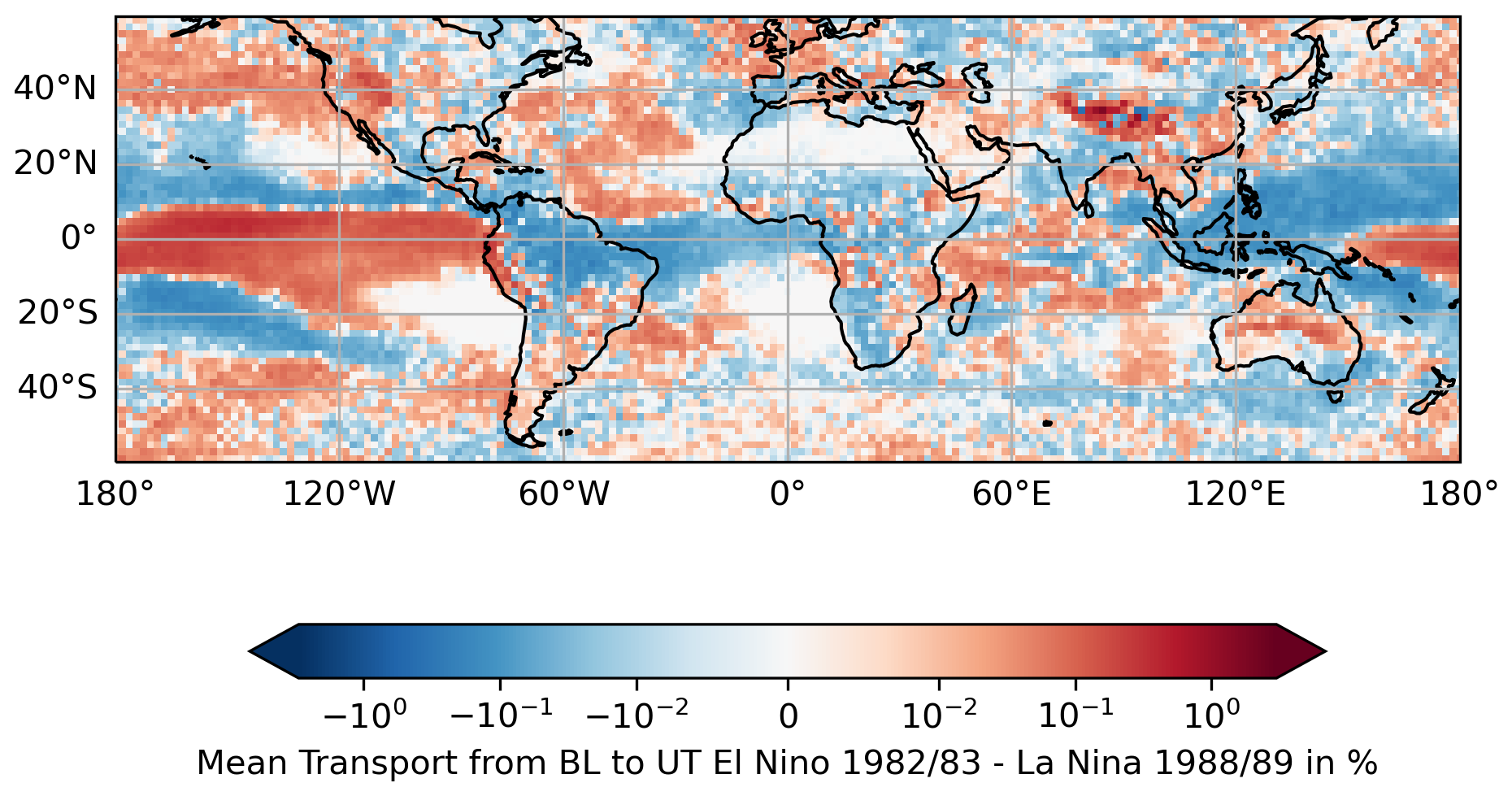
Figure 10 As in Fig. 8 but for the difference between the El Niño event 1982/83 and the La Niña event 1988/89.

The largest differences between the El Niño and La Niña events occurred in the area of the Equator over the Pacific. The mean transport to the UT from the BL differs up to 0.38 % per time step (Fig. 10). Sullivan et al. (2019) found an increased number of organised convective events in the same area comparing El Niño events with La Niña events between mid-1983 and mid-2008. This matches with the presented results from this study, that there is more transport into the UT from the BL during the considered El Niño event. A huge decrease can be observed northwards and southwards from the Equator in the Pacific (∼ 20° N and ∼ 20° S) and over the Maritime Continent (0°) when comparing the El Niño event from 1982/83 with the La Niña event from 1988/89 (Fig. 10). Overall, the differences between the El Niño event and the La Niña event are much more pronounced than changes in Fig. 9.

4 Discussion

In Sect. 3.1, a rather small sample size is used to identify changes in convective activity due to climate change. We investigated the periods from 1990 to 1999 and from 2000 to 2009 and compared them to the reference period (Figs. S2 and S3) to further substantiate the discussed changes in the redistribution of air masses. The differences in the convective transport patterns are not as significant when comparing 1990 and 1999 to the 1980s but are qualitatively alike to Fig. 4. The similarity to Fig. 4 is even more evident for the period from 2000 to 2009 compared with the reference period. Therefore, the trend is consistent over the decades and strengthens when the climate change signal intensifies. However, the temporal changes in the mean BL-to-UT transport are small on a regional scale in comparison to the maximal inner decadal variability induced by El Niño and La Niña events. Further uncertainties arise from the use of a convection parameterisation. Moreover, the results might depend on the choice of the convection parameterisation because the convective transport of individual events depends on the convection scheme (Tost et al., 2010). Therefore, this analysis can provide a first hint but no reliable information about the convective transport outside the model framework of EMAC with the Tiedtke–Nordeng convection scheme.

The nudging can introduce uncertainties as well because the ERA5 data already include convective processes. This might lead to less unstable conditions and might influence the triggering of convection in the model. This process was investigated in further detail by Schneider (2018). Schneider (2018) also discussed that nudging affects the tropopause height. We cannot avoid these issues because nudging is necessary to perform a transient simulation as close as possible to the real world or at least to the reanalysis. To test the robustness of our results, we performed another simulation with a comparable setup, but nudging was only applied for the surface pressure. Nevertheless, neither the trend of the tropopause height nor the trends concerning the mean convective transport change qualitatively.

Our results are to some extent consistent with other studies. An increase in the tropopause height/a decrease in the tropopause pressure has already been determined in several studies, for example, via radiosonde observations for the tropics by Seidel et al. (2001) and for the Northern Hemisphere by Meng et al. (2021), via reanalysis data by Wilcox et al. (2012) and Weyland et al. (2025) (only for the Northern Hemisphere), and by performing a multi-model inter-comparison (Gettelman et al., 2010). Based on satellite data, Richardson et al. (2022) and Raghuraman et al. (2024) observed a rise in the height of high clouds in the tropics which aligns with the deeper convection we determined. Also, Muller et al. (2011) concluded from simulations that convection penetrates deeper with higher sea surface temperatures.

Taszarek et al. (2021) discovered a wide-ranging decreasing trend in thunderstorm environments based on ERA5 data. Their calculated severe thunderstorm hours show a decrease for the mid-latitudes but partly an increase in the tropics. On the other hand, Lepore et al. (2021) found an increasing trend for severe storms across various regions using proxies based on CMIP6 projections. Del Genio et al. (2007) found that the updraft speed can strengthen up to 1 m s⁻¹ due to a CO₂ increase by a factor of 2. Our simulations suggest a bimodal trend favouring no convective updrafts at all or strong updraft mass fluxes (Fig. 5) from 2011 to 2020 compared to 1980 to 1989. Del Genio et al. (2007) state that the updraft speed increased the most in the UT. This is in good agreement with our finding that the deep updraft mass fluxes become stronger in the UT from 2011 to 2020 than in the reference time period. Stevenson et al. (2005) found in climate projections from 1990 to 2030 that tropical deep convection will reach higher and occur less often. The hindcast simulations from this study confirm these results for the tropics. Also, Gettelman et al. (2002) obtained a strong correlation between the deepest convection and the highest tropopause altitudes.

5 Conclusions

We investigated the changes in convective transport due to climate change by applying the submodel CVTRANS, which handles the convective tracer transport in EMAC and can reproduce measured profiles of insoluble tracers (Tost et al., 2010). We implemented a new feature, the convective exchange matrix, into CVTRANS. It is similar to the mixing matrix by Bechtold (2017) and opens the path for a new analysis approach for convective transport by directly connecting the convective inflow and outflow levels within EMAC. Thereby, the investigation of convective transport can be completely disentangled from other processes. With this new feature of CVTRANS, transient EMAC simulations have been performed for a 42-year period.

The convective transport reaches higher altitudes mainly due to an increase in the tropopause height. The upward transport increased to a wide range of upper-tropospheric to lower-stratospheric levels in the extra-tropics, where the tropopause height shows substantial variability. However, the changes in the convective transport patterns are, in general, similar to those in the tropics. Less material is transported upward from the BL to levels associated with the free troposphere. This indicates that the convective transport is reduced in the extra-tropics in total. The same is the case in the tropics. Globally, the mean transport is also weaker from the BL to the UT from 2011 to 2020 compared to the reference period. The simulations revealed a trend in decreasing occurrence of deep convection. Overall, this leads to less frequent but more penetrative convection, which is in line with the results of Stevenson et al. (2005).

The regional trends are accompanied by great uncertainties. The extreme events associated with El Niño and La Niña lead to a large variability within 1 decade. This makes it hard to identify anthropogenically generated changes on a local scale. Lepore et al. (2021) had the same issue for the historical time period and determined stronger signals using projections. Therefore, it might be promising to test how the convective transport will adapt to climate projections. Moreover, the choice of convection parameterisation is a source of uncertainty that should be considered. More complex and comprehensive convection parameterisations exist nowadays. An overview of the developments can be found in Rio et al. (2019). For this reason, we plan to extend this study and investigate the impact of different convection parameterisations in the past and projected climate.