CH₄ emissions from Northern Europe wetlands: compared data assimilation approaches

Atmospheric inverse modelling and ecosystem data assimilation are two complementary approaches to estimate CH₄ emissions. The inverse approach infers emission estimates from observed atmospheric CH₄ mixing ratio, which provide robust large scale constraints on total methane emissions, but with poor spatial and process resolution. On the other hand, in the ecosystem data assimilation approach, the fit of an ecosystem model (e.g. a Dynamic Global Vegetation Model, DGVM) to eddy-covariance (EC) flux measurements is used to optimize model parameters, leading to more realistic emission estimates.

Coupled data assimilation frameworks capable of assimilating both atmospheric and ecosystem observations have been shown to work for estimating CO₂ emissions, however ecosystem data assimilation for estimation CH₄ emissions is relatively new. Kallingal et al. (2024a) developed the GRaB-AM data assimilation system, which performs a parameter optimization of the LPJ-GUESS against eddy-covariance estimation of CH₄ emissions. The optimization improves the fit to EC data, but the validity of the estimate at large scale remained to be tested.

In this study, we confronted CH₄ emissions optimized using the GRaB-AM system to atmospheric CH₄ observations and to emission estimates from the LUMIA regional atmospheric inversion system (Monteil and Scholze, 2021). We found that the two approaches lead to very consistent corrections to the prior emission estimate from natural wetlands, with roughly a halving of the annual total compared to the LPJ-GUESS prior. Our findings confirm the interest of the GRaB-AM approach to constrain the contribution of natural ecosystems to the total methane budget, which is difficult to achieve for atmospheric inversions outside regions where emissions from natural ecosystems clearly dominate the emission budget.

1 Introduction

Methane (CH₄) is the second most important greenhouse gas after CO₂, accounting for around 21 % of the total effective radiative forcing of the well-mixed greenhouse gases (Forster et al., 2023). Its presence in the atmosphere has more than doubled since pre-industrialization era, with background mixing ratio at Mauna-Loa approaching the 2000 ppb (1931.91 ppbv in April 2024, according to https://gml.noaa.gov/ccgg/trends_ch4 (last access: September 2024). After a stabilization from 1998 to 2007, the atmospheric CH₄ concentration has started increasing again, at an accelerating pace. Although several recent studies attribute this renewed increase mainly to anthropogenic emissions (Nisbet et al., 2016; Thanwerdas et al., 2024), an important contribution from wetlands has also been proposed (Qu et al., 2022; Peng et al., 2022; Christensen, 2024). While for the global natural methane budget, tropical wetlands are most important, Arctic wetlands could constitute a potent positive climate feedback (Zhang et al., 2023) and there are indications that their emissions have been increasing in recent years (Yuan et al., 2024; Ward et al., 2024).

Emission estimates for natural wetlands can be obtained through process models, which calculate methane emissions according to various environmental inputs (meteorological forcings, soil type, hydrology, etc.). The model simulates or approximates known physical processes with various degrees of complexity. However, uncertainties on the existence or the importance of specific processes, lack of accuracy of some parameterizations, combined with the high non-linearity of the models leads to large differences between the estimates at large scales. For example, a comparison of mean annual CH₄ emissions from 16 models used in the Global Carbon Project (GCP) has shown that global estimates range from 118.7 to 195 Tg CH₄ yr⁻¹ (Ito et al., 2023). Specifically for wetlands above 15° N, the estimated emissions ranged between 10.5 Tg CH₄ yr⁻¹ (SDGVM model) and 40 Tg CH₄ yr⁻¹ (ORCHIDEE). Similar ranges were also found during the WETCHIMP model intercomparison project (Melton et al., 2013), which reported a ±40 % spread of the estimates around the all-model mean of 190 Tg CH₄ yr⁻¹, for global emissions.

The Global Rao-Blackwellized Adaptive Metropolis (GRaB-AM) approach developed by Kallingal et al. (2024a) is a parameter estimation data assimilation system based on Bayesian statistics, in which parameters of the LPJ-GUESS model connected to the production, transport and oxidation of CH₄ pathways are adjusted to optimize the model fit to eddy-covariance flux measurements. The optimized parameters can then be used to produce a gridded estimate of the methane emissions, which combine the process knowledge embedded in the LPJ-GUESS model with the added information from in-situ flux observations. However, the quality of the resulting emission estimate remains difficult to formally assess. The optimization is done by performing site-scale simulations, with local measurements of meteorological forcings and a good knowledge of the wetland types and their spatial distribution. Scaling up to Northern hemispheric emissions is then done using forcings from meteorological reanalysis, with hypothesis on the wetland type and fractions in each grid cell, which carry their own uncertainties. Total CH₄ weltands emissions for the region north of 45° N as simulated by LPJ-GUESS are of the order of 43.09 Tg CH₄ yr⁻¹ for the uncalibrated (prior) model and 37.54 Tg CH₄ yr⁻¹ for the calibrated LPJ-GUESS model (posterior) (Kallingal et al., 2024b).

An alternative approach is to infer methane emissions from their observed impact on atmospheric CH₄, using inverse modeling approaches (Houweling et al., 2017). Inversions leverage the fact that atmospheric observations are sensitive to the emissions aggregated over a large area, owing to the long lifetime of atmospheric CH₄, and therefore can provide large-scale constraints on methane emissions. This approach has been used by several recent studies to estimate emissions from arctic wetlands (Wittig et al., 2023; Tsuruta et al., 2019; Ishizawa et al., 2024). However, observations of atmospheric CH₄ are sensitive to the net methane emissions, which limits the capacity of inversions to resolve wetland emissions independently from other CH₄ sources. Satellite observations, such as TROPOMI XCH₄ retrievals (Nesser et al., 2024; Tsuruta et al., 2023), or retrievals from the upcoming CO2M (Sierk et al., 2021) or MERLIN instruments (Ehret et al., 2017), can help increase the resolution of inversions, but their coverage is not constant (cloudiness, short day length at high latitudes in winter, etc.), and their signal-to-noise ratio is lower than that of in-situ observations for detecting emissions (because satellite XCH₄ retrievals quantify the column-averaged CH₄ mixing ratio, therefore they incorporate a stronger background contribution than surface observations). Some implementations of the inverse approach use observations of the isotopic composition of atmospheric methane (δ¹³C-CH₄, δD-CH₄) as an additional constraint on the source process distribution (Basu et al., 2022; Thanwerdas et al., 2024; Drinkwater et al., 2023), but the low amount of available data and the uncertainties on the isotopic signatures of methane emissions have limited the practicality of that approach.

The atmospheric inversion and parameter estimation approaches assimilate complementary observations, and is potentially a strong benefit in integrating them further in a unified CH₄ data assimilation system, on the model of what exists for CO₂ (Rayner et al., 2005). In this study, we take a step in that direction by confronting emissions estimates from the GRaB-AM data assimilation system of Kallingal et al. (2024b) to inverse modelling estimates from the LUMIA (Lund University Modular Inversion Algorithm) regional inversion system Monteil and Scholze (2021), focusing our analysis on high-latitude European wetland emissions. The confrontation between the approaches serves both as a form of cross-validation, but also to explore the potential for a joint data assimilation setup.

2 Methods

We compare four main wetland emission estimates: two LPJ-GUESS, one from the default setup (LPJ-GUESS-unopt) and one from the GRaB-AM optimized setup-GUESS (LPJ-GUESS-opt), and two LUMIA inversions, using these LPJ-GUESS simulations, and their uncertainties as prior: LUMIA-Lprior (using LPJ-GUESS-unopt as prior) and LUMIA-Lpost (using LPJ-GUESS-opt as prior). These four simulations correspond respectively to a pure bottom-up estimate, a flux-observation informed estimate, a atmospheric observation informed estimate, and an estimate informed both by flux and atmospheric data. Two additional LUMIA inversions were performed as sensitivity simulations (LUMIA-Lprior+corr, LUMIA-Lpost+corr), with a different prior error covariance structure (see also Sect. 3.1). The supplementary figures also include some results from an additional sensitivity test, LUMIA-Lpost_total, in which only the total CH₄ emissions (wetland + non-wetlands) was optimized.

The study covers the year 2018, for the LUMIA inversion domain represented in Fig. 1, although we focus mainly on the observations in the Nordic sub-domain (red box in Fig. 1). The domain extent is based on that of a CH₄ regional inverse modelling intercomparison, jointly organised by WMOs Integrated Global Greenhouse Gas Information System (IG3IS) and the Horizon-Europe CoCO2 project (https://coco2-project.eu, last access: 23 September 2024), to which this study contributes.

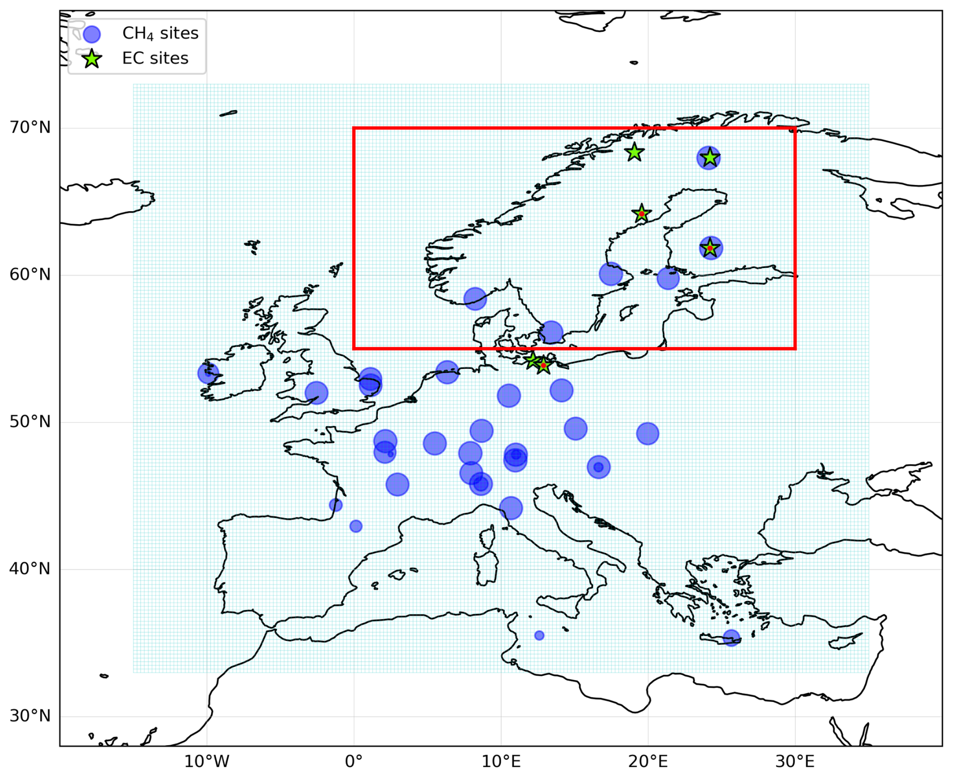
Figure 1 LUMIA inversion domain (cyan grid), the position of the observations used in the LUMIA inversions (blue dots, with the area proportional to the number of assimilated observations); position of the eddy-covariance sites used in the GRaB-AM optimization (green stars) and Nordic domain of interest (red box). The EC sites covering the year 2018 (Fig. 9) are marked with a red dot.

2.1 Wetland emissions modelling

2.1.1 LPJ-GUESS

LPJ-GUESS is a dynamic global vegetation model (DGVM), designed to simulate the interactions between vegetation, soil, and their responses to environmental changes and management (Sitch et al., 2003; Smith et al., 2001, 2014). The model can simulate vegetation dynamics, carbon and water cycles, and soil biogeochemistry from local to global scales, including the simulation of methane fluxes from natural wetlands.

For this study, we used the Arctic-enabled version 4.1 of the model (Smith et al., 2014), which differs from previous versions for having detailed representation of wetland CH₄ emission. The process descriptions of the CH₄ module were mostly adopted from the LPJ-WHyMe model (Wania et al., 2010), and are described in detail in (McGuire et al., 2012). It is based on a “potential carbon pool”, which is then decomposed to soil organic carbon distributed vertically in the soil layers. Methanogens use this decomposed organic carbon and produce CH₄. A part of this produced CH₄ gets oxidized by O₂ and the remainder is transported to the atmosphere by diffusion, ebullition, or plant-mediated transport (see Wania et al., 2010; Kallingal et al., 2024a for more details). The model is driven by daily climate data including air temperature, precipitation, and shortwave radiation taken from the Climatic Research Unit-Japanese Reanalysis (CRU-JRA; Harris et al. (2020) dataset. Annual atmospheric CO₂ concentrations, as additional model input for LPJ-GUESS, are obtained from the Global Monitoring Laboratory (https://gml.noaa.gov/ccgg/trends, last access: 23 October 2025), and the soil property data was extracted from WISE5min, V1.2 Soil Property Database (Batjes, 2005).

Model simulations covering the area north of 45° N are produced using PEATMAP (Xu et al., 2018), which combines geospatial information from various sources to create a global map of wetland extent. PEATMAP has been used in several studies mainly because it is an updated quantification of peat land extend, and it focuses on mapping peatlands, such as marshes and swamps, which are the dominant wetlands in northern latitudes (Peltola et al., 2019; Aalto et al., 2025; Müller and Joos, 2020).

2.1.2 GRaB-AM flux data assimilation framework

To optimize the methane module of LPJ-GUESS, Kallingal et al. (2024a) developed the GRaB-AM data assimilation framework, which seeks to optimize the value of ten highly sensitive parameters in the methane module of LPJ-GUESS (connected to production, transport and consumption pathways of CH₄), based on the model fit to eddy-covariance (EC) flux observations. The minimization is performed using an adaptive scheme of the Markov Chain Monte Carlo Metropolis-Hastings algorithm (Metropolis et al., 1953; Hastings, 1970). In Kallingal et al. (2024b), observations from 14 natural wetlands distributed across the Northern Hemisphere above 40° and over a total period of 20 years (from 2000 to 2020 with individual sites contributing observations over different years within this time period) were assimilated. The number of sites used for the GRaB-AM optimization exceeds the indicated sites shown in Fig. 1 (a full list of the sites is given in Kallingal et al., 2024b).

In this study we computed two ensembles of hundred gridded LPJ-GUESS simulations each, randomizing the values of the LPJ-GUESS parameters adjusted by the GRaB-AM algorithm. In the first ensemble (LPJ-GUESS-unopt) the parameter values were draw from a log transform distribution, such that 90 % of the prior samples fall within their assumed ±40 % uncertainty range. In the second ensemble (LPJ-GUESS-opt), the ensemble members were drawn from the corresponding 90 % confidence interval, to maintain consistency.

2.2 Atmospheric inverse modelling

The consistency of CH₄ emission from LPJ-GUESS (LPJ-GUESS-unopt and LPJ-GUESS-opt) with atmospheric CH₄ mixing ratio measurements was tested using the LUMIA inversion framework. The comparison requires using an atmospheric transport model, and accounting for contributions of other methane sources, and from lateral boundary conditions. The model data mismatches then serve to infer a further correction to the emission estimates.

2.2.1 Inversion approach

LUMIA (Monteil and Scholze, 2021) is a regional atmospheric inversion setup developed initially to estimate European CO₂ inversions using in-situ concentration measurements such as those provided by the ICOS network (Monteil et al., 2020; Munassar et al., 2023; Gómez-Ortiz et al., 2025). This study is the first application to a non-CO₂ tracer.

The inversion seeks to determine the set of regional CH₄ emissions that is the most consistent with a dataset of observed in-situ CH₄ mixing ratios. The impact of emissions outside the regional domain is provided through a prescribed background term. The link between emissions and volume mixing ratio given by:

$$\begin{array}{}\text{(1)}& \mathit{y}+{\mathit{\epsilon }}_o=\mathbf{H}\mathit{x}+{\mathit{y}}_{\mathrm{bg}}+{\mathit{\epsilon }}_{\mathrm{m}}\end{array}$$

with y the observations vector contains observations of the atmospheric CH₄ mixing ratio, and x the control vector contains the variables that we seek to optimise: in our case, the daily CH₄ emissions, grouped in two categories (wetlands and non-wetlands), at a 0.25° resolution over a regional domain ranging from 15° W, 33° N to 35° E, 73° N (Fig. 1). The regional transport operator H contains the sensitivity of the observations y to the (regional) emissions x (${\mathbf{H}}_{i,j}=\partial {\mathit{y}}_i/\partial {\mathit{x}}_j$). The background concentrations (y_bg) are provided as timeseries of baseline concentrations directly at the observation sites, following the two step approach of Rödenbeck et al. (2009) (see Sect. 2.2.3). The error terms ε_o and ε_m represent respectively the measurement error and the model error.

The optimal control vector $\widehat{\mathit{x}}$ is given as the one that minimises a cost function 𝒥(x), such that

$$\begin{array}{}\text{(2)}& \begin{array}{rl}\mathcal{J}\left(\mathit{x}\right)& ={\displaystyle \frac{\mathrm{1}}{\mathrm{2}}}{\left(\mathit{x}-{\mathit{x}}_b\right)}^{\mathrm{T}}{\mathbf{B}}^{-\mathrm{1}}\left(\mathit{x}-{\mathit{x}}_b\right)\\ & +{\displaystyle \frac{\mathrm{1}}{\mathrm{2}}}{\left(\mathbf{H}\mathit{x}+{\mathit{y}}_{\mathrm{bg}}-\mathit{y}\right)}^{\mathrm{T}}{\mathbf{R}}^{-\mathrm{1}}\left(\mathbf{H}\mathit{x}+{\mathit{y}}_{\mathrm{bg}}-\mathit{y}\right)\end{array}\end{array}$$

The first part evaluates the goodness of fit of the estimated control vector x to its prior estimate x_b, normalised by the prior error-covariance matrix B, which contains the uncertainty of x_b. The right hand side term evaluates the model fit to the observations y, normalised by the observation error-covariance matrix R, which combines the model (ε_m) and measurement (ε_o) uncertainties (i.e. it is the total uncertainty on the model-data mismatch).

The optimal control vector $\widehat{\mathit{x}}$, which satisfies ${\mathrm{\nabla }}_x\mathcal{J}\left(\widehat{\mathit{x}}\right)=\mathrm{0}$, is the set of CH₄ emissions that represents the best compromise between fitting the observations and limiting the departures from the prior estimate (which implicitly carries the knowledge of the models and data used to construct the prior emissions).

The solution is searched for iteratively, using a conjugate gradient algorithm provided by the python “scipy.optimize” package (which employs a nonlinear conjugate gradient algorithm by Polak and Ribiere, a variant of the Fletcher-Reeves method described in Nocedeal and Wright (2006). This solver is not optimal for our setup (a linear CG algorithm would be better suited, since our optimization problem is strictly linear), but turned out to be more practical and I/O efficient than the Lanczos (1952) linear solver used in previous LUMIA papers (e.g. Monteil et al., 2020; Munassar et al., 2023), while giving similar results.

2.2.2 Regional transport model

The regional transport operator H was computed using the FLEXPART 10.4 Lagrangian particle dispersion model (Pisso et al., 2019). FLEXPART is not called directly within the inversion, but is used before, to pre-compute observation footprints, i.e. rows of the H matrix from Eq. (2). These footprints are stored on disk and simply read during the successive phases of the inversion. Each footprint was obtained by simulating the dispersion, backward in time starting from the observation time and position, of ten thousand virtual air particles, based on meteorological fields from the ECMWF ERA5 reanalysis (at a 0.25°, hourly resolution), and limited to the aforementioned European domain: the particles are destroyed when they reach the edge of the domain. The aggregated residence time of the particles near the surface (below 100 m above ground) is used as a proxy for the sensitivity of the observations to the emissions.

2.2.3 Boundary conditions

The background vector y_bg accounts for all the contributions to the observed CH₄ mixing ratio that are not adjusted by the inversions: the impact of the initial condition, the impact of CH₄ emissions from outside the regional domain, the impact of European CH₄ emissions having left the domain on the CH₄ mixing ratio of air masses (re-)entering it, and the impact of the various CH₄ sinks (reactions with OH, and, in the stratosphere, with Cl and O(¹D).

The background concentrations were taken from the CAMS v19r1 global CH₄ reanalysis of surface observations (Segers, 2020), which relies on the TM5-4DVAR global atmospheric inversion system. The concentrations baselines were extracted using the two-step scheme of Rödenbeck et al. (2009) (see also Bergamaschi et al. (2022) for the CAMS implementation, and Monteil and Scholze (2021) for the usage in LUMIA). These baselines were provided as part of the CoCO2 CH₄ inversion intercomparison, therefore they are purely an external input to our modeling setup.

2.2.4 Prior emissions and uncertainties

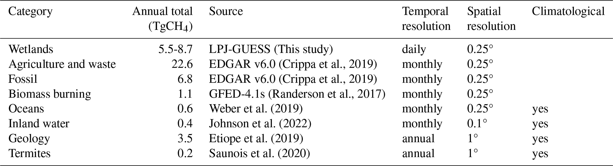
The inversions solve for CH₄ emissions grouped in two “super-categories”: wetland and non-wetlands. The latter groups the contributions of all remaining categories, both anthropogenic (mainly agriculture, waste management and fossil fuel emissions), and natural (geological emissions, termites, lakes and oceans). Anthropogenic emissions are taken from the EDGAR v6.0 emission inventory (Crippa et al., 2019), wetland emissions are taken from the LPJ-GUESS simulations described in Sect. 2.1.1, with or without the parameters optimization described in Sect. 2.1.2 (depending on the simulation). Natural emissions are taken from various climatological estimates, reported in Table 1. All the emissions were regridded from their original resolution to the 0.25°, daily resolution of the FLEXPART footprints.

The spatial distribution of the emissions is shown in Fig. 3, while their temporal distribution is shown in Fig. 2. Wetland emissions are the only category that exhibits a strong seasonality (biomass burning emissions are seasonal as well, but very low overall, so their contribution to the seasonality of total emissions is negligible). There is also a geographical separation between emissions from wetlands, which are concentrated in Northern Europe, and emissions from the other categories, which are more significant in the rest of the continent, and tend to overlap in time and space. This, and the fact that the observation network is relatively dense in Northern Europe (Fig. 1), where wetland emissions are important, justify resolving wetland emissions separately from the other CH₄ sources in the inversions.

The emission uncertainties are stored in the prior error-covariance matrix B, which is composed, for each category c, of four components: the vector ${\mathit{\sigma }}_{x_c}$ containing the standard deviations of the emission themselves, two correlation matrices, $C_c^h$ and $C_c^{\mathrm{t}}$, storing respectively the prescribed correlations in the spatial and in the temporal dimension, and a scalar scaling factor γ_c, which is used to enforce a specified total annual uncertainty. No cross-category correlations are assumed, therefore the error-covariance matrix is written, for each category, as:

$$\begin{array}{}\text{(3)}& {\mathbf{B}}_{\mathbf{c}}=(C_c^{\mathrm{t}}\otimes C_c^h{)}^{\mathrm{T}}{\mathit{\sigma }}_{x_c}^{\mathrm{T}}{\mathit{\gamma }}_c^{\mathrm{2}}{\mathit{\sigma }}_{x_c}(C_c^{\mathrm{t}}\otimes C_c^h)\end{array}$$

For wetland emissions, the standard deviations ${\mathit{\sigma }}_{x_c}$ are set to the standard deviation of the LPJ-GUESS ensembles (Sect. 2.1.1), whereas for non-wetland emissions, they are set to the absolute value of the emissions. The scaling factor γ_c is then determined such that ${\left({\sum }_{ij}{\mathbf{B}}_{\mathbf{c}}^{\mathbf{ij}}\right)}^{-\mathrm{1}/\mathrm{2}}$ equals the desired annual uncertainty for category c. This facilitates comparisons between simulations with different correlation structure, as their overall uncertainty remain identical.

The uncertainties on non-wetland emissions were set to 5 Tg CH₄ yr⁻¹ (≈15 % of the annual emissions), with C^t and C^h constructed as correlation-decay functions ($\mathrm{corr}\left(x\right)=e^{-x/L}$), with horizontal correlation length of 500 km and temporal correlation length of 30 d. For wetlands, the annual uncertainty was set to 0.5 Tg CH₄ yr⁻¹, with temporal correlation length of 30 d. The spatial correlations were either constructed using the same approach, with spatial correlation lengths of 1000 km, in the main inversions (LUMIA-Lprior and LUMIA-Lpost), or directly using the error correlation structure from the LPJ-GUESS ensembles (see Sect. 3.1).

Figure 2 Prior CH₄ emissions used in the “LUMIA-Lprior” inversion.

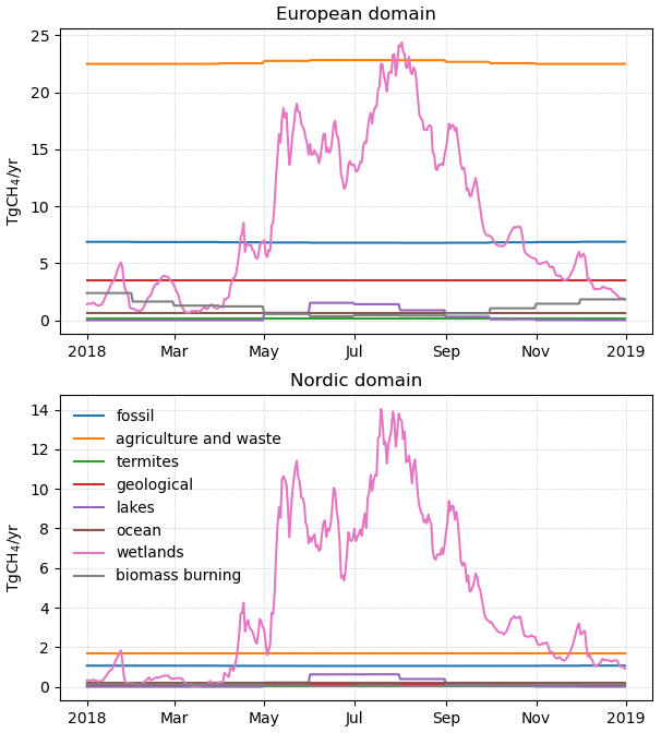
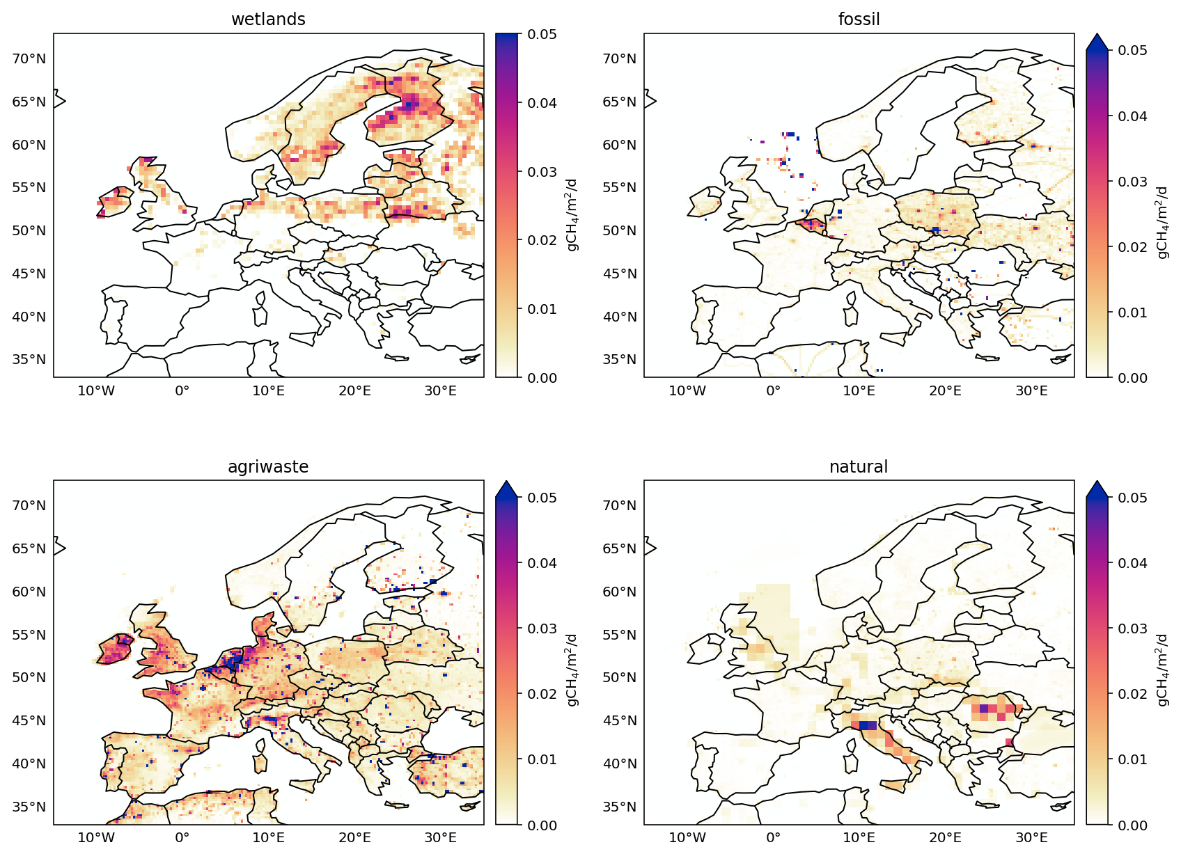
Figure 3 Prior annual average CH₄ emission maps from the natural wetlands, fossil fuels, agriculture and waste and “natural” sectors. The latter groups together emissions from lakes and oceans, geological sources, biomass burning and termites, but is largely dominated by the geological emissions.

(Crippa et al., 2019)(Crippa et al., 2019)(Randerson et al., 2017)Weber et al. (2019)Johnson et al. (2022)Etiope et al. (2019)Saunois et al. (2020)

Table 1 Methane (prior) emissions used in the LUMIA inversions. The spatial resolution reported in the table corresponds to the one as it was made available to us, through the Ioannidis et al. (2025) intercomparison, although the native resolution of some of these products is higher (e.g. EDGAR v6.0 is available at 0.1°).

2.2.5 Observation and observational uncertainties

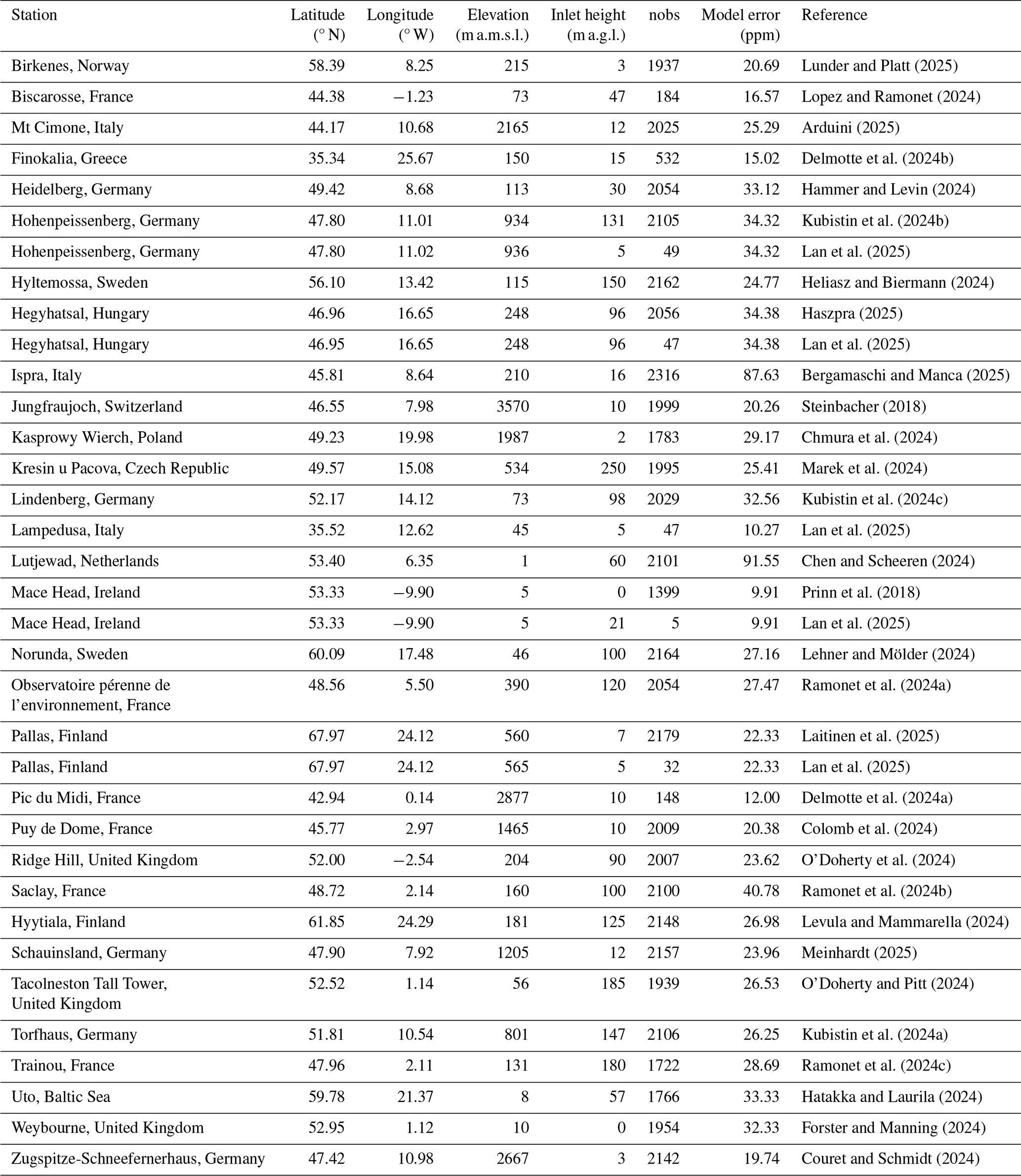
The LUMIA inversions were constrained by observations from 43 European in-situ and flask measurement sites, from various observation networks (see Table 2 and Fig. 1), most of which are now part of the ICOS network of atmospheric in-situ measurements. The observations were taken from a quality controlled dataset prepared for a CH₄ inverse modeling intercomparison conducted within the CoCO2 project (https://coco2-project.eu/, last access: 23 October 2025, Ioannidis et al., 2025).

The observation frequency is typically hourly, but we filtered the observations to avoid assimilating observations close to the transition between the planetary boundary layer (PBL) and the free troposphere, as this is where model errors on the PBL height would have the largest impact. For most sites, afternoon data was selected (from 11:00 to 17:00, local time), when the PBL is expected to be the most developed. For high altitude sites (above 1000 m altitude a.m.s.l), night time data was used instead (from 00:00 to 04:00, local time), when the observations are expected to be well above the PBL. At a few sites (Hohenpeissenberg, Hegyhatsal, Ispra, Mace Hear and Pallas), there are also a some observations from flask measurements, for these, no specific filter was applied.

The uncertainties (diagonal of R in Eq. 2) are set as the quadratic sum of the measurement uncertainty ε_obs, provided by the atmospheric observations dataset, and of the model uncertainty ε_mod. The model uncertainty should in theory be set close to the random component of the error that the model would make when simulating the observations based on the “true” emissions, and excluding systematic component of that error. In practice, that true error is unknown. Here we constructed it as site-specific weekly uncertainty, based on the mismatch between the observed and modelled short term CH₄ variability. The procedure is conducted for each site, in four steps:

1. Compute the prior model estimate for the observations, y_apri, corresponding to the prior emissions described in Sect. 2.2.4.

2. Separate the modelled (y_apri) and observed (y) time series into baselines and anomalies. The baselines are computed as weekly rolling weighted averages (with the inverse of the measurement uncertainties used as weights), and the anomalies are obtained by subtracting these baselines from their respective timeseries.

3. Compute the standard deviation (${\mathit{\sigma }}_{\mathrm{mod}}^{\mathrm{site}}$) of the difference between the anomalies in modelled (prior) and observed CH₄ mixing ratios.

4. The model uncertainty of a single observation is finally given by ${\mathit{\epsilon }}_{\mathrm{mod}}^i={\mathit{\sigma }}_{\mathrm{mod}}^{\mathrm{site}}\times \sqrt{n_{\mathrm{obs}}}$, where n_obs is the number of observations in a ±3.5 d interval surrounding the observation i.

The rationale behind this approach is that the inversions should be able to efficiently reduce the mismatch between the baselines by adjusting the CH₄ emissions, but will likely struggle more with reducing the model-data mismatches between the modelled and observed sub-weekly variability. In practice this results in a larger uncertainty at sites close to large CH₄ emitters, such as Ispra, Saclay and Norunda, reducing their relative weight in the inversion. The last step (4) ensures that the weight of a site doesn't depend on the observation frequency (if there are more observations within a given week, the individual weight of each observation will be reduced accordingly).

Lunder and Platt (2025)Lopez and Ramonet (2024)Arduini (2025)Delmotte et al. (2024b)Hammer and Levin (2024)Kubistin et al. (2024b)Lan et al. (2025)Heliasz and Biermann (2024)Haszpra (2025)Lan et al. (2025)Bergamaschi and Manca (2025)Steinbacher (2018)Chmura et al. (2024)Marek et al. (2024)Kubistin et al. (2024c)Lan et al. (2025)Chen and Scheeren (2024)Prinn et al. (2018)Lan et al. (2025)Lehner and Mölder (2024)Ramonet et al. (2024a)Laitinen et al. (2025)Lan et al. (2025)Delmotte et al. (2024a)Colomb et al. (2024)O'Doherty et al. (2024)Ramonet et al. (2024b)Levula and Mammarella (2024)Meinhardt (2025)O'Doherty and Pitt (2024)Kubistin et al. (2024a)Ramonet et al. (2024c)Hatakka and Laurila (2024)Forster and Manning (2024)Couret and Schmidt (2024)

Table 2 Observation time series assimilated in the LUMIA inversions. The number of observations assimilated is reported in the “nobs” column. Some stations appear twice, when there are both flask and in-situ measurements. The “Model error” column shows the assumed model representation error in the LUMIA-Lprior inversion (${\mathit{\sigma }}_{\mathrm{mod}}^{\mathrm{site}}$). The numbers differ slightly in the LUMIA-Lpost inversion, since they are calculated based on the prior fit to the data. When available, the DOI or PID of the data are shown in their corresponding entry in the bibliography.

3 Results

The LUMIA inversions use wetland emission estimates and uncertainties computed in the two LPJ-GUESS ensembles. We therefore first present the results from these two ensembles, then compare the four CH₄ emission estimates and analyze their consistency with observations.

3.1 Model-derived wetland emission uncertainties

As explained in Sect. 2.2.4, for each category, the prior error-covariance matrix in LUMIA (B in Eq. 2) is constructed based on a combination of prescribed error correlation structure, a vector of (normalized) prior uncertainties and a target annual uncertainty estimate. These settings are typically chosen based on “expert knowledge”. However, for the wetland category, the GRaB-AM setup provides an explicit representation of these error correlations.

The emission uncertainties corresponding to the LPJ-GUESS-unopt and LPJ-GUESS-opt simulations were estimated through two ensemble simulations of 100 members each (see Sect. 2.1.2). The ensemble standard deviation drops from 6.40 Tg CH₄ yr⁻¹ in LPJ-GUESS-unopt to 0.45 Tg CH₄ yr⁻¹ in LPJ-GUESS-opt. In the LPJ-GUESS-unopt ensemble, the uncertainties are concentrated in regions with strong CH₄ emissions: Northern Finland, Scandinavian Arctic, Southern Sweden, Southern Poland and North-West coasts of Ireland and Scotland (Fig. 4). The GRaB-AM optimization reduces the uncertainties everywhere, but predominantly at high-latitudes, with the strongest reduction ($\approx -\mathrm{95}$ %) being obtained in the Nordic region.

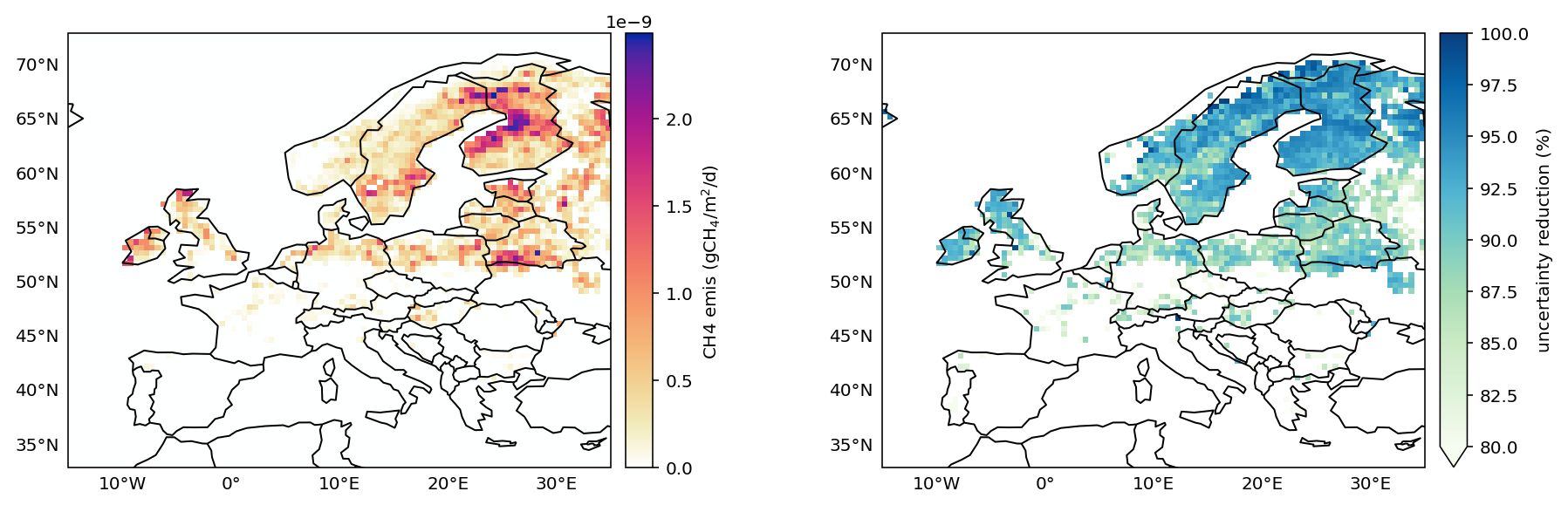
Figure 4 Wetland emission uncertainties, as per the LPJ-GUESS-unopt ensemble (left) and percentage uncertainty reduction in the LPJ-GUESS-opt ensemble (right).

The error correlations are arguably more important for the LUMIA inversions: large error correlations effectively reduce the dimensionality of the problem, making it in turn easier to resolve the contributions from separate categories. Full error covariance matrices can be computed from the ensemble but are too large to fit in memory and be of practical use in the inversions. Instead, in Fig. 5, we show the average error correlations as function of distance (in space and time).

The error correlations are generally larger in the prior ensemble (LPJ-GUESS-unopt) than in the posterior one. In the spatial dimension, there is a lot of variability, but overall, there is a very rapid drop in correlation values, which stabilize around 0.55 in LPJ-GUESS-unopt and around 0.35 in LPJ-GUESS-opt, after approximatively 250 km. The correlations decline further with increased distance, but at a very slow pace. Temporally, correlations decrease almost instantly in LPJ-GUESS-unopt, but remain in a 0.55–0.65 range after that, whereas they decrease more gradually in LPJ-GUESS-opt, reaching below 0.4 after 200 d.

The interpretation of spatial correlations is further complexified by the fact that the number of active CH₄ emission grid cells is not constant throughout the year, and therefore the correlation-distance relationship is not constant. For computing Fig. 5, we ignored the time dimension for the spatial correlations plot, and the space dimension for the temporal correlation plot (therefore, the averaged correlation for two points distant by e.g. 500 km includes the correlation between emission components at different times of the year). This somewhat mimics the way the prior error-covariance matrix B is constructed in LUMIA (i.e. with correlations based on as a Kronecker product of spatial and temporal correlation matrices).

We performed an sensitivity tests to determine the most appropriate formulation for the error-covariances in LUMIA. The two main inversions, LUMIA-Lprior and LUMIA-Lpost, use the wetland error distributions (σ_x in Eq. (3), but correlation matrices based on more traditional exponential correlation-decay functions ($\mathrm{corr}\left(x\right)=e^{-x/L}$), with correlation lengths L_h of 1000 km in C_h (shown in Fig. 5), and L_t = 30 d in C_t, and their domain-wise annual uncertainty was set to 0.5 Tg CH₄ yr⁻¹. This is lower than the variability of the LPJ-GUESS-unopt ensemble, but that variability of that is purposefully unrealistically high to allow GRaB-AM to explore the space of solutions.

In addition, two sensitivity inversions were computed, LUMIA-Lprior+corr and LUMIA-Lpost+corr, which take their annual uncertainty (γ_wetland) directly from the standard deviation of the annual emissions in their corresponding LPJ-GUESS ensemble, and use the ensemble-based correlation-distance relationships shown in Fig. 5. The results were very similar in the Nordic region of interest, therefore for most of the analysis, we choose to rely on LUMIA-Lprior and LUMIA-Lpost. This also acknowledges the fact that ensemble-derived uncertainty estimates ignore errors from the driving data of LPJ-GUESS, and from the processes incorrectly modelled in it. Also, the spatial correlations in the ensembles are not constant through time, therefore the decomposition in a spatial and a temporal correlation matrices is not a very accurate approximation of the actual correlations of the ensemble. Finally, setting the annual uncertainty to the same value in both inversion facilitates the interpretation of the results.

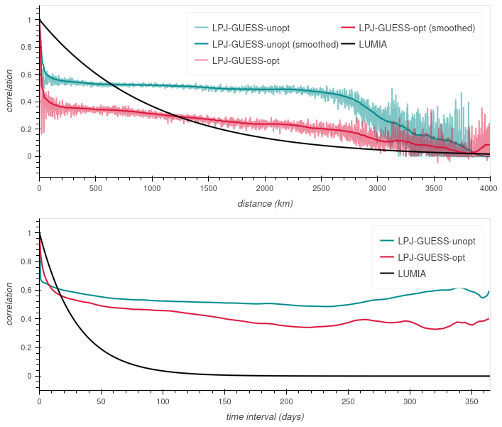
Figure 5 Spatial (top) and temporal (bottom) correlation-distance relationships for the two LPJ-GUESS ensembles. The black line represents the correlation settings used in the LUMIA simulations.

3.2 CH₄ emissions

3.2.1 Annual CH₄ emissions

The non-optimized LPJ-GUESS model (LPJ-GUESS-unopt) points to an emission total of 8.7 Tg CH₄ yr⁻¹ from natural wetlands, including 4.3 Tg CH₄ yr⁻¹ in the Nordic sub-domain. All three observation-informed estimates point to emission reductions ranging from −37 % (LPJ-GUESS-opt, 5.5 Tg CH₄ yr⁻¹) to −51 % (LUMIA-Lpost, 4.3 Tg CH₄ yr⁻¹) at the European scale, and from −42 % (LPJ-GUESS-opt, 2.5 Tg CH₄ yr⁻¹) to −60 % (LUMIA-Lpost, 1.7 Tg CH₄ yr⁻¹) in the Nordic subdomain (Fig. 6). The two sensitivity inversions also lead to very similar results (See full results in Table S1).

In contrast, the inversions lead to much lower adjustments to non-wetland emissions, both in relative and absolute terms. The priors (i.e. LPJ-GUESS-unopt and LPJ-GUESS-opt in Fig. 6) are 35 Tg CH₄ for the full domain, and 34.3 Tg CH₄ yr⁻¹ (−2.8 %) and 35.2 Tg CH₄ yr⁻¹ (−0.1 %) respectively in LUMIA-Lprior and LUMIA-Lpost. The contribution of the Nordic region to this is very small, with 3.3 Tg CH₄ yr⁻¹ in the prior (comparable in magnitude to the wetland emissions in that region). The inversions reduce these to 2.2 Tg CH₄ yr⁻¹ (−33 %) and 2.5 Tg CH₄ yr⁻¹ (−25 %), respectively in LUMIA-Lprior and LUMIA-Lpost. Here again, the difference between the reference inversions and their sensitivity run counterparts is very small.

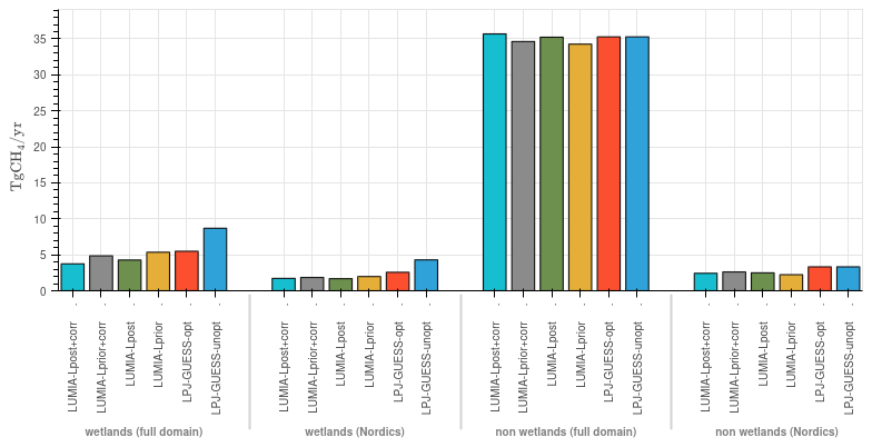
Figure 6 Annual emission estimates (in Tg CH₄ yr⁻¹) for the wetland and non-wetland emission categories. LPJ-GUESS-unopt and LPJ-GUESS-opt are respectively the priors of LUMIA-Lprior(+corr) and LUMIA-Lpost(+corr).

3.2.2 Seasonal cycle of the wetland emissions

Temporal emission adjustments are shown in Fig. 7 (note the different y-ranges in the figure). For the figure clarity, results from the LUMIA-Lprior+corr and LUMIA-Lpost+corr inversions are shown in Fig. S1.

For wetlands, the patterns are very similar between the full-domain and the Nordic region (which reflects the fact that this region accounts for more than half of the European wetland emissions). In LPJ-GUESS-unopt, the emissions remain close to zero in the first quarter of the year, except for two small peaks at the end of January and of March. The emissions then follow a “double-peak” pattern, with a first peak around late May, particularly pronounced in the Nordics, and the main peak in August, after which the emissions decline steadily to reach nearly zero at the end of the year.

The assimilation of in-situ flux data in LPJ-GUESS-opt leads to roughly a halving of the emissions, mainly during the May to October period. Within the Nordic region, the emission peak in May is almost fully preserved, whereas the remaining part of the summer variability is smoothed. Outside the Nordics, the temporal structure of the emissions is better preserved. LPJ-GUESS-opt points to a reduction of the amplitude of the emission peaks in January-February (mostly visible outside the Nordics). On the other hand, the emissions after October remain similar to LPJ-GUESS-unopt.

The two LUMIA inversions lead to emission reduction in the Nordic region that are overall consistent with those obtained in LPJ-GUESS-opt, in particular during the summer months (June-August). Both inversions further attenuate the May emission peak compared to both LPJ-GUESS estimates, and also point to lower emissions than the LPJ-GUESS simulations after August. LUMIA-Lprior essentially retains the seasonal cycle shape of its prior (LPJ-GUESS-unopt), but with a reduced amplitude, whereas LUMIA-Lpost infers corrections to its prior (LPJ-GUESS-opt) only during some parts of the year (May and August–November).

Outside the Nordics (lower left plot in Fig. 7), LUMIA-Lprior also leads to a rather annually uniform scaling down of the wetland emissions, compared to its prior (LPJ-GUESS-unopt). LUMIA-Lpost infers almost no adjustment to its prior (LPJ-GUESS-opt) during most of the year, except during the last months (October to December), when it leads to a signfificant (a third to a half) reduction of the baseline emissions, and also completely erases small emission peaks that LPJ-GUESS simulated at the end of October and beginning of December.

The two sensitivity inversions LUMIA-Lprior+corr and LUMIA-Lpost+corr lead to comparable results, on multi-day averages. However, LUMIA-Lprior+corr displays an extremely high short-term variability (much more that LPJ-GUESS-unopt, its prior). We hypothesize that this is due to the very high uncertainty on wetland emissions used in that simulation (6.4 Tg CH₄, i.e. ≈13 times more than in the other inversions), which, associated to the fact that LPJ-GUESS-unopt tends to alternate (at the grid cell level) between days with strong emissions and days with near zero emissions, makes that inversion very under-constrained. However, on a multi-day average, it is remarkably similar to LPJ-GUESS-opt within the Nordic region, until August, and to LUMIA-Lprior for the rest of the year, and also in the rest of Europe.

Compared to LUMIA-Lprior, LUMIA-Lprior+corr follows very closely the seasonal variability of their prior (LPJ-GUESS-opt), shifting it only by a seemingly constant scaling factor. This is a consequence of the very long distance correlations from the LPJ-GUESS ensemble (see Fig. 5), which reduces drastically the degrees of freedom of the inversion, even though the observations provide sufficient constraint to resolve finer scale patterns.

3.2.3 Temporal variability of the other emissions

The temporal adjustments of the “non-wetland” emission category groups contributions from many source processes, mainly anthropogenic, which makes them difficult to interpret at the domain-scale. In the Nordics, the LUMIA inversions infer, on average, a reduction of the non-wetland emission of 25 % (LUMIA-Lpost) to 32 % (LUMIA-Lprior), with large variations throughout the year, with a peak increase of up to 35 % (LUMIA-Lpost, in August), and a reduction to near zero towards the end of the year.

A part of this variability is likely caused by misattributions of emission corrections between the two emission categories. For instance, from April to July, the non-wetland emissions of LUMIA-Lprior in the Nordics are significantly lower than those inferred in LUMIA-Lpost, which compensates for an opposite sign difference between these two inversions in the wetland emission category. However, while the reduction in non-wetland emissions towards the end of the year doesn't appear probable given the expected stability of anthropogenic emissions over the year, re-allocating it entirely to the wetland emission category would lead to (significantly) negative wetland emissions, which isn't realistic either.

A possible alternative (or complementary) explanation could be error in the CAMS boundary condition: the background concentrations (y_bg in Eq. 2) explains nearly 100 % of the observed mixing ratio on several days towards the end of the year, especially at Hyytiälä (SMR) and Birkenes (BIR). The situation is also similar in the two sensitivity inversions.

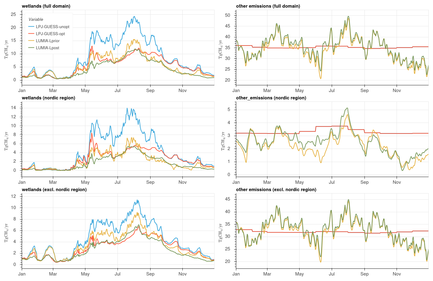
Figure 7 Daily emissions in the entire domain (top), in the Nordic region (middle) and outside it (bottom), for the wetland (left) and non-wetland (right) CH₄ emissions.

3.2.4 Spatial distribution

The emission adjustments inferred in GRaB-AM and LUMIA optimizations are shown in Fig. 8. To facilitate the comparison, wetland adjustments in LUMIA-Lpost are shown relative to the unoptimized LPJ-GUESS estimate (LPJ-GUESS-unopt). Maps for the sensitivity inversions are can be found in Figs. S2, and S3 shows the maps relative to LPJ-GUESS-opt.

The spatial distribution of wetland emission adjustments is very similar in the five data-informed products, and largely proportional to the LPJ-GUESS-unopt emission estimate itself. The long error-correlations imposed on the LUMIA inversions (and intrinsic to the GRaB-AM optimization), combined with the relative concentration of wetland emissions in Northern Europe, ensure a convergence between the localization of flux corrections.

Among the most marked features in the adjustment to the “non-wetland” category, we note a doubling of the emissions in the Bretagne region of France, and in the Northern part of the Netherlands. This could point to underestimated agricultural emissions, which are important in these two regions. Another marked feature is an important (≈80 %) reduction of the emissions in Northern Italy, which is well correlated with both high natural emissions (mainly geological) and high agricultural emissions.

We, however, need to ascertain a level of care when interpreting these emission adjustments: For instance emissions in the west of the continent can also result from the need to correct an inaccurate boundary condition. There can also be compensating effects between adjustments of emission hotspots, such as the city of Paris or the Po Valley, and their surroundings. These emission corrections should be investigated, but fall outside the scope of our study.

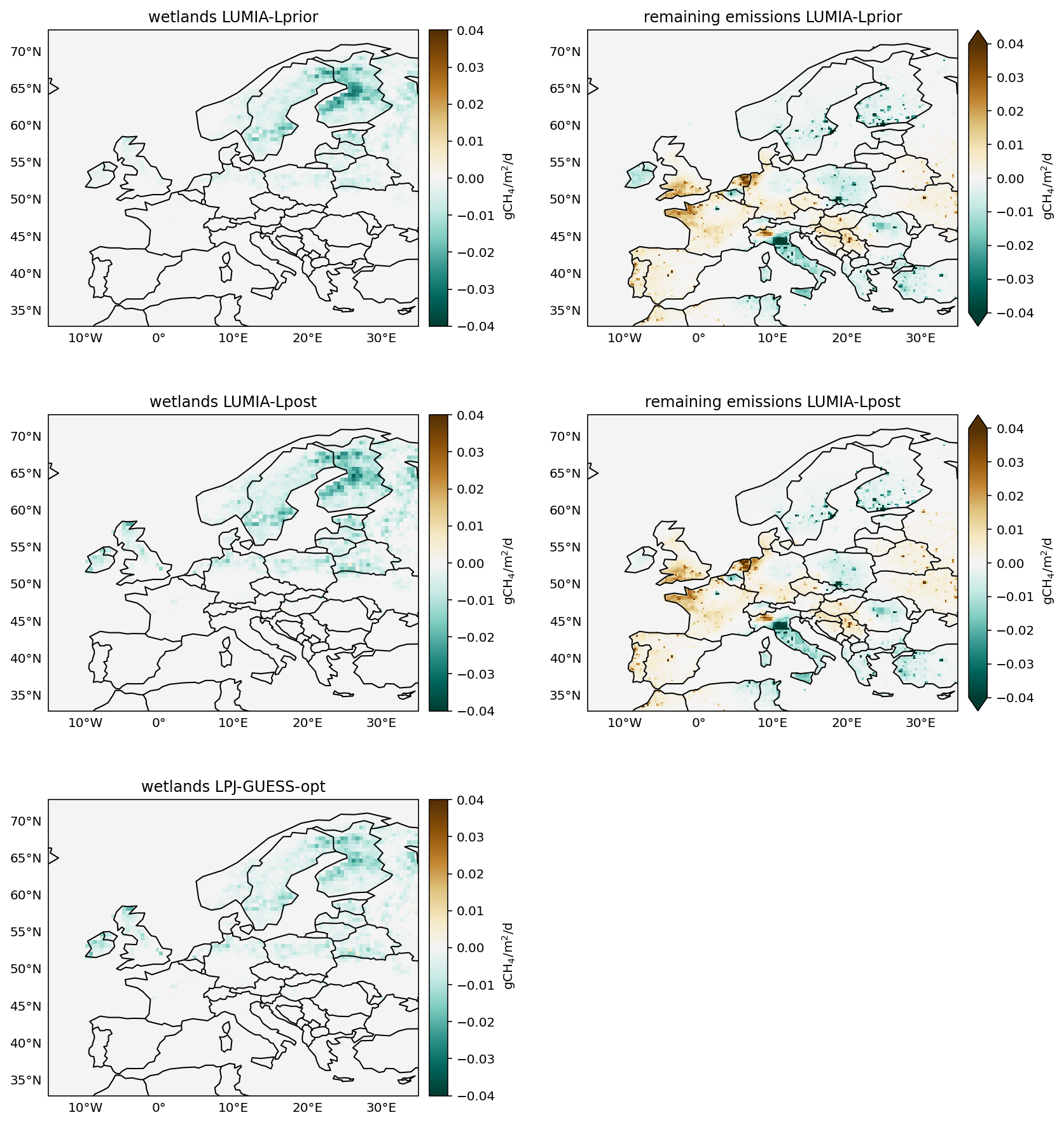
Figure 8 Emission adjustments for wetlands (left) and non-wetlands (right) in the three data-informed simulations, compared to the unoptimized LPJ-GUESS model (LPJ-GUESS-unopt).

3.3 Fit to observed data

A classical diagnostic in data assimilation is to compare results (optimized emissions or concentrations) to independent measurements. For GRaB-AM, such a validation has been conducted in Kallingal et al. (2024b). For atmospheric inversions, the comparison is generally made with independent observations of the atmospheric composition, keeping in mind that biases due to the transport model would likely affect similarly the fit to assimilated data and to validation data.

For this study however, most of the available data in the Nordics has been assimilated, either in the LUMIA inversions (for concentration data), or in the GRaB-AM assimilation (for in-situ flux measurements). The aim of the model-data comparisons in this section is therefore not to derive an objective metric of the respective qualities of each emission estimates, but rather to gain insights on the forcings that lead to these emission adjustments.

3.3.1 Eddy-covariance flux estimations

CH₄ emissions can be estimated locally on wetland scales using flux measurement techniques such as Eddy-covariance measurements, which involve capturing the covariance between the vertical wind speed and the concentration of methane, providing high-resolution data on gas exchange over wetlands. Such observations are for instance provided by the ICOS network in Europe (ICOS RI et al., 2024), and the FLUXNET-CH₄ dataset globally (Pastorello et al., 2020; Delwiche et al., 2021), which offers aggregates of high-quality CH₄ flux measurements from wetlands. These networks try to offer a comprehensive coverage of the different types of wetlands (with differences in physiological features such as hydrology, soil characteristics, vegetation types, etc., and in spatial features, such as geographical distribution, size, landscape position and topography).

However, a direct comparison with gridded emissions is difficult, as the latter accounts for average conditions over the grid cells, which can be very different from the local ones. This is illustrated in Fig. 9, which shows a comparison between our four main emission estimates and in-situ flux measurements at three sites in the Nordic region (Zarnekow is slightly outside the Nordic domain used for the emission comparisons, see Fig. 1), along with the site-level LPJ-GUESS simulations which were used to train the GRaB-AM optimization (see Sect. 2.1.2).

The fit of the modelled emissions against the observations is improved for most sites (clearly shown for e.g. Siikaneva and Degero) but since the GRaB-AM optimization is seeking for an optimal parameter set fitting multiple sites simultaneously it is not surprising that there are still larger differences between simulated emissions and observations for any given individual site (as is the case for Zarnekov where the calibrated LPJ-GUESS model fails to simulate the observed peak values during August 2018).

The site-level simulations achieve systematically a better fit to the observations than their corresponding gridded products. Among the gridded products, the best fit is obtained by LUMIA-Lpost, at Siikaneva and Degero, with RMSE reduction above 61 % (Table 3), whereas the error reduction is lower at Zarnekow, with all the data-informed product in a 17 % to 21 % RMSE reduction range. The two sensitivity inversions using ensemble-derived covariances lead to slightly worse fit than the base LUMIA inversions. We also note a tendency of the LUMIA inversions using LPJ-GUESS-unopt as a prior to infer significant negative emissions on some days (Fig. S4): LUMIA adjusts the emissions but preserves most of their original day-to-day variability, which results in days with negative emissions.

Table 3 Mean bias and percentage RMSE reduction, compared to the LPJ-GUESS-unopt site simulation (i.e. negative RMSE reduction values indicate a larger RMSE than the LPJ-GUESS-unopt site simulation), at the three eddy-covariance sites represented in Fig. 9.

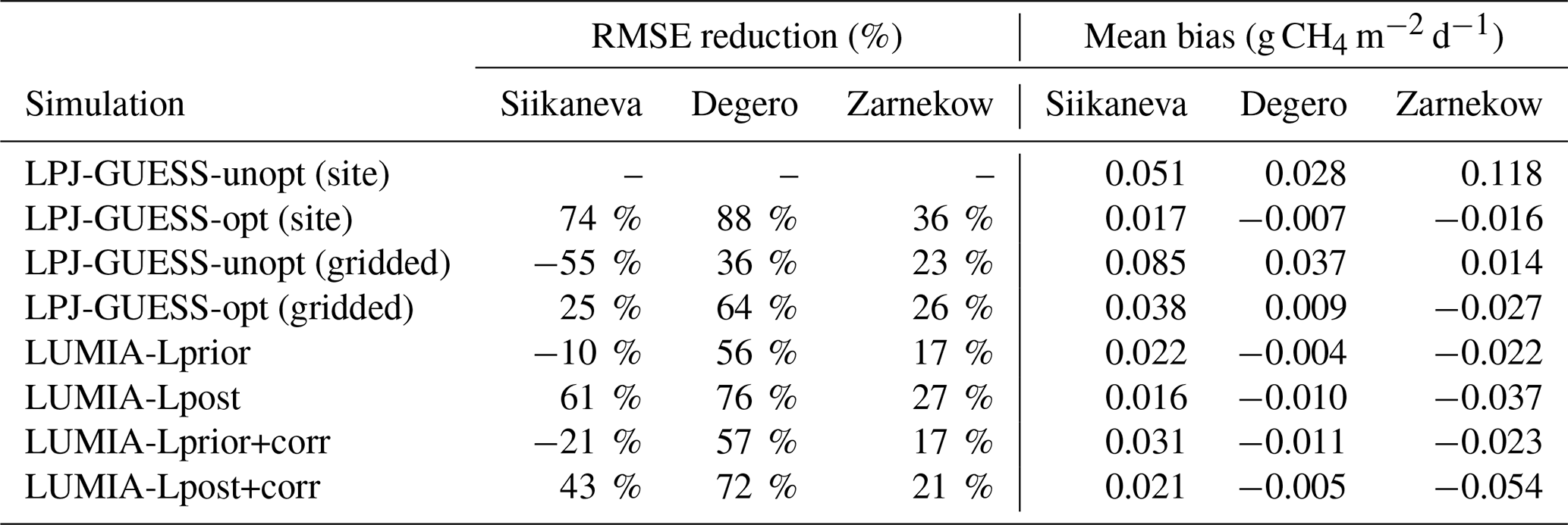
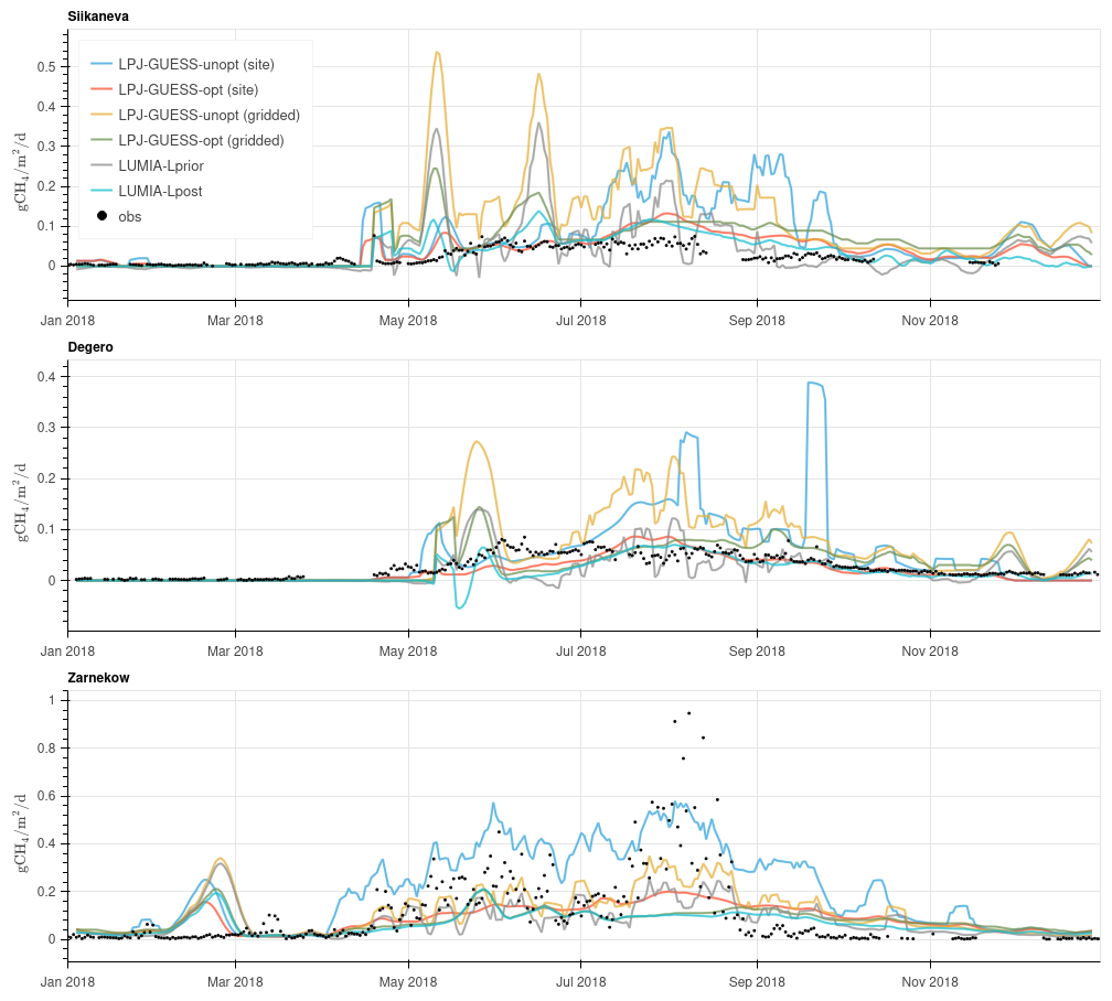
Figure 9 Modelled (solid lines) and observed (dots) methane emissions at three sites within the Nordic region. All the values are expressed in CH₄ emissions per square-meter of wetland. For clarity of the figure, a weekly rolling average has been applied to the modelled data. A version of this figure without smoothing can be found in supplementary materials.

3.3.2 Atmospheric CH₄ observations

The CH₄ concentrations corresponding to the four methane emission estimates are shown in Fig. 10, for the six sites in the Nordic region. These sites are also among the ones where the relative contribution of wetland emissions to the foreground concentrations (i.e. the part of the concentrations that can be adjusted by LUMIA) is the highest. For figure clarity, a two-days rolling average has been applied to the the modelled timeseries, while the data without weekly averaging is shown in Fig. S5.

LPJ-GUESS-unopt leads to an overestimation of the concentrations throughout the summer (with a mean bias of up to 18 ppb at Norunda, and peak model-data mismatches exceeding 200 ppb). The fit obtained using LPJ-GUESS-opt emissions is more in line with the observations, with mean biases ranging from −2.1 ppb at Hyltemossa to +14.1 ppb at Hyytiälla. However, the CH₄ concentrations are still significantly overestimated towards the end of the year at Pallas, Norunda and Hytiälla.

Both LUMIA inversions lead to very comparable results in terms of mean bias, with a tendency to underestimate the observations (with biases ranging from −0.5 ppb at Utö, down to −5.4 ppb at Hyltemossa). However, they lead to a significant RMSE reduction compared to the LPJ-GUESS simulations, with RMSE values in a 12.8 to 17 ppb range (slightly lower in LUMIA-Lpost).

The slightly worse statistics of the LUMIA inversions in terms of bias compared to LPJ-GUESS-opt at the Hyltemossa site (and to a lesser degree also at Birkenes) is likely due to a misfit of observations during the first two weeks of the year, when there is very little flux adjustments that the inversions can infer since the prior emissions start on 1st January. However, the bias is well below the typical prescribed model-data mismatches (which are on the order of 30 ppb), and the RMSEs are reduced as expected. Nonetheless, this points to a possible slight underestimation of the emissions by the inversions.

On the other hand, the overestimation of the observations in the LPJ-GUESS-unopt simulation is very large and a clear indication that the emissions modelled by the non-optimized LPJ-GUESS in the summer are refuted by the atmospheric observations (and to a lesser extent, for the optimized LPJ-GUESS simulation). Other sources of uncertainties (transport model error, uncertainty on the background concentrations, uncertainty in non-wetland emissions) don't seem large enough to account for such an overestimation of the observed data.

Table 4 Fit statistics (bias and RMSE, in ppb) of the LUMIA simulations, for the six sites shown in Fig. 10.

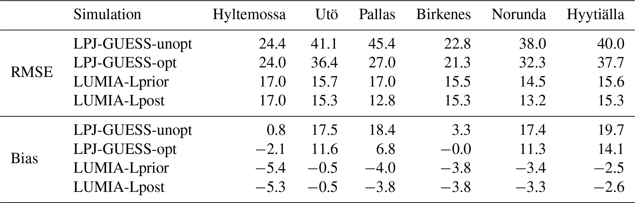
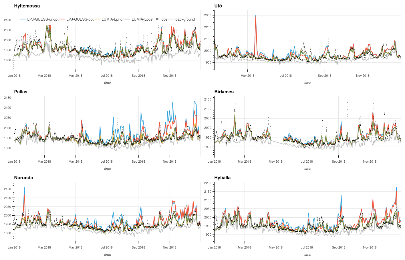
Figure 10 Modelled (solid lines) and observed (dots) CH₄ mixing ratio at the six observation sites within the Nordic region. Modelled time series are shown with as two-days rolling average. A non-smoothed version of the figure can be found in Fig. S5.

4 Discussion

Our study combines two data-informed, in principle complementary, data assimilation approaches: the parameter estimation approach (GRaB-AM) is process-specific and can lead to improvements in the prognostic capabilities of the underlying process model (LPJ-GUESS), but remains subject to possible large scale biases, both because of the lack of representativity of the assimilated data and the inaccuracy of LPJ-GUESS. The inverse approach, LUMIA, is arguably more reliable at large scales, but lacks spatial and process resolution.

In this context, the development of a full CH₄ emission data assimilation system (CH4-DAS), combining a vegetation and an atmospheric transport model and capable of assimilating both eddy-covariance measurements and atmospheric CH₄ observations appears as the next logical step. Such systems have been developed successfully for CO₂ (Rayner et al., 2005) and have shown promising results. For methane however, the development is complicated by the need to account for non-wetland methane emissions, which although less uncertain in relative terms, dominate the emission and emission uncertainty budget in absolute terms (Saunois et al., 2020), and by the complexity of wetland models, which can be highly non linear (Kallingal et al., 2024b).

As an intermediate solution, our study explores a two-step approach, with an atmospheric inversion informed by emission estimates and error correlations from a CH₄ parameter estimation approach. In the following sections we further discuss the potential and limitations of both approaches, and how they can help us improve the LPJ-GUESS model.

4.1 LPJ-GUESS parameter estimation (GRaB-AM)

The GRaB-AM approach aims at optimizing specifically wetland emissions, by fitting a DGVM (LPJ-GUESS) to eddy-covariance (EC) measurements. The resulting emission estimates inherits the spatio-temporal structure from the process parametrizations implemented in the model. This ensures that the emissions remain consistent with their assumed relationships to factors such as climate and environmental forcings. Overall, it should improve the predictive capacity of the model but can also lead to large systematic errors if the aforementioned parametrizations are insufficiently accurate, if the sites used for training are not representative enough, and/or if the selection of parameters to resolve doesn't provide the necessary degrees of freedom to fit the data. A specific difficulty encountered in GRaB-AM is the high non-linearity of LPJ-GUESS which makes it very challenging to design a minimization algorithm that avoids getting local minima and/or parameter equifinality issues.

The LPJ-GUESS-opt methane emissions used in this study were taken from a multi-site application of the GRaB-AM parameter estimation (Kallingal et al., 2024b). The comparison to atmospheric CH₄ observations and to LUMIA inversion results confirm that, overall, GRaB-AM does lead to an improvement in the quality of the LPJ-GUESS CH₄ emission estimate, with annual emission estimates comparable to those obtained through the atmospheric inversions. While this provides a form of validation for GRaB-AM, the comparisons to atmospheric data still shows a tendency to overestimate CH₄ concentrations, in particular in winter (Fig. 10). This is also to some extent the case in comparisons with eddy-covariance measurements. This could point to necessary improvements in the underlying LPJ-GUESS model; Kallingal et al. (2024b) mentioned in particular the simplistic representation of ebullition and the assumption of zero wind speed above wetlands. Uncertainties in the prescribed wetland area extent could also play a role: the spatial extent of wetlands can vary interannually, depending on hydrological factors such as precipitation, evapotranspiration, and water table depth. However, PEATMAP Xu et al. (2018), which is used in LPJ-GUESS, doesn't capture this variability. Xu et al. (2018) highlights this as a key limitation, noting that the use of static distributions can introduce significant uncertainty, especially in regions with strong seasonal or interannual variability in inundation. Finally, the GRaB-AM optimization did not include a parameter that directly controls the sensitivity of the CH₄ emissions to temperature, following an initial parameter sensitivity analysis conducted on a single-site experiment in Kallingal et al. (2024a). However, our results could indicate an exagerated sensitivity to temperature, as indicated by the persistent emission peak in May, in both the LPJ-GUESS -opt and -unopt ensembles. In this case it would be beneficial to integrate the temperature dependency to the parameter estimation if future applications of GRaB-AM.

4.2 Atmospheric inversion (LUMIA)

This study is the first application of LUMIA inversions to a non-CO₂ tracer. Compared to the latest CO₂ applications (Munassar et al., 2023; Gómez-Ortiz et al., 2025), the inversion setup has been simplified: the inversions adjust the emissions directly, instead of offsets to the prior emissions in these studies. This is permitted by the comparatively lower temporal variability of the methane emissions. The uncertainties are of two orders: First, inversions rely on a transport model to establish the link between observed CH₄ mixing ratio and emissions, which can bring systematic errors. Secondly, the source attribution of the emission adjustments depends for a large part of the prescribed emission uncertainties and error correlations.

The original aim was to construct the wetland emission error-covariance matrices based on the variability of the LPJ-GUESS ensembles of CH₄ emissions. These ensembles contain long distance correlations (see Fig. 5), which would theoretically provide constraints to help resolve the relative contribution of wetlands to the total CH₄ emissions. However, this carries the risk of producing biased results if these correlations are not accurate, which is likely, given the limitations highlighted in the previous section. We therefore opted for a more conventional approach to constructing the error-covariance matrices in LUMIA-Lpri and LUMIA-Lpost, using the ensemble variability only to distribute a prescribed annual uncertainties in time and space. Results within the Nordic region of interest were very similar to those obtained in the “+corr” sensitivity runs, which is an indication that, in this region, the observations provide robust enough constraints on the emissions.

The uncertainty associated to transport is difficult to assess independently. Comparisons to independent (i.e. non assimilated) observations rely on the same model to estimate the link between concentrations and emissions, therefore they don't constitute a totally independent validation of the source-concentration relationships themselves. Model intercomparisons, such as TRANSCOM for global models (Gurney et al., 2004), and EUROCOM for regional models (Monteil et al., 2020) can help identifying divergences between models and inversion approaches. A detailed intercomparison was conducted between the LUMIA and CarboScope-Regional (CSR) inversion systems to quantify the importance of model biases in regional CO₂ inversions (Munassar et al., 2023), which highlighted a stronger sensitivity to emissions in LUMIA. While this could lead to overestimating the methane concentrations (given the correct emissions), the amplitude of the mismatches in LPJ-GUESS-unopt, and the fact that they occur specifically in regions with important wetland emissions rather plead for a significant overestimation of the methane emissions by LPJ-GUESS.

Both inversions suggest an almost complete reduction of non-wetland emissions towards the end of the year in the Nordic region, which doesn't seem likely given the importance of fossil-fuel emissions in that non-wetland emission category. Comparisons with eddy-covariance data (Fig. 9) show an overestimation of emissions from wetlands at Siikaneva and Zarnekow during that period, suggesting possible misattribution of the emission corrections to the non-wetland category. On the other hand, fully re-allocating these corrections to wetlands would imply negative emissions, which is also implausible. We noted that the CAMS background concentrations were very close to (or even occasionally higher than) the observed values in winter, especially at Pallas and Hyytiälä (Fig. 10): as widespread negative emissions of CH₄ are unrealistic, this points to an overestimation of the background concentrations by the CAMS concentration baselines, and a possible widespread bias in the inferred emission totals, although it is difficult to determine whether it affects the whole inversion period or just the winter months.

Some inversion systems allow the boundary condition to be adjusted (e.g. Steiner et al., 2024), but this is risky in the absence of a proper quantification boundary condition uncertainty and of its variability. Here, the non-wetland emission category partly acts as a bias correction, but we must acknowledge this issue as a remaining source of uncertainty.

4.3 Refined estimate of European methane emissions at high latitude

We have refined the wetland emission estimate in the Nordic region to a range of 1.7 Tg CH₄ yr⁻¹ (LUMIA-Lpost) to 2.5 Tg CH₄ yr⁻¹ (LPJ-GUESS-opt), significantly down from 4.3 Tg CH₄ yr⁻¹ in the original LPJ-GUESS-unopt estimate. While the difference between the LPJ-GUESS-unopt and the other estimates is large, the relative qualities of the three data-informed products are more difficult to assess.

The inversions lead to an improved representation of atmospheric observations, compared to LPJ-GUESS-opt, and LUMIA-Lpost also yields a slight improvement in the fit to eddy covariance data, compared to the gridded LPJ-GUESS-opt product. The better fit to the eddy-covariance data by the site-specific LPJ-GUESS simulations (Fig. 9) is expected since (1) GRaB-AM has already maximized the fit to these data, leaving only limited scope for improvement to LUMIA, and (2) these simulations use site-specific meteorological forcings, whereas the emissions in LUMIA and in the gridded LPJ-GUESS simulations are representative of larger 0.25°×0.25° grid cells. Nonetheless, the estimates in LUMIA could also be impacted by systematic error, such as biases from the boundary condition, transport model errors (as highlighted in Munassar et al., 2023), or category attribution errors, as discussed in the previous sections.

Direct comparisons with other studies are complicated because of the small size of our Nordic domain, and other vegetation models have their own shortcomings, and are therefore not necessarily more realistic than LPJ-GUESS. Nonetheless, in a comparison of Arctic wetland emission estimates from six different vegetation models, Aalto et al. (2025) found that, although not a complete outlier, LPJ-GUESS to be clearly at the high end of the range. In the Ioannidis et al. (2025) European CH₄ inversion intercomparison, in the framework of which our LUMIA CH₄ setup was developed, the JSBACH-HIMMELI model (Susiluoto et al., 2018; Raivonen et al., 2017; Petrecsu et al., 2023) was used to provide prior wetland emissions. For the same Arctic domain, the annual wetland emissions add up to 1.3 Tg CH₄, 23 % lower than the ones in LUMIA-Lpost (Fig. 11). LUMIA-Lpost is also the closest to JSBACH-HIMMELI in terms of seasonality, with a summer maximum in August, and near zero emissions in winter time.

Taken together, these comparisons would point at LUMIA-Lpost being the most realistic of our three wetland emission estimates. The contribution of wetlands from our Nordic domain to the overall wetland CH₄ emission budget is however very small, but it suggests a benefit of repeating the study, with an improved setup, over a wider pan-Arctic region.

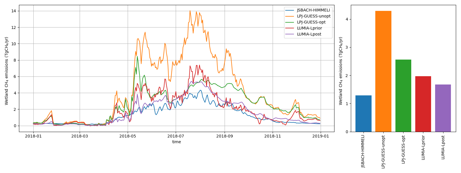
Figure 11 Wetland CH₄ emissions in the LPJ-GUESS and LUMIA products, compared to the JSBACH-HIMMELI emission estimate from Ioannidis et al. (2025).

4.4 Towards a coupled flux-concentration CH₄ data assimilation system

The initial aim of the study was the implementation of a two-step estimation approach, with a transmission of uncertainty between the vegetation model parameter estimation (GRaB-AM) and the atmospheric inversion (LUMIA). Two main complications were encountered: first, the error structure from the parameter estimation step could not be easily approximated in a form usable by the inversion (i.e. as a set of standard deviations and spatial and temporal correlation matrices). This purely technical limitations could be overcome, e.g. by using an ensemble minimization approach in LUMIA, which usually don't need an explicit representation of the error covariance matrices (e.g. Bisht et al., 2023).

A more fundamental issue is the complexity of LPJ-GUESS (and of dynamic global vegetation models in general). The heavy parametrization, non linear interactions, and tightly coupled processes (e.g. photosynthesis, allocation, soil moisture, plant types, etc.) in the model make its calibration against EC data computationally demanding and prone to equifinality. However, increased complexity doesn't necessarily translate in higher predictive performance (Famiglietti et al., 2021). The development of diagnostic models for wetland methane emissions, e.g. McNicol et al. (2023); Bernard et al. (2025), similar to those existing for CO₂ (Mahadevan et al., 2008; Knorr and Heimann, 1995; Potter et al., 1993), could help overcome these limitations. In contrast to DGVMs, diagnostic models do not attempt to simulate ecosystems, but focus solely on empirical parameterizing of their emissions based on a handful of known or observable or externally modelled parameters (e.g. net primary production, water table depth, temperature, etc.). Alternative diagnostic models based on Machine Learning (ML) algorithms remove the need to explicitly formulate relationships between the observables and the inferred CH₄ emissions (e.g. Virkkala et al., 2025; Ying et al., 2025; Ross et al., 2024). This however limits their scope to studying emissions during the observable period (i.e. the past few decades at most), and DGVMs will remain needed for their long-term predictive capabilities, therefore it is crucial to ensure that data assimilation experiments such as ours eventually lead to improvements in the DGVMs.

In the past years, subsequent work has also been conducted by the anthropogenic emission inventory compilers to produce uncertainty estimates (e.g. Solazzo et al., 2021), which should lead to a better representation of the anthropogenic emission uncertainties in inversions, and in turn improve the reliability of their source attribution.

5 Conclusions

We have performed European CH₄ inversions using the LUMIA regional atmospheric inversion system. Prior estimates for methane emissions from wetlands, as well as the associated uncertainties, were taken from a parameter estimation of the LPJ-GUESS model (GRaB-AM, Kallingal et al., 2024b), while prior emissions from other methane sources were taken from conventional emission inventories (e.g. EDGAR 6.0 for anthropogenic emissions). The primary objective was to compare and cross-validate the two optimization approaches, but we also wanted to determine whether the additional constraints from eddy-covariance data could help the inversion resolve not only the total CH₄ emissions, but also the contribution from wetlands to this total.

We focused most of our analysis on emissions from wetlands in the Nordic region (0° E, 55° N; 30° E, 70° N), where wetlands dominate the emission budget: this limits the risk that the inversions incorrectly allocate emission adjustments between the wetland and non-wetland categories. We found a strong agreement between the different data-informed approaches (GRaB-AM, informed by EC data; LUMIA, informed by atmospheric CH₄ measurements; and LUMIA constrained by wetland emissions from GRaB-AM, informed by both observation types): all three approaches point to a strong (by a factor two to three) overestimation of the CH₄ wetland emissions by the un-optimized LPJ-GUESS model. The GRaB-AM approach leads to significant improvement of the fit to atmospheric data (which it didn't assimilate), which constitutes a form of additional validation for the approach. The inversion using prior wetland emissions from GRaB-AM also lead to the best overall fit to observations.

We have explored implementing a more complete uncertainty transmission between the parameter estimation and atmospheric inversion steps, constraining the LUMIA inversions with error correlations from the GRaB-AM LPJ-GUESS ensembles. In theory, the long distance correlations in these ensembles should let us extend our analysis to regions where wetland emissions are significant but contribute a smaller fraction of the emission total. However, despite an improved agreement to atmospheric observations, the fit of LPJ-GUESS to eddy covariance data remains sub-optimal, even after the GRaB-AM parameter estimation, suggesting that these error correlations may not be entirely realistic. This points either to shortcomings in LPJ-GUESS itself, or to the need to include more degrees of freedom in the GRaB-AM approach, by increasing the number of parameters, to allow a more realistic fit to the eddy-covariance data in multi-site experiments.