the Creative Commons Attribution 4.0 License.
the Creative Commons Attribution 4.0 License.
 | 29 Oct 2025
Investigating KDP signatures inside and below the dendritic growth layer with W-band Doppler radar and in situ snowfall camera
Anton Kötsche
Alexander Myagkov
Leonie von Terzi
Maximilian Maahn
Veronika Ettrichrätz
Teresa Vogl
Alexander Ryzhkov
Petar Bukovcic
Davide Ori
Heike Kalesse-Los
Polarimetric radars provide variables like the specific differential phase (KDP) to detect fingerprints of dendritic growth in the dendritic growth layer (DGL) and secondary ice production, both critical for precipitation formation. A key challenge in interpreting radar observations is the lack of in situ validation of particle properties within the radar measurement volume. While high KDP in snow is usually associated with high particle number concentrations, only few studies attributed KDP to certain hydrometeor types and sizes. To address this, we combined surface in situ observations from the Video In Situ Snowfall Sensor (VISSS) with remote sensing data from a polarimetric W-band radar and an X-band radar, along with modeling approaches. Data were collected during the CORSIPP project, part of the ARM SAIL campaign (winter 2022/2023, Colorado Rocky Mountains). We found that at W-band, KDP > 2 ° km−1 can result from a broad range of particle number concentrations, between 1 and 100 L−1. Blowing snow and increased ice collisional fragmentation in a turbulent layer enhanced observed KDP values. T-matrix simulations indicated that high KDP values were primarily produced by particles smaller than 0.8 mm in the DGL and 1.5 mm near the surface. Discrete dipole approximation simulations based on VISSS data suggested that dendritic aggregates larger than 2.5 mm contributed 10 %–20 % to the measured W-band KDP near the surface. These findings highlight the complexity of interpreting W-band KDP in snowfall and emphasize the need for combined in situ observations and radar forward simulations to better understand snowfall microphysical processes.
- Article
(17957 KB) - Full-text XML
- BibTeX
- EndNote


More than 60 % of global precipitation is generated through the ice phase (Heymsfield et al., 2020); therefore, research into the microphysics of the ice and mixed phase has intensified in recent years. The dendritic growth layer (DGL), a temperature region roughly between −10 and −20 °C, plays a major role in the formation of precipitation through the ice phase. In the DGL, the difference between the saturation vapor pressure over ice and water is maximized (Wegener–Bergeron–Findeisen process (Wegener, 1911; Bergeron, 1935)), which leads to a rapid growth of ice into very anisotropic plate-like shapes (Takahashi, 2014) while the number concentration is increased through secondary ice production (SIP) mechanisms (e.g., Von Terzi et al., 2022). A distinct secondary particle mode linked to the formation of new anisotropic particles may be observed at the top of the DGL as a bimodality in Doppler spectra from vertical pointing measurements (e.g., Moisseev et al., 2015). The origin of this secondary mode is still debated, theories about its formation were summarized in Von Terzi et al. (2022). Potential sources include sedimentation of ice particles, primary nucleation due to upward air motion, and some form of SIP mechanism.
SIP has been identified as a key mechanism that enhances ice particle concentrations at temperatures above the homogeneous freezing temperature (Korolev and Leisner, 2020). SIP involves mechanisms that increase the number of ice particles without directly relying on primary ice nucleation through ice nucleating particles (INPs) (e.g., Hoose and Möhler, 2012; Kanji et al., 2017) or homogeneous freezing at very low temperatures (e.g., Sanz et al., 2013). As mountainous regions around the globe act as natural water reservoirs, storing water in the form of snow and ice, a special focus is put on microphysical processes leading to snow formation in mountain regions. Wind shear and associated turbulence were found to impact precipitation production and ice microphysics in multiple studies in recent years (e.g., Grazioli et al., 2015; Ramelli et al., 2021; Dedekind et al., 2023). Grazioli et al. (2015) proposed that splinters from SIP processes can be recirculated in the layer of shear and grow into small oblate ice particles. The area above a shear layer is supplied with supercooled liquid water (SLW) and ice crystals produced inside the turbulent updrafts. This can favor the growth of anisotropic ice crystals in this region and is suspected to cause enhanced ZDR signatures (Hogan et al., 2002; Grazioli et al., 2015). Ramelli et al. (2021) investigated a turbulent layer in an inner-Alpine valley and found evidence of riming, ice collisional fragmentation and aggregation inside this layer. During another study in the Alps, Dedekind et al. (2023) recently found that SIP is best predicted by wind shear. Chellini and Kneifel (2024) found larger ice aggregates and higher concentrations of ice particles in turbulent layers of Arctic clouds, likely due to increased fragmentation. All SIP processes cause an increase in ice number concentration, and depending on the temperature range, the newly formed ice splinters can serve as embryos for the growth of new anisotropic ice particles (e.g., Grazioli et al., 2015; Luke et al., 2021).
Polarimetric radars can help to detect the fingerprints of dendritic growth in the DGL and SIP processes by transmitting and receiving polarized electromagnetic waves. The specific differential phase (KDP) is a polarimetric radar variable utilized across various frequency bands that is intrinsically dependent on the size and number concentration of hydrometeors. Because KDP is very sensitive to high concentrations of anisotropic particles, it is a useful tool for detecting signatures of SIP in slanted radar measurements. High-frequency radars operating at smaller wavelengths, such as Ka- or W-band, are particularly effective for detecting small ice particles produced by SIP. These shorter wavelengths yield larger KDP magnitudes and reduced noise compared to centimeter-wavelength radars (Bringi et al., 2001). Moreover, KDP signals are easier to interpret with respect to other polarimetric variables as they are less affected by wavelength-dependent scattering effects, such as non-Rayleigh effects (Lu et al., 2015). KDP can be complemented with other polarimetric variables, such as integrated differential reflectivity (ZDR), which is independent of number concentration but also sensitive to particle density and aspect ratio (Kumjian, 2013). Due to the presence of high number concentrations of anisotropic particles, areas of enhanced KDP and ZDR are often found as distinct layers in the DGL. These maxima are often not collocated, a discrepancy that remains under debate (e.g., Andrić et al., 2013; Moisseev et al., 2015; Oue et al., 2018; Von Terzi et al., 2022).
To explain the behavior of KDP and ZDR in the DGL, the different types of particles present in the upper DGL and also how they influence ZDR and KDP need to be considered. Schrom and Kumjian (2016) distinguished particles into two classes. The first class are isometric (I-type) particles, containing a broad variety of aggregates and ice crystals with irregular or nearly spherical shape which can be generated throughout the whole cloud depth. The second class are dendritic (D-type) particles, containing all pristine dendrites, plates and needles, generally having higher density and more anisotropic shape than I-type particles. D-type particles grow only in defined temperature regimes: from −20 to −10 °C for dendrites and hexagonal plates and between −3 and −8 °C for needles (Schrom and Kumjian, 2016; Griffin et al., 2018). Griffin et al. (2018) followed this particle classification of Schrom and Kumjian (2016) and developed a theory for the origin of ZDR and KDP signatures inside the DGL. Griffin et al. (2018) state that I-type particles can produce moderate ZDR and quite significant KDP if their concentration is sufficiently high, while D-type particles lead to extremely large ZDR and tangible KDP, if their concentration is high enough. They suggested that high ZDR signatures are produced by particle populations dominated by D-type particles because of their very low (or high) aspect ratio and their high density, whereas high KDP is linked to the overwhelming presence of I-type particles. Griffin et al. (2018) also made clear that I and D-type particles will mostly coexist, and that polarimetric radar variables depend on the relative contributions of the I-type and D-type ice particles in the mixture. We will revisit their hypothesis later on in our study. SIP in the DGL, although not mentioned by Griffin et al. (2018), adds an additional possibility of how a population of I-type particles with low ZDR and KDP signatures transitions into a mix of I and D-types with tangible ZDR and KDP to the pathways suggested by Griffin et al. (2018).
The primary challenge in interpreting radar variables lies in the lack of in situ validation of the properties of the particle population within the radar measurement volume. Various approaches have sought to address this, including the use of radar data in conjunction with airborne in situ measurements, as in the HALO-AC3 (Wendisch et al., 2024) and IMPACTS (Dunnavan et al., 2022) campaigns. Alternatively, surface in situ precipitation measurements have been used to validate polarimetric radar observations, as demonstrated in studies employing scanning C-band radars and a NASA Particle Video Imager (Moisseev et al., 2015), or collocated polarimetric radars and disdrometers during field campaigns such as GLACE (Grazioli et al., 2015) and TRIPEx (Dias Neto et al., 2019).
The unique dataset presented in our study features continuous measurements from the slanted polarimetric W-band radar (LIMRAD94, type RPG-FMCW-94-DP (Küchler et al., 2017)), situated in close proximity to the Video In Situ Snowfall Sensor (VISSS; (Maahn et al., 2024)). It enables us to directly link polarimetric radar variables to hydrometeor population properties observed by VISSS at the ground and investigate the origin of KDP signatures at W-band. The data were collected within the Characterization of Orography-influenced Riming and Secondary Ice production and their effects on Precipitation rates using radar Polarimetry and Doppler spectra (CORSIPP) project, which is part of the DFG Priority Programm SPP-PROM (Trömel et al., 2021). CORSIPP was embedded in the Atmospheric Radiation Measurement (ARM) Surface Atmosphere Integrated Field Laboratory (SAIL) campaign (Feldman et al., 2023) during the very snow-rich winter season 2022/2023 in the Colorado Rocky Mountains. The data of LIMRAD94 is complemented by other collocated radars like the dual polarization Colorado State University X-band radar (CSU X-band) (Heflin et al., 2024), and the single polarization Ka-band ARM Zenith Radar (KAZR, (Widener et al., 2012)). The measurement site was strongly influenced by orographic turbulence, hence we also aim to elucidate the influence of turbulence on polarimetric variables and investigate possible SIP fingerprints.
In Sect. 2, we describe the used data with a special focus on polarimetric radar variables in Sect. 2.1.1. The modeling approaches are described in Sect. 2.4. The fall streak tracking method and eddy dissipation rate retrieval are described in Sect. 2.5 and 2.6, respectively. In Sect. 3.1, we provide statistics on VISSS-derived number concentration and the ratio of the third to the second measured PSD moments (D32) along with collocated LIMRAD94 KDP measurements. In a case study of four fall streaks, we analyze KDP, integrated and spectral ZDR, reflectivity (Ze), spectral width (SW), and correlation coefficient (ρhv) to identify the particles and microphysical processes contributing to the observed KDP magnitudes (Sect. 3.2). Combining T-matrix modeling and CSU X-band data, we try to constrain the particle size responsible for the observed KDP magnitudes (Sect. 3.3). We also aim to quantify the contribution of aggregates larger than 2.5 mm to the observed W-band KDP in Sect. 3.4. The main findings are summarized in Sect. 4.
In the following sections, the instruments used during this study and their variables are described. We also provide an overview of the used modeling approaches as well as the retrievals for the fall streaks and the eddy dissipation rate.
2.1 Radars
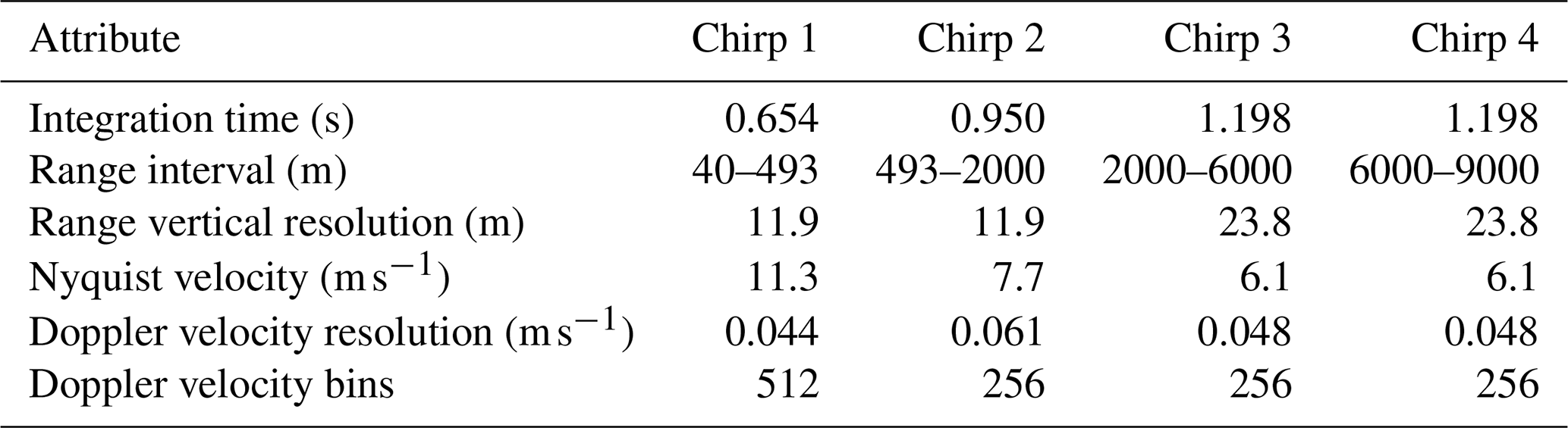
During CORSIPP, LIMRAD94 was mounted on a novel cold-temperature scanning unit, also manufactured by RPG. LIMRAD94 was deployed at an altitude of 2905 m at the Rocky Mountain Biological Laboratory (RMBL) about 525 m away from the second ARM Mobile Facility (AMF2) in Gothic (CO) near the RMBL Ore House between 15 November 2022 and 5 June 2023. LIMRAD94 observations were collected at constant elevation of 40° and an azimuth of 151° (towards the VISSS, AMF2 and the CSU X-band radar). The temporal resolution of LIMRAD94 data is about 3 s. Further technical details on the deployment of LIMRAD94 and VISSS during CORSIPP can be found in Kalesse-Los et al. (2023). The technical details of the radar chirp program employed during CORSIPP are listed in Table A1. For SAIL, the ARM KAZR (Widener et al., 2012) and a scanning dual polarization X-band radar (CSU X-band) from Colorado State University (CSU) were deployed in a distance of 525 m (at 151° azimuth and 2889 m a.s.l.) and 8018 m (at 149° azimuth and 3147 m a.s.l.), respectively, from LIMRAD94 (also see the Appendix, Table B1 and Fig. B1). From the CSU X-band radar data, RHI scans at 329° azimuth (towards the AMF2 and LIMRAD94) and plane position indicator (PPI) scans at 4° elevation were used in this study. In the appendix, Sect. B we also briefly discuss the volume matching of the CSU X-band radar and LIMRAD94 data.
2.1.1 Polarimetric radar data
LIMRAD94 is capable of measuring spectrally resolved polarimetric variables like differential phase shift and differential reflectivity, among others. Polarimetric calibration of LIMRAD94 was performed at the beginning of the field campaign during a time of vertical pointing measurements as described in Myagkov et al. (2016a).
The differential phase shift (ΦDP, °) consists of a backscatter and a propagational part as given by
where δ(°) is the backscatter differential phase that occurs due to non-spherical hydrometeors large enough relative to the radar wavelength such that the scattering is in the non-Rayleigh regime (Trömel et al., 2013). The specific differential phase shift (KDP, ° km−1) is the range derivative of the propagational component of ΦDP. Hence, to accurately calculate KDP, δ needs to be estimated and subtracted from ΦDP first. The estimation of δ in rain was thoroughly discussed in Trömel et al. (e.g., 2013); Myagkov et al. (e.g., 2020). However, for most frozen hydrometeors, δ was found to be negligible in the S, C, and X-bands (Balakrishnan and Zrnic, 1990; Ryzhkov et al., 2011; Trömel et al., 2013). In spectrally resolved ΦDP data, δ can be detected by a sudden increase or decrease of ΦDP in parts of the Doppler spectrum. Consequently, also integrated ΦDP often reveals characteristic “bumps” if δ is present (Trömel et al., 2013). During the case study presented, we checked integrated and spectral ΦDP for the above mentioned signs of δ that may impair the interpretation of KDP signatures. However, we found δ during our case study to be negligible. For LIMRAD94 and CSU X-band, the KDP was calculated from ΦDP using a convolution with low-noise Lanczos differentiators with window length of 23 gates. This method provides results that are analogue to a moving window linear regression and is implemented in the python package wradlib (Heistermann et al., 2013).
KDP depends on the shape, orientation, concentration, density and the size of ice particles. High concentrations of dense particles with more anisotropic shape and uniform orientation cause high KDP values. In rain, KDP is proportional to the 3rd power of the particle size (KDP ∼ D3). In low density snow, KDP is proportional to the 1st power of the particle size (KDP ∼ D1) due to density of snow being inversely depended on the diameter (ρ ∼ D−1). As the degree of riming increases, the proportionality of KDP shifts towards a higher power of the particle size, reflecting changes in the snow density. However, the influence of riming on KDP is contradictory: while riming increases the density of particles and hence KDP, riming also makes particles more spherical reducing KDP (Ryzhkov and Zrnic, 2019). KDP is also influenced by turbulence through its dependency on the width of the canting angle distribution (σ) via the orientation factor (F0), which is a function of σ (Ryzhkov et al., 2002; Ryzhkov and Zrnic, 2019). The canting angle is defined as the angle between the projection of a symmetry axis of a spheroidal particle and the vertical axis onto the polarization plane (Ryzhkov et al., 2002). If the canting angles of particles in a population differ a lot, the width of the canting angle distribution increases. The stronger the turbulence, the larger σ, the smaller F0 and hence the smaller KDP.
The differential reflectivity (ZDR, dB) is commonly defined as
where ZeH (mm6 m−3) is the equivalent radar reflectivity measured at horizontal polarization and ZeV (mm6 m−3) is the equivalent radar reflectivity measured at vertical polarization. At W-band, the largest contribution to positive ZDR values (in the ice phase) is usually made by the most dense anisotropic ice, small enough to be in the Rayleigh scattering regime, usually located on the slow edge of the Doppler spectrum. Contrary to KDP, ZDR is immune to the total concentration factor, so the combined analysis KDP and ZDR can be helpful to decouple effects of shape and concentration. Larger, strongly rimed, or aggregated hydrometeors, typically located on the fast side of the Doppler spectrum, are more spherical and exhibit low ZDR. Since ZDR is reflectivity-weighted, its magnitude is often reduced by the influence of these larger, spherical particles (e.g., Oue et al., 2018). To use ZDR without suffering from this masking effect, we also calculate the maximum spectral ZDR value () for each Doppler spectrum. As demonstrated in Von Terzi et al. (2022), this parameter is efficient for detection of small non-spherical particles masked by presence of large, more spherical particles like aggregates. Similar to KDP, ZDR is depend on σ (Hubbert and Bringi, 2003; Ryzhkov and Zrnic, 2019) and hence also decreased by turbulence. is furthermore decreased by turbulence through the broadening of the Doppler spectrum. Imagine that only one type of particle in a radar volume, moving with a certain terminal fall velocity, produces ZDR larger than zero. is high because the positive ZDR is measured at one certain Doppler velocity bin. If the fall velocity is now determined by turbulent air motion rather than the particles inherent terminal fall velocity, the particles producing the positive ZDR are “distributed” over a larger range of Doppler velocities and the ZDR at one certain Doppler velocity bin decreases. It is therefore essential to consider turbulence before interpreting any KDP or ZDR signatures.
LIMRAD94 was measuring at 40 ° elevation, which will cause ZDR and also KDP to be smaller than at lower elevation angles (e.g., Myagkov et al., 2016b). This should be taken into account when comparing the bulk values with other studies using ZDR and KDP but at different elevation angles.
2.2 VISSS
The first-generation VISSS was installed next to the AMF2 facility, in the line of sight of LIMRAD94 with a horizontal distance to LIMRAD94 of approximately 550 m (Fig. 1). VISSS1 has a pixel resolution of 58.832 µm px−1, a frame rate of 140 Hz, and an observation volume of () mm3 (Maahn et al., 2024). This yields an observational volume of 0.000339 m3. VISSS level2match variables (see Fig. 2 in Maahn et al., 2024) used in this study include particle size distributions (PSD), D32, complexity (c) and total number concentration (Ntot) and slope of the PSD (Λ). Following (Maahn et al., 2024), the complexity c is derived from the ratio of the particle perimeter p to the perimeter of a circle with the same area A :
The slope parameter of the PSD (Λ) is derived using the definition of Maahn et al. (2015):
where N0 is the intercept parameter of the exponantial PSD.
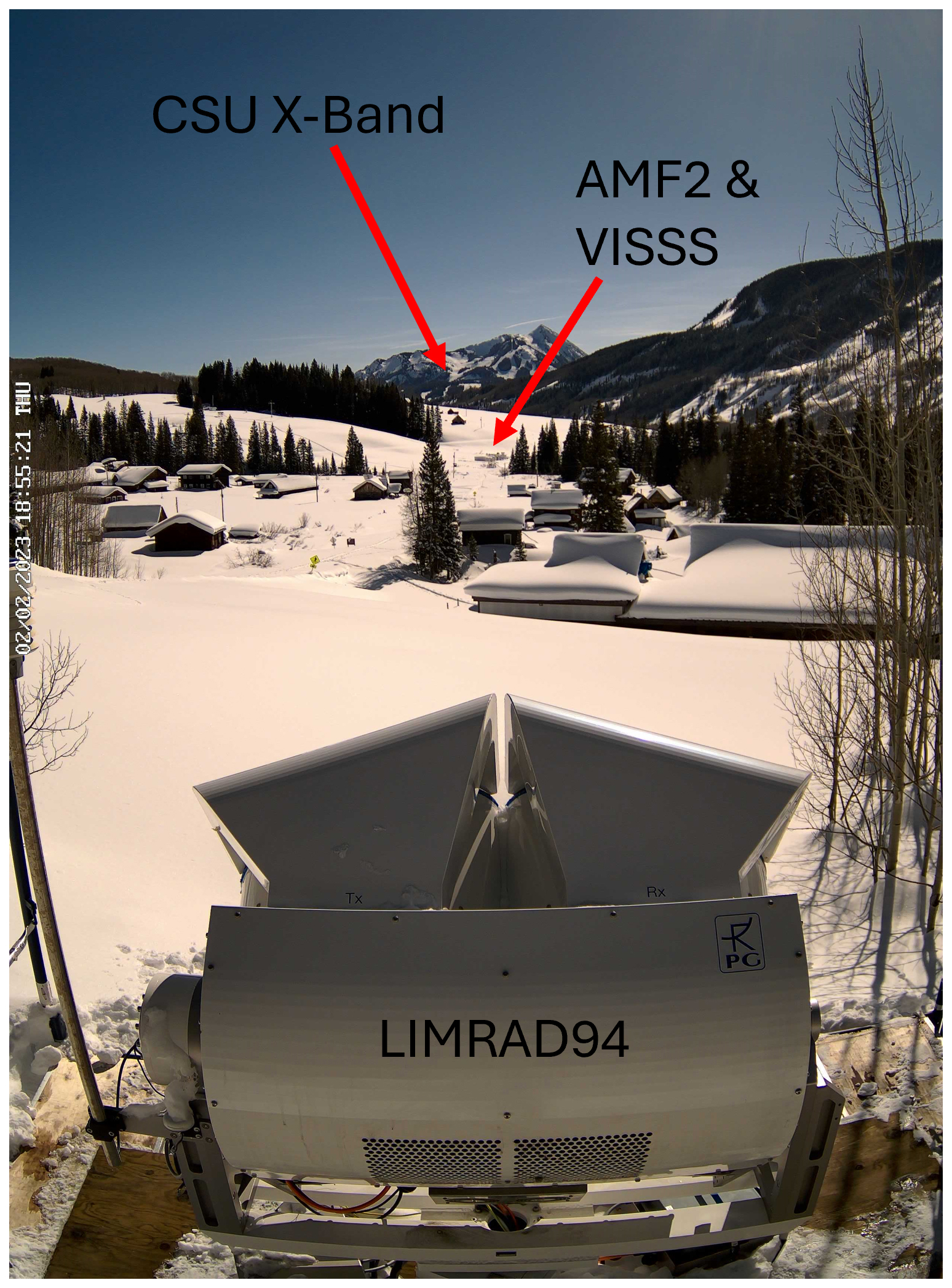
Figure 1Field of view of LIMRAD94 during CORSIPP pointed at 151 ° azimuth. The red arrows mark the locations of AMF2, VISSS and the CSU X-band.
D32 is the ratio of the third to the second measured PSD moment. Assuming that particle mass is proportional to the particle maximum dimension squared, D32 is a proxy for the mass-weighted mean diameter of the particle population (Maahn et al., 2015). Complexity is derived from the ratio of the particle perimeter to the perimeter of a circle with the same area (Maahn et al., 2024). The total number concentration reaches values of over 100 L−1 in this case study, which may seem unusual at first when comparing to other literature. VISSS is however more sensitive to small particles than laser disdrometers as shown by Maahn et al. (2024). This is likely the reason for the observed particle concentrations. All diameters used refer to the maximum diameter (Dmax), unless otherwise specified.
2.3 Additional products
During our study, we used additional data acquired at the AMF2 such as 2 m temperature, pressure, relative humidity, and wind speed as well as ARM 3-channel microwave radiometer liquid water path (LWP) and integrated water vapor (IWV); a detailed list can be found in the code and data availability section. Vertical temperature profiles on site are provided by the ARM interpolated sonde and gridded sonde VAP (Fairless et al., 2021). The sounding data, collected on site through two radiosonde launches per day (11:00 and 23:00 UTC) is transformed into continuous daily files with 1 min time resolution and combined with ARM 3-channel microwave radiometer temperature data.
2.4 Modeling of radar observables
To interpret radar observations and constrain quantitative estimates of the microphysical properties of ice particles, scattering simulations are employed.
2.4.1 T-matrix
The first approach approximates the shape of a particle as a spheroid and simulates its backscattering and forward scattering properties using the T-matrix scattering model (Mishchenko, 2000), hereafter referred to as the T-matrix approach. For a given wavelength, this method requires only three parameters: the equivolumetric diameter, the axis ratio, and the refractive index. The refractive index, which depends on the fraction of ice and air (Oguchi, 1983), can be adjusted to model ice particles with varying ice densities (Myagkov et al., 2016b). For simplicity, we assume the horizontal alignment of ice particles, albeit acknowledge that a broader distribution of canting angles generally leads to less pronounced polarimetric signatures. The T-matrix approach is computationally efficient; however, it is most applicable when the particles are smaller than the radar wavelength. Large ice particles, which tend to have highly irregular shapes, are not well-represented by the spheroidal approximation, particularly for short radar wavelengths. This limitation makes the T-matrix approach less suitable for modeling the scattering of rimed particles and aggregates at millimeter wavelengths (Leinonen et al., 2012; Kneifel et al., 2015).
2.4.2 DDA
For simulating the scattering of large ice particles at millimeter wavelengths, the Discrete Dipole Approximation (DDA) is often employed. This method allows for an accurate approximation of the scattering properties of individual particles with arbitrary shapes. However, DDA is computationally intensive and requires detailed specifications of the particle geometry which is generally unknown. Here, we randomly selected 105 unrimed dendritic aggregates from the snowScatt database (Ori et al., 2021), spanning maximum dimensions of 100 µm to 4 cm. As the falling behavior of snowflakes is determined by the complex interactions between aerodynamical and gravitational forces and is further complicated by, e.g., turbulence, we assume that the snowflakes fall with their maximum extension oriented horizontally. The DDA for the dendritic aggregates was calculated using adda (Yurkin and Hoekstra, 2011) at 94 GHz and 40 ° elevation, and averaged over 16 azimuth orientations.
2.4.3 Rationale for the applicability of scattering models
The primary aim of employing scattering models in this study is to identify the types of ice particles that contribute to the observed KDP signatures, rather than to establish a retrieval method. Since the T-matrix approximation uses spheroids, a clear relation between the ratio and the size and aspect ratio of the spheroid for a fixed apparent ice density is possible. While this approach is simplified, it yields sufficiently accurate results for preliminary conclusions, particularly when the particles are smaller than the radar wavelength, where the accurate mass distribution inside of the simulated particle is not as important as when particle size and wavelength become comparable. As for DDA we use more detailed shapes, fixing the effective density is not possible and such a clear relationship can not be found. Further, we do not have precise information about the size or shape of the observed particles. We therefore applied the spheroidal approximation and T-matrix model at X-band, the lowest frequency available in our campaign with a collocated measurement volume, to assess the sensitivity of KDP and Ze to particle size and aspect ratio (Sect. 3.3). This analysis also aids in determining whether KDP signatures are predominantly generated by larger particles. Conversely, the T-matrix method produces larger errors at W-band frequencies, where the shorter wavelength means non-Rayleigh scattering effects and the accurate description of the mass distribution in the particle become relevant (e.g., Ori et al., 2021, and references therein). This is especially true for particles with a low density, such as aggregates. Describing an aggregate with a soft spheroid is problematic, as the effective density in the spheroid needs to be small to accurately match the size and mass of the aggregate. This causes the (polarimetric) scattering properties of aggregates to be underestimated by soft spheroid methods such as the Tmatrix (e.g., Ori et al., 2021). Consequently, to estimate KDP and Ze at W-band for the particles detected with the VISSS, particularly concentrating on dendrite aggregates, we opt to use DDA computations (Sect. 3.4).
2.5 Fall streak tracking
Hydrometeor populations are influenced by horizontal and vertical winds as they precipitate to the surface and are hence exposed to advection. To estimate their microphysical evolution and to link ground observations with radar measurements aloft, these hydrometeor populations need to be observed along slanted fall streaks in vertical radar measurements. The analysis of the fall streaks is mostly achieved by reconstructing the advection using the present wind measurements (Marshall, 1953; Kalesse et al., 2016; Pfitzenmaier et al., 2017). As no sufficiently high-resolution wind data are available for our case study, we decided to analyze fall streaks with the simple approach of following maximum Ze values backwards from surface to cloud top. Specifically, the Ze at the start point is compared to the median Ze of the next three higher range gates. The time difference between two neighboring range gates is not allowed to exceed where Δh is the height difference in m between the range gates and vt is the mean Doppler velocity (MDV) measured by KAZR. The maximum Ze is chosen as the next point along the fall streak, and the process is repeated. This iterative process determines the suspected course of the fall streak in time and height. We acknowledge that horizontal homogeneity has to be assumed, especially for slanted measurements. Because the main wind direction in our case study is westerly but the radar is pointing southeast, it is obvious that we will never observe the exact same particles along their way to the ground.
2.6 Turbulence eddy dissipation rate retrieval (EDR)
Turbulence plays a critical role in understanding the evolution of hydrometeor populations and the behavior of polarimetric radar variables. The EDR is used as a proxy for turbulence. EDR is the rate at which turbulence kinetic energy dissipates in the atmosphere (Foken and Mauder, 2024). High EDR values indicate a more turbulent environment. We calculated EDR from the KAZR MDV for five minute time intervals, using the approach described in Vogl et al. (2024). To mask turbulence, we applied an empirical threshold of 0.001 m2 s−3 similar to the one found by Vogl et al. (2022). Note that the radar beams of KAZR and LIMRAD94 during CORSIPP were not aligned, so the measurement volume from which EDR is retrieved has a horizontal displacement from the LIMRAD94 measurement volume. This distance increases with increasing height.
First, we show a statistical comparisons of VISSS Ntot and LIMRAD94 KDP (Sect. 3.1). A case study with four KDP fall streaks is shown in (Sect. 3.2). For this case study, we present a combination of T-matrix KDP modeling and collocated CSU X-band observations in (Sect. 3.3) and KDP simulations using DDA based on VISSS data (Sect. 3.4).
3.1 KDP vs VISSS statistics
One advantage of the CORSIPP dataset is the close proximity of in situ observations by VISSS and detailed polarimetric W-band measurements of LIMRAD94. To understand how KDP is related to properties of the PSD, we compare KDP measurements of LIMRAD94 to VISSS surface measurements of Ntot and D32 for the period 1 December 2022 to 28 February 2023. LIMRAD94 KDP was spatially averaged (median) between 100 and 500 m above ground (52 range gates) to reduce effects of the measurement error, for the horizontal displacement of the two measurement volumes and for inhomogeneities in the observed precipitation. LIMRAD94 KDP was also temporally averaged (median) to match the VISSS time resolution of one minute. To compensate for the vertical displacement of the measurement volumes of VISSS and LIMRAD94 and the resulting time lag, LIMRAD94 data were shifted backwards in time as precipitation would be first visible in LIMRAD94 measurements and later in the VISSS. Given that the center of the averaged height is 300 m and assuming a terminal fall velocity of 1 m s−1, we chose five minutes as value for the time shift. We also tested time shifts of 3 and 10 min; none of them significantly changed the overall data distribution (not shown). Negative KDP values and range gates with SNR < 10 dB were excluded. LIMRAD94 data were only used if all range gates between 100 and 500 m contained data.
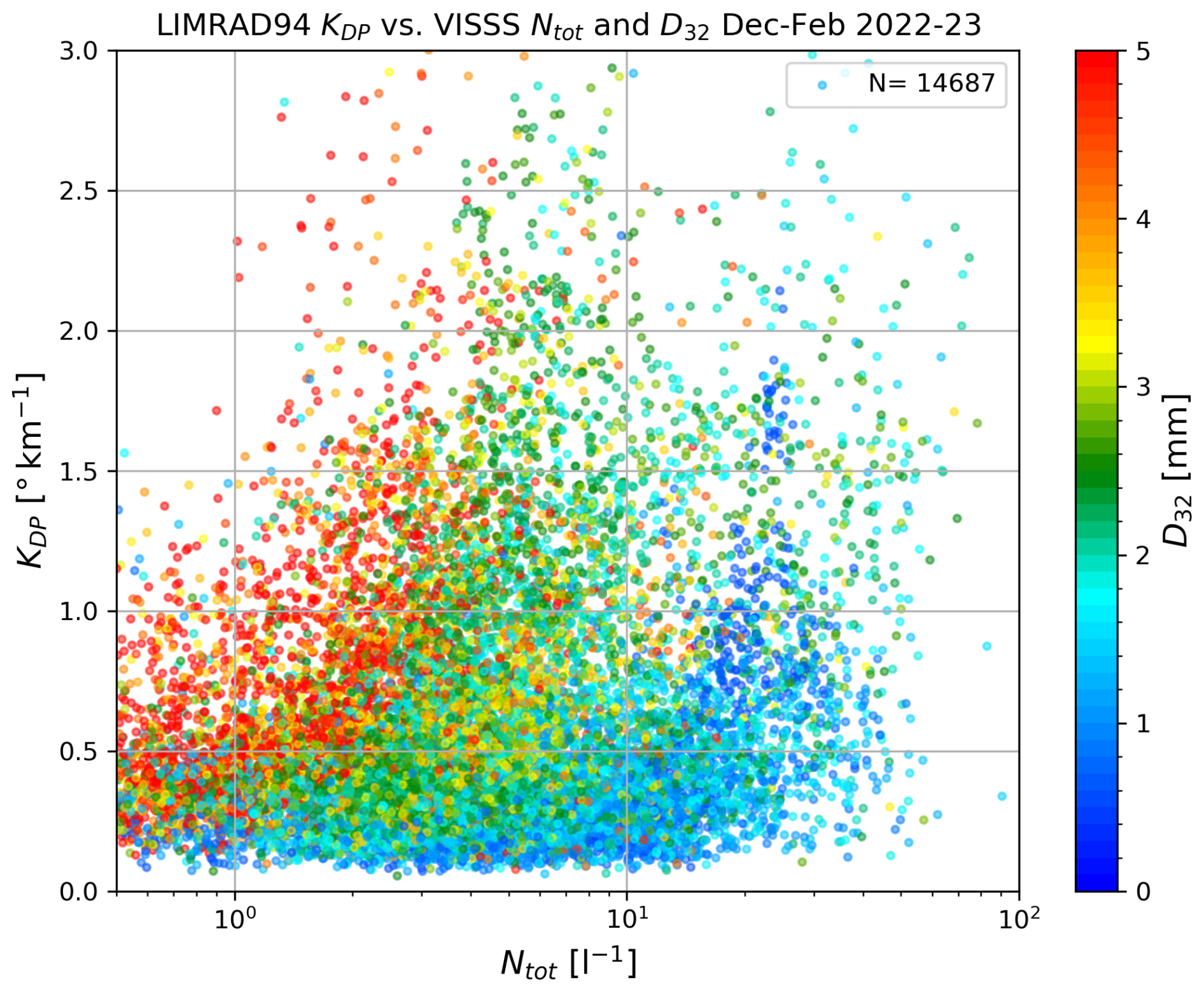
Figure 2Scatterplot of LIMRAD94 KDP vs. VISSS Ntot for DJF 2022/23. The x-scale is logarithmic. LIMRAD94 KDP was spatially averaged between 100 and 500 m above ground and temporally averaged to fit the VISSS time resolution of one minute. Colors show D32 of the respective PSD. A total of 14 773 data points (14687 min) were used for the plot.
Overall, a clear connection between higher KDP and Ntot is evident. Particle populations with D32 below 2 mm (blueish dots in Fig. 2) reach higher Ntot up to 100 L−1 more frequently. Within these particle populations, higher KDP values of up to 2 ° km−1 are mostly linked to Ntot greater than 10 L−1. In contrast, particle populations with D32 of 4 mm or higher (red dots in Fig. 2) mostly occur when Ntot is below 10 L−1, but can also result in KDP values larger than 2 ° km−1. Particle populations with low Ntot and high D32 mainly form through aggregation, which decreases the overall Ntot by reducing the amount of smaller particles while increasing the mean particle diameter. There are three possible explanations for the KDP produced by these particle populations:
-
The larger aggregates are the main contributors to the observed W-band KDP.
-
The small ice particles are the main contributors to the observed W-band KDP while their number concentration is anti-correlated with the presence of large aggregates.
-
Large aggregates and small ice particles contribute to the observed KDP, their relative contributions depends on the particle size distribution and the properties of the particles.
The possible contribution of larger aggregates to increased W-band KDP was recently discussed in Von Terzi et al. (2022). Since KDP does not suffer from the non-Rayleigh effects as Ze and ZDR, it can keep increasing with particle size as long as the shape is somewhat preserved (Lu et al., 2015; Von Terzi et al., 2022). Especially early-stage aggregates can be reasonably assumed to be still highly non-spherical and contribute substantially to the ensemble KDP signal (Moisseev et al., 2015).
3.2 Snowfall case study: 6 December 2022
To investigate the formation of KDP signatures and the influence of different microphysical processes and particle sizes on KDP, we chose the case study on 6 December 2022. Over a span of 1.5 h, we identified and analyzed four fall streaks (FS1–4) characterized by enhanced KDP. Despite exhibiting similar KDP magnitudes, VISSS revealed varying particle population properties within these fall streaks.
3.2.1 Synoptic discussion
6 December 2022 featured a complex synoptic situation with a stationary front over the Colorado Rocky Mountains and a surface low developing along this front over eastern central Colorado, slowly moving southward during the day. The measurement site was influenced by the development of this surface low. An overview of surface meteorological variables and the vertical wind profile during the case study is given in Fig. 3. Just before 15:00 UTC we observed a sudden change in 2 m wind direction from southwesterly to northerly winds, an increase in 2 m wind speed from under 2 to over 5 m s−1 (Fig. 3b) and a decrease in 2 m temperature and humidity (Fig. 3c). After 15:00 UTC, we saw a steady increase in surface pressure (Fig. 3b). The evolution of the surface meteorological variables in Gothic points to a cold front passage just before 15:00 UTC (see the magenta lines in Fig. 3). The wind throughout the lower troposphere up to 3000 m above LIMRAD94 was from the southwest before the cold front with a slight veer and an increase in speed toward higher altitudes, indicating the advection of warm air (Fig. 3a). With the passage of the cold front, the wind turned to westerly and later northwesterly directions up to 1500 m above LIMRAD94. Aloft, the winds backed to the southwesterly direction again, indicating cold air advection. LWP and IWV decreased with the passage of the cold front (Fig. 3d), indicating that a dryer air mass being advected. The nature of the precipitation changed during the cold front passage; from low Ntot, low Λ, and high D32 precipitation dominated by aggregates and comparably low number of small particles before the cold front to a high Ntot, high Λ and low D32 precipitation with very mixed particle types (see Fig. 4e). Therefore, we especially focus on this time period between 14:30 and 16:30 UTC in our case study.
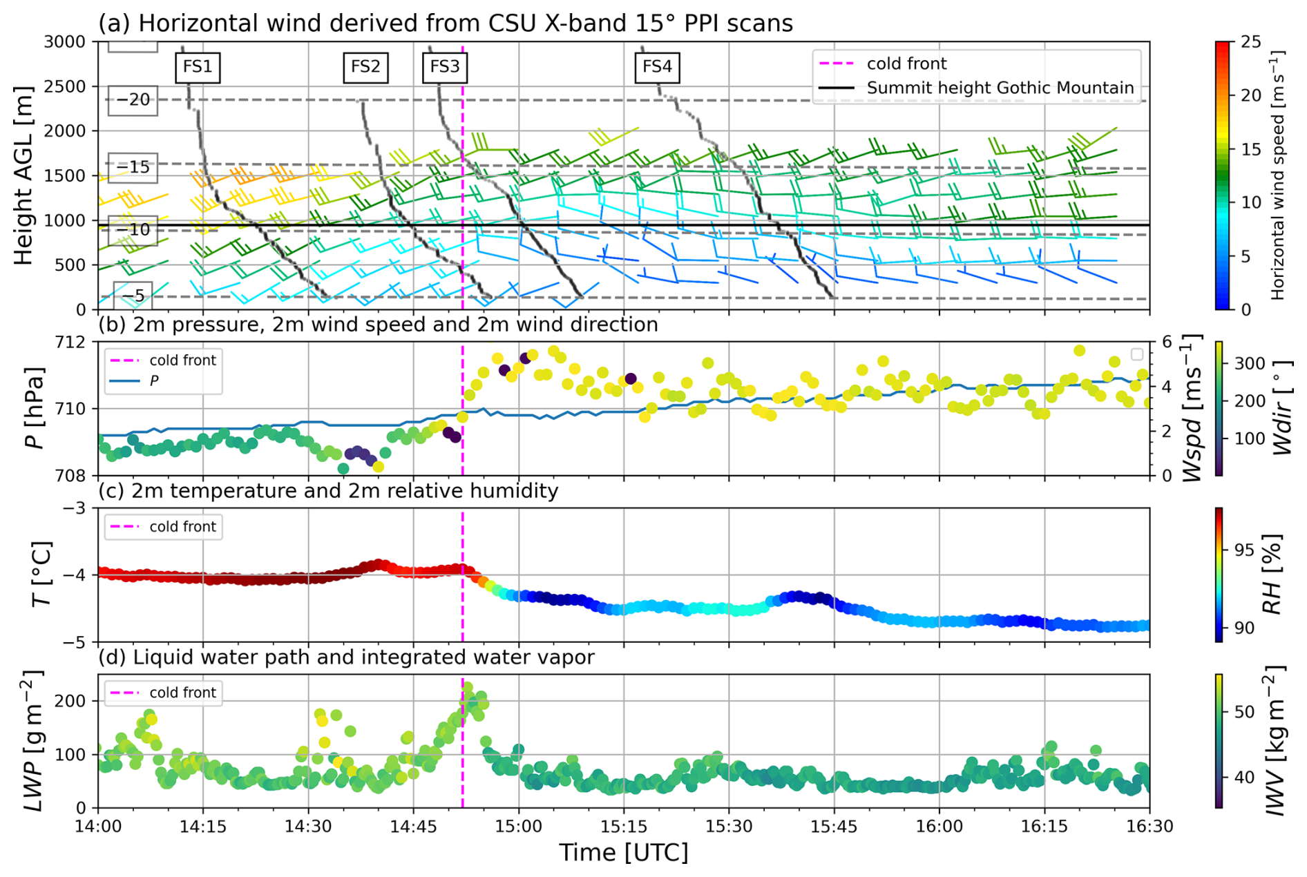
Figure 3Meteorological observations during the case study on 6 December 2022. The vertical dashed magenta line in all plots indicates the passing of a cold front. (a) Horizontal wind speed and direction. Horizontal grey dashed lines represent air temperature (°C) from the interpolated radiosonde product. The analyzed fall streaks are displayed as black lines with their respective labels. The black solid horizontal line denotes the height of Gothic Mountain. (b) AMF2-based meteorological variables at 2 m: pressure, wind speed and direction as color code. (c) AMF2-based 2 m temperature and relative humidity. (d) AMF2-based MWR, LWP, and IWV.
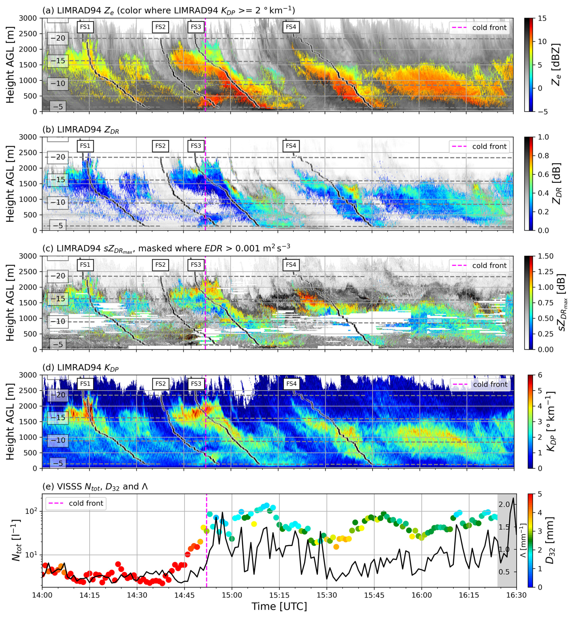
Figure 4LIMRAD94 time–height plots during the case study on 6 December 2022. Analyzed fall streaks shown as black lines with labels. In every panel except (d), data are only colored where LIMRAD94 KPD > 2 ° km−1. The remainder of the Ze and observations where KDP was below this threshold are displayed in black and white. Grey lines are isotherms. (a) Ze. (b) ZDR. (c) with areas masked where EDR exceeds the turbulence threshold of 0.001 m2 s−3. (d) KDP. (e) Minutely VISSS Ntot on the y axis and Λ (black line) plotted against time on the x axis. Colors are the respective D32 values.
3.2.2 The turbulence layer
Radar variables observed by LIMRAD94 as well as VISSS Ntot, Λ and D32 throughout the case study are shown in Fig. 4. Due to the orography surrounding the measurement site, we observed a distinct layer of enhanced turbulence, mostly at and below 1000 m above ground level (a.g.l.). This is visualized by the EDR-masked data (white where EDR exceeds 0.001 m2 s−3) in Fig. 4c).
The main wind direction above 1000 m a.g.l. was southwest before the cold front and west to northwest after the cold front passage (Fig. 3a). The inner valley flow was weak southwesterly before the cold front and moderate northerly after the cold front (Fig. 3b). Hence, the wind shear was enhanced along the interface between the blocked valley and the cross-barrier flow aloft, which would lead to shear-induced turbulence as explained in Ramelli et al. (2021). The main blocking feature west of Gothic is Gothic Mountain (3850 m). The height of the summit of Gothic Mountain above the location of LIMRAD94 (roughly 1000 m a.g.l.) corresponds well to the top of the observed turbulence layer.
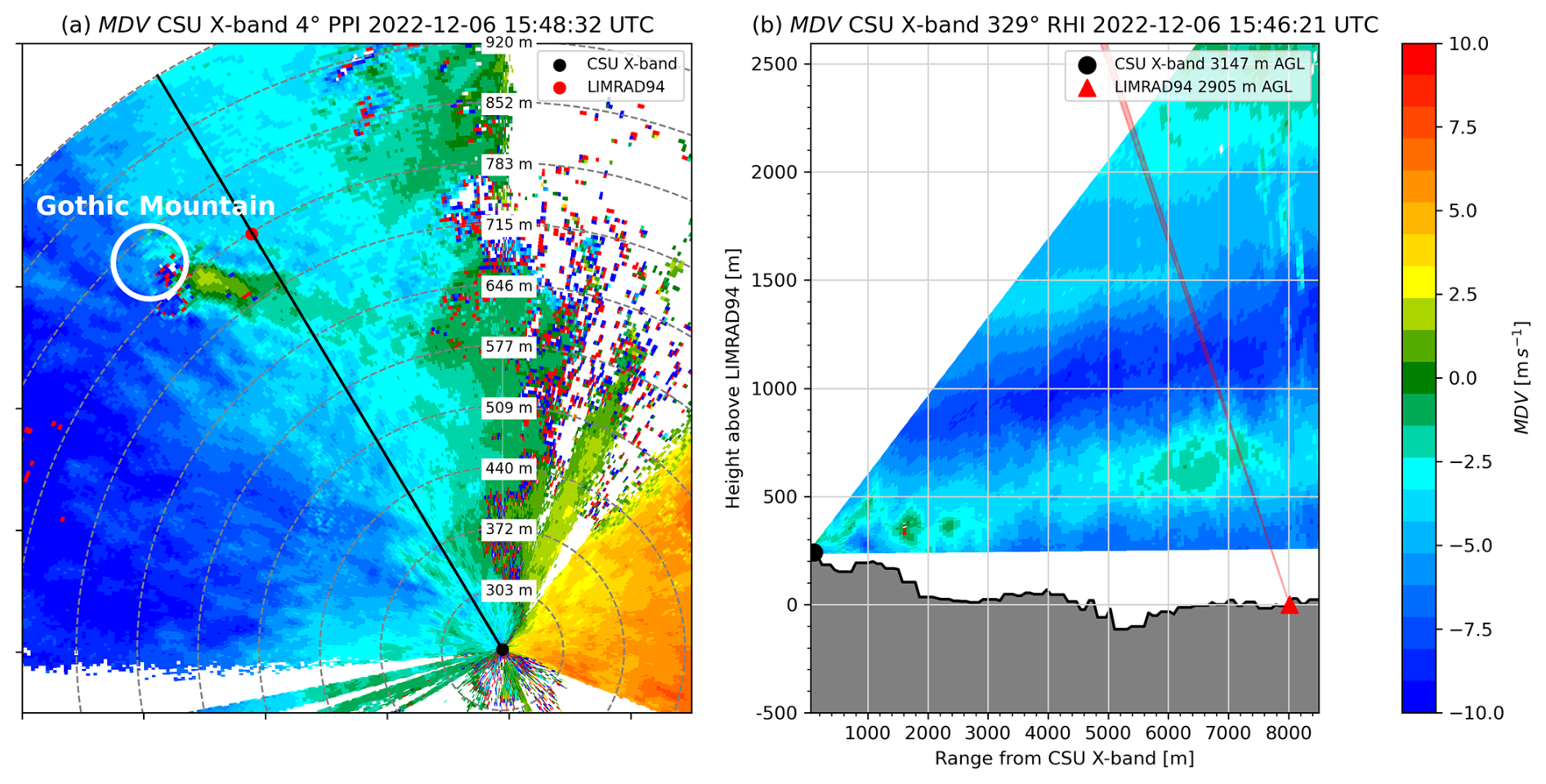
Figure 5(a) Mean Doppler velocity (approx. radial component of horizontal wind) of the CSU X-band PPI scan at 4 ° elevation angle with location of Gothic Mountain (white circle) and direction of RHI scan at azimuth 329 ° (black line) at 15:48:32 UTC on 6 December 2022. Grey dashed circles are placed at every 1000 m range from the CSU X-band. Labels are the respective heights above LIMRAD94 of the CSU X-band radar beam. (b) Mean Doppler velocity of the CSU X-band RHI scan (azimuth 329 °) at 15:46:21 UTC on 6 December 2022 with LIMRAD94 beam direction (red). Grey shading shows the elevation profile.
Figure 5 shows the MDV of the CSU X-band from a PPI (a) and a RHI (b) scan at around 15:48 UTC and 15:46 UTC, respectively. During that time, EDR indicates enhanced turbulence between 500 and 1200 m a.g.l. (Fig. 4c). The MDV measured during the PPI scan can be approximated as the radial component of the horizontal wind. Negative values (blue) in Fig. 5 correspond to motion towards the radar, positive values (yellow-red) to motion away from the radar. The PPI is partly blocked by mountains, however the westerly wind is apparent by blue colors west of the CSU X-band and orange-red colors to the east. Where MDV is close to zero, the wind is perpendicular to the radar beam. Downstream of Gothic Mountain, there is a small corridor where the MDV values turn positive in sharp contrast to the surrounding negative values. This implies that downstream of Gothic Mountain, the wind turns to more southerly directions. The effect diminishes quickly further downstream. In the RHI scan (Fig. 5b), the southerly wind component is visible by the area of more green colors in the 6000–7000 m range from the CSU X-band and between 400 and 1000 m above LIMRAD94. This area of lee-induced flow disturbance (termed ALIFD) could be partly caused by a counterflow, indicative of a blocked low-level flow, as, for example, described in Ramelli et al. (2021). Along the edges of the ALIFD, wind shear is enhanced which could lead to the observed turbulence. The beam of LIMRAD94 is shown in Fig. 5b) as a red cone, and it is apparent that the measurements of LIMRAD94 are impacted by the turbulence in and around the ALIFD.
3.2.3 Evolution of polarimetric variables along fall streaks (FS)
In the following sections, the development of W-band polarimetric variables along the four fall streaks of enhanced KDP before, during, and after the cold front are analyzed in detail. VISSS images of hydrometeors during the fall streaks and the respective PSD are shown in Figs. 6 and 7, respectively. The polarimetric radar observations during the four selected fall streaks (FS1-4) are shown in Fig. 8. All subplots in Fig. 8 have the same structure, showing profiles of KDP, Ze, , ZDR, spectral width (SW) and correlation coefficient (ρhv) as a function of the temperature. Fall streaks were derived as explained in Sect. 2.5. A grey line was added for every height/temperature where EDR exceeded 0.001 m2 s−3. SW of LIMRAD94 was added to the plots as an additional proxy for turbulence (as for example done in Majewski et al., 2023). For each of the analyzed fall streaks, we will try to assess which particle types and microphysical growth processes lead to the observed KDP signatures and how they are influenced by turbulence.
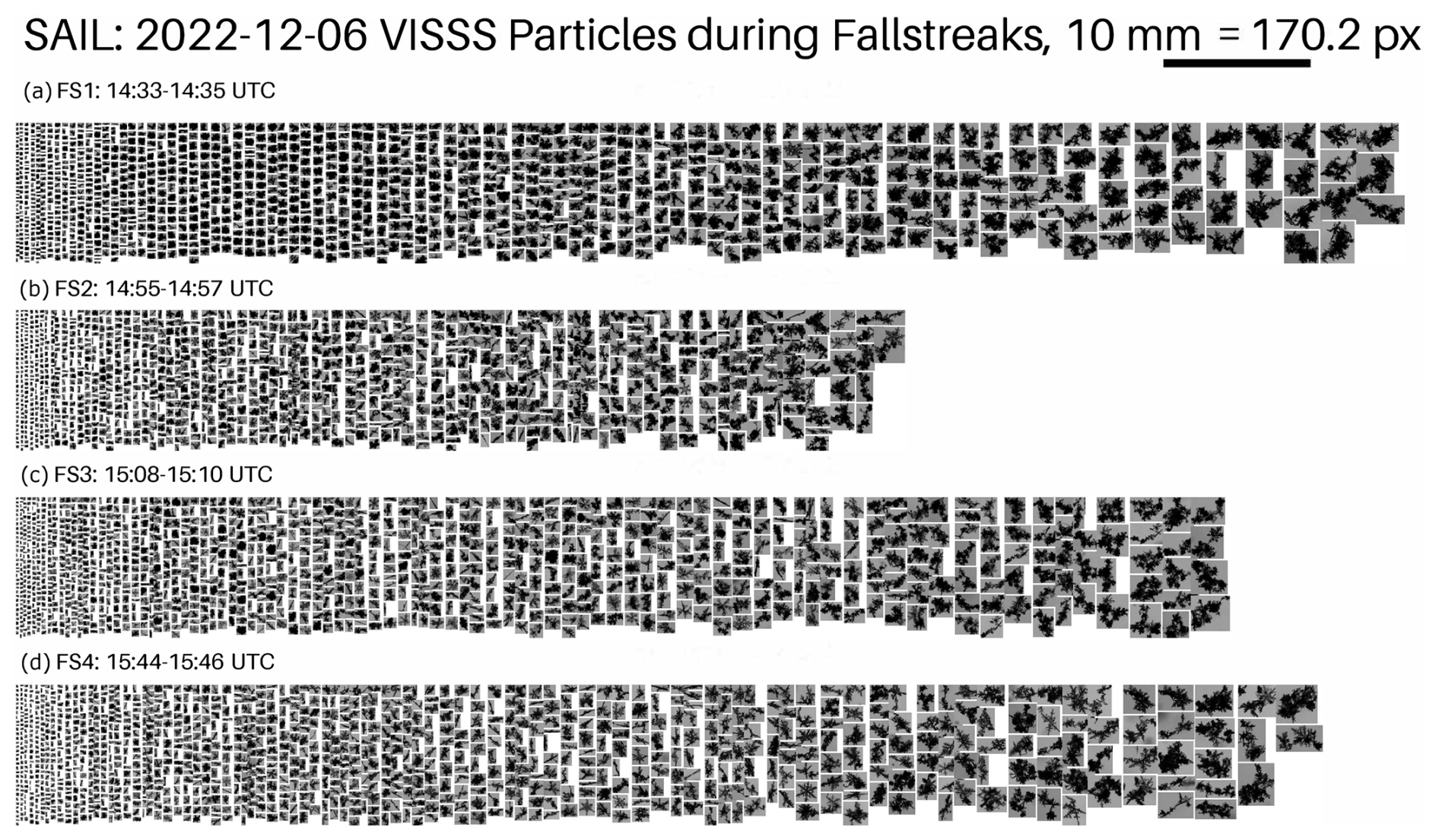
Figure 6Particles observed on the ground by VISSS during the four fall streaks. For each fall streak, 3 min of data are displayed. Particles were divided into size bins and a fixed number of particles is displayed for each bin (if the bin contains a sufficient number of particles). The number of displayed particles is decreasing with increasing particle size.
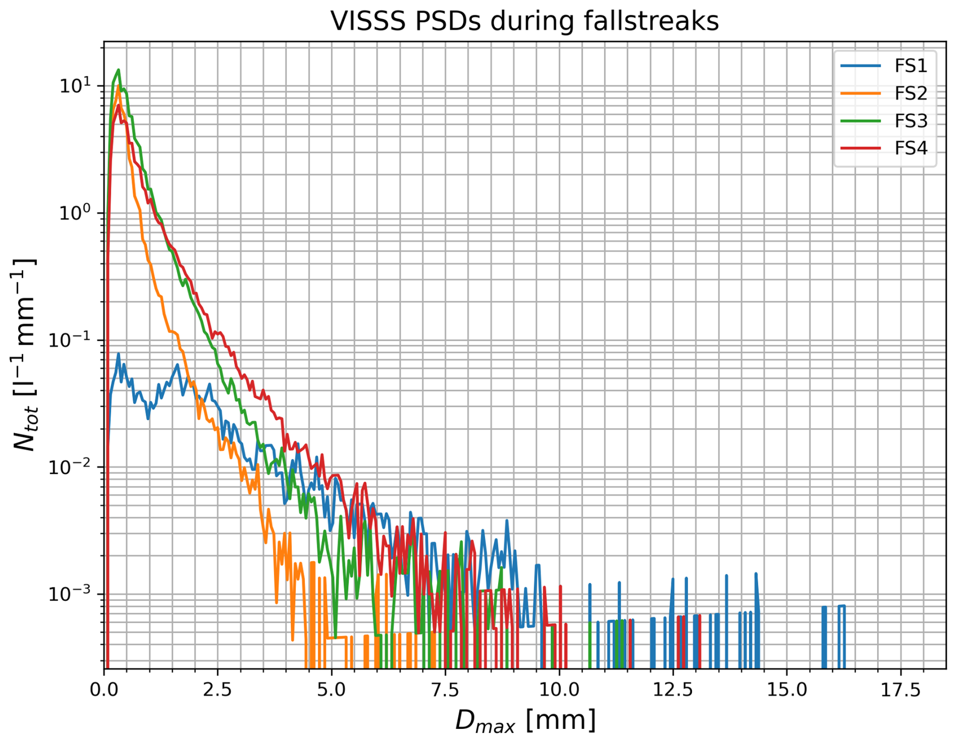
Figure 7VISSS PSDs (one minute averages) observed during the times when the four selected fall streaks reached the surface.
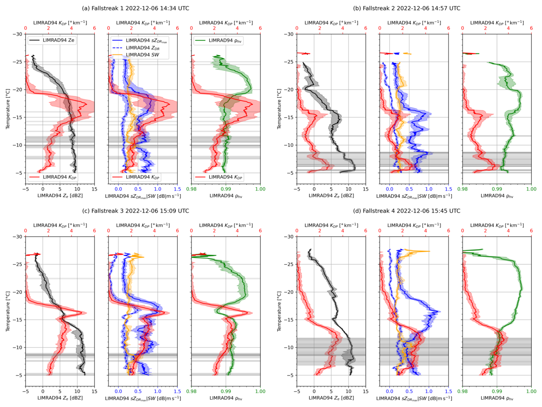
Figure 8Profiles of polarimetric variables along the FS1 (a), FS2 (b), FS3 (c), and FS4 (d). Profiles of KDP (red), Ze (black), (blue), spectral width (orange), and ρhv (green) are plotted against the temperature. All polarimetric variables were averaged (median) for ±2 min around the fall streak track (solid lines). Colored shaded areas mark 25/75th percentile values of the respective variable. Grey shaded areas mean that the EDR exceeded the turbulence threshold of 0.001 m2 s−3.
Before the cold front (FS1)
The first KDP fall streak (FS1) we analyze appears around 14:15 UTC, originating in the DGL at around 2300 m a.g.l. and temperatures between −20 and −15 °C (Fig. 4d). It reaches the ground well before the cold front at around 14:30 UTC. Before the cold front passage, the dominant particle type is aggregates, smaller heavily rimed or graupel-like particles were also observed by the VISSS (see Fig. 6a). Before 14:45 UTC, Ntot is always below 10 l−1 and D32 is around 4–5 mm (Fig. 4e), indicating that the particle population at the surface contains larger particles (see also Fig. 7). A low Λ (Fig. 4e) of around 0.5 mm−1 further suggests a PSD with a reduced number of smaller particles, which is also visible in Fig. 7).
The polarimetric variables along FS1 are shown in Fig. 8a). At temperatures colder than −20 °C, KDP is close to zero and rather low with values around 0.25 dB. ZDR is slightly negative with −0.2 dB. The negative ZDR observed above the DGL is most likely caused by differential attenuation within the DGL. Differential attenuation at W-band by ice is either related to large particle number concentrations, high mass densities, or a combination of both (Liao et al., 2008). ρhv in this upper part of FS1 is high with values above 0.995. This combination of ZDR, KDP and ρhv suggests that the particle population is rather uniform and consists either of nearly spherical particles, particles with a low effective refractive index, or a combination of the two (e.g., Andrić et al., 2013).
As these particles fall into the DGL, they experience depositional growth through enhanced supersaturation over ice. and ZDR increase because depositional growth in the DGL promotes anisotropic shape enhancement (e.g., Andrić et al., 2013; Takahashi, 2014). The sharp decrease in ρhv together with the difference in and ZDR could be linked to a secondary particle mode consisting of freshly formed, anisotropic particles is often observed in the DGL (described in Sect. 1). starts to increase at around −20 °C to values of around 0.75 dB (center panel in Fig. 8a). The 99th percentile of during the 2.5 h of our case study is 1.32 dB, so 0.75 dB is still comparably small. The comparably low in the DGL during FS1 indicates either more spherical, less dense or smaller anisotropic particles. Collocated with the maximum and ZDR, we see a sharp increase in KDP (Fig. 8a) to over 6 ° km−1). Following the hypothesis of Griffin et al. (2018) described in the Introduction, the peaks of low ZDR and high KDP in FS1 between −20 and −15 °C could be caused by a high concentration of I-type particles. If I-type particles enter the DGL, they will experience rapid depositional growth because of the enhanced supersaturation over ice. Larger particles will grow slower and mostly maintain their shape, while smaller I-types will grow faster and could serve as embryos of rapid growing D-type particles (e.g., Sheridan et al., 2009; Griffin et al., 2018). The existing water vapor would be distributed over a large number of particles, which, as we speculate, would result in overall lower supersaturation and cause the newly formed D-type particles of larger quantities to grow into overall lower diameters and lower density. So while ZDR could be masked by more spherical I-type particles, in FS1 could be low because of D-type particles with an overall smaller diameter. At the same time, these particles are more numerous, which enhances KDP and causes a collocation of the maximum and KDP. This theory would imply that the closer the maxima in KDP and are in height, the higher the overall number concentration of particles in the upper DGL. Another potential cause of the observed radar signatures could be additional SIP at the upper part of the DGL as, e.g., suggested in Andrić et al. (2013) and Von Terzi et al. (2022). A large number of I-type particles with a wider size distribution would also enhance the likelihood of ice collisional fragmentation, providing even more embryos for the growth of D-type particles. A second, smaller peak of KDP at around −15 °C in FS1 could be caused by additional dendritic growth at this temperature. A similar structure of KDP in the DGL was for example shown in simulations by Andrić et al. (2013), caused by dendritic growth at this temperature. At temperatures warmer than −15 °C, we see an overall decrease in KDP towards the ground with a collocated moderate increase of Ze, a signal commonly attributed to the aggregation of anisotropic particles into less dense, more spherical shapes and the reduction of Ntot (e.g., Andrić et al., 2013; Trömel et al., 2019; Von Terzi et al., 2022; Hu et al., 2024).
The summit height of Gothic Mountain is roughly located around the −10 °C isotherm. Turbulence is found at this height (Fig. 8a). Just above the turbulent layer, we see an increase in together with a small peak in KDP. A similar signature of enhanced ZDR above a turbulent layer was found by Hogan et al. (2002); Grazioli et al. (2015). They explained that SLW and ice splinters are transported upward by updrafts and grow into anisotropic particles. In our case, the splinters would grow into D-type particles given temperatures between −10 and −15 °C which might explain the enhanced and KDP. Below the turbulent layer, we find that and also KDP increase slightly again while ZDR remains almost constant. LWP up to 200 g m−2 (see Fig. 3d) during FS1 enables riming, and graupel is detected by VISSS (see Fig. 6 FS1). The enhanced and KDP could be attributed to graupel–snowflake collisions, which are known to produce anisotropic ice fragments with sizes up to 2 mm (Grzegorczyk et al., 2023). In the first stage of riming, only the density of particles increases without changes in density of shape (Erfani and Mitchell, 2017), which might also cause the observed increase in and KDP below the turbulent layer. The PSD observed by VISSS during the time FS1 reaches the surface shows a comparably low number of small particles (Fig. 7) together with the presence of larger aggregates (see Fig. 6 FS1). Aggregation likely causes a rapid depletion of small particles near the surface, thereby reducing Ntot. The low Λ observed in Fig. 4 provides additional evidence that small particles are depleted in the PSD.
During the cold front (FS2)
With the passage of the cold front at the surface, we see a distinct increase in Ntot in the VISSS measurements from less than 10 L−1 to around 100 L−1 (Fig. 4e). At the same time, D32 (colors in Fig. 4e) decreases to around 2 mm and Λ increases to nearly 2 mm−1, indicating smaller particles are dominant in the measurement volume. Compared to FS1 before the cold front, the VISSS PSD in FS2 (Fig. 7), shows an overall increase/decrease in particles smaller/larger than 2 mm, respectively. The sudden increase in the number of small particles could be caused by blowing snow, which is supported by multiple observations. As the hours before the cold front featured conditions with weak 2 m winds and large aggregates, loose snow on trees or the ground was likely lifted along the convergence of the surface cold front and behind it by the suddenly increased northerly wind. KAZR data during the case study are shown in Fig. 9. The lift associated with the cold front can be seen as positive KAZR MDV (i.e., upward motion) in Fig. 9b. The strongest upward motion was observed at around 14:52 UTC in the lowest 500 m along the surface convergence. The low-level uplift provided by the cold front supports the theory that blowing snow was lifted and kept elevated in the vicinity of the surface convergence. In the presented case, blowing snow could also be detectable at higher altitudes because it is lifted off the higher valley slopes and advected over the lower valley floor. Figure 9a shows the KAZR Ze together with the 0 m s−1 isotach (red line). Between 14:50 and 14:55 UTC and roughly between 250 and 900 m a.g.l., there is an area of enhanced Ze with no connection to a FS, supporting the idea of Ze-enhancement caused by blowing snow.
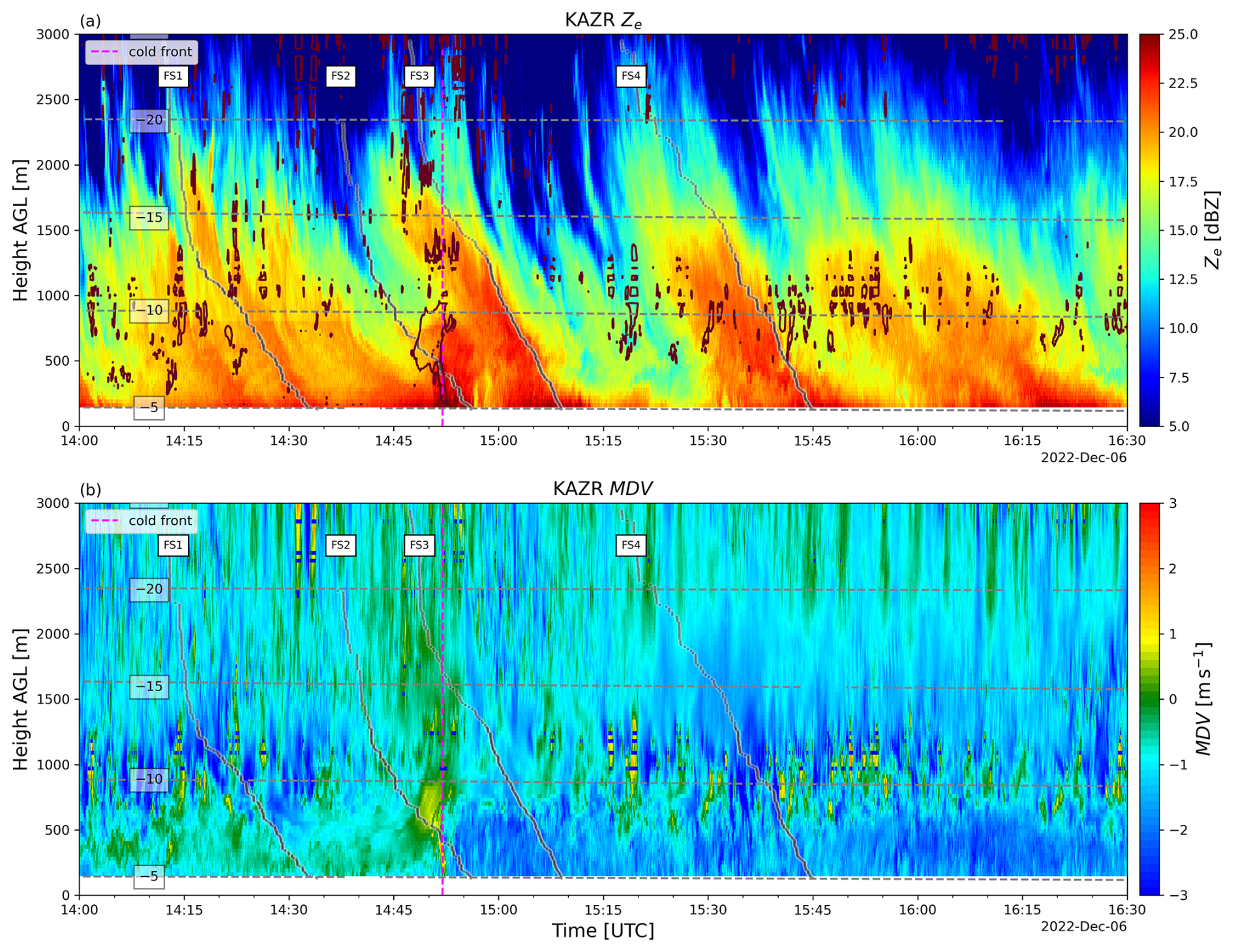
Figure 9Time–height plots of KAZR MDV (a, c) and KAZR Ze (b, d) of the 6 December 2022 case study. The red contour in panels (b) and (d) marks the 0 m s−1 isotach. Dashed grey lines in panel (b) and (d) mark the isotherms (°C) with respective labels. The analyzed fall streaks retrieved from LIMRAD94 measurements are displayed as black lines with their respective labels. Note that these fall streak paths do not exactly match the KAZR Ze because of the horizontal displacement of the measurement volumes.
Between 14:50 and 14:55 UTC, we also see a small area of enhanced LIMRAD94 KDP in the lowest 500 m (Fig. 3b). Figure 8b shows a possible fall streak track during the time of the cold front passage. FS2 displays a sudden change in the polarimetric variables and hence likely the particle mode when entering the pocket of cool and dryer air between −8 and −5 °C (Fig. 8b). The boundary between the two air masses is marked by an increase in turbulence (Fig. 8b). Below the top of the turbulent layer, and KDP decrease sharply which could however be due to a turbulence masking effect. Within the turbulent layer, KDP then increases again downwards to values of up to 3 ° km−1 at the lower edge of the turbulent layer. Assuming that KDP is still masked by turbulence, the true KDP values without turbulence would be much higher. Ze also increases by about 5 dBZ within the turbulence layer, its peak value is collocated with the KDP peak. We conclude that this KDP signature is likely caused by blowing snow.
At the top of the turbulent layer, we also see an increase in together with a small peak in KDP, similar to FS1. The explanation could again be small ice splinters being transported upward by updrafts (Hogan et al., 2002; Grazioli et al., 2015). Ice splinters could originate either from SIP processes inside the turbulent layer or from lifted blowing snow. At temperatures between −5 and −8 °C the splinters can grow into columns or needles (Bailey and Hallett, 2009). Indeed, some needles were observed by the VISSS for FS2 (Fig. 6b).
After the cold front (FS3, FS4)
FS3 forms between 14:45 and 15:00 UTC at around 2000 m and reaches the ground around 15:10 (FS3). FS4 forms between 15:25 and 15:35 UTC at 1500–2000 m and reaches the surface just after 15:45 UTC (FS4). The surface relative humidity (RH) decreases noticeably before each fall streak reaches the ground (Fig. 3c) and increases when the FS reaches the ground. At the same time, surface Ntot increases (Fig. 4e). This could point to drier air that is advected behind the cold front, which is moistened again by the sublimation of precipitating snow.
FS3 originates in the upper dendritic growth layer (DGL) at around 2000 m and temperatures between −15 and −20 °C. The maximum KDP values in the DGL reach 5 ° km−1 (Fig. 8c), which is slightly lower than in FS1. The peaks of and ZDR have values of around 1 and 0.5 dB, respectively which is higher than in FS1. Comparing Ze at −20 °C in FS1 and FS3, we find Ze to be about 6 dBZ in FS1 and 2 dBZ in FS3. Assuming that the size of I-type particles is similar in both FS, this would point to a lower concentration of I-type particles sedimenting in the DGL in FS3 and thus less I-types serving as embryos for D-type growth. This in turn would lead to larger D-type particles (since the existing water vapor is distributed over fewer particles) with larger (and higher ZDR due to less masking) and still in a sufficiently high number concentration to produce high KDP.
In FS3, the increase in and KDP coincides with a sharp decrease in ρhv (Fig. 8c) which quickly recovers near −15 °C, while KDP experiences a sudden drop of approximately 2 ° km−1. This signature could indicate rapid aggregation or riming, processes typically associated with an increase in Ze. However, during the KDP decrease, Ze also shows a slight decline. This behavior may reflect the limitations of interpreting a three-dimensional system with two-dimensional data. Between −15 and −12 °C, Ze increases strongly, indicating a possible increase in particle diameter which might point to aggregation. In the same T-range, KDP is nearly constant with high values of around 3 ° km−1. This points to the formation of new anisotropic particles in parallel to the aggregation process, which continues to enhance the number concentration and hence keeps KDP constant. Nevertheless, it is not ruled out that aggregates contribute to the magnitude of the KDP in this part of FS3.
The whole area of enhanced KDP around the black line marking FS3 between 14:40 and 15:00 UTC reveals another interesting feature: inside the area of high KDP values, a horizontal gradient in Ze, ZDR and is visible (Fig. 4a–d). ZDR and are especially low on the left side of black line marking FS3 while KDP exceeds 4 ° km−1. Following the hypothesis of Griffin et al. (2018), this might point to I-type particles seeding in the DGL in parts of the fall streak and dominating the particle population. ZDR might additionally be masked by more spherical, low density aggregates. The presence of these larger aggregates could also explain the higher Ze on the left side of FS3. On the right side of FS3, higher and ZDR might be caused by the presence of dense, anisotropic D-type particles. The lower Ze and less masked ZDR might be related to the absence of large aggregates.
Below the turbulent layer in FS3, KDP decreases, but still has values of 2–2.5 ° km−1 until the fall streak reaches the surface, while Ze increases slightly towards the surface (Fig. 8c). Where KDP decreases between −10 and −7 °C, we also see an increase in ρhv which might point to enhanced aggregation due to the turbulent layer as for example observed by Chellini and Kneifel (2024). The observation of graupel, dendrites, and many dendrite fragments by VISSS (see Fig. 6c) points to frequent graupel–snowflake collisions. These collisions were found to produce up to 500 fragments per collision (Grzegorczyk et al., 2023). The fragment size distributions of such collisions revealed a mode at around 0.4 mm in their study. In the PSD measured by VISSS (Fig. 6 FS3), particles with a Dmax of less than 0.5 mm were the most frequently observed. A portion of these particles might be fragments of graupel–snowflake collisions, which could also explain the very high Ntot of around 110 L−1 at the surface during FS3.
In FS4 (see Fig. 8d), we find a very prominent peak in of 1.25 dB between −17 and −13 °C. Contrary to the previous fall streaks, this peak is firstly occurring much further above the KDP peak and secondly has higher values than in FS1 and FS3. No collocated ZDR signature exists, which can only mean that the ZDR signature is completely masked by larger spherical particles. This fits to the theory of Griffin et al. (2018): only very few and large D-type particles are present and produce high , while KDP is negligible due to their low number concentration. At T warmer than −15 °C, decreases while Ze and KDP increase. This signature might point to the early stage formation of D-type aggregates. If there was a layer of SLW at the top of the turbulent layer as mentioned by Grazioli et al. (2015), it is also possible that the dendrites from above become rimed, forming even graupel. The resulting velocity gradient in the PSD would favour collisions and hence collisional breakup. Resulting splinters would quickly grow into anisotropic ice crystals, enhance the number concentration and therefore KDP. However, our data does not allow a definitive conclusion about the origin of this polarimetric signature.
Between around 1200 m and 500 m a.g.l. corresponding to −12 and −7 °C, FS4 is influenced by the turbulent layer (Figs. 4c and 8d) which is also evident in Fig. 9b) as strongly fluctuating MDV layer. In general, in FS4 the turbulent layer is more pronounced than during the previous fall streaks leading to a decrease in and ZDR as well as an increase in SW. KDP is rather homogeneous throughout FS4 inside the turbulent layer, horizontally and vertically. A decrease near the ground is only seen in the lowest 200 m. It seems likely that the constant KDP is caused by increased ice collisional fragmentation that keep the number concentration of anisotropic particles high throughout the turbulent layer. VISSS images at the time of FS4 shows a wide mix of particles, many dendrite branches, aggregates in various stages of riming, and some graupel (see Fig. 6d). This confirms that ice collisional fragmentation and riming are likely major processes inside the turbulent layer. This is consistent with the findings of Ramelli et al. (e.g., 2021); Chellini and Kneifel (e.g., 2024). Similar to FS3, the ice collisional fragmentation in the observed turbulent layer might be the reason for the high Ntot of 100 L−1 during FS4.
3.3 Estimating particle size responsible for W-band KDP signatures using T-matrix simulations and CSU X-band Ze and KDP observations
In the previous section, we discussed the fingerprints of microphysical processes influencing polarimetric radar variables and hypothesized about the particles responsible for the observed KDP. Here, we use T-matrix simulations and CSU X-band radar observations to constrain the sizes of particles contributing to KDP signatures in the observed fall streaks. Instead of using LIMRAD94 data, the ratio of KDP to Ze at X-band is analyzed, as its Ze is not affected by non-Rayleigh scattering for particle diameters smaller than 10 mm.
T-matrix simulations were performed to calculate the ratio of KDP to Ze at X-band for artificial spheroidal particles with varying aspect ratios. These calculations used Ze in linear units (mm6 m−3). Since both KDP and Ze are proportional to the concentration of particles, the ratio of these radar variables is therefore independent of the concentration. The ratio is thus mostly sensitive to size and shape of ice particles. The ratio decreases with an increase in particle diameter, because in snow, Ze and KDP are roughly proportional to the 4th and 1st power of the particle's size, respectively. Figure 10 shows the results of the T-matrix simulations, the logarithm of the ratio between KDP and Ze at X-band is plotted for different aspect ratios. Even though the KDP and Ze ratio depends on the aspect ratio of particles, it is suitable for roughly estimating the sizes of particles producing KDP signatures.
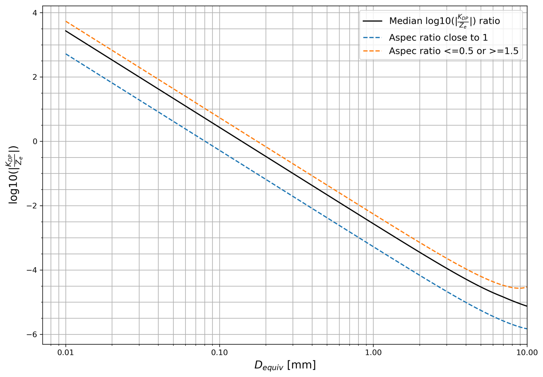
Figure 10T-matrix simulation results: Logarithm of the ratio between X-band KDP and Ze plotted for different aspect ratios and equivolumetric diameters (logarithmic x axis). The black line is the median ratio per Dequiv over all aspect ratios (0.5–1.5). The minimum ratio per Dequiv can be seen for aspect ratios close to 1 and is plotted as the blue dashed line. For aspect ratios 0.5 or ≥ 1.5 the ratio per Dequiv is higher (orange dashed line).
Figure 11Time–height plot of LIMRAD94 KDP for the 6 December 2022 case study. CSU X-band data are superimposed onto LIMRAD94 KDP when the latter ≥ 1.5 ° km−1. Colored squares: equivolumetric particle diameter retrieved from the logarithm of the ratio between X-band radar KDP and Ze for RHI scans. The analysed fall streaks as well as isotherms are indicated in grey.
To assess the observed ratios of KDP and Ze, we analyzed CSU X-band data within the KDP fall streaks (see Fig. 11). The CSU X-band KDP was divided by cos2 of the elevation angle to correct for the different elevation angles during the RHI scans (Ryzhkov and Zrnic, 2019). The Ze and KDP ratio was translated into Dequiv using T-matrix simulations shown in Fig. 10. Since the Ze and KDP ratio only slightly varies with the aspect ratio, we used the median value of the ratio for each Dequiv. The retrieved particle diameter ranges from 0.2 to 1.5 mm within the fall streaks. In the upper DGL, values tend to be less spread, ranging from 0.2 to 0.8 mm, while they increase up to 1.5 mm towards the surface which might be linked to the increasing particle size through aggregation and/or depositional growth (also see Fig. 13). In a few pixels, the simulated sizes exceed 1.5 mm.
In FS1, simulated particle sizes below 1000 m exceed 0.8 mm more frequently compared to the other fall streaks. This aligns with the observed VISSS PSD in FS1, which stands out from the others by exhibiting a greater abundance of large aggregates and fewer small particles (see Fig. 7).
Considering that during the fall streaks, VISSS showed mean mass-weighted diameters ranging from 1.5 to 5 mm, we conclude that the contribution of large ice crystals to KDP is small and a major part of the KDP signatures is produced by ice particles smaller than 0.8 mm in diameter in the DGL and smaller than approximately 1.5 mm closer to the surface.
The ratio of KDP and Ze depends on the absolute calibration of the CSU X-band. By comparing Ze of the CSU X-band with Ze from LIMRAD94 (not shown), we found a low bias of the CSU X-band of about 4 dB. This roughly agrees with a low bias of 2.6 dB found with an absolute target calibration of the CSU X-band performed pre-campaign. However, considering the several orders of magnitude range of the KDP to Ze ratios, even 4 dB offset would not significantly affect this analysis. In addition, we emphasize that the ratio alone is insufficient to estimate the exact size of particles when different populations of ice particles coexist within the same volume. To illustrate this, consider two populations of particles, such as large aggregates and small ice particles. The large aggregates primarily determine Ze due to their size, while the high concentration of small particles may dominate the KDP values. Thus, Ze and KDP effectively characterize different particles within the volume. Nevertheless, the ratio can still be used to constrain the maximum possible size of particles dominating the KDP values.
3.4 DDA simulations of W-band KDP based on VISSS data
Based on the results obtained from the analysis of the CSU X-band data, we expect that a major part of the KDP signatures at W-band are produced by small ice particles. To further investigate the possible contribution of large particles, a more detailed analysis is required. The T-matrix method is not applicable to W-band measurements because large particles may produce resonance effects. In such cases, the spheroidal approximation does not always adequately represent the scattering properties (e.g., Schrom and Kumjian, 2018). To test the possible contribution of larger aggregates to our observed LIMRAD94 KDP signatures, we calculated KDP and Ze based on VISSS in situ observations using DDA simulations. The observations of LIMRAD94 KDP and Ze are temporally averaged to 1 min and vertically averaged between 30 m (lowest range gate) and 400 m a.g.l. The ratio between observed and simulated KDP and Ze values at W-band are displayed in Fig. 12a/b (blue/black) solid line, respectively. For DDA simulations of KDP, only particles >=2.5 mm were used which we assume to be aggregates. We determined this size threshold based on images and the spectral complexity measurements from VISSS (not shown). The particles for the simulations were selected from the DDA database using a nearest neighbor regression, considering the nearest 5 particles and weighting them with their inverse distance to calculate the scattering properties expected for the in situ particle based on their maximum dimension. All of these particles were assumed to be dendrite aggregates, which fits the VISSS observations of particles larger than 2.5 mm.
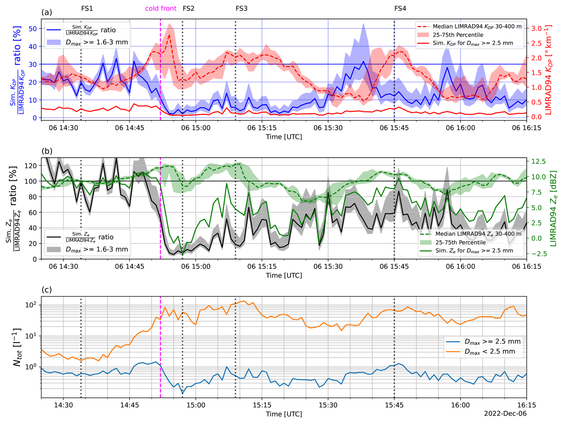
Figure 12(a) Median LIMRAD94 KDP between 30 and 400 m a.g.l. (red dashed line) with the 25–75th percentile (red shading) and ratio of DDA-based forward simulated KDP (Sim. KDP) to observed LIMRAD94 KDP (blue line). For the blue line, only particles with diameters ≥ 2.5 mm were used, the blue shading shows the range of the simulations when just particles ≥ 3 mm (lower edge) or ≥ 1.6 mm (upper edge) are included. (b) Median LIMRAD94 Ze between 30 and 400 m a.g.l. (green dashed line) with the 25–75th percentile (green shading) and ratio between DDA-based forward simulated Ze (Sim. Ze) and observed LIMRAD94 Ze (black line). For the black line, only particles with diameters ≥ 2.5 mm were used, the grey shading shows the range of the simulations when just particles ≥ 3 mm (lower edge) or ≥ 1.6 mm (upper edge) are included. In (c), VISSS particle number concentrations for particles with D >=2.5 mm (blue) and D<2.5 mm (orange) are shown. Magenta line marks the passage of a cold front while the black dotted lines mark the analyzed fall streaks.
Overall, the temporal evolution of the simulated KDP and Ze appears to match the observations quite well, except for the time during FS2 which is strongly influenced by blowing snow. During FS1, we see that the KDP ratio is about 20 %, which is the value that Von Terzi et al. (2022) found as contribution of larger aggregates to W-band KDP in their study. The simulated Ze is about 80 % to 100 % of the observed Ze. This is about the range we would expect, given that the PSD during FS1 contains a comparably low number of particles < 2.5 mm. This also underlines that even when the larger aggregates determine Ze, the smaller ice crystals still produce the majority of KDP without contributing much to Ze. This is consistent with our findings from the previous Sect. 3.3.
During the cold front in the vicinity of FS2, there is only a very low number of larger aggregates and KDP is mainly produced by small blowing snow particles as we explained in Sect. 3.2.3. Meanwhile, there are only few aggregates ≥ 2.5 mm (see the blue line in Fig. 12c), hence their contribution to Ze and KDP is very small. During FS3, the number concentration of aggregates ≥ 2.5 mm is similar to FS1, while the number of particles < 2.5 mm is about 2 orders of magnitude higher than during FS1. This might explain why the simulated Ze of particles ≥ 2.5 mm only explains 20 %–30 % of the observed Ze. The observed KDP is higher than during FS1 and the simulations suggest that larger aggregates contribute less than 10 % to the observed KDP. Right before and after FS3 we see a higher number of larger aggregates which may contribute up to 15 % of the observed KDP.
During FS4, the number of particles ≥ 2.5 mm is highest compared to the other fall streaks, while the concentration of the smaller particles is slightly lower than during FS3. The contribution of bigger particles to KDP is higher (around 15 %), while simulated Ze of these particles contributes about 80 % to 90 %, which seems reasonable.
In general, we conclude that a contribution to KDP of 10 %–15 % can be attributed to aggregates with a maximum diameter ≥ 2.5 mm. When the PSD contains a comparably large number of aggregates, we even see contributions of up to 20 % to KDP without overestimating Ze in the simulations. In this analysis we completely omit the effects of riming. If riming enhances the density of aggregates, KDP might be initially increased by an increase in density, provided that the aggregates maintain their anisotropic shape. The opposing effect of riming on KDP was briefly discussed in Sect. 2.1.1.
We presented results obtained from in situ snowfall camera (VISSS) measurements and collocated polarimetric Doppler W-band (LIMRAD94) observations collected within the CORSIPP project embedded within the framework of the Atmospheric Radiation Measurement (ARM) Surface Atmosphere Integrated Field Laboratory SAIL campaign (Feldman et al., 2023). LIMRAD94 KDP and additional polarimetric variables along four high-KDP fall streaks during a cold-front passage related snowfall case study on 6 December 2022 were analyzed and linked to VISSS observations. To evaluate which particles contribute to the observed KDP signatures, we further tried to constrain the particle sizes that contribute the most to the observed LIMRAD94 KDP using T-matrix simulations and collocated CSU X-band measurements. Lastly, we determined the amount of LIMRAD94 KDP likely produced by aggregates ≥ 2.5 mm using DDA simulations and VISSS in situ observations.
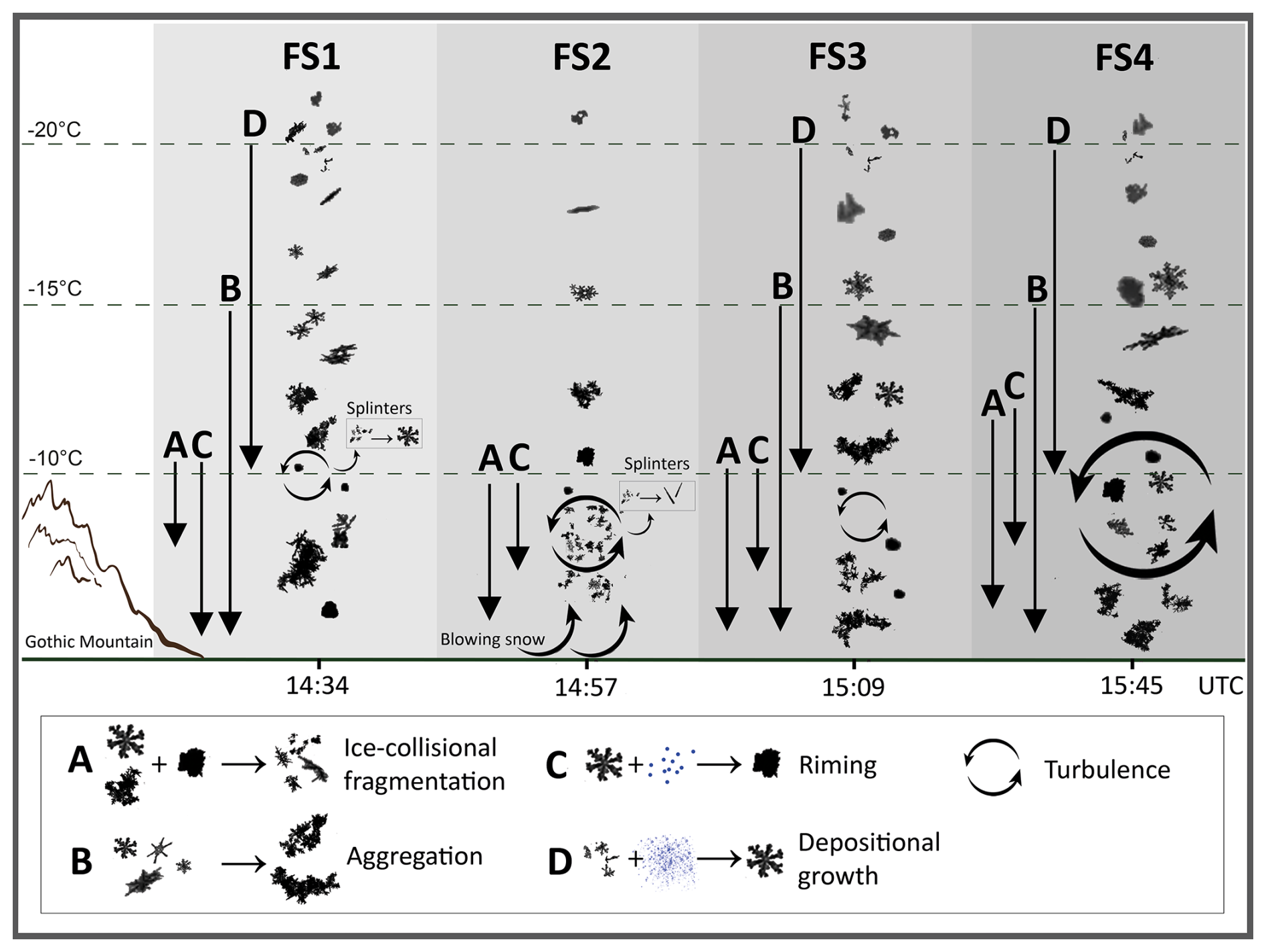
Figure 13The suspected dominating microphysical processes during the analyzed fall streaks FS1–FS4) we derived based on our observations. The black arrows show for which temperature interval we assume a certain mechanism (marked with the respective letter) to be dominant. Snow particle images from VISSS (during the time of each fall streak) were used to visualize the possible particle types in each fall streak.
To conclude our study, we would like to highlight the following key findings:
-
By combining in situ and remote sensing measurements, we found that at W-band, high KDP magnitudes are produced by a broad range of number concentrations (Ntot), ranging between 1 and 100 l−1 (see Sect. 3.1 and Fig. 2). Particle populations with Ntot below 5 L−1 often featured D32 above 5 mm, indicating that the PSD contains more large particles. We thus argue that when interpreting W-band KDP signatures, it should be kept in mind that similar W-band KDP values can be produced by strongly variable particle number concentrations.
-
Based on T-matrix simulations using a spheroidal approach and CSU X-band observations, we found that the main contributors to W-band KDP signatures in the analyzed the fall streaks was likely by ice particles with a diameter below 0.8 mm in the DGL and below 1.5 mm closer to the surface (see Sect. 3.3 and Fig. 11). DDA simulations of KDP based on VISSS PSDs during our analyzed the fall streaks show, that 10 %–15 %, in extreme cases up to 20 % of the KDP observed close to the surface during the fall streaks can be attributed to aggregates ≥ 2.5 mm (see Sect. 3.4 and Fig. 12). This agrees with the results of Von Terzi et al. (2022). Revisiting the three possible explanations for high KDP in particle populations with low Ntot and high D32 (Sect. 3.1), we conclude that small ice particles are the main contributors to the observed W-band KDP and up to one-fifth of the observed KDP can be attributed to large dendrite aggregates. When interpreting W-band KDP signatures, it should be remembered that the contribution of aggregates to W-band KDP is usually not negligible.
-
We identified blowing snow as another contributing source to increased KDP values during a cold front passage. Specifically, lifted blowing snow likely caused W-band KDP of up to 3 ° km−1 (see Sect. 3.2.3).
-
Turbulence, more specifically spectral broadening and the increase in the width of the canting angle distribution, significantly reduces the values of ZDR and KDP significantly. The magnitude of seems to be more affected by turbulence than KDP. Therefore, we conclude that it is essential to consider turbulence before interpreting any ZDR or KDP signatures.
-
Despite the dampening effect of turbulence mentioned above, we observed an increase in KDP inside a strong turbulent layer. The turbulent layer was caused by wind shear along the interface between the blocked valley flow and the cross-barrier flow aloft (see Sect. 3.2.2). VISSS observations measured below the turbulent layers revealed number concentrations of over 100 L−1. Due to high number of dendrite branches in VISSS observations, we suggest that this is caused by increased ice-collisional fragmentation that keeps the number concentration of anisotropic particles high throughout the turbulent layer and hence causes enhanced KDP. This SIP mechanism of enhanced ice-collisional fragmentation in the presence of turbulence was also found in the studies of Ramelli et al. (2021) and Dedekind et al. (2023). Few graupel particles coexisting with unrimed ice observed by VISSS likely further increased the collision efficiency (see Sect. 3.2.3). Furthermore, we found an increase in and KDP at the top of the turbulent layers during FS1 and FS2, as observed by Hogan et al. (2002); Grazioli et al. (2015).
-
ZDR, and KDP maxima of different magnitudes were well collocated in FS1 and FS3 and strongly displaced in FS4. This is likely linked to different concentrations of I-type and D-type particles as described in Griffin et al. (2018). When ZDR signatures were masked by bigger and more spherical particles, proved to be a very useful additional variable. We therefore emphasize the advantage of using both, integrated and spectrally resolved ZDR.
We have added a conceptual diagram (see Fig. 13) to provide an overview of the suspected dominant microphysical processes during the analyzed fall streaks, which we derived based on our observations.
During FS1, FS3, and FS4, we also hypothesized that early stage aggregates in the lower part of the DGL cloud have contributed to the observed W-band KDP (as, for example, already discussed in Moisseev et al. (2015)). This speculation seems reasonable, as we did show that dendrite aggregates can contribute up to 20 % to W-band KDP. However, in the observed case studies, the lower part of the DGL was about 1000 m a.g.l. Thus, early stage aggregates were not observed at the ground by the VISSS. Early stage aggregates in the DGL might have a different shape and other polarimetric properties. A topic of further investigation of the CORSIPP dataset could thus be the analysis of polarimetric signatures of early stage aggregates for cases where the lower edge of the DGL was nearly at ground level.
We do not in particular focus on the effects of riming in our modeling studies. Riming however may even increase the contributions of aggregates to KDP. In the early stages of riming, the density may be enhanced without an initial change in the particle shape (Erfani and Mitchell, 2017). KDP might therefore initially increase by an increase in density, provided that the aggregates maintain their anisotropic shape. This influence of riming on aggregate contribution to KDP may therefore be a topic of further investigation. Naturally, there are caveats when linking surface in situ observations to radar measurements. The observational volume of LIMRAD94, even at close range, is several orders of magnitude larger than the one of VISSS. This can be partly compensated for by temporal averaging and consideration of time shifts between the measurements, but generally requires us to assume some homogeneity in the precipitations.
The authors acknowledge that the measurement site is characterized by complex terrain and distinct synoptic forcing mechanisms. Consequently, the conclusions drawn are specific to this particular environmental and synoptic context and may not be generalizable to other settings.
In summary, this study highlights the complexity of interpreting W-band KDP in snow. We show that polarimetric W-band radar observations combined with surface in situ observations of snow PSD by the VISSS and radar forward simulations can give valuable insights into cloud and snowfall microphysical processes. Given the increasing use of polarimetric W-band radar observations and that even space-borne mission concepts have been proposed (Illingworth et al., 2018; Battaglia et al., 2022), the sensitivities of the polarimetric variables to microphysical properties should be further explored.
The chirp table used for the presented statistics and case studies is presented in Table A1.
The exact north alignment of LIMRAD94 was ensured by using a solar scan routine that is integrated into the LIMRAD94 software. The sun is a source of strong microwave radiation which can be detected by the passive 89 GHz channel of LIMRAD94. That way, the azimuth value at which the sun is visible in the measurements of LIMRAD94 is determined. The true azimuth of the sun is known from the GPS module on board LIMRAD94. The offset from the true north is then simply the difference between the two azimuth values. During the first months of CORSIPP, LIMRAD94 measurements were performed at a constant elevation (CEL) of 40 ° and an azimuth of 151 °. The field of view during the CEL measurements is shown in Fig. 1. The azimuth is chosen so that KAZR and VISSS are in the line of sight of LIMRAD94. The azimuth angle from LIMRAD94 towards CSU X-band is roughly 149 ° so there is a slight directional mismatch of both radar beams during the CEL measurements of LIMRAD94. The range height indicator (RHI) scans of the CSU X-band towards an azimuth of 329 ° overlap best with the beam of LIMRAD94 (Fig. B1). However, the beams of both radars overlap enough to compare the measurements. In order to make the RHI scans of the CSU X-band and the CEL measurements of LIMRAD94 comparable, the closest range gates were selected for each time step. With increasing altitude, hence the elevation angle of the CSU X-band, the horizontal distance of the closest range gates increases. The maximum horizontal distance is 120 m, the vertical distance does not exceed 8 m (Fig. B2). Coordinates and relative locations of all of the instruments can be found in Table B1.
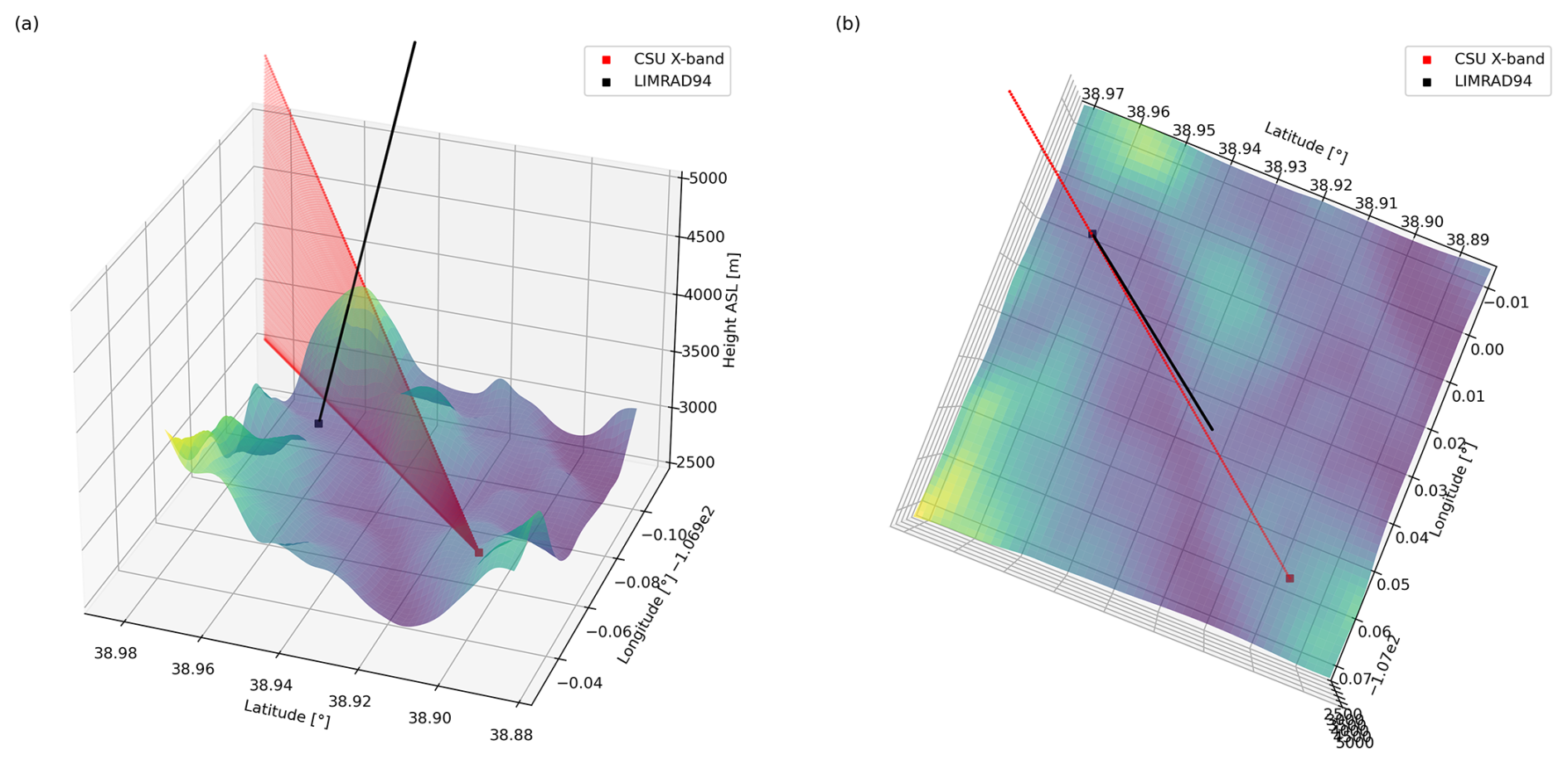
Figure B1Radar beam overlaps of LIMRAD94 and CSU X-band RHI scan (azimuth 329 °) from side view (a) and top view (b). The red lines represent the CSU X-band radar beam and black lines the LIMRAD94 radar beam. The size of the actual radar volume is not accounted for in the plot.
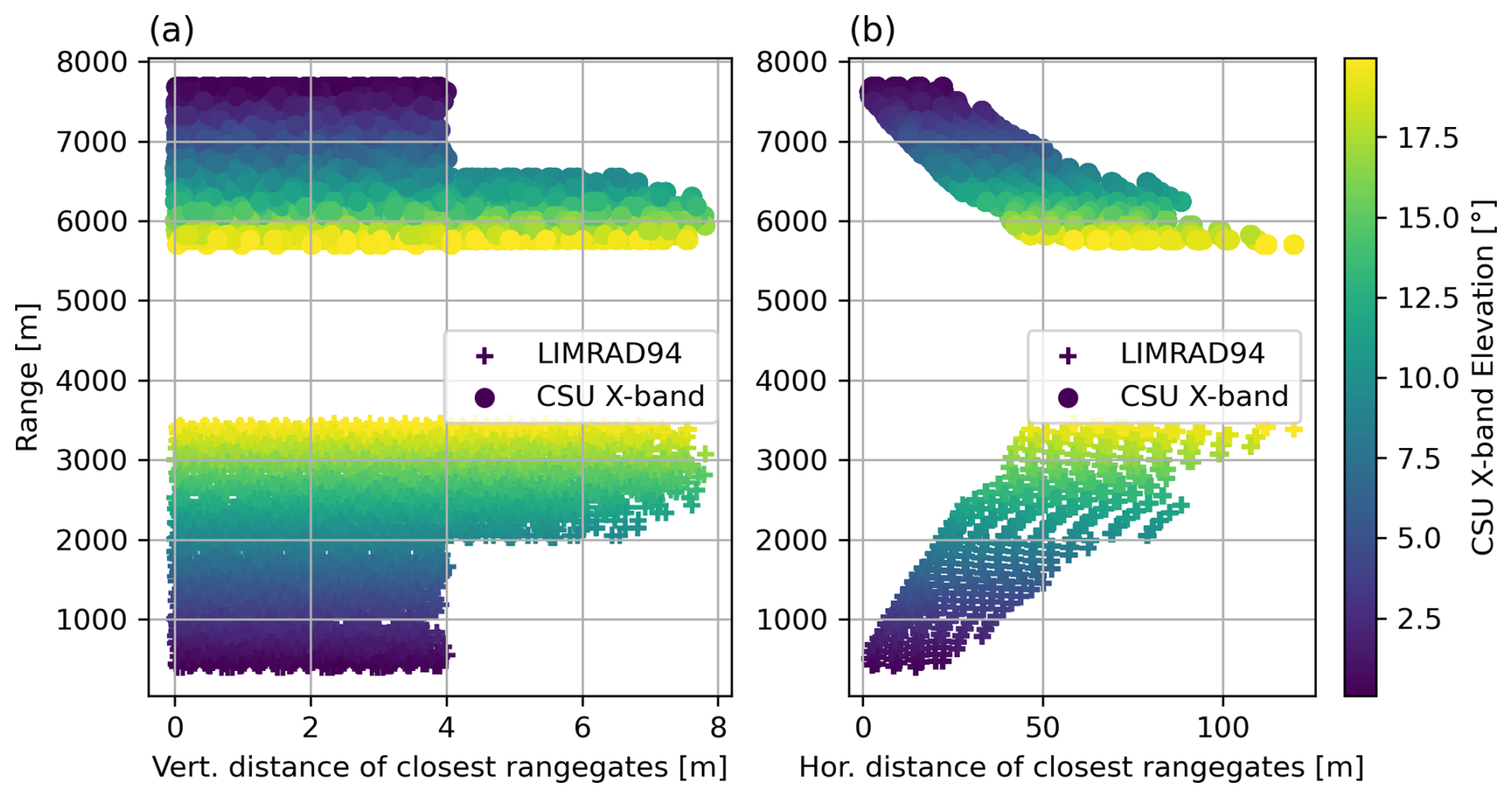
Figure B2Vertical (a) and horizontal distances (b) of the closest radar beams from LIMRAD94 and the CSU X-band during the RHI scans of the CSU X-band plotted against the respective radar range. The colors indicate the respective elevation angle of the CSU X-band.
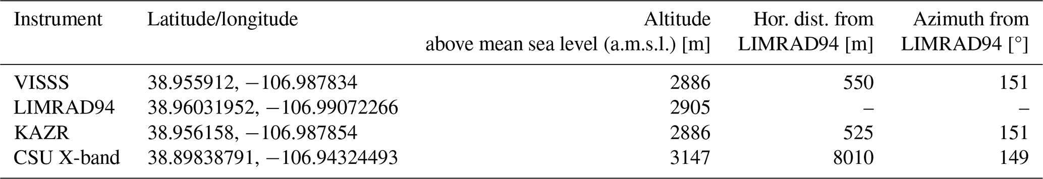
The SAIL data were obtained from the Atmospheric Radiation Measurement (ARM) user facility, a U.S. Department of Energy (DOE) Office of Science user facility managed by the Biological and Environmental Research Program LIMRAD94 (Kalesse-Los et al., 2023, https://doi.org/10.5439/2229846), VISSS (Maahn et al., 2024, https://doi.org/10.5439/2278627), the meteorological in situ 415 data of AMF2 (Kyrouac et al., 2021, https://doi.org/10.5439/1786358), the microwave radiometer retrieval products (Zhang, 1996, https://doi.org/10.5439/1027369), the ARM KAZR (Lindenmaier et al., 2023, https://doi.org/10.5439/1498936), and the CSU X-band (Chandrasekar, 2023, https://doi.org/10.5439/1888379). The ARM interpolated sonde product can be found in Jensen et al. (1998) (https://doi.org/10.5439/1095316).
AK collected and processed the LIMRAD94 data from CORSIPP, analyzed and plotted the data, and wrote the manuscript with contributions from all of the co-authors. LT and DO provided the DDA simulations. LT wrote Sect. 2.4.2. AM provided the T-matrix simulations and wrote Sect. 2.4.1. VE created Fig. 6 and wrote the caption. TV processed the EDR data. MM processed the VISSS data. HKL and MM acquired funding and guided the research project. AK, AM, MM, VE, AR, PB, LT, DO, and HKL participated in joint meetings to discuss the interpretation of polarimetric variables observed during the presented case study. All of the authors reviewed and edited the manuscript. The AI tool Writefull was used to correct spelling and typesetting.
The contact author has declared that none of the authors has any competing interests.
Publisher’s note: Copernicus Publications remains neutral with regard to jurisdictional claims made in the text, published maps, institutional affiliations, or any other geographical representation in this paper. While Copernicus Publications makes every effort to include appropriate place names, the final responsibility lies with the authors. Also, please note that this paper has not received English language copy-editing. Views expressed in the text are those of the authors and do not necessarily reflect the views of the publisher.
This article is part of the special issue “Fusion of radar polarimetry and numerical atmospheric modelling towards an improved understanding of cloud and precipitation processes (ACP/AMT/GMD inter-journal SI)”. It is not associated with a conference.
This research is funded by the Deutsche Forschungsgemeinschaft (DFG, German Research Foundation) – Project number: 408008112 (Characterization of orography-influenced riming and secondary ice production and their effects on precipitation rates using radar polarimetry and Doppler spectra – CORSIPP) within the Priority Program SPP 2115 “Polarimetric Radar Observations meet Atmospheric Modelling (PROM) – Fusion of Radar Polarimetry and Numerical Atmospheric Modelling Towards an Improved Understanding of Cloud and Precipitation Processes”. Contributions by L. von Terzi have been supported by the DFG Priority Program SPP2115 “Fusion of Radar Polarimetry and Numerical Atmospheric Modelling Towards an Improved Understanding of Cloud and Precipitation Processes” (PROM) under grant PROM-FRAGILE (project number 492234709). This research was supported by the Atmospheric Radiation Measurement (ARM) user facility, a U.S. Department of Energy (DOE) Office of Science user facility managed by the Biological and Environmental Research Program. This work was supported in part by the European Space Agency under the activity WInd VElocity Radar Nephoscope (WIVERN) Phase A Science and Requirements Consolidation Study, ESA Contract Number 4000144120/24/NL/IB/ab. We would like to thank the Rocky Mountain Biological Laboratory staff as well as ARM technicians for logistical and on-site technical support. We would like to thank Dr. Stefan Kneifel for his valuable feedback during our meetings discussing the paper material. We would also like to thank the PI of the CSU X-band radar Dr. V Chandrasekar and his team for providing access to the CSU X-band data set via the ARM data portal.
This research has been supported by the Deutsche Forschungsgemeinschaft (grant nos. 408008112 and 492234709) and the European Space Agency (grant no. 4000144120/24/NL/IB/ab). The publication of this article was funded by the Open Access Publishing Fund of Leipzig University and supported by the German Research Foundation within the Open Access Publication Funding program.
This paper was edited by Matthew Lebsock and reviewed by two anonymous referees.
Andrić, J., Kumjian, M. R., Zrnić, D. S., Straka, J. M., and Melnikov, V. M.: Polarimetric signatures above the melting layer in winter storms: An observational and modeling study, Journal of Applied Meteorology and Climatology, 52, 682–700, 2013. a, b, c, d, e, f
Bailey, M. P. and Hallett, J.: A comprehensive habit diagram for atmospheric ice crystals: Confirmation from the laboratory, AIRS II, and other field studies, Journal of the Atmospheric Sciences, 66, 2888–2899, 2009. a
Balakrishnan, N. and Zrnic, D. S.: Use of polarization to characterize precipitation and discriminate large hail, Journal of the Atmospheric Sciences, 47, 1525–1540, 1990. a
Battaglia, A., Martire, P., Caubet, E., Phalippou, L., Stesina, F., Kollias, P., and Illingworth, A.: End to end simulator for the WIVERN W-band Doppler conically scanning spaceborne radar, Atmospheric Measurement Techniques, 2021, 1–31, https://doi.org/10.5194/amt-2021-342, 2022. a
Bergeron, T.: On the physics of clouds and precipitation, Proc. 5th Assembly UGGI, Lisbon, Portugal, 1935, pp. 156–180, https://cir.nii.ac.jp/crid/1573105975504427392 (last access: 5 December 2024), 1935. a
Bringi, V. N., Keenan, T. D., and Chandrasekar, V.: Correcting C-band radar reflectivity and differential reflectivity data for rain attenuation: A self-consistent method with constraints, IEEE transactions on geoscience and remote sensing, 39, 1906–1915, 2001. a
Chandrasekar, V.: X-Band Precipitation Radar (XPRECIPRADAR), Atmospheric Radiation Measurement (ARM) Archive, Oak Ridge National Laboratory [data set], https://doi.org/10.5439/1888379, 2023.
Chellini, G. and Kneifel, S.: Turbulence as a Key Driver of Ice Aggregation and Riming in Arctic Low‐Level Mixed‐Phase Clouds, Revealed by Long‐Term Cloud Radar Observations, Geophysical Research Letters, 51, e2023GL106599, https://doi.org/10.1029/2023GL106599, 2024. a, b, c
Dedekind, Z., Grazioli, J., Austin, P. H., and Lohmann, U.: Heavy snowfall event over the Swiss Alps: did wind shear impact secondary ice production?, Atmos. Chem. Phys., 23, 2345–2364, https://doi.org/10.5194/acp-23-2345-2023, 2023. a, b, c
Dias Neto, J., Kneifel, S., Ori, D., Trömel, S., Handwerker, J., Bohn, B., Hermes, N., Mühlbauer, K., Lenefer, M., and Simmer, C.: The TRIple-frequency and Polarimetric radar Experiment for improving process observations of winter precipitation, Earth Syst. Sci. Data, 11, 845–863, https://doi.org/10.5194/essd-11-845-2019, 2019. a
Dunnavan, E. L., Carlin, J. T., Hu, J., Bukovčić, P., Ryzhkov, A. V., McFarquhar, G. M., Finlon, J. A., Matrosov, S. Y., and Delene, D. J.: Radar Retrieval Evaluation and Investigation of Dendritic Growth Layer Polarimetric Signatures in a Winter Storm, Journal of Applied Meteorology and Climatology, https://doi.org/10.1175/JAMC-D-21-0220.1, 2022. a
Erfani, E. and Mitchell, D. L.: Growth of ice particle mass and projected area during riming, Atmos. Chem. Phys., 17, 1241–1257, https://doi.org/10.5194/acp-17-1241-2017, 2017. a, b
Fairless, T., Jensen, M., Zhou, A., and Giangrande, S. E.: Interpolated sonde and gridded sonde value-added products, United States Department of Energy: Washington, DC, USA, https://doi.org/10.2172/1248938, 2021. a
Feldman, D. R., Aiken, A. C., Boos, W. R., Carroll, R. W. H., Chandrasekar, V., Collis, S., Creamean, J. M., De Boer, G., Deems, J., and DeMott, P. J.: The Surface Atmosphere Integrated Field Laboratory (SAIL) Campaign, Bulletin of the American Meteorological Society, 104, E2192–E2222, 2023. a, b
Foken, T. and Mauder, M.: Micrometeorology, Springer Atmospheric Sciences, Springer International Publishing, Cham, ISBN 978-3-031-47525-2 978-3-031-47526-9, https://doi.org/10.1007/978-3-031-47526-9, 2024. a
Grazioli, J., Lloyd, G., Panziera, L., Hoyle, C. R., Connolly, P. J., Henneberger, J., and Berne, A.: Polarimetric radar and in situ observations of riming and snowfall microphysics during CLACE 2014, Atmos. Chem. Phys., 15, 13787–13802, https://doi.org/10.5194/acp-15-13787-2015, 2015. a, b, c, d, e, f, g, h, i
Griffin, E. M., Schuur, T. J., and Ryzhkov, A. V.: A polarimetric analysis of ice microphysical processes in snow, using quasi-vertical profiles, Journal of Applied Meteorology and Climatology, 57, 31–50, 2018. a, b, c, d, e, f, g, h, i, j, k
Grzegorczyk, P., Yadav, S., Zanger, F., Theis, A., Mitra, S. K., Borrmann, S., and Szakáll, M.: Fragmentation of ice particles: laboratory experiments on graupel–graupel and graupel–snowflake collisions, Atmos. Chem. Phys., 23, 13505–13521, https://doi.org/10.5194/acp-23-13505-2023, 2023. a, b
Heflin, S., Abel, M., Biswas, S., Morales, A., Cifelli, R., Sedlar, J., Feldman, D., Chandrasekar, V., and Kennedy, P.: X-Band Radar and Surface-Based Observations of Cold-Season Precipitation in Western Colorado’s Complex Terrain, Journal of Hydrometeorology, https://doi.org/10.1175/JHM-D-23-0147.1, 2024. a
Heistermann, M., Jacobi, S., and Pfaff, T.: Technical Note: An open source library for processing weather radar data (wradlib), Hydrol. Earth Syst. Sci., 17, 863–871, https://doi.org/10.5194/hess-17-863-2013, 2013. a
Heymsfield, A. J., Schmitt, C., Bansemer, A., Gettelman, A., Field, P. R., and Liu, C.: Contributions of the liquid and ice phases to global surface precipitation: Observations and global climate modeling, Journal of the Atmospheric Sciences, 77, 2629–2648, 2020. a
Hogan, R. J., Field, P. R., Illingworth, A. J., Cotton, R. J., and Choularton, T. W.: Properties of embedded convection in warm-frontal mixed-phase cloud from aircraft and polarimetric radar, Quarterly Journal of the Royal Meteorological Society, 128, 451–476, https://doi.org/10.1256/003590002321042054, 2002. a, b, c, d
Hoose, C. and Möhler, O.: Heterogeneous ice nucleation on atmospheric aerosols: a review of results from laboratory experiments, Atmos. Chem. Phys., 12, 9817–9854, https://doi.org/10.5194/acp-12-9817-2012, 2012. a
Hu, J., Ryzhkov, A., and Dunnavan, E. L.: Vertical Profile Climatology of Polarimetric Radar Variables and Retrieved Microphysical Parameters in Synoptic and Lake Effect Snowstorms, Journal of Geophysical Research: Atmospheres, 129, e2024JD041318, https://doi.org/10.1029/2024JD041318, 2024. a
Hubbert, J. and Bringi, V.: Utilization of the radar polarimetric covariance matrix for polarization error and precipitation canting angle estimation, in: IGARSS 2003, 2003 IEEE International Geoscience and Remote Sensing Symposium. Proceedings (IEEE Cat. No.03CH37477), 7, 4456–4458 vol.7, https://doi.org/10.1109/IGARSS.2003.1295545, 2003. a
Illingworth, A. J., Battaglia, A., Bradford, J., Forsythe, M., Joe, P., Kollias, P., Lean, K., Lori, M., Mahfouf, J.-F., and Melo, S.: WIVERN: A new satellite concept to provide global in-cloud winds, precipitation, and cloud properties, Bulletin of the American Meteorological Society, 99, 1669–1687, 2018. a
Jensen, M., Giangrande, S., Fairless, T., and Zhou, A.: ARM Instrument: Interpolated Sonde, Atmospheric Radiation Measurement (ARM) Archive, Oak Ridge National Laboratory (ORNL) [data set], https://doi.org/10.5439/1095316, 1998. a
Kalesse, H., Szyrmer, W., Kneifel, S., Kollias, P., and Luke, E.: Fingerprints of a riming event on cloud radar Doppler spectra: observations and modeling, Atmos. Chem. Phys., 16, 2997–3012, https://doi.org/10.5194/acp-16-2997-2016, 2016. a
Kalesse-Los, H., Maahn, M., Ettrichratz, V., and Kotsche, A.: Characterization of Orography-Influenced Riming and Secondary Ice Production and Their Effects on Precipitation Rates Using Radar Polarimetry and Doppler Spectra (CORSIPP-SAIL), Tech. rep., Oak Ridge National Laboratory (ORNL), Oak Ridge, TN (United States) [data set], https://doi.org/10.5439/2229846, 2023. a, b
Kanji, Z. A., Ladino, L. A., Wex, H., Boose, Y., Burkert-Kohn, M., Cziczo, D. J., and Krämer, M.: Overview of ice nucleating particles, Meteorological Monographs, 58, 1–1, 2017. a
Kneifel, S., von Lerber, A., Tiira, J., Moisseev, D., Kollias, P., and Leinonen, J.: Observed relations between snowfall microphysics and triple-frequency radar measurements, Journal of Geophysical Research: Atmospheres, 120, 6034–6055, https://doi.org/10.1002/2015JD023156, 2015. a
Korolev, A. and Leisner, T.: Review of experimental studies of secondary ice production, Atmos. Chem. Phys., 20, 11767–11797, https://doi.org/10.5194/acp-20-11767-2020, 2020. a
Küchler, N., Kneifel, S., Löhnert, U., Kollias, P., Czekala, H., and Rose, T.: A W-Band Radar–Radiometer System for Accurate and Continuous Monitoring of Clouds and Precipitation, Journal of Atmospheric and Oceanic Technology, https://doi.org/10.1175/JTECH-D-17-0019.1, 2017. a
Kumjian, M. R.: Principles and Applications of Dual-Polarization Weather Radar. Part I: Description of the Polarimetric Radar Variables, Journal of Operational Meteorology, 1, https://doi.org/10.15191/nwajom.2013.0119, 2013. a
Kyrouac, J., Shi, Y., and Tuftedal, M.: ARM-standard Meteorological Instrumentation at Surface, Atmospheric Radiation Measurement (ARM) Archive, Oak Ridge National Laboratory (ORNL) [data set], https://doi.org/10.5439/1786358, 2021. a
Leinonen, J., Kneifel, S., Moisseev, D., Tyynelä, J., Tanelli, S., and Nousiainen, T.: Evidence of nonspheroidal behavior in millimeter‐wavelength radar observations of snowfall, Journal of Geophysical Research: Atmospheres, 117, 2012JD017680, https://doi.org/10.1029/2012JD017680, 2012. a
Liao, L., Meneghini, R., Tian, L., and Heymsfield, G. M.: Retrieval of snow and rain from combined X-and W-band airborne radar measurements, IEEE transactions on geoscience and remote sensing, 46, 1514–1524, 2008. a
Lindenmaier, I., Johnson, K., Matthews, A., Wendler, T., Melo de Castro, V., Deng, M., Rocque, M., and Feng, Y.-C.: Ka ARM Zenith Radar (KAZRCFRGE), 2022-11-10 to 2023-06-06, ARM Mobile Facility (GUC), Gunnison, CO; AMF2 (main site for SAIL) (M1), Atmospheric Radiation Measurement (ARM) Archive [data set], https://doi.org/10.5439/1498936, 2023. a
Lu, Y., Aydin, K., Clothiaux, E. E., and Verlinde, J.: Retrieving cloud ice water content using millimeter-and centimeter-wavelength radar polarimetric observables, Journal of Applied Meteorology and Climatology, 54, 596–604, 2015. a, b
Luke, E. P., Yang, F., Kollias, P., Vogelmann, A. M., and Maahn, M.: New insights into ice multiplication using remote-sensing observations of slightly supercooled mixed-phase clouds in the Arctic, Proceedings of the National Academy of Sciences, 118, e2021387118, https://doi.org/10.1073/pnas.2021387118, 2021. a
Maahn, M., Löhnert, U., Kollias, P., Jackson, R. C., and McFarquhar, G. M.: Developing and Evaluating Ice Cloud Parameterizations for Forward Modeling of Radar Moments Using in situ Aircraft Observations, Journal of Atmospheric and Oceanic Technology, https://doi.org/10.1175/JTECH-D-14-00112.1, 2015. a, b
Maahn, M., Ettrichrätz, V., and Steinke, I.: VISSS Raw data from SAIL at Gothic from November 2022 to June 2023, Atmospheric Radiation Measurement (ARM) Archive, Oak Ridge National Laboratory (ORNL), [data set], https://doi.org/10.5439/2278627, 2024. a
Maahn, M., Moisseev, D., Steinke, I., Maherndl, N., and Shupe, M. D.: Introducing the Video In Situ Snowfall Sensor (VISSS), Atmos. Meas. Tech., 17, 899–919, https://doi.org/10.5194/amt-17-899-2024, 2024. a, b, c, d, e, f
Majewski, A., French, J. R., and Haimov, S.: Airborne Radar Doppler Spectrum Width as a Scale-Dependent Turbulence Metric, Journal of Atmospheric and Oceanic Technology, https://doi.org/10.1175/JTECH-D-23-0056.1, 2023. a
Marshall, J. S.: Precipitation trajectories and patterns, Journal of Atmospheric Sciences, 10, 25–29, 1953. a
Mishchenko, M. I.: Calculation of the amplitude matrix for a nonspherical particle in a fixed orientation, Applied Optics, 39, 1026–1031, https://doi.org/10.1364/AO.39.001026, 2000. a
Moisseev, D. N., Lautaportti, S., Tyynela, J., and Lim, S.: Dual‐polarization radar signatures in snowstorms: Role of snowflake aggregation, Journal of Geophysical Research: Atmospheres, 120, 12644–12655, https://doi.org/10.1002/2015JD023884, 2015. a, b, c, d, e
Myagkov, A., Seifert, P., Bauer-Pfundstein, M., and Wandinger, U.: Cloud radar with hybrid mode towards estimation of shape and orientation of ice crystals, Atmos. Meas. Tech., 9, 469–489, https://doi.org/10.5194/amt-9-469-2016, 2016a. a
Myagkov, A., Seifert, P., Wandinger, U., Bühl, J., and Engelmann, R.: Relationship between temperature and apparent shape of pristine ice crystals derived from polarimetric cloud radar observations during the ACCEPT campaign, Atmos. Meas. Tech., 9, 3739–3754, https://doi.org/10.5194/amt-9-3739-2016, 2016b. a, b
Myagkov, A., Kneifel, S., and Rose, T.: Evaluation of the reflectivity calibration of W-band radars based on observations in rain, Atmos. Meas. Tech., 13, 5799–5825, https://doi.org/10.5194/amt-13-5799-2020, 2020. a
Oguchi, T.: Electromagnetic wave propagation and scattering in rain and other hydrometeors, Proceedings of the IEEE, 71, 1029–1078, https://doi.org/10.1109/PROC.1983.12724, 1983. a
Ori, D., von Terzi, L., Karrer, M., and Kneifel, S.: snowScatt 1.0: consistent model of microphysical and scattering properties of rimed and unrimed snowflakes based on the self-similar Rayleigh–Gans approximation, Geosci. Model Dev., 14, 1511–1531, https://doi.org/10.5194/gmd-14-1511-2021, 2021. a, b, c
Oue, M., Kollias, P., Ryzhkov, A., and Luke, E. P.: Toward Exploring the Synergy Between Cloud Radar Polarimetry and Doppler Spectral Analysis in Deep Cold Precipitating Systems in the Arctic, Journal of Geophysical Research: Atmospheres, 123, 2797–2815, https://doi.org/10.1002/2017JD027717, 2018.. a, b
Pfitzenmaier, L., Dufournet, Y., Unal, C. M., and Russchenberg, H. W.: Retrieving fall streaks within cloud systems using Doppler radar, Journal of Atmospheric and Oceanic Technology, 34, 905–920, 2017. a
Ramelli, F., Henneberger, J., David, R. O., Lauber, A., Pasquier, J. T., Wieder, J., Bühl, J., Seifert, P., Engelmann, R., Hervo, M., and Lohmann, U.: Influence of low-level blocking and turbulence on the microphysics of a mixed-phase cloud in an inner-Alpine valley, Atmos. Chem. Phys., 21, 5151–5172, https://doi.org/10.5194/acp-21-5151-2021, 2021. a, b, c, d, e, f
Ryzhkov, A., Pinsky, M., Pokrovsky, A., and Khain, A.: Polarimetric Radar Observation Operator for a Cloud Model with Spectral Microphysics, Journal of Applied Meteorology and Climatology, https://doi.org/10.1175/2010JAMC2363.1, 2011. a
Ryzhkov, A. V. and Zrnic, D. S.: Radar Polarimetry for Weather Observations, Springer Atmospheric Sciences, Springer International Publishing, Cham, ISBN 978-3-030-05092-4, 978-3-030-05093-1, https://doi.org/10.1007/978-3-030-05093-1, 2019. a, b, c, d
Ryzhkov, A. V., Zrnic, D. S., Hubbert, J. C., Bringi, V. N., Vivekanandan, J., and Brandes, E. A.: Polarimetric radar observations and interpretation of co-cross-polarcorrelation coefficients, Journal of Atmospheric and Oceanic Technology, 19, 340–354, 2002. a, b
Sanz, E., Vega, C., Espinosa, J. R., Caballero-Bernal, R., Abascal, J. L. F., and Valeriani, C.: Homogeneous Ice Nucleation at Moderate Supercooling from Molecular Simulation, Journal of the American Chemical Society, 135, 15008–15017, https://doi.org/10.1021/ja4028814, 2013. a
Schrom, R. S. and Kumjian, M. R.: Connecting microphysical processes in Colorado winter storms with vertical profiles of radar observations, Journal of Applied Meteorology and Climatology, 55, 1771–1787, 2016. a, b, c
Schrom, R. S. and Kumjian, M. R.: Bulk-Density Representations of Branched Planar Ice Crystals: Errors in the Polarimetric Radar Variables, Journal of Applied Meteorology and Climatology, https://doi.org/10.1175/JAMC-D-17-0114.1, 2018. a
Sheridan, L. M., Harrington, J. Y., Lamb, D., and Sulia, K.: Influence of ice crystal aspect ratio on the evolution of ice size spectra during vapor depositional growth, Journal of the atmospheric sciences, 66, 3732–3743, 2009. a
Takahashi, T.: Influence of liquid water content and temperature on the form and growth of branched planar snow crystals in a cloud, Journal of the Atmospheric Sciences, 71, 4127–4142, 2014. a, b
Trömel, S., Kumjian, M. R., Ryzhkov, A. V., Simmer, C., and Diederich, M.: Backscatter Differential Phase—Estimation and Variability, Journal of Applied Meteorology and Climatology, https://doi.org/10.1175/JAMC-D-13-0124.1, 2013. a, b, c, d
Trömel, S., Ryzhkov, A. V., Hickman, B., Mühlbauer, K., and Simmer, C.: Polarimetric Radar Variables in the Layers of Melting and Dendritic Growth at X Band—Implications for a Nowcasting Strategy in Stratiform Rain, Journal of Applied Meteorology and Climatology, https://doi.org/10.1175/JAMC-D-19-0056.1, 2019. a
Trömel, S., Simmer, C., Blahak, U., Blanke, A., Doktorowski, S., Ewald, F., Frech, M., Gergely, M., Hagen, M., Janjic, T., Kalesse-Los, H., Kneifel, S., Knote, C., Mendrok, J., Moser, M., Köcher, G., Mühlbauer, K., Myagkov, A., Pejcic, V., Seifert, P., Shrestha, P., Teisseire, A., von Terzi, L., Tetoni, E., Vogl, T., Voigt, C., Zeng, Y., Zinner, T., and Quaas, J.: Overview: Fusion of radar polarimetry and numerical atmospheric modelling towards an improved understanding of cloud and precipitation processes, Atmos. Chem. Phys., 21, 17291–17314, https://doi.org/10.5194/acp-21-17291-2021, 2021. a
Vogl, T., Maahn, M., Kneifel, S., Schimmel, W., Moisseev, D., and Kalesse-Los, H.: Using artificial neural networks to predict riming from Doppler cloud radar observations, Atmos. Meas. Tech., 15, 365–381, https://doi.org/10.5194/amt-15-365-2022, 2022. a
Vogl, T., Radenz, M., Ramelli, F., Gierens, R., and Kalesse-Los, H.: PEAKO and peakTree: tools for detecting and interpreting peaks in cloud radar Doppler spectra – capabilities and limitations, Atmos. Meas. Tech., 17, 6547–6568, https://doi.org/10.5194/amt-17-6547-2024, 2024. a
von Terzi, L., Dias Neto, J., Ori, D., Myagkov, A., and Kneifel, S.: Ice microphysical processes in the dendritic growth layer: a statistical analysis combining multi-frequency and polarimetric Doppler cloud radar observations, Atmos. Chem. Phys., 22, 11795–11821, https://doi.org/10.5194/acp-22-11795-2022, 2022. a, b, c, d, e, f, g, h, i, j
Wegener, A.: Thermodynamik der atmosphäre, JA Barth, ISBN 978-3836429658, 1911. a
Wendisch, M., Crewell, S., Ehrlich, A., Herber, A., Kirbus, B., Lüpkes, C., Mech, M., Abel, S. J., Akansu, E. F., Ament, F., Aubry, C., Becker, S., Borrmann, S., Bozem, H., Brückner, M., Clemen, H.-C., Dahlke, S., Dekoutsidis, G., Delanoë, J., De La Torre Castro, E., Dorff, H., Dupuy, R., Eppers, O., Ewald, F., George, G., Gorodetskaya, I. V., Grawe, S., Groß, S., Hartmann, J., Henning, S., Hirsch, L., Jäkel, E., Joppe, P., Jourdan, O., Jurányi, Z., Karalis, M., Kellermann, M., Klingebiel, M., Lonardi, M., Lucke, J., Luebke, A. E., Maahn, M., Maherndl, N., Maturilli, M., Mayer, B., Mayer, J., Mertes, S., Michaelis, J., Michalkov, M., Mioche, G., Moser, M., Müller, H., Neggers, R., Ori, D., Paul, D., Paulus, F. M., Pilz, C., Pithan, F., Pöhlker, M., Pörtge, V., Ringel, M., Risse, N., Roberts, G. C., Rosenburg, S., Röttenbacher, J., Rückert, J., Schäfer, M., Schaefer, J., Schemann, V., Schirmacher, I., Schmidt, J., Schmidt, S., Schneider, J., Schnitt, S., Schwarz, A., Siebert, H., Sodemann, H., Sperzel, T., Spreen, G., Stevens, B., Stratmann, F., Svensson, G., Tatzelt, C., Tuch, T., Vihma, T., Voigt, C., Volkmer, L., Walbröl, A., Weber, A., Wehner, B., Wetzel, B., Wirth, M., and Zinner, T.: Overview: quasi-Lagrangian observations of Arctic air mass transformations – introduction and initial results of the HALO–(𝒜𝒞)3 aircraft campaign, Atmos. Chem. Phys., 24, 8865–8892, https://doi.org/10.5194/acp-24-8865-2024, 2024. a
Widener, K., Bharadwaj, N., and Johnson, K.: Ka-Band ARM Zenith Radar (KAZR) Instrument Handbook, Tech. Rep. DOE/SC-ARM/TR-106, PNNL; Richland, WA, https://doi.org/10.2172/1035855, 2012. a, b
Yurkin, M. A. and Hoekstra, A. G.: The discrete-dipole-approximation code ADDA: Capabilities and known limitations, Journal of Quantitative Spectroscopy and Radiative Transfer, 112, 2234–2247, https://doi.org/10.1016/j.jqsrt.2011.01.031, 2011. a
Zhang, D.: ARM Instrument: MWR Retrievals, Atmospheric Radiation Measurement (ARM) Archive, Oak Ridge National Laboratory (ORNL) [data set], https://doi.org/10.5439/1027369, 1996. a
- Abstract
- Introduction
- Data and methods
- Results and discussion
- Summary and conclusions
- Appendix A: Chirp tables of the polarimetric W-band radar
- Appendix B: Evaluation of antenna pointing and measurement comparability
- Code and data availability
- Author contributions
- Competing interests
- Disclaimer
- Special issue statement
- Acknowledgements
- Financial support
- Review statement
- References