Aerosol effective radius governs the relationship between cloud condensation nuclei (CCN) concentration and aerosol backscatter

Understanding the vertical distribution of cloud condensation nuclei (CCN) concentrations is crucial for reducing uncertainty associated with aerosol–cloud interactions (ACIs) and their effective radiative forcing. Many studies take advantage of widely available remote sensing observations to develop proxies, parameterizations, and relationships between CCN concentration and aerosol optical properties (AOPs). Such methods generally provide a good constraint for CCN concentration, but many uncertainties and limitations exist, generally related to high relative humidity (RH), environments with internal or external mixtures of several different aerosol types, and differences in parts of the aerosol size distribution relevant to both CCN and AOPs. In this study, we use in situ observations of the aerosol size distribution and chemical composition in a recent airborne field campaign to inform theoretical calculations of CCN concentration (CCN_theory) and aerosol backscatter at 532 nm (BSC_theory) with the purpose of understanding the dominant governing factors of the CCN_theory–BSC_theory relationship. Estimates from random forest models indicate that, for smoke, marine, and urban aerosols, the aerosol size distribution, as parameterized by the effective radius (R_eff), is the most important predictor of the CCN_theory–BSC_theory relationship. We further investigate how R_eff impacts CCN_theory : BSC_theory and find an exponential relationship between the parameters. We find that modeling CCN_theory : BSC_theory using this exponential R_eff relationship can explain about 68 %–79 % of the variance in the CCN_theory–BSC_theory relationship. These findings suggest that including information about aerosol size is critical for future studies in constraining CCN concentration from AOPs.

1 Introduction

Natural and anthropogenic atmospheric aerosols and their interactions with clouds and radiation have a significant role in climate change and uncertainties in future climate predictions. Specifically, the highest uncertainties compared to other climate forcings are attributed to effective radiative forcing due to interactions between aerosols and clouds (ERF_aci; Forster et al., 2021). Much of the uncertainty in aerosol–cloud interactions (ACIs) is due to limited process-level understanding (Boucher et al., 2013) and observing methods. For example, there is limited ability for passive satellite instruments to retrieve cloud and aerosol properties simultaneously in the same environment. Hygroscopic aerosol growth in high-relative-humidity (RH) environments can also complicate observations (Rosenfeld et al., 2014). Additionally, varying observational scales and meteorological conditions may buffer the responses of clouds to aerosol perturbations (Stevens and Feingold, 2009).

Untangling the impact of ACIs from such observational complications requires information on the distribution of those aerosols that interact with clouds by nucleating cloud droplets, i.e., cloud condensation nuclei (CCN). More specifically, knowledge of the vertical distribution of CCN concentration relative to clouds is needed to properly assess and understand ACIs. The main challenge in understanding the vertical distribution of CCN lies in the sparsity of in situ observations. Ground-based observations are useful in terms of the length of available observations, but they lack vertical extent. Alternatively, aircraft-based observations can provide observations of CCN closer to the cloud base over shorter campaign periods, but these observations are expensive and less frequently available. Therefore, many studies have developed parameterizations, proxies, and retrieval methods to determine CCN from more commonly available remotely sensed observations of aerosol optical properties (AOPs).

One of the most widely used proxies for CCN concentration is aerosol optical depth (AOD), a column-integrated measure of aerosol extinction (EXT). While AOD may approximate CCN concentration over large spatiotemporal extents (Stier, 2016), it often cannot fully explain CCN variance (Andreae, 2009; Shinozuka et al., 2015; Stier, 2016; Choudhury and Tesche, 2022a; Choudhury and Tesche, 2022b), lacks any information about the vertical distribution of CCN, and is subject to effects of aerosol swelling and cloud contamination (Rosenfeld et al., 2016; Patel et al., 2024). Several studies have related CCN to a combination of other AOPs from lidar and satellite such as aerosol extinction, scattering and backscattering coefficients, backscatter fraction, which is the ratio of backscattering to total scattering, single-scattering albedo (SSA), scattering Ångström exponent, and aerosol index (AI), with the latter being the product of Ångström exponent and extinction (Ghan and Collins, 2004; Ghan et al., 2006; Kapustin et al., 2006; Shinozuka et al., 2009; Jefferson, 2010; Liu and Li, 2014; Shinozuka et al., 2015; Mamouri and Ansmann, 2016; Stier, 2016; Tskeri et al., 2017; Lv et al., 2018; Haarig et al., 2019; Shen et al., 2019; Choudhury and Tesche, 2022a; Choudhury and Tesche, 2022b; Lenhardt et al., 2023; Patel et al., 2024; Redemann and Gao, 2024). Among such approaches, AOPs can provide constraints for CCN, but several underlying uncertainties and limitations exist.

One fundamental issue in relating CCN concentration to AOPs is that particles that act as CCN are generally smaller than particles that have a more significant impact on AOPs when measured at visible wavelengths. Most CCN fall in the Aitken and accumulation modes of the aerosol size distribution, and studies have shown that changes in the aerosol size distribution are the primary drivers of changes in the CCN spectrum (Dusek et al., 2006; Miao et al., 2015; Perkins et al., 2022). In terms of AOPs, many are dominated by coarse-mode particles (Shinozuka et al., 2015), and optical measurements tend to be insensitive to small particles that activate as CCN (Jefferson, 2010), causing further uncertainty in correlating both measurements. Another common issue in relating CCN to AOPs is hygroscopic growth of aerosols at high ambient RH. Hygroscopic growth increases aerosol size, thus increasing their light scattering. However, the lack of a corresponding increase in CCN concentration (Shinozuka et al., 2015) causes CCN–AOP relationships to change rapidly at high RH (Liu and Li, 2014; Shinozuka et al., 2015; Stier, 2016; Wang et al., 2025). Since CCN are of particular interest in humid environments near the cloud base, this issue can become problematic for ACI applicability. Additionally, aerosol chemical composition influences both CCN concentration and AOPs and their relationship. Some studies have found that CCN–AOP relationships are more uncertain for observations of marine aerosols (Liu and Li, 2014; Shen et al., 2019; Choudhury et al., 2025), which may be related to their more dominant coarse mode and the tendency for marine aerosol shapes to be non-spherical (Fitzgerald, 1991; von Hoyningen-Huene and Posse, 1997; Bi et al., 2018). In summary, the three most common sources of potential error when relating CCN to AOPs are related to high ambient RH, the shape of the aerosol size distribution, and the aerosol chemical composition.

While each of these sources of uncertainty and potentially weak correlation have been noted by numerous studies, many that investigate underlying causes of error focus on each source individually. Additionally, many studies that take a modeling or calculation-based approach to investigating CCN and/or AOPs often use idealized, generated, or average size distributions as a starting point (Li et al., 2015; Lowe et al., 2016; Shen et al., 2019) or vary individual observed size distributions in terms of concentration but not the functional shape (Chuang et al., 2000). While this approach avoids the uncertainties inherent to in situ aerosol size distribution observations, it also does not capture the full range of variability seen in observed size distributions.

In this study, we investigate the collective impact of ambient RH, aerosol size distribution, and aerosol chemical composition on CCN–AOP relationships using a broad range of actual observed aerosol properties. Specifically, we follow and expand on Lenhardt et al. (2023), hereafter L23, by applying the same methodology to multiple aerosol types under a variety of ambient RH conditions observed during the Aerosol Cloud meTeorology Interactions oVer the western ATlantic Experiment (ACTIVATE) campaign (Sect. 2). L23 focused on optimizing a linear regression model between in situ CCN concentration and aerosol extinction and backscatter from the High Spectral Resolution Lidar 2 (HSRL-2) for observations of smoke in mostly dry (RH ≤ 50 %) conditions during the ObseRvations of Aerosols above CLouds and their intEractionS (ORACLES) campaign. In this study, we perform an L23-motivated analysis and follow it with a more in-depth investigation of the underlying factors that govern how CCN concentration and backscatter at 532 nm (BSC) are related to understand which one may be the most important predictor. To achieve this, we perform observation-informed theoretical calculations of CCN (CCN_theory) and aerosol BSC (BSC_theory) using in situ-observed aerosol size distributions and chemical compositions as inputs into both the κ–Köhler and Mie theories (Sects. 3 and 4). Throughout the study, all observations and calculations of BSC will be at 532 nm. Requisite input data for both calculations come from ACTIVATE in situ observations, meaning that we do not assume average values for the hygroscopicity parameter or use a singular idealized, representative aerosol size distribution. This approach allows us to capture the observation-informed variability in aerosol size and composition to investigate how such variability impacts the theoretical relationship between CCN and BSC.

2 Field deployment background and motivation for the present study

The National Aeronautics and Space Administration (NASA) ACTIVATE campaign took place between February 2020 and June 2022 across six deployments over the northwestern Atlantic Ocean and generated a unique in situ and remote sensing data set relevant for investigating aerosol–cloud–meteorology interactions. Unlike subtropical regions frequently chosen for ACI-related campaigns, the northwestern Atlantic features numerous cloud types, including warm and mixed-phase cumulus, that are less well-understood than stratocumulus cloud decks (Sorooshian et al., 2023). Additionally, observations over different seasons allow for the analysis of a wide range of aerosol and meteorological conditions. Data were collected using coordinated flights of the NASA Langley Research Center HU-25 Falcon for in situ measurements and King Air aircraft for remote sensing observations. In this study, we collocate in situ and remote sensing observations from both aircraft. The study region and the locations of these collocated data points, broken down by aerosol type, are shown in Fig. 1.

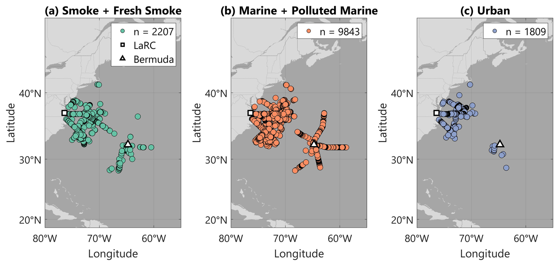
Figure 1 Maps showing the ACTIVATE study area and locations of collocated data points for observations of (a) smoke and fresh smoke, (b) marine and polluted marine, and (c) urban aerosols. Langley Research Center (LaRC) in Hampton, Virginia, and Bermuda, the two major bases of operations, are also shown.

During the ACTIVATE campaign, the HU-25 Falcon aircraft conducted profiling flights within, above, and below boundary layer clouds while collecting in situ observations, and the spatially coordinated King Air flew above the Falcon (∼ 9 km), conducting remote sensing observations and launching dropsondes (Sorooshian et al., 2023). Following the methodology of L23, our first step is a direct comparison between observed CCN concentration (CCN_obs) and BSC at 532 nm (BSC_obs), the instrumentation for which is described in Sect. 3.1. Due to the different spatiotemporal resolutions of the in situ and remote sensing data sets, we first collocate both data sets to enable a one-to-one comparison. Fortunately, ACTIVATE prioritized systematic and spatially coordinated flights between both aircraft, with approximately 73 % of the cumulative data set having the two aircraft within 6 km and 5 min of one another (Schlosser et al., 2024). Therefore, collocation between both aircraft results in many collocated data points for the remaining analyses. Our collocation process uses three independent collocation criteria to find in situ measurements that fall within a set amount of time (d$t=\pm \mathrm{0.1}$ h) from when an HSRL-2 profile was measured, within a set horizontal distance (d$d=\pm \mathrm{0.01}\mathit{°}$ or $\pm \sim$1.1 km) from the profile, and within set vertical bins (dh = 45 m). After these criteria have been applied, in situ observations that meet all three criteria are averaged to enable a one-to-one comparison with HSRL-2 BSC. For more details on our sensitivity testing method to determine appropriate values for dt, dd, and dh and for a schematic describing the collocation process, see L23.

We analyze the correlation between collocated CCN_obs and BSC_obs separated by aerosol type (Fig. 2), indicated by the HSRL-2 Aerosol ID product (Sect. 3.1.2). In this study, we combine smoke with fresh smoke (SFS) and marine with polluted marine (MPM) due to similarity in their optical properties. We also consider the urban or pollution (URB) aerosol type. Following L23, we fit all relationships using a bisector regression to account for both variables being measured with observational uncertainty. Additionally, we show the coefficient of determination (R²), a measure of the proportion of variation in CCN_obs that is explained by the variation in BSC_obs; the root mean square error (RMSE), a measure of the average difference between linear-regression-predicted CCN and CCN_obs; and the number of data points (n). Observations are limited to a small supersaturation range of 0.36 %–0.38 %, and marker colors correspond to ambient RH. One of our primary findings in L23 was that the correlation between CCN_obs and BSC_obs was strongest at low ambient RH (≤50 %). Therefore, we show separate statistics and regression lines for all observations and the subset observed at RH ≤ 50 %.

R² values for all aerosol types across the full RH spectrum range from 0.0014 to 0.14, and those for RH ≤ 50 % range from 0.0023 to 0.038, suggesting that there is no aerosol type for which variations in CCN_obs are well-explained by changes in BSC_obs. For all RH values, R² is strongest for URB, while smoke has the highest R² under limited-RH conditions. For SFS and URB, R² decreases when limiting the data set to low RH, contrary to the findings of L23. In the case of the SFS and MPM analyses, RMSE increases when limiting the data set to low RH. Overall, RMSE varies from 342 to 592 cm⁻³, and these values are significantly higher than the median CCN_obs uncertainty of approximately 150 cm⁻³ for this data set (assuming a relative uncertainty of 10 %, as reported in the data). Additionally, we see the impact of hygroscopic growth most clearly in the MPM results, where several observations made at RH > 80 % show increased BSC_obs associated with nearly constant and low CCN_obs values. This aerosol type is primarily influenced by sea salt, one of the most hygroscopic aerosols with a high growth factor and kappa that can range from 0.91 to 1.33 (Petters and Kreidenweis, 2007). If we consider, as an example, the subset of SFS CCN_obs with BSC_obs between 0.0006–0.0008 km⁻¹ sr⁻¹ and RH between 80 %–90 %, both small ranges that capture the peak of observed conditions for SFS aerosols, CCN_obs ranges from 25 to 2128 cm⁻³. While this range captures the maximum observed variability, similar magnitudes can also be seen for MPM and URB aerosols within similar small ranges of BSC_obs and RH.

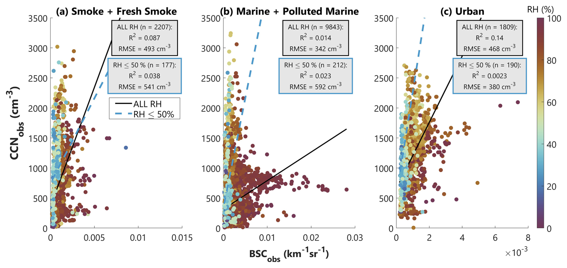
Figure 2 Bisector regression of CCN_obs vs. BSC_obs at 532 nm for (a) smoke and fresh smoke, (b) marine and polluted marine, and (c) urban aerosols. This combined data set covers all years of ACTIVATE and represents 76 flight days. Supersaturation for these observations ranges between 0.36 %–0.38 %. The number of collocated data points (n) is given, as well as the R² value and root mean square error (RMSE). Statistics are given for the full data set (black-outlined box), as well as the subset of data observed at RH ≤ 50 % (blue-outlined box). The solid black line of best fit applies to the full data set, and the dashed blue line of best fit applies to the low-RH subset of data.

Unlike in L23, the direct relationship between CCN_obs and BSC_obs in the ACTIVATE data cannot be represented well using a linear approximation. We find that, even when limiting the data set to observations made at low ambient RH, the correlation is weak, and scatter around the regression line is high. Additionally, we find that within individual aerosol types and for small ranges of BSC_obs and ambient RH, the magnitude of CCN_obs can vary by nearly 2 orders of magnitude. Another difference between this analysis and the ORACLES results is the relatively low frequency of observations made in low-RH environments. While more than half of the smoke plume observations in ORACLES were made at low RH, only about 2 %–10 % of the observations in Fig. 2 were observed at low RH since the HU-25 Falcon primarily sampled in the marine boundary layer (MBL) during ACTIVATE. This observed non-linearity between CCN_obs and BSC_obs in the ACTIVATE data (Fig. 2) serves as motivation for the rest of this study – unlike L23, we do not try to optimize a linear relationship between CCN_obs and BSC_obs. Rather, we perform calculations of CCN_theory and BSC_theory based on actual observations of aerosol size distribution and chemical composition to understand this observed non-linearity and to determine which factors dominate in governing the CCN_theory–BSC_theory relationship. The goal of this theoretical investigation is to use observations from ACTIVATE as a basis to determine what additional information is most important in constraining CCN concentration from remotely sensed AOPs such as lidar aerosol backscatter.

3 Data and theoretical calculation methods

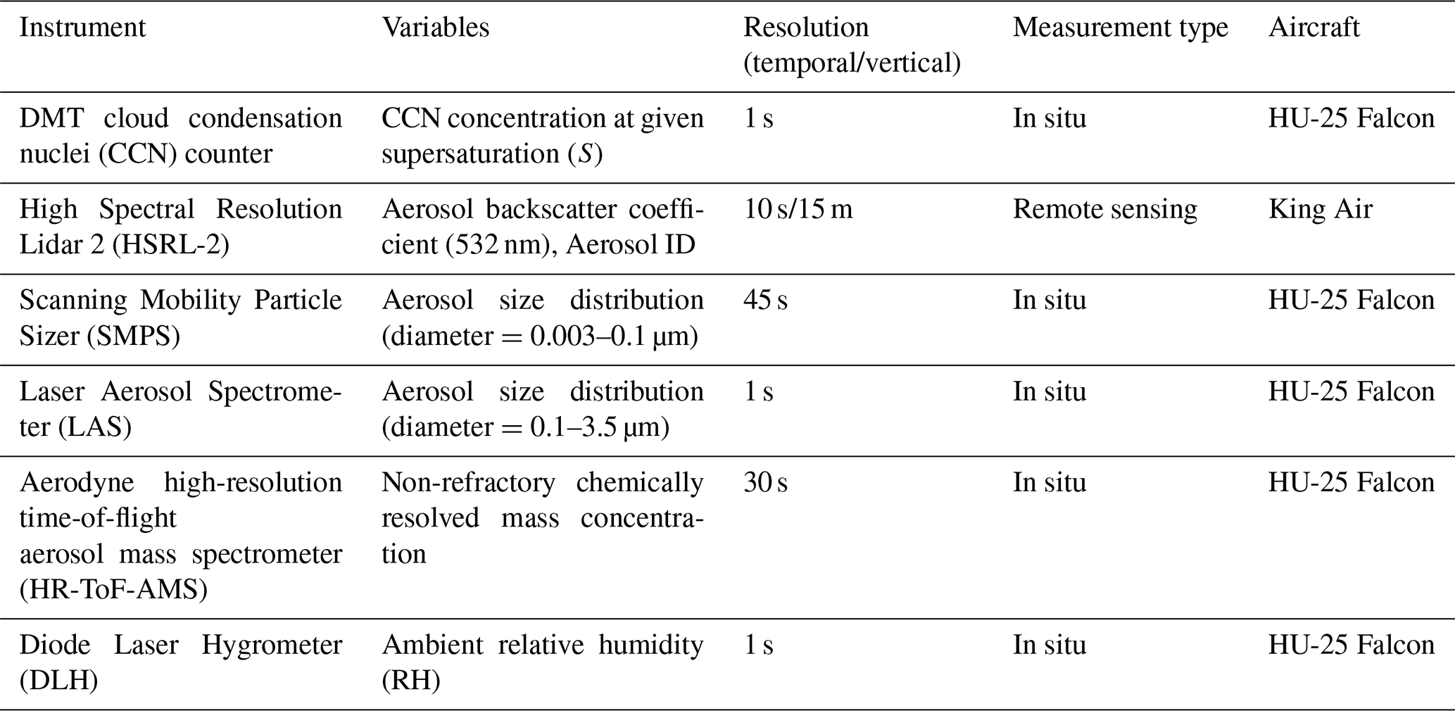
The four primary ACTIVATE data sets used in this study are described in Sect. 3.1 and summarized in Table 1. Our methodologies for the calculation of CCN_theory and BSC_theory are outlined in Sect. 3.2 and 3.3, respectively. Lastly, we describe pre-analysis data-filtering steps in Sect. 3.4.

3.1 Instrumentation

3.1.1 Droplet Measurement Technologies (DMT) CCN counter

The Droplet Measurement Technologies (DMT) CCN counter measures in situ CCN concentration at multiple levels of water vapor supersaturation (S) and can be run in constant S or scanning S modes (Moore and Nenes, 2009), with most observations from ACTIVATE being made at approximately S=0.37 %. This instrument is designed as a continuous-flow streamwise thermal-gradient chamber (CFSTGC; Roberts and Nenes, 2005), where a quasi-uniform supersaturation is generated in the center of a cylindrical flow chamber as heat and water vapor are continuously transported from wetted walls under a temperature gradient. Supersaturation levels vary based on the instrument pressure, flow rate, and imposed column temperature gradient. The continuous-flow feature enables quick (1 Hz frequency) sampling (Roberts and Nenes, 2005), which is important for airborne observations in quickly evolving environments. At the end of the growth chamber, aerosols that activated into droplets with a radius greater than 0.5 µm are counted as CCN. The uncertainty reported for CCN concentration is ±10 %, with a supersaturation uncertainty of ±0.04 % (Rose et al., 2008).

3.1.2 High Spectral Resolution Lidar 2 (HSRL-2)

The NASA Langley Research Center HSRL-2 measures aerosol backscatter and depolarization at 355, 532, and 1064 nm and aerosol extinction via the HSRL technique at 355 and 532 nm (Shipley et al., 1983; Hair et al., 2008; Burton et al., 2018). Using the spectral distribution of the return signal, the HSRL measurement technique enables separation of aerosol and molecular backscatter signals, which, in turn, allows for independent, accurate retrieval of aerosol backscatter and extinction profiles without reliance on external assumptions such as the value of the lidar ratio, as is common for basic elastic backscatter lidars (Hair et al., 2008). In this study, we focus on particulate backscatter at 532 nm. The 532 nm wavelength is more frequently available in the data set, and results from L23 suggested that, when directly relating CCN concentration with HSRL-2 backscatter and extinction at 355 and 532 nm, there was no substantial difference in performance between either product or wavelength. Additionally, BSC at 532 nm is broadly applicable to existing ground-based and spaceborne lidars and may also be more applicable to observations from a Raman lidar potentially included in the future NASA Atmosphere Observing System (AOS) mission. Uncertainty in the HSRL-2 observables depends on factors such as contrast ratio and aerosol loading, but uncertainties within 5 % can be achieved under certain conditions (Burton et al., 2018).

Additionally, since we are interested in the impact of different aerosol types on the CCN–BSC relationship, we also use the HSRL-2 Aerosol ID variable from the observed data set. This Aerosol ID is a qualitative indication of aerosol type from a classification scheme based on HSRL-2 measurements of aerosol intensive parameters including lidar ratio at 532 nm, 1064-to-532 nm backscatter color ratio, depolarization at 532 nm, and depolarization spectral ratio (Burton et al., 2012). The method categorizes eight particle types, which include ice, dusty mix, marine, urban or pollution, smoke, fresh smoke, polluted marine, and dust. As in Sect. 2, we combine smoke with fresh smoke (SFS) and marine with polluted marine (MPM) due to similarity in their optical properties. We also consider the urban or pollution (URB) aerosol type. These three aerosol types are the most frequently available in the ACTIVATE data. We do not consider observations categorized as ice, dusty mix, or dust in this study. Optically thin ice is infrequently detected by the HSRL-2 in ACTIVATE and does not designate an aerosol type relevant for CCN activation. Aerosols characterized as dust or dusty mix are also infrequently observed, making up only about 9 % of the data points with a valid Aerosol ID, which does not permit a statistically relevant consideration of dust-related aerosol types. Implications regarding the applicability of this analysis for dust contributions to aerosol mixtures will be discussed in Sect. 5.3.

3.1.3 Scanning Mobility Particle Sizer (SMPS) and Laser Aerosol Spectrometer (LAS)

In situ aerosol size distributions come from a combination of the Scanning Mobility Particle Sizer (SMPS) and Laser Aerosol Spectrometer (LAS), both part of the Langley Aerosol Research Group Experiment (LARGE) instrument suite. The uncertainty reported for data from the SMPS and LAS in ACTIVATE is 20 % (Sorooshian et al., 2023).

The SMPS uses a soft X-ray aerosol charger (TSI model no. 3088) to impart an aerosol sample with a known charge distribution and classifies the electric mobility of charged particles with a nano-column differential mobility analyzer (DMA; TSI model no. 3085). The particle concentration of aerosols between 0.003–0.089 µm midpoint diameter is then measured using an ultrafine condensation particle counter (CPC; TSI model no. 3776; Moore et al., 2017). The resultant size-resolved particle number size distribution is reported to be dN$/$dlogD_p at standard temperature and pressure (STP; 0 and 1013.25 mb) with 45 s time resolution. Size-dependent corrections have been applied based on laboratory calibration that result in excellent closure with total number concentrations measured by an independent CPC (Sorooshian et al., 2023).

The LAS measures the particle number size distribution (d$N/\mathrm{d}\log D_{\mathrm{p}})$ of aerosols with midpoint diameters between 0.1–3.5 µm using an optical method where light intensity scattered from a laser is used to measure particle size (TSI model no. 3340; Moore et al., 2021). Unlike less sophisticated optical instruments, a wide-angle scattering technique allows for a monotonic response to the intensity of light scattering to resolve Mie scatter sizing issues. Additionally, an intracavity helium-neon laser design allows for higher light scattering sensitivity at lower laser power. The LAS is calibrated with monodisperse ammonium sulfate particles owing to a refractive index (n=1.52) close to that of many ambient aerosols (Shingler et al., 2016). Concentrations are reported at STP and with 1 Hz time response. The combination of SMPS and LAS measurements provides a continuous size distribution.

3.1.4 Aerodyne high-resolution time-of-flight aerosol mass spectrometer (AMS)

The Aerodyne high-resolution time-of-flight (HR-ToF) aerosol mass spectrometer (AMS) measures submicron, non-refractory composition, including mass concentrations of sulfate, nitrate, ammonium chloride, and organic aerosols, as well as several mass spectral markers (DeCarlo et al., 2008; Sorooshian et al., 2023). The AMS uses an aerodynamic lens to focus particles into a narrow beam within a vacuum chamber, and particles are then impacted onto a 600 °C vaporizer. This results in flash vaporization and ionization of non-refractory aerosol components. Ion extraction then allows for the generation of a complete mass spectrum (Jimenez et al., 2003; Drewnick et al., 2005). Refractory components including black carbon, sea salts, and crustal species are not measured efficiently by the AMS (Jimenez et al., 2003; Cai et al., 2018). Additionally, AMS measurements apply to aerosols with an aerodynamic diameter of approximately 60–600 nm, where transmission efficiencies can be nearly 100 % (Jimenez et al., 2003). Although this size range does not cover the full aerosol size distribution, it covers sizes that make up the majority of CCN, and so uncertainty due to particle sizes covered by the AMS is small. The AMS was operated at 1 Hz in FastMS mode (i.e., 25 s open, 5 s closed) and averaged to 30 s resolution for the data archive. The uncertainty of AMS observations measured during ACTIVATE is reported to be up to 50 % based on processing assumptions related to collection efficiency.

Table 1 List of instruments and data sets used in this study, including their respective resolution, measurement type, and aircraft location.

3.2 κ–Köhler theory

The activation of aerosols into cloud droplets is described by Köhler theory, in which the water vapor supersaturation in stable equilibrium with a condensed water droplet is a function of the particle radius. For a constant water vapor supersaturation, particles larger than a critical diameter will experience uncontrolled water condensation and growth to form a cloud droplet (Köhler, 1936). For calculations of CCN_theory in this study, we use κ–Köhler theory, which uses a single, bulk hygroscopicity parameter kappa (κ) to represent the relative hygroscopicities of individual aerosol components (Petters and Kreidenweis, 2007). Using this methodology, the critical diameter (D_crit) of activation can be calculated with Eq. (1):

$$\begin{array}{}\text{(1)}& D_{\mathrm{crit}}={\left({\displaystyle \frac{\mathrm{4}{A}^{\mathrm{3}}}{\mathrm{27}\mathit{\kappa }{\ln }^{\mathrm{2}}{S}_{\mathrm{c}}}}\right)}^{\mathrm{1}/\mathrm{3}},\end{array}$$

where S_c is the specified instrument supersaturation during ACTIVATE, and A is defined as

$$\begin{array}{}\text{(2)}& A={\displaystyle \frac{\mathrm{4}{\mathit{\sigma }}_{\mathrm{s}/\mathrm{a}}{M}_{\mathrm{w}}}{RT{\mathit{\rho }}_{\mathrm{w}}}},\end{array}$$

where ${\mathit{\sigma }}_{\mathrm{s}/\mathrm{a}}$ is droplet surface tension, which is assumed to be a constant equivalent to that of pure water (0.0728 N m⁻¹; Petters and Kreidenweis, 2007); M_w is the molecular weight of water (18.01528 g mol⁻¹); R is the universal gas constant (8.3145 J mol⁻¹ K⁻¹); T is temperature (298.15 K); and ρ_w is the density of water (1000 kg m⁻³).

3.2.1 Kappa calculations from AMS data

As shown in Eq. (1), D_crit depends on a bulk kappa value representing aerosol chemical composition, and we calculate it using AMS observations and the Zdanovskii–Stokes–Robinson (ZSR) mixing rule (Zdanovskii, 1948; Stokes and Robinson, 1966) given in Eq. (3):

$$\begin{array}{}\text{(3)}& \mathit{\kappa }={\sum }_i{\mathit{\epsilon }}_i{\mathit{\kappa }}_i,\end{array}$$

where ε_i represents the volume fraction of each chemical component, and κ_i is the hygroscopicity value of each component. This set of calculations is done using the collocation-averaged AMS data associated with each collocated data point (Appendix A), and a histogram of calculated kappa values for all three aerosol types is given in Fig. 3. Additionally, we show a literature-averaged kappa range for each aerosol type, along with the standard deviation for each end of the range. These values are calculated using six literature values per aerosol type, including SFS (Carrico et al., 2008; Petters et al., 2009; Cerully et al., 2011; Engelhart et al., 2012; Bougiatioti et al., 2016; Gomez et al., 2018; Twohy et al., 2021), MPM (Andreae and Rosenfeld, 2008; Pringle et al., 2010; Gaston et al., 2018; Quinn et al., 2019; Miyazaki et al., 2020; Gong et al., 2023), and URB (Andreae and Rosenfeld, 2008; Pringle et al., 2010; Hung et al., 2014; Kim et al., 2017; Cai et al., 2018; Zamora et al., 2019). Note that Cerully et al. (2011) and Engelhart et al. (2012) provide the same range for SFS, but this value is only counted once in the average. Overall, calculations tend to agree well with those seen in the literature. Typical kappa values for marine and polluted marine aerosols can vary widely depending on the amount of pollution in a region or if observations are made in cleaner, more remote areas.

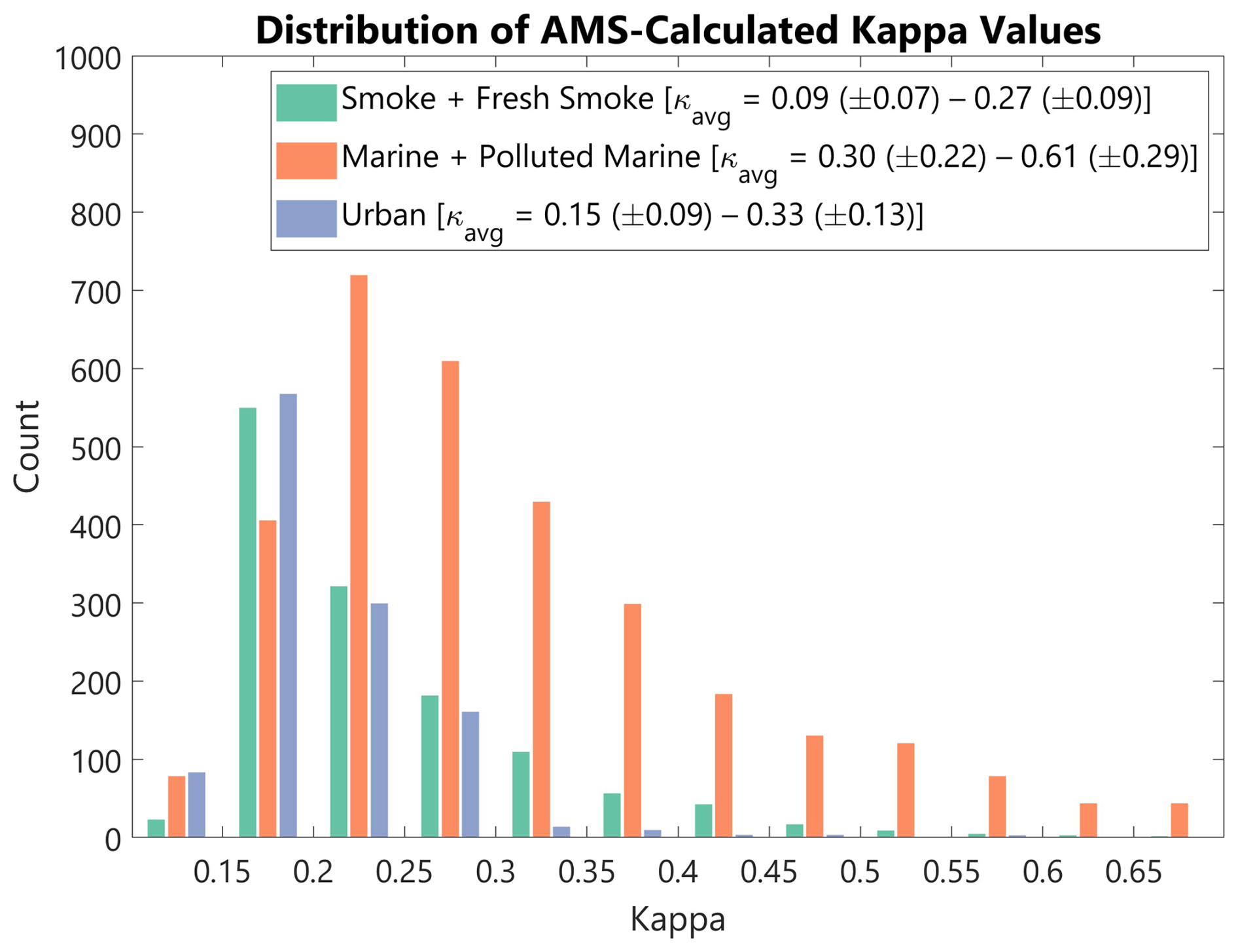
Figure 3 Distribution of kappa values calculated using the methodology in Sect. 2.3.1 for each aerosol type. Literature-averaged ranges, with the standard deviation, for each aerosol type are given in parentheses.

3.2.2 Critical diameter (D_crit) and CCN_theory calculation

After calculating kappa following the methodology in Sect. 3.2.1, we use Eq. (1) to calculate D_crit, and we calculate CCN_theory using Eq. (4):

$$\begin{array}{}\text{(4)}& {\mathrm{CCN}}_{\mathrm{theory}}\left(S\right)={\int }_{D_{\mathrm{crit}}}^{D_{max}}{\displaystyle \frac{\mathrm{d}N}{\mathrm{dlog}{D}_{\mathrm{p}}}}\mathrm{dlog}{D}_{\mathrm{p}},\end{array}$$

where D_max signifies the diameter of the largest bin from the combined SMPS and LAS number size distribution (Schmale et al., 2018; Patel et al., 2024), d$N/\mathrm{d}\log D_{\mathrm{p}}$ represents the number concentration of aerosols in each bin of the combined size distribution, and S is the CCN counter supersaturation. For direct comparisons between CCN_theory and CCN_obs, we use the exact CCN counter supersaturation value reported for each collocated data point within a small range of 0.36 %–0.38 % (Sect. 4.1). For analyses using only CCN_theory without a comparison to CCN_obs, we use a constant 0.37 % supersaturation (Sect.  4.2–4.3).

3.3 Mie calculations

The properties of light scattered by atmospheric aerosols are described by Mie theory, where aerosols are assumed to be homogeneous and spherical and to have a diameter approximately equal to the wavelength of incident radiation (Mie, 1908). For our calculations of BSC_theory, we calculate size-resolved particle backscattering efficiencies (Q_bsc) using the Mie scattering program by Bohren and Huffman (1998), implemented in the libRadtran library of radiative transfer routines and programs (Emde et al., 2016). The three inputs needed to calculate Q_bsc are particle size, complex refractive index, and wavelength. To correspond to BSC_obs, we only use a wavelength of 532 nm. We use typical refractive index values as retrieved by the Aerosol Robotic Network (AERONET) for different aerosol types to inform our refractive index selection (Dubovik et al., 2002), with exact values given in Table B1.

For particle size input, we use the SMPS and LAS size distribution bin diameters. However, here we must account for a significant difference in terms of how in situ and HSRL-2 observations are made. With these BSC_theory calculations, we want to model ambient BSC_obs from the HSRL-2 to understand the relationship with in situ CCN_obs. However, since in situ instruments dry ambient air before collecting measurements, we need to account for the change in particle diameters due to water uptake at ambient RH conditions since particle size has a significant impact on the magnitude of light scattered. Calculations made to account for changes in particle diameter and refractive index due to hygroscopic growth are outlined in Appendix B. After these adjustments, humidified bin diameters (D_wet) and refractive index components (m_wet and n_wet) are the final inputs into the Mie scattering calculations run in libRadtran. The size-resolved Q_bsc values returned from these calculations are used to calculate BSC_theory at 532 nm from the full aerosol size distribution, as shown in Eq. (5):

$$\begin{array}{}\text{(5)}& {\mathrm{BSC}}_{\mathrm{theory}}={\int }_{r_{\mathrm{1}}}^{r_n}\mathit{\pi }{r}_{\mathrm{wet}}^{\mathrm{2}}{Q}_{\mathrm{bsc}}n\left(r_{\mathrm{wet}}\right)\mathrm{d}{r}_{\mathrm{wet}},\end{array}$$

where r_wet is each humidified bin radius, n(r_wet)dr_wet represents the aerosol number concentration in each bin, and r_n represents the largest bin in the SMPS and LAS combined and humidified size distribution. This set of calculations is done using the collocation-averaged size distribution data associated with each collocated data point.

3.4 Data filtering

All input data for κ–Köhler and Mie calculations come from the collocated data set used for the observational analysis in Sect. 2. Each collocated data point contains an average value of CCN_obs and BSC_obs, as well as an average combined SMPS and LAS size distribution and set of AMS observations. Therefore, to enable a direct comparison between CCN_theory and CCN_obs, as well as between BSC_theory and BSC_obs, this collocated data set is used throughout the entirety of the study. In this section, we describe several filtering steps that are performed to minimize potential errors in the subsequent analyses. Some are motivated by the observational methodology taken in L23, and others are specific to the CCN_theory and BSC_theory calculations. All steps are summarized in Fig. 4.

We begin with the filtering criteria applied to data in the CCN_obs–BSC_obs relationships shown in Sect. 2. Since these data points are the basis for the rest of the analysis, each of these filtering steps also applies to data used for calculating CCN_theory and BSC_theory. As we are analyzing these relationships by aerosol type, we start by removing observations from the collocated data set where an HSRL-2 Aerosol ID is not determined, which typically occurs if the full set of HSRL-2 observables is not available. This step removed 51 % of the collocated data set. Additionally, we remove any points where the collocation method averages across varying Aerosol IDs to avoid introducing additional uncertainty into the aerosol type. Similarly, we remove points where the standard deviation is greater than the mean of the CCN concentration that falls within our collocation criteria to avoid potential errors due to large variability or gradients in aerosol concentration. Lastly, we remove any collocated points where fewer than two samples comprise the average. This is done to reduce potential noise in the data set, especially for the in situ size distribution data that have a critical role in both sets of theoretical calculations. In general, collocated data points represent an average of 10 observations from the 1 s merged in situ data files, some of which have a lower original resolution (Table 1). Each of these filtering steps is applied to all of the data in this study, and the impact of each step on the total number of collocated data points is shown in Fig. 4.

In L23, we found that the correlation between CCN concentration and HSRL-2 observations was strongest for supersaturations greater than 0.25 %. Additionally, since CCN depends strongly on supersaturation, we limit observations to a small range of supersaturation values to reduce additional variability. Therefore, for analyses that are strictly observational (Sect. 2) or that compare theoretical calculations with observations (Sect. 4.1), we limit our collocated data set to a supersaturation range of 0.36 %–0.38 %. This range was chosen due to the fact that a supersaturation of 0.37 % is the most frequent value used during ACTIVATE. This step is only applied to analyses that include observations because, for calculations of CCN_theory, we apply a constant supersaturation of 0.37 % to any observed size distribution. That is, we do not unnecessarily limit the data used for theoretical calculations by filtering according to CCN counter supersaturation.

The last data-filtering step serves as a check of CCN_theory calculations. In addition to using Eq. (1) to calculate D_crit, as described in Sect. 3.2, we also use an estimation method to validate κ–Köhler calculated values. This method integrates the combined SMPS and LAS number size distribution from the largest to smallest bin diameters until the difference between the summed aerosol concentration and observed CCN concentration reaches a minimum. We refer to the bin diameter where this difference reaches a minimum as the estimated D_crit (D_crit,est). We compare these values to the κ–Köhler calculated values (D_crit,calc) and require that D_crit,calc values fall within ±20 % of the D_crit,est values. This step ensures that our calculated CCN_theory values will closely match CCN_obs values and removes size distributions that may have higher noise or several bins with missing concentrations. The threshold of ±20 % is chosen to correspond to the SMPS and LAS reported uncertainty that impacts the accuracy of the D_crit,est value. This step applies to all analyses involving calculations of CCN_theory and BSC_theory (Sect. 4).

As seen in Fig. 4, some of these steps remove a significant amount of data from the analysis. While the amount of data removed was taken into consideration at each step, all steps were taken as a precaution against introducing anomalous variation and uncertainty into the analysis. The application of slightly different combinations of filtering steps to the analyses in Sect. 4 was done intentionally to allow for as much data as possible to be included in each step. Therefore, while the D_crit agreement filtering step is applied everywhere where we calculate CCN_theory and BSC_theory, the CCN counter supersaturation filter is only applied where it needs to be used to control the supersaturation dependence of CCN_obs. Since the goal of this study is to understand the relationship between CCN_obs–BSC_obs through the lens of the theoretical calculations, removal of extraneous noise and variability from the input data allows for analyses to more accurately determine the true underlying factors governing the CCN_theory–BSC_theory relationship. We discuss a comparison between observed and theoretically calculated CCN and BSC in Sect. 4.1, but a detailed discussion of closure for these variables is beyond the scope of this study.

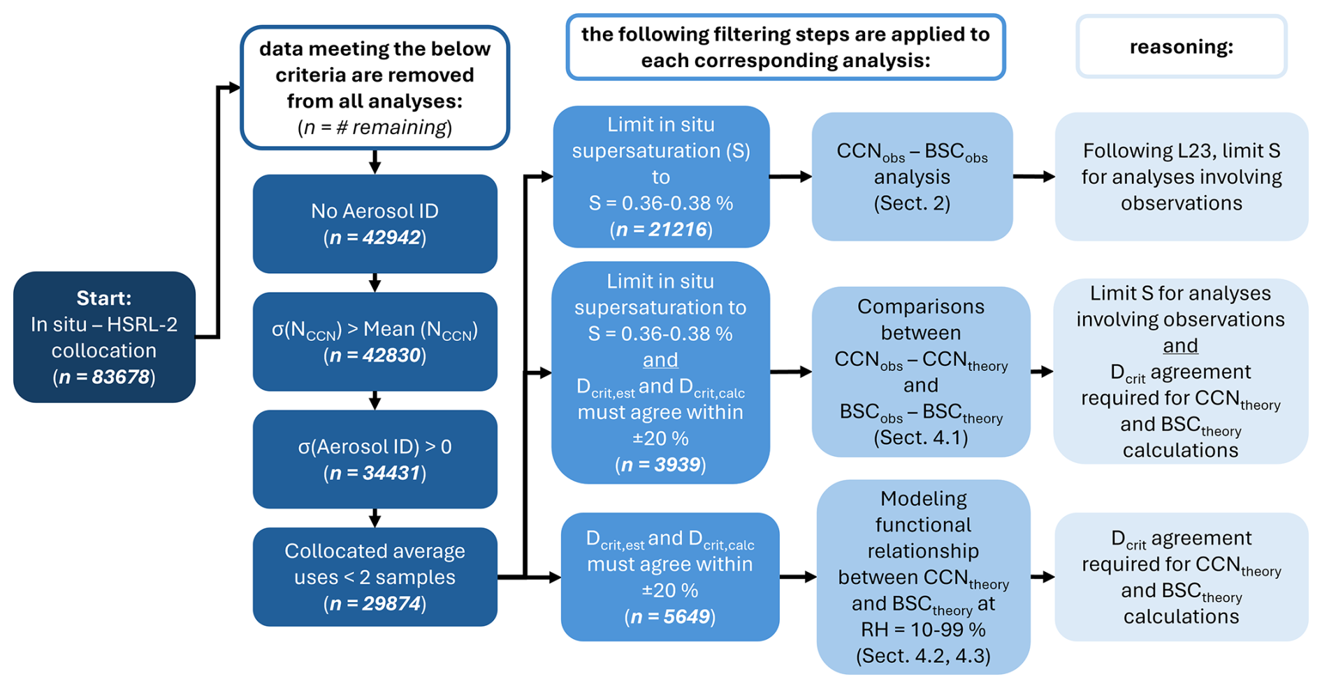
Figure 4 Flowchart describing the data-filtering steps applied to data for all analyses and filtering steps applied to data for specific analyses. The number of points remaining after each step (n) is given in parentheses. Therefore, approximately 25 % of the original number of collocated samples remain for the observational analysis in Sect. 2, 5 % remain for analyses comparing observations and theoretical values in Sect. 4.1, and 7 % remain for purely theoretical analyses in Sect. 4.2 and 4.3.

4 Results

4.1 CCN and BSC observations vs. calculations

We first calculate CCN_theory and BSC_theory under observed ambient conditions and compare calculations to observations. CCN_theory is calculated for all data using the corresponding CCN counter supersaturation, and BSC_theory is calculated from humidified aerosol size distributions using the corresponding observed RH value. Since this step involves theoretical calculations and comparison with observations, we limit the data set to observations made at CCN counter supersaturation between 0.36 %–0.38 % and apply the D_crit agreement filtering step (Fig. 4).

The comparison between CCN_obs and CCN_theory is given in Fig. 5. We show results requiring a D_crit agreement outlined in gray, while calculations without this requirement are plotted in the background. Results for calculations not requiring D_crit agreement are shown to demonstrate how this requirement impacts the data set. Results of a linear regression between CCN_obs and CCN_theory for data requiring the D_crit agreement show that, for all aerosol types, R² ranges from 0.91 to 0.94, and RMSE ranges from 87 to 133 cm⁻³. These RMSE values are very close to the approximate median value of CCN uncertainty of 150 cm⁻³. Data are generally clustered very close to the 1:1 line for all aerosol types, and the lines of best fit also fall close to the 1:1 line. Overall, this analysis gives us confidence that our methodology accurately calculates CCN_theory as a necessary precursor for the correlation analysis with BSC_theory.

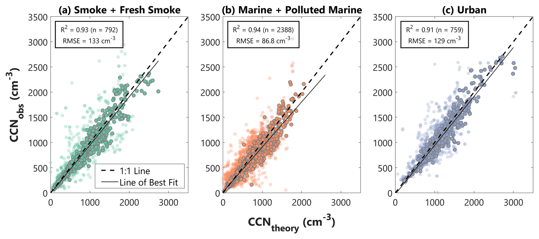
Figure 5 CCN_obs vs. CCN_theory for (a) smoke and fresh smoke, (b) marine and polluted marine, and (c) urban aerosols. The 1:1 lines are dashed, and the lines of best fit for the linear regressions between both variables are solid. Markers outlined in gray denote results for calculations requiring a certain level of D_crit agreement. Results for calculations not requiring a D_crit agreement are shown in the background with lighter transparency to demonstrate how this requirement impacts the data set.

The same statistics are shown for our comparison between BSC_obs and BSC_theory at 532 nm in Fig. 6, where marker colors correspond to RH to show the impact of hygroscopic growth on calculated BSC_theory. Here, our R² values range from 0.45 to 0.75, and RMSE ranges from $\mathrm{2.7}\times {\mathrm{10}}^{-\mathrm{4}}$ to $\mathrm{1.6}\times {\mathrm{10}}^{-\mathrm{3}}$ km⁻¹ sr⁻¹. We find that the performance of our calculations does not appear to systematically decline for observations made at high RH, providing confidence in our humidification calculation methods. The R² and RMSE values indicate a weaker correlation between observations and calculations than for CCN, but data remain primarily clustered around the 1:1 line. While the use of the D_crit filtering step for this analysis and subsequent removal of size distributions with higher noise or missing concentrations does benefit BSC_theory calculations, this does not force a degree of agreement between BSC_obs and BSC_theory in the same way as it does for agreement between CCN_obs and CCN_theory. Additionally, CCN_obs and the inputs for the CCN_theory calculation all come from in situ observations, while the BSC_theory calculation uses in situ observations as input but is compared to BSC_obs from remote sensing instrumentation on a separate platform. Varying resolutions and collocation averaging between in situ and HSRL-2 observations may cause discrepancies between BSC_obs and BSC_theory. Other discrepancies in the BSC_theory calculation may come from approximations including the Mie theory assumption of spherical particles and our use of literature-averaged refractive index values for different aerosol types. As with the CCN comparison (Fig. 5), this analysis also gives us confidence that our methodology results in BSC_theory values of a similar magnitude as BSC_obs.

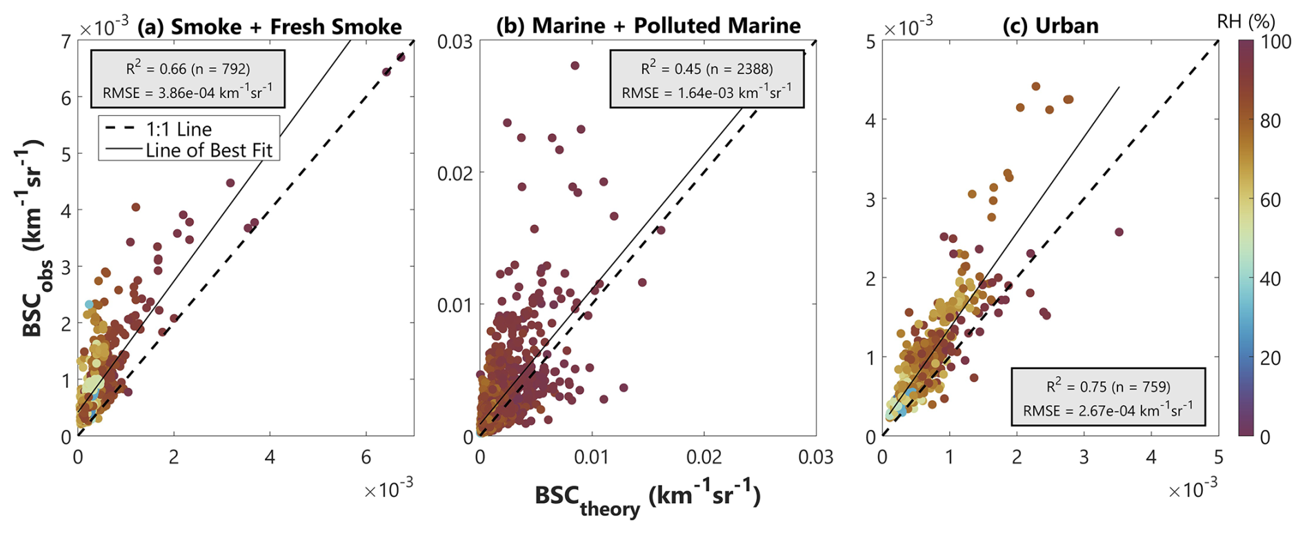
Figure 6 BSC_obs vs. BSC_theory at 532 nm for (a) smoke and fresh smoke, (b) marine and polluted marine, and (c) urban aerosols. The 1:1 lines are dashed, and the lines of best fit for the linear regressions between both variables are solid. Marker colors correspond to ambient RH that was observed by each BSC_obs and applied to calculate each corresponding BSC_theory.

4.2 Estimating predictor importance

In investigating the CCN_obs–BSC_obs relationship for different aerosol types, we determined that a linear regression is not an appropriate model for the ACTIVATE data (Fig. 2). Additionally, we have shown reasonable agreement between CCN_obs and CCN_theory and between BSC_obs and BSC_theory at ambient conditions. Next, we use the theoretical calculations to investigate and interpret the causes of scatter and non-linearity in the CCN_obs–BSC_obs relationship. Analyses in this and the next section use CCN_theory calculated at a constant supersaturation of 0.37 %.

Recall that the three main factors influencing how CCN concentration relates to AOPs are ambient RH, the shape of the aerosol size distribution, and aerosol chemical composition. Due to the highly interconnected nature of these factors and their relationships with CCN and BSC, we use random forest (RF) models to determine the relative importance of each factor in controlling the CCN_theory–BSC_theory relationship. A random forest is an ensemble of decision trees where each tree is created using the best split from a randomly selected subset of predictors. The final prediction comes from a majority vote among individual trees (Breiman, 2001; Hu et al., 2017). This method was chosen due to its high accuracy, generalization capability, ability to handle non-linear relationships between features, and ability to provide estimates of predictor importance. Another benefit of this method is the ability to consider all input variables collectively as opposed to investigating or perturbing individual input variables one at a time. For each model, we use 200 ensemble learning cycles and specify that all predictor variables are used at each node to ensure that each tree uses all predictor variables. Additionally, 10-fold cross-validation is used during training to prevent overfitting by any single model. The final predictor importance is determined by averaging the importance estimates across the 10 models, and the standard deviation is used to reflect the variations in the final calculated predictor importance estimates. Additionally, we do not separate our data into training and testing subsets because our purpose is not to train and refine a model that predicts CCN_theory or the CCN_theory–BSC_theory relationship. Redemann and Gao (2024) provide a well-tested machine learning method with which CCN concentration is predicted from several HSRL-2 and reanalysis input variables. Rather, here, we use RF predictor importance as a tool to help investigate the impact that ambient RH, aerosol size distribution, and aerosol chemical composition each have on the CCN_theory–BSC_theory relationship.

We use a combination of observed effective radius (R_eff), geometric mean radius (GMR), RH, and kappa as predictors of the CCN_theory : BSC_theory ratio in our RF models. Effective radius is the ratio of the third and second moments of the aerosol size distribution, sometimes called the area-weighted mean radius. This makes it useful for optical measurements as the energy removed from light by an aerosol is proportional to its area. Effective radius is calculated using Eq. (6):

$$\begin{array}{}\text{(6)}& R_{\mathrm{eff}}={\displaystyle \frac{{\int }_{\mathrm{0}}^{\mathrm{\infty }}\mathit{\pi }{r}_{\mathrm{wet}}^{\mathrm{3}}n\left(r_{\mathrm{wet}}\right)\mathrm{d}{r}_{\mathrm{wet}}}{{\int }_{\mathrm{0}}^{\mathrm{\infty }}\mathit{\pi }{r}_{\mathrm{wet}}^{\mathrm{2}}n\left(r_{\mathrm{wet}}\right)\mathrm{d}{r}_{\mathrm{wet}}}},\end{array}$$

where r_wet is the humidified particle radius, and n(r_wet)dr_wet is the aerosol concentration within each bin of the humidified size distribution. The geometric mean radius is the mean of the humidified aerosol size distribution in log space, as given by Eq. (7):

$$\begin{array}{}\text{(7)}& \mathrm{GMR}=\left({\displaystyle \frac{{\int }_{\mathrm{0}}^{\mathrm{\infty }}\ln r_{\mathrm{wet}}n\left(r_{\mathrm{wet}}\right)\mathrm{d}{r}_{\mathrm{wet}}}{N_{\mathrm{0}}}}\right),\end{array}$$

where N₀ is the total number of particles in the size distribution. It is important to note that the predictors used in this analysis are not fully independent. For example, RH impacts R_eff depending on the corresponding kappa value, meaning that the influence of RH on the CCN_theory–BSC_theory relationship may be captured through R_eff. However, we include both parameters separately to investigate if one of these variables is more important than the other in constraining the CCN_theory–BSC_theory relationship. Additionally, both R_eff and GMR capture the shape of the size distribution and can be related through functional relationships. We use R_eff and GMR separately because of their different information content. The weighting of R_eff toward larger particles increases its relevance for AOPs, while GMR tends to fall within the fine mode of the size distribution closer to D_crit and aerosol sizes relevant for CCN activation. Therefore, based on this combination of input variables, we train the RF models to predict the ratio of CCN_theory : BSC_theory.

First, we train a model for all aerosol types combined. Here, the Aerosol ID from our collocated in situ and remote sensing data set is added as an additional predictor to test the dependence of CCN_theory : BSC_theory on lidar-indicated aerosol type. Average relative predictor importance estimates across all 10 folds are shown in Fig. 7a, with a standard deviation designated for each average. Overall, R_eff is determined to be the most important predictor of CCN_theory : BSC_theory, followed by RH. Aerosol ID is the third most important predictor, and GMR and kappa are approximately equal as the fourth and fifth most important predictors, respectively.

Next, we train three individual models that predict CCN_theory : BSC_theory for each individual aerosol type as separated by Aerosol ID and again average the relative predictor importance estimates across all 10 folds (Fig. 7b). We find that, after separating aerosol types, R_eff remains the most important predictor of CCN_theory : BSC_theory for all aerosol types. Kappa ranking least important for each aerosol type indicates that separating aerosol types using the Aerosol ID adequately constrains the impact of aerosol chemical composition on the CCN_theory–BSC_theory relationship. These separate models also indicate that RH is the second most important predictor for all aerosol types. The relatively low importance of Aerosol ID and kappa in these models is expected considering the fact that BSC_theory is primarily determined by aerosol size and that CCN activation is also more sensitive to size than to aerosol chemical composition (Dusek et al., 2006).

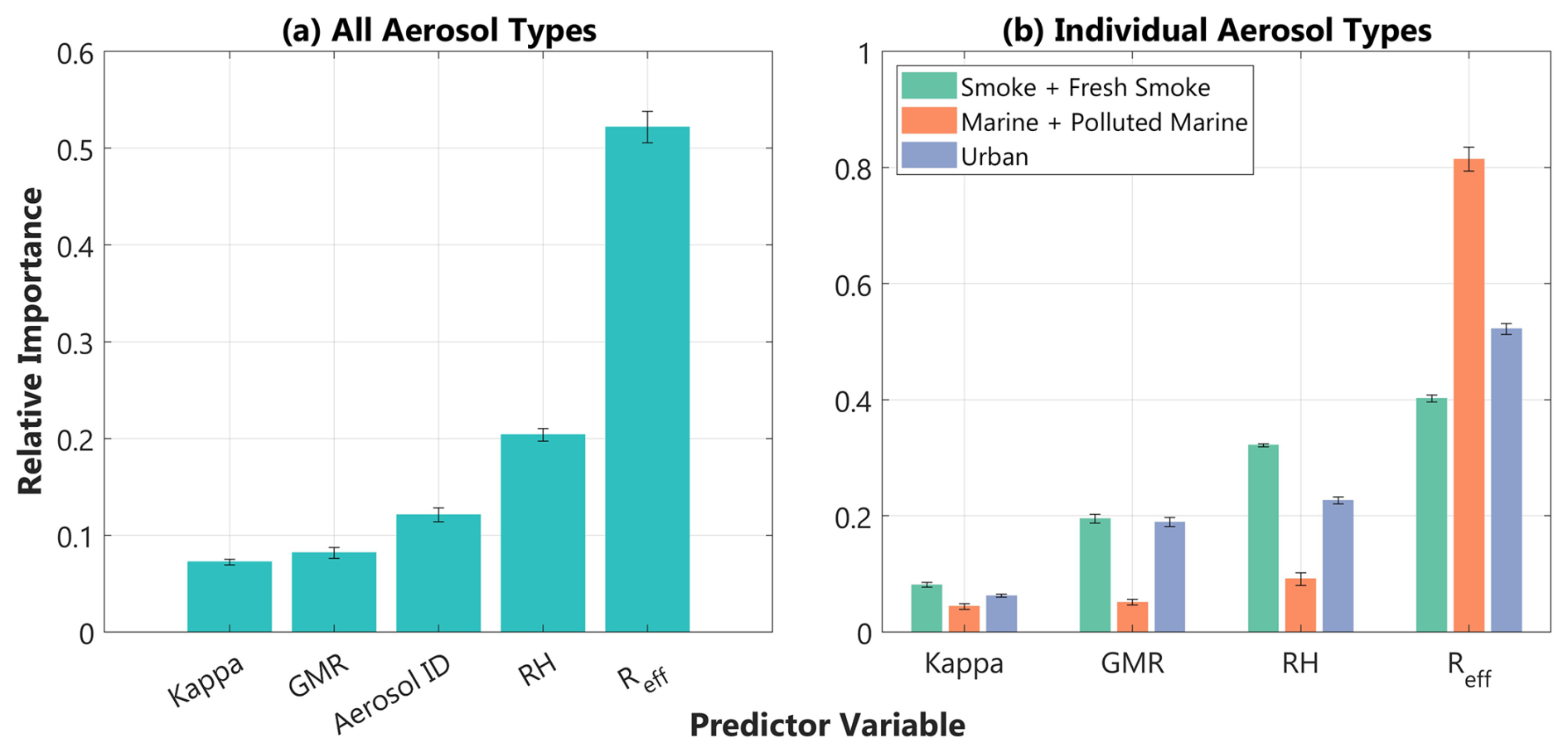
Figure 7 Average random forest predictor importance estimates across 10-fold cross-validation for (a) the model run for all three aerosol types combined and (b) individual models run for the three different aerosol types. Each model predicted the CCN_theory : BSC_theory ratio based on the observed input variables listed on each x axis. All importance estimates are relative. Error bars designate standard deviation across the 10-fold cross-validation.

4.3 Modeling CCN_theory : BSC_theory using effective radius

Based on the RF predictor importance estimate indication that R_eff is the most important predictor for the CCN_theory–BSC_theory relationship compared to RH, kappa, and GMR (Fig. 7), we now investigate the physical relationship between R_eff and the CCN_theory : BSC_theory ratio. We focus on R_eff to further explore and understand the RF indication of its high importance compared to the other predictors and to understand how much variance in CCN_theory : BSC_theory can be explained by R_eff alone.

We start by humidifying each dry aerosol size distribution at 10 % RH increments from 10 % to 99 % and calculating CCN_theory, BSC_theory, and R_eff from each humidified size distribution. This process allows us to model all variables for a wide range of plausible environmental RH values that are not constrained to observed ambient conditions and to form a more comprehensive understanding of the underlying physical relationship between R_eff and CCN_theory : BSC_theory. When comparing CCN_theory : BSC_theory and R_eff, we fit two-term exponential curves for each aerosol type to represent the relationship (Fig. 8). A two-term exponential was chosen for each aerosol type due to a slightly higher R², lower RMSE, and better visual fit to the larger R_eff values than a one-term exponential fit. For each aerosol type, we provide the R² and RMSE (Fig. 8), and fit coefficients are provided in Table 2.

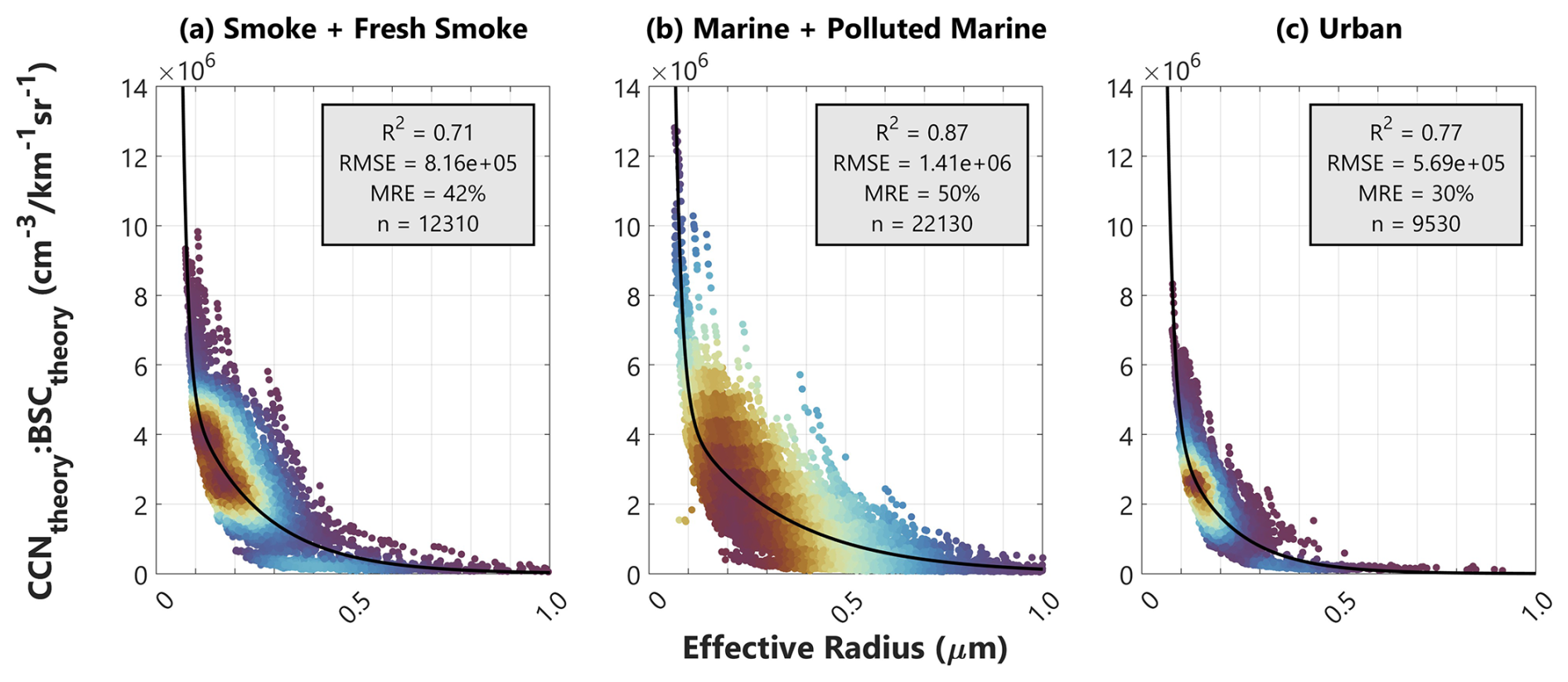
Figure 8 CCN_theory : BSC_theory vs. R_eff for (a) smoke and fresh smoke, (b) marine and polluted marine, and (c) urban aerosols. Marker colors correspond to the density of surrounding points, with red shades indicating high density and blue shades indicating lower density. The black line represents the two-term exponential curve fit for each aerosol type. The R², RMSE, mean relative error (MRE), and number of data points (n) for each exponential fit are also provided.

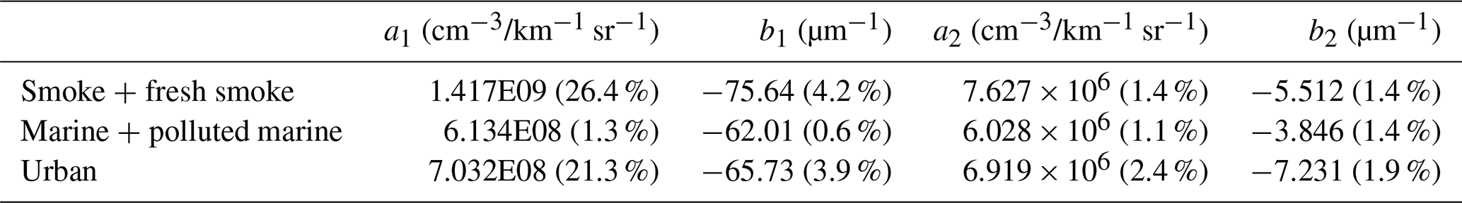
Table 2 Coefficients for the two-term exponential curves fit to each aerosol type to model the CCN_theory : BSC_theory–R_eff relationship. All fit equations take the form of $y=a_{\mathrm{1}}\exp \left(b_{\mathrm{1}}x\right)+a_{\mathrm{2}}\exp \left(b_{\mathrm{2}}x\right)$, where y corresponds to the CCN_theory : BSC_theory ratio in cm⁻³ per km⁻¹ sr⁻¹, and x corresponds to R_eff in µm. Relative uncertainties for each coefficient are given in parentheses, estimated using 95 % confidence bounds.

Next, we use each of these two-term exponential fits to calculate CCN : BSC from values of R_eff in our ambient collocated data set and compare to CCN_theory : BSC_theory. Here, we refer to CCN : BSC modeled using the two-term R_eff exponential fits as (CCN : BSC)_model to capture the fact that the ratio itself is modeled using R_eff and not each term individually and to distinguish it from CCN_theory : BSC_theory. This comparison is shown in Fig. 9, where we find that, overall, most data are clustered around the 1:1 line for each aerosol type. We see that RMSE and mean relative error (MRE) are lowest for the URB category and highest for MPM. Additionally, SFS and URB have many data points at or slightly below the 1:1 line, and a majority of (CCN : BSC)_model ratios have magnitudes of about 2 × 10⁶ to 4 × 10⁶ cm⁻³ per km⁻¹ sr⁻¹, while most values for MPM are less than 2 × 10⁶ cm⁻³ per km⁻¹ sr⁻¹. The R² values for all aerosol types range between 0.68–0.79.

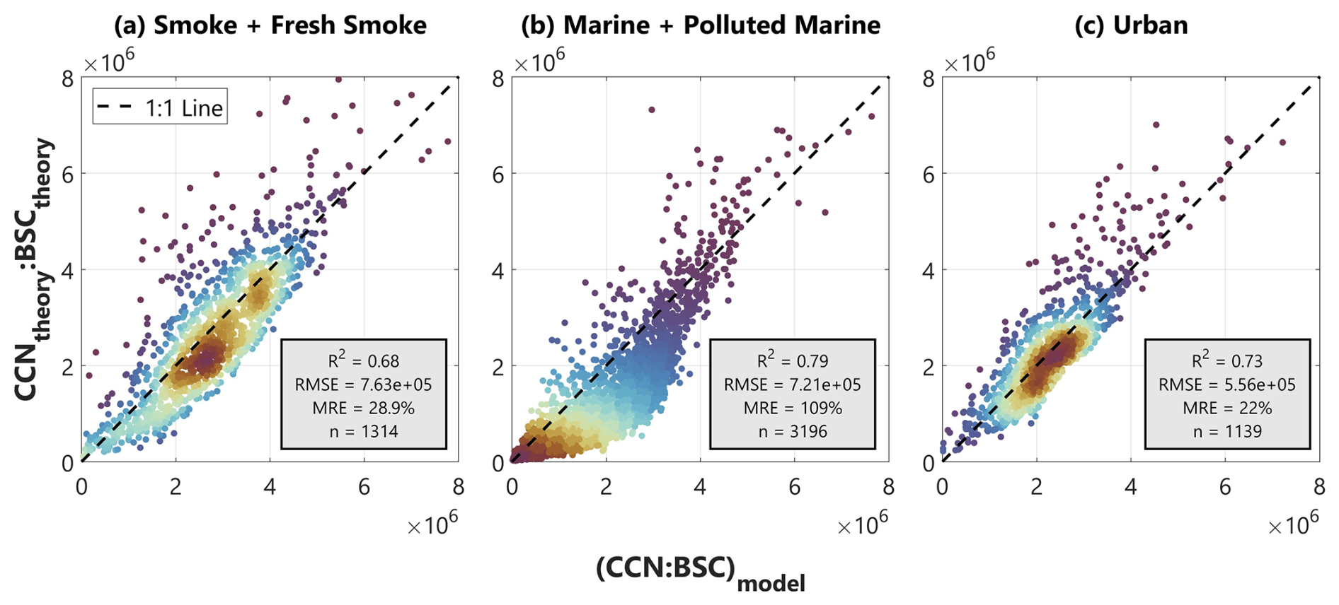
Figure 9 Comparison of CCN_theory : BSC_theory to (CCN : BSC)_model for (a) smoke and fresh smoke, (b) marine and polluted marine, and (c) urban aerosols. (CCN : BSC)_model values come from the two-term exponential fits shown in Fig. 8 and defined in Table 2. The units for both axes are cm⁻³ per km⁻¹ sr⁻¹. Marker colors correspond to the density of surrounding points, with red shades indicating high density and blue shades indicating lower density. The dashed line on each panel is the 1:1 line. The R², RMSE, MRE, and number of data points (n) for each exponential fit are also provided.

5 Discussion

Several recent studies have used lidar-observed aerosol optical properties to develop physics-based or ML (machine learning)-based parameterizations and retrieval methods for the CCN concentration of different aerosol types (Mamouri and Ansmann, 2016; Lv et al., 2018; Haarig et al., 2019; Choudhury and Tesche, 2022a; Patel et al., 2024; Redemann and Gao, 2024). In this study, we have included in situ-observed aerosol size and chemical composition information to determine which factors most strongly govern the CCN_theory–BSC_theory relationship. Therefore, this analysis provides a broad theoretical context in which relationships between observed CCN and aerosol optical properties can be interpreted. In this section, we discuss the physical interpretation of the relationships found, implications for future remote sensing techniques, and a summary of the sources of uncertainty and limitations of the study.

5.1 Physical relationships

Based on a set of predictors for the CCN_theory : BSC_theory relationship, including R_eff, GMR, kappa, and RH, RF predictor importance estimates indicated that R_eff was the most important predictor for all three aerosol types of interest in this study. Therefore, we investigated further the relationship between CCN_theory : BSC_theory and R_eff for a wide range of plausible environmental RH conditions and found a two-term exponential relationship. In further understanding this pattern, it is important to recall that R_eff is influenced more significantly by coarse-mode particles than by fine-mode particles. As the coarse-mode number concentration increases, we expect BSC_theory to increase more compared to CCN_theory, thus decreasing the CCN_theory : BSC_theory ratio. This finding is similar to that of Shen et al. (2019), where an exponential relationship was found between the CCN : AOP ratio and the geometric mean diameter of generated lognormal unimodal size distributions. Additionally, here, the exponential fits show a steeper decrease in CCN_theory : BSC_theory with R_eff for MPM aerosols compared to other aerosol types (Table 2). Since MPM aerosols are expected to have a more significant coarse-mode contribution, it appears that the effect of BSC_theory increasing more than CCN_theory with R_eff is more pronounced for this aerosol type. As previously mentioned, RH also has an impact on R_eff that depends on kappa. The indication that R_eff is the most important predictor suggests that understanding the CCN_theory : BSC_theory relationship as based on ACTIVATE observations is not as straightforward as simply constraining RH, as could be done in L23. Rather, the impact of RH on the aerosol size distribution is more important in determining how CCN_theory and BSC_theory are related.

Based on the R² values of 0.68–0.79 in our comparison of CCN_theory : BSC_theory and (CCN : BSC)_model (Fig. 9), we find that modeling CCN_theory : BSC_theory using two-term exponential R_eff relationships can explain approximately 68 %–79 % of the variance in the CCN_theory–BSC_theory relationship. While we previously hypothesized in L23 that aerosol hygroscopic growth at high ambient RH may be the leading cause of variability when relating CCN_obs and BSC_obs, here, we find that most variability is attributable to differences in R_eff. Furthermore, this analysis also speaks to inherent differences in how CCN_theory relates to BSC_theory for different aerosol types. We find that, when using a large set of actually observed aerosol size distributions as the input into theoretical calculations, there is a significant difference in the range of possible R_eff values for each aerosol type (Fig. 8). For example, many MPM observations span a wide range of R_eff between approximately 0.1–0.5 µm, while SFS and URB, even at wide range of possible ambient RH, primarily see R_eff values limited to a small range between 0.1–0.2 µm. Additionally, when we look at the magnitude of CCN_theory : BSC_theory values for each aerosol type, MPM tends to have much lower values than SFS and URB (Fig. 9). Higher R_eff values, in addition to a higher likelihood for hygroscopic growth in humid marine environments, act to increase BSC_theory more than CCN_theory, thus decreasing the CCN_theory : BSC_theory ratio more than for other aerosol types.

Here, we present three CCN_theory : BSC_theory–R_eff exponential fits as a methodology for explaining variance in the CCN_theory–BSC_theory relationship. The exact functional forms presented in Fig. 8 are most appropriate for ACTIVATE observations, and the coefficients would likely need to be adjusted before applying to other data sets. While we expect the general exponential pattern to hold for other data sets, any differences in observed aerosol size distribution or chemical composition would likely change the exact fit coefficients.

5.2 Implications for remote sensing techniques

This study indicates several important considerations for future work constraining CCN concentrations from remote sensing observations and future spaceborne lidar data sets. Most importantly, given our finding that particle size, as parameterized by R_eff, is the most important predictor in determining the CCN_theory–BSC_theory relationship, two key points are suggested. First, a simple linear approximation with BSC_obs will not constrain CCN_obs well in most cases in the ACTIVATE data set. Many previous studies have suggested that the relationship between CCN concentration and various AOPs is often non-linear, specifically for AOD. Considering this background, the results presented here suggest that variations in aerosol size distribution may be a leading cause of non-linearity when using AOD as a proxy for CCN concentration. Seemingly in contrast with the results presented here, in L23, we investigated the relationship between CCN concentration and aerosol index (AI), an indicator of particle size, and found little to no difference between CCN–AI and the CCN–EXT or CCN–BSC relationships. Therefore, for observations of smoke at low RH over the ORACLES region, we concluded that there was a very small variation in aerosol size in the observations. With minimal differences in aerosol size and with most smoke plume observations being made at low ambient RH, conditions permitted a simple linear approximation to relate CCN_obs and BSC_obs. On the contrary, the larger data set from the ACTIVATE campaign is characterized not only by a variety of aerosol types but also by a wider range of aerosol size distributions and a higher fraction of observations made at high ambient RH in the MBL, all of which contribute to increased non-linearity between CCN_obs and BSC_obs.

Related to this non-linearity, a second key point from this analysis is that, in most cases, efforts to constrain CCN concentration using AOPs need to include a measure of the aerosol size distribution to accurately represent variability in the relationship. Here, we have taken advantage of the availability of in situ aerosol size distributions and represented them using R_eff. However, to constrain CCN concentration solely from spaceborne lidar observations, our findings suggest that either satellite retrievals of R_eff would need to be collocated with lidar observations or a different lidar-derived indicator of aerosol size would need to be used. For example, AI can be calculated using two wavelengths of aerosol extinction from lidar, and other multi-wavelength parameters such as the lidar ratio or backscatter color ratio contain information about aerosol size that could be tested in place of R_eff for future methods based solely on a spaceborne lidar system. Additionally, R_eff retrievals from the recently launched SPEXone multi-angle polarimeter on board the NASA Plankton, Aerosol, Cloud, and ocean Ecosystem (PACE) mission (Hasekamp et al., 2019) are another option for quantifying aerosol size in CCN concentration estimates.

Lastly, when predicting CCN_theory : BSC_theory for all aerosol types combined, the RF predictor importance estimates indicated that aerosol type, as represented by the HSRL-2 Aerosol ID, is the third most important predictor (Fig. 7a). Since the Aerosol ID product categorizes aerosol types based on HSRL-2 optical properties, such as BSC, this may explain why Aerosol ID is estimated to be a more important predictor of CCN_theory : BSC_theory than kappa in terms of aerosol type and chemical composition. This finding, in addition to the qualitative differences seen in the impact of high RH between aerosol types (Fig. 4), suggests that, while Aerosol ID is not the most important predictor, separately analyzing the CCN–BSC relationship for different aerosol types provides insight into physical differences in CCN–AOP relationships between aerosol types.

5.3 Sources of uncertainty and limitations

There are several assumptions underlying both κ–Köhler and Mie theories in addition to uncertainties associated with the observations used as input. Individual instrument uncertainties are discussed in Sect. 2.1, and calculation assumptions are discussed in Sect. 2.3 and 2.4. Here, we acknowledge the primary sources of uncertainty underlying this analysis and the limitations in its applicability.

First, the most significant sources of uncertainty come from uncertainty associated with in situ observations. For example, we use AMS observations to calculate a bulk kappa value needed for κ–Köhler calculations. While we find that our calculated values are generally close to those found in the literature for all three aerosol types (Fig. 2), there are a variety of factors that may cause discrepancies. For example, the fraction of mass observed at sizes close to D_crit is generally small, meaning that AMS sensitivity to chemical composition at relevant CCN sizes can be limited. Additionally, κ–Köhler theory assumes that chemical composition is fixed across all aerosol sizes (Petters and Kreidenweis, 2007), which may cause discrepancies between CCN_obs and CCN_theory. Additionally, Kim et al. (2017) found that CCN closure using AMS-calculated kappa values was less accurate than when using kappa calculated from humidified tandem differential mobility analyzer (HTDMA) observations.

We also consider observational uncertainty associated with in situ size distributions that impact both CCN_theory and BSC_theory calculations. For example, when considering the comparison between BSC_obs and BSC_theory, we see the lowest R² for the MPM comparison (Fig. 6b), for which we present two possible causes. First, marine aerosols have a greater tendency compared to smoke and urban aerosols to be non-spherical in shape, as was observed over Barbados by Haarig et al. (2017) and as has been discussed for the ACTIVATE data set by Ferrare et al. (2023), while Mie theory assumes that particles are spherical (von Hoyningen-Huene and Posse, 1997; Bi et al., 2018). Second, in situ aerosol size distributions tend to underrepresent coarse-mode aerosols due to inefficient sampling at large sizes (McMurry, 2000; Ryder et al., 2018; Kangasluoma et al., 2020). Since marine aerosols tend to have a dominant coarse mode that contributes significantly to light scattering and since this coarse mode is likely to be underrepresented by the in situ size distributions used as input into Mie calculations, this may be another cause of the discrepancy between BSC_obs and BSC_theory. Lastly, aerosols may be undersized due to the loss of volatile aerosol components that occurs during the heating and drying of in situ observations during inlet transmission (Shrestha et al., 2018; Sandvik et al., 2019), and this may be another source of uncertainty in BSC_theory and CCN_theory calculations. However, overall, Figs. 5 and 6 provide confidence that the combination of uncertainties in the size distributions and other input variables does not prohibit reasonable agreement between CCN_obs and CCN_theory or between BSC_obs and BSC_theory. Therefore, while uncertainties in the in situ data are likely to cause errors in our theoretical calculations, the intermediate comparison between observations and calculations provides confidence that these uncertainties do not undermine the validity of this study.

Lastly, there are a few important considerations for the applicability and limitations of this study. While the ACTIVATE campaign collected one of the most complete airborne data sets in terms of the range of aerosol types and meteorological conditions, our findings are limited to the campaign study area and the encountered aerosol mixtures; they have not been tested on other data sets. For example, since we are unable to include dust in the analysis due to observational constraints, our results cannot speak to differences in the CCN_theory–BSC_theory relationship for aerosol mixtures with large proportions of dust. We would expect the results shown here to differ for observations of dust due, in part, to its hydrophobic nature and large, generally non-spherical sizes and shapes that are not easily represented using Mie theory. Recent studies have started using lidar products to better model and understand dust aerosol optical properties (Saito and Yang, 2021; Haarig et al., 2022), but more work is needed to understand the relationship between dust optical properties and its ability to activate as CCN. Additionally, as previously mentioned, we would also expect the general exponential relationship between CCN_theory : BSC_theory–R_eff to hold for other non-dust data sets, but the exact fit coefficients would likely need to be adjusted.

6 Conclusions

To improve our understanding of CCN distributions, many techniques have developed proxies and parameterizations using remotely sensed AOPs. Such strategies often provide a good constraint for CCN, but challenges remain due to factors such as aerosol hygroscopic growth and variations in the aerosol size distribution. In this study, we investigate the dominant governing factors of the CCN_theory–BSC_theory relationship at 532 nm for different aerosol types using observation-informed theoretical calculations and find that R_eff is the most important predictor for smoke, marine, and urban aerosols.

This dependence of CCN_theory–BSC_theory on the aerosol size distribution explains why, as expected, a linear approximation is generally not an appropriate method for representing the relationship well. Rather, this approach only works in limited, specific cases. For example, when analyzing the CCN_obs–BSC_obs relationship for observations of smoke at low ambient RH with a narrow range of aerosol sizes in ORACLES, a linear regression performed well. However, in cases such as ACTIVATE, where (i) most observations are made at high ambient RH, (ii) there is a variety of aerosol types present, and (iii) there exists a wider range of observed aerosol size distributions, this approach is not possible. Through these observation-informed analyses, we have provided a theoretical framework for understanding the impact of different governing factors on the CCN_obs–BSC_obs relationship and the relative importance of the size distribution compared to chemical composition and hygroscopic growth at high ambient RH.

Our findings suggest a few key takeaways for future studies using spaceborne remote sensing instrumentation, such as CALIPSO (Cloud-Aerosol Lidar and Infrared Pathfinder Satellite Observation) or other future spaceborne lidar observations, to retrieve CCN concentrations at cloud-relevant altitudes. Most importantly, we found through using a wide range of in situ-observed size distributions that R_eff captures well the strong dependence of the CCN_theory–BSC_theory relationship on the aerosol size distribution for non-dust aerosol mixtures. That is, for areas with a wide variety of observed size distributions, CCN cannot be estimated well from BSC without including aerosol size. Therefore, future remote sensing methods based on estimating N_CCN from particulate backscatter would require a lidar capable of providing R_eff, a backscatter lidar in combination with a polarimeter, or collocated satellite retrievals of R_eff. Overall, we found that there is great benefit in using a wide variety of in situ-observed aerosol size distributions as input for CCN_theory and BSC_theory calculations to understand, in detail, how the size distribution impacts the relationship between CCN and AOPs.

Appendix A

The AMS-measured ion concentrations of NH${}_{\mathrm{4}}^{+}$, SO${}_{\mathrm{4}}^{\mathrm{2}-}$, and NO${}_{\mathrm{3}}^{-}$ must first be converted into volume fractions as required by Eq. (3). For this conversion, we first use the simplified ion pairing scheme developed by Gysel et al. (2007) to calculate the number of moles (n) of ammonium nitrate (NH₄NO₃), sulfuric acid (H₂SO₄), ammonium bisulfate (NH₄HSO₄), and ammonium sulfate ((NH₄)₂SO₄), as outlined in Eqs. (A1)–(A5):

$$\begin{array}{}\text{(A1)}& {\displaystyle }{n}_{{\mathrm{NH}}_{\mathrm{4}}{\mathrm{NO}}_{\mathrm{3}}}=n_{{\mathrm{NO}}_{\mathrm{3}}^{-}},\text{(A2)}& {\displaystyle }{n}_{{\mathrm{H}}_{\mathrm{2}}{\mathrm{SO}}_{\mathrm{4}}}=\max (\mathrm{0},n_{{\mathrm{SO}}_{\mathrm{4}}^{\mathrm{2}-}}-n_{{\mathrm{NH}}_{\mathrm{4}}^{+}}+n_{{\mathrm{NO}}_{\mathrm{3}}^{-}}),\text{(A3)}& {\displaystyle }{n}_{{\mathrm{NH}}_{\mathrm{4}}{\mathrm{HSO}}_{\mathrm{4}}}=\min (\mathrm{2}{n}_{{\mathrm{SO}}_{\mathrm{4}}^{\mathrm{2}-}}-n_{{\mathrm{NH}}_{\mathrm{4}}^{+}}+n_{{\mathrm{NO}}_{\mathrm{3}}^{-}},n_{{\mathrm{NH}}_{\mathrm{4}}^{+}}-n_{{\mathrm{NO}}_{\mathrm{3}}^{-}}),\text{(A4)}& {\displaystyle }{n}_{({\mathrm{NH}}_{\mathrm{4}}{)}_{\mathrm{2}}{\mathrm{SO}}_{\mathrm{4}}}=\max (n_{{\mathrm{NH}}_{\mathrm{4}}^{+}}-n_{{\mathrm{NO}}_{\mathrm{3}}^{-}}-n_{{\mathrm{SO}}_{\mathrm{4}}^{\mathrm{2}-}},\mathrm{0}),\text{(A5)}& {\displaystyle }{n}_{{\mathrm{HNO}}_{\mathrm{3}}}=\mathrm{0},\end{array}$$

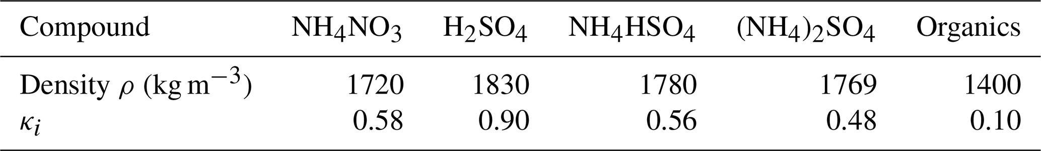
where the number of moles of NH${}_{\mathrm{4}}^{+}$, SO${}_{\mathrm{4}}^{\mathrm{2}-}$, and NO${}_{\mathrm{3}}^{-}$ is calculated using their AMS-observed ion concentrations and molar mass values. Next, the number of moles of ammonium nitrate, sulfuric acid, ammonium bisulfate, and ammonium sulfate is converted into units of mass. After this step, their dry densities, as given in Table A1 (Gysel et al., 2007; Kuang et al., 2020), are used to convert each mass into a volume. During this step, the AMS-measured concentration of organics is also converted into a volume. The five resultant volumes are summed, and the total volume is used to calculate the volume fraction (ε_i) of each component. Following this step, the individual volume fractions and κ_i values given in Table A1 (Cai et al., 2018; Kuang et al., 2020) are used in Eq. (3) to calculate a bulk kappa.

Table A1 Density and hygroscopicity constants of individual chemical components used to calculate bulk hygroscopicity value.

Appendix B

The change in particle diameter is described using a hygroscopic growth factor g(RH), as defined in Eq. (B1):

$$\begin{array}{}\text{(B1)}& g\left(\mathrm{RH}\right)={\displaystyle \frac{D_{\mathrm{wet}}\left(\mathrm{RH}\right)}{D_{\mathrm{dry}}}}.\end{array}$$

Here, D_dry is the dry particle diameter from the SMPS- and LAS-observed size distribution, and D_wet is the adjusted particle diameter at a given RH. To calculate D_wet, we follow the methodology of Zieger et al. (2013), who note that the RH dependence of Eq. (9) can be parameterized using a relationship introduced by Petters and Kreidenweis (2007), as given in Eq. (B2):

$$\begin{array}{}\text{(B2)}& g\left(a_{\mathrm{w}}\right)={\left(\mathrm{1}+\mathit{\kappa }{\displaystyle \frac{a_{\mathrm{w}}}{\mathrm{1}-a_{\mathrm{w}}}}\right)}^{\mathrm{1}/\mathrm{3}},\end{array}$$

where a_w is water activity, and κ is the bulk hygroscopicity parameter as calculated in Sect. 2.3.1. If the Kelvin effect can be neglected, a_w can be replaced with RH. Since the Kelvin term of the Köhler equation is small for large particles (D > 80 nm), we make this replacement moving forward since particles larger than 80 nm contribute most to BSC compared to smaller particles. Therefore, we calculate humidified aerosol sizes using Eq. (B3):

Table B1 Dry refractive indices for each aerosol type. The two bottom rows represent the two combined aerosol types used in this study. Their refractive indices are calculated using an average of both components from both aerosol types (i.e., the real and imaginary components for SFS are an average of the real and imaginary components for smoke and fresh smoke).

$$\begin{array}{}\text{(B3)}& D_{\mathrm{wet}}\left(\mathrm{RH}\right)=D_{\mathrm{dry}}{\left(\mathrm{1}+\mathit{\kappa }{\displaystyle \frac{\mathrm{RH}}{\mathrm{1}-\mathrm{RH}}}\right)}^{\mathrm{1}/\mathrm{3}}.\end{array}$$

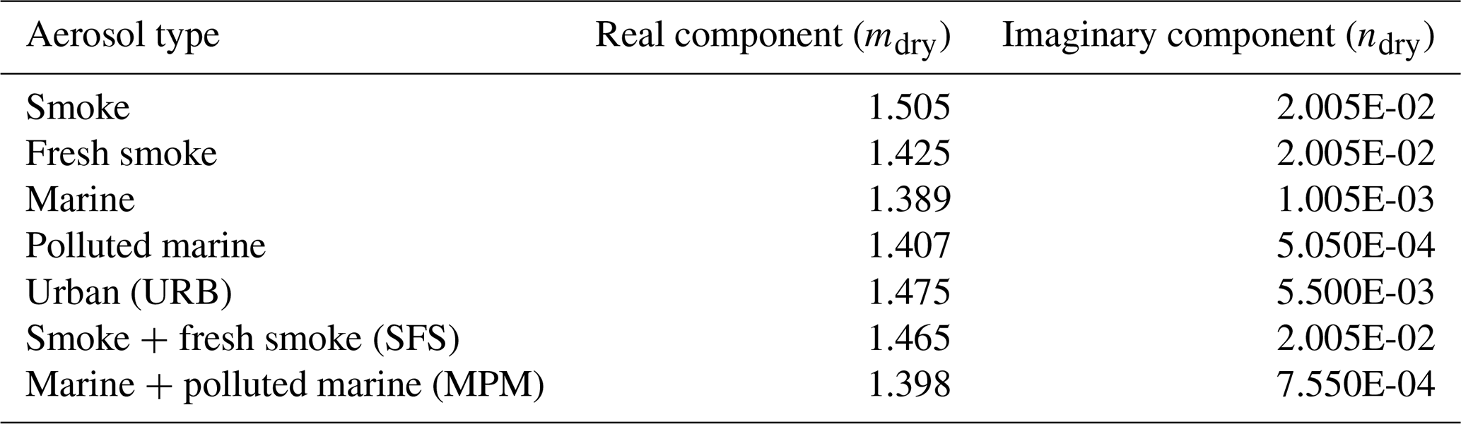
Additionally, the change in the refractive index due to hygroscopic growth is calculated using Eqs. (B4) and (B5) for the real (m_wet) and imaginary (n_wet) components, respectively:

$$\begin{array}{}\text{(B4)}& {\displaystyle }{m}_{\mathrm{wet}}\left(\mathrm{RH}\right)={\displaystyle \frac{m_{\mathrm{dry}}+m_{{\mathrm{H}}_{\mathrm{2}}\mathrm{O}}\left(g\right(\mathrm{RH}{)}^{\mathrm{3}}-\mathrm{1})}{g(\mathrm{RH}{)}^{\mathrm{3}}}},\text{(B5)}& {\displaystyle }{n}_{\mathrm{wet}}\left(\mathrm{RH}\right)={\displaystyle \frac{n_{\mathrm{dry}}+n_{{\mathrm{H}}_{\mathrm{2}}\mathrm{O}}\left(g\right(\mathrm{RH}{)}^{\mathrm{3}}-\mathrm{1})}{g(\mathrm{RH}{)}^{\mathrm{3}}}}.\end{array}$$

Here, m_dry and n_dry are the dry real and imaginary refractive indices for each aerosol type, as given in Table B1 and informed by Dubovik et al. (2002). Additionally, $m_{{\mathrm{H}}_{\mathrm{2}}\mathrm{O}}$ and $n_{{\mathrm{H}}_{\mathrm{2}}\mathrm{O}}$ are the real (1.33) and imaginary (0) refractive indices for water.