Measurement report: Microphysical and optical characteristics of radiation fog – a study using in situ, remote sensing, and balloon techniques

Based on in situ observations, remote sensing, and tethered balloon soundings, this study examines vertical profiles of microphysical and thermodynamic properties in radiative fog layers in the Strzyżów valley (Southeastern Poland). During three radiation fog events in September 2023, 74 soundings were performed, with 41 employing the OPC-N3 instrument to capture droplet spectra. All cases showed similar conditions, with liquid water path consistently above 15 g m⁻², placing most observations within the thin fog regime. Effective droplet radius decreased with height (3–4.6 µm over 100 m), while larger droplets (18.5 µm) were near the ground.

Fog dissipation occurred from both top and bottom. The mature stage showed peaks in liquid water content (LWC) and droplet number concentration (N_c) at about 80% of fog depth. Larger droplets (≥ 18.5 µm) were removed within minutes, affecting fog longevity. Equivalent adiabaticity (α_eq) – the scaling of adiabatic lapse rate to match observed liquid water path (LWP) – ranged from 0 to 0.6, with one rare case of negative near-ground α_eq. Instruments above and below the fog allowed estimation of effect of the fog's impact on radiation flux. The difference of total shortwave and longwave NET (downward − upward) radiation at ground level before and after dissipation reached 150 W m⁻². A linear relationship was found between reduction in longwave radiation and LWP under optically thin conditions. Mean LWC in the fog core ranged from 0.2–0.4 g m⁻³, and N_c reached 300 cm⁻³. Near-surface effective radius was 8–10 µm, decreasing with height. Agreement between model outputs and observed fluxes supports the retrieved microphysical parameters.

1 Introduction

A characteristic feature of radiation fogs is their localized nature, as they do not cover large areas, making their forecasting challenging. Weather conditions contribute to approximately 30 % of aviation accidents in the USA (Gultepe, 2023). Radiation fog significantly reduces visibility and complicates navigation, posing a threat to transportation. According to the American National Transportation Safety Board (NTSB), fog is the second-most-critical weather-related factor leading to fatal aviation accidents, accounting for an estimated 14 % of such incidents (Capobianco and Lee, 2001). Fog not only affects safety but also imposes significant economic costs. It can disrupt road traffic, force ships to alter their routes, and result in airport closures. In the USA, weather is the leading cause of aircraft delays, accounting for over 70 % of all cases (Kasper, 2016). Among weather-related factors, low visibility and low cloud ceilings are major contributors, as they require increased spacing between landing aircraft to maintain safety, thereby reducing airport throughput. According to NTSB data, visibility-related conditions contribute to approximately 30 %–35 % of all flight cancelations (Stevens, 2019; Gultepe, 2023).

Fog is a meteorological phenomenon occurring near the Earth's surface, characterized by the suspension of water droplets in the air, significantly reducing visibility to below 1 km (George, 1951). Several types of fog exist, depending on their formation mechanisms. This article focuses on radiation fog, which primarily forms at night under clear-sky and minimal wind conditions, within a stable boundary layer (SBL). Under such conditions, the ground surface cools significantly, leading to the cooling of the air immediately above it (Lakra and Avishek, 2022). Once the dew point temperature is reached, water vapor condenses on suspended particles (condensation nuclei), forming fog. This type of fog develops from the ground upwards, usually not exceeding 200 m in height. The cooling of successive air layers occurs from the lower layer upward, which is why radiation fogs are associated with the formation of temperature inversions. After sunrise, and with the onset of stronger winds, the fog and the inversion dissipate. When radiation fog forms, it initially remains optically thin to longwave (LW) radiation and develops within a stable lapse rate. When fog becomes optically thick, cooling occurs predominantly at the top of the fog layer, while the portion near the ground radiates in the LW range that is able to warm the surface (Mason, 1982; Price, 2011). The potential equivalent temperature becomes uniform throughout the fog layer, inducing slight instability, which in turn increases turbulence within the fog. As demonstrated by Price (2011), approximately 50 % of the fog cases he analyzed transitioned into optically thick, well-mixed fogs characterized by a saturated adiabatic stability profile. His research suggests that this conversion typically occurs when the fog layer exceeds 100 m in thickness. Numerical weather models have difficulty catching the shift from optically thin to optically thick fog (Poku et al., 2021; Boutle et al., 2022; Antoine et al., 2023).

Costabloz et al. (2025) studied fog development during the SOFOG3D experiment. They proposed several methods to identify the point at which the transition from thin to optically thick fog occurs:

• Surface LW net radiation should approach 0. In their research they assumed that this condition occurs when $\left|{\mathrm{LW}}_N\right|<\mathrm{5}$ W m⁻².

• The air temperature profile within the fog layer should decrease with height, as the air near the surface is warmed by the ground while the fog top cools radiatively. They checked whether the temperature gradient was negative by comparing temperatures at 25 and 50 m.

• Turbulent kinetic energy exceeds 0.10 m² s⁻².

• Fog top height exceeds 110 m.

• Wærsted et al. (2017) proposed that a transition to optically thick fog occurs when LWP > 30 g m⁻², but Costabloz et al. (2025) suggested a value of 15 g m⁻² to match the time when the other criteria are met more closely.

These conditions were met in the SOFOG3D experiment within about 1 h.

Key factors influencing the likelihood of fog transitioning into an optically thick state include the time of its formation (the earlier before sunrise, the more likely) and the humidity profile of the air (Boutle et al., 2018). For droplets to begin forming, aerosols acting as cloud condensation nuclei (CCN), such as ammonium nitrate aerosols, are required. In clouds, turbulence can uplift air masses, activating CCN more rapidly and extensively. In fog, droplet growth is primarily governed by radiative cooling. As demonstrated by Boutle et al. (2018), a higher concentration of large aerosol particles accelerates the transition to a well-mixed fog state. Additionally, the type of aerosol present in the air is important; compounds with high hygroscopicity that can activate at low supersaturation levels are most effective as CCN (Gilardoni et al., 2014).

According to Costabloz et al. (2025), during the SOFOG3D, inverted LWC profiles – maximum LWC found at the ground and decreasing with altitude – were commonplace in optically thin fogs. Mostly in well-mixed optically thick fogs, quasi-adiabatic profiles with LWC increasing with height were found. However, in one case, they measured LWC profiles decreasing with height 1 h after the transition occurred and LWC values at the ground reached 0.25 g m⁻³, the highest values recorded during the whole campaign.

Research utilizing cloud radars, ceilometers, and microwave radiometers has made it possible to establish the rate at which LW radiative cooling at the top of the fog layer can lead to condensation within the fog. Under clear-sky conditions, when the liquid water path (LWP) exceeds 30 g m⁻², this cooling (above the fog) can result in the formation of liquid water at a rate of up to 70 g m⁻² h⁻¹ (Wærsted et al., 2017).

The presence of clouds above the fog can also influence water condensation, with low clouds potentially blocking cooling entirely, leading to fog dissipation.

After sunrise, shortwave (SW) radiation begins to heat the fog, causing droplet evaporation. Wærsted et al. (2017) estimated that the strength of this process is about 10–15 g m⁻² h⁻¹. The rate of evaporation increases with the effective radius of droplets (r_eff) and LWP and decreases with larger solar zenith angles. Additionally, the warming of the ground surface transfers approximately 30 g m⁻² h⁻¹ of sensible heat to the fog.

To accurately predict the formation and evolution of fog, a weather forecasting model must effectively represent the interactions between the atmosphere and the Earth's surface, including various processes (such as microphysics, radiation, and turbulence), and it must do so on a local scale while accounting for terrain features.

One approach to studying fog is through large eddy simulation (LES) modeling. This approach enables the examination of turbulence effects and interactions between the atmosphere and the surface (Maronga and Bosveld, 2017), the deposition of droplets on vegetation (Mazoyer et al., 2017), or the influence of the urban canopy (Bergot et al., 2015) on fog formation and evolution. Numerical models often struggle to accurately forecast fog formation, dissipation, depth, or water content (Román-Cascón et al., 2012; Zhou et al., 2012; Bari et al., 2023). This difficulty arises from the fog's localized nature and the delicate balance between processes such as radiation balance, droplet deposition on the surface, turbulent mixing, microphysical properties, and moisture availability. Recently, AI-based tools, including machine learning and deep learning, have been employed to enhance numerical weather prediction (NWP). While these methods have shown promising results, they also introduce new challenges. Machine learning requires high-quality datasets specific to each forecast location, as well as substantial computational resources to produce timely results (Bari et al., 2023).

For the initialization of numerical models or the development of methods to retrieve LWP from satellites, it is essential to understand the microphysical properties of fog as a function of height. Unfortunately, there is a scarcity of data on the vertical distribution of fog's microphysical characteristics. Measurements using aircraft are impractical because fog typically forms close to the Earth's surface and inherently reduces visibility. However, measurements can be conducted using aerological balloons (Egli et al., 2015) and instrumentation placed on tall towers (Ye et al., 2015; Han et al., 2018), and more recently, drones and microwave radiometers (MWRs) have become viable options for such observations.

Using a tethered balloon, Pinnick et al. (1978) made the first measurements of the vertical profiles of microphysical characteristics in fog. They showed that in the studied cases, fog had a bimodal distribution of droplets (r=5 and r=0.6 µm) with a LWC range from 10⁻⁴ to 0.45 g m⁻³.

Egli et al. (2015) performed soundings with a tethered balloon and measured LWC, N_c, and r_eff every 10 m. His results from two fog cases show that the changes in LWC are related to the change in N_c and not to the change in droplet size. In most cases, r_eff was constant with height. One fog case was characterized by low LWC (maximum of 0.14 g m⁻³) but high N_c above 2000 cm⁻³. In this case of fog, three measurements were taken. Omitting the values of r_eff at the very bottom of the profiles (where the values dropped significantly), the value of r_eff decreased with height. In the case of one profile, the value of _eff at a 25 m reached a maximum of 9.4 µm. The second fog case, with six soundings, consisted of considerably thicker fog with higher LWC and r_eff values, although it was accompanied by lower total drop counts. The LWC had a constant pattern in the first third of the height, then it increased with height, and then it decreased with height to the cloud top. The highest LWC value was 0.54 g m⁻³. N_c had a similar pattern with height to LWC. The highest N_c value recorded was 500 cm⁻³. The r_eff values differ from sounding to sounding; however they were constant with height, in the range between 4 and 8 µm.

The motivation for this study is the miniaturization of equipment for particle detection. For example, the Alphasense OPC-N3, an optical particle matter (PM) sensor commonly used for aerosol monitoring, can also be used to measure the microphysical properties of fog when mounted on a tethered balloon or drone (Nurowska et al., 2023). Such a system was employed to capture vertical profiles of radiative fog in a mountain valley, a region where air pollution can be elevated during inversion conditions. This type of terrain enables fog monitoring at different altitudes. In this setup, SW and LW radiometers positioned near the valley bottom and mountain top allow determination of the optical, microphysical, and radiation closure of the fog. Section 2 outlines the instruments utilized for conducting the measurements, while Sect. 3 details the methodology of the in situ measurements and the model setup. The core of the article is presented in Sect. 4, which features a case study of radiative fog occurrence, including optical, microphysical, and radiation closure analyses performed for this case. Section 4 focuses on an event in the Strzyżów valley, where data were gathered using a balloon. The 1D Fu–Liou radiative transfer model (Fu and Liou, 1992, 1993) was applied to simulate the conditions in the Strzyżów valley, incorporating additional data from the SolarAOT station (which consists of an upper and lower station).

2 Experiment setup

This study is based on measurements taken at two sites in Strzyżów. This small town is located in southern Poland, in the region of the Strzyżowskie foothills. The city is located next to the Wisłok River. The research was conducted using remote sensing and in situ techniques as well as an apparatus connected to a tethered balloon. In addition, numerical simulations were used for the radiation closure study.

2.1 SolarAOT_lower launching site

The lower station is located in the valley of the city of Strzyżów at 260 m a.s.l. (49°52^′18.0^′′ N, 21°48^′26.0^′′ E). A CNR4 net radiometer was mounted on the site of balloon launching, for upward and downward SW and LW flux, as well as a meteo station including MetPak and sensors A100LK, W200P, HYT936, and OPC-N3. In addition, the mobile laboratory equipped with Aurora 4000 nephelometer, Laser Aerosol Spectrometer LAS 3340A, and Oxford Lasers VisiSize D30 (ShadowGraph) was used at this site. Raymetrics single-wavelength (532 nm) lidar 510M for aerosol and cloud detection was used.

The VisiSize D30 system, developed by Oxford Lasers Ltd., operates using the shadowgraph technique. The VisiSize D30, hereafter referred to as ShadowGraph, captures shadow images of particles as they pass through the measurement volume between a laser head and a high-resolution camera. This system enables the determination of microphysical properties, including particle shape, size, droplet size distribution (DSD(r)), total droplet number concentration, and liquid water content (LWC).

The ShadowGraph system has been effectively utilized in the study of cloud microphysics, both in laboratory settings and during in situ measurements. The droplet detection and sizing mechanisms of the ShadowGraph were comprehensively detailed by Nowak et al. (2021). Data collected using the ShadowGraph in studies of orographic clouds, specifically under foggy conditions in mountainous regions, were analyzed by Mohammadi et al. (2022).

During this campaign, the ShadowGraph was used for two purposes: first, as the reference instrument to which the OPC-N3 was calibrated, as demonstrated in Nurowska et al. (2023), and second, to monitor conditions near the surface. The ShadowGraph operates using a high-power laser with a wavelength invisible to the human eye. For safety reasons, it was installed on the roof of the mobile laboratory, approximately 3 m above ground level.

2.2 SolarAOT^upper station

SolarAOT^upper is a private radiative transfer research station (which collaborates with the University of Warsaw) located in an agricultural area on one of the peaks of the Niebylecka Mountain at 445 m a.s.l. (49°52^′43.0^′′ N, 21°51^′40.8^′′ E), located away from the city of Strzyżów in a straight line of 4 km with a vertical height difference 185 m. The location of both stations is shown in Fig. 1. Several instruments are mounted at the SolarAOT^upper station, inter alia, pyranometer CMP21, Eppley pyrgeometer, CIMEL, Nephelometer Aurora 4000, Aethalometr AE-31, and CHM-15K ceilometer.

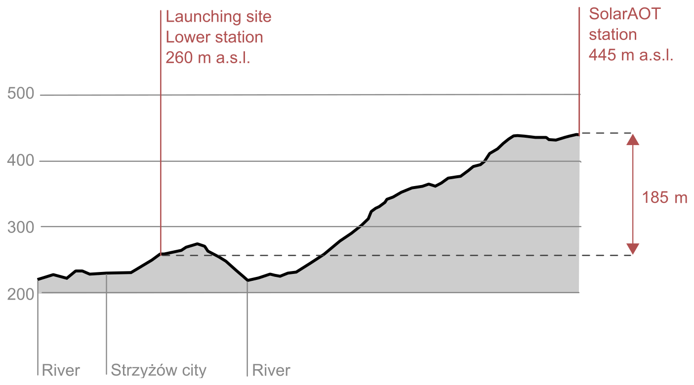
Figure 1 Location of tethered balloon launching site SolarAOT_lower and SolarAOT^upper station, in relation to the city of Strzyżów and the Wisłok River.

A Kipp & Zonen CMP21 pyranometer was used to measure downwelling shortwave radiation (285–2800 nm), including both direct solar and diffuse sky components. For longwave radiation, an Eppley pyrgeometer was employed, operating in the spectral range of approximately 4.5 to 50 µm, to capture downwelling infrared radiation emitted by the atmosphere and clouds. Both sensors were installed on a leveled platform in an unobstructed area.

CIMEL is an instrument for measuring direct and scattered solar radiation in nine spectral channels: 340, 380, 440, 500, 675, 870, 936, 1020, and 1640 nm. Based on the measured values, the optical parameters of the aerosol are determined, including the AOD and the Ångström exponent. The data collected by the instrument is processed within the international AERONET measurement network. Nephelometer Aurora 4000 is used to measure light scattering coefficients on aerosols for wavelengths of 450, 525, and 630 nm in 18 ranges of aerosol scattering angles.

Aethalometer AE-31 is used to measure the concentration of equivalent black carbon (eBC) in the atmosphere and the aerosol absorption coefficient of the aerosol. The measurement is performed at seven wavelengths (370, 470, 520, 590, 660, 880, and 950 nm) using the method of changing the transmission of a quartz filter on which the aerosol is deposited.

2.3 Balloon apparatus

Measurements were conducted using two meteorological balloons (for better buoyancy), each approximately 1.5 m in diameter and filled with helium. The balloons were tethered using the Vaisala TTW111 winch (see Fig. 2a). Around 2 m below the balloon, the apparatus was mounted on the rope holding the balloon. The apparatus used to mount below the balloon was as follows (see Fig. 2b):

• Vaisala radiosonde RS41 – collecting data about pressure (p), temperature (T), and relative humidity (RH);

• GY-63 MS5611 – a high-performance pressure sensor module;

• HYT 939 – additional T and RH sensor;

• the Alphasense OPC-N3 – an optical particle sensor that measures particle counts across size bins ranging from 0.35 to 40 µm, as well as PM_1.0¹, PM_2.5, and PM₁₀ – here, OPC-N3 was used to gather information about fog droplets based on the article (Nurowska et al., 2023), such as liquid water content (LWC), effective radius r_eff, and N_c –

• SENSIRION SPS30 – an optical PM sensor that measures PM_1.0, PM_2.5 PM₄, and PM₁₀ mass concentration;

• TFMini – a visibility sensor;

• AE-51 – a miniature aethalometer for measuring the eBC concentration and the aerosol absorption coefficient at a wavelength of 880 nm.

The OPC-N3, an optical particle counter designed by Alphasense Ltd., utilizes a diode laser emitting light at a wavelength of 658 nm, along with an elliptical mirror that directs the laser beam towards a detector. The airflow, driven perpendicularly to the laser beam by an integrated fan, allows for continuous operation. The OPC-N3 quantifies particle number concentration (N_c) across 24 size bins, covering a diameter range from 0.35 to 40 µm. The onboard algorithm converts N_c measurements into PM₁, PM_2.5, and PM₁₀ values. Detailed specification of the OPC-N3 is available in the work by Hagan and Kroll (2020).

OPC-N3 devices are considered low-cost sensors, which means that two identical units may not yield consistent results due to device-to-device variability. Therefore, cross-calibration between sensors or calibration against a reference-grade instrument is necessary to ensure measurement accuracy. Additionally, individual OPC-N3 units may exhibit signal drift over time, requiring periodic recalibration to maintain data reliability.

For this reason, it was not possible to directly use the calibration parameters provided in Nurowska et al. (2023). Instead, the calibration had to be repeated following the methodology described in that work, to ensure compatibility with the specific sensors used in this study. OPC-N3 was calibrated to the ShadowGraph following Nurowska et al. (2023). Results of N_c, LWC, and r_eff were obtained by taking bins of OPC-N3 measuring particles greater than 1.15 µm (bin 7 of OPC-N3).

The calibration equations used between OPC-N3 and Shadowgraph are as follows:

$$\begin{array}{}\text{(1)}& {\displaystyle }{\mathrm{LWC}}_{\mathrm{ShadowGraph}}=\mathrm{6.15}\cdot {\mathrm{LWC}}_{\text{OPC-N3}}+\mathrm{0.11}\text{(2)}& {\displaystyle }{N_{\mathrm{c}}}_{\mathrm{ShadowGraph}}=\mathrm{4.16}\cdot {N_{\mathrm{c}}}_{\text{OPC-N3}}+\mathrm{32.63}\text{(3)}& {\displaystyle }{r}_{\mathrm{eff}}^{\mathrm{ShadowGraph}}=\mathrm{0.70}\cdot r_{\mathrm{eff}}^{\text{OPC-N3}}+\mathrm{3.81}.\end{array}$$

The OPC-N3 allows calculation of the volume droplet size distribution (vDSD), which can be computed using the following formula:

$$\begin{array}{}\text{(4)}& \mathrm{vDSD}\left(r_{\mathrm{b}}\right)=N_{\mathrm{b}}\cdot (\mathrm{\Delta }{r}_{\mathrm{b}}\cdot V_{\mathrm{b}}{)}^{-\mathrm{1}}\cdot r_{\mathrm{b}}^{\mathrm{3}},\end{array}$$

where N_b is the number of droplets in a bin, V_b is the volume of a bin, Δr_b is the width of the bin, and r_b is the mean bin droplet radius. Although the obtained vDSD was not calibrated against the ShadowGraph, it provides information on which droplet sizes contribute most significantly to the LWC at a given altitude.

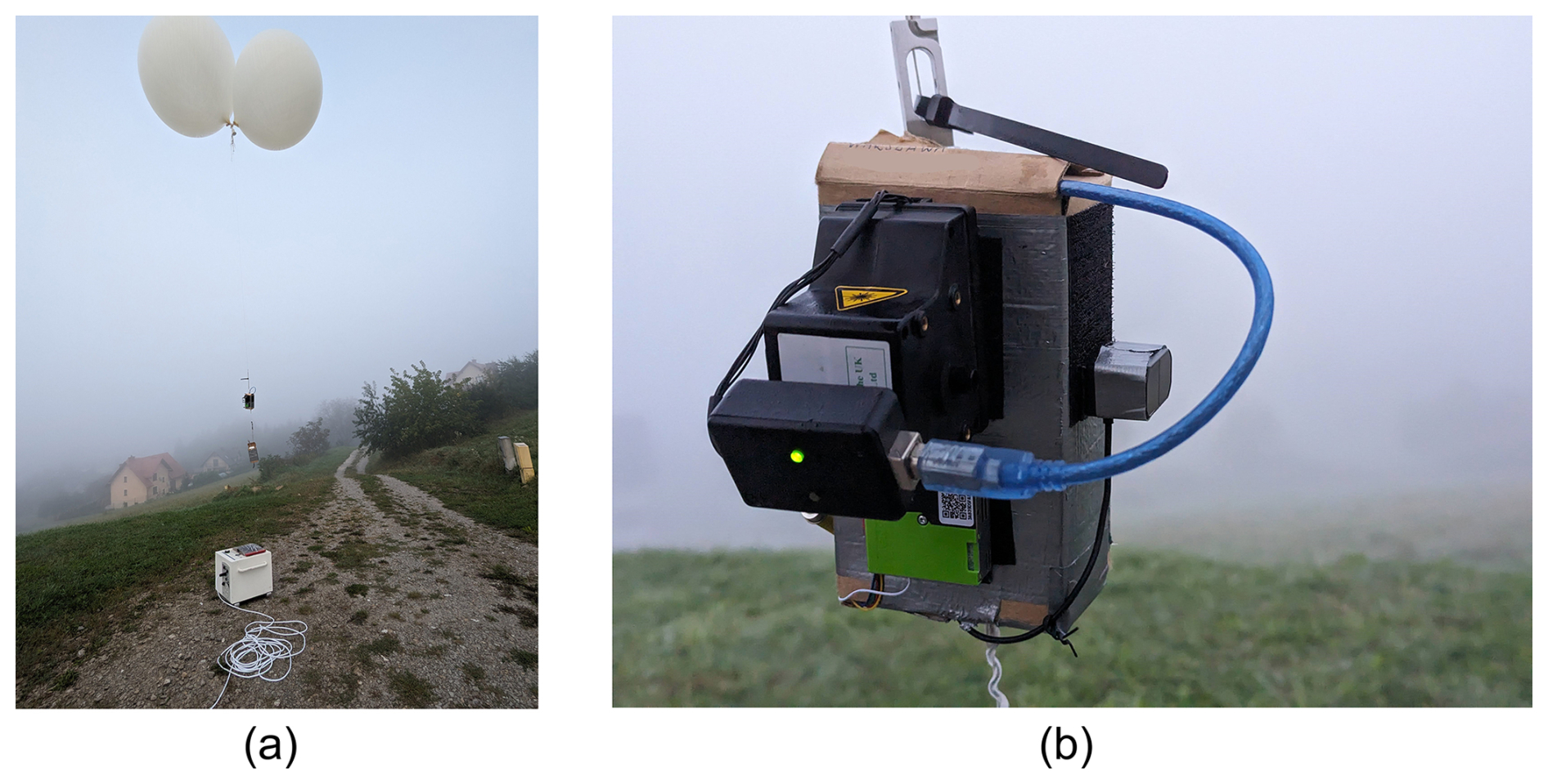
Figure 2 Balloon setup. (a) Balloon with attached payload and connected to the winch. (b) Zoomed-in view of the balloon payload, showing inside the box (GY-63, HYT 939), OPC-N3, SPS30, and TFMini.

3 Methodology and model setup

3.1 Balloon measurement methodology

For 3 d between 9–11 September 2023, the measurements of radiative fog were made in the city of Strzyżów, Poland. The balloon launch site was located in the valley of the city of Strzyżów. Four setups were used, as it was not possible to mount all instruments at once due to the buoyancy:

• setup 1: GY-63, HYT 939, OPC-N3, SPS30, TTFMini – this setup was most common;

• setup 2: only Vaisala radiosonde RS41;

• setup 3: Vaisala radiosonde RS41, AE-51;

• setup 4: Vaisala radiosonde RS41, GY-63, HYT 939, OPC-N3, SPS30, and TFMini.

With colored lines, Fig. 3 shows when, during the night, the soundings were done, with colors indicating different setups mounted on the balloon. The same information, but with specific sounding times, can be found in Appendix B2. In total, 74 soundings were conducted. However, due to data recording issues, 11 soundings lacked complete data and were excluded from further analysis. These are indicated in gray in Fig. 3 and Table B2. Soundings were done by unwinding the rope until it started to tilt to the horizon. The balloon was stopped for a few seconds, and the line was wound up. Soundings were done with around 15 min breaks in between.

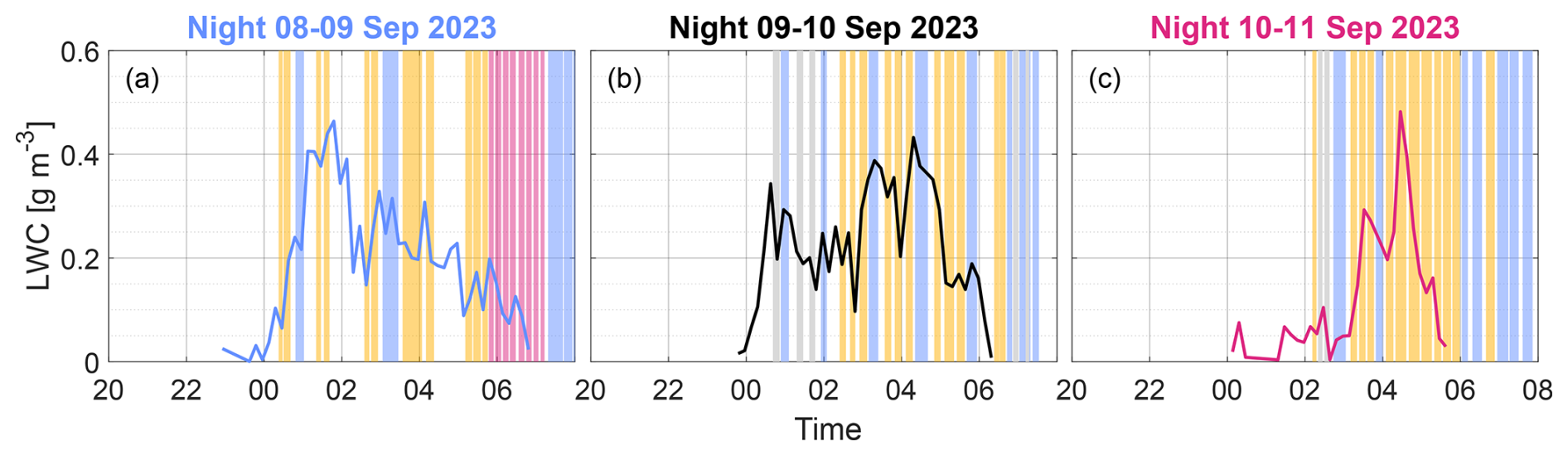
Figure 3 The figure illustrates the timing of the soundings; different colors represent the specific equipment configurations mounted on the balloon: orange – setup with OPC-N3, blue – setup with radiosonde, pink – setup with OPC-N3 and radiosonde, gray – problems with collected data. The image is overlaid on the line representing temporal variability of the LWC at the ground obtained from Shadowgraph (the same data as in Fig. 5).

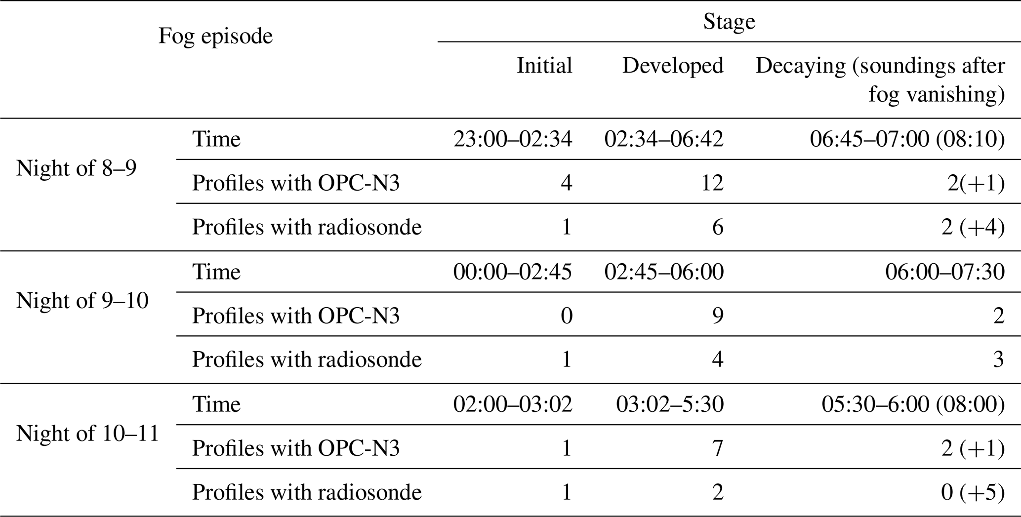
The fog case description was divided into three stages: initial, developed, and decaying. The transition from the initial to the developed stage was assumed to occur when LWP > 15 g m⁻²; the change from mature to decaying was assumed when LWP < 15 g m⁻². Table 1 presents information about each fog stage.

Table 1 Times of initial, developed, and decaying stage of observed fogs on days 9–11 September, with information on how many soundings were performed in each period.

During one balloon launch, we obtained two vertical profiles, which were then averaged over height to obtain a less noisy image due to random fluctuations. All the data were interpolated every 1 m for making figures. On the plots, soundings start at 2 m above ground.

3.2 Adiabatic LWC

Equivalent adiabaticity (α_eq) relates theoretical adiabatic LWC profiles to observed ones. It has been used in studies aiming to estimate cloud base height or improve fog forecasting based on satellite data. For instance, Cermak and Bendix (2011) proposed a model comparing theoretical and satellite-derived LWP to infer cloud base height, while Toledo et al. (2021) applied a similar approach to model fog dissipation. In this section, we present the theoretical derivation of α_eq, which is defined as the scaling factor applied to the adiabatic LWC profile to match the theoretical LWP with the observed value.

To describe the change of LWC in a perfect adiabatic cloud, the following equation is used (Eq. 5) (Cermak and Bendix, 2011; Toledo et al., 2021; Costabloz et al., 2025):

$$\begin{array}{}\text{(5)}& {\displaystyle \frac{\mathrm{dLWC}\left(z\right)}{\mathrm{d}z}}={\mathrm{\Gamma }}_{\mathrm{ad}}\left(T\right(z),p(z\left)\right),\end{array}$$

where z is the height calculated from the base of the cloud. Γ_ad(T(z),p(z)) is the negative of the change in saturation mixing ratio with height for an ideal adiabatic cloud; in other words, it is the adiabatic condensation rate. The processes in stratus clouds are nearly adiabatic; the deviation from adiabatic conditions is introduced into the equation as a parameter α. The fog is similar to stratus cloud; however, to integrate Eq. (5) apart from adding α, non-zero surface liquid water content (LWC₀) must be taken into account.

$$\begin{array}{}\text{(6)}& \begin{array}{rl}\mathrm{LWC}\left(z\right)& =\underset{z^{\prime }=\mathrm{0}}{\overset{z^{\prime }=z}{\int }}\mathit{\alpha }\left(z^{\prime }\right){\mathrm{\Gamma }}_{\mathrm{ad}}\left(T\right(z^{\prime }),p(z^{\prime }\left)\right)\mathrm{d}{z}^{\prime }+{\mathrm{LWC}}_{\mathrm{0}}\\ & \approx {\mathrm{\Gamma }}_{\mathrm{ad}}(T_{\mathrm{B}},p_{\mathrm{B}})\underset{z^{\prime }=\mathrm{0}}{\overset{z^{\prime }=z}{\int }}\mathit{\alpha }\left(z^{\prime }\right)\mathrm{d}{z}^{\prime }+{\mathrm{LWC}}_{\mathrm{0}}\end{array}\end{array}$$

LWP is defined as

$$\begin{array}{}\text{(7)}& \mathrm{LWP}=\underset{z^{\prime }=\mathrm{0}}{\overset{z^{\prime }=\mathrm{CTH}}{\int }}\mathrm{LWC}\left(z^{\prime }\right)\mathrm{d}{z}^{\prime }.\end{array}$$

As fog base is at the ground, the integration takes place from z^′ equal zero to cloud/fog top height (CTH).

In the case of shallow clouds Γ_ad(T(z),p(z)) can be assumed constant with height (Brenguier, 1991); ${\mathrm{\Gamma }}_{\mathrm{ad}}(T_{\mathrm{B}},p_{\mathrm{B}})=$ const., where T_B and p_B are temperature and pressure at fog base/ground, respectively. Since the dependence of α(z) is unknown, the concept of equivalent adiabaticity α_eq= const. is introduced. α_eq is defined as the constant adiabaticity value that would give the same LWP value when replacing α(z^′) in Eq. 6 and calculating LWP from Eq. (7). After taking α_eq= const. the formula for LWP becomes

$$\begin{array}{}\text{(8)}& \mathrm{LWP}={\displaystyle \frac{\mathrm{1}}{\mathrm{2}}}{\mathit{\alpha }}_{\mathrm{eq}}{\mathrm{\Gamma }}_{\mathrm{ad}}(T_{\mathrm{B}},p_{\mathrm{B}})\cdot {\mathrm{CTH}}^{\mathrm{2}}+{\mathrm{LWC}}_{\mathrm{0}}\cdot \mathrm{CTH}.\end{array}$$

The formula for LWC with the above assumptions is

$$\begin{array}{}\text{(9)}& \mathrm{LWC}\left(z\right)={\mathit{\alpha }}_{\mathrm{eq}}{\mathrm{\Gamma }}_{\mathrm{ad}}(T_{\mathrm{B}},p_{\mathrm{B}})\cdot z+{\mathrm{LWC}}_{\mathrm{0}}.\end{array}$$

The method of calculating Γ_ad(T_B,p_B) was taken from Appendix A of the article (Toledo et al., 2021).

To calculate what α_eq, just reverse Eq. (8):

$$\begin{array}{}\text{(10)}& {\mathit{\alpha }}_{\mathrm{eq}}={\displaystyle \frac{\mathrm{2}(\mathrm{LWP}-{\mathrm{LWC}}_{\mathrm{0}}\cdot \mathrm{CTH})}{{\mathrm{\Gamma }}_{\mathrm{ad}}(T_{\mathrm{B}},p_{\mathrm{B}})\cdot {\mathrm{CTH}}^{\mathrm{2}}}}.\end{array}$$

In the literature, instead of α_eq, the parameter β is sometimes used, introduced by Betts (1982) as the in-cloud mixing parameter. This parameter measures departure from the adiabatic situation. The relation between α_eq and β is ${\mathit{\alpha }}_{\mathrm{eq}}=\mathrm{1}-\mathit{\beta }$.

In the latter part of this article, the following will be used:

• Γ_ad – adiabatic condensation rate of LWC;

• α_eq – scaling of Γ_ad, which would give the same LWP for the whole cloud/fog;

• α_fit – scaling of Γ_ad obtained by fitting line to LWC dependence from height;

• Γ_wa – moist adiabatic lapse rate for T;

• γ_fit – scaling of Γ_wa obtained by fitting line to T dependence from height.

Figure 4 presents the visualization of the concepts listed above.

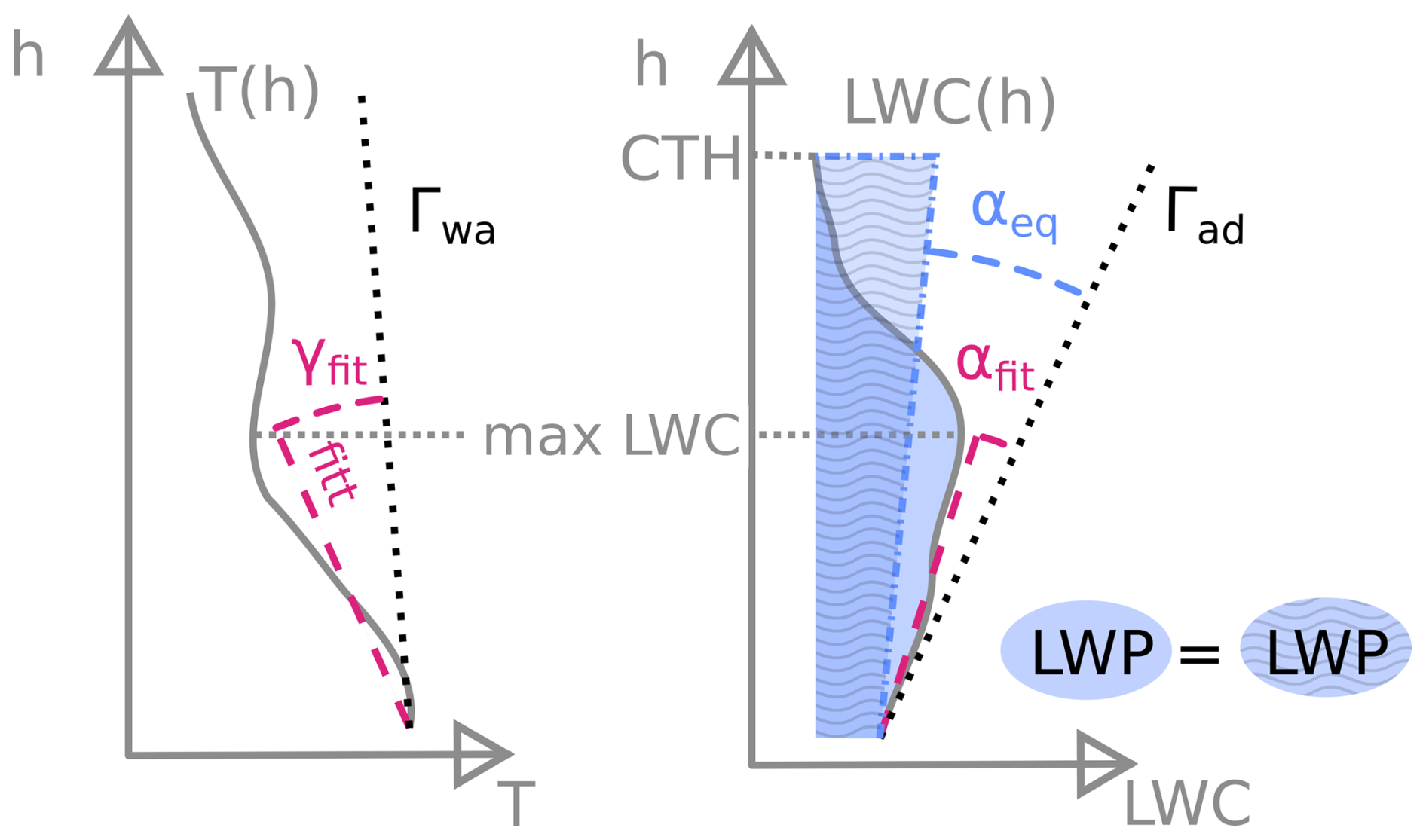
Figure 4 Representation of profile of T and LWC with added lines of Γ_wa and Γ_ad respectively. γ_fit and α_fit represents the angle between the best line fit to T and LWC, respectively (from bottom to height of max LWC), and Γ_wa and Γ_ad. α_eq= const. is defined as deviation from Γ_ad, which would give the same LWP as the original data.

3.3 Radiometer data processing

At the SolarAOT^upper station, a CMP21 pyranometer and an Eppley pyrgeometer were installed to measure downwelling shortwave and longwave radiation, respectively. Both instruments recorded data at 42 s intervals. At the SolarAOT_lower station, a CNR4 net radiometer was mounted to measure both upward and downward shortwave and longwave fluxes, with a sampling interval of 36 s. Data from SolarAOT^upper were interpolated to match the temporal resolution of the lower station. Short spikes in the radiometric signal – likely due to transient obstructions such as birds – were removed using a filtering algorithm. Additionally, the signal was smoothed using a 10 min running mean. The 10 min averaging window was chosen to correspond to the typical duration of balloon flights (10–15 min), allowing for comparison between the measured and simulated radiative fluxes.

3.4 1D simulation radiation fluxes

This section presents the model used to perform optical, microphysical, and radiative closure, as discussed in Sect. 4.4. The model was used to assess the consistency between observed radiation and retrieved fog microphysical properties. For this purpose, simulations were done in 1D using the Fu–Liou code (Fu and Liou, 1992, 1993).

The Fu–Liou radiative transfer model is a sophisticated tool designed to accurately simulate radiative transfer in the Earth's atmosphere. The Fu–Liou code uses δ-four-stream and δ-two-stream flux approximation, which allows it to efficiently handle the complexities of radiation scattering and absorption by gases, aerosols, and cloud particles. The model covers 6 shortwave (SW, λ< 4 µm) and 12 longwave (LW, λ≥4 µm) spectral bands, making it well suited for various atmospheric conditions. The Fu–Liou model provides detailed insights into the interactions between cloud microphysics and radiation. The model vertical levels span the ground up to 10 km, with a greater density closer to the surface. In the first 100 m, the grid was spaced every 10 m and from 100 m to 1 km every 100 m. Input into the Fu–Liou model includes profiles of thermodynamic parameters, fog optical and microphysical quantities, aerosol optical properties, and surface reflectance and emissivity.

To perform simulations, the following specific data were provided to the model:

• T and specific humidity profile. The data from the soundings were combined with the sounding from Tarnów (WMO station 12575) – more information is given in Appendix A.

• r_eff. Due to limitations of the radiative transfer model, r_eff was assumed to be constant with height within the fog layer. It was calculated using data from the OPC-N3, which measures droplet concentrations in 24 size bins. To exclude aerosol particles, only bins 7 to 24 (corresponding to droplet diameters from 1.15 to 20 µm) were used in the calculation.

• Fog height. In the model it was assumed that the fog starts at the surface and reaches the CTH level. The top of the fog was determined as the point where LWC < 0.12 g m⁻³.

• Aerosol optical depth (AOD). Measurements from CIMEL at SolarAOT^upper were taken. To adjust how much the beam is weakened by the vertical distance between the upper and lower site, the value of AOD was added to the extinction coefficient (obtained from Aurora 4000 and AE-31) times the height difference (185 m) between both stations.

• Aerosol single scattering albedo (SSA). Based on AE-31 and Aurora 4000 located at SolarAOT^upper, the SSA was calculated. The value of SSA at the moment of the balloon sounding was obtained by linear interpolation.

• Aerosol Ångström exponent (AE) at 440/870 nm. A CIMEL sun photometer is installed at the SolarAOT^upper site. For the simulations, AE values were rounded to ensure consistent conditions across all cases. Data from both CIMEL and lidar indicate an influx of Saharan dust during the period of 8–10 September. The approximate AE value recorded by CIMEL during these days was 0.5, increasing to 1.0 on 11 September.

• The asymmetry parameter was derived using Mie scattering theory. Initially, the liquid water content and effective droplet radius were employed to estimate the droplet number concentration, assuming a monodisperse size distribution. Subsequently, spectral optical properties – extinction, scattering, and single scattering albedo – were computed across relevant wavelengths. Finally, the asymmetry parameter was calculated by integrating the angular scattering phase function obtained from classical Mie theory.

• The model allows for the specification of surface albedo based on the International Geosphere-Biosphere Program (IGBP) land cover classification, using one of 20 predefined surface types. For all simulations performed in this study, the IGBP class was set to “grassland” (IGBP = 10), as the measurement site was located on a valley slope predominantly covered with grass, with sparse one-family houses. Surface albedo was implemented as a spectrally resolved, solar zenith, and water-vapor-content-dependent parameter.

4 Case study: valley of the city of Strzyżów

Fog was observed during three successive nights between 8 and 11 September 2023 in the valley of the city of Strzyżów. The balloon was launched after fog was visible at the lower station. Figure 5 presents the situation at the lower and upper stations during fog occurrence. Figure B2 presents photographs taken on 3 consecutive days at 04:00 UTC (all times in the paper are given in UTC unless specified otherwise) from the SolarAOT^upper station, showing the top of the fog layer. During the experiment, the fog was not detected at the upper site. Table 1 presents the duration of each fog event and its division into stages. In this section the evolution of each fog event will be described as well as its general pattern. The analyzed data are available for download from the Dane Badawcze UW repository (Nurowska, 2025).

4.1 Meteorological overview

The area of Poland, as well as almost all of Europe, was under the influence of anticyclonic circulation of high pressure from Russia. The pressure on 9 September was constant at 1019 hPa; from 09:00 UTC on 10 September it began to slowly drop to reach the value of 1012 hPa on 11 September at 11:00 UTC. During 8–10 September 2023, there was an event of Saharan dust over Poland. The AE measured for those days by CIMEL at SolarAOT^upper station was around 0.5 (for a period of Saharan dust) and 1.0 (for the morning of 11 September). The mean AOD during the dust episode was not very high (0.19 at 500 nm). It can be seen from the lidar data (Fig. B1) that the sky was mostly cloudless. On 9 September in the morning, cirrus clouds were visible. The average wind speed did not exceed 2.5 m s⁻¹. Slow advection of hot air of tropical origin caused an inflow of Saharan mineral dust visible at 2–4 km a.g.l. on lidar data (Fig. B1). Figure 5d shows the aerosol scattering coefficient of light at 525 nm (ASC₅₂₅), for 3 nights of observations. On the night between 8–9 September 2023 ASC₅₂₅ was below 100 Mm⁻¹, which suggests moderate air quality conditions; just before the onset of fog at 21:30–22:30, the values peak to 240 Mm⁻¹, and after the end of fog, values once again peak exceed a very high level of 500 Mm⁻¹. These two peaks are probably due to industrial activity during inversion conditions and the turning on of the heating systems in houses. The morning peak is coincident with inversion disappearance and the transport of pollution from the bottom of the Strzyżów valley. On the night between 9 and 10 September ASC₅₂₅ descended during the night from 150 to 100 Mm⁻¹, with a peak to 250 Mm⁻¹ at 21:00 UTC. The cleanest conditions, with no evening peak of ASC₅₂₅, were on the night of 11 September, with values below 100 Mm⁻¹. At the upper station, always in the evening and at night, the values of ASC₅₂₅ were below 100 Mm⁻¹. The air in the valley was trapped under the inversion of temperature. The inversion formed at 18:00 at night from days 8 and 9 and around 19:00 at night on 10 September 2023. The course of T in the valley each day was similar during the day, reaching a maximum of 24–26 °C and reaching a minimum 12.5–13.5 °C around 05:00 UTC (Fig. 5). The inversion disappeared around 08:40, 07:40, and 08:10, respectively, for days 9, 10, and 11 September 2023. The RH at SolarAOT_lower station during fog reached 100 %. The air at SolarAOT^upper station was lower (RH = 60 %–90 %).

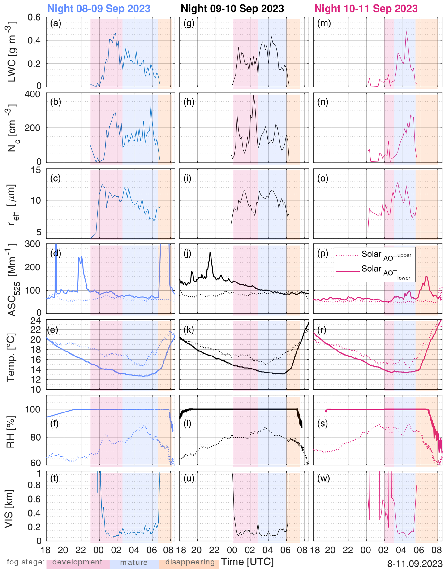
Figure 5 Temporal variability of weather condition on the ground for 9, 10, and 11 September 2023 at the SolarAOT_lower site (solid lines) and SolarAOT^upper station (dotted line). In panels (a), (g), and (m) LWC from ShadowGraph is presented; for reference, when the soundings of the balloon with installed OPC-N3 occurred, an overlay of Fig. 6 was added. Panels (b), (h), and (n) present the N_c of droplets registered by ShadowGraph. Panels (c), (i), and (o) show r_eff obtained from ShadowGraph. Panels (d), (j), and (p) present the ASC at 525 nm from Aurora 4000; panels (e), (k), and (r) T; panels (f), (l), and (s) RH; and panels (t), (u), and (w) visibility obtained from ShadowGraph.

The lower panels of Fig. 5 show the calculated visibility in kilometers. Visibility was derived from ShadowGraph measurements using the Koschmieder formula, under the assumption of monodisperse droplets with a radius equal to the r_eff obtained from ShadowGraph, and LWC also provided by ShadowGraph data. An extinction coefficient of 2 was assumed, corresponding to the geometrical optics regime.

During the nights of 9 and 10 September, visibility decreased sharply around midnight, reaching values as low as 100–200 m. The fog dissipated abruptly around 06:00. In contrast, the fog event on the night of 11 September exhibited a different evolution: intermittent patches of fog began to form around midnight, followed by the development of a more continuous fog layer after 02:00, which persisted until approximately 06:00.

4.2 Fog microphysics

Based on OPC-N3 measurements, it was possible to compute LWC and LWP; results for each fog event are presented in Fig. 6. Observed fog mostly occurred in moderate aerosol conditions, and fog layers were located in the range of the T inversion. The fog top varied from sounding to sounding; mostly it was 85 m (max. 115 m, see Fig 6).

.

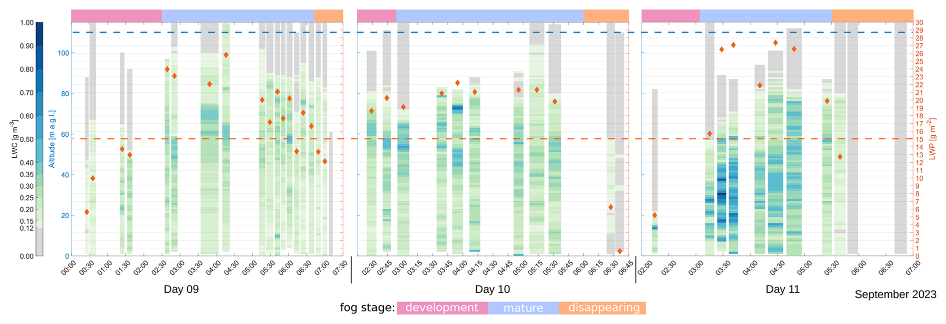
Figure 6 The bar chart with green–blue colors indicates the change in time of fog LWC with height for days (a) 9, (b) 10, and (c) 11 September 2023. The left axis represents the height, while the right axis corresponds to the total LWP for each balloon sounding (marked by an orange diamond). Blue dashed line indicates the 110 m, and orange line indicates LWP equal to 15 g m⁻². These are criteria indicating the transition from thin to thick fog by Costabloz et al. (2025)

Figures 7, 8, and 9 present the T and RH with height as well as LWC, N_c, and r_eff for each fog event. The profiles are shown starting from 2 m above the ground, as values below this height could have been significantly affected by surface influence or local disturbances during balloon launch procedures. For this reason, the lines fitted to the profiles were calculated from 2 m to 80 % of the fog height. The level of 80% was chosen according to Cermak and Bendix (2011), that above 80 % of the height, the fog layer mixes with the dry air above it, which contributes to the reduction of LWC. It is worth mentioning that at that stage of the year, the sunrise is at 04:00 UTC (local time 06:00). Time is given in UTC; for this period of year, UTC is −2 h from local time.

4.2.1 Thin-to-thick transition

In the observed fog events, several criteria were considered to identify a possible transition from thin to thick fog. Following Costabloz et al. (2025), we evaluated: IR net radiation at the surface, temperature, cloud top height, and liquid water path.

Costabloz et al. (2025) proposed five conditions to characterize this transition: (1) longwave net radiation approaches zero, (2) the temperature gradient between 50 and 25 m becomes negative, (3) TKE exceeds 0.10 m² s⁻², (4) CTH exceeds 110 m, and (5) LWP exceeds 15 g m⁻². They demonstrated that while all conditions were met for thick fog, the exact time when each was fulfilled could differ by up to 1 h, making precise estimation of the transition time challenging. In this study, we evaluated four out of five conditions proposed by Costabloz et al. (2025) (without the TKE condition). The following list outlines which criteria were met during each observed fog event.

• On the night of 8–9 September, the LWP exceeded 15 g m⁻² at 01:30. The IR net radiation criterion was satisfied for three profiles at 02:38, 03:48, and 04:16. The profile at 04:16 satisfied three out of the four criteria (IR net radiation, CTH, and LWP) and was conducted during a brief period of thicker fog just before sunrise. However, this state of thick fog did not persist for long.

• On the night of 9–10 September, the LWP exceeded 15 g m⁻² from the start of valid measurements at 02:30 until the fog dissipated.

• On the night of 10–11 September, the LWP exceeded 15 g m⁻² at 03:10, but the CTH did not reach the 110 m threshold.

Although the 15 g m⁻² threshold suggested by Costabloz et al. (2025) was frequently exceeded, our results indicate that this value alone is insufficient to reliably distinguish between thin and thick fog. Therefore, we interpret the fog event on 9 September as a case in which a transition towards thick fog had started but was interrupted by sunrise before full development. In the fog events on 10 and 11 September, the other criteria were not met. In none of these cases did the LWP exceed 30 g m⁻² – the threshold for thick fog proposed by Wærsted et al. (2017). Given that the period of thick fog was very short-lived and most observations remained within the thin fog regime, our findings should be considered primarily representative of optically thin fog conditions.

4.2.2 Night of 8–9 September 2023

The fog event during the night of 8–9 September 2023 was observed from its development stage (23:00–01:41) through its mature stage (02:45–06:42) until dissipation (06:45–07:00). Figure 7 presents vertical profiles of microphysical parameters, including LWC, N_c, and r_eff, along with T and RH. The equivalent adiabaticity (α_eq) is shown in the figures displaying LWC profiles. The division into fog life cycle stages is illustrated in Fig. 7 by pink, blue, and yellow ochre corresponding to the development, mature, and dissipation stages, respectively. Apart from that, separate figures can be found in the Appendix for each stage: Figs. B3a and b and  B4. Each of the fog stages is described below.

• Development of fog. There were five soundings conducted between 23:00–02:34 (see Fig. B3a). T decreased with height from the ground to 40 m a.g.l., starting from T= 12.0 °C and decreasing at the rate ${\mathit{\gamma }}_{\mathrm{fit}}\cdot {\mathrm{\Gamma }}_{\mathrm{wa}}=\mathrm{0.48}\cdot (-\mathrm{5.0})$ °C km⁻¹. Above 40 m, a temperature inversion was present, with T reaching 14.7 °C at 100 m. The top of the fog was 65 m. The RH was constant, equal to 100 % up to 87 m, and in the last 10 m it dropped with height (96 % at 100 m). LWC slightly increased with height (${\mathit{\alpha }}_{\mathrm{fit}}\cdot {\mathrm{\Gamma }}_{\mathrm{ad}}=\mathrm{1.34}\cdot \mathrm{2.32}$ g m⁻³ km⁻¹), from 0.18 to a maximum of 0.30 g m⁻³ at 23 m a.g.l.; up to 36 m a.g.l., LWC was oscillating near 0.26 g m⁻³, and above that it decreased. α_eq was 0.29. LWC_ShadowGraph (referring to LWC measured by the ShadowGraph, Fig. 5) shows that during the development stage, LWC_ShadowGraph increased, reaching its maximum of 0.46 g m⁻³ at 01:47. Values of LWC from ShadowGraph were higher than those from OPC-N3. LWP (Fig. 6) increased from 5.63 g m⁻² at 00:25 to 12.97 g m⁻² at 01:36. Mean N_c increased with height to 247 cm⁻³ at 35 m and then decreased with height to 48 cm⁻³ at 65 m. r_eff decreased steadily with height from 11.2 to 5.7 µm at the CTH.

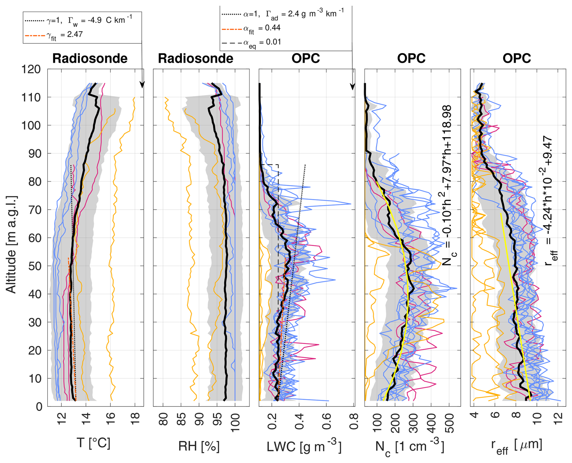
• Mature state of fog. There were 13 soundings conducted from 02:34 till 06:42 (Fig. B3b). T and RH showed a similar pattern to height, as in the previous stage. The fog was deeper, with a top at 102 m. However, the temperature inversion started higher, around 60 m above the ground, and the lapse rate in the lower part was higher: ${\mathit{\gamma }}_{\mathrm{fit}}\cdot {\mathrm{\Gamma }}_{\mathrm{wa}}=\mathrm{1.16}\cdot (-\mathrm{5.1})$ °C km⁻¹. The N_c maximum, equal to 410 cm⁻³, was at 48 m; above this, N_c decreased to 65 cm⁻³ at 90 m. Above that, the number of drops was constant. The r_eff profile changed and can be divided into two sections. From the ground to a height of 88 m, r_eff remained almost constant (at bottom 9.2 µm; 8.3 µm at 88 m). From 88 m to CTH, r_eff decreased sharply with height (mean at the top 5.2 µm). Because the N_c maximum is shifted upward, the LWC maximum is also at a higher altitude (56 m). The α_fit is positive, equal to 0.90, and α_eq is equal to 0.30. The images from the ShadowGraph indicate that LWC_ShadowGraph near the ground decreased over time starting from 2:57, and this was associated with a decrease in r_eff and not N_c.

• Disappearing stage. There were two soundings conducted between 06:45 and 07:00 (Fig. B4). T increased from the ground to 27 m, above which T decreased with height. Unfortunately, the sounding with the Vaisala radiosonde RS41 was interrupted at 45 m. Between the two soundings, spaced less than 15 min apart, the T profile shifted by +2 °C. At this time, the RH profile dropped by 5 %. In the first 20 m, the mean RH dropped from 96 % near the ground to 91 % at 20 m. The fog evaporated quickly. The α_eq was positive, equal to 0.33. LWC increased with height (${\mathit{\alpha }}_{\mathrm{fit}}\cdot {\mathrm{\Gamma }}_{\mathrm{ad}}=\mathrm{0.42}\cdot \mathrm{2.39}$ g m⁻³ km⁻¹), reaching a maximum at 72 m (mean LWC 0.26 g m⁻³); at almost the same height, N_c also reached its maximum (488 cm⁻³ at 74 m). The layer above was characterized by a rapid decrease in both values up to the CTH. The r_eff was constant with height up to 80 m, around 6.8 µm, except for the layer from the ground to 18 m, where r_eff was higher, up to 9.5 µm.

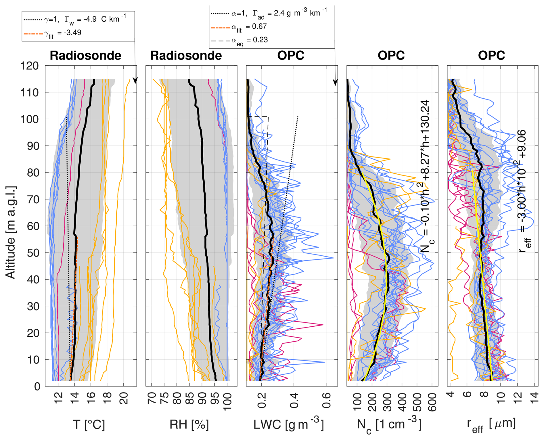
Figure 7 Vertical profiles of specific quantities measured by the balloon for the night of 8–9 September 2023. From left: T and RH from Vaisala radiosonde RS41, LWC, N_c, and r_eff within the fog from OPC-N3. Each colored line represents an individual balloon profile, with different colors indicating different stages of fog evolution: pink corresponds to the formation stage, blue to the mature stage, and yellow ochre to the dissipation stage. The black thick line represents the mean of all the soundings, and the colored area represents the range between ± standard deviation from the mean. In the T plot, the dotted line presents the wet adiabatic lapse rate Γ_w, and the dashed red line presents linear fit of T from 2 m to height of maximum mean LWC. γ_fit is a scaling factor of Γ_w to obtain the equation of linear fit. In the LWC plot, the dotted line presents the LWC adiabatic lapse rate Γ_ad, and the dashed red line presents the linear fit to LWC from 2 m to the height of maximum mean LWC. α_fit is a scaling factor of Γ_ad obtained by fitting line to LWC dependence from height, and α_eq is a scaling of Γ_ad, which would give the same LWP for the whole cloud/fog. In the N_c plot, the yellow line indicates the quadratic fit to the data (from 2 m to 80 % height of CTH). In the r_eff plot, the yellow line indicates the linear fit to the data (from 2 m to 80 % height of CTH).

Figure 7 presents the mean values with height for the whole-night fog event from 8–9 September 2023. For the entire fog event, α_eq is 0.23. As a first approximation, fog r_eff decreases linearly with height, while N_c can be approximated by a quadratic equation. The equations for fitted lines are, respectively,

$$\begin{array}{}\text{(11)}& {\displaystyle }{r}_{\mathrm{eff}}=\mathrm{0.03}\cdot h+\mathrm{9.06}\left[\mathrm{\mu }\mathrm{m}\right],\text{(12)}& {\displaystyle }{N}_{\mathrm{c}}=-\mathrm{0.10}\cdot h^{\mathrm{2}}\cdot \mathrm{10}+\mathrm{8.27}\cdot h+\mathrm{130.24}\left[{\mathrm{cm}}^{-\mathrm{3}}\right].\end{array}$$

Figure 8 Vertical profiles of specific quantities measured by the balloon for the night of 9–10 September 2023. A detailed description is given in the caption of Fig. 7.

4.2.3 Night of 9–10 September 2023

Below are described the stages of fog from 9–10 September 2023:

• Development of fog. Due to a malfunction of the apparatus, the development stage of fog with microphysics measurements in the vertical direction was not captured. The fog started at 00:00; however, it is not possible to determine when this stage ended. The first OPC-N3 sounding was registered at 02:34, with LWP > 15 g m⁻².

  Based on ShadowGraph measurements, LWC and N_c increased continuously until 00:37, reaching local maxima: LWC_ShadowGraph= 0.34 g m⁻³ and N_c= 271 cm⁻³. The r_eff reached its local maximum later, at 01:17, equal to 11.6 µm. After the peak, values of LWC, N_c, and r_eff fluctuated, reaching their global maxima (N_c= 388 cm⁻³ at 02:18) and minima (r_eff= 7.5 µm at 02:28).

  Two profiles of T and RH are shown in Fig. B5a. The profile reaching a higher altitude was performed earlier, at 00:53, and the second about 1 h later. The temperature profile was nearly constant in the first 40 m (12.65 °C at the ground), above which a temperature inversion was present that weakened with time. The RH was 100 % up to 67 m and then decreased with height. RH was constant at 100 % throughout the entire column from the ground up to 86 m 1 h later.

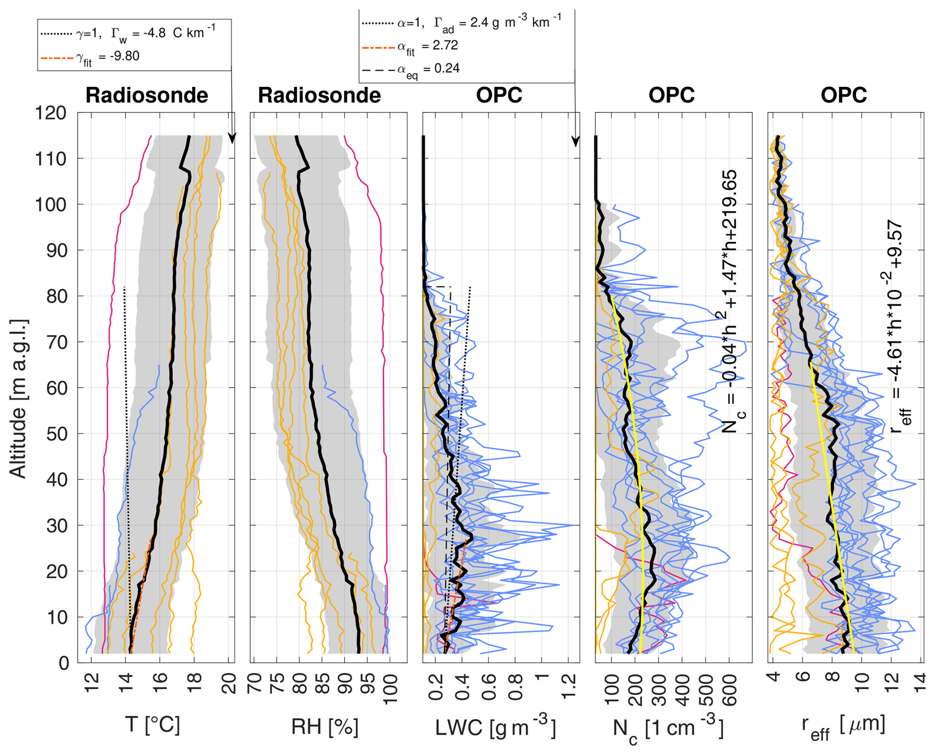
• Mature state of fog. There were 13 soundings conducted from 02:45 to 06:42 (Fig. B5b). The fog height was 87 m. The temperature decreased with height up to 50 m a.g.l., above which a temperature inversion occurred. From the ground to the CTH, RH remained above 99.5 %. The maximum LWC was observed at 53 m, with a value of 0.40 g m⁻³.

  A linear fit to the LWC profile from 2 to 53 m yielded a growth rate equal to 0.51 of the LWC adiabatic lapse rate. The maximum N_c was lower than during the previous night, reaching 345 cm⁻³. The r_eff at the ground was higher than in the previous day's fog; however, it decreased with height in the first 30 m, remained approximately constant (9.0 µm) from 30 to 63 m, and then decreased again toward the CTH.

  The LWP (Fig. 6) oscillated between 18 and 23 g m⁻². Most of the water was located in the upper part of the fog, between 30 and 70 m.

• Disappearing stage. Five soundings were conducted between 06:30 and 07:30 (Fig. B6). The temperature at 2 m a.g.l. and throughout the column increased rapidly (from 11.9 °C at 06:30 to 16.22 °C at 07:30). In the first 54 m, T decreased with height, and above this level, a temperature inversion was observed. As the sun rose, RH decreased from 100 % to 88 % at 2 m a.g.l.

  The parameters α_fit and α_eq were 0.30 and 0.24, respectively. LWC values were below 0.12 g m⁻³ in the first 21 m above the ground. The maximum LWC (0.15 g m⁻³) occurred at 43 m. When fog almost dissipated (06:23; Fig. 6), remaining fog patches were still observed between 30 and 50 m, with LWC > 0.15 g m⁻³. The fog top dropped to 57 m.

  Fog droplet diameter decreased with height from 6.7 µm at 4 m a.g.l. to 4.8 µm at the CTH. N_c fluctuated around 170 cm⁻³ between 24 and 56 m. The fog dissipated from both the top and bottom.

The temperature in the first 53 m was almost constant with height. Within this layer, LWC increased with height at a rate of ${\mathit{\alpha }}_{\mathrm{fit}}\cdot {\mathrm{\Gamma }}_{\mathrm{ad}}=\mathrm{0.44}\cdot \mathrm{2.4}$ g m⁻³ km⁻¹, reaching a local maximum of LWC = 0.33 g m⁻³ at 53 m. The corresponding value of α_eq was nearly zero (0.01).

Figure 8 summarizes the microphysical properties of the fog event on 9–10 September 2023. The following curves were fitted to the values of N_c and r_eff:

$$\begin{array}{}\text{(13)}& {\displaystyle }{N}_{\mathrm{c}}=-\mathrm{0.10}\cdot h^{\mathrm{2}}\cdot \mathrm{10}+\mathrm{7.97}\cdot h+\mathrm{118.98}\left[{\mathrm{cm}}^{-\mathrm{3}}\right],\text{(14)}& {\displaystyle }{r}_{\mathrm{eff}}=\mathrm{4.29}\cdot h\cdot {\mathrm{10}}^{-\mathrm{2}}+\mathrm{9.47}\left[\mathrm{\mu }\mathrm{m}\right].\end{array}$$

4.2.4 Night of 10–11 September 2023

The fog pattern on the night of 10–11 September looks distinct from previous nights. The fog could not form until 03:08, when it started to develop with an abrupt jump in LWC from 0.05 at 03:08 to 0.30 at 03:31. The maximum peak in LWC observed on the ground by ShadowGraph was at 04:27, equal to 0.48 g m⁻³. Fog rapidly intensified, reaching high LWC values (mean 0.48 g m⁻³) in the fog body from 10–50 m, with maximum LWC 0.97 g m⁻³ at 31 m at 03:23. At 04:40, high values of LWC above 0.40 g m⁻³ were distributed in the range from the fog bottom to 80 m. As quickly as it appeared, the fog dissipated by 05:40. However, as before, the fog dissipated more from the bottom than from the top.

During the night of 10–11 September 2023, all stages of fog were captured; each stage is described in detail below. This fog event developed later in the night than previous cases and exhibited more abrupt behavior.

• Development of fog. Between midnight and 02:28, the ShadowGraph detected droplets; however, the LWC_ShadowGraph was below 0.1 g m⁻³. Two soundings were performed, one with OPC-N3 and one with the Vaisala radiosonde RS41, between 02:00 and 03:02 (Fig. B7a). The profile from 02:11 shows that the fog was just forming. LWP was 5.23 g m⁻².

  Fog was confined to the first 23 m in height. Even though the fog was shallow, it had high LWC values at some levels (max. LWC was 0.67 g m⁻³ at 13 m). The ${\mathit{\alpha }}_{\mathrm{eq}}=-\mathrm{3.22}$; however ${\mathit{\alpha }}_{\mathrm{fit}}=-\mathrm{0.15}$.

  The fog was dense; the maximum N_c was 416 cm⁻³ at 18 m. The r_eff decreased with height (9.8 µm at 2 m and 6.0 µm at the CTH). The profile from the Vaisala radiosonde RS41 at 02:43 shows that T remained almost constant in the first 40 m (around 12.7–12.8 °C), later slightly increasing with height to 14.2 °C at 100 m.

  The RH profile was constant with height; however, the air was not fully saturated (RH ≈ 98.5 %). ShadowGraph shows that LWC dropped to 0 at 02:38 and within the next hour rapidly rebuilt to 0.30 g m⁻³. This was correlated with rapid growth of r_eff from 7.8 µm to 12.8 µm, while N_c remained low (2–65 cm⁻³).

• Mature state of fog. Between 03:10 and 05:30, eight soundings with a balloon (Fig. B7b) were conducted. The fog deepened to 83 m. The profiles of T and RH changed: only in the first 10 m was RH above 99.5%, above which it decreased to 85.5 % at 60 m.

  Unfortunately, the sounding with the Vaisala radiosonde RS41 did not reach the CTH. There was a strong inversion; the fitted lapse rate was ${\mathit{\gamma }}_{\mathrm{fit}}\cdot {\mathrm{\Gamma }}_{\mathrm{wa}}=-\mathrm{11.82}\cdot -\mathrm{4.97}$ °C km⁻¹. T increased from 12.3 °C at the ground to 15.8 °C at 60 m.

  The N_c profile had a different form compared to previous fog events: it exhibited two protrusions with maxima at 25 m (377 cm⁻³) and 70 m (257 cm⁻³) and a local minimum at 50 m. The r_eff slightly decreased from the ground (10.0 µm) to 60 m (8.8 µm) and then decreased more sharply to 5.5 µm at the CTH.

  The LWC profile showed a more intermittent pattern, with values fluctuating between 0.2 and 1.2 g m⁻³ and a peak of 0.67 g m⁻³ at 27 m. α_eq=0.56, and fitted α_fit=4.80. The LWP was the highest of all three events; for four soundings, LWP exceeded 26.5 g m⁻² (maximum: 27.36 g m⁻² at 04:27).

• Disappearing stage. The final stage of fog was observed from 05:30 to 06:00. Two soundings were conducted with OPC-N3. In Fig. B8, two additional soundings of T and RH between 06:00 and 06:33 are also shown. The CTH was at 79 m.

  LWC increased with height, with a maximum near the CTH (max. LWC = 0.19 g m⁻³ at 75 m). Due to the location of the maximum LWC near the CTH, α_eq=0.32, which was similar to α_fit=0.30.

  N_c increased with height to 27 m (maximum 190 cm⁻³), then oscillated around 145 cm⁻³ up to 43 m, and then sharply decreased to 62 cm⁻³ at 48 m. The r_eff slightly decreased with height, with fluctuations around 6 µm.

Figure 9 summarizes the microphysical properties of the fog event on 10–11 September 2023. α_eq for the entire event was 0.24. The following curves were fitted to the values of N_c and r_eff:

$$\begin{array}{}\text{(15)}& {\displaystyle }{N}_{\mathrm{c}}=-\mathrm{0.04}\cdot h^{\mathrm{2}}+\mathrm{1.47}\cdot h+\mathrm{219.65}\left[{\mathrm{cm}}^{-\mathrm{3}}\right],\text{(16)}& {\displaystyle }{r}_{\mathrm{eff}}=\mathrm{4.61}\cdot h\cdot {\mathrm{10}}^{-\mathrm{2}}+\mathrm{9.57}\left[\mathrm{\mu }\mathrm{m}\right].\end{array}$$

Figure 9 Vertical profiles of specific quantities measured by the balloon for the night of 10–11 September 2023. A detailed description is given in the caption of Fig. 7.

4.3 Evolution of fog droplet spectrum

From the OPC-N3 measurements, it was possible to compute vDSD(r) presented in Fig. 11a. vDSD is presented from bins of radius from 1.15 to 20 µm to remove aerosol particles. ShadowGraph was located near the ground; Fig. 10 presents the comparison between the vDSD obtained from ShadowGraph and OPC-N3. ShadowGraph shows that near the ground, there are droplets of radius greater than 20 µm and that in the case of OPC-N3, those droplets are counted in the last bin. As was stated by Nurowska et al. (2023), even though the manufacturer declares that the upper limit of the last bin is 20 µm, in fact, the last bin also counts larger particles.

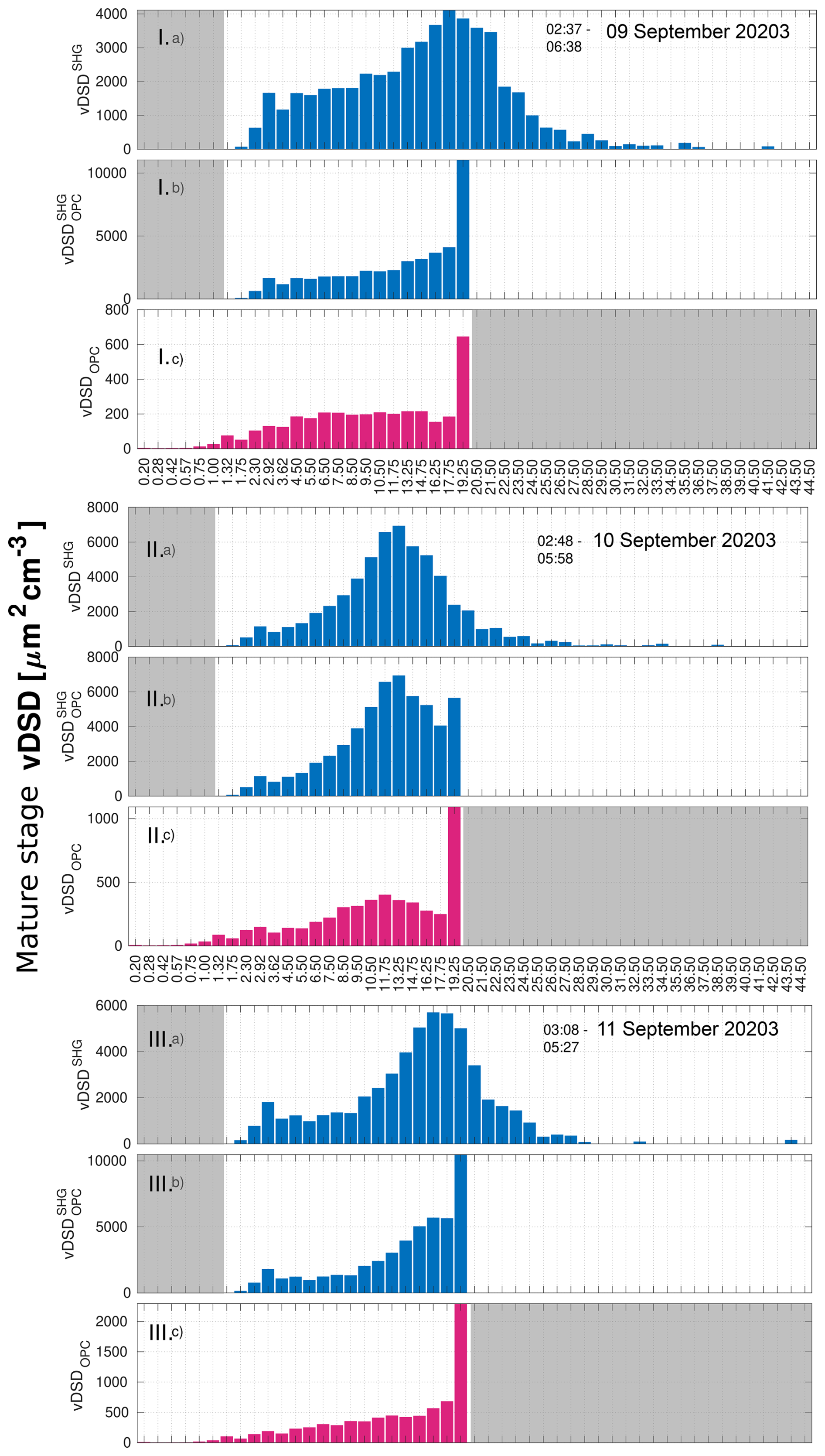
Figure 10 vDSD near ground for mature stage of night events of fog on (I) 8–9 September, (II) 9–10 September, and (III) 10-11 September 2023. Panels (a) and (b) present the vDSD obtained from Shadowgraph, while (c) presents vDSD from OPC-N3. The x axis represents the edges of the bins of droplet radii measured by OPC-N3 and additionally greater bins (above 20 µm) visible only by Shadowgraph. Panel (b) presents the same vDSD as panel (a); however all the droplets with radius greater than 20 µm are counted as part of the last bin of OPC-N3 (18.5–20 µm) – this is done to be able to compare the vDSD from OPC-N3 and Shadowgraph. The imaging area for a given device is marked in white.

Although OPC-N3 is not calibrated to match the vDSD values, it has a similar pattern of spectrum as ShadowGraph. The vertical profile of the vDSD (Fig. 11a) provides information on which droplet sizes contribute most to the LWC at a given height. Figure 11b shows the normalized vDSD, obtained by dividing the droplet size distribution at each height by $\sum _{r_{\mathrm{b}}}\mathrm{vDSD}\left(r_{\mathrm{b}}\right)$ at that height. This normalization highlights the relative contribution of each size bin to the vDSD at a given altitude.

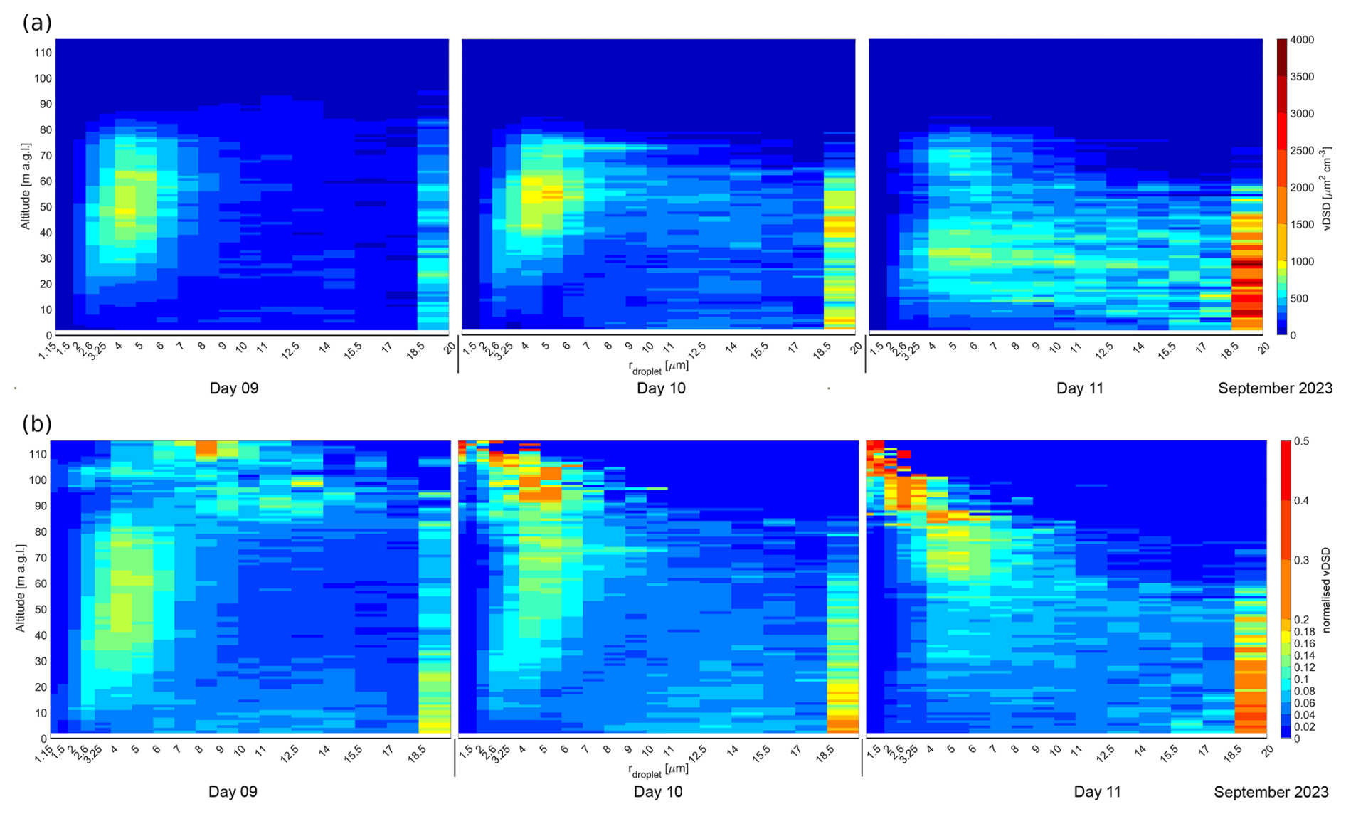
Figure 11 Vertical profile of vDSD and normalized vDSD for 9–11 September 2023 fog occurrence. Panel (a) presents the vDSD. The scale is divided into steps of 100 µm² cm⁻³ from 0 to 1000 µm² cm⁻³ and then in steps of 500 µm² cm⁻³. Panel (b) presents the normalized at each height vDSD. The figure presents what percentage of the entire spectrum at a given height is contributed by the volume of drops from a given bin.

Figure 11a indicates the altitudes where most LWC is produced and by which droplet sizes, while Fig. 11b enables analysis of the droplet spectrum in regions with low LWC – such as near the top of the fog layer or during dissipation. Apart from vDSD for the whole episode, in the Appendix (Fig. B9), vDSD is shown for each stage of fog: beginning, mature, and disappearing. This section describes how LWC, LWP, and the droplet spectrum evolve during fog occurrence for each night case.

From vDSD (Fig. 11) it is visible that most of the LWC is associated with two drop radius regions. The first region is described by an asymmetric distribution. The maximum value of the distribution is associated with a radius of 4–5 µm. The distribution has a bigger slope on the left side (droplets smaller than the maximum). The second region is a peak for droplets of radius bigger than 18.5 µm (r_>18.5). Big droplets are found in the whole range of altitudes; however, there are more of them when closer to the ground.

In the 10 m layer closest to the ground, droplets with r>18.5 µm contribute up to 40 % of the total LWC. Within this layer, the closer to the surface, the smaller the contribution to LWC from droplets with r<7 µm and the larger the contribution from droplets with r>7 µm.

Above 10 m, the situation is reversed: droplets with r< 7 µm contribute more to LWC than those with 7 µm < r< 18.5 µm. Above 40 m, with increasing altitude, the 4–5 µm peak in the normalized vDSD gradually shifts toward larger droplet sizes, reaching approximately 8–9 µm.

The maximum CTH during fog on 9 September was approximately 102 m. In most cases, the LWC above 80 m was below 0.2 g m⁻³, indicating only sparse droplets in this region. Just above the CTH, most of the water was accumulated in droplets with radii between 8 and 14 µm. With increasing height, this droplet size range decreased.

Subsequent fog nights had increasingly larger LWC at a specific height (see Fig. 6). Even though LWC reached higher values on 10 September than on 9 September, the LWP was higher on 9 September because the fog was reaching higher altitudes. The increase in LWC was related to the appearance of droplets in the size of 7–17 µm and not to the increase in the number of droplets in the size of 4–5 µm.

In the Appendix, Fig. B9 presents vDSD for three stages of fog for each day. Even in the initial stage of the fog, there were already large drops with r_>18.5, and the fog started to grow in thickness from the bottom. In the case of the fog from the nights of 9 and 10 September, with increasing height, water was stored by drops with increasingly larger radii between 2–10 µm. In the case of the fog from the night of 10 to 11 September, with increasing height, an inverse relationship occurs – increasingly smaller drops store the most water from the range of radii 2.0–18.5 µm.

In the dissipating stage of fog on 9 and 11 September, the CTH did not decrease; it remained around 80 m, while below 30 m, the vDSD shows minimal signal (bottom panels of Fig. B9), suggesting a very low droplet concentration in this region. This suggests that the fog disappeared more from the bottom than from the top.

As the profile of the dissipating fog on 10 September was taken approximately half an hour after the dissipation began, it captured only small droplets in the range of 2–7 µm at heights between 20 and 60 m. In all cases, large droplets (r_>18.5) ceased to contribute significantly to the LWC during the fog dissipation phase.

4.4 Optical, microphysical, and radiation closure

A radiative closure was performed to assess the consistency between observed radiative fluxes and the microphysical measurements. Given that the OPC-N3 is a low-cost optical particle counter, we wanted to verify whether the vertical profiles of microphysical parameters were representative of actual conditions. Since no independent method was available, we used the obtained microphysical parameters as input for radiative transfer simulations. These simulations enabled us to test whether the microphysical measurements from the OPC-N3 are consistent with the observed radiative fluxes.

Radiative transfer simulations were conducted using the Fu–Liou model in 1D mode, incorporating detailed vertical profiles of thermodynamic and microphysical properties. The model covers 6 shortwave and 12 longwave spectral bands, with input data including fog microphysics, aerosol optical properties, and surface reflectance. The fog droplet asymmetry parameter was calculated using Mie theory, based on measurements of liquid water content and droplet size. Details of the model setup are provided in Sect. 3.4.

For performing the simulations, only cases in which setup 1 (with OPC-N3) was attached to the balloon and data were properly collected were used. The simulated shortwave (SW) and longwave (LW) fluxes were compared with fluxes registered at the SolarAOT^upper and SolarAOT_lower stations. Two flights on 11 September between 05:40 and 06:22 were excluded from the radiative closure analysis due to suspected water condensation on the lower LW radiometer during fog dissipation. In total, there were 37 soundings used for analysis.

Figure 12 compares SW and LW radiation between the model and observations at the SolarAOT^upper and SolarAOT_lower stations. The scatter plots also show linear fits to the data. The left panels present the model results for clear-sky conditions based on observations from 10 September, while the right panels present results from the time when there were fog conditions during days 9–11 September.

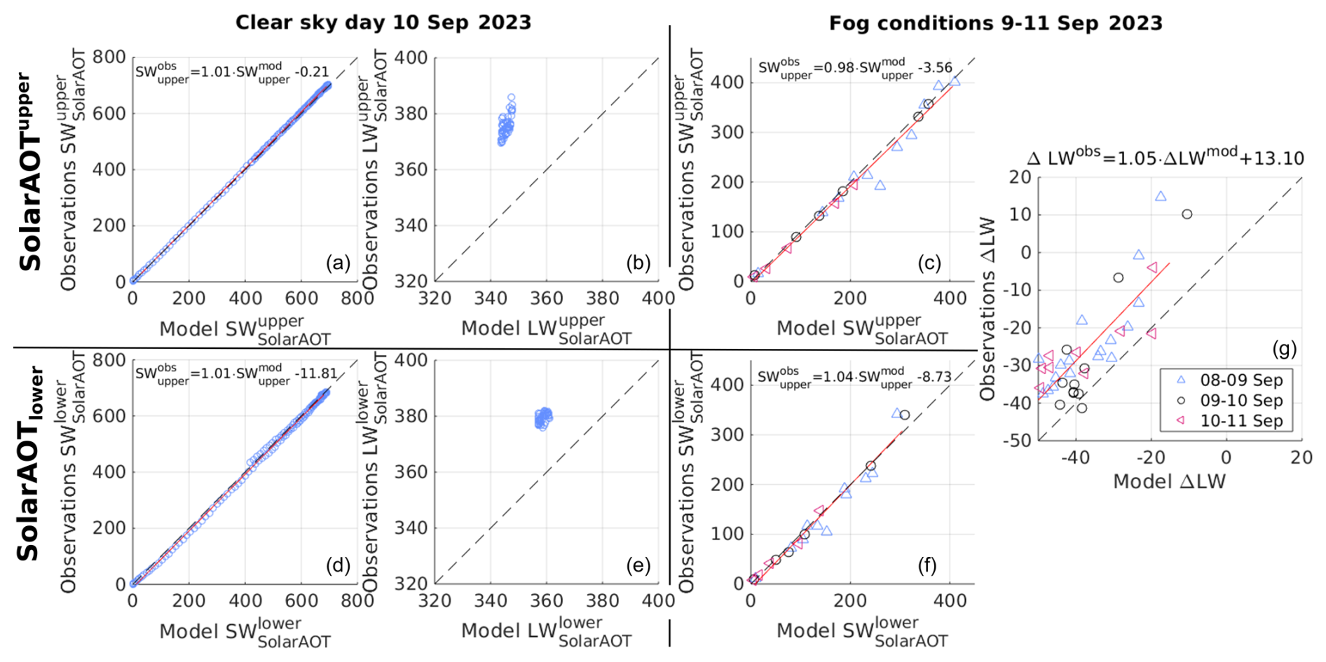
Figure 12 Scatter plots comparing observed and modeled SW (a, d, c, f) and LW (b, e, g) fluxes under clear-sky (a, b, d, e) and fog conditions (c, f, g). The last column presents the difference (Δ) between upper and lower station measurements for observed and modeled LW flux in fog conditions. The red solid line indicates the linear fit to the data. Blue triangles represent measurements from the night of 8–9 September, black circles show fog data from the night of 9–10 September, and pink triangles correspond to data collected during the night of 10–11 September 2023. The equation for each fit is shown in the corresponding panel.

Upper-air temperature and humidity profiles were taken from balloon soundings by the Polish Meteorological and Water Management Institute in Tarnów, available only twice daily (00:00 and 12:00 UTC), resulting in limited temporal resolution above 100 m. In contrast, near-surface profiles were measured more frequently on site (when fog was present). Therefore, for comparison of clear-sky conditions, only data from near the sounding at 12 ± 2 h were used.

The equation describing the relationship between the SW radiation under clear-sky and fog conditions for both stations has a relation of almost 1:1. The offset is up to −12 W m⁻².

Given the limited variation in LW downward radiation and the uncertainties introduced by sparse temperature soundings, absolute comparisons via regression provide limited insight. Instead of separate scatter plots for two stations, we present the difference in LW radiation between the upper and lower stations. The offset of the linear fit by 13.10 W m⁻² suggests that the fog implemented in the model can be too thick.

Figures 13 and 14 show the temporal comparison of SW and LW fluxes between the model and observations at the SolarAOT^upper and SolarAOT_lower stations. Black lines show the measured incoming SW and incoming LW radiation fluxes. The simulation result for clear-sky conditions is presented by the yellow dashed line, while the orange circles present the result of the simulation with implemented fog conditions, based on soundings. The difference between observations and the model is shown in Fig. 14 in the lower panel for LW flux and in Fig. 13 in the second panel from bottom for SW flux. Additionally, Table 2 presents the statistics between simulated and measured SW and LW flux for clear-sky (no fog) and fog conditions.

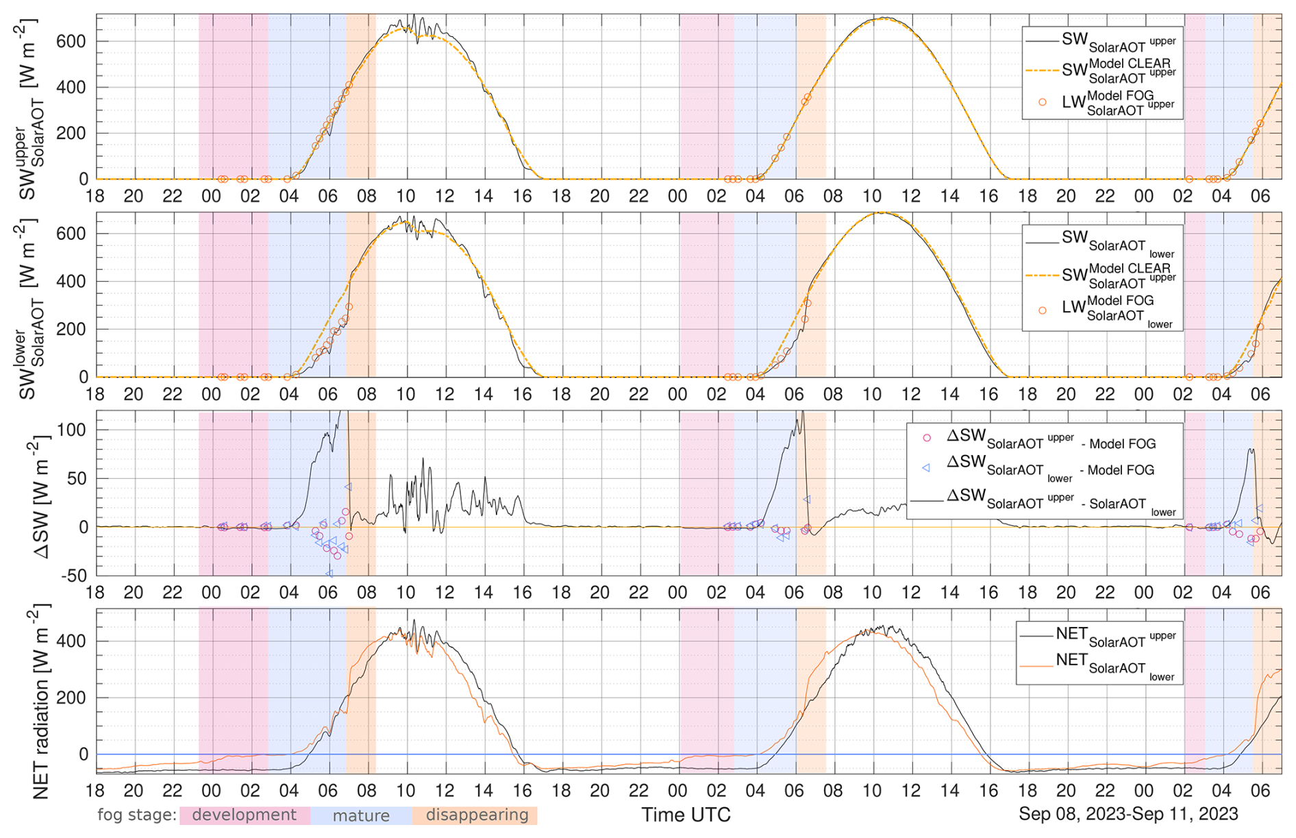
Figure 13 Incoming SW flux for SolarAOT^upper and SolarAOT_lower station. The black solid line measured data, the yellow dashed line model results for no fog conditions, and the orange circles model results for fog conditions measured by soundings. The third panel from the top presents the difference in SW flux between the upper and lower site (solid line), and pink circles represent the difference between SolarAOT^upper station and model when fog conditions were implemented. Blue triangles represent the difference between the SolarAOT_lower station and the model with implemented fog conditions. The lowest panel presents the total net radiation for SolarAOT^upper (black line) and SolarAOT_lower station (orange line).

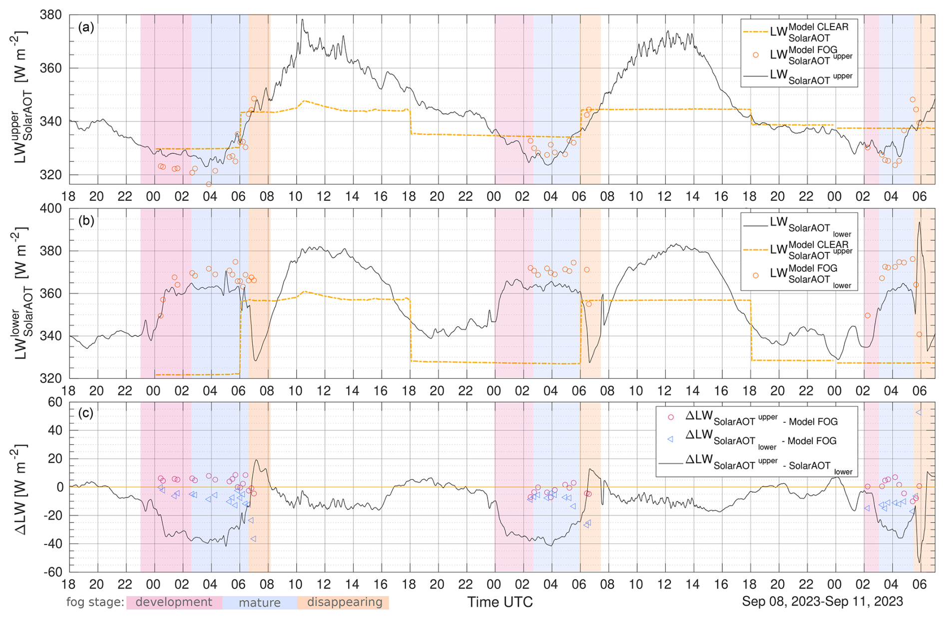
Figure 14 Incoming LW flux for SolarAOT^upper (a) and SolarAOT_lower station (b). The black solid line measured data, the yellow dashed line model result for no fog conditions, and the orange circles model results for fog conditions measured by soundings. Panel (c) presents the difference in LW flux between SolarAOT^upper and SolarAOT_lower station with the solid line, pink circles represent the difference between the upper station and the model with fog conditions implemented, and blue triangles represent the difference between lower station and model with fog conditions.

Table 2 Statistics of SW (I) and LW (IR) flux comparisons between the model and observations at both sites. The mean bias error (MBE) and root mean square error (RMSE) were calculated for each day under fog and non-fog conditions. Additionally, for 9 September, the mean MBE and RMSE for the SW radiation were computed after removing the estimated cirrus-induced bias.

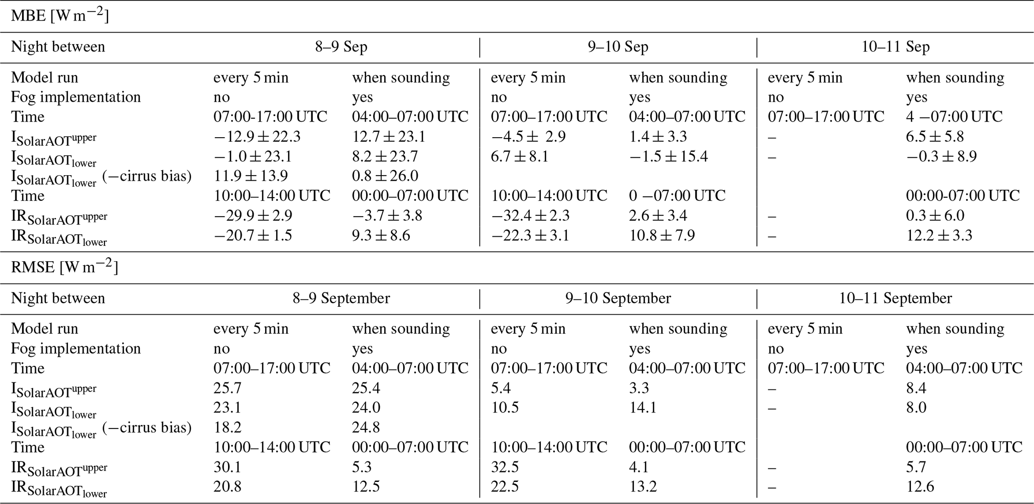
For clear-sky SW radiation, the model flux at the SolarAOT^upper station is underestimated. The root mean square error (RMSE) for 9 and 10 September is 25.7 and 5.4 m⁻², respectively. On 9 September, the SW radiation at the SolarAOT^upper station exhibits a rugged temporal pattern due to the presence of cirrus clouds. The relatively high RMSE on this day is attributed to cirrus cloud contamination, which was not accounted for in the radiative transfer model. For the SolarAOT_lower station, the RMSE is 23.1 and 10.5 W m⁻², respectively, for 9 and 10 September.

The model LW flux at both sites for clear-sky conditions is underestimated, and the RMSE exceeds 30 W m⁻² for the upper station. Running the model based solely on aerological soundings performed twice daily does not allow for an accurate representation of the diurnal variation of LW radiation. The results show significant discrepancies between the model and observations at both the upper and lower stations. To better reproduce the temporal evolution of IR radiation, more detailed information on the distribution of RH in the lower atmospheric layer is required.

The results indicate that when fog conditions are included, the model reproduces both SW and LW fluxes reasonably well at both stations. This is due to inputting more information from our soundings. For the SolarAOT^upper station, SW fluxes are slightly overestimated (by up to 12.7 W m⁻²), while LW fluxes show deviations within ±4 W m⁻².

At the SolarAOT_lower station, biases for both SW and LW fluxes remain within 12.2 W m⁻². The RMSE generally stays below 14.2 W m⁻², except under cirrus cloud conditions (9 September). The RMSE values for LW radiation at the lower station are approximately 12–13.5 W m⁻² during fog conditions, indicating that the chosen fog microphysical parameters – liquid water content LWP and r_eff – adequately represent the fog’s thermal radiative properties. The relatively low deviation suggests that the modeled fog layer produces realistic LW fluxes near the surface, supporting the suitability of the microphysical assumptions for the observed conditions. Due to model simplifications, the fog is assumed to have a constant droplet size and LWC at all heights, which may introduce some uncertainty into the results. As can be seen from the temporal comparison of LW radiation from model and data (Fig. 14), most of the model overestimation occurs during the fog decay stage; these errors may result from the lack of homogeneity or the patchwork nature of the fog during its decay. Overall, these results demonstrate that the model captures the radiative fluxes with acceptable accuracy during fog events.

4.5 Radiative fluxes during fog events

The apparatus at SolarAOT^upper and SolarAOT_lower station measures the total net radiation (NET; downward − upward SW + LW fluxes), which is presented in the lowest panel of Fig. 13. During the first night of observations, it is visible that between 00:00 and 00:44 the NET radiation at the SolarAOT_lower station changed from −24.4 to −6 W m⁻². After the development of fog, the NET radiation at the lower station was around 0 W m⁻². It became positive after sunrise. The difference between lower and upper station NET radiation during night fog was around 50 W m⁻². When the fog disappeared (07:00), there was a visible abrupt jump of 156 W m⁻² at the lower station within 15 min. For the night of 9–10 September 2023, the fog also started to develop around midnight (at 00:50 the NET radiation was −5.8 W m⁻²). NET radiation at SolarAOT_lower became positive after sunrise, and a jump of 134 W m⁻² occurred at the moment of fog disappearance at 06:20–06:40.

During the last night of observations, the NET radiation at the lower station was −44 W m⁻² at midnight, while at the upper station it was −49 W m⁻². Starting at 02:00, the net radiation gradually increased from approximately −30 m⁻² and reached 0 m⁻² at sunrise. The fog disappeared quickly, in less than 10 min; at 05:35 the NET radiation changed by 125 W m⁻².

Having information on radiation fluxes at two levels allows for investigating the sensitivity of the change in LW radiation by the fog LWP. Figure 15 shows the relationship between the modeled LWP content and the modeled difference in LW radiation between the upper and lower stations. In addition to the modeled values, the lower panel of Fig. 15 shows the relationship for the data observed at both stations and the measured LWP on the balloon in the fog. In both graphs, the data exhibit a linear relationship, with Pearson correlation coefficients and corresponding p values of −0.82 and 1.79 × 10⁻¹⁰ for the model and −0.37 and 0.02 for the observations, respectively. A straight line was fitted to the modeled data, given by the following equation:

$$\begin{array}{}\text{(17)}& \mathrm{\Delta }\mathrm{IR}=-\mathrm{1.09}\left[{\mathrm{Wg}}^{-\mathrm{1}}\right]\cdot \mathrm{LWP}-\mathrm{13.42}\left[\mathrm{W}{\mathrm{m}}^{-\mathrm{2}}\right].\end{array}$$

A straight line was fitted to the observed data:

$$\begin{array}{}\text{(18)}& \mathrm{\Delta }\mathrm{IR}=-\mathrm{0.74}\left[{\mathrm{Wg}}^{-\mathrm{1}}\right]\cdot \mathrm{LWP}+\mathrm{12.25}\left[\mathrm{W}{\mathrm{m}}^{-\mathrm{2}}\right].\end{array}$$

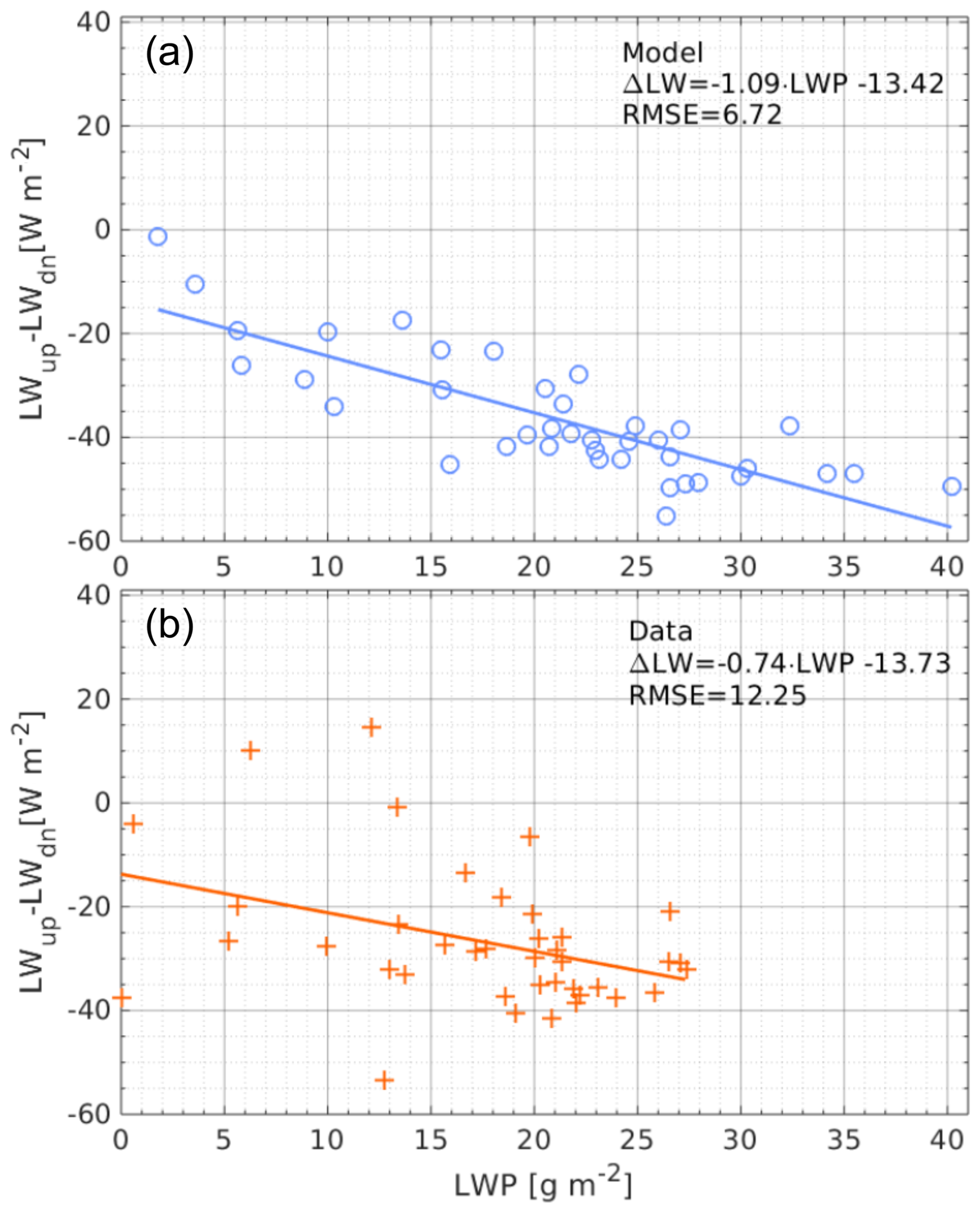
Figure 15 Relation between fog LWP (for days 9–11 September 2023) and the difference of LW downward flux between the upper and lower SolarAOT stations. The upper panel presents the radiation transfer model simulations, and the lower panel corresponds to the balloon profiles (LWP) and radiometer observations at the upper and lower SolarAOT stations.

5 Conclusions

The purpose of this study was to capture vertical profiles of the microphysical and thermodynamic characteristics within fog layers, using in situ data collected by a tethered balloon during a field campaign. This article analyzes three cases of radiative fog that occurred in the valley of the city of Strzyżów (Southeastern Poland) in September 2023. In total, 74 soundings were performed, 41 of which included measurements with the OPC-N3 sensor, enabling the calculation of droplet size spectra. The three observed cases exhibited similar meteorological conditions, including temperature (T), relative humidity (RH), and aerosol scattering coefficient at 525 nm (ASC₅₂₅). For each case, the liquid water path (LWP) exceeded 15 g m⁻², and in most instances, the fog did not transition into thick fog.

In quasi-adiabatic stratiform clouds, increases in liquid water content (LWC) are typically associated with droplet growth, with number concentrations (N_c) remaining relatively constant (Brenguier et al., 2000; Chang and Li, 2002). In contrast, our fog observations showed that LWC increases were primarily driven by increases in N_c, indicating droplet activation rather than growth via coalescence. This agrees with findings from earlier fog studies (Okita, 1962; Egli et al., 2015). The vertical structure of fog microphysics showed consistent patterns across all three cases. The effective radius (r_eff) decreases with height, as fog matured; this decrease became less pronounced. This is consistent with Okita (1962) and partially with the observations of Egli et al. (2015) (in his study, r_eff decreased with height in some cases but was mostly constant with height).

The droplet size distribution (DSD) revealed two dominant regimes: small droplets (4–5 µm) that increased in importance with height and fewer but water-rich large droplets (> 18.5 µm) of which significance decreased with height. These large droplets, though rare, contributed significantly to the total water content. Similarly in the work of Okita (1962), large droplets are mostly concentrated near the ground. Fog DSDs with small concentrations of drops greater than 30 µm were also observed in experiments conducted by Wendish et al. (1998), Gultepe et al. (2009), and Mazoyer et al. (2022). These large droplets are the result of collision–coalescence and Ostwald ripening processes. This bimodal structure is especially relevant for modeling, as current numerical weather prediction (NWP) and large eddy simulation (LES) frameworks typically use bulk microphysical schemes that assume a single-mode droplet population. These schemes are based on simplified parameters such as LWP and N_c (Bergot et al., 2007; Khain et al., 2015) and do not resolve the vertical variability or the coexistence of distinct droplet regimes. As a result, larger droplets – which play a key role in sedimentation and fog dissipation – are not properly represented, potentially leading to persistent overestimation of LWC in fog forecasts (Philip et al., 2016; Pithani et al., 2019). Incorporating full droplet spectra across the fog layer, including both small and large droplets, would allow models to more accurately simulate fog formation and dissipation (Thoma et al., 2011).

To support future fog modeling efforts, we applied the concept of equivalent adiabaticity (α_eq) across different fog stages, a relatively new parameter proposed in recent literature. The computed α_eq values ranged from 0.0 to 0.6, consistent with previous studies of fog. During one case, at the early stage of fog development, a negative value of α_eq was observed (−3.2). This negative value was attributed to an elevated LWC near the ground. In the literature, cases where LWC decreases with height in fog are rarely observed and are typically associated with thin fog layers, with CTH not exceeding 40 m (Costabloz et al., 2025; Okita, 1962; Boutle et al., 2018).

We quantified mean microphysical values for optically thin fogs in valley conditions. The fog-core LWC ranged from 0.2 to 0.4 g m⁻³, and N_c reached up to 300 cm⁻³. The mean r_eff in all cases was around 8–10 µm and decreased linearly with height. While the vertical profile of LWC could be approximated by a linear function, increasing from the ground up to approximately 60 % of the fog top height (CTH) and then decreasing toward the top, the mean N_c profile followed a parabolic shape during the nights of 8–9 and 9–10 September. In the final case (10–11 September), N_c exhibited two local maxima, located at approximately 25 % and 88 % of CTH.

In contrast to the commonly held assumption that fog dissipates primarily from the top, our observations show that in all three analyzed cases – characteristic of optically thin fog – dissipation occurred simultaneously from both the top and bottom. The dissipation process is difficult to capture, as it typically occurs within a short time frame of 15–30 min. During the dissipation stage, the region above the maximum N_c/LWC becomes compressed, likely due to solar heating from above. The maximum of N_c/LWC shifts upward to above 80 % of the fog height. We propose that the bottom dissipation is linked to surface warming caused by shortwave radiation penetrating the optically thin fog layer. As the ground heats up, the relative humidity near the surface decreases, leading to the evaporation of the smallest droplets. As no new droplets are formed, the remaining larger droplets settle and accumulate near the ground, which is reflected in increased r_eff values at the base of the fog.

Droplets with radii up to 40 µm can be described by an approximate formula for terminal velocity (u):

$$\begin{array}{}\text{(19)}& u\left(r\right)=k_{\mathrm{1}}\cdot r^{\mathrm{2}},\end{array}$$

where $k_{\mathrm{1}}\approx \mathrm{1.19}\times {\mathrm{10}}^{\mathrm{6}}$ cm⁻¹ s⁻¹ (Yau and Rogers, 1996). Using this formula, the fall velocity for droplets larger than 18.5 µm is approximately 4.07 cm s⁻¹. In the absence of droplet growth and turbulence, such droplets will be removed from a 100 m thick fog layer within about 7 min. During soundings conducted at the final stage of the fog life cycle, no large droplets were observed, indicating that they had already settled out.

Finally, we assessed the radiative impacts of fog using dual-level radiometers. At the Strzyżów location, solar and infrared radiometers are installed at two different heights (within the fog layer and above it). A linear relationship was found between infrared radiation reduction and fog water content (Pearson correlation coefficients and corresponding p values of −0.82 and $\mathrm{1.79}\times {\mathrm{10}}^{-\mathrm{10}}$ for the model and −0.37 and 0.02 for the observations, respectively). The dissipation of fog caused rapid changes (within 10–30 min) in surface radiation fluxes of up to 160 W m⁻². During fog, the mean bias between observed and modeled radiation fluxes is approximately 2 W m⁻² for shortwave (SW) and 11 W m⁻² for longwave (LW) radiation at the lower station, supporting the reliability of the retrieved microphysical inputs.

In summary, this study provides detailed observational evidence of fog microphysics and dynamics under valley conditions. These findings not only refine our understanding of fog development and dissipation but also offer actionable data for improving fog representation in weather models.

Appendix A: Temperature setup in the model

The T and RH data were taken from HYT and GY-63 and interpolated to the levels of the model. As the measurements mostly reached 115 m, above, the temperature and humidity profile was set according to the measurement from atmospheric sounding from Tarnów (WMO station 12575) done by IMGW (Polish Institute of Meteorology and Water Management). Tarnów is 60 km in a straight line from the city of Strzyżów. For a better description of the merging of data, sounding from Tarnów will be called soundingT.

To have a smooth transition between balloon sounding and the soundingT, the data from the balloon and soundingT were stitched together. For this purpose, first, the points were extrapolated so that at the stitching point, the values from both soundings were available. The procedure was performed for the last three points (highest points) from the balloon profile and the first two points of soundingT above the balloon profile. Then, for these five points, the average value weighted by the distance of the points was taken. As the soundingT does not always reach 10 km, above soundingT the standard atmosphere profile for mid-latitude summer was used.

As the profile of RH was stitched and interpolated, the precipitable water (PW) was changed. To fix this issue, the whole profile of RH was rescaled in such a way that PW is the same as the PW obtained from soundingT before interpolating.

Appendix B: Additional tables and figures

Table B1 List of abbreviations.

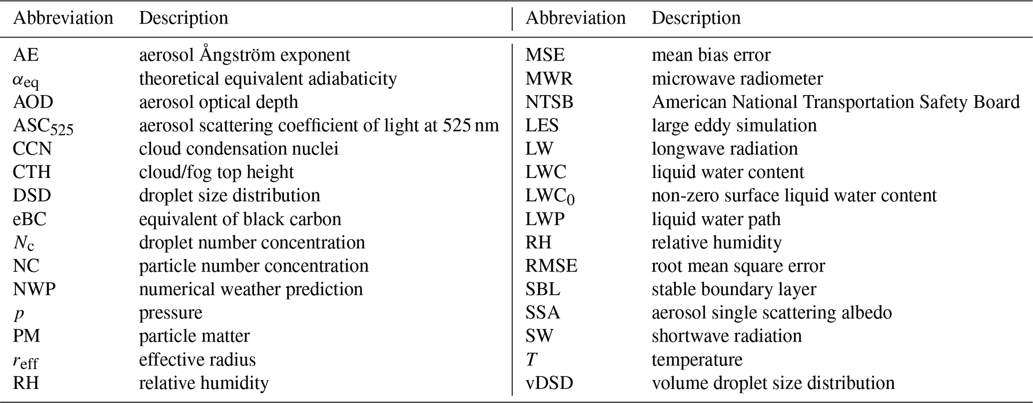
Table B2 Apparatus used during each of the soundings of case study 9–11 September 2023. Markers represent: ▸ setup with OPC-N3, • setup with radiosonde, ▴ setup with OPC-N3 and radiosonde, and □ problems with collected data (soundings with partially recorded data were not taken into further analysis.

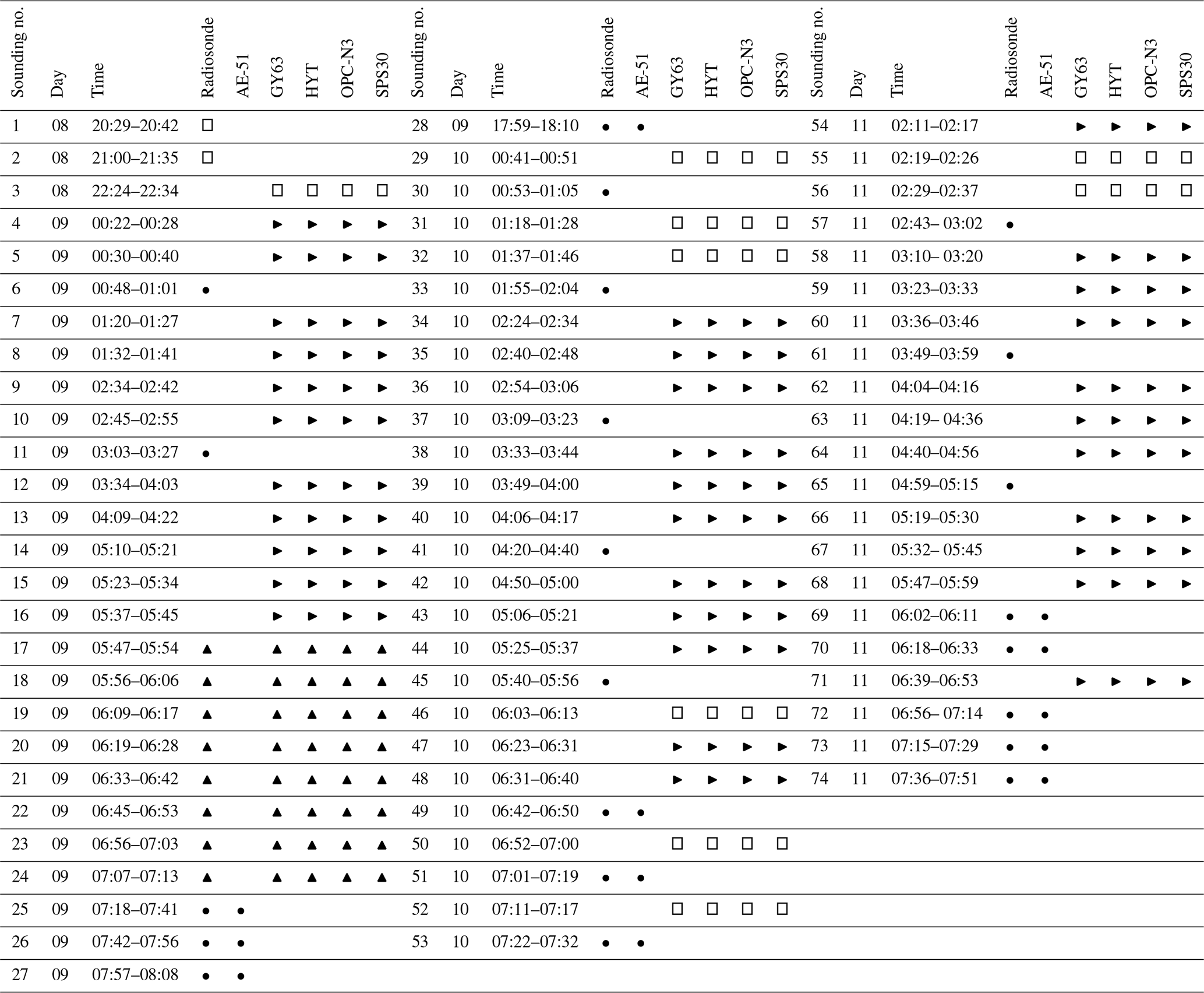
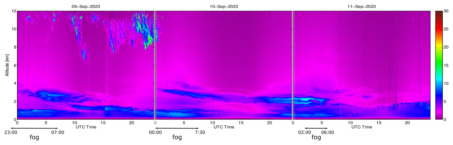
Figure B1 Temporal variability of 510 M lidar-range-corrected signal (at 532 nm) from the level of the upper station up to 12 km between 9 and 11 September 2023.

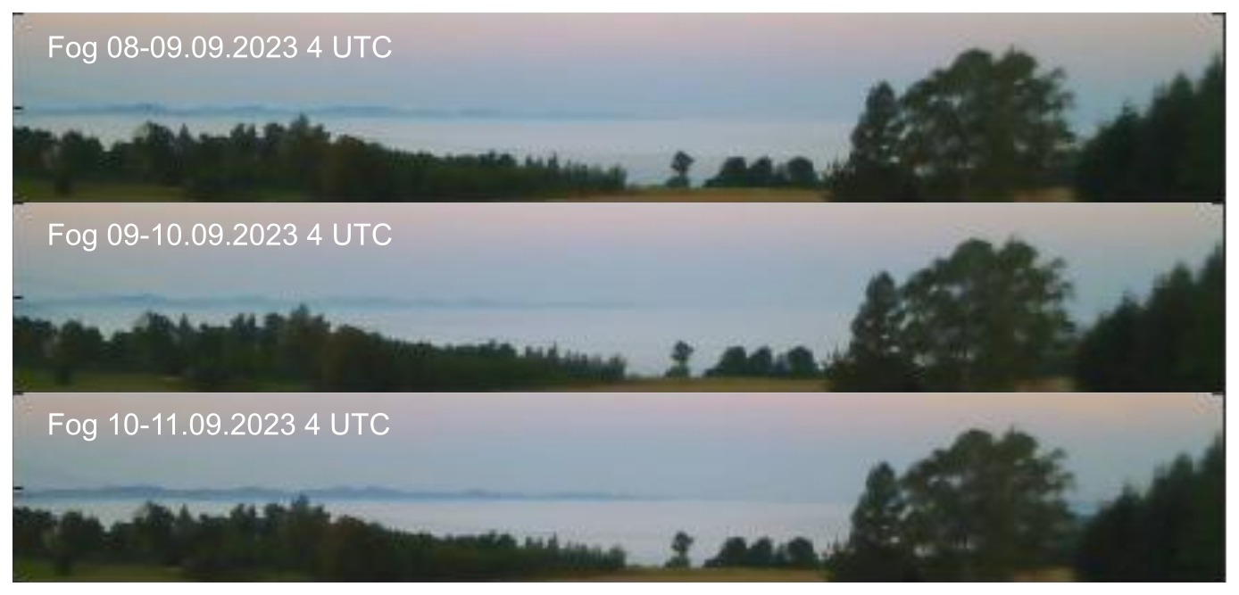
Figure B2 Visualization of radiation fog top. Photos were taken with the camera at the SolarAOT^upper station at 04:00 UTC each day.

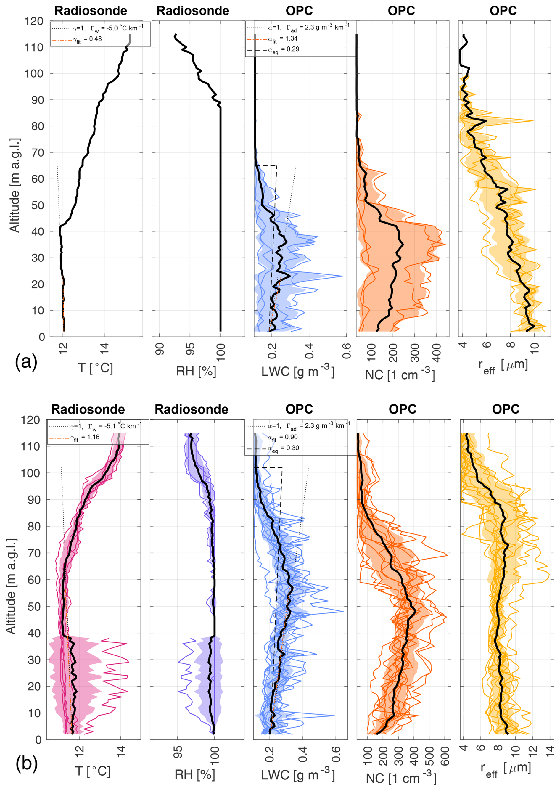
Figure B3 Panels present specific quantities measured by the balloon for each stage of fog observed during the night of 8–9 September 2023. (a) Development stage of fog. (b) Mature state of fog. Detailed description in the caption of Fig. B4.

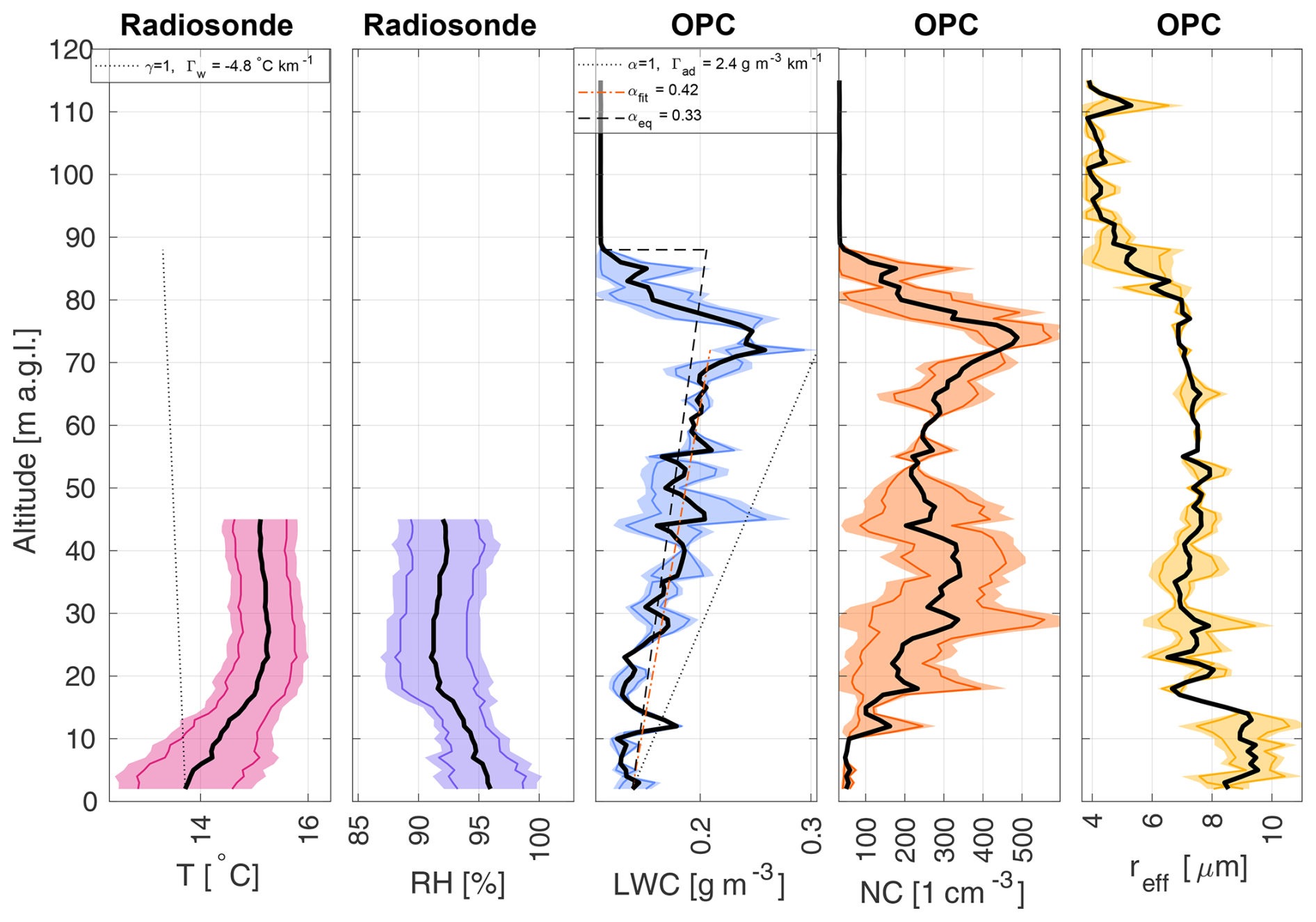
Figure B4 Disappearing stage of fog. Panels present specific quantities measured by the balloon for each stage of fog observed during the night of 8–9 September 2023. From left: T from Vaisala radiosonde RS41, RH from Vaisala radiosonde RS41, N_c, and r_eff within the fog. Each colored line represents one balloon profile. The black thick line represents the mean of all the soundings, and the colored area represents the range between ± standard deviation from the mean. In the T plot, the dotted line presents the lapse rate, and the dashed red line presents the linear fit to T from 2 m to the height of maximum mean LWC. In the LWC plot, the dotted line presents the LWC adiabatic lapse rate, and the dashed red line presents the linear fit to LWC from 2 m to the height of maximum mean LWC.

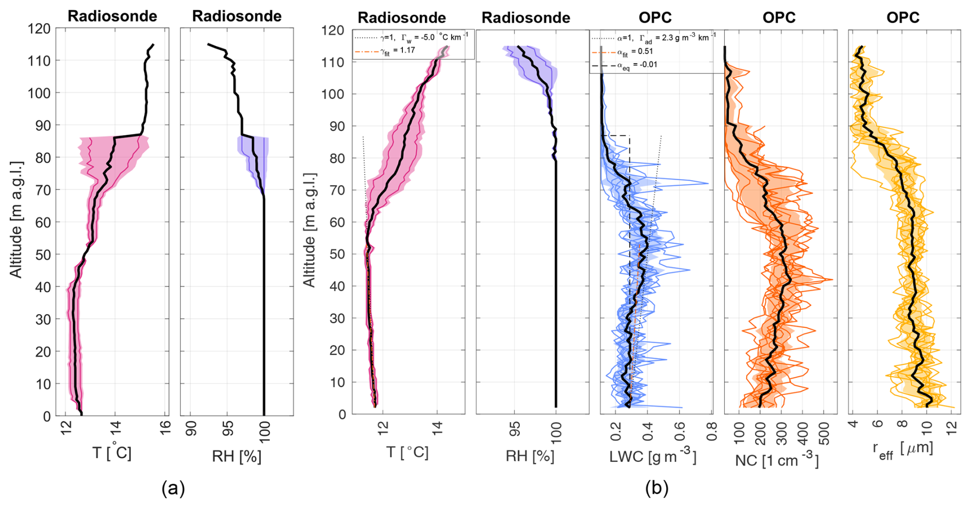
Figure B5 Panels present specific quantities measured by the balloon for each stage of fog observed during the night of 10–11 September 2023. (a) Development stage of fog. (b) Mature state of fog. Detailed description in the caption of Fig. B6.

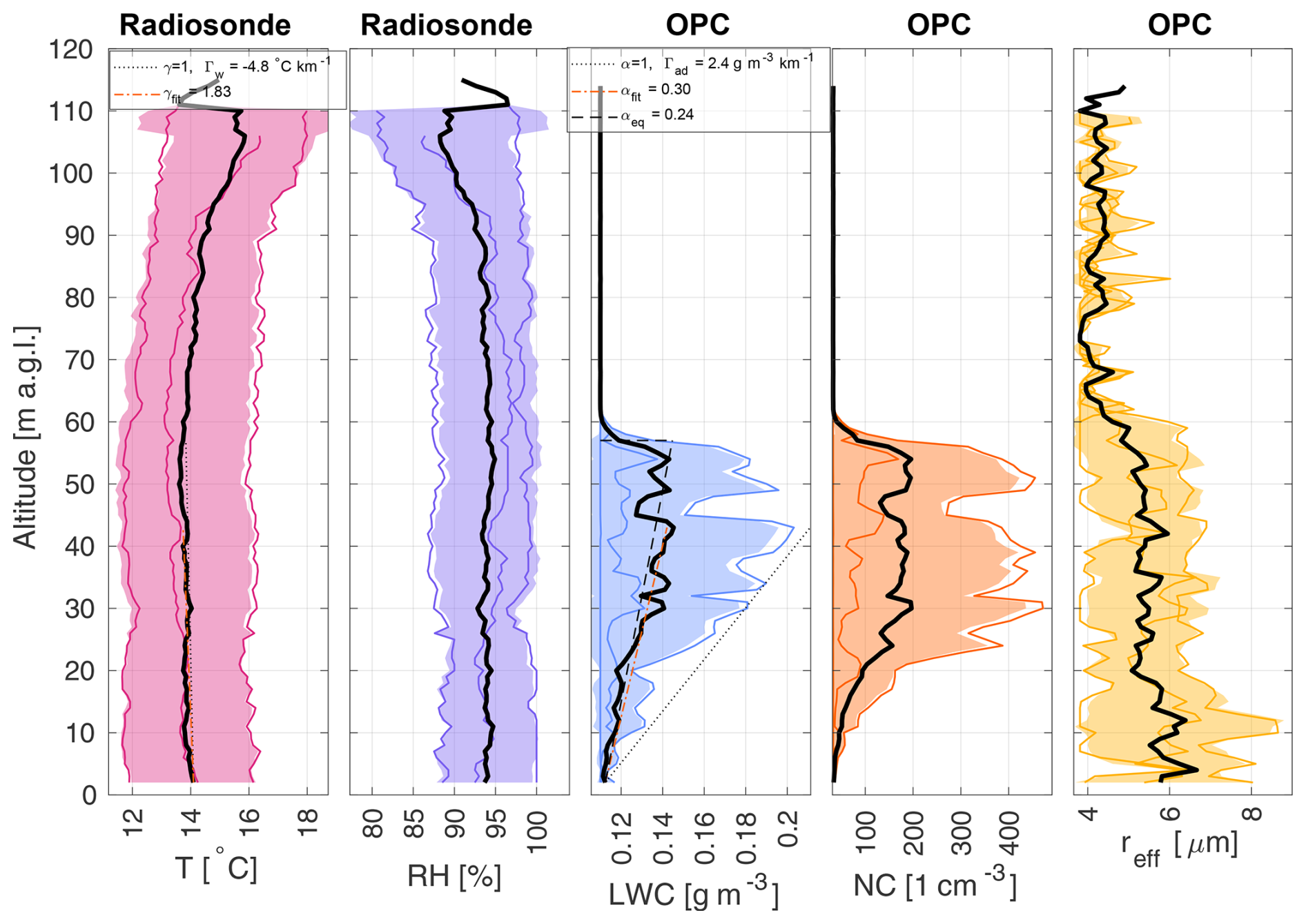
Figure B6 Disappearing stage of fog. Panels present specific quantities measured by the balloon for each stage of fog observed during night of 9–10 September 2023. From left: T from Vaisala radiosonde RS41, RH from Vaisala radiosonde RS41, N_c, and r_eff within the fog. Each colored line represents one balloon profile. The black thick line represents the mean of all the soundings, and the colored area represents the range between ± standard deviation from the mean. In the T plot, the dotted line presents the lapse rate, and the dashed red line presents the linear fit to T from 2 m to the height of maximum mean LWC. In the LWC plot, the dotted line presents the LWC adiabatic lapse rate, and the dashed red line presents the linear fit to LWC from 2 m to the height of maximum mean LWC.

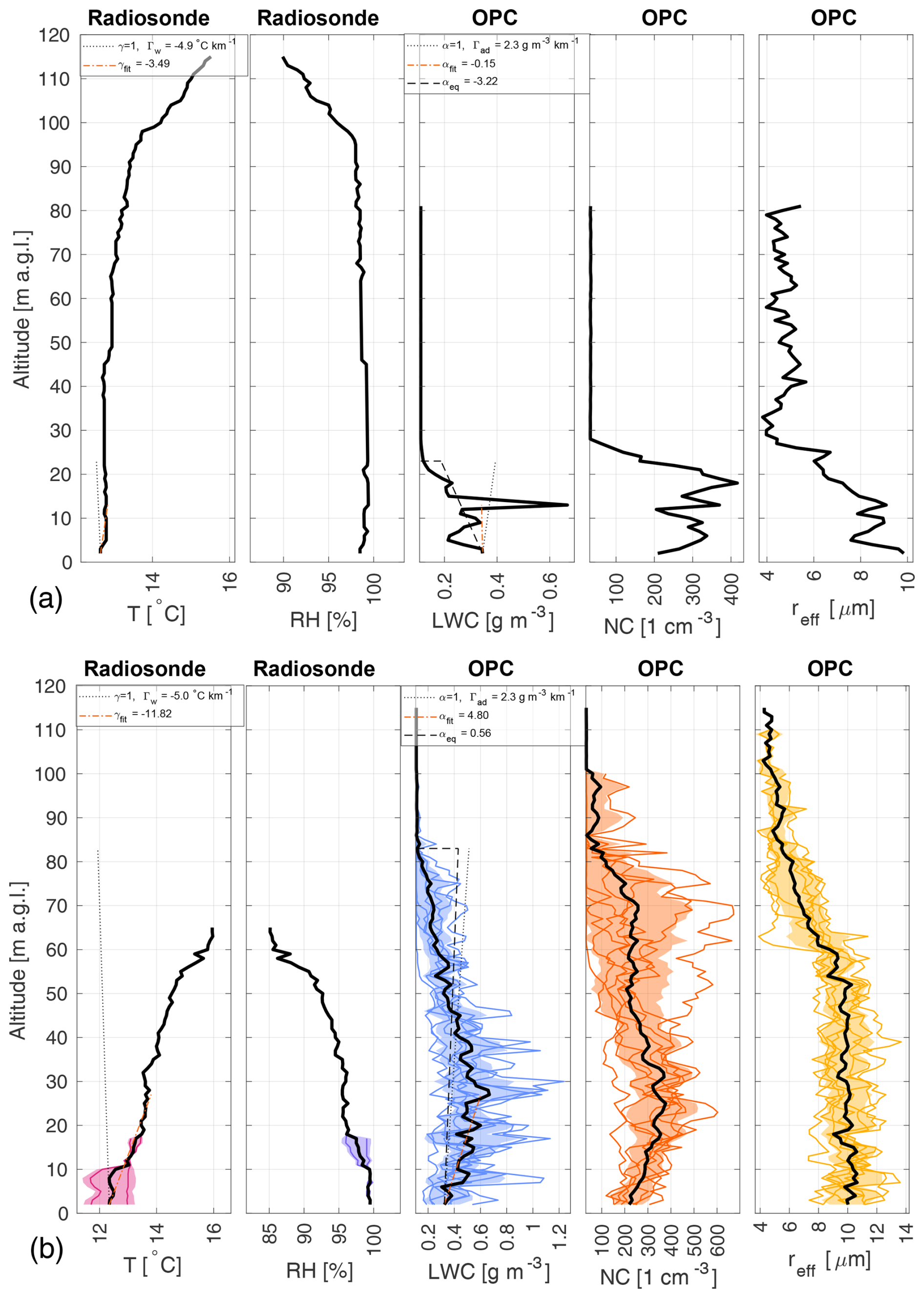
Figure B7 Panels present specific quantities measured by the balloon for each stage of fog observed during the night of 10–11 September 2023. (a) Development stage of fog. (b) Mature state of fog. Detailed description in the caption of Fig. B8.

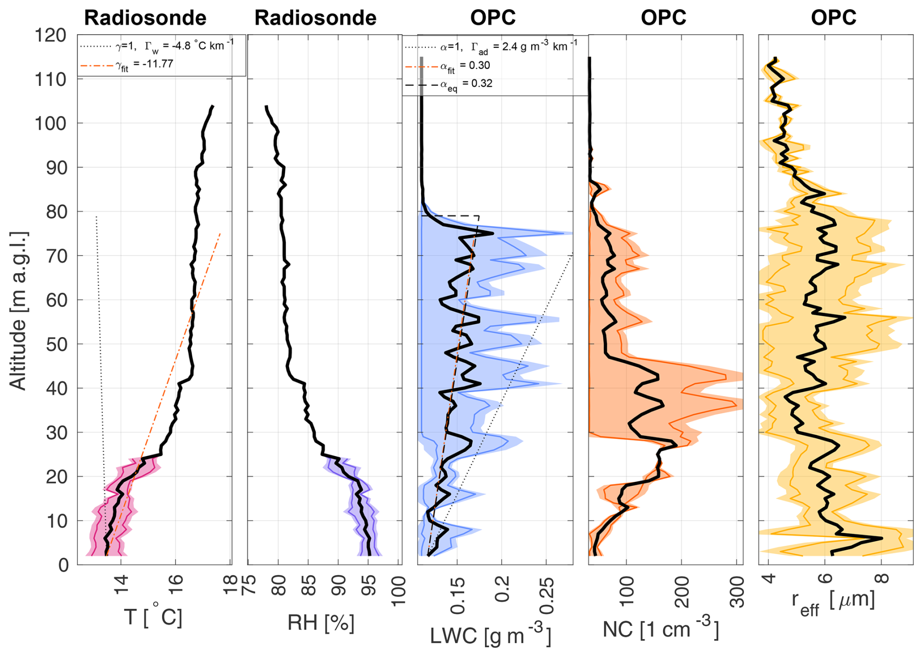
Figure B8 Disappearing stage of fog. Panels present specific quantities measured by the balloon for each stage of fog observed during the night of 10–11 September 2023. From left: T from Vaisala radiosonde RS41, RH from Vaisala radiosonde RS41, N_c, and r_eff within the fog. Each colored line represents one balloon profile. The black thick line represents the mean of all the soundings, and the colored area represents the range between ± standard deviation from the mean. In the T plot, the dotted line presents the lapse rate, and the dashed red line presents the linear fit to T from 2 m to the height of maximum mean LWC. In the LWC plot, the dotted line presents the LWC adiabatic lapse rate, and the dashed red line presents the linear fit to LWC from 2 m to the height of maximum mean LWC.

.

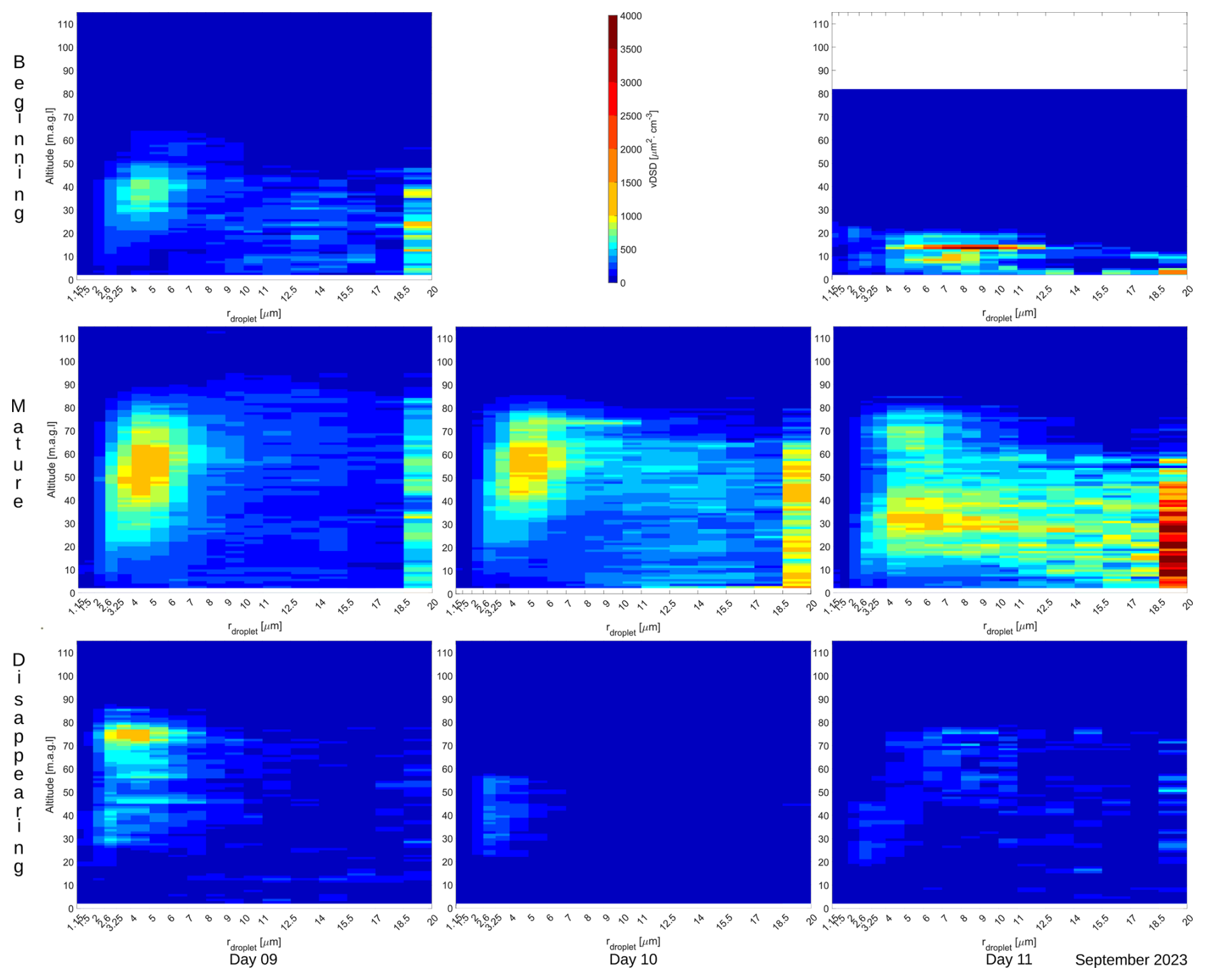
Figure B9 Profiles with height of vDSD for 9–11 September 2023 fog occurrence. Different days are in columns, in rows from the top: beginning, mature, and disappearing stage of fog.