Application of PRIM for understanding patterns in carbon dioxide model-observation differences

Reducing uncertainties in regional carbon balances requires a better understanding of CO₂ transport in synoptic weather systems. Here, we apply the Patient Rule Induction Method (PRIM), a data-mining method to identify high-density regions for a target-class within an input parameter space, to airborne observations of potential temperature, wind speed, water vapor mixing ratio, and CO₂ dry mol fraction gathered during the Atmospheric Carbon and Transport (ACT)-America Summer 2016 and Winter 2017 campaigns. ACT observations were targeted at expert-designated cases of fair weather and near-frontal warm and cold sector air at atmospheric boundary-layer, lower-, and higher free tropospheric levels (ABL, LFT, and HFT, respectively).

We investigate atmospheric characteristics of these pre-defined cases and associated CO₂ model-observation-differences in the mesoscale WRF-Chem model. PRIM results separate winter- and summertime observations as well as observations from ABL, LFT, and HFT with enrichment factors of 4.0–20.5 inside the PRIM box compared to the entire dataset but cannot distinguish between near-frontal warm and cold sector observations in the higher free troposphere. Analyzing of the parameter space constrained by PRIM, we find that large magnitude model observation differences preferentially associated with times when atmospheric conditions are less typical. This association suggests that PRIM could provide a useful tool for isolating atmospheric conditions with large-magnitude and non-Gaussian CO₂-residuals for targeted transport model evaluation and to potentially improve inversion results during synoptically active periods.

1 Introduction

The terrestrial biosphere continues to be the largest source of uncertainty in the global carbon budget and exhibits large inter-annual and regional variation (Friedlingstein et al., 2023). While the global atmospheric carbon dioxide budget is well constrained (Ciais et al., 2013), regional contributions from the terrestrial biosphere are less well understood (Peiro et al., 2022; Crowell et al., 2019; Peylin et al., 2013). Because biospheric models disagree substantially in magnitude (Huntzinger et al., 2013) and drivers (Huntzinger et al., 2017) of terrestrial carbon uptake, quantifying regional contributions to the carbon cycle remains difficult.

Atmospheric inversion, which provides a top-down alternative, for estimating terrestrial carbon fluxes, typically seeks to minimize the difference between a set of observed and modeled atmospheric CO₂ mole fractions ([CO₂]) by adjusting a set of a priori carbon fluxes (Tarantola and Valette, 1982; Tarantola, 2005; Bousquet et al., 1996). These inversions are thus sensitive to both prior flux model and atmospheric transport model errors. Disentangling their relative contributions to overall inversion error remains a challenge.

Because transport error constitutes a major source of uncertainty in atmospheric inversion (e.g. Baker et al., 2006; Stephens et al., 2007; Chevallier et al., 2010; Díaz-Isaac et al., 2014; Lauvaux and Davis, 2014; Feng et al., 2019a), and because atmospheric CO₂ is transported through mid-latitude weather systems on global (Parazoo et al., 2008, 2011, 2021; Barnes et al., 2016; Schuh et al., 2019) and continental scales (Hurwitz et al., 2004; Pal et al., 2020; Hu et al., 2021), improving the representation of mid-latitude synoptic systems in transport models could potentially reduce inversion uncertainties (Davis et al., 2021). Impacts of mid-latitude weather systems on atmospheric [CO₂] are multifaceted and complex. For example, advection in synoptic systems concentrates upstream CO₂ patterns (Keppel-Aleks et al., 2011, 2012) and is a dominant driver for day-to-day CO₂ variability within the atmospheric boundary layer (Parazoo et al., 2008, 2011). Also, CO₂ fluxes respond strongly to synoptic scale gradients (Parazoo et al., 2012) trough modification of drivers for ecosystem-atmosphere CO₂ exchange (Chan et al., 2004). Transport model resolution is important for accurate modeling of synoptic conditions and corresponding CO₂ transport and spatio-temporal variability within weather systems (Agustí-Panareda et al., 2019).

Despite their importance, synoptically active conditions are sparsely sampled, because cloud interference limits satellite remote sensing of column CO₂ (e.g. Parazoo et al., 2008; Wang et al., 2023) and airborne networks, e.g. the NOAA Carbon Cycle and Greenhouse Gases (CCGG) Aircraft Program (Sweeney et al., 2015), tend to avoid storm systems for operational reasons.

At the same time, transport models capable of resolving the atmospheric boundary layer as well as the dynamic features of synoptic weather systems including fronts are also highly sensitive to the effects of atmospheric boundary layer (ABL) parameterizations affecting ABL-depth and vertical mixing (Díaz-Isaac et al., 2014, 2018), and consequently inversion results (Lauvaux and Davis, 2014). The application of such models therefore requires targeted and careful transport model validation using atmospheric observations designed to capture CO₂ and atmospheric features sampled within and around mid-latitude weather systems.

The NASA funded Atmospheric Carbon and Transport (ACT)-America Earth Venture Suborbital Mission (Davis et al., 2021) was conducted to provide observations of CO₂ and CH₄ mole fractions within the central and eastern U.S. – a dominant region of North American terrestrial carbon fluxes – for evaluating and improving regional flux inversion systems. ACT-America flight planning aimed to address the gap in observations of mid-latitude weather systems through targeted sampling of pre-, post, and cross-frontal flights applying expert-designated cases corresponding to the ABL, lower, and higher free troposphere (LFT and HFT, respectively) as well as synoptic sector (near-frontal warm, near-frontal cold, and fair weather air) (Davis et al., 2021) hypothesizing that weather systems show distinct effects on CO₂-dynamics at each altitude and airmass.

ACT-America data was, for example, used to diagnose missing processes in the Carnegie-Stanford-Approach (CASA) model, a commonly used flux prior in regional inversion (Feng et al., 2021a) and to infer systematic underestimation of flux-seasonality in the inversion models examined during the Orbiting Carbon Observatory-2 (OCO-2) version 9 Model Intercomparison Project (Cui et al., 2021, 2022). The data also show underestimation of cross-frontal [CO₂] differences (Pal et al., 2020; Zhang et al., 2022) in models with implications modeled CO₂ weather and atmospheric inversion. Similarly, while atmospheric transport models were overall capable of reproducing observed [CO₂] in the central and eastern U.S., model biases were strongly related to season and synoptic conditions such that warm sector airmasses near frontal boundaries were associated with larger magnitude model-observation differences compared to fair weather air (Gerken et al., 2021).

Given the importance of atmospheric transport models for constraining regional and global CO₂ fluxes through inversion, we need a better understanding of atmospheric conditions associated with synoptic weather systems and their impacts on atmospheric carbon transport. We use the Patient Rule Induction Method (PRIM; Friedman and Fisher, 1999) to (1) determine whether expert designations are a useful tool for analyzing processes related to atmospheric carbon transport related to synoptic activity, (2) including the extent to which atmospheric characteristics (temperature, wind speed, moisture, and [CO₂]) are characteristic of synoptic conditions and altitude as well as (3) whether magnitudes of [CO₂] model-observation differences can be linked to synoptic weather conditions. This investigation aims to further characterize the variability of [CO₂] model-observation differences and to aid in the development of future atmospheric inversion systems that might include more fine-tuned assumptions about prescribed transport model and prior flux errors.

2 Data and Methods

This work applies PRIM (Friedman and Fisher, 1999) to ACT-America data (Wei et al., 2021) from the Summer 2016 and Winter 2017 flight campaigns.

2.1 ACT-America Aircraft Observations

We use airborne data from the the ACT-America: L3 Merged In Situ Atmospheric Trace Gases and Flask Data, Eastern USA data set (Data Citation:  Davis et al., 2018, updated 4 March 2019), available at Oak Ridge National Lab Distributed Active Archive Center (ORNL-DAAC) and described in Wei et al. (2021).

In addition to CO₂ dry mole fractions (Picarro G2401-m cavity ring down spectrometer), we use potential temperature (θ) and water vapor mixing ratio (MR) as well as u- and v-component winds obtained from the aircrafts' Meteorological Instrument Suite and Embedded Global Positioning System/Inertial Navigation System. ACT-America flights were planned to sample fair weather conditions and synoptic systems through cross-frontal of synoptic systems as well as pre- and post-frontal flights sampling near-frontal warm and cold airmasses. ACT observations were manually tagged with airmass information according to aircraft location and equivalent potential temperature, wind, and trace gas changes across fronts. Additional details about instruments, data products, and airmass identification can be found in Wei et al. (2021) and dataset documentation (Davis et al., 2018).

Similar to Gerken et al. (2021), we exclusively use data from level-leg flight segments, i.e. without substantial altitude changes, from the Summer 2016 and Winter 2017 flight campaigns conducted from 18 June to 28 August 2016 and 30 January to 10 March 2017. During both flight campaigns, ACT-America study domains of Mid-Atlantic, Mid-West, and South-Central U.S. were sampled using Wallops/ Norfolk (Virginia), Lincoln (Nebraska), and Shreveport (Louisiana) as flight bases. See Table S1 in the Supplement and Gerken et al. (2021) for additional details about flight dates and flight locations. Level-leg data are separated into three expert-designated categories defined by altitudes above ground level:

1. atmospheric boundary layer (ABL; < 1.5 km),

2. lower free troposphere (LFT; 1.5–4.0 km), and

3. higher free troposphere (HFT; ≥ 4 km).

ACT flight planning, with flights commencing in mid-morning, ensured that ABL observations were indeed located within the ABL irrespective of actual ABL height. LFT and HFT levels were designed for separating the region of the troposphere that is frequently affected by convective mixing and clouds from higher regions more likely to represent atmospheric background conditions (Baier et al., 2020; Sweeney et al., 2015). We further designate airmasses as near-frontal warm sector, near-frontal cold sector, as well as fair weather in this study. While fair weather air could be further separated into warm and cold airmasses, we decided against doing so to focus on the role of mid-latitude weather systems in atmospheric carbon dioxide dynamics.

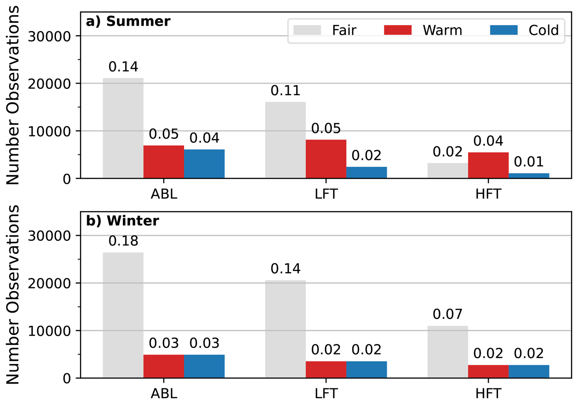
Figure 1 Share of ACT-America Observations during (a) Summer 2016 and (b) Winter 2017 flight campaigns separated into expert-designated classes based on altitude-level and airmass. The bar labels show the relative fraction of observations in each class.

Table 1 Distribution of ACT-America campaign observations counts by season, level [atmospheric boundary layer (ABL), lower (LFT), higher free troposphere (HFT)], and airmass (Fair weather, near-frontal Warm, near-frontal Cold).

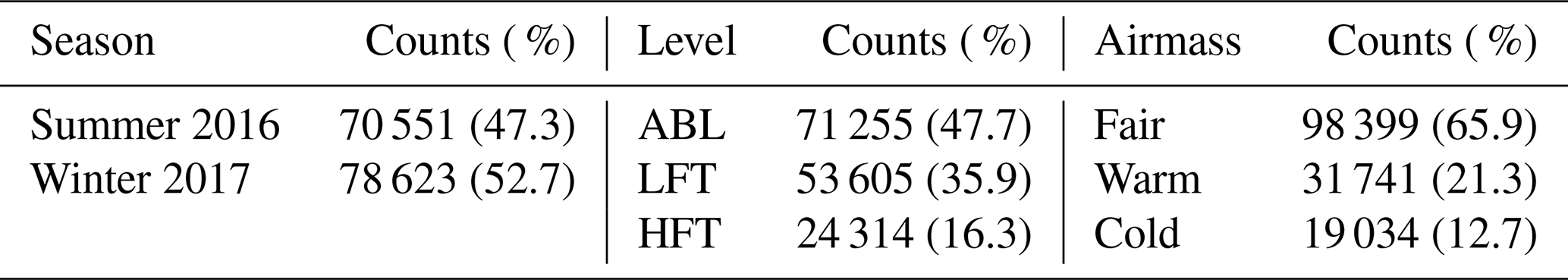
All data are averaged to 5 s temporal resolution, which corresponds to an approximate spatial resolution of 500–600 m based on the airspeed of the aircraft. Data without airmass information, with unusually high [CO₂], indicative of CO₂ point sources, ([CO₂] > 430 ppm), and unrealistic wind velocities (u or v > 100 ms⁻¹) are discarded before the analysis. The [CO₂] level of 430 ppm was chosen to be substantially higher than values typically found in the dataset such that few data points were eliminated. However, there were several instances when the planes flew in vicinity to industrial or fossil fuel power plants with [CO₂] greatly exceeding 430 ppm. The remaining 149 174 observations used in this study have an approximately even distribution between summer and winter, but the sampling varies considerably with respect to level and airmass. Specifically ABL and fair weather air make up 48 % and 66 % of observations, respectively (Table 1). Separating the data by season, level, and airmass (Fig. 1) reveals a stark imbalance in the number of fair weather and near-frontal warm and cold airmass observations for all levels and seasons except for HFT during summer, when few fair weather observations exist. There are also mores warm sector observations than cold sector observations at all levels during summer, while this is not the case during winter.

2.2 CO₂ Model-Observation-Differences

To address whether atmospheric conditions associated with expert-designated cases have an impact on potential inversion model performance, we use [CO₂] model observation differences (also referred to as residuals) calculated by subtracting observed [CO₂] from modeled [CO₂] along the aircraft flight path using a nearest neighbor approach in space and time. Modeled [CO₂] were obtained using the mesoscale WRF-Chem v3.6.1 (Fast et al., 2006; Grell et al., 2005; Powers et al., 2017) covering North-America at 27 km horizontal resolution and with 50 levels between surface and 50 hPa (20 levels are within the lowermost 1 km). Choices for model parameters and the detailed setup including CO₂ surface fluxes from CarbonTracker and lateral boundary conditions are documented as the baseline experiment in Feng et al. (2019a, b) and further discussed along with [CO₂] residuals in Gerken et al. (2021). Model output for all ACT-America campaigns is archived in the Pennsylvania State University Data-Commons (Data Citation:  Feng et al., 2020) and ORNL-DAAC (Data Citation:  Feng et al., 2021b).

2.3 PRIM

The PRIM-method (Friedman and Fisher, 1999), originally referred to as bump-hunting by the developers, is a data mining technique, seeking to identify regions of interest within a multi-dimensional parameter space. Simple rules about input variables are used to find a combination of variable ranges that define a region, in which a designated variable of interest occurs at a higher than usual frequency. PRIM has also been applied to a wide range of environmental and political scenario analysis and decision support including scenario discovery for biofuel transition (Bryant and Lempert, 2010) and pollution control (Hadka et al., 2015).

The PRIM method proceeds by successively peeling away rectangular slices of the input parameter-space to yield a series of boxes or regions with an increasingly higher mean value of the target (Bryant and Lempert, 2010). This process is referred to as a peeling trajectory.

To a reader unfamiliar with PRIM, this process is best described through a toy example with a single dimension: Consider the case of applying PRIM to temperature observations throughout the year and using “Summer” as the expert-designated case of interest (i.e. the target). In each step of the peeling-trajectory, PRIM would successively constrain the temperature range that defines the so-called PRIM box to exclude temperature observations with comparatively few occurrences that belong to the “Summer” target-case until the box no-longer contains any “non-Summer” observations. Therefore the density of the “Summer” target-case is maximized within the PRIM box while the box size is becoming increasingly smaller. During this process, an increasing number of observations that belong to the “Summer” target-case would be excluded as a trade-off such that the box, would provide increasingly less coverage of summertime observations contained in the dataset. Adding additional variables such as moisture, would result in a higher dimensionality of PRIM boxes, while the process itself would remain the same.

In summary, each step in the PRIM peeling trajectory is defined by (Bryant and Lempert, 2010):

PRIM box.

The subset of the input parameter space that is preferentially associated with the target case. The extent of the PRIM box therefore characterizes environmental conditions most likely associated with a pre-defined target- (or expert-designated) case.

box density.

The ratio of the target cases to the total number of cases inside the PRIM box, which is analogous to the precision metric in a classification problem.

box coverage.

The share of total observations of the target case that are contained in the PRIM box. This is analogous to recall or sensitivity metrics in a classification problem.

It is important to emphasize that following along the peeling trajectory presents a trade-off between increasing the density of target observations within the PRIM box and excluding an increasing number of target observations as the box-size is reduced, thus concentrating target observations inside the box. Given a predefined target (or in this study expert-designated) case, PRIM thus characterizes the target based on its preferential location within the input parameter space. Therefore, PRIM can be used to identify and describe the typical environmental conditions associated with a target case of interest.

In contrast to conventional and strict clustering methods, this approach explicitly accounts for overlaps between target cases though the density-coverage trade-off and PRIM rules are designed to be simple and interpretable.

PRIM is further described in the Supplement and Fig. S1 in the Supplement shows an example of how PRIM boxes are constructed in a multidimensional space and their relation to density and coverage levels and associated input variable ranges.

We apply the Hadka (2022) PRIM (release: v0.5.0) implementation to ACT-America aircraft data. We define each unique combination of season (Summer 2016, Winter 2017), level (ABL, LFT, HFT), and airmass (Fair weather, near-frontal Warm, near-frontal Cold) from Table 1 for a total of 18 expert-designated cases to identify lower and upper bounds for potential temperature, water vapor mixing ratio, u- and v-wind velocities, as well as [CO₂] typically associated with each pre-defined case (collectively referred to as PRIM box). PRIM output for each case is saved and a coverage level of 0.75, which reflects the trade-off between coverage and density inherent to PRIM and includes the majority of target observation for each case while excluding extreme environmental conditions, is selected for analysis.

3 Results

3.1 Atmospheric Conditions during ACT

To provide context for interpreting PRIM results,an overview of observed atmospheric conditions during the ACT Summer 2016 and Winter 2017 campaigns is shown in Fig. 2. In line with expectations, [CO₂] is generally lower in summer due to biospheric uptake, while θ and MR are higher in summer than winter. Median u-wind velocities are larger during the winter campaign and generally indicate westerly winds. For v-winds, fair weather and warm sectors tend to be associated with southerly flow in ABL and LFT, while cold sectors tend to exhibit northerly flow. For HFT, there is no clear relationship between airmass and meridonal wind. [CO₂] and MR variability is larger during summer compared to winter, while θ, u- and v-wind exhibit more variability in winter than summer. There is notably a much larger variation of MR in the free troposphere (LFT & HFT) during summer compared to winter that is potentially attributable not only to temperature, but also to convective massflux.

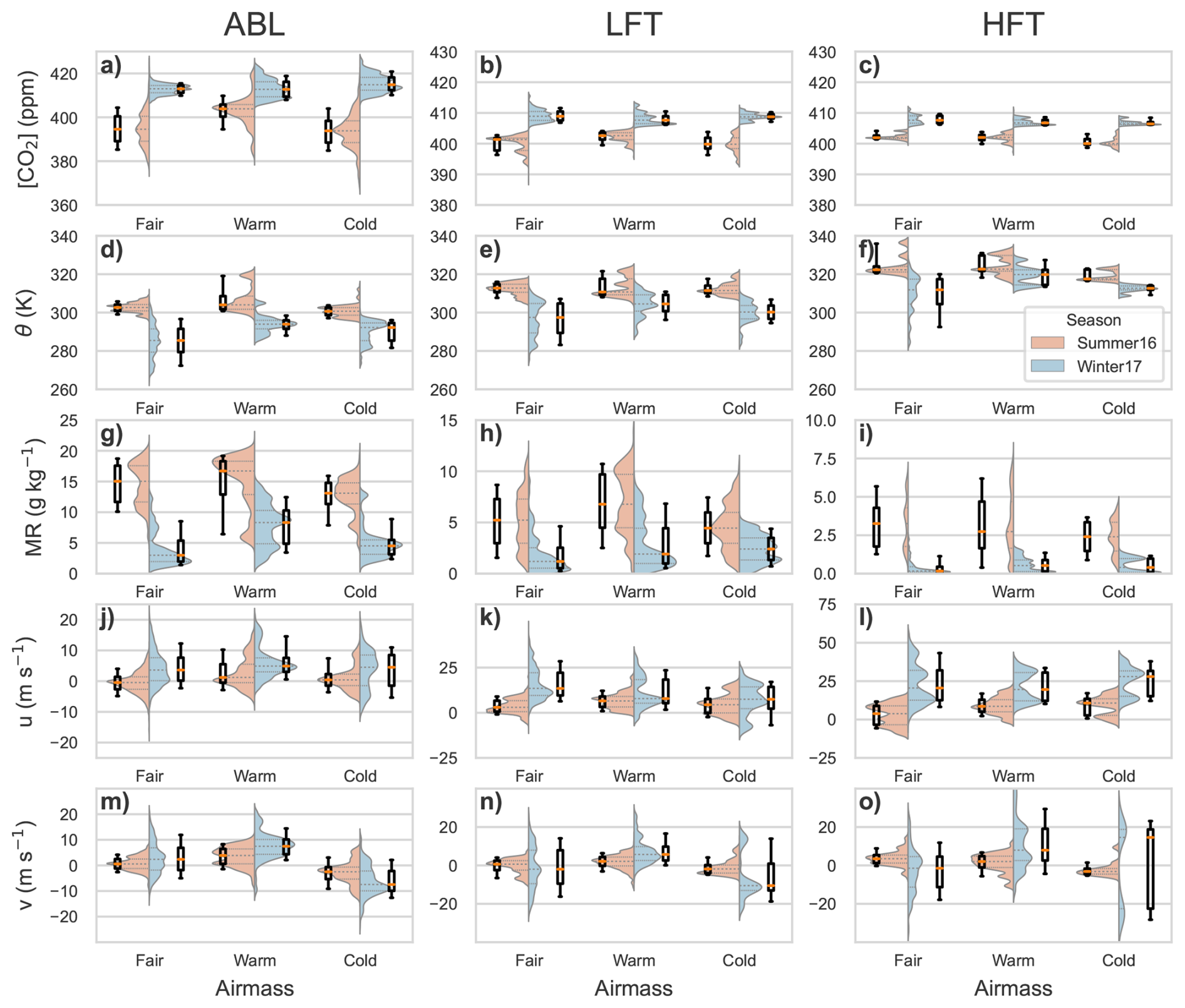
Figure 2 Kernel density plots of observed atmospheric conditions during ACT Summer 2016 (red) and Winter 2017 (blue) campaigns for (a–c) [CO₂], (d–f) potential temperature (θ), (g–i) water vapor mixing ratio (MR), (j–l) zonal wind speed (u), and (m–o) meridional wind speed (v). Data are separated into vertical levels corresponding to atmospheric boundary layer (left column), lower free troposphere (center column) and higher free troposphere (right column) and airmass. Overlaid box-whisker plots show median (orange line), interquartile range (box), as well as 10th and 90th percentiles (whiskers). Interquartile range and median are also shown on the kernel density plots as solid and dashed lines.

3.2 PRIM Results

We first establish the applicability of PRIM to the ACT-America dataset and investigate how environmental conditions constrained by PRIM align with pre-designated categories.

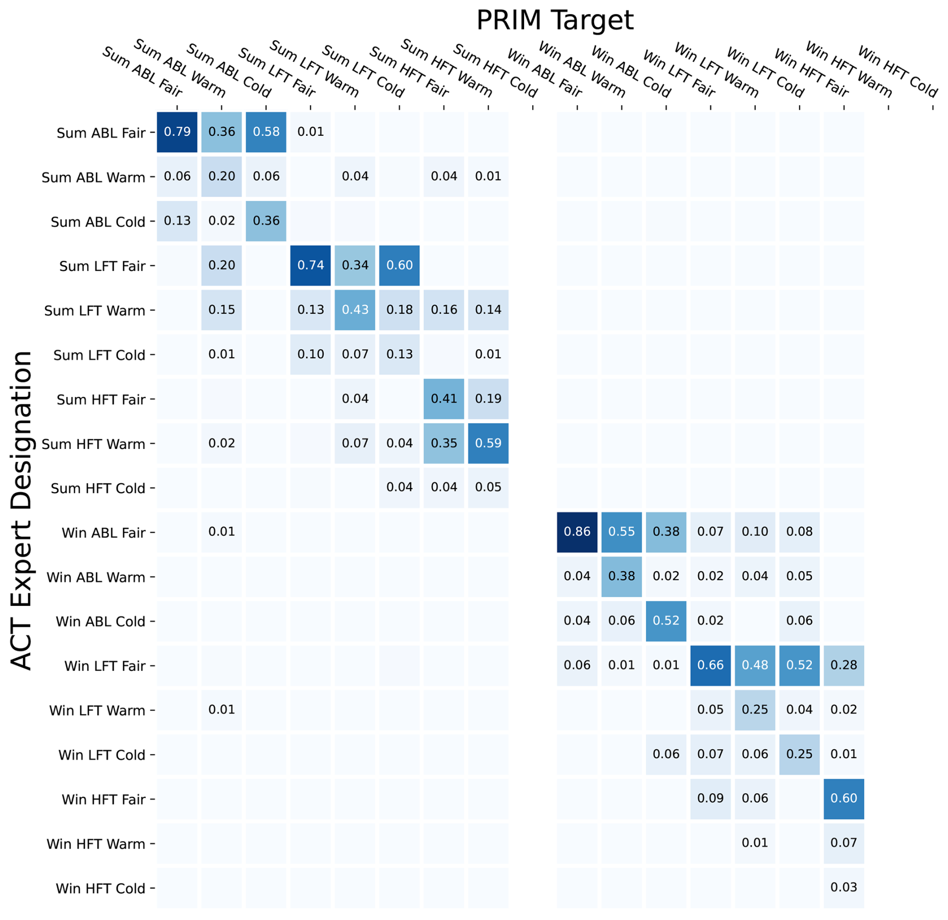
Figure 3 Comparison of PRIM target-designation and actual pre-designated ACT-Classification by experts within the parameter space identified by the PRIM box. Values on the diagonal show the fraction of target observations (i.e. the density) for each class within the parameter space designated by PRIM at the chosen coverage of 0.75, while the remainder of each column shows the occurrence of observations from other ACT designations within the PRIM box. Values in each column will add to 1.0 and labels for classes with a share of less than 0.01 of observations are omitted for clarity.

Table 2 PRIM enrichment, defined as the share of observations belonging to the expert-designated target class inside the PRIM box (box density) compared to the total share of observations in the ACT-dataset, for each class at 75 % coverage. Values >1 indicate enrichment compared to the overall dataset and that PRIM successfully identified a high-density region of the target class within the environmental parameter space.

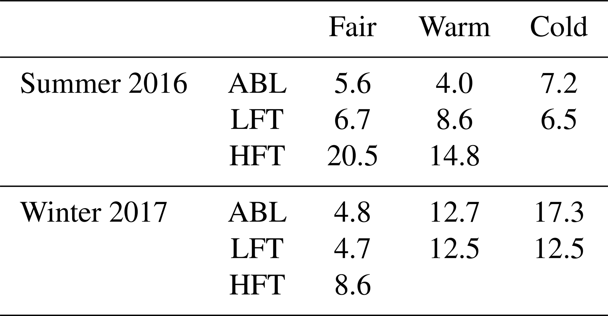
Results (Table 2 and Fig. 3) show that PRIM is capable of identifying winter- and summertime observations as well as observations from ABL, LFT, and HFT levels based on atmospheric conditions. PRIM does not successfully identify within the dataset near-frontal cold sector air in the HFT for both seasons and warm sector HFT air during winter. When successful, PRIM box densities are 4–20 times higher than the respective shares of the entire ACT-dataset (Fig. 1b), showing that PRIM is capable of identifying regions in the environmental parameter space that can be interpreted as typically associated with the expert-designated target classes.

We hypothesize that PRIM's failure to separate out warm and cold sectors in HFT is likely due to the small number of HFT near-frontal warm and cold sectors observations in the ACT dataset. Additionally, results are consistent with HFT air being more akin to the continental background (Baier et al., 2020; Sweeney et al., 2015) and less affected by synoptic perturbation such that differences in near-frontal warm and cold airmasses are smaller compared to lower levels.

Near-frontal warm and cold sector observations are less well separated by PRIM from fair weather air masses, but warm sector air is rarely found within PRIM designations of cold sector air (and vice-versa). For example, box densities for ABL warm and cold sectors are 0.20 and 0.36 for summer and 0.38 and 0.58, respectively during winter, while box densities for fair weather conditions are much higher at 0.79 and 0.86, respectively. Higher box densities for fair weather conditions can be explained by the fact that there is a larger number of fair weather flight days (14 out of 25 and 15 out of 24 d for Summer 2016 and Winter 2017, respectively) with more elaborate sampling patterns (Davis et al., 2021) and thus more observations in the ACT data-set and because there is a substantial overlap in atmospheric conditions between fair weather conditions and near-frontal warm and cold sector air (see Fig. 2, left column). During summer, 36 % of observations within the PRIM box designating ABL warm sector conditions belong to instances with expert-designation of fair weather ABL and another 36 % belong to observations attributed to LFT air (20 % LFT fair and 15 % LFT warm). During winter, 55 % of observations within the PRIM box for ABL warm sector conditions belong to the expert-designation of ABL fair, while only 1 % are pre-classified as free tropospheric.

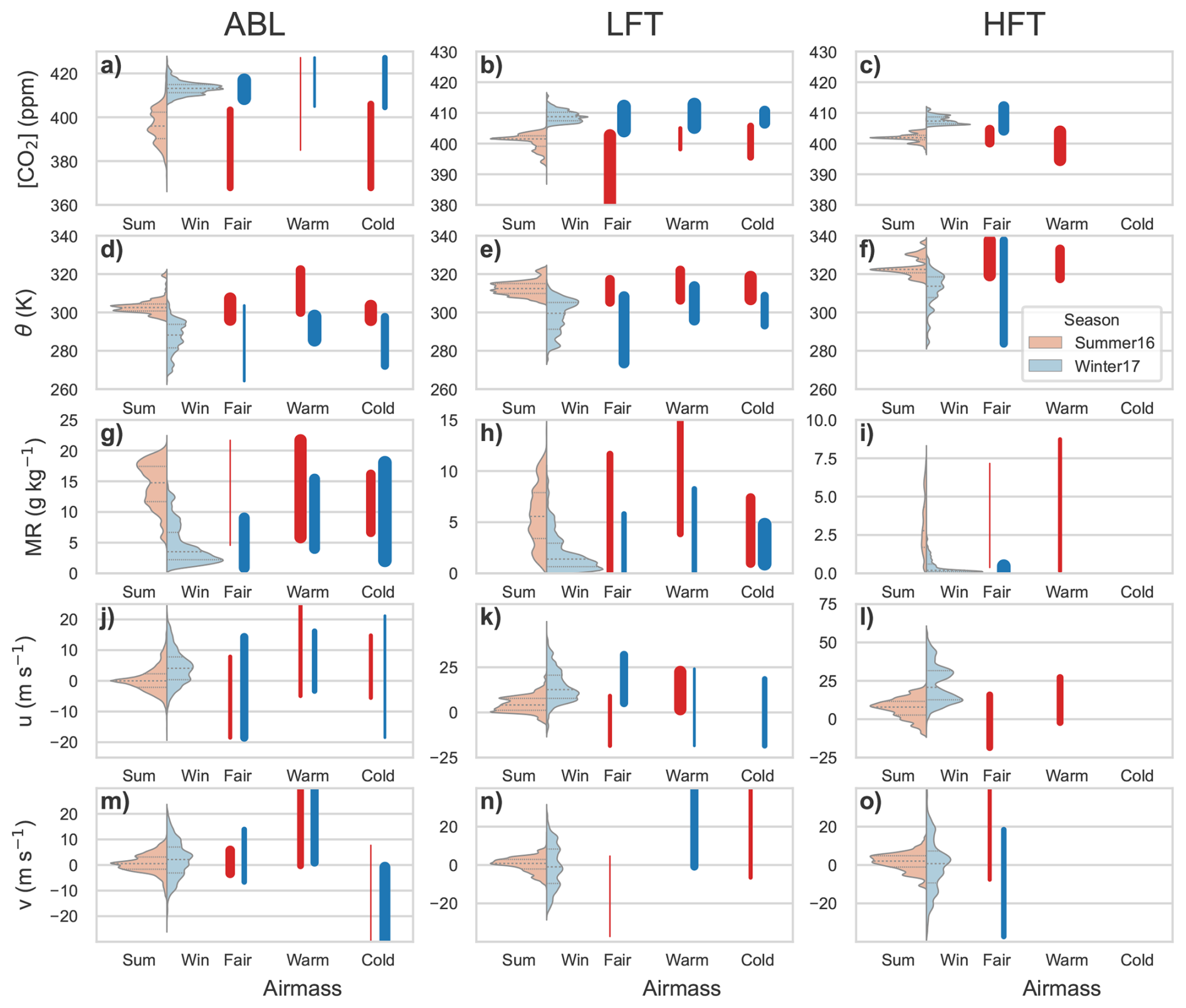
Figure 4 Summary of PRIM box parameters during ACT Summer 2016 (red) and Winter 2017 (blue) campaigns at a coverage level of 0.75 for (a–c) [CO₂], (d–f) potential temperature (θ), (g–i) water vapor mixing ratio (MR), (j–l) zonal wind speed (u), and (m–o) meridional wind speed (v). Data are separated into vertical levels corresponding to atmospheric boundary layer (left column), lower free troposphere (center column) and higher free troposphere (right column) and airmass. Vertical bars show the range of typical atmospheric variables of ACT observations in each class. The thickness of the bar indicates the importance of each variable for defining PRIM boxes and the absence of a line shows that PRIM did not use that variable to constrain the box. Violin plots show the kernel density estimate of ACT observations for all airmass types. Please note that the y-scale between subplots varies to account for differences in range between ABL, LFT, and HFT levels.

The main advantage of the PRIM method compared to many other data-mining techniques is that results are explainable through the found box parameters (Fig. 4 and Table S2). At the chosen coverage level of 0.75, the parameters of the box can be interpreted as the typical value range for each atmospheric variable for every expert-designated case defined by combinations of season, level, and synoptic condition (e.g. Summer + ABL + fair weather). PRIM also provides a ranking of importance for each of the variables used in the classification depending on the order which atmospheric variables are used to constrain the overall parameter space.

We generally find potential temperature and moisture to be most important for characterizing boundary-layer air, while [CO₂] is found to be less important except for fair weather in winter. However, [CO₂] together with potential temperature and moisture are important when classifying air from LFT. HFT air during winter is characterized by low MR and high [CO₂], while summertime HFT air exhibits high θ and comparatively low [CO₂], as expected.

Interestingly, the limited separation of warm sector ABL air during summer from LFT air, can be explained by the fact that PRIM considers high MR and high θ as the most important variables (Fig. 4d, g), and ACT observations find similarly high MR within the LFT warm sector consistent with vertical convective moisture transport and maritime inflow from for example the Gulf of Mexico (Fig. 2h).

PRIM also identifies meridional wind as a factor in identifying ABL warm and cold sectors, as warm airmasses are associated with southerly flow, while cold airmasses exhibit northerly flow. PRIM's identification of the weak association between summertime ABL air with low [CO₂] in cold sectors and high [CO₂] in warm sectors is consistent with depletion of CO₂ in northerly air due to the continental summertime carbon sink, while southerly airmasses coming from the Gulf of Mexico and the Atlantic represent a higher CO₂ background.

The lack of separation between air designated as LFT cold sector during winter and designated fair weather LFT air (Fig. 3) is due to PRIM's box designation based on MR, [CO₂], and θ (Fig. 4b, e, h) yielding a parameter space that is largely encompassed by the parameter space designating the PRIM box for fair weather LFT air making cold sector air not separable from fair weather air due to the substantial overlap in atmospheric conditions.

3.3 CO₂ Residuals and Atmospheric Conditions

Given the necessity to accurately characterize transport and prior flux errors for atmospheric CO₂ inversion, it is useful to examine the behavior of [CO₂] model-observation-differences associated with the expert-designated cases and to examine whether [CO₂] residuals are randomly distributed across atmospheric conditions.

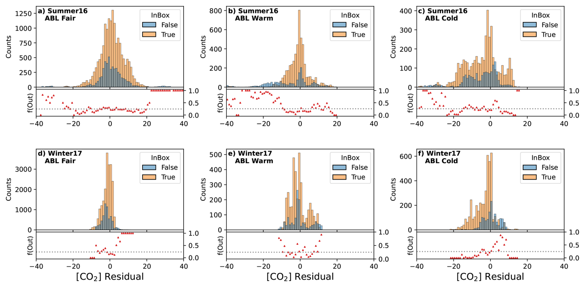
Figure 5 Histogram of [CO₂] model observation differences for ABL air separated by Summer (upper row) and Winter (lower row) and airmass. Red bars indicate the number of observations inside the PRIM box (at 75 % coverage) indicative of the typical parameter space of atmospheric conditions associated with that expert-designated case, whereas blue bars are for atmospheric conditions outside the PRIM box and thus for atmospheric conditions less likely to be encountered. The lower panels show the fraction of occurrences that are outside of the PRIM box. The dashed line indicates the average out of box fraction (1-coverage).

For each expert-designated case, PRIM was used to constrain the atmospheric parameter space spanned by potential temperature, water vapor mixing ratio, u- and v-wind velocities, and [CO₂], such that it covers 75 % of target observations. Vice-versa 25 % of target observations belonging to lower density regions of the parameter space are excluded. Therefore, the PRIM box can be interpreted as the typical atmospheric conditions associated with each expert-designated case, while observations outside the PRIM box are associated with less frequently encountered atmospheric conditions for the expert designated case.

If [CO₂] model-observation-differences were independent of atmospheric conditions, large magnitude and small magnitude [CO₂] residuals would randomly distributed within the entire parameter space, and we would encounter no difference in the occurance of large and small magnitude residuals within parameter space constrained for each case (i.e. the PRIM box). However, based on the histogram of residuals (Fig. 5) this is not the case. Instead, we find that the largest magnitude [CO₂] residuals are over-represented for atmospheric conditions outside the PRIM box for each expert-designated case. This behavior is stronger during summer (Fig. 5a–c), when [CO₂] residuals show a much wider distribution with heavy tails or large magnitude residuals, as opposed to winter, when CO₂ residuals are more constrained. Notably, both [CO₂] residuals and whether they are associated with typical or less frequently encountered atmospheric conditions are more symmetric for fair weather air in summer, while large magnitude negative residuals (i.e model underestimates CO₂ compared to observations) dominate in near-frontal warm and cold sector airmasses of synoptic systems. For winter, Fig. 5d–f) we find a similar association of large magnitude [CO₂] residuals with less common atmospheric conditions for fair weather and near frontal warm sector airmasses, but not for the cold sector, where less frequently encountered atmospheric conditions are found for moderately positive [CO₂] residuals. The differing behavior of cold-sector winter can be explained by the fact, high CO₂ levels are used to designate the PRIM box for the cold sector. Therefore, periods during which the model underestimates CO₂ are more frequently found inside the box.

We proceed to define the the center 50 % of [CO₂] residuals as small residuals and residuals beyond the 5th and 95th percentiles as large residuals. Comparing the share of small (Fig. 6) confirms the previously observed association of large magnitude [CO₂] residuals with conditions outside of typical atmospheric parameter range delineated by the PRIM box.

In other words, the [CO₂] model-observation-mismatch is large, when atmospheric conditions deviate from the typical range for each case. This finding holds true in our analysis for all considered airmasses in winter and warm sector air during summer, while substantial differences exist between fair weather and cold airmasses during summer.

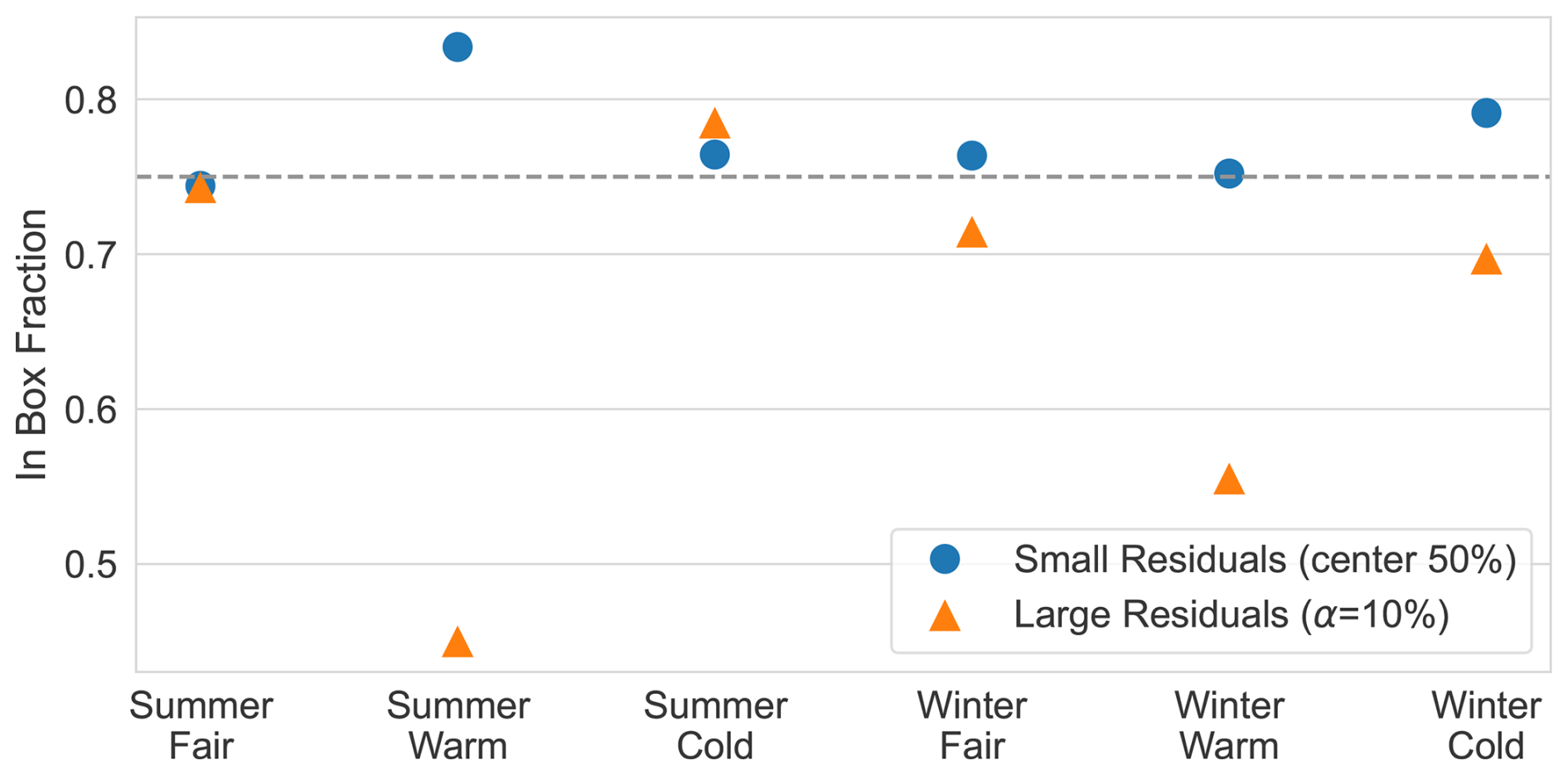
Figure 6 Fraction of ABL data found within the PRIM (75 % coverage, dashed line) box for small (25–75th percentiles) and large magnitude (<5th and >95th) [CO₂] residuals separated by season and airmass. Data below the dashed line indicate that residuals are less likely associated with typical environmental conditions for that expert-designated case.

4 Discussion

We proceed to discuss the PRIM's characterization of airmasses, model-observation-mismatches, and study limitations.

4.1 PRIM Characterization of Airmasses

Because synoptic weather systems are a major contributor to horizontal and vertical CO₂ transport in mid-latitudes on continental and regional scales (Davis et al., 2021), we investigated whether PRIM was able to characterize atmospheric conditions associated with expert-designations of synoptic conditions and altitude. While it is customary for classification methods to perform a train-test split of the data or to validate the model with not-yet seen before data to ensure that the model has predictive skill, the focus of our analysis is to extract information about the target cases from the pre-existing ACT-America dataset, which more akin to clustering where a ground truth is not known than classification. Importantly, we do not claim that PRIM has predictive skill, but that PRIM is able to identify high-density regions associated with expert-designated cases within the ACT-America dataset.

Our results (Fig. 4) show that atmospheric conditions for the analyzed cases are identifiable by PRIM and can thus be considered distinct, which includes the separation of lower tropospheric and higher tropospheric air. Our results showing similarities between warm sector ABL air and LFT air are consistent with vertical mixing due to frontal uplift of boundary-layer air and convective instabilities carrying carbon flux information from terrestrial ecosystems (Parazoo et al., 2008, 2011). Our results thus highlight the potential utility of ACT data for evaluating CO₂ vertical mixing strength, which is a major factor for inversion accuracy (Peylin et al., 2013; Schuh et al., 2019; Stephens et al., 2007).

While PRIM had difficulties in separating out near-frontal cold and warm sector airmasses highlight fair weather air, which which could also be classified into warm and cold airmasses depending on its airmass history, PRIM achieved good separation for near frontal warm and cold sector air. In line with expectations, meteorological variables and particularly moisture and potential temperature were of higher importance for PRIM classification than [CO₂] despite persistent and large cross-frontal [CO₂] gradients (Pal et al., 2020; Zhang et al., 2022; Wang et al., 2023) that highlight the importance of horizontal CO₂ transport associated with fronts.

PRIM's use of water vapor mixing ratio and southerly winds to distinguish warm sector air from the cold sector is consistent with marine air from the Gulf of Mexico and the Atlantic. Lagrangian modeling of airmass origin for ACT-flights (Gaudet et al., 2021) confirmed the preferential oceanic origin of warm sector air, whereas cold sector stem from the north with extended residence time over North American forests and agricultural region.

PRIM's inability to distinguish near frontal warm and cold sector air from fair weather conditions in the higher free troposphere is in line with the hypothesis that synoptic systems have limited impacts on upper tropospheric air. HFT air would thus represent background conditions (Parazoo et al., 2021; Baier et al., 2020) with respect to CO₂ while terrestrial carbon fluxes and vertical transport associated with synoptic systems act on vertically homogeneous coastal inflows (Sweeney et al., 2015; Campbell et al., 2020) to produce the observed vertical CO₂ gradients.

Overall, our results demonstrate that the ACT-America expert-designation for airmasses provide a useful framework the analysis of carbon transport associated with synoptic systems. It is useful to differentiate between warm and cold sectors as well as lower and higher free troposphere, when analyzing conditions related to CO₂ transport in weather systems. Limited separation of characteristic atmospheric conditions as indicated by overlapping PRIM boxes between cases reflect the large variability to synoptic processes. PRIM allows for the identification of overlap areas, such as the similarity of LFT and ABL air during summer that highlight the importance of convective systems for vertical mixing of air and associated CO₂ transport.

4.2 CO₂ Model-Observation-Mismatch

We find large-magnitude [CO₂] residuals to be an important component of the overall model-observation-mismatch distribution (Fig. 5). We linked these large residuals, which have the potential to greatly affect model biases, to less frequent atmospheric conditions (i.e. encountered outside the PRIM box), expanding the findings of Gerken et al. (2021). Increasing spatial resolutions of current and future CO₂ inversion systems requires atmospheric transport models capable of resolving frontal structures. Such models (e.g. Hu et al., 2021; Samaddar et al., 2021) have been shown to reproduce characteristic frontal CO₂ features including cross-frontal [CO₂] differences and the [CO₂] enhancement band at the frontal zone (Pal et al., 2020). However, with increasing spatio-temporal resolution and due to observed small-scale frontal features, model-errors in location of frontal system, its extent, or timing of the frontal passage (e.g. Gerken et al., 2021; Hu et al., 2021) are found to produce large magnitude [CO₂] model observation differences. Consequently, small overall biases in inversion systems are likely the result of compensating errors of large-magnitude negative and large-magnitude positive residuals (Gerken et al., 2021), highlighting the need to untangle the role of prior flux error and atmospheric transport model uncertainty for improving carbon modeling systems. As atmospheric transport models and inversion systems are moving to higher spatio-temporal resolutions, the reasons why such large [CO₂] residuals occur and and the dynamic conditions conducive to their occurrence may require special attention to improve performance of atmospheric transport models. In this process, PRIM could be used to identify meteorological conditions preferentially associated with large-magnitude and non-Gaussian CO₂ residuals, which would allow for a more targeted investigation of error sources for atmospheric inversion. This may especially be true for winter, when transport model error may be of particular importance as terrestrial biospheric net ecosystem carbon exchange is dominated by respiration and comparatively small (Gourdji et al., 2022).

Applying PRIM to model-data mismatch may also allow for segmentation of atmospheric conditions into periods which higher and lower confidence in atmospheric transport model performance. The observed association of large magnitude model-observation-mismatches during periods with uncommon atmospheric conditions suggests that time-varying model-observation-mismatch taking into account airmass and atmospheric conditions could improve inversion system performance. Currently, errors can be assigned on a site by site basis and with seasonal variation (Michalak et al., 2005; Hu et al., 2019). Using the information provided by PRIM for atmospheric conditions least likely associated with large residuals, it would be possible to weigh data based on synoptic state of the atmosphere. Periods of fair weather and typical atmospheric conditions, could be assigned smaller errors reflective of better transport model performance and which would result in reduced uncertainty estimates of posterior fluxes. Conversely, larger errors would be assigned during synoptically active periods periods with unusual atmospheric conditions for which inversion results would have higher uncertainty.

4.3 Study limitations

Despite providing an unprecedented dataset to explore synoptic scale weather conditions and their impact on carbon transport dynamics (Davis et al., 2021), ACT-America observations still represent a limited sample of mid-latitude weather systems over the Eastern U.S. that may not representative as a whole. Near frontal observations of warm and cold sectors are also limited, which together with the substantial overlap between fair weather and near frontal atmospheric conditions may lead to under-performance of PRIM in identifying typical atmospheric conditions associated with frontal systems. This suggests that combining near-frontal cold and warm sector air with fair weather flights within each sector is sensible. However, doing so would potentially obscure the occurrence of large-magnitude [CO₂] residuals near fronts, which were analyzed in this work.

This study also does not address regional differences in atmospheric conditions and [CO₂] residuals given the limited amounts of data for near-frontal cold and warm sector air. Moreover, our work also focuses on summer and winter ACT campaigns, excluding fall and spring, to facilitate the analysis and to avoid periods affected by seasonal change.

Despite the evident association of [CO₂] residuals and synoptic conditions, observed residuals present a mixture of prior flux and atmospheric transport errors, both varying in time and space. While ecosystem models most likely underestimate seasonal amplitudes of net ecosystem CO₂ exchange (Cui et al., 2021, 2022; Wang et al., 2023) and such prior flux errors may be concentrated within synoptic systems, the impacts of exact location of synoptic fronts, strength of vertical transport and impacts of model parameterizations on modeled [CO₂] are becoming increasingly important as model resolution increases, potentially exacerbating the problem of large-magnitude residuals. Therefore, careful consideration is needed when using [CO₂] residuals for making specific improvements to atmospheric inversion systems.

5 Conclusions

Atmospheric models capable of resolving mid-latitude weather systems and their small-scale features are a promising avenue for reducing uncertainties in terrestrial carbon flux estimates. Validation of these models requires targeted observations away from the surface that captures frontal structure at several levels as well as an awareness of how to classify atmospheric conditions and associated uncertainties in transport models and flux priors that are season, location, and airmass dependent.

We apply the Patient Rule Induction Method data mining technique to ACT data with to better understand atmospheric conditions and their implications for carbon dioxide model-observation-mismatches. We found that PRIM is generally capable of separating observations from different seasons and levels based on atmospheric conditions, whereas warm and cold sector data was more challenging.

Our work supports the ACT-America flight-planning decision to separate lower and higher tropospheric data based on the likely effect of convective mixing and frontal uplift of ABL air during the convective season, given the frequent similarity of atmospheric conditions between atmospheric boundary-layer and lower free troposphere found by PRIM.

Large magnitude [CO₂] model-observation-differences were found to not only be important for overall residual structure, but also to be associated with non-typical atmospheric conditions, highlighting the importance of rare conditions in atmospheric model validation. Time-varying model-observation-mismatch errors in inversion models that are based on atmospheric conditions and associated likelihood of large-magnitude mismatches may present an avenue of data filtering to reduce uncertainties in posterior terrestrial carbon fluxes.

Overall, this work shows the applicability of PRIM to atmospheric data to gain a better understanding of structures and associations of atmospheric variables and overall dynamic conditions which might be expanded to gain better information about CO₂ variability and transport model uncertainty useful to targeted transport model improvement or for assigning airmass dependent transport model errors in higher resolution atmospheric inversions systems.