Lagrangian single-column modeling of Arctic air mass transformation during HALO-(𝒜 𝒞)³

In Arctic warm-air intrusions, air masses undergo a series of radiative, turbulent, cloud, and precipitation processes, the sum of which constitutes the air mass transformation. During the Arctic air mass transformation, heat and moisture are transferred from the air mass to the Arctic environment, melting the sea ice and potentially reinforcing feedback mechanisms responsible for the amplified Arctic warming. We tackle this complex, poorly understood phenomenon from a Lagrangian perspective using the warm-air intrusion event on 12–14 March captured by the 2022 HALO-(𝒜𝒞)³ campaign. Our trajectory analysis of the event suggests that the intruding air mass can be treated as a cohesive air column, therefore justifying the use of a single-column model. In this study, we test this hypothesis using the Atmosphere–Ocean Single-Column Model (AOSCM). The rates of heat and moisture depletion vary along the advection path due to the changing surface properties and large-scale vertical motion. Cloud radiative cooling and turbulent mixing in the stably stratified boundary layer are constant sinks of heat throughout the air mass transformation. Boundary layer cooling intensifies over the marginal ice zone and forces the development of a low-level cloud underneath the advected one. As the air mass flows past the marginal ice zone, large-scale updrafts dominate the temperature and moisture changes through adiabatic cooling and condensation. The ability of the Lagrangian AOSCM framework to simulate elements of the air mass transformation seen in aircraft observations, reanalysis, and operational forecast data makes it an attractive tool for future model analysis and diagnostics development. Our findings can benefit the understanding of the timescales and driving mechanisms of Arctic air mass transformation and help determine the contribution of warm-air intrusions in Arctic amplification.

1 Introduction

One of the most striking features of climate change is Arctic amplification (Serreze et al., 2000), the almost quadruple warming of the Arctic with respect to the globe (Rantanen et al., 2022). This accentuated regional warming trend is considered to be caused by the composite effect of a multitude of local feedback mechanisms and external forcing through long-range meridional atmospheric and oceanic transport (Pithan and Mauritsen, 2014; Goosse et al., 2018; Taylor et al., 2022; Zhou et al., 2024). A substantial portion of the meridional transport occurs through episodic warm- and/or moist-air intrusions (WAIs), driven into the Arctic by dipoles of low- and high-pressure systems, typically over the Atlantic and Pacific sectors (Woods et al., 2013; Woods and Caballero, 2016; Murto et al., 2022). The intruding air masses are transformed through a sequence of physical processes, initiated upon their entrance into the Arctic. Pithan et al. (2018) offer a comprehensive summary of the typical timeline of an air mass transformation. According to their proposed timeline, radiative and turbulent processes deplete the air mass heat content (Wexler, 1936; Curry, 1983), forcing the moisture to condense into low-level mixed-phase clouds. Despite the ongoing glaciation and precipitation by the rapidly growing ice crystals, the clouds are sustained by the continuous entrainment of moisture at the cloud top through turbulence generated by cloud-top radiative cooling (Morrison et al., 2012; Solomon et al., 2014). As the clouds eventually glaciate and dissipate (Taylor et al., 2022), the air mass enters a cold and dry state, which allows the characteristic surface inversion to form through surface radiative cooling, which concludes the transformation process.

Weather prediction and climate models lack the sophistication to adequately represent the complex interplay of the physical processes that drive the air mass transformation. Their main struggle lies in maintaining mixed-phase clouds, with models often producing excessive precipitation, leading to premature cloud decay and underestimation of the energy that reaches the surface through longwave radiation (Klein et al., 2009; Morrison et al., 2012; Pithan et al., 2016). Simulating the strongly stable Arctic boundary layer and representing its coupled interaction with the sea ice or snow-covered surface is yet another challenge for current numerical models (Svensson and Karlsson, 2011; Pithan et al., 2016). There is, therefore, a dire need to establish a better understanding of the physical processes that drive air mass transformation and realistically implement them in numerical prediction tools.

Our current understanding of Arctic air mass transformation is mainly obscured by the spatial and temporal sparsity of observations with respect to lower-latitude areas. The remote and, in some ways, hostile Arctic environment hinders the frequent deployment of lengthy in situ scientific missions. Most of the available measurements are ship-based, collected during icebreaker expeditions (Perovich et al., 1999; Gascard et al., 2008; Tjernström et al., 2014; Cohen et al., 2017; Wendisch et al., 2019; Vüllers et al., 2021; Shupe et al., 2022) between late spring and early autumn when the sea ice conditions allow for some flexibility in navigation. Airborne measurements from aircraft campaigns (Ehrlich et al., 2019; Mech et al., 2022) have also contributed valuable insight on the horizontal and vertical structure of the Arctic atmosphere but come with even greater temporal restrictions. On longer timescales, our knowledge of the atmosphere above the Arctic Ocean is mostly based on satellite operations and reanalyses, while undisrupted in situ measurements spanning the entire seasonal cycle have only been achieved by year-long expeditions such as SHEBA (Perovich et al., 1999) and MOSAiC (Shupe et al., 2022).

Pithan et al. (2018) stress that observational and modeling activities, capable of addressing the Lagrangian aspect of air mass transformation, are necessary. In lieu of such an observational framework, early attempts resorted to trajectory analysis paired with the synthesis of observations from different stations along the approximated track (Ali and Pithan, 2020; Svensson et al., 2023). For the first time in spring 2022, however, the HALO-(𝒜𝒞)³ campaign (Wendisch et al., 2024) employed a fleet of three aircraft tracking the air masses exchanged between the midlatitudes and the Arctic in real time and sampled them along their advection path, offering a detailed account of the warm-air intrusion Lagrangian life cycle. The acquired datasets provide the opportunity to build process understanding, reveal the timescales and processes that drive the air mass transformation, and assess model performance.

Modeling the Lagrangian transformation of air masses intruding in the Arctic has historically been attempted with the use of single-column models (SCMs, Herman and Goody, 1976; Curry, 1983; Cronin and Tziperman, 2015; Pithan et al., 2016; Fitch, 2022) and large eddy simulation (LES) tools (Dimitrelos et al., 2023). All studies, to date, have adopted idealized frameworks, bypassing the complexity of important drivers of the air mass transformation, such as the sea ice–atmosphere interaction (e.g., using fixed values for temperature and other sea ice and snow properties) and/or the dynamical forcing such as advection and large-scale subsidence. However, a thorough understanding of the processes and timescales of air mass transformation cannot be achieved solely through idealized experiments. For that purpose, simulating real cases and comparing with observations is necessary (Pithan et al., 2016), but emulating the advection and Lagrangian transformation of WAIs with the mere use of a column model seems, at first glance, complicated. However, Svensson et al. (2023), through trajectory analysis of the two WAIs captured by MOSAiC in April 2020, showed that air parcels across the lower troposphere aligned vertically for approximately 2 d before reaching the central Arctic, resembling a cohesive atmospheric column. To the extent that such a flow pattern is generally representative of WAIs, it suggests that the intruding air masses maintain a column-like structure during their poleward advection, therefore facilitating the use of SCMs for their simulation.

In this study, we extend the trajectory methodology in Svensson et al. (2023) to the WAI captured by HALO-(𝒜𝒞)³ on 12 March 2022 and find a similar column-like flow pattern. We develop a Lagrangian single-column modeling framework suitable for the study of real WAI cases, as per Pithan et al. (2016, 2018)'s suggestions. We use the Atmosphere–Ocean Single-Column Model (AOSCM, Hartung et al., 2018) and take into account the time-varying dynamic and surface conditions that are relevant for the Arctic air mass transformation. In this simple, novel framework we can investigate the physical drivers and timescales of the transformation in isolation from the complex dynamics that are typically associated with warm-air intrusions. Through comparison with the large number of Lagrangian HALO-(𝒜𝒞)³ observations available for this case, as well as ERA5 and IFS forecast data, we assess the model's performance and its potential as a tool for testing and developing future model parameterization schemes.

2 Data and methods

2.1 Case study and observations

The HALO-(𝒜𝒞)³ campaign (Wendisch et al., 2024) was launched in March 2022, aiming to observe the transformation of the air masses exchanged between midlatitude regions and the Arctic from a quasi-Lagrangian perspective. The first warm-air intrusion episode occurred at the start of the campaign. A warm and moist air mass was steered into the Arctic between a low-pressure system, traveling poleward along the east coast of Greenland, and a high-pressure system over Europe. Using forecast data and trajectory analysis in preparation of the flight tracks (Fig. 1), the High Altitude and LOng-range (HALO) research aircraft, equipped with an extensive set of instruments (Ehrlich et al., 2025), followed the air mass for 3 d (12–14 March) into the Arctic, sampling it daily.

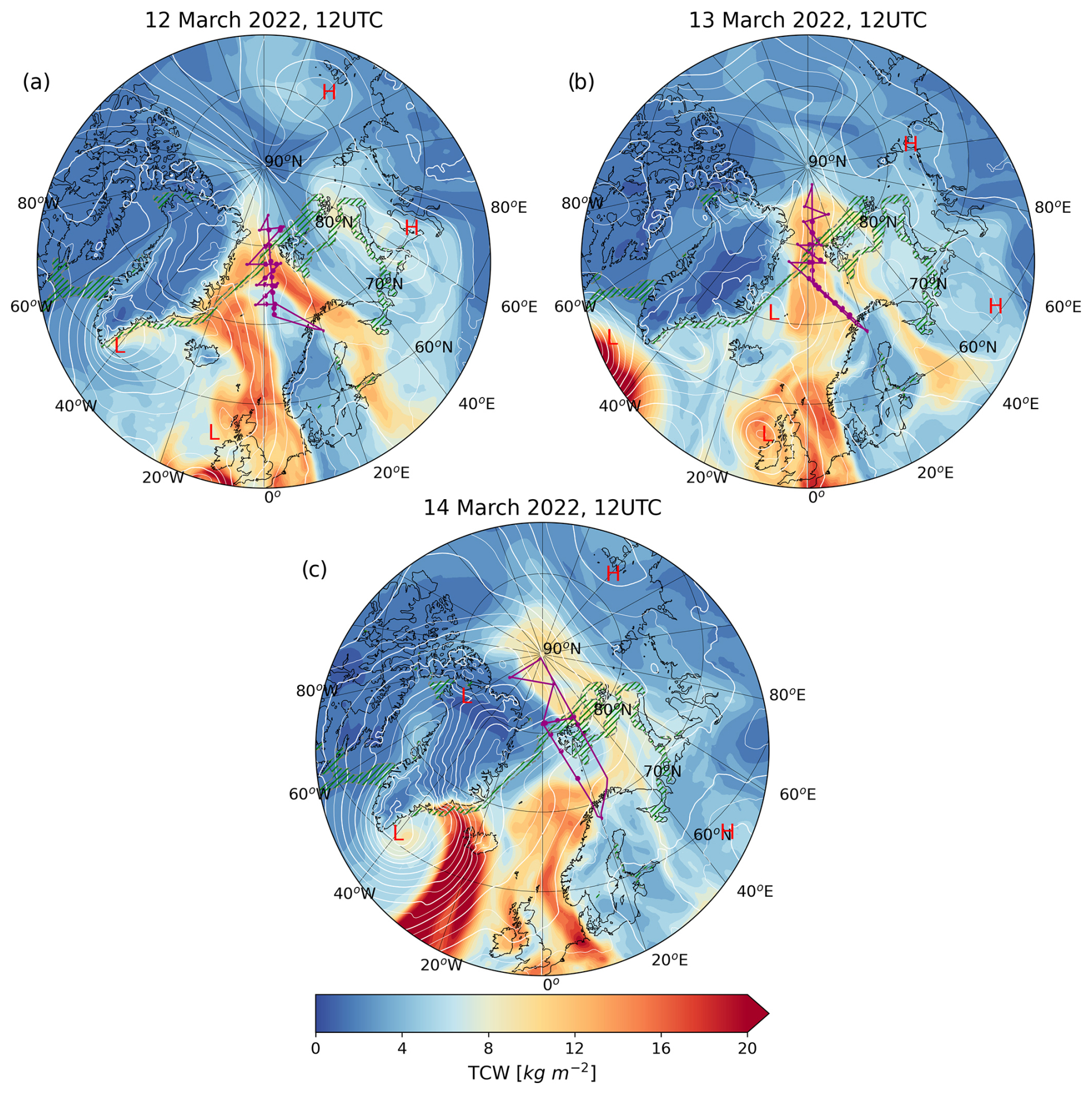
Figure 1 Maps of total column water (kg m⁻²) at 12:00 UTC on each day of the 12–14 March WAI event. Mean sea level pressure contours between 940 and 1080 hPa are plotted with thin (thick) white lines with a 5 (10) hPa step. The low- and high-pressure centers are marked with red letters. The green hatched area marks the extent of the marginal ice zone (MIZ), which corresponds to sea ice fraction values between 0.15 and 0.8. Purple lines represent the respective HALO flight tracks (RF02, RF03, RF04) over the North Atlantic. The purple dots correspond to the locations of dropsondes released during each flight.

During consecutive research flights RF02, RF03, and RF04 (Wendisch et al., 2024), a total of 50 Vaisala RD41 dropsondes (Vaisala, 2020) were released along the axis of the advection over the Fram Strait, covering a distance of approximately 10 latitudinal degrees (71–81° N). Detailed information on the dropsonde data can be found in Ehrlich et al. (2025). We use the dropsonde-derived vertical profiles of temperature, specific humidity, and horizontal wind, from approximately 12 km to the surface, to illustrate the observed Lagrangian evolution of the air mass and evaluate its representation in the model. For the evaluation of the modeled cloud properties, we use neural network retrievals of the cloud liquid water path (LWP) based on brightness temperature observations obtained with the HALO Microwave Package (HAMP, Mech et al., 2014). Retrievals are available only over the open ocean. To enable comparison we compute the medians over 15 min intervals; the original temporal resolution of the LWP time series temporal is 1 s.

2.2 Lagrangian trajectories

In order to approximate the advection path of the air mass, we use LAGRANTO (Sprenger and Wernli, 2015), a Lagrangian trajectory calculation and analysis tool, applied here to the three-dimensional ERA5 (Hersbach et al., 2020) wind field. ERA5 can be considered a reliable representation of the atmosphere (Graham et al., 2019) due to its global coverage, relatively high spatial and temporal resolution (here 0.25°×0.25° on the horizontal plane and 137 vertical levels on an hourly time step), and, lastly, the continuous assimilation of in situ and satellite observations within 12 h windows.

On 13 March at 12:00 UTC we launch 24 h long trajectories, 600 in total, half of which were computed backward and half forward in time. All trajectories are initialized within a 100 km radius from the center of the sampled area (81° N, 5° E, see Fig. 2a) at pressure levels 500, 600, 700, 800, 850, and 900 hPa (Fig. 2b). The initialization of the trajectories at this location guarantees more matches between trajectory and observational points, which enables the comparison. We assessed the stationarity of the synoptic flow by computing additional trajectories within a 2-hourly window around the selected initialization time, which showed negligible changes. We test whether the trajectories adhere to the same vertical alignment pattern suggested by Svensson et al. (2023) by searching for trajectories at different pressure levels that maintain the smallest relative distances (Fig. 2b). We consider this ensemble of aligned trajectories to be indicative of the air mass path and use it to simulate the Lagrangian air mass transformation.

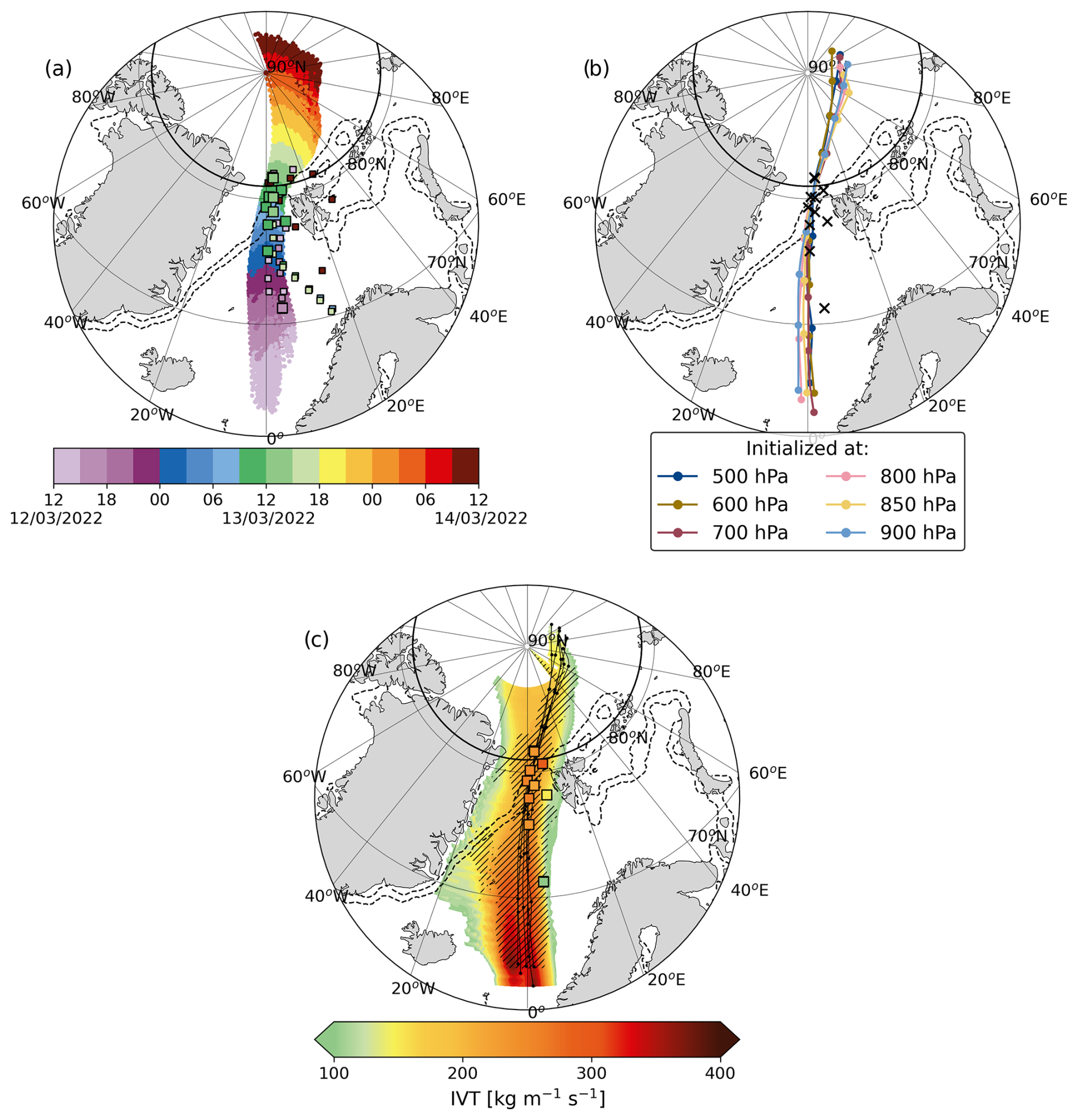
Figure 2 (a) 24 h long backward and forward trajectories initialized at pressure levels (500, 600, 700, 800, 850, and 900 hPa) within a 100 km radius circle centered on 81° N (marked with a thick solid line) and 5° E on 13 March at 12:00 UTC. The coloring along the trajectories represents the air parcels' time of arrival at the marked location. The squares mark the locations of all dropsondes released during flights RF02, RF03, and RF04 and are tinted, similarly to the trajectories, according to the dropsonde launch. Smaller squares are used to denote observations whose location and time of launch make them unfit for comparison with trajectories. Dashed contours show boundaries of the MIZ, corresponding to sea ice concentration values of 0.15 and 0.8, at the time of the trajectory initialization. (b) The trajectory ensemble showing the closest vertical alignment. Trajectories are colored according to the pressure they were initialized at. Dots mark 6 h long periods. X-shaped markers show the locations of observed profiles suitable for comparison. (c) Map of the temporal evolution and spatial variability of integrated water vapor transport (IVT). The trajectory ensemble, drawn with black lines, serves as a time axis. IVT changes in the direction parallel to the trajectories show the temporal evolution of the air mass. IVT changes in the direction perpendicular to the trajectories show the spatial variability of the air mass at the respective time step (12 March 2022 at 12:00 UTC at the southernmost point to 14 March 2022 at 12:00 UTC at the northernmost). Hatches mark the correlation range, showing areas around the trajectories of similar vertical structure at each time step (see Sect. 2.3).

At the point of initialization, 96 % of the total moisture content of the column is contained in the lowest 5 km. Therefore we consider the air mass transformation to be taking place within a 5 km deep layer above the surface and do not examine trajectories at lower pressure levels. Additionally, we do not seek vertical alignment in trajectories at pressure levels higher than 900 hPa that may fall within the boundary layer. This is due to the expectation that the friction-induced wind shear and veer (vertical gradients in wind speed and direction, respectively) near the surface would cause air parcels to move in different directions to the rest of the air mass. However, we also expect the interaction with the changing surface properties through vertical mixing to be driving changes in the boundary layer properties more strongly than any potential differential advection, leading us to treat the boundary layer as part of the advected air column.

2.3 Air mass detection

We provide an estimate of the WAI's spatial extent by following along the trajectory ensemble (Sect. 2.2) and, at each time step, scanning the neighboring ERA5 grid cells in the direction perpendicular to the mean flow to locate the edges of the advected air mass. These are identified using an integrated vapor transport (IVT) threshold of 100 $\mathrm{kg}{\mathrm{m}}^{-\mathrm{1}}{\mathrm{s}}^{-\mathrm{1}}$, generally preferred for Arctic WAI and AR detection (Gorodetskaya et al., 2014; Guan and Waliser, 2015; Woods et al., 2013; Viceto et al., 2022; Zhang et al., 2024). IVT values during the 12–14 March 2022 WAI event lie roughly between 120–220 $\mathrm{kg}{\mathrm{m}}^{-\mathrm{1}}{\mathrm{s}}^{-\mathrm{1}}$ (Walbröl et al., 2024), making 100 $\mathrm{kg}{\mathrm{m}}^{-\mathrm{1}}{\mathrm{s}}^{-\mathrm{1}}$ appropriate for the air mass detection. We compute the total IVT as the vector sum of the meridional and zonal components, derived from ERA5, to account for potential changes in the direction of transport from mainly meridional to zonal as the air mass crosses the Arctic (Fig. 2b and c).

Information on the extent of the air mass is necessary for determining its internal spatiotemporal variability and understanding the different transformation pathways that can be encountered within it. Within the margins of the moist plume, we look for profiles of temperature, humidity, wind speed, and cloud liquid and ice water content of similar structure to the profiles on the trajectories. Correlation is examined only within the lowest 3 km, where variability is expected to be larger, and is assessed using the Pearson correlation coefficient. The correlation range (P_co>0.5) marks the extent of what could be considered a column-like air mass that is uniformly transformed along the trajectory ensemble (Fig. 2c). In contrast, the parts of the plume that fall outside the correlation range are air masses whose evolution cannot be represented by the selected trajectory ensemble.

2.4 Model description and Lagrangian simulations

The Atmosphere–Ocean Single Column Model (AOSCM, Hartung et al., 2018) follows the development version of EC-Earth (Döscher et al., 2022) in a 1D framework. In the AOSCM, the SCM version of the atmospheric model OpenIFS cy43r3 (Open Integrated Forecasting System; https://confluence.ecmwf.int/display/OIFS/About+OpenIFS, last access: 26 November 2024) is coupled to a column of the ocean model NEMO3.6 (Nucleus for European Modelling of the Ocean; https://www.nemo-ocean.eu/, last access: 26 November 2024) through the OASIS3-MCT coupler (https://oasis.cerfacs.fr, last access: 26 November 2024). The parameterization schemes for radiation, turbulence, convection, and cloud microphysics are described in detail in the IFS cy43r3 documentation (ECMWF, 2017). Sea ice processes in NEMO are represented by LIM3 (Rousset et al., 2015). In our setup, five thickness categories and two vertical levels were used to describe the sea ice, while snow is represented by a singular layer on top of the sea ice. The LIM3 halo-thermodynamic parameterizations are solved for all categories and levels. In an Eulerian framework, information on the large-scale flow is easily introduced into the model through the prescribed forcing. The model uses ERA5 vertical velocity profiles (ω) to include the effect of large-scale divergence and geostrophic wind profiles for the application of a pressure gradient forcing on the column, while advection of heat, moisture, cloud water, and momentum is represented with the introduction of an advective tendency term in the state variables' prognostic equations. A detailed guide for designing and executing AOSCM experiments is given in Hartung et al. (2018, 2022).

For Lagrangian applications, the AOSCM requires information on the air mass path, which, in our case, is indicated by the vertically aligned trajectory ensemble (Sect. 2.2). The atmospheric column is made aware of its poleward advection through the temporally varying surface conditions and large-scale dynamical forcing, the details of which (surface type, surface temperature, and large-scale subsidence) are obtained from ERA5 reanalysis data along the predesignated air mass tracks. The along-stream conditions may slightly vary between the individual trajectories, despite the spatial and temporal proximity within the ensemble. Therefore, we use all initial profiles paired with their respective along-stream surface and dynamic conditions to perform ensemble simulations. This approach gives some insight on the mean characteristics of the air mass transformation but also reveals its sensitivity to potential variability in initial conditions and forcing factors.

We set the advective tendencies to zero, inhibiting the inflow (outflow) of heat, moisture, or momentum from (to) the ambient atmosphere. Pressure gradient forcing leads to the emergence of inertial oscillations close to the surface, which lead to unphysical surface fluxes of heat and momentum. In order to suppress these spurious oscillations we nudge the horizontal wind to the ERA5 profiles throughout the entire column and set the nudging timescale (τ_nudge) to be equal to the model time step (15 min).

The sharp changes in surface properties require the division of each trajectory into three legs: ocean, marginal ice zone, and sea ice. The air mass spends approximately 21, 3, and 25 h over each leg, traveling 1500, 145, and 1218 km distances, respectively. Over ocean, the inclusion of the sea surface temperature (SST) meridional gradient is crucial, whereas the two-way sea–atmosphere interaction is less relevant, considering the high speed of advection. The standalone atmospheric model is therefore more well-suited for this part of the simulation since it allows for the prescription of the SST evolution.

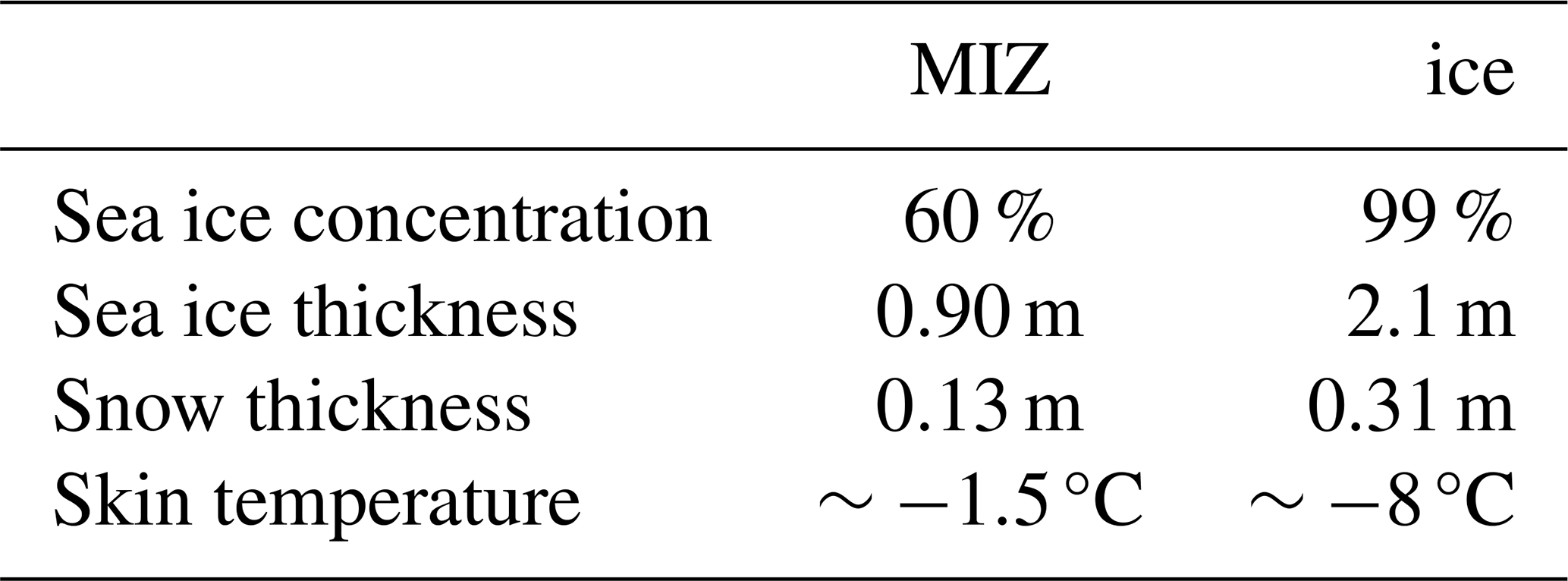
As the air mass flows over the marginal ice zone (MIZ, sea ice fraction >0.15 and <0.8), the crude treatment of sea ice in OpenIFS becomes increasingly problematic, making the coupled configuration more suitable. In coupled mode, the AOSCM allows for a more realistic representation of the sea ice thickness and grid-scale variability. Additionally, the use of the sea ice model LIM3 allows the presence of snow on ice, which has been shown to mitigate surface energy and near-surface air temperature biases (Pithan et al., 2016). The start of the third and final leg is marked by the sea ice fraction increase above 0.8. The sea ice model for both legs is initialized using ERA5 information for the sea ice area concentration. We initialize the sea ice at lower temperatures than indicated by reanalysis. This causes the downward conductive heat flux to counterbalance the incoming energy, maintaining a colder skin temperature, comparable to the respective mean ERA5 values for each leg (Fig. B1f and Table 1). As a result, the surface fluxes are closer to ERA5 (Fig. B1a–e). The thickness of the sea ice and snow layers as well as profiles of the oceanic temperature, salinity, and currents are obtained from the CMEMS Global Ocean Physics reanalysis dataset (https://doi.org/10.48670/moi-00016). Reference values for the sea ice conditions in each leg are given in Table 1.

Table 1 Representative values for sea ice and snow properties used in the coupled simulations.

The modeled profiles at the final time step of the previous simulation were used as initial conditions for the following simulation at each transition point between surface regimes. Two additional preparatory simulations are performed over each sea ice leg. The first one used the standalone OpenIFS model to produce a first estimate of the surface energy fluxes needed for the ice model at the first time step, and the second one used the coupled model for a 2 h long simulation, in order to reach a sea ice state that is more in balance with the atmosphere. This helps mitigate abrupt spikes in the surface energy fluxes at the beginning of the third simulation leg.

3 Results and discussion

3.1 Large-scale setting and air mass transport

On 12 March 2022, a low-pressure system developed over the southeast coast of Greenland and a strong high-pressure system extended over Scandinavia (Walbröl et al., 2024), creating a meridional path for the warm and moist midlatitude air to enter the Arctic (Fig. 1a). From a climatological perspective, this dipole flow configuration over the North Atlantic is the most common driver of Arctic moist intrusions, responsible for about 75 % of the events (Papritz et al., 2022). Despite the Greenland low weakening, meridional advection persists through 13 March (Fig. 1b), sustained by the development of a new low, west of the UK. On 14 March (Fig. 1c), the south Greenland low deepens once again, due to the arrival of a strong cyclone from the southwest, and connects with a smaller cyclone forming over north Greenland. This configuration causes the isobars to curve and displaces the flow to the east as the air mass approaches the North Pole. This extensive low-pressure system stretching over Greenland, in combination with the persistent Scandinavian blocking, sets up for yet another WAI into the Arctic in the following days (Walbröl et al., 2024).

Trajectories initialized over the MIZ at different pressure levels within the advection layer show the path of the air mass (Fig. 2a). The moist air mass flows over the Atlantic, along the 0° meridian for 24 h, reaching the MIZ at around 10:00 UTC on 13 March and the central Arctic around 24 h later. The trajectories slowly spread out on both ends, with their maximum in-between distance ranging from 200 km over the MIZ (the diameter of the circle within which they were initialized) to around 700 km (Fig. 2a). Within this large suite of trajectories, we find a smaller subset, comprised of one trajectory per pressure level. The trajectories in this subset exhibit a considerably narrower spread (260 km at the point of maximum divergence), thus appearing roughly vertically aligned (Fig. 2b).

Vertical alignment within parcels traveling at different heights suggests that the air mass maintains a consistent column-like structure throughout its 49 h journey into the Arctic. We examine whether the advection and transformation of the air masses around the trajectories are similar enough for them to be likened to a cohesive atmospheric column. The trajectory ensemble runs through the narrow center of the meridional transport corridor where IVT values are the highest (around 350 $\mathrm{kg}{\mathrm{m}}^{-\mathrm{1}}{\mathrm{s}}^{-\mathrm{1}}$ in the southernmost end to approximately 150 $\mathrm{kg}{\mathrm{m}}^{-\mathrm{1}}{\mathrm{s}}^{-\mathrm{1}}$ near the North Pole, Fig. 2c). The correlation range (hatched section), which envelops columns of similar vertical structure (see Sect. 2.3), becomes thinner with time but consistently encompasses the entire trajectory ensemble. In simpler terms, the flow within a certain distance from the trajectories is relatively uniform in both IVT and vertical structure. Therefore, our trajectory ensemble is narrow enough to be regarded as representative of a single air column that is advected and transformed in a coherent way.

Vertical alignment in Arctic WAIs has also been encountered in past studies (Ali and Pithan, 2020; Svensson et al., 2023), although further investigation is needed in order to determine how common it is among WAIs. Nevertheless, when this feature is encountered, it facilitates the exploration of Arctic air mass transformations with simple 1D models such as the AOSCM. The framework can be applied to more WAI case studies and the results can be used to evaluate and build on our theoretical understanding of such events (Pithan et al., 2018).

3.2 Spatial variability of air mass transformation in ERA5

The along-stream transformation of the air mass is shown in Fig. 3 in terms of integrated column water (vapor, liquid and ice) (Fig. 3a–c) and surface energy budget (SEB) terms (Fig. 3d–i). The integrated water vapor (IWV) content of the air mass is initially rather high, 16 kg m⁻² on average (Fig. 3a), and decreases as the air mass advances northward, slowly over the ocean but more rapidly over ice, to about half of the initial value. The majority of the moisture is gathered towards the center of the air mass (0° longitude over the ocean where the spatial gradient is more evident) and decreasing towards the edges, while the spatial extent of the air mass also varies along the advection path. The western sector of the air mass is more susceptible to the synoptic systems developing over Greenland (Fig. 1), which explains the occasional westward divergence of the moisture (e.g., westward spread towards the Greenland coast at around 70° N, as well as later on, north of Svalbard).

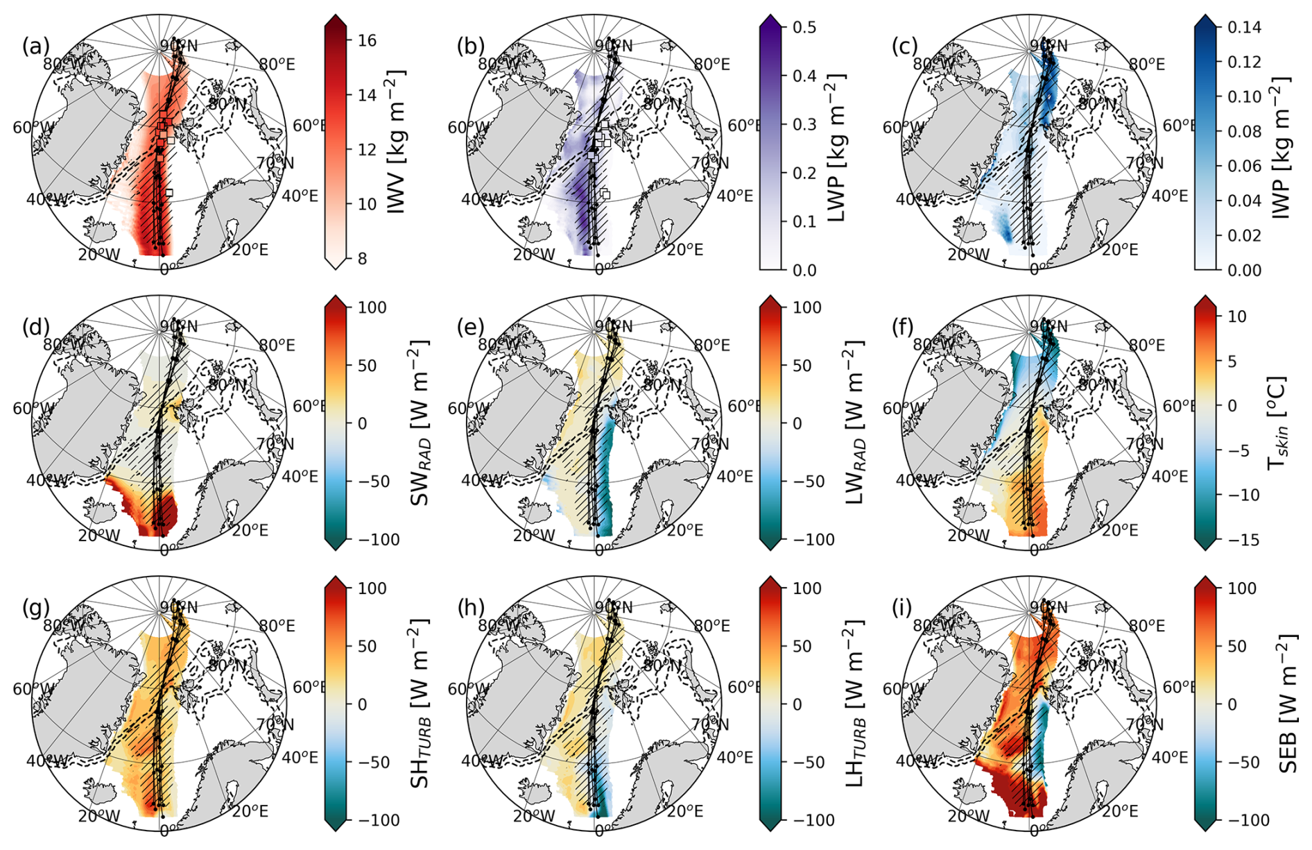
Figure 3 Temporal evolution and spatial variability of the air mass during its poleward advection in terms of integrated specific water content of vapor, liquid, and ice cloud (a–c) and energy exchange at the surface (d–i). Fluxes are positive towards the surface. The trajectory ensemble, drawn with black lines, serves as a time axis, similar to Fig. 2c. Hatches mark the correlation range (see Sect. 2.3) around the air mass at each time step. Square markers, when present, correspond to the observed values. Dashed contours show boundaries of the MIZ, corresponding to sea ice concentration values of 0.15 and 0.8 on 13 March at 12:00 UTC.

Measurements conducted within 250 km and 3 h of a trajectory point are considered suitable for comparison (11 out of 50 dropsondes). The dropsonde profiles included in the correlation range are in general agreement with the ERA5 IWV content, although appearing slightly drier over the ocean and moister over the MIZ (Fig. 3a). The profiles located on the eastern boundary of the air mass show a consistent mismatch with ERA5 data, in most cases severely lacking in moisture content. Observations from these research flights were not submitted to the Global Telecommunication System (GTS) for assimilation (Ehrlich et al., 2025), which explains why the observed steep moisture gradient at the air mass boundary is not represented in ERA5.

The spatial variability is even more prominent in the cloud liquid water path (LWP, Fig. 3b) fields, with most of the cloud liquid water found west of the prime meridian for the time the air mass spends over the ocean. The LWP is abruptly depleted as the air mass crosses the MIZ and remains small all the way into the central Arctic. The observed spatiotemporal cloud distribution is similar to ERA5. ERA5 shows a positive LWP bias (−0.03 kg m⁻² on average) in the east sector of the air mass, where the cloud is thin, and a negative LWP bias (−0.04 kg m⁻² on average) in the west where thicker clouds are encountered. The biases are larger than the estimated uncertainty of the LWP retrieval (0.02 kg m⁻²). The depletion of the liquid cloud over the MIZ is concurrent with an increase in the ice water path (IWP, Fig. 3c). The glaciation of the cloud is visibly accelerated at higher latitudes, near the northernmost end of the trajectories.

The net shortwave radiation along the path of the air mass is presented in Fig. 3d. At the time of the event (12–14 March), the Arctic receives roughly 7–11.4 h of daylight depending on the latitude of interest. Therefore, solar radiation is only relevant for small parts of the air mass transformation. The surface shortwave radiative flux is largest near the south end of the trajectories (∼200 W m⁻²). Its spatial distribution mimics that of the liquid cloud water within the air mass (Fig. 3b). On the western flank of the air mass, where the LWP is larger, the liquid cloud blocks approximately up to 300 W m⁻² of solar radiation (Fig. A1a). In contrast, the liquid cloud consistently casts a longwave radiative forcing of around 80 W m⁻² (Fig. A1b), which changes the sign of the net surface longwave flux to positive (Fig. 3e). In the eastern sector, the weaker cloud presence is not able to compensate for the upwelling longwave radiation emitted by the warmer surface (Fig. 3f), yielding a negative radiative balance (Fig. 3e). Once the air mass flows over sea ice, the longwave radiation becomes a consistent net source of energy for the surface.

Despite the large meridional skin temperature gradient – more than 20 °C (Fig. 3f) between southernmost and northernmost end of the trajectory ensemble – the air mass is consistently warmer than the surface, losing energy to it through the turbulent sensible heat flux throughout its Arctic journey (Fig. 3g). The spatial variability in skin temperature over the ocean also appears to be controlling the exchange of latent heat at the surface (Fig. 3h). Over the warm ocean, the strongly negative (upward) fluxes indicate ongoing moisture uptake by the air mass. Over colder waters, the latent heat fluxes turn positive (downward) and are of similar magnitude as over the sea-ice-covered surface, implying persistent water vapor deposition from the air mass onto the oceanic surface.

The sum of the all radiative and turbulent surface fluxes yields the surface energy budget (SEB) depicted in Fig. 3i. Along the trajectories, the surface receives the most energy within the first few hours, largely due to the contribution of the solar radiation. However, in the absence of solar radiation, the SEB shows a strong zonal gradient over the ocean. Two distinct regimes can be identified. In the positive SEB regime (western sector of the air mass), energy is transferred from the air mass to the surface (∼50 W m⁻²) through both longwave radiation and turbulent heat exchange. In the negative SEB regime ($\sim -$50 W m⁻²) on the eastern side, the ocean temperatures are high and the liquid cloud cover is low, causing the upward latent heat and longwave radiation to outweigh the downwelling sensible heat flux. Our trajectory ensemble runs between the two regimes, favoring the negative regime for the first 10–12 h and crossing through to the positive regime from then onwards. Entering the MIZ, the SEB becomes uniformly positive across the air mass. Most of the energy received by the surface (∼60 W m⁻²) is contributed by turbulent heat fluxes. Farther into the Arctic, the SEB reaches 75 W m⁻², with mainly the sensible heat flux and, to a lesser degree, the latent heat and the downward emitted longwave radiation counteracting the surface radiative cooling. The timeline of the SEB during the intrusion shows the strong impact on the Arctic system, as well as the effect of the surface forcing on the air mass transformation.

3.3 Modeling the air mass transformation

We have established that the vertical alignment of the trajectories within the advection layer gives merit to the simplified view of the intruding air mass as an atmospheric column and justifies the application of the AOSCM for the study of the air mass transformation.

In our AOSCM ensemble simulations (Sect. 2.4), we use the mean temperature of the lowest 5 km (${\stackrel{\mathrm{‾}}{T}}_{\mathrm{5}\mathrm{km}}$) and the vertically integrated water vapor content over the same layer (IWV_5 km) as indices for the heat and moisture content of the air mass, respectively (Fig. 4). The relative evolution of these two variables enables identification of potential heat and moisture sources/sinks and their effective timescales for the air mass transformation along the trajectories. Along with the AOSCM simulations we also present ERA5 and IFS Cy47r3 operational forecast data (IFS-OF) in order to test the consistency in the results between the Lagrangian and Eulerian modeling approaches. Finally, the dropsonde observations collected along the air mass path are synthesized to demonstrate the observed Lagrangian evolution of the air mass heat and moisture.

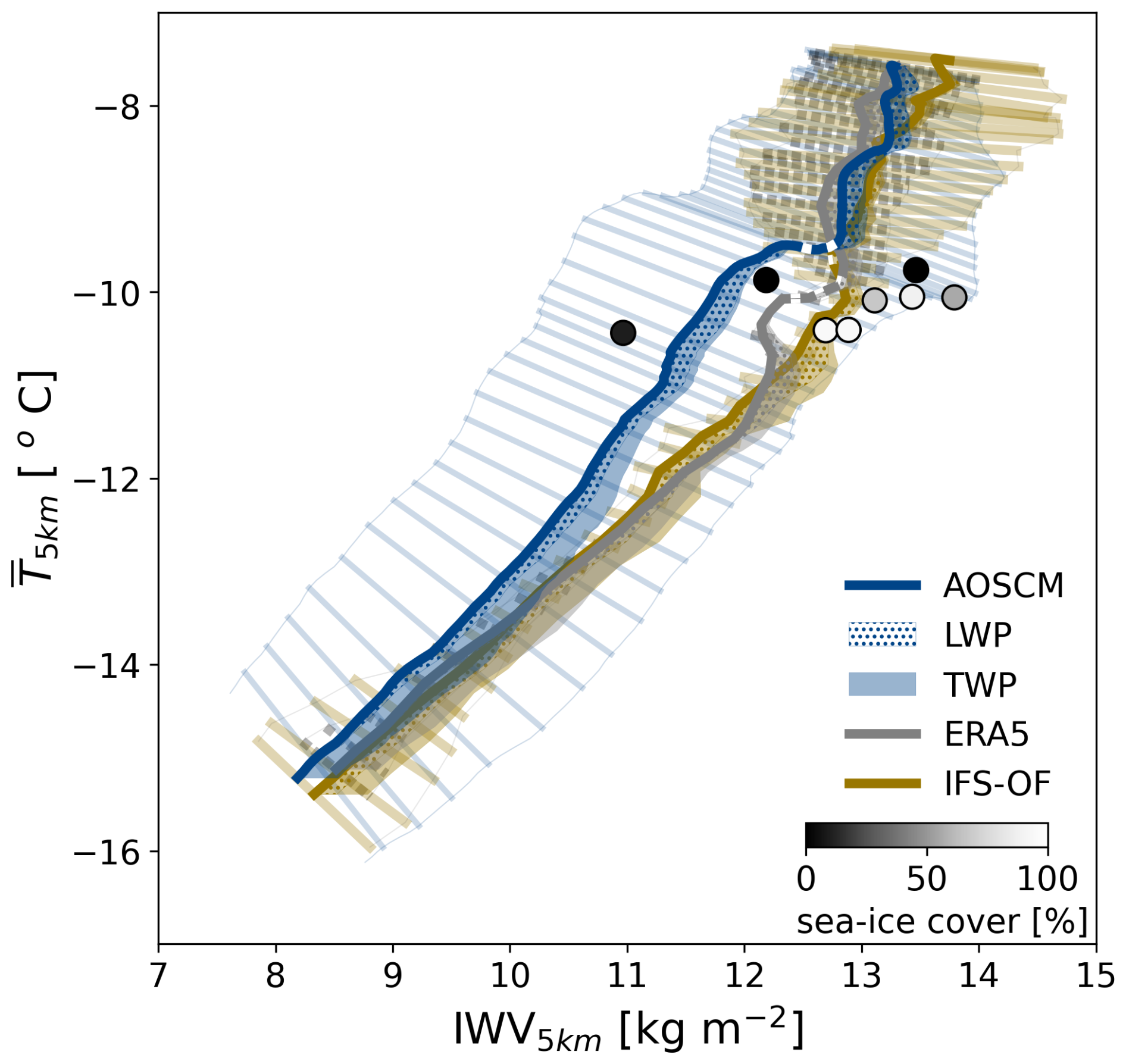
Figure 4 Mean air mass temperature (${\stackrel{\mathrm{‾}}{T}}_{\mathrm{5}\mathrm{km}}$, °C) and water vapor content (IWV_5 km, kg m⁻²) along the advection path for AOSCM simulations (blue), ERA5 (gray), and IFS-OF data (sand). Drawing the MIZ with a dashed line helps distinguish the sections of the air mass transformation taking place over different surface types. The length of the faded lines crossing the mean curves shows the ensemble standard deviation, while their slope shows the ratio of the individual components (temperature and moisture content). The faded lines are plotted with a time step of 1 h, and therefore their density signifies the speed of the transformation. The width of the shaded areas attached to the right of the thick solid lines represents the vertically integrated total water path (TWP). Dots are used to show the portion that is in liquid phase (LWP). Observations are shown with circular markers, shaded according to the sea ice fraction of the closest ERA5 column at sampling time.

3.3.1 Transformation over the ocean

The initial state of the air mass is depicted in the top right corner of Fig. 4. Since the AOSCM is initialized with ERA5 data, the initial state between the two products is identical (13.3 kg m⁻² and −7.6 °C). IFS-OF shows a slightly colder and moister air mass at around −7.7 °C and 13.8 kg m⁻², respectively. The curves display a steep slope during the advection over ocean, more prominent in ERA5 and AOSCM, indicating a faster loss of heat over moisture. The total cloud water content of the air mass, liquid in its majority, evolves similarly to the moisture. The overall changes sum up to approximately −2 °C for temperature and a mere −0.5 kg m⁻² for moisture, on average, for the AOSCM and ERA5. For IFS-OF the respective changes are −2 °C and −1 kg m⁻².

The standard deviation is shown with faded lines perpendicular to the main curves and depicts the variability. At the southernmost point of the air mass, all products agree on a standard deviation of approximately 0.7 kg m⁻² for IWV and 0.1 °C for temperature. The variability around the curves drops for ERA5 and IFS-OF due to the trajectories converging when approaching the MIZ, while for the AOSCM it expands, showing an increase of 0.3 kg m⁻² and 0.5 °C for moisture and temperature, respectively. The increase in the AOSCM ensemble uncertainty is the combined result of the variability in the ensemble's initial conditions and along-stream forcing. The slight tilt in the faded perpendicular lines shows the uncertainty in the predicted air mass heat content growing with simulation time.

Observations over the ocean (black dots) show a large scatter, especially in IWV_5 km. The AOSCM uncertainty range is wide enough to encompass the observed variability. It should be noted that the observational data points presented in Fig. 4 do not include the dropsondes released close to the edge of the moist air mass (71° N, 4° E and 78° N, 7° E in Fig. 3a) and are, expectedly, not representative of its evolution.

3.3.2 Transformation over the MIZ

Over the MIZ (denoted with dashed lines in Fig. 4), there is a distinct change in the evolution of the air mass showcased by all considered products. The slope of the curves becomes flatter, pointing to the more rapid loss of moisture and a comparatively slower decrease in the heat content. The AOSCM shows a 0.5 kg m⁻² drop in IWV_5 km but no significant cooling. The standard deviation remains mostly unchanged. The ERA5 curve exhibits a similar flattening, showing a moisture loss similar to the one predicted by AOSCM (0.5 kg m⁻²) but a slightly more pronounced cooling (∼0.2 °C). The IFS-OF shows a less severe change in slope, with the moisture and temperature content changes of the same order as over the ocean. However, it is important to note that the residence time of the air mass over ocean and MIZ is substantially larger. In that context, the weakening of the air mass cooling is more modest, while the acceleration of the moisture depletion is striking. Observations over the MIZ show a similar ${\stackrel{\mathrm{‾}}{T}}_{\mathrm{5}\mathrm{km}}\sim {\text{IWV}}_{\mathrm{5}\mathrm{km}}$ trend, agreeing with the timescales of heat and moisture loss but displaying higher absolute IWV values as large as 1 kg m⁻² compared to AOSCM and ERA5. The IFS-OF curve is, interestingly, in closer agreement with the observed values.

3.3.3 Transformation over sea ice

The most drastic part of the transformation takes place over sea ice (Fig. 4). For the AOSCM, the slope of the curve becomes steeper again, indicating the loss of both heat and moisture at a much faster rate. Cooling is slightly stronger in the first half of the sea ice leg and slows down again towards the end, with moisture loss being more dominant. At the same time, the total cloud water content grows and gradually converts from liquid to ice by the end of the simulation. ERA5 appears to be lagging behind in moisture loss at the beginning of the sea ice leg compared to the AOSCM simulations, while, in contrast, IFS-OF dries more rapidly through the entire leg. However, all products show strong agreement on the final state of heat and moisture content, as well as total cloud water path. While the cloud in AOSCM and ERA5 has become almost entirely glaciated by the end of the transformation, around 50 % of the cloud water in IFS-OF is still in liquid phase.

The uncertainty ranges around the ERA5 and IFS-OF curves grow larger due to the slight divergence of the trajectory ensemble. In contrast, the uncertainty range for the AOSCM appears to be narrowing down again to its initial value (0.7 kg m⁻²) for IWV_5 km, but it is an order of magnitude larger for ${\stackrel{\mathrm{‾}}{T}}_{\mathrm{5}\mathrm{km}}$ compared to the initial state (almost 1 °C), comparable to the range of IFS-OF. The upward tilt of the perpendicular lines indicates greater variability in heat compared to moisture content, in contrast to the beginning of the simulation when the opposite was true. This feature is more pronounced in the AOSCM simulations but also apparent in ERA5 and IFS-OF. The similarities among the different products in the evolution of the air mass mean properties and variability suggest that the AOSCM, if appropriately forced, is able to represent the physical processes that drive the air mass transformation.

AOSCM, ERA5, IFS-OF, and observations all show a similar evolution of heat and moisture content. Similarities between ERA5 and AOSCM are less surprising since ERA5 data were used for initialization and forcing of the AOSCM. However, the AOSCM is also able to reproduce an air mass transformation of magnitude and timescales comparable to its 3D counterpart, IFS-OF. The observed air mass transformation, to some extent, displays similar features. However, comparison is hindered by the large scatter of observations and their confinement within a small area around the MIZ. Several factors could be contributing to this scatter. These include (i) the spatial inhomogeneity of the air mass properties that is not entirely represented by our small trajectory ensemble, (ii) the relative horizontal displacement of the dropsondes during their descent (some of them could be landing closer to or in the MIZ), and, (iii) in some cases, the time intervals between measurements in the same area being large enough to allow changes related to advection.

3.3.4 Vertical structure

The transformative physical processes often act in different layers within the atmosphere. Therefore, in addition to the bulk changes in the mean or integrated air mass properties, changes in the vertical structure of the air mass also need to be considered in order to draw a comprehensive picture of the air mass transformation.

Our initial air mass appears to be warm and moist, primarily within the boundary layer, which reaches a depth of just over 1 km on average (Fig. 5a), but also above it, extending up to around 3 km. The boundary layer is diagnosed in the model as the layer adjacent to the surface within which the bulk Richardson number is below the critical threshold (Ri_c=0.25). The ensemble variability in the boundary layer depth estimate is overall small (∼30 m) except for the first 8 h of the simulation when it reaches up to 100 m. The boundary layer remains stably stratified throughout the simulation (Fig. 5d), with the air within the boundary layer constantly losing heat to the surface. The near-surface cooling intensifies as the air mass flows over the MIZ with a surface inversion starting to develop and the boundary layer becoming shallower. As the air mass moves past the MIZ and over fuller sea ice cover, the cooling extends through a deeper column within the atmosphere. Cooling aloft (1–5 km) weakens the surface inversion and leads to a slight boundary layer deepening by the end of the simulation. The uncertainty of the predicted thermodynamic structure, in terms of ensemble standard deviation, grows with simulation time. The largest values are encountered over sea ice between 1–4 km of altitude and are seemingly related to ensemble variability in the simulated cloud height and overall presence.

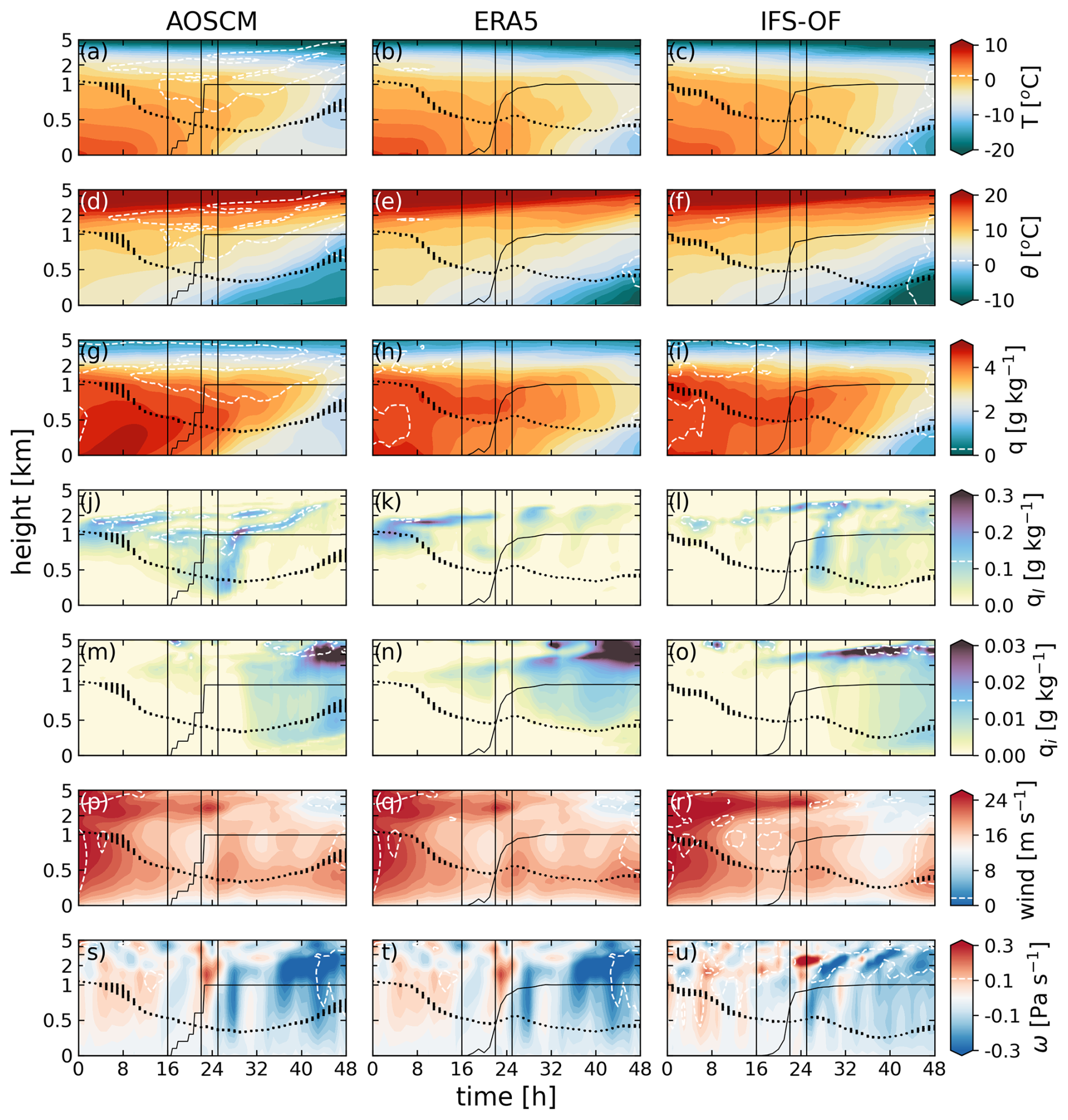
Figure 5 Time–height cross-sections of the ensemble average (a–c) temperature, (d–f) potential temperature (°C), (g–i) specific humidity (g kg⁻¹), (j–l) specific liquid content, (m–o) ice water content (g kg⁻¹), and (p–r) horizontal and (s–u) vertical wind speed (m s⁻¹) along the trajectories in the AOSCM simulations (left column), ERA5 (middle column), and IFS-OF data (right column). The time axis is in hours since 12 March 2022 at 12:00 UTC. The height axis is linear below 1 km and logarithmic above. The grayscale dashed contours show the ensemble standard deviation; contour intervals are marked on the respective color bars. The dotted line marks the ensemble mean PBL height, and the sizes of the dot markers represent the ensemble deviation. The black solid line shows the along-stream sea ice concentration.

Most of the moisture is contained in the lowest 2 km (Fig. 5g), suggesting a recent uptake over the North Atlantic, a common source region of moist intrusions according to Papritz et al. (2022). Despite the constant decline in the near-surface temperature through turbulent processes, the air mass takes up moisture from the surface during the first 12 h of the simulation. From around 12 h and onwards, while still over the ocean, the latent heat fluxes turn negative and the boundary layer is slowly depleted of its moisture, while the drying is accelerated as the air mass enters the MIZ and progresses farther into the Arctic.

The cloud in the AOSCM simulations initially consists of a single, solely liquid cloud layer at 1 km over the ocean surface, right on top of the boundary layer, which remains stable throughout the simulation (Fig. 5j). The cloud deck splits into two layers at around t=12 h and later, over the MIZ, a third liquid cloud layer is formed within the boundary layer. Finally, moving over higher sea ice concentrations, the cloud starts rising from the surface (Fig. 5j). The first signs of cloud glaciation appear as a response to cloud-top radiative cooling with ice clouds emerging at higher altitudes at the end of the ocean leg (Fig. 5m). Later on, the cloud specific ice water content increases at the expense of the cloud liquid due to the upward rise of the cloud and the accompanying adiabatic cooling (Fig. 5s).

The wind is initially strong, exceeding 25 m s⁻¹ at higher altitudes but also near the top of the boundary layer in what appears to be a low-level jet (Fig. 5p). The air mass gradually loses momentum throughout the column. When it reaches the MIZ, the additional surface-induced friction causes an additional deceleration on the wind within the PBL. Later in the simulation, over higher sea ice concentrations, the near-surface wind speed increases again in a jet-like structure around 0.5 km, while the wind in the overlying layers slows down.

In terms of the vertical wind, ω (Fig. 5s) is weak over the ocean, with the sign often alternating over the height of around 2 km. The vertical wind divergence within the liquid cloud is partially causing the cloud layer to split (Fig. 5j). Over the MIZ, the subsidence spikes abruptly and over the sea ice leg the vertical motion is predominantly upward, with ω increasing the deeper the air mass intrudes into the Arctic. The strong large-scale updraft in the AOSCM simulations and ERA5 data (Fig. 5s and t) coincides with the cloud water phase transition from liquid to ice (Fig. 5j, k, m, and n at t≃27 h), which is due to the induced adiabatic cooling. The ensemble ω standard deviation is also rather large, within the range of (0.05, 0.25] Pa s⁻¹, almost as large as the signal itself. Deviations of that magnitude have been shown to have a considerable impact on the evolution of the cloud layer Mirocha and Kosović, 2010; Neggers, 2015; Young et al., 2018; van Der Linden et al., 2019.

ERA5 and the IFS-OF (Fig. 5 middle and right columns) show a similar air mass transformation timeline as that simulated by AOSCM (Fig. 5 left column). The strengthening of the boundary layer stability is slightly delayed in ERA5 and the IFS-OF (Fig. 5e and f), presumably because of differences in the treatment of snow/sea ice and atmosphere coupling between AOSCM and the two 3D products. OpenIFS, the model responsible for the production of both IFS-OF and – in part – ERA5 data, uses a sea ice layer of fixed thickness (1.5 m), entirely disregarding the presence of snow on top of sea ice, while the AOSCM is only set up to reproduce the bulk changes in the sea ice surface temperature (see Sect. 2.4), therefore potentially misrepresenting their timing. By the end of the trajectories, however, the ERA5 and IFS-OF inversion grows stronger than what the AOSCM is able to simulate, resulting in a shallower boundary layer in comparison. Additionally, the boundary layer over the ocean is drier in ERA5 and IFS-OF (Fig. 5h and i); the near-surface specific humidity remains constant for the first 8 h of the transformation before decreasing. The ensemble standard deviation for all ERA5 and IFS-OF variables is maximum at the start and the end of the transformation, decreasing over the MIZ, at around 24 h, when the trajectories converge and therefore cross fewer grid points.

The ERA5 liquid and ice cloud structure (Fig. 5k–n) matches the AOSCM's (Fig. 5j–m), more so over the ocean than over the sea ice, showing a similar split of the cloud layer over the MIZ and comparable timescales for the cloud water phase transition. The cloud in IFS-OF bears less resemblance to AOSCM than to ERA5, especially over the ocean where the cloud exhibits discontinuities and smaller liquid water content (Fig. 5l) and over sea ice where the IFS-OF specific ice content is notably smaller (Fig. 5o). However, the multilayer liquid cloud structure over the MIZ and early sea ice leg is found in all three products.

The use of ERA5 data for forcing the AOSCM is partly the reason behind the stark similarities between the two products. The strong wind nudging (τ=900 s) and prescribed vertical velocities (ω), explaining the identical appearance of Fig. 5p, q, s, and t, respectively, influence the changes in the thermodynamic and cloud structure of the air mass. The larger differences between IFS-OF and AOSCM are, therefore, to be expected, especially when considering that the trajectories, along which we study the air mass transformation, were computed on ERA5 data. This is evident in the stronger IFS-OF baroclinic wind shear over the ocean and MIZ compared to ERA5 (Fig. 5q and r), which could lead to a different air mass path and a smaller degree of vertical alignment between the trajectories. The vertical velocity ω is also different in IFS-OF, exhibiting larger temporal and spatial variability in both the mean signal and the ensemble standard deviation (Fig. 5u).

3.3.5 Comparison with observed transformation

We synthesize the dropsonde profiles of temperature and moisture taken along the air mass path to evaluate whether the modeled and observed air mass transformations exhibit the same features and timescales (Fig. 6). The majority of observations suitable for comparison are gathered around the MIZ area (Fig. 2). To make the comparison more convenient, we cluster the measured profiles according to the surface type they are conducted over: ocean (Fig. 6a–e), MIZ (Fig. 6f–j), and sea ice (Fig. 6k–o). For the clustering we use the ERA5 sea ice concentration of the nearest grid at the time closest to the dropsonde launch. The ensemble mean AOSCM, ERA5, and IFS-OF profiles are taken in the center of each dropsonde cluster. Over the ocean, observations show a temperature profile similar to AOSCM, ERA5, and the IFS-OF, with the exception of a layer between 2–4 km that appears to be generally cooler in the dropsonde measurements (Fig. 6a). Over the MIZ, the observed air temperature near the surface is slightly positive, approaching zero, which is consistent with the AOSCM, as well as ERA5 and IFS-OF (Fig. 6f). Dropsondes released over full sea ice cover demonstrate a smaller surface cooling compared to the AOSCM ensemble mean (Fig. 6k). In the AOSCM, the near-surface temperature and specific humidity drop by approximately 4 °C (Fig. 6k and m) as a response to the enforced decrease in skin temperature (see Table 1 and Fig. B1). ERA5 and especially IFS-OF match the observed thermodynamic structure near the surface, while all products (including the AOSCM) are in agreement with observations over 500 m.

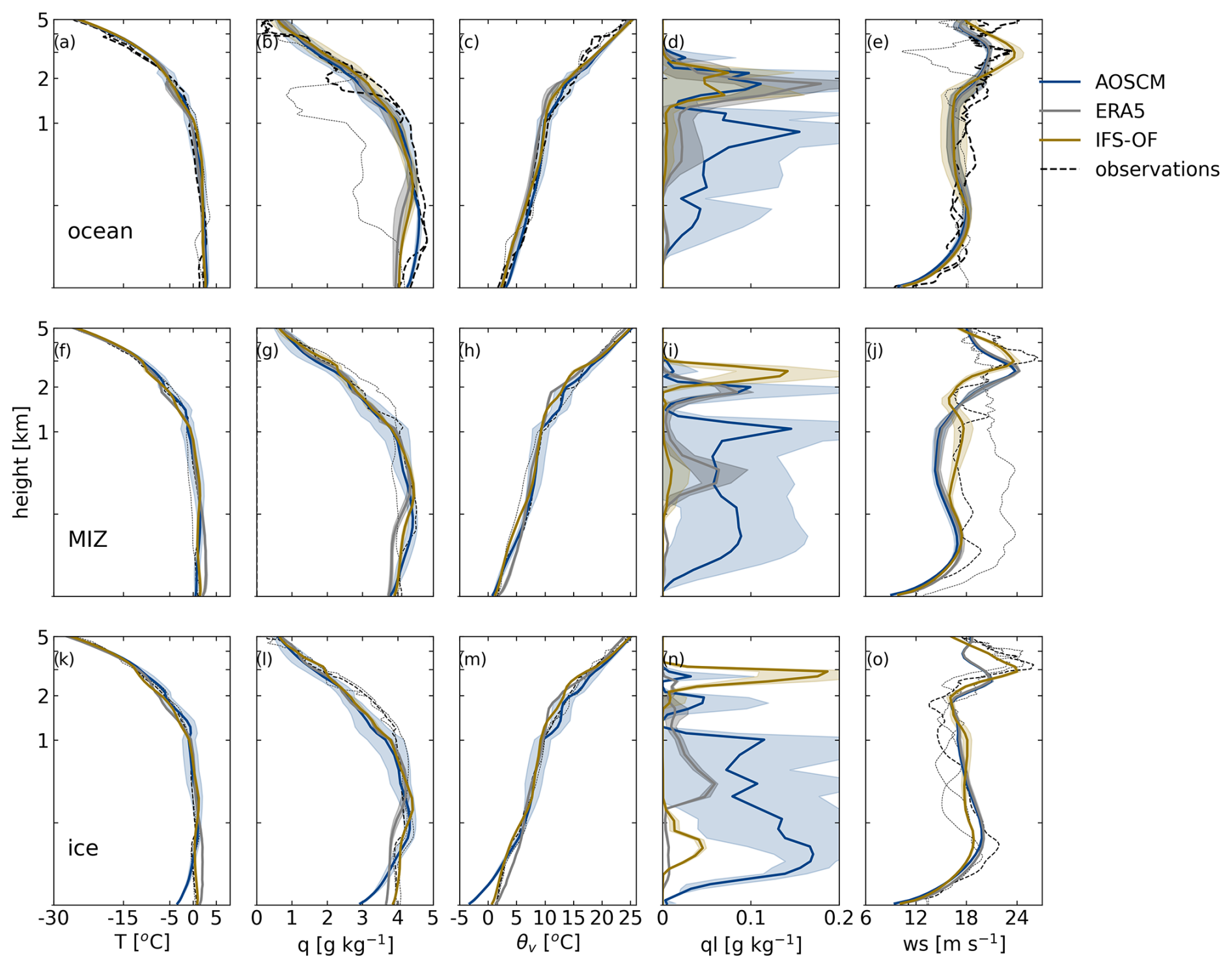
Figure 6 Vertical profiles of temperature (°C), specific humidity (g kg⁻¹), potential temperature, specific cloud liquid water content (g kg⁻¹), and wind speed (m s⁻¹) over the ocean (a–e), MIZ (f–j), and sea ice (k–o). Observations are shown with black dashed lines; their thickness represents their proximity to the AOSCM (blue), ERA5 (gray), and IFS-OF (gold) reference profiles for each surface type. The reference profiles were taken close to the majority of the observations (over or around the MIZ) and are denoted with black vertical lines in Fig. 5. The height axis is linear below 1 km and logarithmic above.

Variability in the observed specific humidity profiles is significant, especially over ocean (Fig. 6b). Two of the dropsondes match the AOSCM profile closely, while the third is considerably drier than all products. ERA5 and IFS-OF show a similar magnitude of specific humidity to the AOSCM except in the lowest 1 km where they both show a consistent deficit of approximately 0.3 g kg⁻¹. The air mass is observed to get progressively drier as it is advected over sea ice (Fig. 6g and l). Similarly to the cooling rate, the drying rate near the surface is overestimated by the AOSCM (Fig. 6l)

The air mass stratification remains strong over all surface types as demonstrated by the virtual potential temperature profiles, θ_v (Fig. 6c, h, and m). Near the surface, agreement with the AOSCM is strong, except over ice, where the simulated inversion appears much deeper, possibly due to the quick adjustment of the column to the more compact, colder sea ice surface.

The AOSCM specific liquid cloud content increases near the surface as the air mass is advected from the ocean (Fig. 6d) to the MIZ (Fig. 6i), indicating the formation of a secondary cloud layer that becomes even more prominent over fuller sea ice (Fig. 6n). Cloud profile measurements were not conducted during these research flights. However, the observed thermodynamic profiles over ocean and, more so, the MIZ and sea ice show small inversions within the first 2 km (Fig. 6c, h, and m). These inversions possibly correspond to a multilayer cloud structure that agrees with our AOSCM simulations, as well as ERA5 and IFS-OF (Fig. 6i–n).

The strong nudging in our AOSCM simulations makes the horizontal wind identical to ERA5 and, thus, comparable in magnitude and structure to observations (Fig. 6e, j, and o). The largest differences are noted, once again, in the lowest 2 km over the MIZ, where measurements capture a considerably stronger jet than the one in ERA5 and IFS-OF (Fig. 6j).

3.3.6 Physical and dynamical drivers

In order to reveal the physical mechanisms responsible for the different stages of the transformation we break down the changes in temperature and moisture (Fig. 7) within the air mass into the individual contributions of the participating physical parameterization schemes. These mechanisms impact different layers within the air mass: the planetary boundary layer (PBL), the liquid cloud layer, and the air aloft. We use the Ri_bulk-based diagnostic to isolate the PBL (see Sect. 3.3.4). The liquid cloud layer is identified as the layer between the PBL top and the liquid cloud layer top, therefore not including PBL clouds and ice clouds at altitudes higher than the liquid layer. Clouds exclusively in the ice phase are thus shown in the residual layer between the cloud layer top and 10 km. In Fig. 7 we show the ensemble mean physical tendency profiles contributed by each parameterization scheme, over the three different legs of the trajectories (ocean, MIZ, ice), for each of the three layers defined above (PBL, cloud, 10 km) separately, normalized by their individual depths.

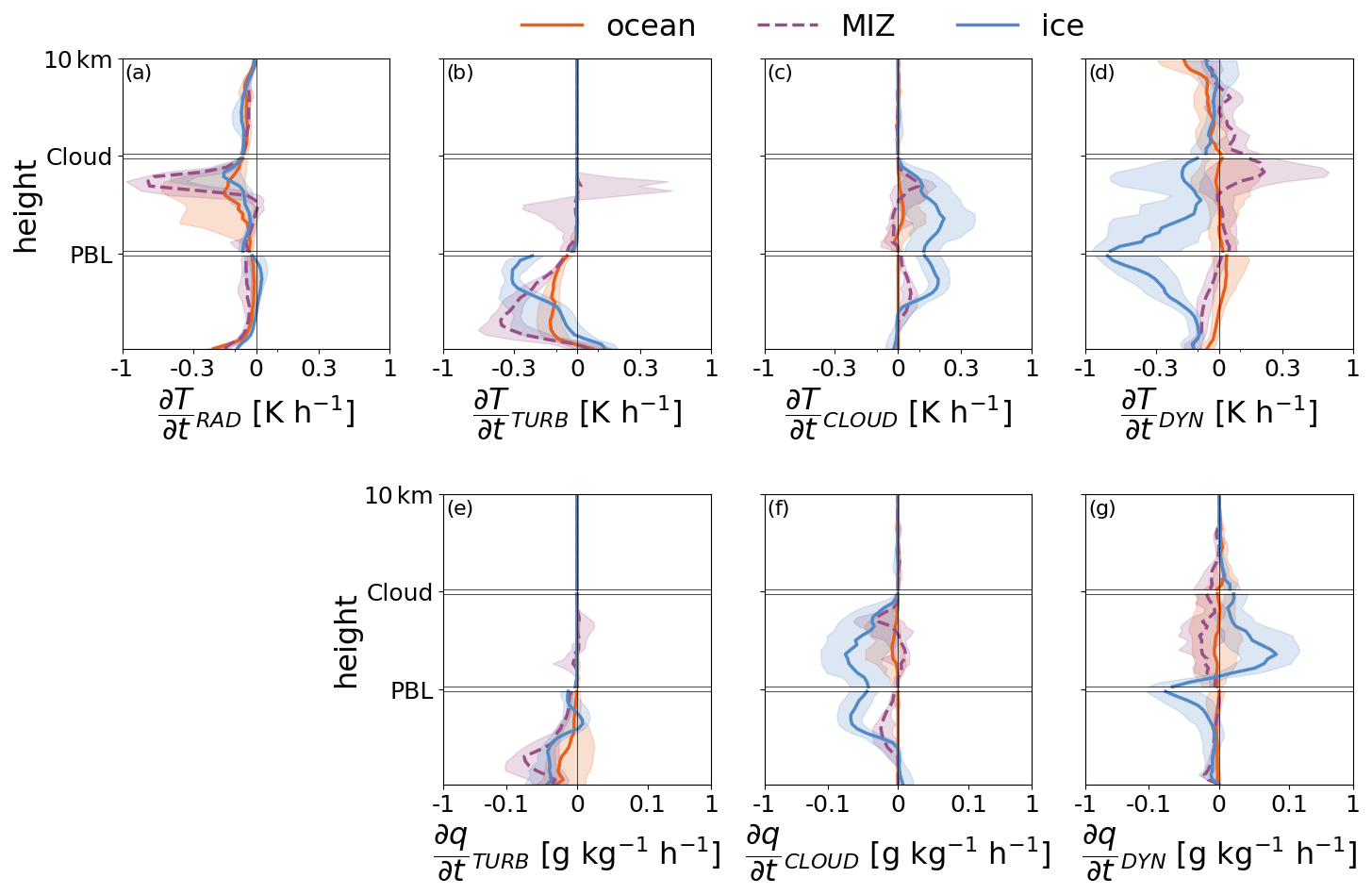
Figure 7 In the top row (a–d), tendencies of temperature (K h⁻¹) are presented attributed to (a) radiation (${\frac{\partial T}{\partial t}}_{\text{RAD}}$), (b) turbulence (${\frac{\partial T}{\partial t}}_{\text{TURB}}$), (c) cloud (${\frac{\partial T}{\partial t}}_{\text{CLOUD}}$), and (d) dynamical processes (${\frac{\partial T}{\partial t}}_{\text{DYN}}$) over the ocean (orange), MIZ (purple), and sea ice (blue) leg. The bottom row (e–g) is the same as the top but for changes of specific humidity ($\mathrm{g}{\mathrm{kg}}^{-\mathrm{1}}{\mathrm{h}}^{-\mathrm{1}}$). The ensemble median tendency profiles (solid lines) and the 25th and 75th percentiles (shaded areas around solid lines) have been computed over the length of their corresponding leg of the transformation, separately for three sublayers within the air mass (PBL, liquid cloud, and residual layer up to 10 km).

In the AOSCM, longwave radiative cooling is a prominent heat sink for the air mass throughout intrusion (Fig. 7a). Radiative cooling near the surface is largest over the ocean, approximately −0.2 K h⁻¹, where the near-surface air is warmest and most humid, and drops to −0.1 K h⁻¹ over the MIZ and sea ice. The ensemble median cooling rates derived from the radiation scheme also spike, as expected, at the top of the liquid cloud layer, reaching values of −0.15, −0.5, and −0.15 K h⁻¹ over the ocean, MIZ, and sea ice, respectively. The variability over ocean and sea ice in the radiative cooling rates within the cloud layer is the largest due to differences in cloud-top height and/or temperature in those sections of the air mass transformation. Over the MIZ, the cloud developing within the boundary layer causes an additional local radiative cooling of −0.05 K h⁻¹.

Turbulent processes are also efficient in removing heat and moisture from the air mass, but their effect is confined within the boundary layer (Fig. 7b and e). Over the ocean, the turbulent heat loss is weaker, around −0.15 K h⁻¹ in the middle of the PBL and gradually dropping to zero at the top. As the stratification becomes stronger, the turbulent cooling rates grow to −0.4 K h⁻¹ over the MIZ. While the turbulent cooling for the ocean and MIZ is more uniformly distributed within the PBL, over sea ice the temperature tendency drops almost linearly with height, reaching a minimum of −0.3 K h⁻¹ near the PBL top.

${\frac{\partial T}{\partial t}}_{\text{TURB}}$ turns weakly positive (around −0.05 K h⁻¹) near the surface for all legs. This could be in response to the near-surface cooling induced by radiation (Fig. 7a) and dynamics (Fig. 7d). Turbulence induced by radiative cooling at the cloud top mostly redistributes heat and moisture within the cloud layer, more prominently over the MIZ where cloud liquid water content and cloud-top radiative cooling are, on average, largest. Turbulent tendencies, as well as fluxes (not shown), of both heat and moisture drop to zero near cloud base. This is an indication that the cloud layer, as defined here, is generally decoupled from the surface and has no part in the overturning of the boundary layer and the consequent downward mixing of heat and moisture. With the exception of the time the air mass spends over the MIZ when new cloud formation occurs within the boundary layer, the rest of the time, turbulent fluxes near the surface are solely mechanically driven.

Turbulent processes appear to be consistently depleting the air mass of its moisture throughout the transformation (Fig. 7e), even over ocean. While it is possible for moisture deposition to temporarily occur over aquatic surfaces, we consider the magnitude and persistence of it in our AOSCM simulations and ERA5 (Fig. 3h) to be overestimated. A potential explanation for this overestimation could be the excessive downward mixing of heat and moisture by the IFS PBL scheme in stable conditions (Sandu et al., 2013; Holtslag et al., 2013).

The AOSCM cloud scheme drives changes in the air mass temperature and moisture through the release and consumption of latent heat during evaporation and condensation processes (Fig. 7c and f). During the oceanic leg of the air mass transformation, the cloud varies little, with weakly positive mean tendencies in the top part of the cloud layer due to some overall small cloud liquid water growth and negative tendencies towards the cloud base due to evaporation of precipitation. The liquid cloud grows over the MIZ, possibly due to the enhanced radiative cooling at the time, while a new cloud layer is formed in the boundary layer, where the condensation-related temperature tendencies, equal to 0.1 K h⁻¹, partially offset the radiative and turbulent cooling. In the residual layer, small peaks in ${\frac{\partial T}{\partial t}}_{\text{CLOUD}}$ show small changes in the overlying ice cloud. Over sea ice, the cloud scheme produces major warming, as high as 0.3 K h⁻¹, for both the boundary and the overlying liquid cloud layers.

The dynamic tendencies of temperature (${\frac{\partial T}{\partial t}}_{\text{DYN}}$, Fig. 7d) and moisture (${\frac{\partial q}{\partial t}}_{\text{DYN}}$, Fig. 7g) in the absence of horizontal advection as required in this Lagrangian single-column framework represent both vertical transport and the adiabatic temperature changes that come as a result of the prescribed subsidence conditions. Over the ocean, the adiabatic tendencies are mostly insignificant. The median profiles show minor warming (0.05 K h⁻¹) over the top half of the boundary layer, potentially corresponding to the consistent low-level large-scale subsidence pulse shown in Fig. 5p, while closer to the surface, ${\frac{\partial T}{\partial t}}_{\text{DYN}}$ turns slightly negative (−0.005 K h⁻¹). Over the MIZ, ${\frac{\partial T}{\partial t}}_{\text{DYN}}$ changes sign again, on average cooling the boundary layer by 0.1 K h⁻¹ while weakly warming the cloud layer by 0.05 K h⁻¹. However, the 75th percentile reaches up to 0.5 K h⁻¹ at the top of the cloud layer. In the MIZ, the cloud takes up a larger part of the 5 km layer, making the effect of the adiabatic warming more significant and explaining the change of slope in the ${\stackrel{\mathrm{‾}}{T}}_{\mathrm{5}\mathrm{km}}\sim {\text{IWV}}_{\mathrm{5}\mathrm{km}}$ diagram (Fig. 4). The strong upward motion over the sea ice leg (Fig. 5p) results in a strong adiabatic cooling throughout the air mass, with the inversions at the top of the boundary and liquid cloud layer once again being the most sensitive to the temperature changes induced by the vertical motion. Adiabatic cooling appears to be responsible for the accelerated loss of heat within the air mass over sea ice, as well as moisture, considering the mirroring appearances of ${\frac{\partial T}{\partial t}}_{\text{DYN}}$ and ${\frac{\partial T}{\partial t}}_{\text{CLOUD}}$, with the latter showing rapid condensation in response to large-scale updrafts (Fig. 7g) that depletes of the moisture content of the air mass.

It should be noted that, at the end of the simulation period, the air mass has an IWV_5 km of 8 kg m⁻² (Fig. 4), which makes it still anomalously moist (and subsequently warm) compared to the 1979–2019 climatological median of approximately 2 kg m⁻² (Rinke et al., 2021). The air mass transformation is, therefore, not complete and could go on for several days as is typical for WAIs in the Atlantic sector (Woods and Caballero, 2016). In this specific case, the second warm-air intrusion that is set up to take place the next day (15 March) will likely mix with the leftover moisture from the previous episode and cease the transformation process prematurely. But large-scale dynamics are important for the future of the remaining heat and moisture even before the merge. The large-scale updraft that dominated the transformation over sea ice resulted in a temperature decrease of 6 °C, triple in magnitude compared to that exerted by radiation and turbulent mixing combined (Fig. C1). If the air mass continued to be lifted and, thus, lose heat and moisture at the same rate, IWV could drop to typical Arctic air mass values in the next 24 h. In milder subsidence conditions, temperature changes would be driven mostly by radiative cooling (Fig. C1). The emitted longwave radiation, however, would grow weaker as the temperature dropped and the liquid clouds dissipated, requiring more time for the transformation to reach completion.

The role of subsidence has not been adequately accounted for in the mostly idealized WAI air mass transformation modeling studies that have been attempted to date (Pithan et al., 2018). Part of the reason lies in the lack of observations and/or observational methods for the large-scale vertical motion, making reanalysis products, such as ERA5, the most common source for forcing information in SCM and LES experiments. The HALO-(𝒜𝒞)³ campaign (Wendisch et al., 2024) attempted to measure the large-scale subsidence on multiple counts (Paulus et al., 2024), including a cold-air outbreak event. Their results showed variable agreement between measurements and ERA5 reanalysis, at times displaying a significant mismatch in the magnitude and even sign of vertical velocity (ω). In this context, it is difficult to determine whether the prescribed subsidence profiles in our simulations and their consequent impact on the air mass transformation are realistic.

4 Conclusions

We studied the air mass transformation of a mid-March warm-air intrusion (WAI) using Lagrangian single-column simulations and observations collected by the HALO-(𝒜𝒞)³ aircraft campaign. Our trajectory analysis of the WAI event is in agreement with the findings of Svensson et al. (2023); air parcels transported at different heights within a 5 km deep column align vertically. Through further investigation using ERA5 reanalysis data, we conclude that the aligned trajectories are representative of the advected air mass to a satisfactory degree. The air mass ability to maintain a column-like structure throughout the WAI event motivated us to construct and apply a Lagrangian single-column modeling framework based on the Atmosphere–Ocean Single-Column Model (AOSCM, Hartung et al., 2018).

In our framework, advection is represented through the temporal changes in the surface and dynamical forcing. In addition, we use the aligned trajectories to perform ensemble simulations of the air mass transformation, thus incorporating the variability of the air mass properties as well as the different forcing scenarios the air mass realistically may be subjected to along its track. Comparing to observations, ERA5 reanalysis, and IFS operational forecast data (IFS-OF), we found that the model adequately reproduces the magnitude and timescales of the transformation, from the bulk changes in heat and moisture content to the evolution of the vertical thermodynamic and cloud structure. During the advection over ocean and in the absence of strong large-scale subsidence conditions, radiation and boundary layer processes deplete the air mass heat content, while over the MIZ, the moisture condenses into a multilayer cloud. Deeper into the Arctic, large updrafts accelerated the heat loss through adiabatic cooling and consequently enhanced the drying response of cloud and precipitation processes.

The AOSCM struggled to represent the evolution of the stable boundary layer throughout the simulation. The demonstrated biases were, in part, expected due to the overly diffusive closure in stable conditions implemented in IFS (Sandu et al., 2013; Holtslag et al., 2013). Furthermore, errors in our simulations may have arisen from the large dependence on the along-track prescribed ERA5 vertical velocity, the accuracy of which is inconsistent (Paulus et al., 2024). It is important to note that the large-scale updrafts applied in our simulations would normally be accompanied by low-level convergence and, therefore, advection of new air in the column, which is prohibited in our framework. Another issue could be our Lagrangian framework's simplifications, such as the exclusion of trajectories within the boundary layer and the abrupt transitions between the different surface regimes.

In conclusion, our Lagrangian AOSCM framework is a novel tool that facilitates the simulation of realistic WAI events and, therefore, the direct evaluation with observations and can virtually be applied to simulate any case of meridional air mass transport. The AOSCM shares the same physical parameterizations as EC-Earth and OpenIFS, and, despite being conceptually simpler and significantly less resource-intensive, it is able to reconstruct an air mass transformation similar to its global counterpart. This makes the model well-suited for wider application to more warm-air intrusion and cold-air outbreak events that have been captured over time by ship and aircraft campaigns. A more expansive study using the Lagrangian AOSCM framework would be valuable for identifying common features among air mass transformations. The model's ability to separate physical processes from the complex dynamics of WAIs can help uncover persistent Arctic-related model biases, mitigate long-standing parameterization deficiencies, and eventually improve weather forecasts and climate projections.

Appendix A: Cloud radiative forcing

Figure A1 Same as Fig. 3 but for (a) shortwave and (b) longwave cloud radiative forcing at the surface and (c) surface albedo.

Appendix B: Surface energy budget in the AOSCM

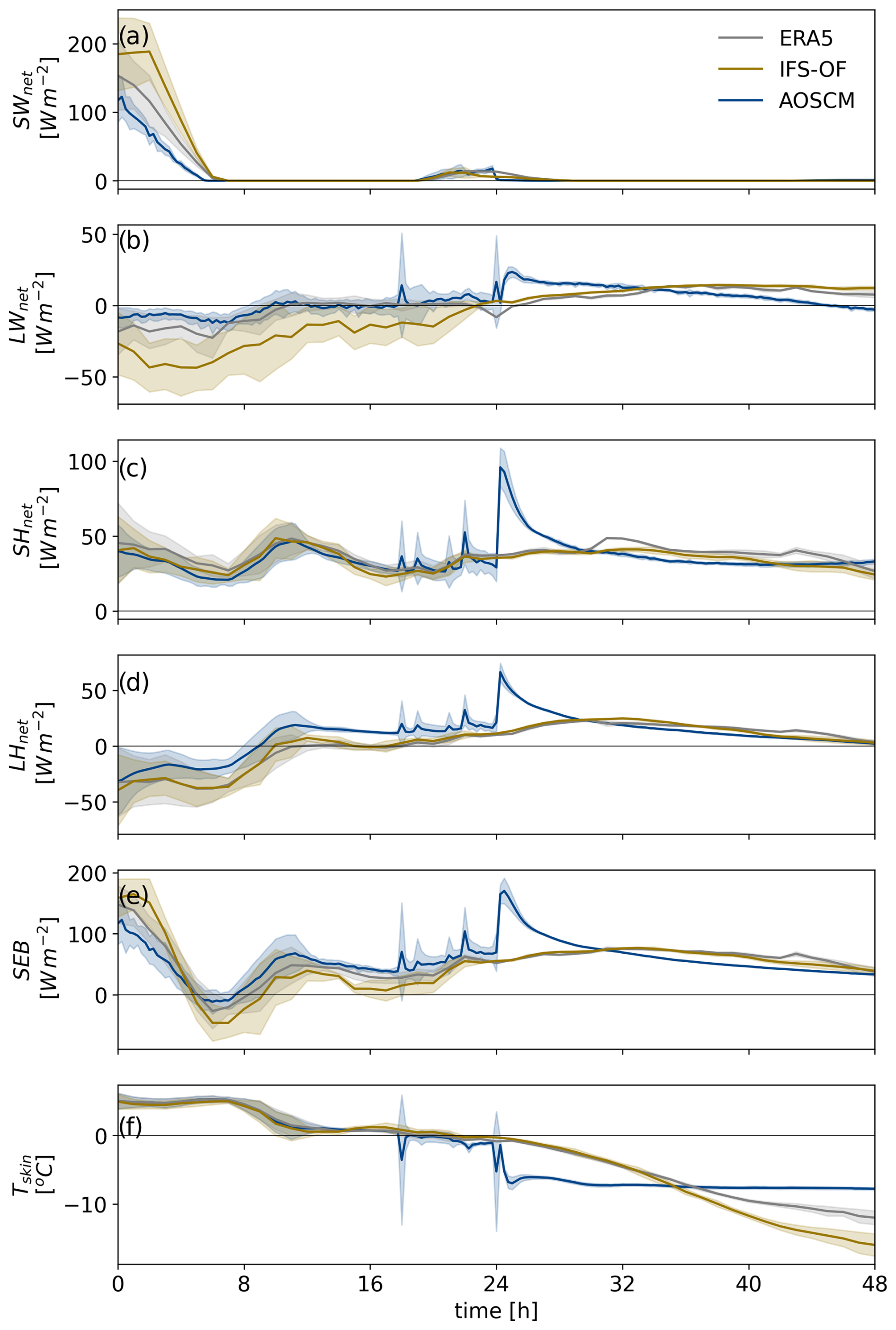
Figure B1 Time series of the surface (a) shortwave radiative, (b) longwave radiative, (c) sensible heat, and (d) latent heat fluxes, as well as (e) the surface energy budget and (f) the skin temperature along the trajectories. The AOSCM, ERA5, and IFS-OF are drawn with blue, gray, and sand, respectively.

Appendix C: Time-integrated cooling contributions

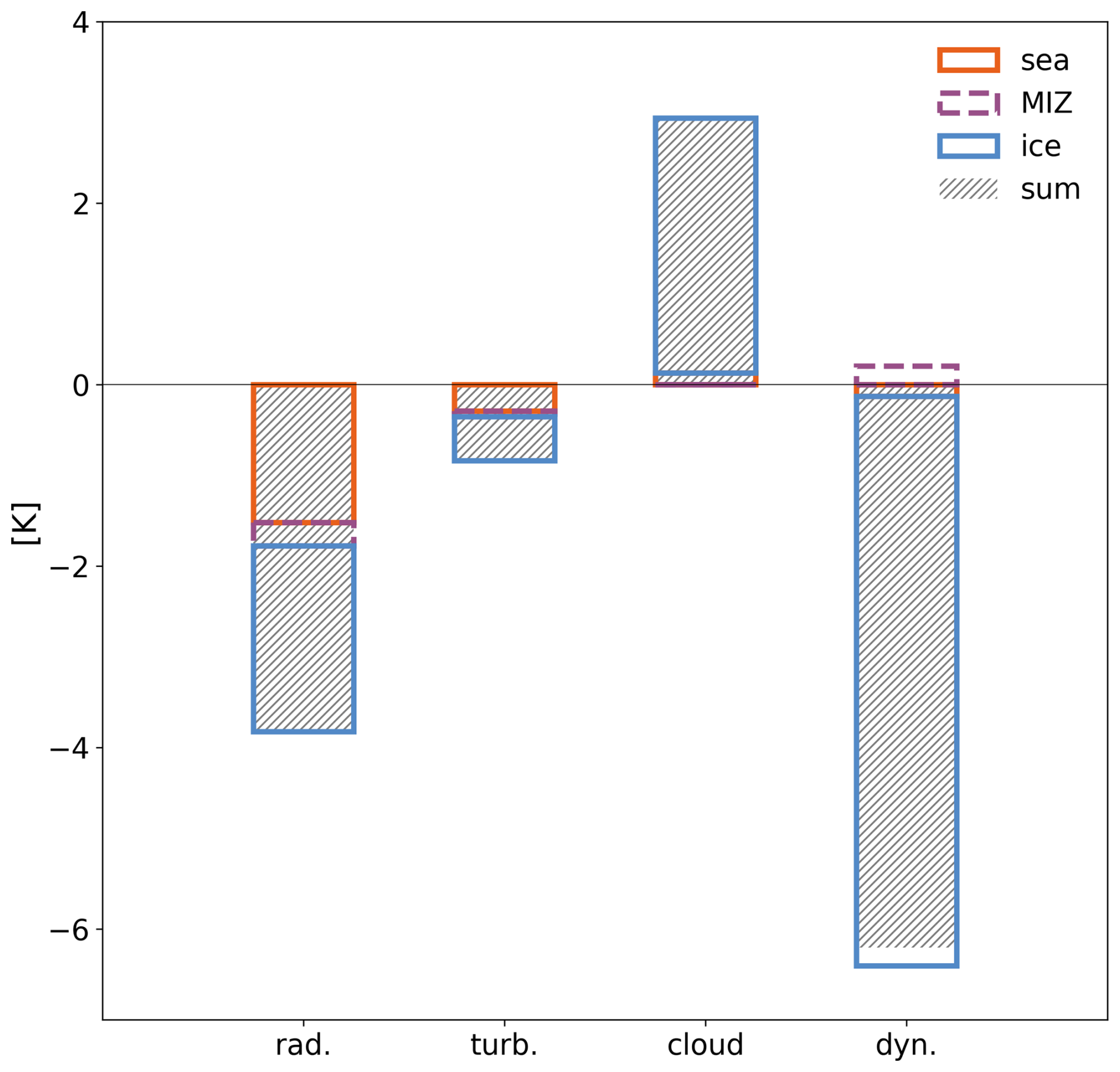
Figure C1 Time-integrated temperature changes contributed by radiation, turbulence, cloud processes, and adiabatic cooling. Different colors are used to show the changes per transformation leg (ocean, MIZ, ice) and hatches to show the sum over the entire transformation.