Comparing multi-model ensemble simulations with observations and decadal projections of upper atmospheric variations following the Hunga eruption

The Hunga Tonga–Hunga Ha'apai Model–Observation Comparison (HTHH–MOC) project aims to comprehensively investigate the evolution of volcanic water vapor and sulfur emissions and their subsequent atmospheric impacts and underlying response mechanisms using state-of-the-art global climate models. This study evaluates multi-model ensemble simulations participating in the HTHH–MOC free-run experiment with climate projections for 10 years (2022–2032). Model results are evaluated against satellite observations to assess their ability to reproduce the observed evolution of stratospheric water vapor, aerosols, temperature, and ozone from 2022 to 2024. The participating models accurately capture the observed distribution patterns and associated upper atmospheric responses, providing confidence for their future projections. Model simulations suggest that the Hunga eruption-induced stratospheric water vapor anomaly lasts 4–7 years, with a water vapor e-folding time of 31–43 months. This prolonged water vapor perturbation leads to significant stratospheric and mesospheric cooling, resulting in significant ozone loss in the upper stratosphere and lower mesosphere for 7–10 years. Comparisons between simulations with both SO₂ and H₂O emissions and those with H₂O-only emissions indicate that the pronounced dipole response with upper-stratospheric cooling and lower-stratospheric warming is driven by the combined effects of SO₂ and H₂O injections. These results highlight the prolonged atmospheric impacts of the Hunga eruption and the potential critical role of stratospheric water vapor in modulating long-term atmospheric chemistry and dynamics.

1 Introduction

Explosive volcanic eruptions typically inject substantial amounts of sulfur dioxide (SO₂) into the stratosphere, where it converts to sulfate aerosols that reflecting incoming shortwave radiation while absorbing longwave radiation, resulting in surface cooling and stratospheric warming (Robock, 2000; Timmreck, 2012). However, the January 2022 Hunga Tonga–Hunga Ha'apai (HTHH) eruption (hereafter referred to as Hunga; Carr et al., 2022) challenged this conventional understanding. While the Hunga eruption injected only a moderate amount of SO₂, an exceptionally large quantity of water vapor (H₂O) remained in the stratosphere and mesosphere, with initial injections reaching altitudes as high as 55 km (Carr et al., 2022).

Based on in-situ measurements and satellite data retrievals, the Hunga eruption injected approximately 0.4–0.5 Tg of SO₂, with an injection altitude of 25–40 km (Millán et al., 2022; Carn et al., 2022). However, Sellitto et al. (2024) suggested a potentially higher SO₂ mass exceeding 1.0 Tg. Unlike previous explosive eruptions, Hunga injected an estimated ∼ 150 Tg of H₂O into the stratosphere and mesosphere, with concentrations peaking at 25–30 km (Millán et al., 2022). Ground-based millimeter-wave spectrometer observations detected an anomalous transport of water vapor up to 70 km during the winter of 2023 (Nedoluha et al., 2024). This substantial water vapor injection leads to stratospheric cooling of 0.5–1 K from early 2022 to mid-2023, followed by mesospheric cooling of 1.0–2.0 K, as observed in satellite data (Wang et al., 2023; Stocker et al., 2024; Randel et al., 2024). The cooling was primarily driven by the radiative effects of H₂O in the stratosphere, while ozone (O₃) loss played a key role in mesospheric cooling (Randel et al., 2024).

The enhancement of stratospheric H₂O during the first three months following the Hunga eruption was well reproduced in 10-month simulations using three ensemble members of the coupled CESM2–WACCM–CARMA (Zhu et al., 2022). Niemeier et al. (2023) conducted two-year-long, single-member simulations with the ICON–Seamless model to investigate water vapor transport under different Quasi-Biennial Oscillation (QBO) phases, finding that the simulated transport patterns closely aligned with Microwave Limb Sounder (MLS) observations. The evolution of H₂O was also well reproduced by Zhou et al. (2024) using an offline 3-D chemical transport model (CTM). Using the two-dimensional GSFC2D model, Fleming et al. (2024) performed a 10-year simulation, which indicated approximately 1 K warming in the lower stratosphere, 3 K cooling in the mid-stratosphere, and a variable ozone response across different pressure levels and polar regions. Wang et al. (2023) and Randel et al. (2024) performed ensemble simulations with 10 members using CESM2–WACCM6, incorporating both H₂O and SO₂ injections. Their simulations successfully captured the observed temperature and ozone changes in the stratosphere and above, focusing on the first several years of the simulation. These single-model studies, which primarily considered only water vapor injection with limited realizations or short simulation durations (Zhu et al., 2022; Niemeier et al., 2023; Zhou et al., 2024), provide a limited understanding of the full evolution of the Hunga eruption. Although Fleming et al. (2024) explored decadal-scale impacts, they considered the H₂O injection only and did not include aerosol–chemistry interactions. Therefore, comparisons of multi-model simulations with larger ensemble sizes and longer time horizons are needed to fully understand both the short-term (months to two years) and long-term (multi-year to decadal) evolution of Hunga volcanic emissions and their atmospheric impacts.

In mid-2023, the research community initiated an Hunga Impact Activity within the World Climate Research Programme (WCRP) Atmosphere Processes And their Role in Climate (APARC). This ongoing three-year project aims to integrate modeling and observational efforts to systematically evaluate Hunga volcano impact model observation comparisons (Zhu et al., 2025). A key objective is to understand the long-term evolution of the volcanic injections and to project the long-term impacts of the eruption using a multi-ensemble modeling approach. The reliability of these predictions critically depends on the performance of model simulations. This study aims at evaluating multi-model simulations against observations for the first two post-eruption years and projects variations up to a decade after the eruption, with a particular focus on the evolution of volcanic sulfur and water vapor injections and associated temperature and ozone changes in the stratosphere and lower mesosphere. Schoeberl et al. (2024) demonstrated that these four factors are the key variables that impact the radiative forcing from this eruption.

Following this introduction, Sect. 2 describes the methods, including the observational datasets and model simulations used in this study. Section 3 presents the results and discussion, focusing on comparisons of selected variables and their long-term variations. The analysis is structured in the following order: stratospheric aerosol optical depth (SAOD), water vapor (SWV), temperature, and ozone variations in the stratosphere and lower mesosphere. Finally, Sect. 4 provides a summary and conclusions.

2 Methods

2.1 Satellite observational data

Water vapor (H₂O), temperature and ozone (O₃) data were obtained from version 5 (v5) retrievals of the Microwave Limb Sounder (MLS) satellite observations (Livesey et al., 2020; Waters et al., 2006). The MLS instrument, launched aboard the Aura satellite in 2004, operates in a sun-synchronous, near-polar orbit. It measures a range of atmospheric properties and constituents across five broad microwave spectral regions, with central frequencies at 118, 190, 240, 640 and 2500 GHz.

The vertical resolution of MLS H₂O data ranges from approximately 1.3–3.6 km between 316–0.22 hPa and 6–11 km between 0.22–0.1 hPa. The MLS H₂O data are deseasonalized relative to the 2012–2021 pre-eruption climatology, and Hunga anomalies are calculated with respect to pre-eruption values. Since MLS observations have been limited to several days per month starting in April 2024, monthly averages are calculated based only on the available observation days from April to November 2024 to extend the record of stratospheric water vapor (SWV) mass evolution for as long as possible. The vertical resolution of temperature measurements is approximately 3–4 km for 100–10 hPa and 5–6 km for 10–0.1 hPa. O₃ retrievals have a vertical resolution of approximately 3 km for 100–1 hPa and 5 km for 1–0.1 hPa. To enable a more direct comparison between model simulations and observations, the MLS temperature and ozone data have been detrended to eliminate the long-term temperature trend and adjusted to remove variability associated with the 11-year solar cycle, ENSO, and QBO using regression analysis (Randel et al., 2024).

Stratospheric aerosol optical depth (SAOD) data from the Global Space-based Stratospheric Aerosol Climatology (GloSSAC; Thomason et al., 2018; Kovilakam et al., 2020, 2023) is used as observational data. Aerosol extinction and surface area density (SAD) data from both GloSSAC and version 2.1 of the Ozone Monitor and Profiler Suite Limb Profiler (OMPS; Taha et al., 2021, 2022) are incorporated into the GSFC2D model simulations. The OMPS-derived SAOD is calculated from the model input of OMPS aerosol extinction data.

2.2 Model experiments following the HTHH–MOC protocol

Model simulations are essential for projecting the long-term evolution of volcanic injections and understanding their subsequent atmospheric and climate impacts and mechanisms behind the observed phenomena. The HTHH–MOC project protocol designed two groups of experiments, with the first experiment (Exp1) requiring a 10-year simulation. These decade-long simulations aim to investigate the long-term evolution of volcanic emissions and their impacts on ozone chemistry, radiation, and surface climate (Zhu et al., 2025).

Five models participated in Exp1 including four three-dimensional general circulation models (GCMs): the Community Earth System Model version 2 (CESM2) (Gettelman et al., 2019), with the Whole Atmosphere Community Climate Model version 6 (WACCM6) (Mills et al., 2016) as its atmospheric component and four-mode modal aerosol module (MAM4; Liu et al., 2012, 2016; Mills et al., 2016) as its aerosol module (WACCM6MAM in this study), the NASA Goddard Earth Observing System Chemistry–Climate Model (GEOSCCM) (Nielsen et al., 2017), the Model for Interdisciplinary Research On Climate version 6 – Chemical Atmospheric General Circulation Model for Study of Atmospheric Environment and Radiative Forcing (MIROC–CHASER) with three-mode modal aerosol module (Sekiya et al., 2016), and the Canadian Middle Atmosphere Model (CMAM) (Jonsson et al., 2004). In addition, the NASA/Goddard Space Flight Center two-dimensional chemistry–climate model (GSFC2D) (Fleming et al., 2024) participated in the simulations.

Each model was requested to conduct ensemble simulations with a default injection of 0.5 Tg SO₂. Due to differences in model configurations and available resources, the details of simulations and the number of ensemble members varied across models. The protocol did not prescribe a consistent injection mass of 150 Tg H₂O because models implement injection in different ways, and ice clouds can rapidly form and remove H₂O after the initial injection. Instead, models were instructed to retain approximately 150 Tg of water after the first couple of days of injection. The detailed initial water injection mass and the modeled maximum burden for each model are summarized in Table 1 and discussed in Sect. 3.2 of the results.

Mills et al. (2016)Mills et al. (2016)Nielsen et al. (2017)Sekiya et al. (2016)Sekiya et al. (2016)Jonsson et al. (2004)Scinocca et al. (2008)Fleming et al. (2024)Fleming et al. (2024)Fleming et al. (2024)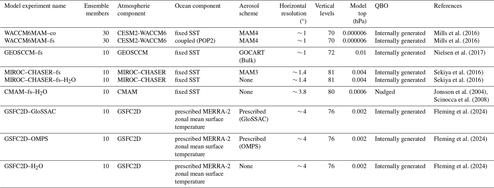

Table 1 Model experiment name and model information.

WACCM6MAM conducted simulations with both coupled ocean and fixed sea surface temperature (SST) configurations, labelled WACCM6MAM–co and WACCM6MAM–fs, respectively, while MIROC–CHASER–fs and GEOSCCM–fs used fixed SST only. The GSFC2D model prescribed aerosol injection using satellite–derived aerosol extinction data, with simulations labelled GSFC2D–GloSSAC and GSFC2D–OMPS based on the data used.

To isolate the effects of volcanic aerosols from those of H₂O, additional H₂O–only injection simulations were conducted. Three models (MIROC–CHASER–fs–H₂O, GSFC2D–H₂O, and CMAM–fs–H₂O), performed these simulations.

All five models also ran control simulations without volcanic injections. Model ensemble means were used in the analysis, and anomalies were computed by comparing the experimental simulations to the corresponding control runs. Statistical significance was assessed using a Student's t-test at the 95 % confidence level.

A summary of the experiment names, simulation details, and model configurations is provided in Table 1. Further details regarding the participating models and experiment protocols can be found in Zhu et al. (2025).

3 Results and discussions

3.1 Stratospheric aerosol optical depth (SAOD) anomaly

GloSSAC data indicate that the volcanic aerosols are predominantly concentrated in the Southern Hemisphere (SH), with a smaller fraction transported to the Northern Hemisphere (NH) tropics (Fig. 1). In the first few months of 2022, the aerosols remain largely trapped in the low latitudes of the tropical pipe (Taha et al., 2022). The SH (0–30° S) experiences a higher aerosol concentration compared to the NH tropics (0–30° N). From mid-2022, during the austral winter, more aerosols are transported to the SH mid-latitudes (30–60° S). The strong polar vortex in the austral winter and spring prevents further poleward transport (Manney et al., 2023). However, at the end of 2022 and the beginning of 2023, the break-up of the polar vortex during austral late spring–early summer allows for a slight poleward movement of aerosols toward the southern polar regions, with a minor portion also being transported northward toward the tropics. Following this, the aerosols are predominantly confined and transported in the SH mid-latitudes. This pattern reflects the influence of seasonal changes in the polar vortex and the Brewer-Dobson circulation on stratospheric aerosol transport (Butchart, 2014). OMPS observations show a similar latitudinal transport pattern over time, although exhibit stronger SAOD values in the tropics and southern mid-latitudes compared to GloSSAC.

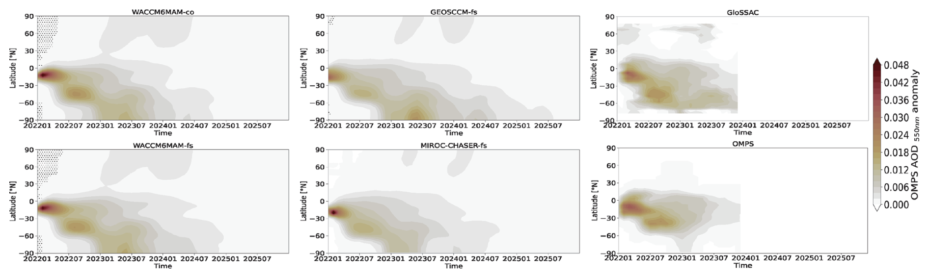
Figure 1 Hovmöller diagrams of global mean stratospheric aerosol optical depth (SAOD) anomalies following the Hunga eruption. The four left panels present ensemble mean anomalies from different models relative to the control run, with dotted areas indicating statistically insignificant anomalies at the 95 % confidence level based on Student's t-tests. The top-right panel shows the observed anomaly from the Global Space-based Stratospheric Aerosol Climatology (GloSSAC), relative to the 2012–2021 climatological period. The aerosol extinction of the GloSSAC data was used in the GSFC2D model as their prescribed aerosol field input (Zhu et al., 2025). The bottom-right panel displays the Stratospheric Aerosol Optical Depth (SAOD) calculated from aerosol extinction data obtained from the Ozone Monitoring and Profiler Suite Limb Profiler (OMPS), which was utilized in the GSFC2D model.

Model simulations demonstrate reasonable agreement with observed latitudinal SAOD distribution patterns (Fig. 1). Both GloSSAC and OMPS show a decrease in SAOD over time as aerosols are transported toward the SH high latitudes. WACCM6MAM–co, WACCM6MAM–fs, and MIROC–CHASER–fs all exhibit similar trends, although with a stronger SAOD in the tropics compared to the observations. In contrast, GEOSCCM–fs displays weaker SAOD in the tropics and a stronger SAOD in the polar regions (60–90° S) by mid-2023, compared to mid-latitudes (30–60° S) in mid-2022. Additionally, GEOSCCM–fs shows a larger SAOD anomaly in the SH polar latitudes during the boreal summers of 2024 and 2025, indicating that the SAOD anomaly may persist for a longer duration compared to other models, where the anomaly diminishes mostly by the end of 2024. These differences may stem from uncertainties on both the modeling and satellite observation sides, including variations in simulated aerosol microphysics and dynamics, as well as uncertainties in aerosol estimates from GloSSAC and OMPS retrievals. Understanding these differences and uncertainties is a key objective of the Tonga Model Intercomparison Project (Tonga–MIP; Clyne, 2024), which, as a parallel initiative, will also contribute to the Hunga Assessment Report (Zhu et al., 2025).

Both observational data and model simulations show that the SAOD anomaly induced by the Hunga eruption lasts for approximately two years in the SH low latitudes. Additionally, both sources are consistent in identifying a secondary peak in SAOD over SH mid-latitudes during the second austral winter in 2023. Model projections further suggest minor extensions of the SAOD anomaly into the third and fourth years in SH high latitudes, with the third-year signal being particularly robust across climate models and also independent of ocean-atmosphere coupling.

3.2 Water vapor variation

3.2.1 Global stratospheric water vapor (SWV) mass anomaly

The Hunga eruption leads to an unprecedented increase in stratospheric water vapor (SWV), significantly influencing global SWV loading. After removing background water vapor, the MLS observed SWV mass anomaly from the Hunga eruption initially stabilizes at approximately 135 Tg before beginning to decline in the spring of 2023 (Fig. 2). Following a slight increase in late 2023, it starts decreasing more rapidly in early 2024, reaching ∼ 70 Tg by the end of 2024. The initial SWV mass analyzed based on the v5 retrieval of MLS is slightly lower than previous estimates, which, using the v4 retrieval of MLS indicated a ∼ 150 Tg water vapor injection by the Hunga eruption (Carr et al., 2022; Millán et al., 2022).

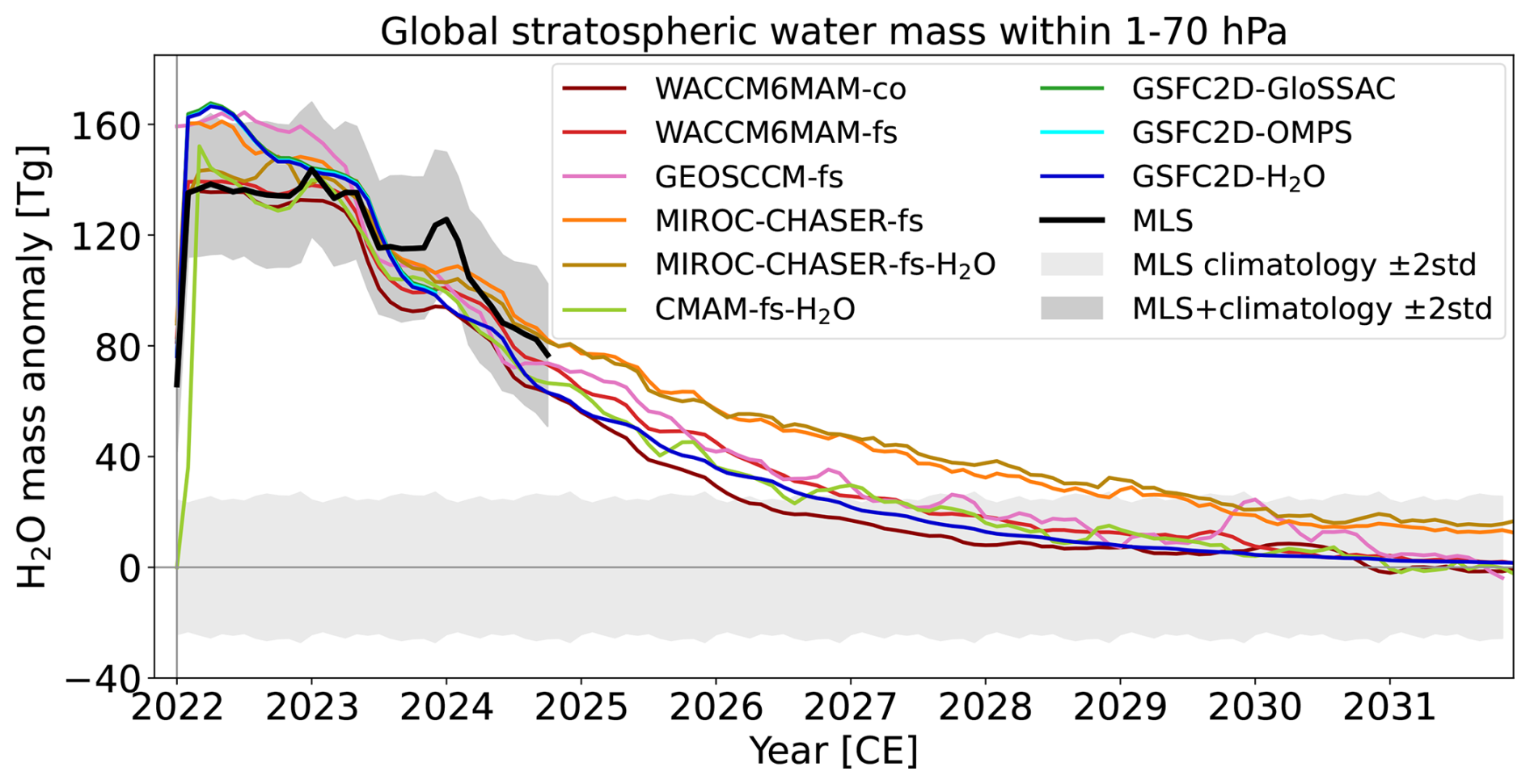
Figure 2 Simulated and observed global stratospheric H₂O mass anomalies within the 1–70 hPa range following the Hunga eruption. The colored lines represent the ensemble mean anomalies relative to the control run, while the black line and gray shading depict the observed anomaly from the Microwave Limb Sounder (MLS) water vapor mass, along with its ±2 standard deviation range from the 2012–2021 climatology period. GSFC2D–GloSSAC and GSFC2D–OMPS have only 2 years of simulations and are superseded by GSFC2D–H₂O with 10 years of simulations.

Compared to MLS observations, the modeled SWV mass anomalies exhibit varying evolutionary trends. WACCM6MAM–co and WACCM6MAM–fs replicate the MLS observations well, with an initial mass of approximately 135–140 Tg and a continuous plateau in SWV mass before it begins decreasing in early 2023. Despite an initial injection mass of 150 Tg, the rapid reduction of 10–15 Tg is attributed to the water vapor saturation effect, which converts water vapor into ice clouds during the first week after injection, as described by Zhu et al. (2022). GEOSCCM–fs also shows a similar initial plateau but with a larger magnitude of SWV mass compared to MLS in early 2022. A more pronounced decrease begins at the end of 2022, with the SWV mass eventually decreasing to a level comparable to MLS by early 2023. MIROC–CHASER–fs exhibits a larger initial water mass but with a shorter plateau, beginning its decrease by mid-2022. It also decreases to a comparable mass to MLS in early 2023. In contrast, MIROC–CHASER–fs–H₂O shows a similar initial mass and plateau to MLS, but with a slightly faster decrease at the end of 2023 compared to both MLS and MIROC–CHASER–fs. CMAM–fs–H₂O shows a slightly larger initial SWV mass but displays a similar variation in 2023 and a comparable decreasing trend thereafter. Simulations from GSFC2D–GloSSAC, GSFC2D–OMPS, and GSFC2D–H₂O exhibit nearly identical SWV mass evolution, characterized by a shorter plateau and a more significant decline starting in mid-2022.

Background variability in the MLS observational record is calculated using 2–sigma interannual deviations over the 2005–2021 pre-Hunga period. When considering the variation in MLS observations, all modeled SWV mass anomalies fall within the two standard deviation range of the MLS data, indicating that the model simulations reasonably reproduce the observed evolution patterns. Additionally, the modeled SWV mass decreasing slope in late 2023 is not as sharp as in early 2023, with a slight increase observed at the end of 2023 or early 2024 in models such as WACCM6MAM–co, GEOSCCM–fs, and MIROC–CHASER–fs, although this increase is less pronounced compared to the one observed in MLS at the end of 2023.

Millán et al. (2024) estimated that the anomalous state induced by the Hunga eruption could diminish within 5–7 years based on an exponential decay using MLS observations – a timescale that closely aligns with projections from the model simulations in this study. Among the simulations, the only one with a coupled ocean (WACCM6MAM–co) exhibits the shortest perturbation duration, with stratospheric H₂O mass returning to climatological levels within four years (by 2026). This may reflect a faster transport and more efficient H₂O removal process in the coupled ocean simulation compared to the fixed-SST configuration. Additional model simulations with coupled oceans are needed to confirm this. The longest perturbation, lasting up to seven years (until 2029), is projected by MIROC–CHASER–fs, while the other models suggest a duration of approximately 5 years, until 2027. The current decreasing trend in MLS H₂O mass lies within the range of model projections, suggesting a potential perturbation lasting around five years. This prolonged anomaly has significant implications for the climate system.

Table 2 Initial injection and e-folding time of water mass in different model simulations.

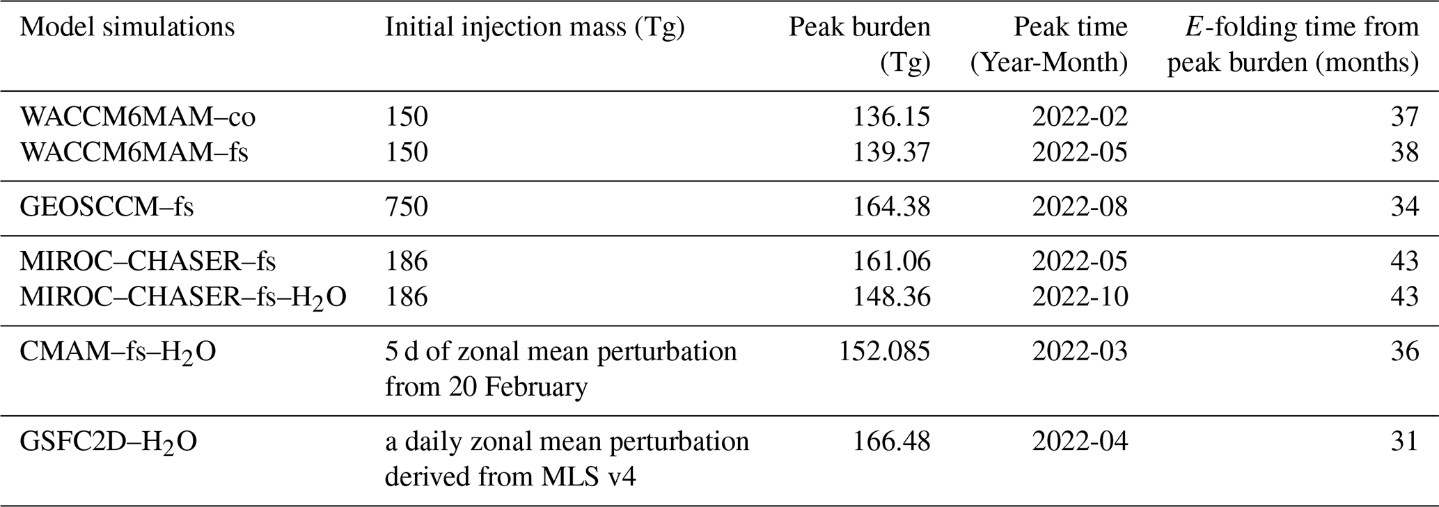
The e-folding time of stratospheric H₂O mass is typically calculated from the initial injection; however, the HTHH–MOC protocol mandates a retained H₂O mass of ∼ 150 Tg in January 2022. Due to variations in how models simulate the initial ice cloud formation and removal processes, the initial H₂O injection methods and magnitudes differ across models, as summarized in the second column of Table 2. The lowest initial injection occurs in WACCM6MAM–co and WACCM6MAM–fs at 150 Tg, whereas GEOSCCM–fs injects the highest amount at 750 Tg. Given this wide disparity, calculating e-folding time from the initial injection would be inappropriate. Instead, we use the e-folding time from the peak H₂O mass as a more consistent metric for assessing H₂O lifetime.

The maximum H₂O mass across models generally falls within the range of 130–160 Tg. Prior to initiating the ensemble simulations, model adjustments were made to achieve the protocol target of retaining 150 Tg of H₂O by the end of January 2022. However, due to internal variability within free-running models, individual ensemble members exhibit different evolutionary trajectories, leading to variations in maximum H₂O burden among members (Fig. A1). Additionally, differences in microphysical and dynamical processes across models further contribute to variations in both the peak H₂O mass and the timing of peak occurrence. WACCM6MAM–co reaches its peak of 136 Tg the fastest, within two months, whereas MIROC–CHASER–fs–H₂O takes the longest, requiring ten months to reach 148 Tg. The earliest e-folding time from peak mass occurs in November 2024 in GSFC2D–H₂O, while MIROC–CHASER–fs-H₂O exhibits the latest, in May 2026, with corresponding e-folding times of 31 and 43 months, respectively.

Interestingly, MIROC–CHASER–fs–H₂O reaches a lower peak mass and does so later than MIROC–CHASER–fs, yet both exhibit the same 43-month e-folding time. This suggests that the co-injection of SO₂ with H₂O primarily influences the magnitude of H₂O mass in the early months, likely reducing ice cloud formation in the initial phase, but has limited impact on the long-term H₂O lifetime. In contrast, GSFC2D–H₂O shows no notable differences from GSFC2D–OMPS and GSFC2D–GloSSAC. Among all models, GSFC2D predicts the shortest e-folding time of 31 months from peak H₂O mass. This is similar to a global decay time with a lifetime of 30 months starting from July 2023 and assuming a constant first-order loss previously estimated from a H₂O-only GSFC2D simulation (Fleming et al., 2024). Differently, using the offline 3D CTM model, Zhou et al. (2024) projected an overall e-folding decay timescale of 48 months from July 2023. Notably, this timescale reflects the removal of water vapor from the entire atmosphere, rather than from the stratosphere as considered in the present study. As shown above, different quantities yield varying estimates of the H₂O mass lifetime. Therefore, it is crucial to specify which quantity is used when quantifying the lifetime of H₂O mass to ensure consistency and comparability across studies.

3.2.2 Water vapor distribution

The observed MLS H₂O cloud (red inset box in Fig. 3) experiences an initial subsidence phase, characterized by downward transport to approximately 40 hPa within the first few weeks, as also noted by Niemeier et al. (2023). This is followed by a stable phase, during which H₂O remains confined to the middle stratosphere, and a subsequent rising phase, where H₂O ascends into the upper stratosphere and gradually enters the lower mesosphere by the end of 2022. The initial subsidence and stable phases are attributed to the radiative cooling effects of H₂O injection (Niemeier et al., 2023), while the final rising phase, associated with strong upward transport, is linked to the Quasi-Biennial Oscillation (QBO) phase (Schoeberl et al., 2024). Beyond this phase, stratospheric water vapor transport is increasingly dominated by upward flux into the mesosphere above 1 hPa, resulting in a peak mesospheric burden of approximately 3–4 Tg by late 2023 (Fig. A2). However, this mesospheric contribution represents only a small fraction of the total H₂O injected by the eruption (cf. Figs. A2 and 2). The majority is progressively removed through stratosphere–troposphere exchange, particularly at high latitudes. For instance, in January 2025 (Fig. A3a), a wedge-shaped region just above the tropopause marks a sharp decline in H₂O concentration, indicating a key region where much of the Hunga H₂O is removed from the stratosphere. Above this feature, high-latitude maxima in H₂O in both hemispheres are consistent with enhanced transport driven by the Brewer–Dobson circulation. This behavior is further supported by evidence of pronounced dehydration in the Southern Hemisphere polar stratosphere during winter, as illustrated in July 2025 (Fig. A3b), aligning with Antarctic vortex-induced dehydration mechanisms described in Zhou et al. (2024). These pathways are expected to continue dominating the removal of Hunga-injected H₂O as it is gradually transported downward by the global stratospheric circulation (Fig. 10 in  Randel et al., 2024). The anomalous H₂O distribution near 10 hPa is an artifact resulting from the placement of the MLS spectral channels (Niemeier et al., 2023).

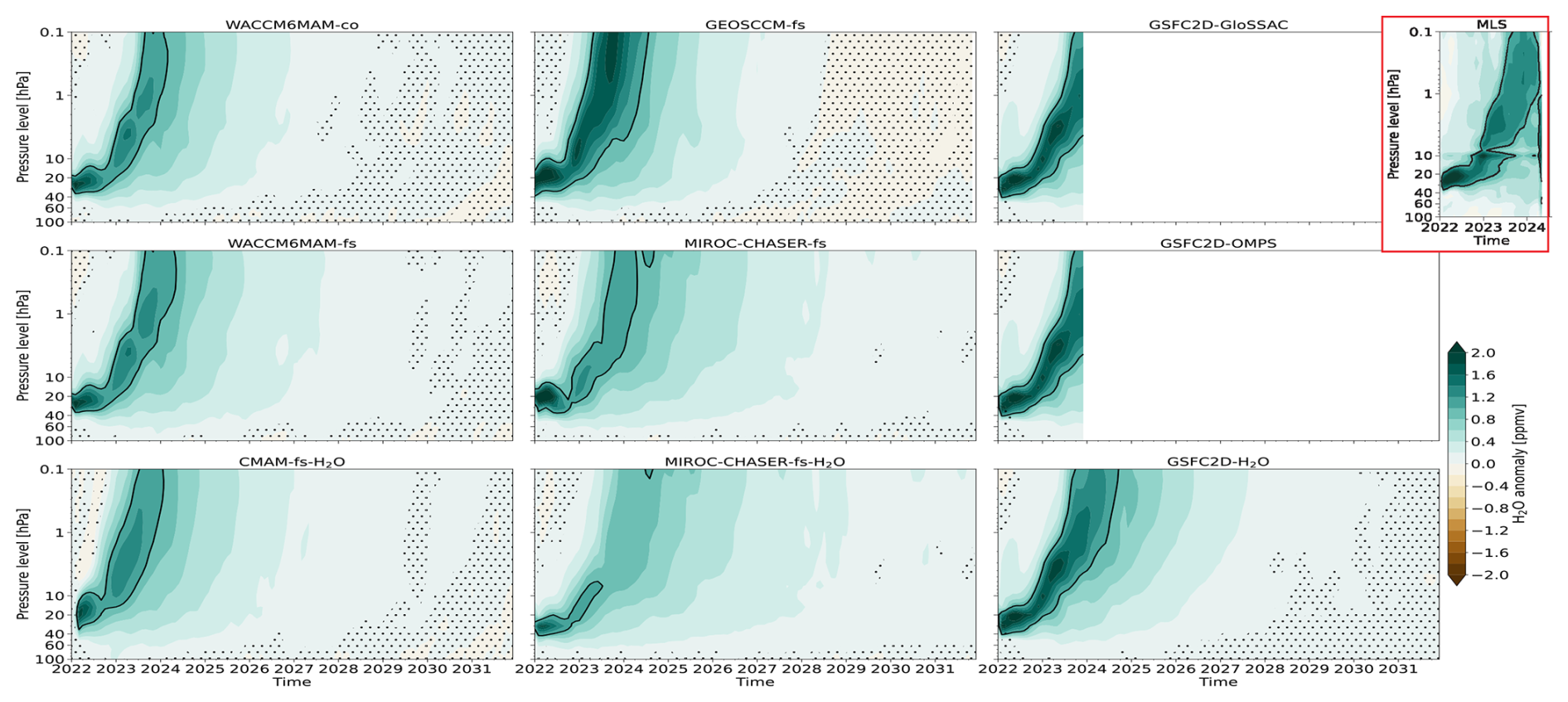
Figure 3 Simulated and observed (red inset box) global mean H₂O anomalies following the Hunga eruption. The modelled anomalies are relative to the control run. Dotted grids indicate statistically insignificant anomalies at the 95 % confidence level based on Student's t-tests. The solid black contours indicate an anomalous H₂O concentration of 1 ppmv.

The MLS anomaly is calculated relative to the 10-year climatology, and since the model anomalies are derived from Hunga eruption experiments relative to control runs without volcanic emissions, direct comparisons of detailed values are inappropriate. Therefore, our focus is on comparing the transport pattern. As shown in Fig. 3, all models successfully reproduce the three-phase transport pattern. Among them, WACCM6MAM–fs, WACCM6MAM–co, MIROC–CHASER–fs, and MIROC–CHASER–fs–H₂O exhibit slightly weaker upward transport, whereas GEOSCCM–fs, GSFC2D–GloSSAC, GSFC2D–OMPS, and GSFC2D–H₂O show slightly stronger upward transport compared to MLS. However, the differences among GSFC2D–GloSSAC, GSFC2D–OMPS, and GSFC2D–H₂O are quite small.

The three-phase transport pattern is also captured by the ICON–Seamless model in Niemeier et al. (2023), which simulated H₂O-only injection. That study highlighted that co-injection of SO₂ primarily affects the magnitude of vertical transport but does not alter the three-phase structure. This finding is further supported by comparisons between MIROC–CHASER–fs and MIROC–CHASER–fs–H₂O, as well as between GSFC2D–GloSSAC, GSFC2D–OMPS, and GSFC2D–H₂O.

In the long term, significant H₂O anomalies in the stratosphere and lower mesosphere are projected to persist for at least six years, until 2028, in WACCM6MAM–co. The longest projection indicates that a substantial anomaly could persist for over a decade, lasting until the end of the simulation in 2031, as indicated by MIROC–CHASER–fs and MIROC–CHASER–fs–H₂O. This prolonged anomaly may be attributed to a weaker upward transport, particularly in MIROC–CHASER–fs–H₂O, as indicated by both the anomaly pattern and the position of the 1 parts per million (ppmv) H₂O contour line. The extended H₂O lifetime in MIROC–CHASER–fs–H₂O, as shown in Fig. 1, further supports this conclusion.

3.3 Global-mean air temperature evolution

The upper atmospheric global-mean air temperature anomaly calculated from MLS data indicates slight warming in the lower stratosphere during 2022, particularly in the first half of the year (Fig. 4). Above this warming layer, strong cooling is observed in the middle and upper stratosphere, which extends into the lower mesosphere above 1 hPa from late 2022 onward.

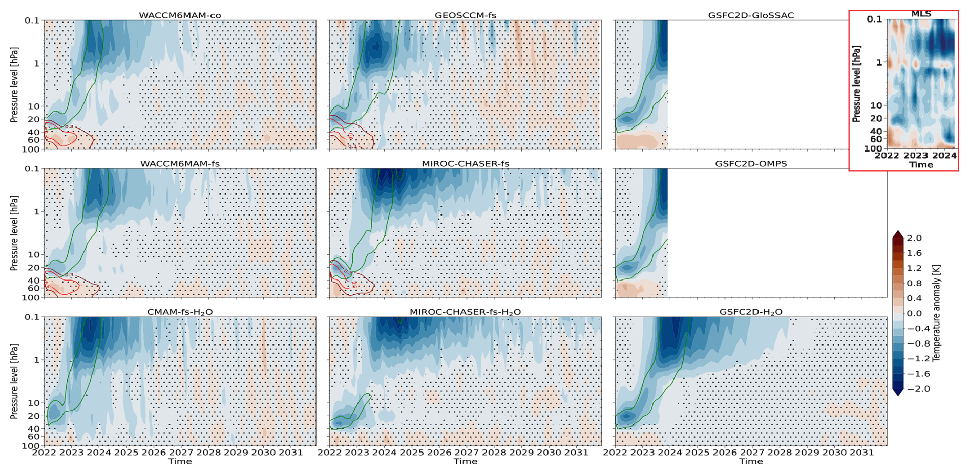
Figure 4 Simulated and observed (red inset box) global-mean air temperature anomalies following the Hunga eruption. The modelled anomalies are relative to the control run. Dotted grids indicate statistically insignificant anomalies at the 95 % confidence level based on Student's t-tests. Dark red and red contour lines denote modelled aerosol extinction coefficients at 0.3 and 0.6 × 10⁻³ km⁻¹, respectively, while dark green contour lines indicate modelled water vapor concentrations of 1 ppmv.

The upper-level cooling and lower-level warming dipole response pattern is reasonably reproduced by the model simulations, although with a smaller magnitude in most models compared to MLS. The significant cooling in the middle stratosphere (10–40 hPa) is more persistent than in the upper stratosphere (1–10 hPa), lasting between 3.5 and 4.5 years – until mid-2025 in WACCM6MAM–co and mid-2026 in GEOSCCM–fs. The strongest cooling is observed in the mesosphere above 1 hPa, where it persists for at least five years, until 2027, in GEOSCCM–fs and CMAM–fs–H₂O. This cooling persists even longer in simulations by WACCM6MAM, MIROC–CHASER, and GSFC2D, with the longest duration of up to 10 years observed in MIROC–CHASER–fs–H₂O. The modeled significant warming in the lower stratosphere is most prominent in 2022 in GEOSCCM–fs and MIROC–CHASER–fs. However, a more prolonged warming, extending into early and mid-2023, is observed in WACCM6MAM–co and WACCM6MAM–fs. This warming is also evident – and even stronger – in GSFC2D–GloSSAC and GSFC2D–OMPS.

The cooling observed in the middle and upper stratosphere corresponds to the ascent of H₂O, while the warming in the lower stratosphere is associated with the descent of aerosols that absorb solar near-infrared and terrestrial infrared radiation (Wang et al., 2023). Compared to MIROC–CHASER–fs, MIROC–CHASER–fs–H₂O exhibits stronger and more prolonged cooling in the middle stratosphere but less pronounced warming in the lower stratosphere. A similar pattern is observed when comparing GSFC2D–H₂O with GSFC2D–GloSSAC and GSFC2D–OMPS, where the former shows enhanced middle stratosphere cooling but weaker lower stratosphere warming. Although the greenhouse effect of stratospheric H₂O contributes to lower stratospheric warming, the significant warming is primarily driven by the co-injection of aerosols.

3.4 Global mean ozone variation

MLS data indicate ozone depletion in the lower stratosphere (20–100 hPa), an ozone increase in the middle stratosphere (around 10 hPa), and ozone depletion in the upper stratosphere (1–5 hPa), with the most pronounced depletion occurring in the lower mesosphere (0.1–1 hPa) in mid 2023–2024 (Fig. 5). This triple-response pattern – characterized by middle stratospheric ozone enhancement flanked by depletion above and below – is well captured by all model simulations, except for CMAM–fs–H₂O, which exhibits very limited ozone depletion in the lower stratosphere. However, the magnitude and timing of these ozone changes vary among models.

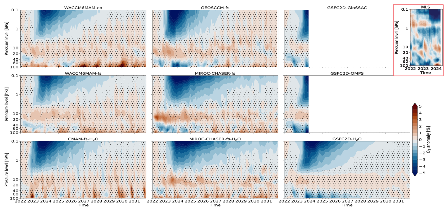
Figure 5 Simulated and observed (red inset box) global mean ozone anomalies following the Hunga eruption. The modelled anomalies are relative to the control run. Dotted grids indicate statistically insignificant anomalies at the 95 % confidence level based on Student's t-tests.

Among the simulations, all models project long-lasting ozone depletion in the lower mesosphere, persisting for at least 7 years. MIROC–CHASER–fs shows the most prolonged ozone depletion, extending to the end of the simulation (December 2031), and also exhibits the most pronounced ozone increase in the middle stratosphere, as well as an extended significant ozone depletion in the lower stratosphere between 2022 and 2025.

Compared to MIROC–CHASER–fs, MIROC–CHASER–fs–H₂O shows a smaller ozone increase in the middle stratosphere and less ozone depletion in the lower stratosphere. The significant ozone depletion between 20 and 40 hPa observed in GSFC2D–GloSSAC and GSFC2D–OMPS in 2022 is less pronounced in GSFC2D–H₂O. This highlights the crucial role of the co-injected SO₂ in driving ozone depletion in the lower stratosphere. These findings confirm the combined effect of both H₂O and SO₂, as discussed by Wang et al. (2023).

Ozone depletion in the lower stratosphere is driven by heterogeneous chlorine activation and enhanced dinitrogen pentoxide on hydrated aerosols (Evan et al., 2023; Zhang et al., 2024; Zhu et al., 2022, 2023). In contrast, ozone depletion in the lower mesosphere is linked to increased reactive hydrogen and a corresponding reduction in equilibrium ozone (Fleming et al., 2024; Randel et al., 2024), resulting from the upward transport of water vapor (Fig. 3), which leads to significant cooling (Fig. 4). The depleted ozone layer absorbs less ultraviolet (UV) radiation, further amplifying cooling at these altitudes. Consequently, stronger UV radiation enhances ozone production in the middle stratosphere, while ozone concentrations decrease above this layer. Furthermore, direct chemical effects lead to increased ozone in the mid-stratosphere. These impacts include the N₂O₅ + H₂O heterogeneous reaction on enhanced sulfate aerosols which reduces NOx and the odd nitrogen-ozone loss cycle, at least at altitudes where the aerosol is significant enough (Wilmouth et al., 2023; Santee et al., 2023; Zhang et al., 2024). The enhanced OH from the H₂O injection converts NO2 to the reservoir HNO₃, also reducing the odd nitrogen–ozone loss cycle in the mid-stratosphere (Fleming et al., 2024). Beyond the chemical feedback effects, the increase in ozone in the middle stratosphere is also influenced by transport changes associated with a weakening of the midlatitude Brewer-Dobson circulation (Wang et al., 2023).

The ozone response mechanisms discussed here draw on previous single-model studies that conducted detailed photochemical analyses using the same modeling frameworks. While the current study does not include new quantitative calculations of individual reaction rates or radiative effects, a dedicated multi-model analysis of the ozone response and its underlying mechanisms is currently underway.

4 Summary and Conclusions

The 2022 Hunga eruption was the most explosive volcanic event since the 1991 Pinatubo eruption. In contrast to Pinatubo, which injected a large amount of SO₂, Hunga released only ∼ 0.5 Tg of SO₂ but was distinguished by an unprecedented injection of ∼ 150 Tg of water vapor into the stratosphere, with some reaching the lower mesosphere. To investigate the evolution of SO₂ and H₂O perturbations and their subsequent atmospheric and climate impacts, the HTHH–MOC activity was endorsed by the WCRP APARC, fostering collaboration between the observational and modeling communities. In this study, we evaluate multi-model simulations against observations for the first two years, along with subsequent projections of their evolution, using Experiment 1, the only long-term simulation extending up to 10 post-eruption years. This assessment aims to evaluate the reliability of the models in capturing the evolution of volcanic emissions and predicting their impacts on temperature and ozone in the stratosphere and lower mesosphere.

Our results indicate that models successfully reproduce the latitudinal distribution of aerosols, which initially exhibit southward transport in the first year and reach Southern Hemisphere (SH) polar latitudes by the austral winter of 2023, reflecting the stratospheric transport dominated by the Brewer-Dobson circulation. Aerosols persist for approximately 2 years, with some models suggesting an additional 0.5 to 1.5 years of persistence in polar latitudes.

MLS observations show a plateau in H₂O mass between 1 and 70 hPa during the first year, followed by a continuous decline starting in late 2022. Models generally reproduce this plateau in 2022, with a subsequent sharp decline beginning in 2023. However, MIROC–CHASER–fs deviates by showing a shorter plateau, with a continuous decrease starting from mid-2022. The significant H₂O perturbation is projected to last four years (until 2026) in WACCM6MAM–co and 7 years (until 2029) in MIROC–CHASER–fs. The impact of this 4–7 years of stratospheric water vapor perturbation on stratospheric and lower mesospheric chemistry and dynamics remains an open question and requires further investigation. Understanding these effects is crucial for improving climate change detection and attribution in the coming years.

To comply with the experiment protocol, different models simulated H₂O injection using various methods and initial injection amounts, ranging from 150 Tg in WACCM6MAM–co and WACCM6MAM–fs to 750 Tg in GEOSCCM–fs. This variation in injection amounts results in differences in the maximum H₂O mass across models, which range from 139 Tg in WACCM6–MAM–fs to 166 Tg in GSFC2D–H₂O. The e-folding time is calculated based on the maximum mass rather than the initial injection amount, given the substantial differences in initial injection sizes. The estimated e-folding times range from the shortest at 31 months in GSFC2D–H₂O to the longest at 43 months in MIROC–CHASER–fs and MIROC–CHASER–fs–H₂O.

Both observations and model simulations indicate warming in the lower stratosphere and significant cooling above, accompanied by ozone depletion in the lower stratosphere, an ozone increase in the middle stratosphere, and severe ozone depletion in the upper stratosphere and lower mesosphere. The ozone depletion persists for at least seven years, with some model projections extending up to at least a decade. Comparisons between simulations with combined SO₂ and H₂O injection and those with H₂O-only injection reveal that the significant cooling and ozone depletion in the upper stratosphere and lower mesosphere result from the presence of excessive water vapor. Additionally, the co-injection of SO₂ with H₂O is necessary to reproduce the significant warming and ozone depletion in the lower stratosphere, albeit with a limited amount of SO₂ injection.

In conclusion, the models effectively reproduced the overall transport patterns of SO₂ and H₂O, with varying lifetimes projected across different models. They also reproduce the observed patterns of temperature and ozone variations following the eruption, albeit with differences in timescales and magnitudes. As the first study to utilize multi-model simulations of the Hunga eruption, this research provides valuable insights into the long-term evolution of Hunga-injected water vapor and aerosols, as well as their impacts on stratospheric temperatures and ozone. Furthermore, this study demonstrates the reliability of these model simulations in assessing the underlying physical and dynamical mechanisms and their potential atmospheric and climate impacts in the coming years.

Appendix A

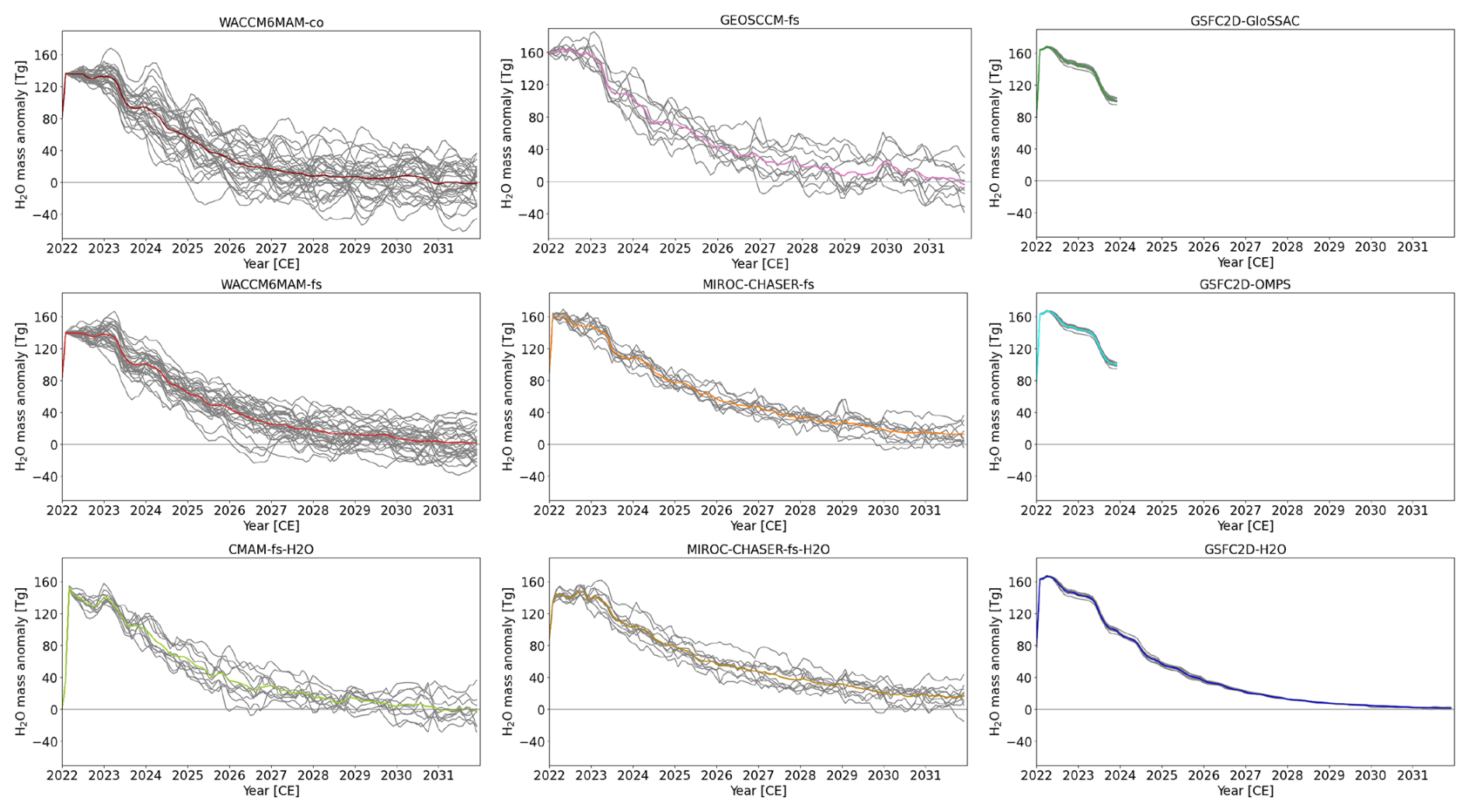
Figure A1 Simulated global stratospheric H₂O mass anomalies within the 1–70 hPa range following the Hunga eruption. Colored lines represent the ensemble mean anomalies relative to the control run, while gray lines indicate individual ensemble member anomalies.

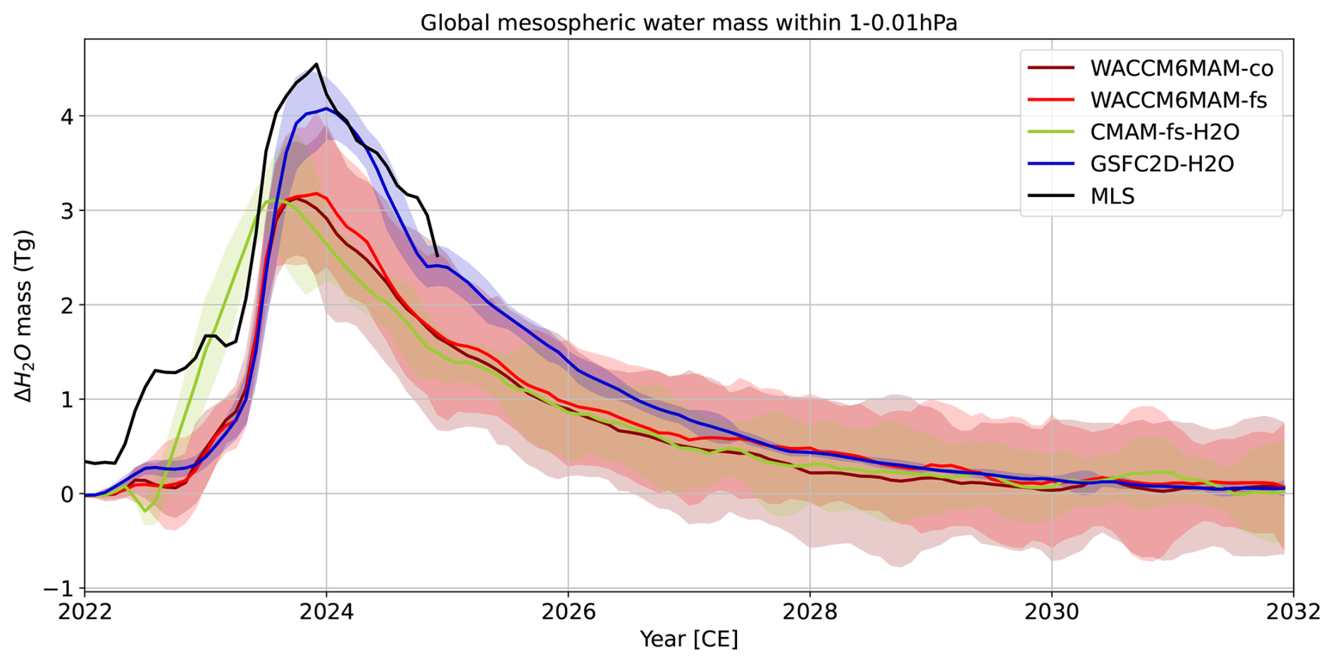
Figure A2 Simulated and observed global stratospheric H₂O mass anomalies within 1–0.01 hPa pressure range following the Hunga eruption. Colored lines show ensemble-mean anomalies relative to the control simulations for each model, with shading indicating the respective ensemble spreads. The black line represents the observed anomaly derived from Microwave Limb Sounder (MLS) water vapor measurements.

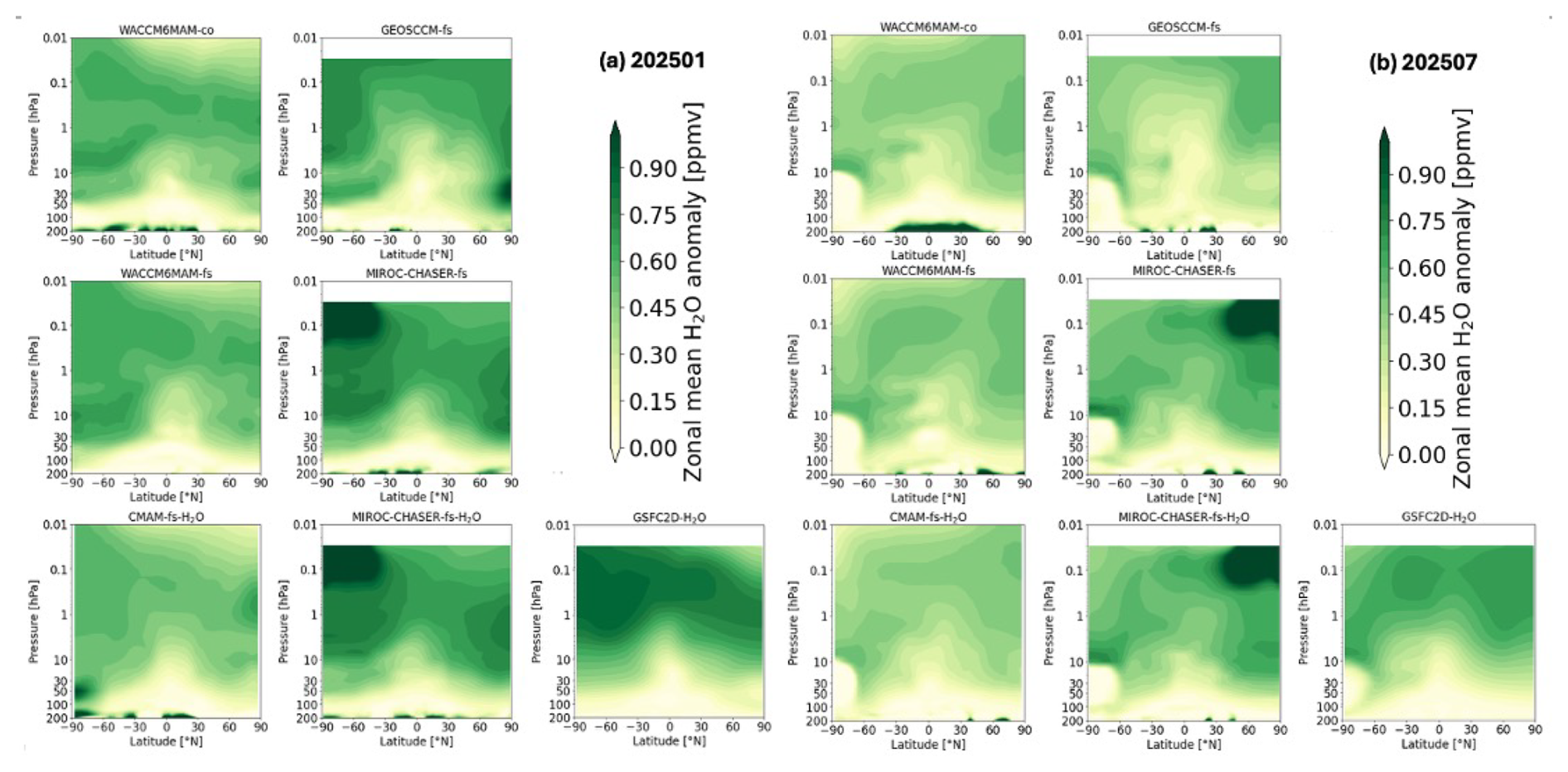
Figure A3 Latitude–pressure distribution of simulated zonal-mean water vapor anomalies in the upper atmosphere following the Hunga eruption, shown for (a) January 2025 and (b) July 2025. Anomalies are computed as differences between the ensemble mean of the experiment and control simulations.