Efficient use of a Lagrangian particle dispersion model for atmospheric inversions using satellite observations of column mixing ratios

Satellite instruments for measuring atmospheric column mixing ratios have improved significantly over the past couple of decades, with increases in pixel resolution and accuracy. As a result, satellite observations are being increasingly used in atmospheric inversions to improve estimates of emissions of greenhouse gases (GHGs), particularly CO₂ and CH₄, and to constrain regional and national emission budgets. However, in order to make use of the increasing resolution in inversions, the atmospheric transport models used need to be able to represent the observations at these finer resolutions. Here, we present a new and computationally efficient methodology to model satellite column average mixing ratios with a Lagrangian particle dispersion model (LPDM) and calculate the Jacobian matrices describing the relationship between surface fluxes of GHGs and atmospheric column average mixing ratios, as needed in inversions. The development will enable a more accurate representation of satellite observations (especially high-resolution ones) via the use of LPDMs and, thus, help improve the accuracy of emission estimates obtained by atmospheric inversions. We present a case study using this methodology in the FLEXPART (FLEXible PARTicle dispersion model) LPDM and the FLEXINVERT inversion framework to estimate CH₄ fluxes over Siberia using column average mixing ratios of CH₄ (XCH₄) from the TROPOMI (TROPOspheric Monitoring Instrument) instrument aboard the Sentinel-5P satellite. The results of the inversion using TROPOMI XCH₄ are evaluated against results using ground-based observations.

1 Introduction

Satellite remote sensing provides a wealth of information on the atmosphere and its composition. The number of satellite missions monitoring long-lived greenhouse gases (GHGs), specifically CO₂ and CH₄, has grown substantially over the past couple of decades, providing information on their variability, trends, and sources. From instruments aboard satellites, it is possible to retrieve mixing ratios of GHGs, most commonly as column averages (e.g. XCO₂ and XCH₄) or, depending on the instrument, viewing angle, and retrieval, as sub-columns, which can be used to derive estimates of surface–atmosphere fluxes using atmospheric transport models and inversion techniques (e.g. Alexe et al., 2015; Chen et al., 2023; Chevallier et al., 2005; Peiro et al., 2022; Zhang et al., 2023, 2021). Satellite instruments can be classified as “area flux mappers” or “point source imagers” (Jacob et al., 2022). Area flux mappers are high-precision instruments with larger pixel sizes (on the order of 0.1–10 km) and are designed to image mixing ratios on regional to global scales, whereas point source imagers have smaller pixel size (<0.1 km) and are designed to detect and quantify individual sources by mapping their plumes (Jacob et al., 2022). Specifically, it is the area flux mappers that are useful in inversions to estimate global and regional fluxes of CO₂ and CH₄, and they are becoming increasingly used to determine regional and national emission budgets and for comparisons with GHG emission inventories (e.g. Byrne et al., 2023; Deng et al., 2022; Maasakkers et al., 2021; Nesser et al., 2024; Worden et al., 2022). As satellite instrumentation has improved, there has also been an increase in pixel resolution. For example, the earliest satellite observations for CH₄ were from the SCIAMACHY instrument aboard ENVISAT, launched in 2002, which had a pixel size of 30 × 60 km, whereas the XCH₄ product from TROPOMI (TROPOspheric Monitoring Instrument) aboard Sentinel-5P, launched in 2017, has a pixel size at nadir of 5.5 × 7 km, and the recently launched MethaneSAT has a pixel size of just 0.1 × 0.4 km (Jacob et al., 2022). With this resolution increase, it is important to consider how the observations are represented in atmospheric transport models for inverse modelling.

Up to the present, inversions with satellite observations have primarily been made using Eulerian atmospheric transport models, either using Green's functions, adjoint models, or ensemble approaches to relate the column average mixing ratios to fluxes (e.g. Bergamaschi et al., 2009; Tsuruta et al., 2023; Varon et al., 2023). This is because the number of model iterations or ensemble members is independent of the number of observations, which for satellites can be a very large number. In contrast, there are only very few examples in the literature in which Lagrangian particle dispersion models (LPDMs) have been used with satellite observations (e.g. Ganesan et al., 2017; Wu et al., 2018) because the number of model calculations required in their backward mode is proportional to the number of observations making it computationally demanding.

On the other hand, LPDMs have some advantages over Eulerian models. LPDMs exhibit less numerical diffusion compared to Eulerian models; because of this, they generally better capture tracer filaments generated by atmospheric dispersion (Ottino, 1989) and fine structures in tracers mixing ratios resulting from long-range transport (Rastigejev et al., 2010). Furthermore, LPDMs can accurately represent any observation geometry, whereas an observation is represented by a grid cell in Eulerian models (Pisso et al., 2019). With the increasing resolution of satellite instruments, Eulerian model resolution may become a limiting factor in the ability to accurately represent an observation; hence, the use of LPDMs becomes a more interesting alternative. Finally, LPDMs can be run in a backward-in-time mode (without significant modifications to the code), which allows the sensitivity of an observation to fluxes to be calculated; in this way, LPDMs are sometimes said to be “self-adjoint”.

The main challenges of using LPDMs with satellite observations are (1) the number of observations for which backward computations need to be made and (2) that each retrieval is made over numerous vertical layers, which need to be represented in the model and combined with the retrieval's averaging kernel and prior mixing ratio profile. Here, we present a novel methodology to represent total column observations efficiently in an LPDM and to enable the use of LPDMs across a variety of spatial and temporal scales for atmospheric inversions with satellite data. The methodology has been implemented in the FLEXPART (FLEXible PARTicle dispersion model, version 10.4; Pisso et al., 2019) LPDM, but it could, in principle, be implemented in any LPDM. It can also be applied to any satellite retrieval.

We demonstrate the use of this methodology in a case study looking at CH₄ using retrievals from TROPOMI aboard the Sentinel-5P satellite. The case study region is Siberia, which was chosen because it has significant CH₄ emissions from both natural sources (e.g. peatlands) and anthropogenic sources (e.g. fugitive emissions from oil and gas extraction and transportation as well as from coal mining). We focus on the year 2020 and the months from March to October, for which there are an appreciable number of retrievals available. We use FLEXPART to model XCH₄ and, along with observed XCH₄, we derive estimates of CH₄ fluxes using the FLEXINVERT (Thompson and Stohl, 2014) Bayesian inversion framework. The fluxes from inversions using TROPOMI XCH₄ are evaluated via comparison with fluxes derived from inversions using ground-based observations from the JR-STATION (Japan–Russia Siberian Tall Tower Inland Observation Network) in situ measurement network (Sasakawa et al., 2010, 2012) as well as one in situ site and two flask sampling sites available form the World Data Centre for Greenhouse Gases (WDCGG).

2 Methodology

FLEXPART models atmospheric transport using virtual particles that are subject to transport and turbulent mixing as determined from meteorological fields. FLEXPART can be run in a backward-in-time mode, which is theoretically consistent with the forward-in-time-mode calculations (Flesch et al., 1995; Thomson, 1990), to calculate the residence time of virtual particles in a surface layer within the boundary layer and, thus, the influence of surface fluxes on these particles. In this mode, Jacobian matrices representing the influence of fluxes on an atmospheric observation can be derived, which are termed “source–receptor relationships” (SRRs), or sometimes “footprints” (Seibert and Frank, 2004). The SRRs can be integrated with flux fields to simulate mixing ratios and can be used in atmospheric inversions to update a prior estimate of the fluxes (e.g. Thompson and Stohl, 2014; Brioude et al., 2012). However, as far as we are aware, LPDMs have not been used before to model large numbers of satellite observations owing to the computational cost.

2.1 Modelling total column observations

Following Rodgers and Connor (2003), a modelled vertical profile x of mixing ratios can be compared with a retrieved profile using the following expression:

$$\begin{array}{}\text{(1)}& {\mathit{x}}^{\mathrm{sm}}={\mathit{x}}^{\mathrm{pri}}+\mathbf{A}\left(\mathit{x}-{\mathit{x}}^{\mathrm{pri}}\right),\end{array}$$

where A is the averaging kernel matrix (an N × N dimensional matrix), x^pri is the a priori profile used in the retrieval, and x^sm is a smoothed version of the vertical profile x. For a retrieval performed on N discrete pressure layers, the column average mixing ratio x^avg is the weighted sum of N sub-columns corresponding to the retrieval pressure layers (Apituley et al., 2021):

$$\begin{array}{}\text{(2)}& x^{\mathrm{avg}}=x^{\mathrm{avg},\mathrm{pri}}+\sum _{n=\mathrm{1}}^N{a}_n{w}_n{x}_n-\sum _{n=\mathrm{1}}^N{a}_n{w}_n{x}_n^{\mathrm{pri}},\end{array}$$

where x^avg,pri is the prior column average mixing ratio, a_n is the nth element of the column averaging kernel, w_n is a pressure-weighting term related to the thickness of the pressure layer, and x_n is the modelled mixing ratio for the nth retrieval layer. For LPDMs, x_n can be modelled as the product of the SRR for the nth retrieval layer H_n (a 1 × q dimensional matrix, where q is the number of flux variables) and the estimate of the fluxes f (q×1) as well as an estimate of the so-called “background” mixing ratio. Following Thompson and Stohl (2014), the background mixing ratio is modelled as the product of the background–receptor relationship (BRR) matrix calculated from the positions of the virtual particles when they terminate (${\mathbf{H}}_n^{\mathrm{ini}}$) and a 3D field of initial mixing ratios (yⁱⁿⁱ). Note that chemical losses during the backward-simulation period, e.g. from OH oxidation, can be taken into account in the SRR and BRR matrices. The modelled mixing ratio for the nth retrieval layer is thus

$$\begin{array}{}\text{(3)}& x_n={\mathbf{H}}_n\mathit{f}+{\mathbf{H}}_n^{\mathrm{ini}}{\mathbf{y}}^{\mathrm{ini}}.\end{array}$$

By substituting Eq. (3) into Eq. (2), we obtain the following:

$$\begin{array}{}\text{(4)}& \begin{array}{rl}{x}^{\mathrm{avg}}& =x^{\mathrm{avg},\mathrm{pri}}+\sum _{n=\mathrm{1}}^N{a}_n\left({\mathbf{H}}_n\mathit{f}{w}_n+{\mathbf{H}}_n^{\mathrm{ini}}{\mathit{y}}^{\mathrm{ini}}{w}_n\right)\\ & -\sum _{n=\mathrm{1}}^N{a}_n{w}_n{x}_n^{\mathrm{pri}}.\end{array}\end{array}$$

Thus, the column average SRR can be expressed as follows:

$$\begin{array}{}\text{(5)}& {\mathbf{H}}^{\mathrm{col}}=\sum _{n=\mathrm{1}}^N{a}_n{\mathbf{H}}_n{w}_n;\end{array}$$

a similar expression can be used for the column average BRR (H^col,ini).

Equations (2)–(5) represent the approach that has previously been used to model satellite observations with an LPDM, namely, the mixing ratio x_n has been calculated for each retrieval layer requiring calculation of the SRR H_n for each layer (Ganesan et al., 2017; Wu et al., 2018). Equation (5) requires the maintenance of information about each retrieval layer in order to calculate the column SRR. Our method (as described below) departs from this approach and is much more computationally efficient.

In FLEXPART (and LPDMs generally), SRRs are calculated by sampling the particles on a regular 3D grid. In general, for a grid cell i, the SRR for retrieval layer n is calculated as follows:

$$\begin{array}{}\text{(6)}& {\mathbf{H}}_{i,n}={\displaystyle \frac{\mathrm{1}}{P_n}}\sum _{p=\mathrm{1}}{\displaystyle \frac{l_{p,i,n}\mathrm{\Delta }{t}_{p,i,n}}{{\mathit{\rho }}_i}},\end{array}$$

where $l_{p,i,n}$ is the transmission function for particle p (and represents the fraction of the mass remaining in the particle, which can change after release in the case of atmospheric chemistry), $\mathrm{\Delta }{t}_{p,i,n}$ is the residence time of the particle in the grid cell, ρ_i is the air density in the grid cell, and P_n is the number of particles released in layer n (Seibert and Frank, 2004). (Note that, in Eq. 6, the number of particles summed over is not specified, as this depends on the number of particles that reside in the grid cell i and is ≤P_n.) Thus, the column SRR relationship is found by substituting Eq. (6) into Eq. (5):

$$\begin{array}{}\text{(7)}& {\mathbf{H}}_i^{\mathrm{col}}={\displaystyle \frac{\mathrm{1}}{{\mathit{\rho }}_i}}\sum _{n=\mathrm{1}}^N{a}_n{w}_n{\displaystyle \frac{\mathrm{1}}{P_n}}\sum _{p=\mathrm{1}}{l}_{p,i,n}\mathrm{\Delta }{t}_{p,i,n}.\end{array}$$

However, using Eq. (7) would still require the maintenance of information about which retrieval layer a particle had originated from in order to calculate the column SRR; furthermore, if P_n has the same value for all layers, this would mean that all layers are sampled equally, even though particles originating in upper layers are much more unlikely to reach the surface layer and, thus, contribute to the SRR.

Instead, we carry the information of a_nw_n by varying the particle density in each layer, where the number of particles released per layer, P_n, is as follows:

$$\begin{array}{}\text{(8)}& P_n=P{a}_n{w}_n,\end{array}$$

where P is the total number of particles released per retrieval. By substituting a_nw_n for $P_n/P$ into Eq. (7), we derive the following:

$$\begin{array}{}\text{(9)}& {\mathbf{H}}_i^{\mathrm{col}}={\displaystyle \frac{\mathrm{1}}{{\mathit{\rho }}_i}}{\displaystyle \frac{\mathrm{1}}{P}}\sum _{n=\mathrm{1}}^N\sum _{p=\mathrm{1}}{l}_{p,i,n}\mathrm{\Delta }{t}_{p,i,n}.\end{array}$$

Equation (9) can be simplified further by noting that the sum over N layers and the sum over particles in the grid cell i originating from each layer is equivalent to summing over the particles in the grid cell originating from all layers (hence we omit the index n):

$$\begin{array}{}\text{(10)}& {\mathbf{H}}_i^{\mathrm{col}}={\displaystyle \frac{\mathrm{1}}{{\mathit{\rho }}_i}}{\displaystyle \frac{\mathrm{1}}{P}}\sum _{p=\mathrm{1}}{l}_{p,i}\mathrm{\Delta }{t}_{p,i}.\end{array}$$

In Eq. (10), the information on the retrieval layer from which a particle originated does not need to be kept (as it is taken into account at the particle initialization via P_n), and the equation is analogous to that for point observations. This implementation was compared to calculating the SRRs for each layer individually, and the results were the same within the limits of numerical rounding errors. However, by implementing the calculation this way, total column observations can be simulated with the same computational cost as that for point observations.

Similarly, the total column BRR for the grid cell i can be obtained as follows:

$$\begin{array}{}\text{(11)}& {\mathbf{H}}_i^{\mathrm{col},\mathrm{ini}}={\displaystyle \frac{\mathrm{1}}{P}}\sum _{p=\mathrm{1}}{l}_{p,i}.\end{array}$$

A further consideration when modelling satellite observations with a Lagrangian model is the geometry of the retrieval, as the ground-based pixels are not necessarily rectangular and can be rotated with respect to the meridians and parallels. In FLEXPART (and LPDMs generally), an observation is represented by releasing virtual particles from a volume in which the particles are distributed randomly. However, the default is that this volume is rectangular and aligned with the meridians and parallels. Therefore, we have implemented an affine transformation on the particle positions so that the volume which they represent matches the geometry of the retrieval (see the Supplement for a complete description of the affine algorithm).

2.2 Averaging of retrievals

Even with the efficient modelling of total column measurements using the method described above, current satellite missions can provide on the order of 10 000 to 100 000 retrievals globally per day, making the cost of computing backward trajectories for each retrieval still computationally expensive if the study region is large. For this reason, we average the retrievals to so-called “super-observations”. Averaging retrievals also has the advantage that the random error in the super-observation is reduced compared to each individual retrieval.

However, in some areas where there is strong heterogeneity in the column average measurements, for instance, due to large localized sources, it would be advantageous to keep higher-resolution observations. Therefore, we developed an optimal averaging routine in which the degree of averaging is based on the standard deviation of the column average mixing ratios. The retrievals are averaged to rectangular grid cells that are aligned with the meridians and parallels. The user decides on the finest resolution grid cell to be used (d_min) and the number of resolution steps (nsteps). The averaging is first performed for the coarsest resolution (given as $d_{\min }\times {\mathrm{2}}^{\mathrm{nsteps}-\mathrm{1}}$) and is then refined stepwise (from nsteps −1 to 0) by dividing grid cells into four where the standard deviation (recalculated at each step) is above a given threshold. If there are any quarters of the grid cell (as defined for the current step) where there are no retrievals, the grid cell is divided in the next iteration anyway to avoid having a super-observation for a grid cell that is not fully represented by the retrievals. Retrievals that are outside ±2 standard deviations of the grid cell mean are not included in the average to avoid influence from large outliers. The averaging is redefined each day based on the available retrievals.

In the algorithm, the column average mixing ratio corresponding to the average of M retrievals is calculated as follows:

$$\begin{array}{}\text{(12)}& \stackrel{\mathrm{‾}}{x}={\displaystyle \frac{\mathrm{1}}{S}}\sum _{m=\mathrm{1}}^M\left(s_m{x}_m^{\mathrm{pri}}+\sum _{n=\mathrm{1}}^N{s}_m{a}_{m,n}{w}_{m,n}\left(x_{m,n}-x_{m,n}^{\mathrm{pri}}\right)\right),\end{array}$$

where $\stackrel{\mathrm{‾}}{x}$ is the total column mixing ratio corresponding to the average, $x_m^{\mathrm{pri}}$ is the prior column average mixing ratio of the mth retrieval, N is the number of vertical layers in the retrievals, s_m is the surface area, and S is the total surface area of all retrievals. By rearranging Eq. (12), we obtain the following:

$$\begin{array}{}\text{(13)}& \begin{array}{rl}\stackrel{\mathrm{‾}}{x}& ={\displaystyle \frac{\mathrm{1}}{S}}\sum _{m=\mathrm{1}}^M{s}_m{x}_m^{\mathrm{pri}}+{\displaystyle \frac{\mathrm{1}}{S}}\sum _{m=\mathrm{1}}^M\sum _{n=\mathrm{1}}^N{s}_m{a}_{m,n}{w}_{m,n}{x}_{m,n}\\ & -{\displaystyle \frac{\mathrm{1}}{S}}\sum _{m=\mathrm{1}}^M\sum _{n=\mathrm{1}}^N{s}_m{a}_{m,n}{w}_{m,n}{x}_{m,n}^{\mathrm{pri}},\end{array}\end{array}$$

and this can be written as

$$\begin{array}{}\text{(14)}& \begin{array}{rl}\stackrel{\mathrm{‾}}{x}& =\stackrel{\mathrm{‾}}{x^{\mathrm{pri}}}+\sum _{n=\mathrm{1}}^N\stackrel{\mathrm{‾}}{x_n}\stackrel{\mathrm{‾}}{a_n{w}_n}-{\displaystyle \frac{\mathrm{1}}{S}}\sum _{m=\mathrm{1}}^M\sum _{n=\mathrm{1}}^N{s}_m{a}_{m,n}{w}_{m,n}{x}_{m,n}^{\mathrm{pri}}\\ & \left(\text{if}\mathrm{all}{x}_{m,n}=\stackrel{\mathrm{‾}}{x_n}\right),\end{array}\end{array}$$

where $\stackrel{\mathrm{‾}}{x^{\mathrm{pri}}}$ is the area-weighted average prior column mixing ratio, and $\stackrel{\mathrm{‾}}{a_n{w}_n}$ and $\stackrel{\mathrm{‾}}{x_n}$ are, respectively, area-weighted average column averaging kernel and pressure weighting and the mixing ratio corresponding to the nth layer. Note that the condition “if all $x_{m,n}=\stackrel{\mathrm{‾}}{x_n}$” is met when the particle release is made for the area over which the M retrievals are averaged. The uncertainty in the super-observation is calculated as the quadratic sum of the uncertainties in the individual retrievals weighted by the ground-pixel area of the retrievals.

For FLEXPART users, we include a description of the changes to the v10.4 code for the implementation of this methodology in the Supplement. In addition, we include a brief description of how these developments could be used with the recently released FLEXPART v11.

3 Case study on methane sources in Siberia

We demonstrate the use of FLEXPART for modelling column average mixing ratios, as well as the averaging algorithm, in a case study looking at CH₄ emissions in Siberia. Siberia was chosen because it is a region with significant CH₄ emissions from both natural sources (e.g. peatlands) and anthropogenic sources (e.g. fugitive emissions from oil and gas extraction and transportation as well as from coal mining). It was also in Siberia that one of the largest point source emissions of CH₄ was detected by GHGSat (from a coal mine in the Kemerovo region; https://www.bbc.com/news/science-environment-61811481, last access: 17 September 2025), and significant CH₄ sources have also been detected in this region by TROPOMI (Trenchev et al., 2023). On the other hand, Siberia is a challenging region to study, as there are no observations available north of around 50° N in the winter and the region is often cloudy, further limiting the number of available retrievals. Our inversion domain covers western and central Siberia (50– to 115° E and 40–80° N) and includes the West Siberian Plain, major oil and gas fields, and important coal mining regions such as Kemerovo (Fig. 1). We limit the period of our study to March to October – months during which there are observations available north of 50° N – and focus on the year 2020.

To evaluate the inversions using TROPOMI XCH₄, we make use of the JR-STATION ground-based network of CH₄ measurements. JR-STATION consists of nine sites with in situ measurements of CH₄, with the first sites having data from 2004 (Sasakawa et al., 2010, 2012).

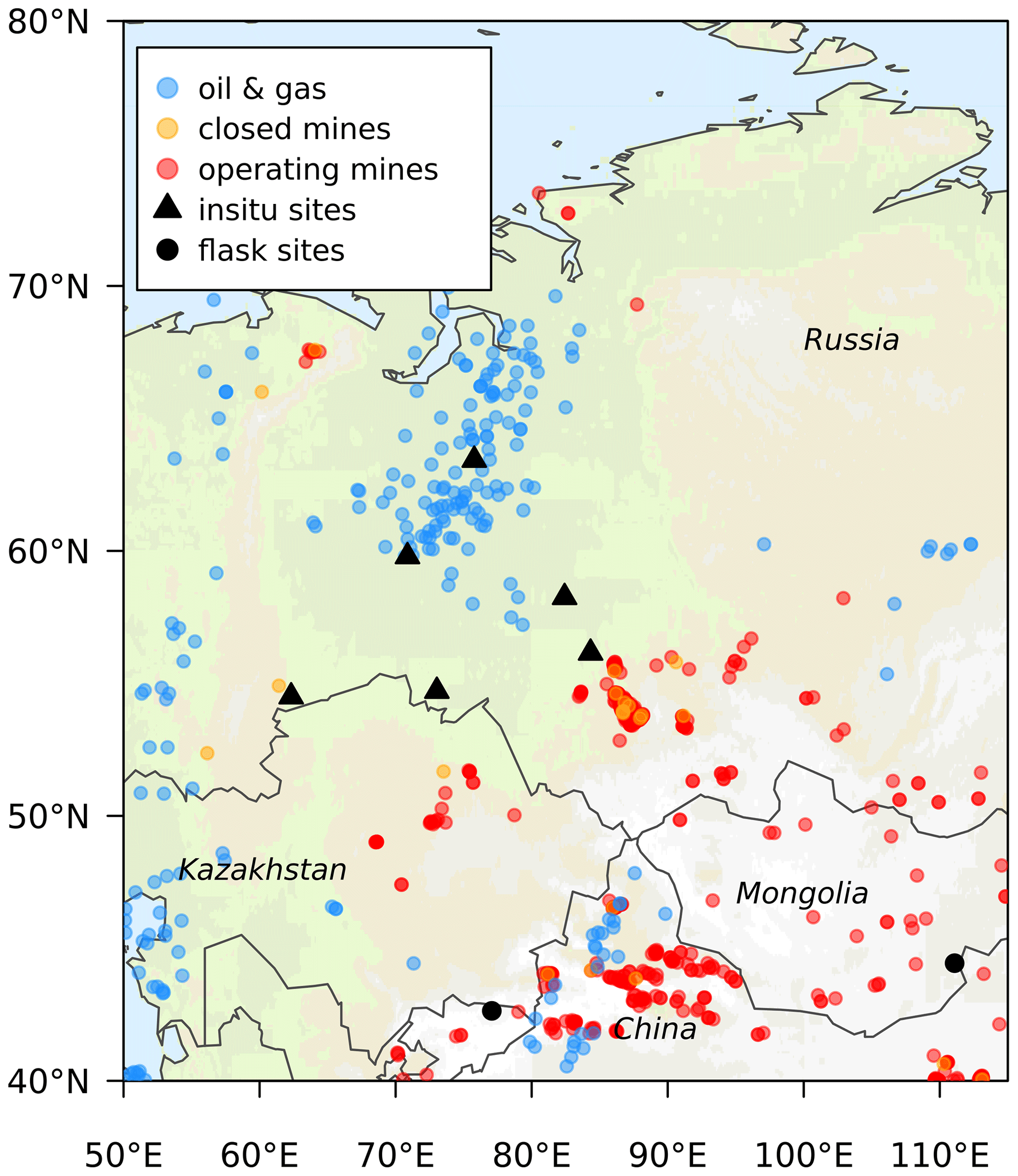
Figure 1 Map of the inversion domain indicating oil and gas extraction and coal mining locations and the ground-based sites used in the inversion. The oil and gas and the coal mining data were obtained from Global Energy Monitor (https://globalenergymonitor.org, last access: 17 September 2025).

3.1 Case study methodology

3.1.1 Inversion method

For the inversion, we use the FLEXINVERT Bayesian inversion framework as described by Thompson and Stohl (2014). In this framework, the optimal fluxes are those that minimize the cost function:

$$\begin{array}{}\text{(15)}& \begin{array}{rl}J\left(\mathit{z}\right)& ={\displaystyle \frac{\mathrm{1}}{\mathrm{2}}}{\left(\mathit{z}-{\mathit{z}}_b\right)}^{\mathrm{T}}{\mathbf{B}}^{-\mathrm{1}}\left(\mathit{z}-{\mathit{z}}_b\right)+{\displaystyle \frac{\mathrm{1}}{\mathrm{2}}}{\left(\mathbf{H}\mathit{z}-\mathit{y}\right)}^{\mathrm{T}}\\ & {\mathbf{R}}^{-\mathrm{1}}\left(\mathbf{H}\mathit{z}-\mathit{y}\right),\end{array}\end{array}$$

where B is the prior error covariance matrix and describes the error and error correlation of the prior fluxes, R is the observation error covariance matrix and describes the uncertainty in the observations, z_b is the prior state vector, z is the optimal (or posterior) state vector, and y is the observation vector. The minimum of the cost function is found using the M1QN3 quasi-Newton algorithm (Gilbert and Lemaréchal, 1989). This algorithm does not provide an estimate of the Hessian matrix ∇²J(z); therefore, the posterior uncertainty was calculated instead using a Monte Carlo ensemble, following Chevallier et al. (2007).

The state vector variables include offsets to the prior fluxes, which are resolved at a 14 d temporal resolution and at varying spatial resolutions from 0.5 to 2.0°, depending on how strongly the fluxes influence the observations (Thompson and Stohl, 2014). The spatial resolution of the state vector was calculated separately for the TROPOMI and for the ground-based observations (see Supplement Fig. S1 for maps of the spatial grid). For each 14 d interval, this resulted in 2619 flux variables for the TROPOMI inversions and 5920 flux variables for the ground-based observation inversions. Note that only land fluxes were optimized in the inversions, as the observations have little sensitivity to fluxes over the ocean. In any case, the contribution from ocean fluxes to the modelled mixing ratios was accounted for (only these fluxes were fixed to the prior values and not optimized). The state vector also includes scalars of the boundary conditions (i.e. the initial mixing ratios in 3D space represented by the vector yⁱⁿⁱ in Eq. 3). The scalars are defined for four latitudinal bands, 90–30° N, 30–0° N, 0–30° S, and 30–90° S, and for three vertical layers, from 0 to 2000, 2000 to 10 000, and 10 000 to 70 000 m a.g.l. (above ground level), and are optimized for 28 d averages. The uncertainty in the scalars was set at 5 % for the TROPOMI inversions and at 1 % for the ground-based observation inversions. A larger uncertainty was chosen for the TROPOMI inversions after initial tests showed that lower uncertainties did not allow sufficient freedom to correct erroneous prior background mixing ratios (see Sect. 3.2.2).

For the case study, FLEXPART was run using the European Centre for Medium-Range Weather Forecasts (ECMWF) ERA5 meteorological reanalysis data at a 0.5° × 0.5° and hourly resolution. Backward trajectories were made using 30 000 particles for each TROPOMI super-observation. The trajectories were calculated for 20 d backward in time from the time of the observation. The SRRs were calculated at 0.5° over the inversion domain and at 2.0° globally. In addition, the BRR (${\mathbf{H}}_n^{\mathrm{ini}}$ in Eq. 3) was calculated at the termination of the particles. For comparison with the inversions using TROPOMI retrievals, we also performed inversions using ground-based observations. The FLEXPART runs for these observations used the same set-up as that for the retrievals but with only 20 000 particles per observation, which was deemed sufficient to represent a point observation.

The so-called background mixing ratio for each column average observation was calculated as H^col,iniyⁱⁿⁱ (see Eqs. 3–5), where yⁱⁿⁱ is a 3D field of CH₄ mixing ratios (resolved daily) and was taken from the Copernicus Atmosphere Monitoring Service (CAMS) data assimilation product, EGG4 (https://ads.atmosphere.copernicus.eu/datasets/cams-global-ghg-reanalysis-egg4?tab=overview, last access: 17 September 2025). In addition, we have used 3D mixing ratio fields from the CAMS greenhouse gas inversion product TM5-4DVAR (https://atmosphere.copernicus.eu/greenhouse-gases-supplementary-products, last access: 17 September 2025) in a sensitivity test.

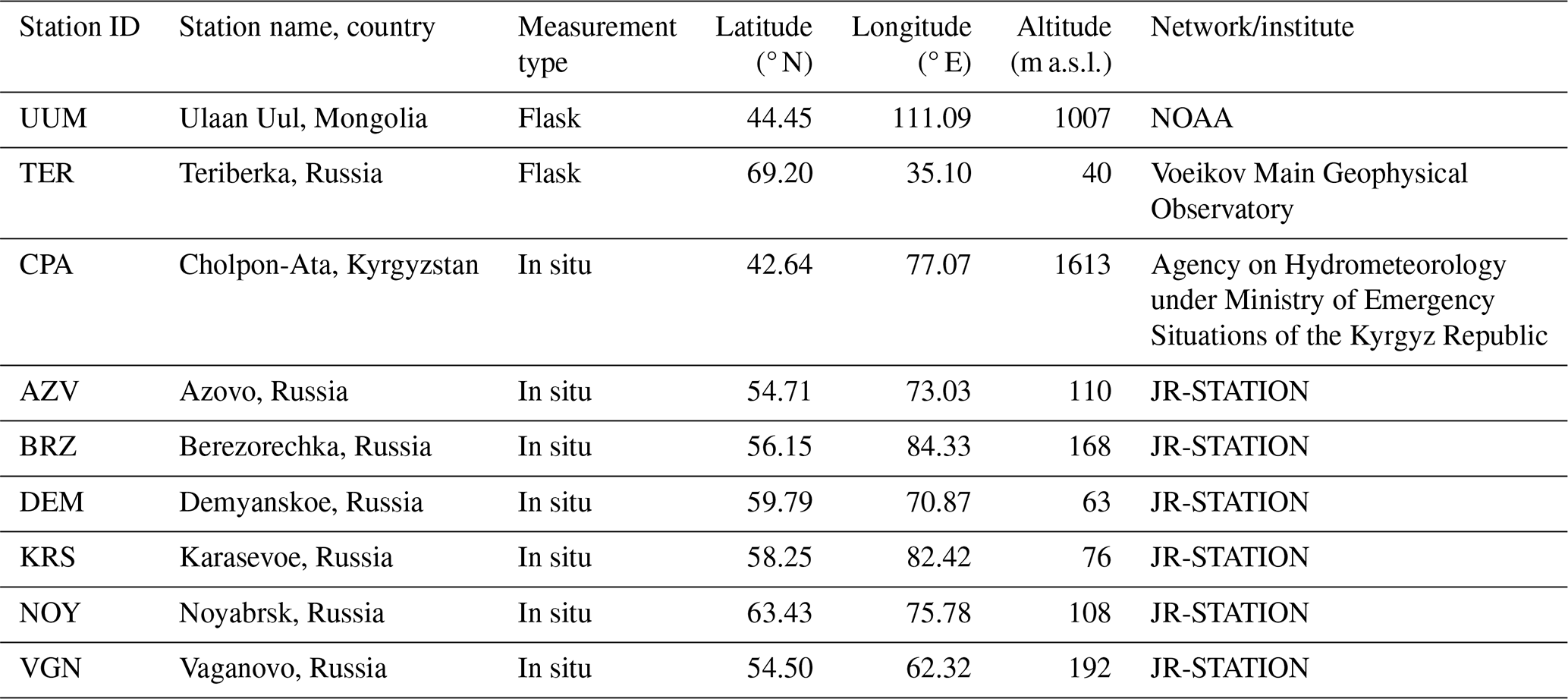
Table 1 Ground-based atmospheric observation sites. The altitude refers to that of the air intake.

3.1.2 Observations

In this case study, we use the Weighting Function Modified Differential Optical Absorption Spectroscopy (WFMD) retrieval product (version 1.8) from the University of Bremen (Schneising et al., 2019, 2023). We selected retrievals that had a quality flag of 0 (where the quality value is either 0 (good) or 1 (bad)). The retrievals were averaged to super-observations, as described in Sect. 2.2, using two resolution steps with grid cell sizes of 0.25 and 0.5°. Uncertainties for the super-observations were calculated as the quadratic sum of the uncertainty for each retrieval weighted by the area of the ground pixel of the retrieval. The full observation-space uncertainty was the quadratic sum of the super-observation uncertainty and an uncertainty estimated for the background column average mixing ratio. The resulting observation-space uncertainties were typically in the range of 14–20 ppb with a median value of 16 ppb. The square values of these uncertainties were used as the variances in the observation error covariance matrix, and we assumed that errors in the super-observations were uncorrelated. On average, there were 3781 super-observations per day (see Fig. S2 for an overview of the number of super-observations by latitude and state vector time step).

For validation, we used ground-based observations from the JR-STATION network (Sasakawa et al., 2010, 2012, 2025) (Fig. 1 and Table 1). It is comprised of nine (currently six operating) tower sites in Siberia where simultaneous multi-point semi-continuous observations of CO₂ and CH₄ have been made. The CH₄ mixing ratios were measured using a modified SnO₂ semiconductor sensor and determined against the NIES 94 CH₄ scale. The NIES 94 CH₄ scale ranges approximately 5 ppb higher than the WMO-CH4-X2004A scale; thus, we adjusted the CH₄ mixing ratios to the WMO scale for use in the inversions. The JR-STATION system measures the air at each intake height on the tower for 3 min at a time before switching the airflow to the next height. The 3 min values for each height are averaged to obtain a representative value for each hour. In addition, we used observations from the flask sampling sites Ulaan Uul in Mongolia (UUM) and Teriberka in Russia (TER) and in situ observations from the Global Atmospheric Watch site Cholpon-Ata in Kyrgyzstan (CPA), which were all obtained from the World Data Centre for Greenhouse Gases (WDCGG). These data were filtered to remove observations that were flagged as “invalid”, and for the flask data, pairs of flasks were averaged to one observation. The observation-space uncertainties were typically in the range of 11–14 ppb with a median value of 12 ppb.

Table 2 Overview of flux estimates used in the prior.

3.1.3 Prior information

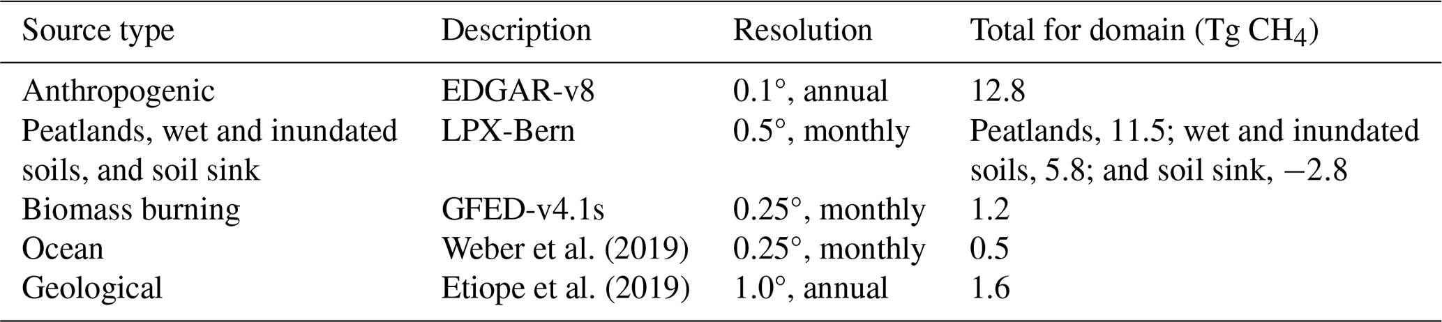
In the case study inversion, we optimize the total net CH₄ flux. A prior estimate for the total net flux was prepared using the following input datasets: (i) EDGAR-v8 for anthropogenic emissions (Crippa et al., 2023); (ii) the LPX-Bern land-surface model for natural fluxes from peatlands, wet and inundated soils, and the soil sink; (iii) Etiope et al. (2019) for geological emissions; (iv) GFED-v4.1s for biomass-burning emissions (van der Werf et al., 2017); and (v) the observation-based climatology of Weber et al. (2019) for ocean fluxes. An overview of the flux estimates used in the prior is given in Table 2. The input data are given at different temporal and spatial resolutions and, thus, were averaged/interpolated to the same spatial resolution as the SRRs for the inversion domain, i.e. 0.5° and interpolated to 14 d to match the state vector temporal resolution.

For the inversion using ground-based observations, prior uncertainties were calculated for each grid cell as 50 % of the prior estimate but with a lower limit of $\mathrm{1}\times {\mathrm{10}}^{-\mathrm{9}}$ kg m⁻² h⁻¹, which is approximately the 10th percentile value of all fluxes over the inversion domain. For the inversions using TROPOMI, after a first inversion was run with the same uncertainties as for the ground-based inversion, and which showed very little change in the posterior versus the prior fluxes, the prior uncertainty was increased to 100 %. The prior error covariance matrix, B, was calculated using the square of the prior uncertainties in each grid cell as the variances and the co-variances were calculated assuming that the correlation between two grid cells decays exponentially with a correlation scale length of 200 km, and the correlation between flux time steps decays exponentially with a correlation scale length of 28 d.

3.2 Results and discussion

3.2.1 Inversion diagnostics

The TROPOMI inversion was run for 25 iterations, whereas the ground-based observation inversion was run for 30 iterations. For the TROPOMI inversions, 25 iterations was deemed a sufficient number for convergence based on the change in the cost at each iteration, which was <1 % after 17 iterations. For the ground-based observation inversion, the change in cost was only consistently <1 % after 23 iterations (the cost at each iteration for both inversions is shown in Fig. S3).

Another inversion diagnostic that is often used to determine the appropriateness of the state space and observation-space uncertainties is the reduced chi-square value, which is twice the final cost (see Eq. 14) divided by the number of degrees of freedom, which has an expected value of 1 (Tarantola, 2005). However, the reduced chi-square criterion can be ambiguous, as pointed out by Chevallier et al. (2007). In any case, here we report the reduced chi-square values for the TROPOMI and ground-based inversions, which were 1.08 and 2.16, respectively.

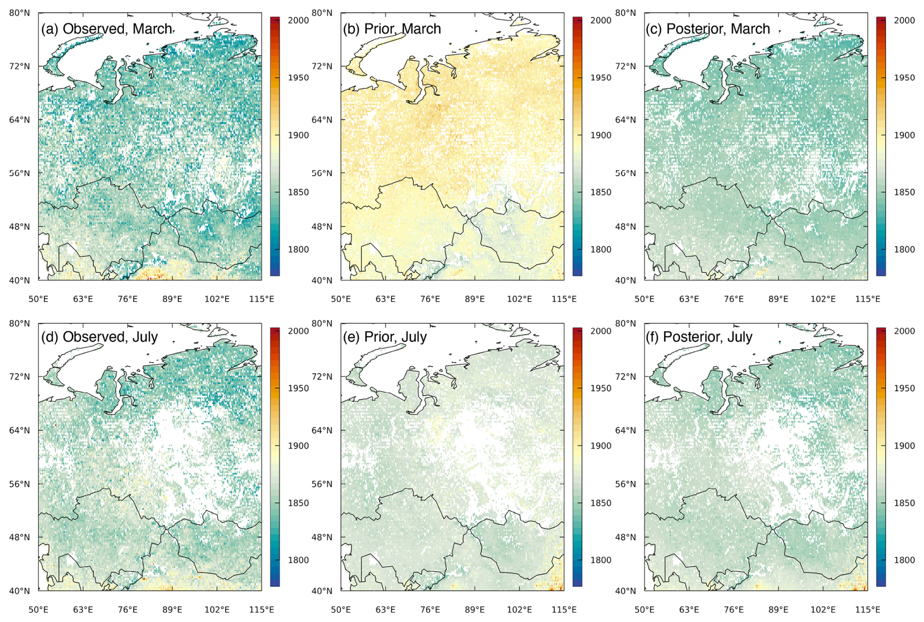
Figure 2 Monthly mean XCH₄ from super-observations (in ppb) for March 2020 from (a) observations, (b) modelled values using prior fluxes, and (c) modelled values using posterior fluxes and scalars of initial mixing ratios. Panels (d) to (f) are the same as panels (a) to (c) but for the monthly mean XCH₄ for July 2020. Note that, for plotting, the super-observations were averaged to a regular grid of 0.25°.

3.2.2 Modelled XCH₄

Column mixing ratios of CH₄ were modelled for each of the super-observations using the set-up described above. The observations for all months show high XCH₄ values for the southern part of the domain, especially in northern China. This is also captured, although with lesser magnitude, in the prior and posterior modelled XCH₄ (Fig. 2). In the summer months (June–August), there is also elevated XCH₄ in the central part of the domain, corresponding to the location of wetlands as well as to oil and gas fields. The posterior modelled XCH₄ had a much closer agreement with the observations, as expected. For example, for March, the a posteriori mean error (ME) and root-mean-square error (RMSE) were 2 and 16 ppb, respectively, compared to corresponding a priori values of 45 and 50 ppb. For July, the a posteriori ME and RMSE were 3 and 13 ppb, compared to a priori values of 12 and 20 ppb. The differences between the posterior and prior modelled XCH₄ are shown in Fig. S4.

The generally too high modelled XCH₄ using the prior state vector, especially in March, was primarily due to a too high background estimate when this was based on initial mixing ratios from EGG4. Further simulations using the CAMS greenhouse gas inversion product (CAMSv20r1) showed that the modelled XCH₄ is strongly sensitive to the fields of the initial mixing ratio used, and the prior modelled XCH₄ was considerably lower using CAMSv20r1 (see Fig. S5). The reason for this is the different vertical distributions of CH₄ in CAMSv20r1 versus EGG4 (see Fig. S6), which convolved with the averaging kernel and the FLEXPART-calculated averaging matrix H^ini,col lead to quite different values for the background column average mixing ratio. A bias is also seen when XCH₄ is calculated directly from the initial mixing ratio fields (by applying Eq. 2), with EGG4 resulting in significantly higher and CAMSv20r1 resulting in significantly lower XCH₄ compared to the observations in March, although with smaller biases in July (see Fig. S7). For this reason, the boundary conditions (i.e. 3D fields of initial mixing ratios) are optimized in the inversion simultaneously with the fluxes.

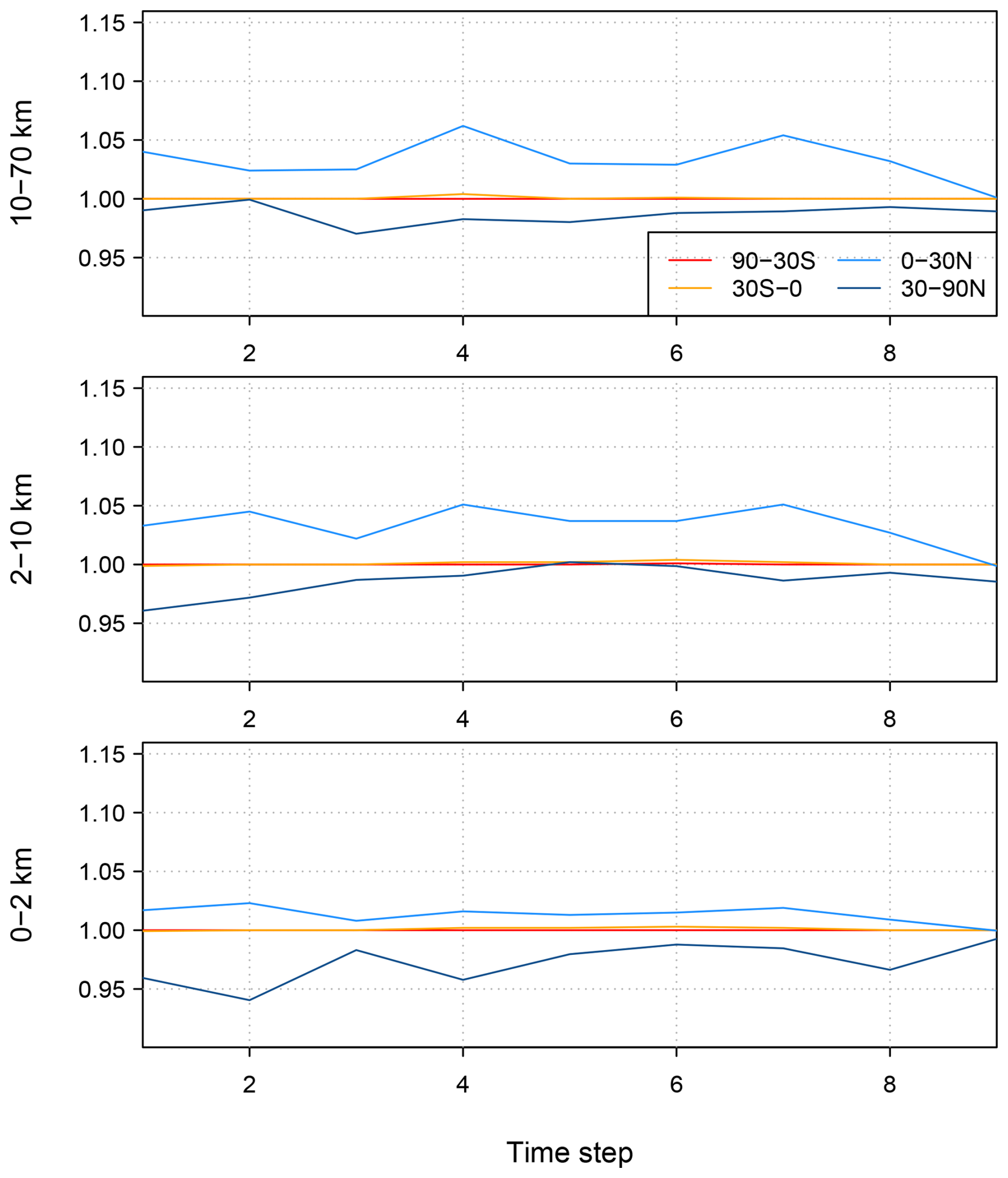
Figure 3 Posterior scalars of the initial mixing ratios from the TROPOMI inversion using 3D initial mixing ratio fields from EGG4. In each sub-panel, the scalars are shown for each time step of 28 d and for each of the four latitude bands.

In the inversion using EGG4, the posterior scalars of initial mixing ratios were decreased in the latitude band 30–90° N at all altitude layers and time steps, the mixing ratios in the 0–30° N band were increased slightly in the lowest altitude layer and more strongly in the upper two layers, and the scalars for the Southern Hemisphere did not differ significantly from the prior value of 1.0 (Fig. 3). In contrast, in the inversion using CAMSv20r1, the scalars for 30–90° N were decreased only for the lowest altitude layer, remained close to the prior value for the mid-layer, and increased for the uppermost layer (see Fig. S8). Despite the very different background estimates using EGG4 versus CAMSv20r1, the inversions resulted in very similar posterior fluxes, which indicates that the optimization of the boundary conditions is successful with respect to minimizing these biases (see Fig. S9).

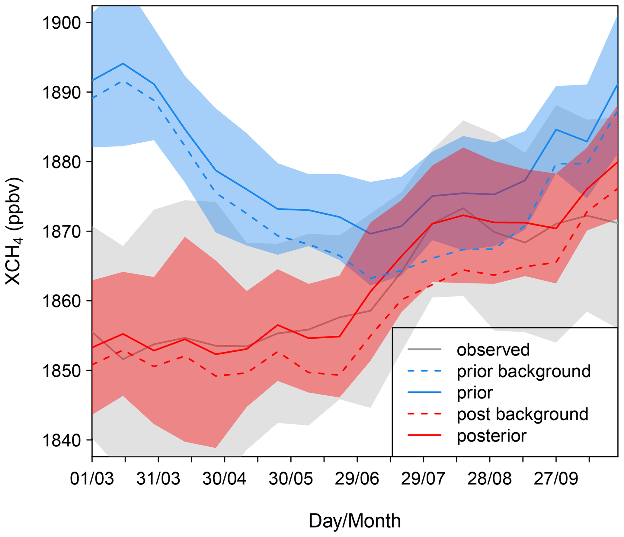
Figure 4 Area-weighted mean XCH₄ for 2-weekly intervals integrated over the domain for the inversion using EGG4 for the boundary conditions. The shading shows the area-weighted standard deviation of XCH₄ in each 2-weekly interval over the domain.

Figure 4 shows the area-weighted mean XCH₄ for the domain for 2-weekly intervals from March to October. The prior modelled XCH₄ follows the prior background estimate, which is driven by variations in the boundary conditions (based on EGG4) and differs considerably from the variation in the observed XCH₄. After optimization, the modelled XCH₄ more closely follows the observations, which is largely due to the improvement to the background estimate. Both the prior and posterior modelled XCH₄ remain close to their respective backgrounds until late April, when fluxes in the domain start to increase and, thus, have a more significant impact on XCH₄ and return towards their background estimate after September.

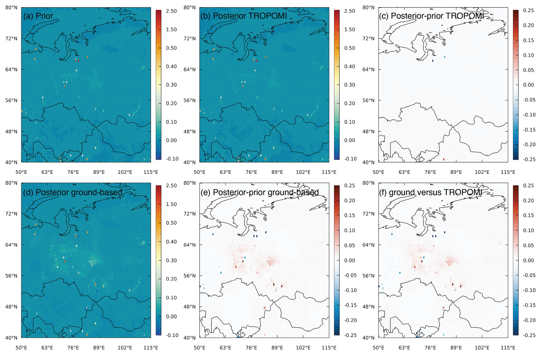
Figure 5 Mean CH₄ flux and flux increments (in g m⁻² d⁻¹) from the inversions for (a) prior fluxes, (b) the posterior flux using TROPOMI, (c) the posterior minus prior flux increments using TROPOMI, (d) the posterior flux using ground-based observations, (e) the posterior minus prior flux increments using ground-based observations, and (f) the difference in posterior fluxes using ground-based observations versus TROPOMI.

3.2.3 Posterior fluxes and uncertainty reduction using TROPOMI

Figure 5 shows the mean posterior fluxes estimated from the inversion using TROPOMI observations as well as the posterior minus prior differences (flux increments). Overall, the posterior fluxes remain very close to those of the prior, and the total mean posterior source over the domain for March to October is 30.3±22.7 Tg yr⁻¹ compared to the prior estimate of 31.0±24.5 Tg yr⁻¹. The seasonal cycle also remained close to the prior estimate, with a maximum in late July to early August (Fig. 6). The inversion did, however, reduce emissions for a few hotspots in northwestern Siberia, in grid cells with important oil and gas sources, and increase emissions for a few hotspots in northern China, again in grid cells with important oil and gas sources.

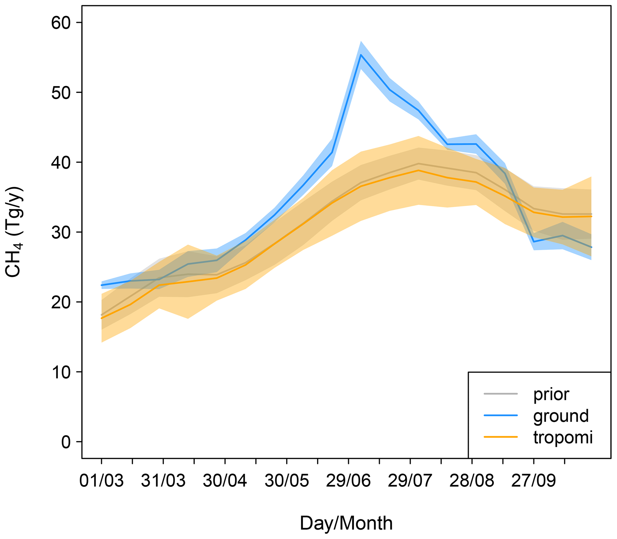
Figure 6 Total CH₄ source for the domain shown on a 2-weekly timescale for the prior estimate and for the posterior estimates from the TROPOMI and ground-based observation inversions.

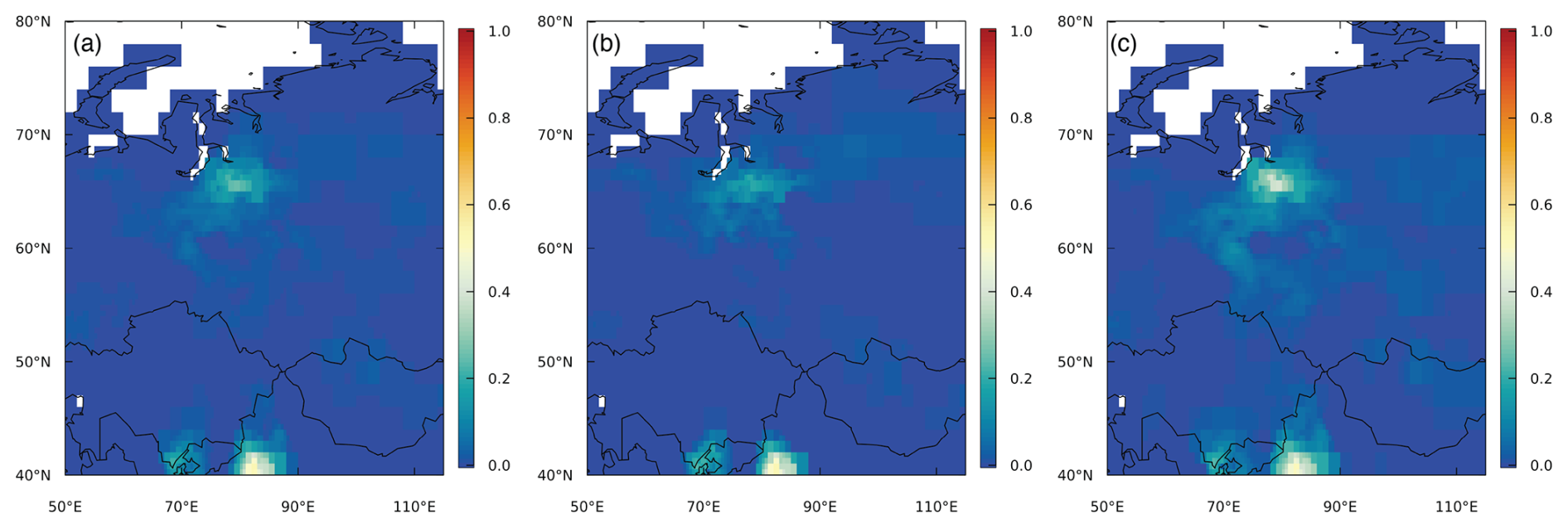
Figure 7 Uncertainty reduction for the inversion using the TROPOMI (a) mean of March–October, (b) mean of March–May, and (c) mean of June–August.

It must be noted, however, that the uncertainty reduction on the fluxes (calculated as 1 minus the ratio of the posterior to prior flux uncertainty) is quite small and mainly limited to the areas of the West Siberian Plain and to the southern part of the domain, where it reaches 20 %–50 % (Fig. 7). This is similar to the results of Tsuruta et al. (2023), who likewise found a limited uncertainty reduction for the high northern latitudes using TROPOMI and little difference between the prior and posterior fluxes for their region of Eurasia (which included Fennoscandia). This is partly due to the poor observational coverage over Siberia, where (even outside of the winter season) the number of observations is still limited (especially >50° N) and can be due to frequent cloud cover (Gao et al., 2023). (The low uncertainty reduction is discussed further in Sect. 3.2.4.) The pattern of uncertainty reduction in our study is persistent for all months and is largely determined by the distribution of observations and of the prior flux uncertainty. The more southern part of the domain is better covered by observations, especially over Kazakhstan and northern China, while the prior flux uncertainties followed the distribution of the prior fluxes with larger uncertainties in the area of the West Siberian Plain and for grid cells with hotspot emissions (see Fig. S10).

3.2.4 Comparison with ground-based data inversions

Figure 5d and e show the posterior fluxes and flux increments, respectively, from the inversion with ground-based observations. The mean posterior fluxes show large emissions over the West Siberian Plain, and generally higher emissions than in the prior estimate. They also indicate that some of the hotspot emission sources in northwestern Siberia are too large in the prior, which is consistent with the result of the inversion using TROPOMI. Moreover, the posterior fluxes indicate larger emissions for a few hotspots in southern Siberia coinciding with grid cells where there are coal mines. The mean posterior source over the domain from March to October is 34.6±10.2 Tg yr⁻¹. The difference between the posterior fluxes from the inversion using ground-based observations versus that using TROPOMI (Fig. 5f) follows a very similar pattern to the posterior minus prior flux increments (Fig. 5d), as expected, because the posterior fluxes from the inversion using TROPOMI are very close to the prior.

The ground-based observation inversion indicates an earlier and more intense summer maximum compared to the prior estimate and to the estimate from the TROPOMI-based inversion (Fig. 6). In the ground-based inversion, the maximum occurs in early July, versus late July to early August in the prior, and it reaches a maximum of 51.8 Tg yr⁻¹ for the mean of July versus 37.8 Tg yr⁻¹ in the prior.

Moreover, the inversion using ground-based observations is better constrained than that using TROPOMI, and there are uncertainty reductions of up to 50 % over a significant part of western Siberia, corresponding to where the continuous measurement sites are located, although some gaps remain (Fig. 8). On the other hand, the southern and eastern parts of the domain are not well constrained.

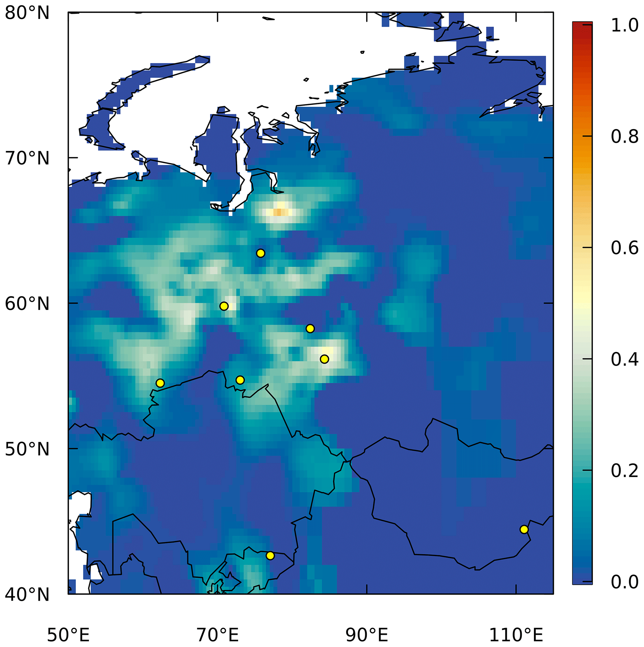
Figure 8 Uncertainty reduction for the inversion using ground-based observations. The observation sites are indicated by the yellow circles.

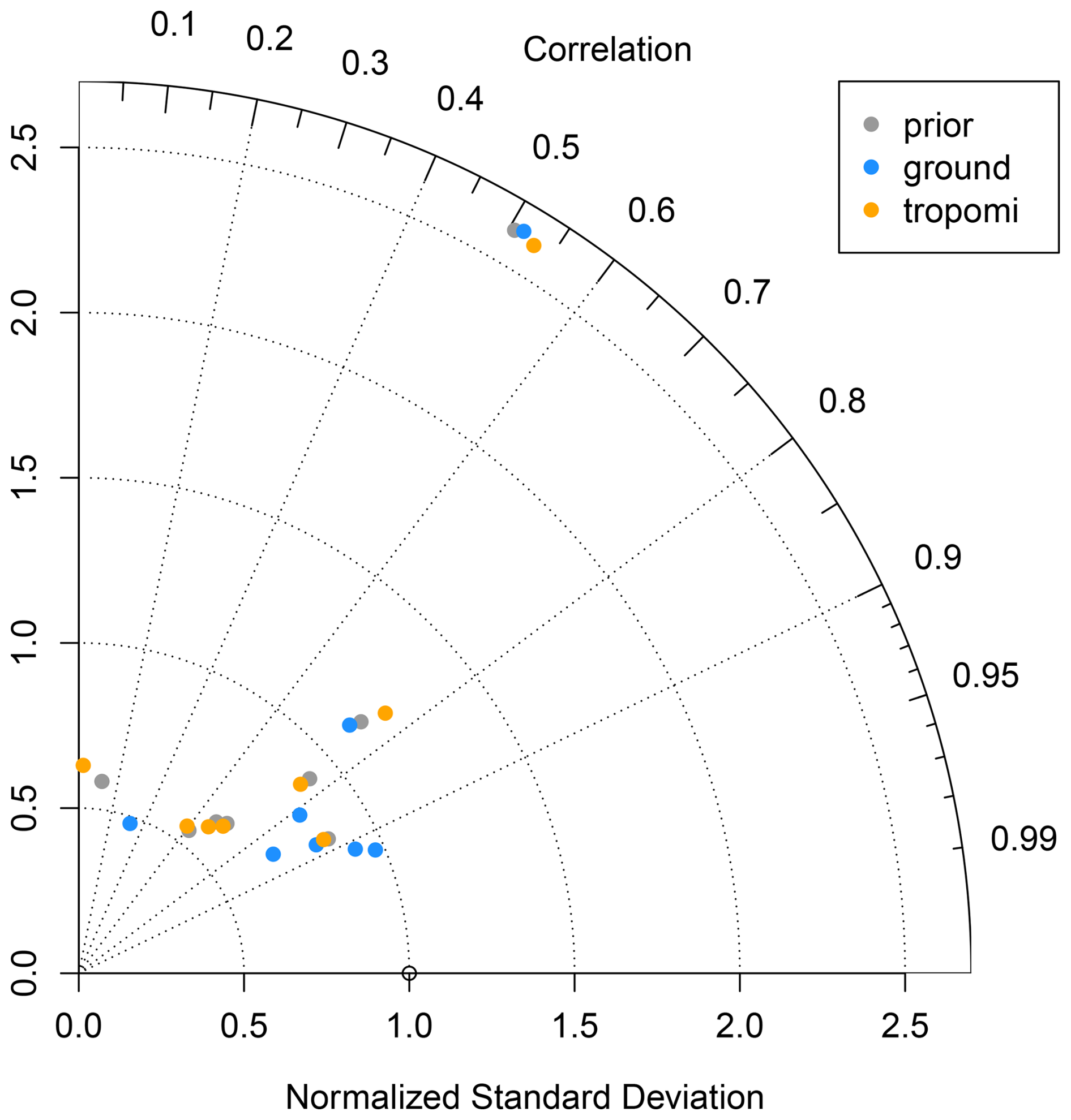
Figure 9 Taylor diagram for the comparison of modelled versus observed CH₄ mixing ratios at ground-based sites. The angle gives the Pearson correlation, and the x axis gives the normalized standard deviation for the comparison. Each point represents a site, and the colour of the point indicates the modelled data used (prior: using the prior fluxes; ground: using the posterior fluxes from the inversion with ground-based observations; and tropomi: using posterior fluxes from the inversion with TROPOMI observations). All model simulations used optimized boundary conditions to compare differences solely due to the fluxes used.

As a further check on the inversion using TROPOMI observations, we compared the mixing ratios modelled using the prior fluxes, the posterior fluxes from the ground-based inversion, and the posterior fluxes from the TROPOMI inversion against observations at all ground-based sites (Fig. 9). In this comparison, the optimized boundary conditions were used to show only the differences due to the fluxes. Overall, there is an improvement in the fit to the observations using the posterior fluxes from the ground-based inversion compared to the prior fluxes, as would be expected, because these observations were used in the inversion. The RMSE over all observations was reduced from 37 ppb a priori to 24 ppb a posteriori. However, employing the posterior fluxes from the inversion using TROPOMI observations did not lead to an improvement (nor a deterioration) in the fit to the observations, which is simply because, in this case, the posterior fluxes remained very close to the prior.

The reason for the lower uncertainty reduction (and smaller flux increments) using TROPOMI versus ground-based observations is essentially twofold. First, the TROPOMI column average observations have larger uncertainties compared to the ground-based observations (in this study, the median uncertainty used for ground-based observations was 12 ppb versus 16 ppb for TROPOMI) and the model–observation errors are weighted by the inverse of the square of the observation uncertainties (see Eq. 15). Second, as satellite observations are of the total atmospheric column, the air masses in the columns can have more diverse source regions, resulting in column SRRs that are more spread out compared to those of point observations. This tends to lead to smaller deviations over the background for the satellite observations compared to the point observations, and, as the cost function depends on the square of the model–observation differences, a few large differences have more influence than a larger number of small differences. Thus, to compensate for the weaker constraint of each individual retrieval on the fluxes, many more retrievals are needed to achieve a similar constraint as provided by the point observations. Although this applies for any region, this is more notable at higher latitudes, where there are generally fewer observations compared to mid-latitudes and where the background uncertainty is larger, meaning that even greater departures in the modelled mixing ratios from the background mixing ratio would be needed to constrain the fluxes.

4 Summary and conclusions

We have developed an efficient method to model total column observations, such as those from satellites, for Lagrangian particle dispersion models (LPDMs) and, furthermore, to compute Jacobian matrices describing the relationship between fluxes and the change in the column average mixing ratio, as needed in inverse modelling. This method means that the computations are, in principle, no more costly than those for point observations. The development will enable a more accurate representation of satellite observations (especially high-resolution ones) via the use of LPDMs and, thus, help to improve the accuracy of emission estimates obtained via atmospheric inversions.

As LPDM backward calculations are still needed for each observation, the computational cost is a limiting factor with respect to using this method on a global scale for satellites providing a very large number of retrievals, e.g. TROPOMI which provides ∼100 000 retrievals globally each day. However, this limitation can be overcome using super-observations, which are averages of retrievals and reduce the number of calculations required. On the other hand, our method using an LPDM is well suited for regional inversion studies, especially with observations from flux mapping satellites with a relatively high resolution, such as the TROPOMI XCH₄ product with a resolution of 5.5 × 7 km, MethaneSAT with a resolution of 0.1 × 0.4 km, the recently launched GOSAT-GW with a resolution of 1 × 1 to 3 × 3 km in Focus mode, and the future mission CO2M with a resolution of 2 × 2 km.

We presented a case study using the methodology to estimate CH₄ fluxes over Siberia using WFMD retrievals of XCH₄ from the TROPOMI instrument. We found that, for this northern region, the boundary conditions have a strong influence on the modelled column mixing ratios; however, by optimizing the boundary conditions, any bias in the boundary conditions does not contribute to a bias in the posterior fluxes. Moreover, we compared the inversion with TROPOMI to one using ground-based observations. The ground-based observations provide a stronger constraint on the fluxes and greater uncertainty reduction compared to TROPOMI for this northern region. Although the posterior fluxes obtained using TROPOMI remained close to the prior, there were some consistent results with those obtained using ground-based observations, namely, a decrease in hotspot emissions in northern Siberia and an increase in a hotspot emission in northern China compared to the prior emissions.

Based on these results, the caveats of using satellite retrievals in regional inversions at high latitudes are as follows: (1) the strong dependence of the modelled column mixing ratios on the boundary conditions and, hence, the need to set large uncertainties for the optimization of the boundary conditions, which has the effect of reducing the constraint of the observed column average mixing ratios on the fluxes; (2) the limited observational constraint of the column average mixing ratios on surface fluxes in Siberia and, hence, low uncertainty reduction from inversions.