Global atmospheric inversion of the anthropogenic NH₃ emissions over 2019–2022 using the LMDZ-INCA chemistry transport model and the IASI NH₃ observations

Ammonia (NH₃) emissions have been on a continuous rise due to extensive fertilizer usage in agriculture and increasing production of manure and livestock. However, the current global-to-national NH₃ emission inventories exhibit large uncertainties. We provide atmospheric inversion estimates of the global NH₃ emissions over 2019–2022 at 1.27° × 2.5° horizontal and daily (at 10 d scale) resolution. We use IASI-ANNI-NH3-v4 satellite observations, simulations of NH₃ concentrations with the chemistry transport model LMDZ-INCA, and the finite difference mass-balance approach for inversions of global NH₃ emissions. We take advantage of the averaging kernels provided in the IASI-ANNI-NH3-v4 dataset by applying them consistently to the LMDZ-INCA NH₃ simulations for comparison to the observations and then to invert emissions. The average global anthropogenic NH₃ emissions over 2019–2022 are estimated as ∼97 (94–100) Tg yr⁻¹, which is ∼61 % (∼55 %–65 %) higher than the prior Community Emissions Data System (CEDS) inventory's anthropogenic NH₃ emissions and significantly higher than two other global inventories: CAMS's anthropogenic NH₃ emissions (by a factor of ∼1.8) and the Calculation of AMmonia Emissions in ORCHIDEE (CAMEO) agricultural and natural soil NH₃ emissions (by ∼1.4 times). The global and regional budgets are mostly within the range of other inversion estimates. The analysis provides confidence in their seasonal variability and continental- to regional-scale budgets. Our analysis shows a rise in NH₃ emissions by ∼5 % to ∼37 % during the COVID-19 lockdowns in 2020 over different regions compared to the same-period emissions in 2019. However, this rise is probably due to a decrease in atmospheric NH₃ sinks due to the decline in NO_x and SO₂ emissions during the lockdowns.

1 Introduction

Ammonia (NH₃) plays a critical role in both atmospheric chemistry and the ecosystem's nitrogen and carbon cycling, with significant implications for air quality and human health, climate change, and agriculture. Ammonia in the Earth's atmosphere originates from both natural and anthropogenic sources, with the latter dominating emissions from the former. The agricultural sector is the largest source of NH₃ emissions, contributing more than 81 % of the total global NH₃ emissions (Van Damme et al., 2021; Wyer et al., 2022), and other anthropogenic sources of NH₃ mainly stem from domestic, vehicular, waste water treatment, and industrial activities (Behera et al., 2013a; Sutton et al., 2013). Global future NH₃ emissions in 2100 are projected to increase by 30 % to 50 % compared to present-day levels, depending on the different Shared Socioeconomic Pathways scenarios (Beaudor et al., 2025). Precise information on the NH₃ sources and quantitative attribution of emissions to these sources and atmospheric NH₃ concentration observations are essential in evaluating the impacts of NH₃ on ecosystems, climate, air quality, and human health and in formulating effective mitigation measures (Zhu et al., 2015). Timely estimates of global anthropogenic NH₃ emissions are needed to formulate effective control strategies to reduce such emissions activities (Behera et al., 2013).

Bottom-up NH₃ emission inventories provide data on NH₃ sources and their emissions (Beaudor et al., 2023; Bouwman et al., 1997; Vira et al., 2020), enabling their integration into atmospheric chemistry transport and climate models to simulate atmospheric ammonia concentrations and making it possible to assess the impacts of NH₃ emissions. However, significant uncertainties are inherent in bottom-up NH₃ emission inventories across spatiotemporal scales (Behera et al., 2013; Luo et al., 2022; Sutton et al., 2013), stemming from the constraints of limited NH₃ emission activity data and emission factors, high uncertainty of agriculture statistics, and a lack of recent information (Chen et al., 2021; Crippa et al., 2018; Xu et al., 2019). In situ measurements are essential for accurately developing NH₃ emission inventories and for the inversion of NH₃ emissions, as well as for evaluating these emissions. However, the scarcity of in situ NH₃ measurements worldwide contributed to significant uncertainties in NH₃ emissions and in our understanding of NH₃ sources and their distributions (Zhu et al., 2015). Advancements in satellite measurements of columnar NH₃ abundance in the atmosphere in the past decades provide high-spatiotemporal-resolution column concentration data, and inversion methods are progressively enhancing our ability to derive NH₃ emissions. For the atmospheric inverse modeling of the NH₃ emissions, satellite observations offer valuable data density and coverage, thus mitigating some of the limitations of the use of in situ NH₃ measurements, enabling a more comprehensive assessment of NH₃ emissions. The recent NH₃ emission estimates based on satellite observations exhibit significant differences at both regional and global scales when compared to those reported by the bottom-up inventories (Cao et al., 2020; Chen et al., 2021; Van Damme et al., 2018; Luo et al., 2022; Evangeliou et al., 2021; Dammers et al., 2022). However, the satellite data also have some limitations, often lacking clear signals from the emissions outside the strongly polluted regions, bearing potential errors due to interference from other atmospheric constituents and the complexity of their validation and calibration, and being sensitive to cloud cover, providing incomplete coverage in certain regions in the presence of clouds.

Currently, satellite NH₃ observations are available from instruments such as the Atmospheric Infrared Sounder (AIRS) on the NASA EOS Aqua satellite (Warner et al., 2016), the Aura Tropospheric Emission Spectrometer (TES) on board the EOS Aura satellite (Beer et al., 2008), three of the Infrared Atmospheric Sounding Interferometer (IASI) series of instruments on the MetOp (Meteorological Operational satellite program) satellites (Clarisse et al., 2009; Van Damme et al., 2021), the Thermal And Near-infrared Spectrometer for Observation–Fourier Transform Spectrometer (TANSO-FTS) on board the Greenhouse Gases Observing Satellite (GOSAT) (Someya et al., 2020), and the three Cross-track Infrared Sounder (CrIS) instruments on board the Suomi National Polar-orbiting Partnership (Suomi-NPP) satellites (Shephard et al., 2020). These datasets vary in their data record lengths, spatial coverage, and retrieval approaches. The NH₃ observations derived from the IASI and CrIS measurements, which have similar instrumental characteristics but employ different retrieval approaches, are the most commonly used satellite data for constraining NH₃ emission estimates. The IASI NH₃ product is a widely used dataset, as it provides continuous, long-term sampling commencing from 2007, with twice-daily coverage across the globe. Except for its first version, subsequent versions of the IASI NH₃ data products are based on the Artificial Neural Network for IASI (ANNI) approach for the retrieval of NH₃ total columns (Van Damme et al., 2017, 2021; Whitburn et al., 2016). However, the absence of the vertical averaging kernel (AK) in the IASI ANNI NH₃ previous products hindered their utility for comprehensive comparisons to the atmospheric chemistry transport model and its suitability for assimilation in atmospheric inversion processes for NH₃ emission estimations. The AK is proportional to the measurement vertical sensitivity profile and also describes the vertical structure of the impact of a priori information on the retrieval of NH₃ columns. When comparing a chemistry transport model against the satellite column retrievals, e.g., in satellite data assimilation processes, the application of the AK should remove the influence of errors resulting from the a priori (or an assumed) atmospheric NH₃ vertical profile used in the retrievals in the model–satellite comparison (Eskes and Boersma, 2003). Using synthetic satellite column observations of another short-lived species (NO₂), Cooper et al. (2020) examined the impact of differences between the modeled and a priori atmospheric vertical NO₂ profiles on the inversion of NO_x emission estimates and found that discrepancies led to an up to 30 % increase in root mean square errors for realistic conditions over polluted regions, with inverted emission errors rising as the difference between simulated and a priori profiles increases. The application of AK enables the model-retrieval comparison to be independent of the a priori profile (Cooper et al., 2020; Douros et al., 2023). Recently, Clarisse et al. (2023) presented a new version 4 of the ANNI retrieval framework including, for the first time, vertical AK in the IASI NH₃ data product. In this study, we use this new version 4 of the IASI ANNI NH₃ dataset for comparison to the global chemistry transport model simulations and for the atmospheric inversion of the global NH₃ emissions.

In recent years, numerous studies have used satellite observations, mostly IASI and CrIS, to estimate NH₃ emissions over specific regions (Cao et al., 2020, 2022; Chen et al., 2021; Ding et al., 2024; Fortems-Cheiney et al., 2020; Tichý et al., 2023; Xia et al., 2025) or across the globe (Dammers et al., 2022; Evangeliou et al., 2021; Luo et al., 2022). Some recent regional-scale inversion studies over the USA (Cao et al., 2020; Chen et al., 2021), China (Jin et al., 2023; Momeni et al., 2024), UK (Marais et al., 2021), and Europe (Cao et al., 2022; Ding et al., 2024; van der Graaf et al., 2022) show approximately 20 %–100 % differences between the inversion-based and the bottom-up NH₃ emissions. The NH₃ inversion problem raises challenges and requires a high spatial resolution of the emissions because the NH₃ emissions are highly localized due to the short lifetime of a few hours to a day of ammonia in the atmosphere. The impact of the atmospheric chemistry challenges the linearization underlying the traditional inversion approaches or the use of relatively simple models of the atmospheric chemistry and transport. The conventional variational or Kalman filter approaches, which are among the most sophisticated ones, have been used for regional-scale inversions (Cao et al., 2020, 2022; Ding et al., 2024; Jin et al., 2023). However, covering the globe at a suitable spatial resolution represents an inversion problem whose dimensions make the application of such approaches very demanding in terms of computational cost. That is probably why, compared to regional studies, global inversions of NH₃ emissions based on satellite observations are relatively scarce (Van Damme et al., 2018; Dammers et al., 2022; Evangeliou et al., 2021; Luo et al., 2022). Studies such as Van Damme et al. (2018) and Dammers et al. (2019) covered emissions worldwide but focused on the detection and estimation of NH₃ large point sources or hotspot areas. Using high-resolution maps of atmospheric ammonia from IASI, Van Damme et al. (2018) detected 248 NH₃ hotspot locations and large source regions across the globe and reported that the satellite-data-constrained NH₃ emissions for the source regions vary within a factor of 3 from the corresponding estimates extracted from the Emissions Database for Global Atmospheric Research (EDGAR) emission inventory. However, the emissions from these detected large NH₃ point sources or source regions account for only a small fraction of the overall global NH₃ emissions budget (Dammers et al., 2019). For instance, the cumulative NH₃ emissions from the 249 point sources identified by Dammers et al. (2019) contributed to merely 5 % of the total global NH₃ emissions in the Hemispheric Transport Atmospheric Pollution version 2 (HTAPv2) inventory.

Only very few global-scale inversion studies provided more comprehensive time series of full NH₃ emission maps using computationally intensive inversion frameworks. Recently, Dammers et al. (2022) derived global NH₃ emission maps at a high spatial resolution (0.2° × 0.2°) based on a multi-source Gaussian plume method using CrIS observations, discarding any chemistry or aerosol mechanism associated with the short-lived species NH₃ in the multi-source Gaussian plume method. They showed that satellite-based total NH₃ emissions over the globe are ∼1.8 times higher than those reported in previously identified anthropogenic NH₃ source locations in the CAMS-GLOB-ANT v4.2 global anthropogenic NH₃ emission inventory, and the total estimates rise to ∼4 times greater when newly detected anthropogenic and natural sources are taken into account. However, this approach also introduces uncertainties in the estimates due to the assumption of a globally constant atmospheric lifetime for NH₃, which is a limiting factor because chemical loss and deposition are highly variable processes that can change the lifetime drastically (Van Damme et al., 2018), and uncertainties in plume spread, wind speed, and wind direction when fitting a multi-source Gaussian plume model to the observations.

In two recent studies of the global inversion of NH₃ emissions using previous versions of the IASI ANNI NH₃ data products, Evangeliou et al. (2021) and Luo et al. (2022) estimated long-term monthly global NH₃ emissions over a decade starting from 2008 and reported their estimates to be higher than those in the bottom-up inventories. However, significance differences were observed between these two NH₃ emission estimates. In both studies, inversions rely on the NH₃ lifetime, diagnosed differently from the simulations of different global chemistry transport models (CTMs), and the modeled NH₃ total columns. Evangeliou et al. (2021) applied a basic mass-balance inversion approach to estimate monthly NH₃ emissions in each grid cell as a ratio of the observed total NH₃ column from IASI and the lifetime of NH₃ computed from CTM simulations. Using a previous version of IASI NH₃ observations, Luo et al. (2022) modified the basic mass-balance approach used in Evangeliou et al. (2021) by updating the prior NH₃ emissions with an additive correction term. This correction is proportional to the difference between the observed and modeled NH₃ columns and inversely proportional to the NH₃ lifetime estimated by accounting for the deposition fluxes of the whole NH_x (NH₃+ NH${}_{\mathrm{4}}^{+}$) family instead of using only the NH₃ losses. However, estimating the lifetime of NH₃ in the atmosphere is more complex due to the impact of transport mechanisms, loss of atmospheric NH₃ by the formation of ammonium sulfate or ammonium nitrate particles (Cao et al., 2020), and non-linearities in NH₃-related chemistry affecting deposition and concentration. Changes in NH₃ concentrations due to emission affect its lifetime through its interaction with other trace chemical species like SO₂, NO_x, HCl, and HONO (Behera et al., 2013), and the basic mass-balance approaches in Evangeliou et al. (2021) and Luo et al. (2022) do not consider the impact of NH₃ emission changes in their estimation of NH₃ lifetime in atmospheric inversions, which may affect the accuracy of emission estimates.

Variations of the mass-balance inversion methodology, such as the finite difference mass-balance (FDMB) approach (Cooper et al., 2017; Lamsal et al., 2011), have been proposed for atmospheric inversion of emissions of short-lived species, which aims to reduce errors in basic mass-balance methods due to non-linear sensitivity between species emissions and ambient concentrations. The FDMB inversion approach is computationally efficient for the global-scale inversions at coarse resolutions, and it has been widely used for estimating anthropogenic surface emissions of short-lived species like NO_x and SO₂ at global and regional scales (Cooper et al., 2017; Lamsal et al., 2011). It derives the fluxes by scaling a priori emission estimates, usually derived from bottom-up inventories. This scaling is derived from the computation of the local sensitivity of concentrations to local emission changes from simulations with a CTM and from the relative differences between observations and the modeled columns. Only a few studies have investigated the FDMB approach for NH₃ emission inversion at regional scales: Momeni et al. (2024) and Li et al. (2019). They applied the iterative FDMB approach to constrain the NH₃ emissions of East Asia with CrIS and North America with IASI satellite observations. In this study, we investigate the use of the FDMB approach at the global scale to derive maps of the NH₃ emissions at a relatively high temporal resolution worldwide. While earlier global-scale inversion studies by Luo et al. (2022) and Evangeliou et al. (2021) derived NH₃ emission estimates at the 1-month scale, we aim to provide daily estimates at the 10 d scale (deriving 10 d running average). The FDMB inversion approach involves a chemistry transport model for simulations of NH₃ concentrations. We use the global chemistry–aerosols transport model LMDZ-INCA (Hauglustaine et al., 2004, 2014) for global NH₃ concentration simulations. Our LMDZ-INCA model configuration has a relatively high spatial resolution of 1.27° × 2.5° (latitude × longitude) horizontally and 79 vertical levels. The absence of the averaging kernel in previous versions of the IASI ANNI NH₃ data products used in the previous inversion studies prevented utilization of this information to integrate the modeled NH₃ profile consistently with the IASI NH₃ retrievals. This limitation may have impacted the final NH₃ emission estimates. In this study, we take advantage of the availability of AKs in version 4 of the IASI NH₃ product for suitable assimilation of such data into a global inversion framework relying on a CTM. The application of AK in our global atmospheric inversion of NH₃ emissions with the new version 4 of the IASI NH₃ retrievals is one of the main features in this study.

Here, we estimate global daily (as a 10 d running average) anthropogenic NH₃ emissions over the land at 1.27° × 2.5° horizontal resolution across a period of 4 years from 2019 to 2022 using the new version 4 of the IASI ANNI NH₃ data product and the FDMB inversion approach (Cooper et al., 2017; Lamsal et al., 2011). We first compare the LMDZ-INCA model global NH₃ simulations against the IASI NH₃ observations to assess our model's performance and its suitability for global inversions of NH₃ emissions. In both model–satellite comparisons and inversions, we take advantage of averaging kernels provided in version 4 of the IASI ANNI NH₃ data product to remove the impact of the vertical NH₃ profile assumption in the retrievals. We present and discuss the results of our model comparison analysis with the IASI NH₃ observations and the global inversions of the NH₃ emissions at both global and regional scales, considering temporal scales ranging from daily (10 d scale) to monthly, seasonal, and annual. We evaluate our inversion approach and emissions estimates by conducting LMDZ-INCA simulations using the optimized NH₃ emissions and comparing the model results with the IASI NH₃ observations. Finally, we compare our estimated global NH₃ emissions with independent global bottom-up inventories and other estimated NH₃ emissions over the globe and over the selected regions. The structure of the paper is as follows. Section 2 describes the new version 4 of the IASI NH₃ observations, the chemistry transport model and its setup for global NH₃ concentration simulations, our strategy to compare model NH₃ simulations with the satellite observations, and the FDMB inversion approach used for global daily NH₃ emission estimations. Section 3 presents the results, followed by a discussion of those results and the limitations of the study in Sect. 4. Key conclusions of this study are provided in Sect. 5.

2 Material and methods

2.1 IASI NH₃ version 4 observations

IASI is an infrared Fourier transform spectrometer on board the sun-synchronous polar-orbiting MetOp-A/B/C satellites, which were respectively launched in 2006, 2012, and 2018 (Clerbaux et al., 2009). IASI has a cross-track scanning swath width of ∼2200 km, with a pixel size of ∼12 km in diameter at nadir. Each instrument on board one of the sun-synchronous satellites covers almost all locations over the globe twice a day, once at daytime and once at nighttime, with overpasses around 09:30 and 21:30 local solar time (LST), respectively. The vertical sensitivity of the IASI NH₃ measurements, mainly in the boundary layer where NH₃ is predominantly confined, varies as a function of the thermal contrast between the surface and the atmospheric layers (Clarisse et al., 2010; Di Gioacchino et al., 2024). The NH₃ total column observations from the IASI measurements in the first version were retrieved using the so-called hyperspectral range index (HRI) in an extended spectral range (800–1200 cm⁻¹) and using look-up tables (LUTs) built from forward radiative transfer model simulations (Van Damme et al., 2014). In the subsequent versions, an artificial neural network for the IASI (ANNI) retrieval approach was then developed and used for retrievals of IASI NH₃ total columns (Van Damme et al., 2017, 2021; Whitburn et al., 2016). The ANNI NH₃ retrieval approach uses an assumed Gaussian-shaped vertical profile of the NH₃ volume mixing ratio (the “prior” profile), which is modeled as a function of the altitude above the ground or ocean surface, the peak concentration altitude, and the width of the profile of significant NH₃ concentrations. The peak altitude over land is set at the ground surface with a width equal to the boundary layer height (Clarisse et al., 2023), as the NH₃ emission is generally higher near the surface and NH₃-related chemistry and dispersion cause the concentration to decrease with altitude. Over the ocean, it is set to 1.4 km with a width of 0.9 km (Clarisse et al., 2023). In this study, we use daily NH₃ total columns from a recently released version 4 (ANNI-NH3-v4) of the IASI ANNI retrievals of NH₃ (Clarisse et al., 2023). The most important feature of this new ANNI-NH3-v4 data product is the introduction of the column averaging kernel (AK). The vertical AK is essential for comparison of chemistry transport model simulations against the satellite NH₃ retrievals, which can be used to remove the effect of the prior vertical NH₃ profiles used in the retrievals of the IASI NH₃ total columns in the model–satellite comparison. Note that the NH₃ distribution from IASI-ANNI-v4 is very similar to the ones with the previous version 3, although the values are about 15 %–20 % larger due to the improved setup of the HRI (Clarisse et al., 2023). Furthermore, the ANNI-NH3-v4 data product provides a more accurate characterization of the measurement uncertainty, along with several other changes, resulting in the improved temporal consistency of the IASI NH₃ dataset spanning from 2007 onwards (Clarisse et al., 2023).

We use daily IASI-NH3-v4 NH₃ global observations over land from the MetOp-B satellite from 2019 to 2022. We select only the NH₃ observations from the morning overpass (around 09:30 LST) because of the better precision of morning observations, as IASI is more sensitive at this time of day to the atmospheric boundary layer, where the signature of the surface emissions is higher, owing to more favorable thermal conditions. We use high-quality IASI NH₃ observations only with the cloud coverage lower than and equal to 10 % (Clarisse et al., 2023). We apply pre- and post-retrieval filters that accompany the dataset. The application of these filters removes respectively the observations corresponding to erroneous L1 processing of the spectra or excess cloud coverage and the observations corresponding to measurements with limited or no sensitivity to the measured quantity and retrievals satisfying certain threshold conditions (Clarisse et al., 2023).

2.2 LMDZ-INCA global chemistry transport model and simulations

We use the global climate–aerosol–chemistry transport model LMDZ-INCA to simulate the global NH₃ concentrations, along with a state-of-the art gas phase tropospheric chemistry scheme as well as aerosols including sulfate, nitrate, black carbon (BC), particulate organic matter (POM), dust, and sea salt. LMDZ-INCA is a coupled model based on an atmospheric general circulation model (GCM) LMDZ V6 (Laboratoire de Météorologie Dynamique) (Boucher et al., 2020; Hourdin et al., 2020), a chemistry and aerosols model INCA V6 (INteraction with Chemistry and Aerosol) (Hauglustaine et al., 2004, 2014), and a global land surface dynamical vegetation model ORCHIDEE (ORganizing Carbon and Hydrology In Dynamic Ecosystems) (Krinner et al., 2005). The model uses a monotonic, finite-volume, second-order parameterization to calculate large-scale advection of water vapor, liquid and solid water, and tracers (Boucher et al., 2020). The model uses the “New Physics” (NP) version of the physical parameterizations, which includes a turbulent scheme based on the prognostic equation for the turbulent kinetic energy (Yamada, 1983), the “Thermal Plume Model” for the convective boundary layer (Rio and Hourdin, 2008), a parameterization for cold pools and wakes resulting from convective rainfall evaporation (Grandpeix and Lafore, 2010), and Emanuel's deep convection parameterization scheme (Emanuel, 1991). LMDZ-INCA interactively accounts for the emissions, transport (resolved and subgrid scales), and deposition (both dry and wet) of chemical species and aerosol, and it incorporates a full chemical scheme for the NH₃ cycle and nitrate particle formation (Hauglustaine et al., 2014).

The LMDZ-INCA model configuration used in this study has a horizontal resolution of 1.27° latitude ×2.5° longitude with 79 hybrid σ-pressure levels within a terrain following vertical coordinate stretches up to 80 km. We conducted LMDZ-INCA spin-up simulations from 2010 to 2018 and then reference simulations for a period of 4 years from 2019 to 2022, which we used for the model comparison with the IASI NH₃ observations and for the global NH₃ emission inversions. The simulations were driven by nudging the GCM winds with a 3.6 h relaxation time to the 6-hourly ECMWF Reanalysis v5 (ERA5) data, regridded onto the LMDZ-INCA model grid. In the LMDZ-INCA simulations, we used the monthly global anthropogenic emission of the chemical species and gases, including NH₃, from the open-source Community Emissions Data System (CEDS) global bottom-up gridded inventories (McDuffie et al., 2020), with an initial horizontal resolution of 0.5° × 0.5°, interpolated onto the model horizontal grid. We used conservative regridding by ensuring that the total mass (e.g., emissions) was preserved during the interpolation. The CEDS global emission inventories provide emissions of NH₃, NO_x, SO₂, NMVOCs, CO, OC, and BC from 11 anthropogenic sectors, including agriculture, energy, on-road and non-road transportation, residential, commercial, waste solvents, international shipping, and others (McDuffie et al., 2020). The CEDS inventory also includes emissions of NO and NH₃ from agricultural soils with both synthetic and manure fertilizers. Because CEDS anthropogenic emissions are available only up to 2019, the CEDS emission fluxes for the post-2019 years were developed based on the combination of the CEDS emissions in 2019 with the carbon emission growth rate from 2019 to the target year. The data on the emissions growth rate were derived from the Carbon Monitor dataset (https://carbonmonitor.org/, last access: 1 August 2024) and calculated by source sector, by month, and by country. This approach to extrapolate emission fluxes based on CO₂ data has been commonly applied to various species, particularly those associated with fossil fuel emissions. This has led to noticeable variations in emissions of species like SO₂ and NO_x, which have been simultaneously used in the LMDZ-INCA simulations with the full chemical scheme for sulfate and nitrate particle formation (Fig. S1 in the Supplement). However, as extrapolation calculations are conducted for each source sector separately and NH₃ emissions mostly come from agricultural activities, which do not emit CO₂ directly, applying this approach to extrapolate NH₃ emissions for the post-2019 years resulted in almost invariant NH₃ emissions after 2019 (Fig. S1). While this approach may seem simplistic for NH₃ fluxes, it was used in this study to construct the spatial distribution of prior emissions, as we expect satellite data to drive year-to-year variations in the final inversion results. Because the anthropogenic emissions are derived from the CEDS inventory at a monthly resolution, they are uniformly distributed in time at the hourly resolution in the input to the LMDZ-INCA simulations, without incorporating diurnal cycles. We used fire emissions from the Global Fire Emissions Database (GFED4) (van der Werf et al., 2017) and biogenic volatile organic compound (VOC) emissions calculated from the ORCHIDEE vegetation model (Messina et al., 2016). Emission fluxes from anthropogenic and natural sources were prescribed to the model as monthly forcing files for different species. We sampled the simulated NH₃ concentration at an hourly frequency over a 4-year period from 2019 to 2022. We used these hourly LMDZ-INCA model-simulated NH₃ data for our analysis and inversions with IASI NH₃ observations from the morning overpass.

2.3 Model and satellite comparison approach

The retrievals of NH₃ total column observations, Ω_obs, where “obs” stands for the “observed” IASI NH₃ total columns in the IASI-ANNI-NH3-v4 data product, are implicitly dependent on assumed (prior) Gaussian-shaped vertical profiles of the NH₃ volume mixing ratio above the land and sea surfaces (Clarisse et al., 2023). As a result, the comparison between satellite-retrieved and model-simulated column abundances is influenced by the shape of the vertical profile of NH₃ mixing ratios assumed in the retrievals. The total column averaging kernel (AK), as provided in the ANNI-NH3-v4 data product, characterizes the altitude-dependent sensitivity of the retrieved atmospheric column to changes in the true profile (Eskes and Boersma, 2003). The importance of the AK in correctly comparing model simulations with the satellite observations has long been established (Cooper et al., 2020; Douros et al., 2023 for NO_x; Koukouli et al., 2018 for SO₂). There are several possible approaches of comparing model simulations with the satellite observations enabling the model-retrieval comparison to be independent of the assumption on the profiles used in the retrievals (Cooper et al., 2020; Douros et al., 2023; Cao et al., 2022; Ding et al., 2024). Here, we convolved the simulated LMDZ-INCA NH₃ vertical profiles with the IASI NH₃ total column AKs. The convolved LMDZ-INCA model simulation of the NH₃ columns, Ω_mod, where “mod” stands for the “modeled” LMDZ-INCA NH₃ total column, is obtained by weighting the vertical integration of the model NH₃ sub-columns (x_l) with the averaging kernel (AK_l) (Clarisse et al., 2023; Eskes and Boersma, 2003):

$$\begin{array}{}\text{(1)}& {\mathrm{\Omega }}_{\mathrm{mod}}=\sum _l{\text{AK}}_l{x}_l,\end{array}$$

where the summation over l is over the 14 vertical levels of IASI NH₃ retrievals (on which an assumed NH₃ vertical profile and AKs of retrievals are defined). Here, x_l values are obtained by interpolating LMDZ-INCA simulated original NH₃ mole fraction vertical profiles (at 79 levels) onto the levels corresponding to IASI-ANNI-NH3-v4 retrievals (14 levels). The interpolation is performed in a manner that conserves the NH₃ total column amount. The application of the AK to the simulated LMDZ-INCA NH₃ profiles ensures the elimination of an assumed NH₃ profile error contribution to the model–satellite comparison (Boersma et al., 2004; Eskes and Boersma, 2003) and that the model-simulated column is integrated in a way that reflects the retrieval sensitivity.

In order to illustrate the impact of the AK on modeled NH₃ total columns, Fig. 1 shows LMDZ-INCA simulated NH₃ mole fraction vertical profiles over a model grid cell in India on three clear-sky days (24 February, 30 March, 28 October) in 2019 and the modeled NH₃ sub-columns with and without application of the AKs corresponding to one of the IASI pixels in that model grid cell, obtained from the modeled NH₃ mole fraction profile interpolated on the vertical levels of IASI-ANNI-NH3-v4 retrievals. Despite the AK values varying relatively smoothly with altitude above the ground surface, the application of the AK can amplify modeled NH₃ sub-columns at higher altitudes compared to those calculated without the AK (Fig. 1). This effect is generally due to the interaction between the vertical structure of the modeled NH₃ vertical profile and the thickness (or pressure width) of the sub-columns. Because each NH₃ sub-column represents the mass of NH₃ within a specific pressure layer, layers with both significant NH₃ concentrations and wider pressure intervals can result in larger NH₃ sub-column values, even if the AK is not at its peak for those layers (Fig. 1). Consequently, even modest AK values at higher altitudes, combined with substantial NH₃ mass in thick pressure layers, can lead to amplified contributions to the total column. The subfigures in Fig. 1 show that the LMDZ-INCA NH₃ local vertical profiles mostly decrease with altitude and are almost similar to the Gaussian-shaped NH₃ vertical profile centered at the land surface used as a prior in the IASI-ANNI-NH3-v4 retrievals. However, the model-simulated vertical NH₃ profiles for some days (e.g., Fig. 1b) deviate from such a general smoothed NH₃ vertical profile shape assumed in the IASI NH₃ retrievals and show secondary peak(s) at some higher altitude. Although a short-lived species like NH₃ largely resides within the atmospheric boundary layer and the long-term averaged NH₃ vertical distribution in the boundary layer or in the lower troposphere could be assumed as smoothly decreasing with the altitudes, with maximum at the land surface, high-temporal-scale NH₃ vertical profiles corresponding to the IASI overpass time can be a little more complex than this averaged smoothed profile, as observed in both model simulations (Fig. 1b) and aircraft- and surface-based in situ measurements (Cady-Pereira et al., 2024; Guo et al., 2021; Pu et al., 2020). This suggests a potential need to refine the assumed NH₃ vertical profile for more accurate satellite NH₃ retrievals, though the necessity for this refinement may depend on specific locations and meteorological conditions. Across all these days, the application of the AKs results in higher LMDZ-INCA NH₃ total column values compared to the ones without applying the AKs. The AK from the ANNI-NH3-v4 product often exhibits magnitudes exceeding unity at altitudes corresponding to the LMDZ-INCA NH₃ sub-column peak altitudes. This results in larger modeled NH₃ total column values when using the AK.

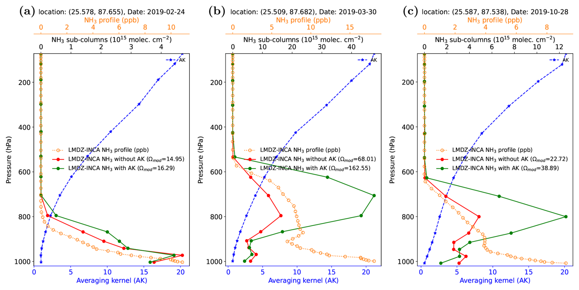
Figure 1 An example illustrating the convolution of LMDZ-INCA NH₃ vertical profiles with the IASI-ANNI-NH3-v4 averaging kernels (AK) to calculate the convolved LMDZ-INCA modeled NH₃ total column (Ω_mod). The LMDZ-INCA simulated original NH₃ mole fraction vertical profile (in ppb) at 79 model levels (represented by the orange dashed line on the secondary x axis at the top) and the AKs from individual IASI NH₃ pixels (represented by the blue dashed line on the primary x axis at the bottom) within a model grid cell centered at (25.5, 87.6) in India on three dates: (a) 24 February 2019, (b) 30 March 2019, and (c) 28 October 2019, and the corresponding NH₃ sub-columns (in molecules cm⁻²) (secondary x axis at the top) from the NH₃ vertical profiles simulated by LMDZ-INCA in this grid cell interpolated on the vertical levels of the assumed NH₃ profile in the IASI retrievals (shown in red) and the convolved LMDZ-INCA sub-column profiles with the AK (displayed in green). The values of Ω_mod with and without using the AK (in molecules cm⁻²) are also presented on the respective sub-plots for each day.

At a given hourly output of the model simulations with the IASI observations from the morning overpass around 09:30 LST, we derive a corresponding LMDZ-INCA NH₃ profile for each individual IASI NH₃ pixel within a model grid cell that contains the center of this pixel and derive the convolved LMDZ-INCA modeled NH₃ total column by applying the corresponding AK. Because the IASI resolution is much finer than that of LMDZ-INCA, this process yields several convolved modeled NH₃ total columns for a single model grid cell. We then average these resulting observed (Ω_obs) and corresponding AK-convolved modeled (Ω_mod) NH₃ total columns at the model spatial resolution (1.27° × 2.5°) for a proper comparison at the coarsest resolution between the two products. We exclude the grids of the averaged NH₃ total columns from the analysis if there are fewer than four high-quality IASI pixels within a model spatial grid or if the grid-cell average of observations is negative due to some negative IASI NH₃ total column retrievals.

2.4 Inversion of the global NH₃ emission from IASI observations

We use the finite difference mass-balance (FDMB) inversion approach (Cooper et al., 2017; Lamsal et al., 2011) for the global inversion of NH₃ emissions using NH₃ total columns from the LMDZ-INCA model simulations and IASI NH₃ observations. The inversion approach assumes that the short lifetime of NH₃ of a few hours to a day in the atmosphere limits its horizontal transport on coarse grids and thus implicitly conducts local analysis, deriving local surface emissions (in a given model horizontal grid cell) based on local observations (corresponding the same model horizontal grid cell), even though it relies on full 4D (3D in space, 1D in time) simulations with LMDZ-INCA. The FDMB inversion approach relies on the estimation of the local sensitivities (β) of the simulations of NH₃ total columns to changes in the local NH₃ emission, addressing non-linear chemistry effects from the model simulations. It derives NH₃ emission estimates at each grid cell by scaling a priori NH₃ emission (here based on the anthropogenic emissions from the CEDS inventory), considering the local sensitivity of NH₃ simulations to changes in emission and the relative difference between the observed and modeled NH₃ total columns. Our objective is a daily estimate of 10 d running mean global anthropogenic NH₃ emissions over land. However, with only satellite NH₃ observations, it is challenging to distinguish between anthropogenic and natural sources. Therefore, our approach focuses solely on grid cells and days where and when the prior NH₃ emission inventory indicates that the emissions are dominated by the anthropogenic sources and where and when we have retained grid-cell averages of the IASI NH₃ observations (see Sect. 2.3). We use the daily combined anthropogenic NH₃ emissions from CEDS and fire emissions from the GFED4 inventories, which are derived from monthly data and uniformly distributed at the hourly scale within each day in the LMDZ-INCA simulations, as a priori emissions (E_a) in the inversions. We select the grid cells with dominating anthropogenic NH₃ emissions by identifying those where the ratio of anthropogenic NH₃ emissions to total NH₃ emissions (including anthropogenic, biogenic, and fire NH₃ emissions) is greater than 0.6. This selection of dominant anthropogenic emissions slightly alters their spatial distribution over the years from 2019 onward due to variations in fire emissions across different years. We compute a 10 d running average at each grid cell of the modeled and observed NH₃ total columns and of the a priori emissions to smooth out the daily fluctuations in observed NH₃ total columns and to increase the sample size and spatial coverage of the daily flux estimates. Following Cooper et al. (2017) and Lamsal et al. (2011), for a given day and over each model horizontal grid cell, the satellite-constrained NH₃ emission estimates (E_IASI) using the observed IASI NH₃ total columns (Ω_obs) and the modeled LMDZ-INCA columns convolved with the AKs (Ω_mod) corresponding to a priori NH₃ emission (E_a) used in the model simulations are calculated as:

$$\begin{array}{}\text{(2)}& E_{\mathrm{IASI}}=E_{\mathrm{a}}\left(\mathrm{1}+\mathit{\beta }{\displaystyle \frac{{\mathrm{\Omega }}_{\mathrm{obs}}-{\mathrm{\Omega }}_{\mathrm{mod}}}{{\mathrm{\Omega }}_{\mathrm{mod}}}}\right),\end{array}$$

where a unitless scaling factor β accounts for the local sensitivity of the modeled NH₃ total columns ($\mathrm{\Delta }{\mathrm{\Omega }}_{\mathrm{mod}}/{\mathrm{\Omega }}_{\mathrm{mod}}$) to perturbations of the a priori NH₃ emissions ($\mathrm{\Delta }{E}_{\mathrm{a}}/E_{\mathrm{a}}$) and is defined as:

$$\begin{array}{}\text{(3)}& \mathit{\beta }={\displaystyle \frac{\mathrm{\Delta }{E}_{\mathrm{a}}/E_{\mathrm{a}}}{\mathrm{\Delta }{\mathrm{\Omega }}_{\mathrm{mod}}/{\mathrm{\Omega }}_{\mathrm{mod}}}}.\end{array}$$

We perform two LMDZ-INCA model simulations for each year: one using the prior emissions, with the anthropogenic NH₃ emissions from the CEDS bottom-up inventory for the year 2019, updated for subsequent years (see Sect. 2.2), and another with a 40 % reduction in the CEDS anthropogenic NH₃ emissions to derive β. We apply some filters to β, to the observed and/or the modeled NH₃ total columns, and/or to the bottom-up emissions to select the grids corresponding to the dominating anthropogenic emissions and to avoid negative or extreme unrealistic estimates of the NH₃ emissions from the inversions. We select grids over land only for (i) $\mathrm{0}\le \mathit{\beta }\le \mathrm{10}$, (ii) $\mathit{\beta }\frac{{\mathrm{\Omega }}_{\mathrm{obs}}-{\mathrm{\Omega }}_{\mathrm{mod}}}{{\mathrm{\Omega }}_{\mathrm{mod}}}\ge -\mathrm{1}$, and (iii) Ω_mod and ${\mathrm{\Omega }}_{\mathrm{obs}}>\mathrm{1}\times {\mathrm{10}}^{\mathrm{15}}$ molecules cm⁻². Figure S2 in the supporting information shows an example of the distribution of monthly mean values of β for July 2019. The values of β are less than 1.5 over most of the major NH₃-emitting land regions worldwide.

Satellite data gaps and some filters applied to observations and different variables in the FDMB inversion approach to focus on model grid cells dominated by anthropogenic NH₃ emissions result in numerous grids or days where NH₃ emissions could not be derived directly from the IASI NH₃ observations. Therefore, the derivation of national or regional budgets of anthropogenic emissions at daily (10 d scale) to monthly and annual scale from the satellite observations requires a proper gap-filling of grid cell or days for which the inversion protocol does not yield emission estimates. To fill these gaps in IASI-constrained NH₃ emissions, we use a rather conservative approach utilizing IASI-constrained NH₃ emissions and the corresponding a priori CEDS anthropogenic NH₃ emissions used in the inversions. The gap-filling is performed over some specific regions. In order to gap-fill the daily unconstrained NH₃ emissions, we compute a daily scaling factor as a ratio between the IASI-constrained and the corresponding CEDS anthropogenic NH₃ emissions integrated over a specific region. The missing emissions in that selected region are gap-filled by multiplying for each corresponding grid cell the CEDS NH₃ emissions with these scaling factors. For a given day, when the spatial coverage of the IASI-constrained anthropogenic NH₃ emissions is less than 60 % in a specific region due to poor satellite coverage and due to other data filtering to apply the FDMB inversion approach, we apply some constraints on the scaling factor to prevent spurious gap-filled emissions. If the IASI-constrained emissions coverage is less than 10 %, we directly use the prior CEDS NH₃ emissions. For coverage between 10 % and 40 %, we cap the scaling factor at 1.25, and for coverage between 40 % and 60 %, we cap it at 1.5. For the gap-filling, we use 10 continental regions (illustrated in Fig. S3) over the main land worldwide as defined by Ge et al. (2022) based on 58 IPCC reference regions representing consistent regional climate features described in Iturbide et al. (2020). Ge et al. (2022) used the nine regions (except the “rest of the world” region) to access global and regional budgets and fluxes of atmospheric reactive N and S gases and aerosols. The fraction of the IASI-constrained and the gap-filled NH₃ emissions per season across six regions for each year from 2019 to 2022 in Fig. S4 shows that the gap-filling of emissions over most of the regions is mostly higher during winter and minimum during spring. However, in some regions such as India and Africa, the percentage of the gap-filled emissions to the total seasonal emissions is higher in summer compared to other seasons due to relatively smaller numbers of satellite observations, caused by higher cloud coverage during the monsoon season. The overall percentage of the gap-filled NH₃ emissions to the total emissions worldwide is maximum (up to ∼28 %) during winter and minimum (up to ∼11 %) during spring, and it ranges from ∼16 % to 19 % during summer and autumn (Fig. S4). However, because the attribution of the NH₃ emissions in winter to the total annual emissions is smaller compared to the other seasons, the total gap-filled emissions in winter are still lower than in the other seasons (Fig. S5).

3 Results

We present the results from the LMDZ-INCA model comparisons with satellite NH₃ observations and inversions of NH₃ emissions at both global and regional scales over land areas. For regional analysis, we select six major NH₃ source regions: India, China, Africa, Europe, North America, and South America (Fig. S6). We present and discuss our results across various temporal scales, ranging from daily to monthly, seasonal, and annual.

3.1 Model and satellite comparison of NH₃ total columns

We start by comparing the LMDZ-INCA model-simulated NH₃ total columns driven by the prior emissions and convolved with the AKs against the IASI NH₃ observations, with first a worldwide overview and then some focuses on regions over land. In addition to assessing global and regional mean comparisons between the modeled and the observed IASI NH₃ columns, we also calculate the Pearson's correlation coefficient (r) and root mean square error (RMSE) between the annual or monthly mean simulated and observed values at the model grid level as part of our comparative analysis (shown in Figs. 2 and 3 for 2019 and Fig. S7 for all years from 2019 to 2022).

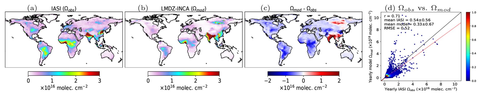
Figure 2 The spatial distributions of the annual mean NH₃ total columns (in molecules cm⁻²) for the year 2019 (a) from the IASI-ANNI-NH3-v4 observations (Ω_obs) and (b) from LMDZ-INCA model-simulated columns after applying the averaging kernel (Ω_mod), as well as (c) the difference (Ω_mod−Ω_obs) between them. The last column (d) shows the scatter density plots between these annual mean observed IASI and the corresponding LMDZ-INCA model NH₃ columns across all model grid cells worldwide over land. In the scatter plots, the solid black line represents the one-to-one line, while the dashed red line represents the regression line.

Figure 2 compares the annual mean modeled LMDZ-INCA NH₃ columns (Ω_mod) with the observed IASI NH₃ column retrievals (Ω_obs) regridded on the LMDZ-INCA model grid (1.27° × 2.5°) worldwide over land for the year 2019 (Fig. S7 for all 4 years from 2019 to 2022). It shows that the annual mean worldwide spatial distributions of the modeled NH₃ columns are approximately similar to those of the IASI NH₃ retrievals and that there is a good spatial correlation (r=0.71) between them. However, the IASI NH₃ observations indicate higher NH₃ abundance compared to the LMDZ-INCA simulations across most of the regions worldwide, except over the South Asia and Eastern Siberia regions (Fig. 2). We observe an overall underestimation of the global annual mean LMDZ-INCA NH₃ columns Ω_mod (mean: 0.33×10¹⁶ molecules cm⁻²) compared with the observed IASI retrievals Ω_obs (mean: 0.54×10¹⁶ molecules cm⁻²). The RMSE between the annual mean gridded Ω_mod and Ω_obs worldwide is 0.52×10¹⁶ molecules cm⁻².

Emphasizing the regional analysis, in Fig. 3, we found that the modeled NH₃ total columns are lower than the IASI NH₃ observations over most of the selected regions, except over the Indian region (also Southeast Asia, not shown; see Fig. 2), and also over a region in Eastern Siberia, where the model shows an overestimation of the observations (not shown, but see Fig. 2). The annual regional mean of monthly Ω_mod over the China, Africa, Europe, South America, and North America regions are respectively ∼4 %, ∼52 %, ∼53 %, ∼58 %, and ∼70 % smaller compared to Ω_obs (Fig. 2). However, over the Indian region, the annual regional mean of Ω_mod is ∼44 % larger than Ω_obs. The monthly regional mean time series of the IASI NH₃ observations in Fig. 3 show that the NH₃ columnar abundance over most of the regions is higher during spring and/or summer months compared than in winter. These elevated NH₃ columns observed during spring and/or summer months compared to winter months can be attributed to increased agricultural activities, particularly the prominent use of N-fertilizers in crops during warmer seasons. High NH₃ concentrations are also influenced by temperature, as warmer temperatures can enhance NH₃ volatilization from soils and agricultural surfaces (Sutton et al., 2013). This synergistic effect of agricultural practices and temperature contributes to the seasonal variation in NH₃ emissions, with higher concentrations during spring and/or summer months.

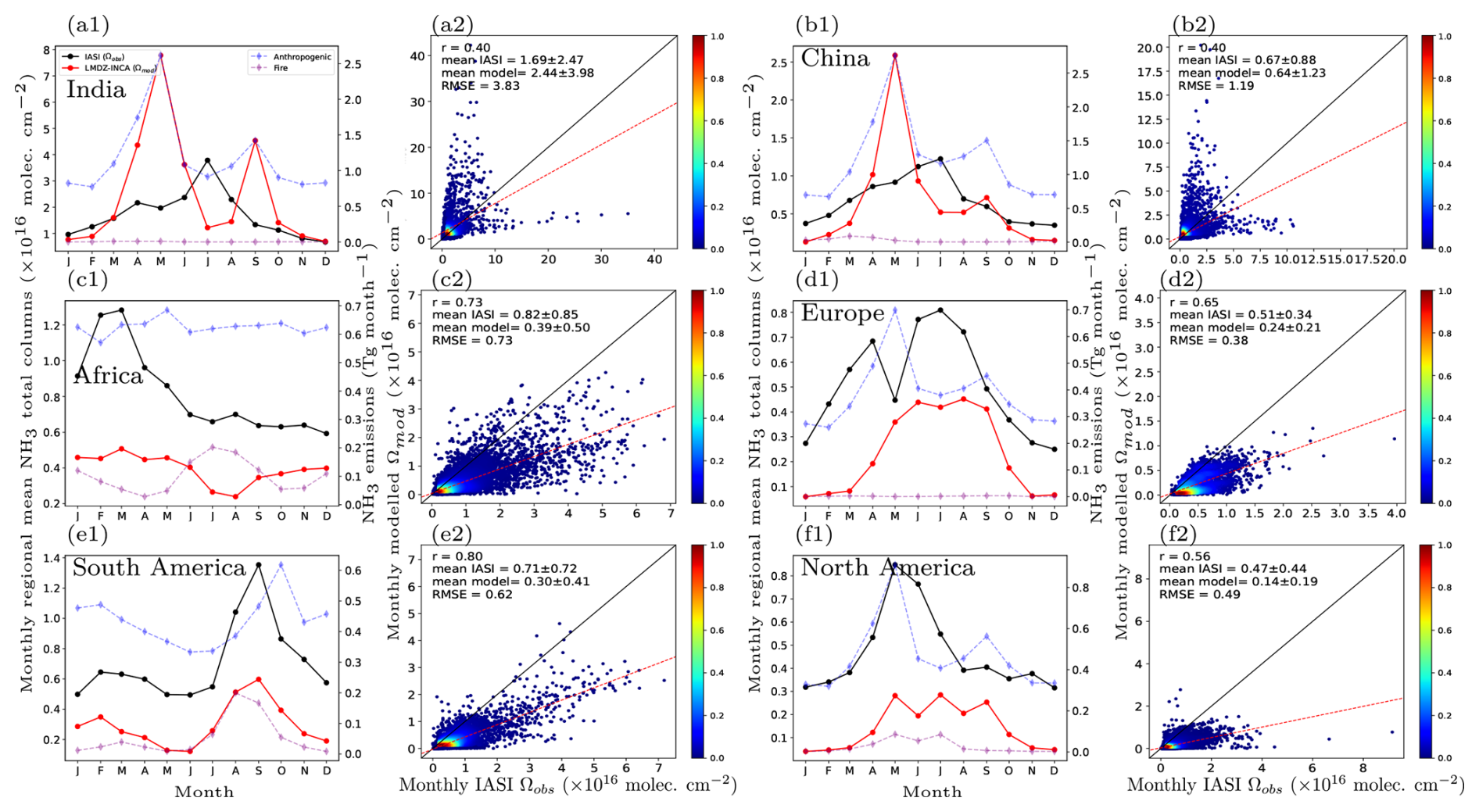
Figure 3 The monthly regional mean time series of the observed IASI NH₃ total columns (Ω_obs), the corresponding LMDZ-INCA modeled columns (Ω_mod) (primary y axis), and the monthly anthropogenic (CEDS) and fire (GFED4) NH₃ emissions (secondary y axis) from bottom-up inventories used in the model simulations for the year 2019 for different selected regions: (a) India, (b) China, (c) Africa, (d) Europe, (e) South America, and (f) North America (first column). The second column in each subfigure shows the scatter density plots between the monthly mean gridded observed IASI and the corresponding modeled NH₃ total columns over the land grid cells at 1.27° × 2.5° resolution in each region. In the scatter plot, the solid black lines represent the one-to-one line, while the dashed red lines represent the regression line.

The monthly regional mean modeled NH₃ columns in Fig. 3 mostly follow the seasonal variation of the IASI observations over the South American and African regions, as well as over the European region to some extent. However, for other remaining regions, especially over the Indian, Chinese, and Middle East (not shown) regions, the seasonality of the modeled NH₃ columns largely deviates from the observations, and we see a large scatter between the monthly mean gridded modeled and observed NH₃ columns (Fig. 3a and b). Over the Indian region, the model shows two main peaks, with the highest peak in May following a secondary smaller peak in September, whereas the IASI observations show the highest peak in July and a smaller one in April (Fig. 3a1). The high NH₃ loading from the IASI observations over the Indian region from June to August with a maximum peak in July and a secondary, much smaller peak in April (Fig. 3a1) is consistent with the cropping cycle (Kuttippurath et al., 2020), high usage of the N-fertilizers, and high temperature during these monsoon and summer months in the Indo-Gangetic Plain (IGP) region spanning the banks of the Indus and Ganges rivers and their tributaries (Beale et al., 2022). However, as mentioned before, the variation and two distinct peaks in the modeled NH₃ columns is similar to the variation and peaks in the anthropogenic NH₃ emissions used in the model simulations (Fig. 3). Similarly, over the Chinese region, the observed NH₃ columns show the highest peak in July, which is not captured by the simulations that show the maximum peak in May, followed by a small peak in September. In these regions, because of differences in seasonal variations between the modeled and observed NH₃ columns, we see weak spatial correlations between the monthly mean observed and modeled gridded NH₃ columns (Fig. 3) that are smaller than in other regions like Africa, South America, and Europe, where the seasonality in both the modeled and observed NH₃ total columns is roughly similar.

Figure 3 also shows the seasonal cycles in the regional anthropogenic (CEDS) and fire (GFED4) emissions from the global emission inventories used in the model simulations. Over some regions like South America, North America, and Africa, fire-related NH₃ emission has a visible contribution to this seasonal variation in total emissions, whereas over the India, China, and European regions, this attribution is very small (Fig. 3). This finding shows that the seasonality in the modeled NH₃ total columns mostly varies with the seasonality in the combined anthropogenic and fire-related NH₃ emissions over these regions (Fig. 3). Therefore, the seasonality differences between the model and observations over some regions are mostly due to the different seasonality embedded in the prior NH₃ emissions used for the model simulations (Fig. 3). The model comparison analysis for other years from 2020 to 2022 shows a similar behavior of the modeled and observed NH₃ columns. Notably, the seasonality of anthropogenic NH₃ emissions in the CEDS inventory is mainly derived according to the European agricultural practices based on the ECLIPSE v5 model, which leads to NH₃ emission peaks mostly in May and September corresponding to the application of fertilizers before planting and after harvesting the crops (Beale et al., 2022). However, this seasonal variation of the NH₃ emissions in CEDS may not accurately reflect the diverse agricultural practices in other regions like India, China, and the Middle East (Fig. 3) (Beale et al., 2022; Chen et al., 2023a; Kuttippurath et al., 2020). This is clearly evident from the large difference in the seasonal variations between the IASI NH₃ observations and LMDZ-INCA model simulations over these regions, as the model is dominatingly driven by the CEDS anthropogenic NH₃ emissions in these regions (Fig. 3). This dependency on European seasonality in CEDS inventory NH₃ emissions for other major agricultural NH₃-emission regions with diverse agricultural practices, like India and China, requires region-specific data to improve the accuracy of emission inventories. For some regions like South America, Africa, and North America, the observed IASI NH₃ total columns show high values during specific periods, which is mainly attributed to the heightened NH₃ loading resulting from biomass burning from wildfires in these regions. The underestimation and/or distinct seasonality of the modeled NH₃ columns compared to the observed IASI NH₃ retrievals over different regions indicate biases and/or differential seasonality in the prior NH₃ emissions from the inventories over these regions.

Previous validation studies of earlier IASI ANNI NH₃ retrieval products (e.g., with version 3) showed relatively good agreement with in situ and FTIR measurements (Guo et al., 2021; Wang et al., 2020). Although, the IASI-ANNI-NH3-v4 product introduces important improvements compared to the earlier versions and expects minimal biases, a comprehensive validation of this version has not yet been conducted, though such a validation is anticipated in upcoming studies (Clarisse et al., 2023). Therefore, the bias between the IASI NH₃ columns and LMDZ-INCA model simulations mainly reflects an underestimation of agricultural NH₃ emissions in the prior CEDS inventory, as well as a misrepresentation of their seasonal variation, particularly in the major agricultural regions. These limitations in the prior CEDS NH₃ emissions propagates into the model-simulated NH₃ columns. However, the elevated NH₃ columns observed by IASI during non-growing seasons in regions such as Europe and North America may also be influenced by retrieval uncertainties related to surface temperature effects and low thermal contrast. Therefore, we cannot fully rule out remaining retrieval uncertainties in the absence of comprehensive validation of this version of the IASI NH₃ retrievals.

3.2 Evaluation of the estimated NH₃ emissions derived from inversions with the IASI NH₃ observations

In order to validate our atmospheric inversion approach (more specifically, to validate the linear approximation of the atmospheric chemistry model based on a single perturbed emission simulation) and strengthen our confidence in the NH₃ emission estimates, we have conducted a LMDZ-INCA model simulation using the IASI-constrained NH₃ emission estimates derived from our global inversions for the year 2019 and compared the simulated NH₃ total columns with the IASI NH₃ total column observations. As the current LMDZ-INCA model framework only reads NH₃ emissions at monthly resolution and uniformly distributes them across hours without incorporating diurnal or day-to-day variability (see Sect. 2.2), our model simulation for this evaluation uses the monthly average of the daily (at 10 d scale) inversion estimates rather than 1 d resolution inputs. However, this does not limit our capability to evaluate the inversion estimates based on comparisons to monthly and annual averages of the observations.

At the annual scale globally, the spatial correlation coefficient (r) between the yearly mean model-simulated NH₃ total columns over the model horizontal land grid cells at 1.27° × 2.5° resolution and corresponding IASI NH₃ observations improve from 0.71 (using prior emissions) to 0.90 (using IASI-constrained NH₃ emissions), while the RMSE decreases by ∼29 % from 0.52×10¹⁶ to 0.37×10¹⁶ molecules cm⁻² (Fig. S8a). Similarly, at the monthly scale globally, the r value and RMSE between the model simulations with the IASI-constrained NH₃ emissions and the IASI observations improve from 0.51 (using prior emissions) to 0.83 (using IASI-constrained NH₃ emissions), while the RMSE decreases by ∼34 % from 0.88×10¹⁶ to 0.58×10¹⁶ molec. cm⁻² (Fig. S8b). The LMDZ-INCA simulation driven by the IASI-constrained NH₃ emissions reduces the mean fractional bias (FB) globally from −0.87 to −0.37 at the annual scale and from −1.07 to −0.63 at the monthly scale, compared to the simulation using the prior CEDS NH₃ emissions (Fig. S8).

At the monthly scale and across major NH₃ regions, including India, China, Africa, Europe, South America, and North America, the spatial correlation coefficients (r) and RMSE between the model simulations with estimated NH₃ emissions from inversions and the IASI observations are respectively much higher and smaller than when the simulations are based on the prior CEDS anthropogenic NH₃ emissions (Fig. 4). The spatial correlation coefficient (r) between the monthly mean IASI-constrained NH₃ emissions' model simulations of the NH₃ total columns over the model horizontal land grid cells at 1.27° × 2.5° resolution and the corresponding IASI NH₃ observations exceeds ∼0.8 in most of the regions for this 2019 validation analysis (Fig. 4). In one of the major NH₃-emission regions, i.e., India, at the monthly scale, the spatial correlation increases from 0.40 to 0.86, and RMSE reduces by ∼50 % from 3.83×10¹⁶ to 1.91×10¹⁶ molec. cm⁻² (Fig. 4). Similarly, over another major NH₃-emission region, i.e., China, at the monthly scale, the spatial correlation increases from 0.40 to 0.79, and RMSE reduces by ∼27 % from 1.19×10¹⁶ to 0.87×10¹⁶ molec. cm⁻² (Fig. 4). These findings demonstrate the general improvement brought about at different spatiotemporal scales by the update of the emission estimates from our inversions and thus the internal consistency of our global inversion framework despite the rather simple linearization of the chemistry transport underlying it. This improvement of the fit to the IASI NH₃ observations is a strong indication of the robustness of our inversion-based estimate of the global NH₃ emissions. The FB metric quantitatively confirms bias reduction in the modeled NH₃ columns regionally when using IASI-constrained NH₃ emissions in the model simulation compared to the prior CEDS NH₃ emissions (Fig. S9). Specifically, we observe a clear decrease in FB across all regions, except for India. In the case of India, although the FB remains slightly elevated, the RMSE shows substantial improvement, indicating better representation of the magnitude and the spatial and temporal variability, even if the mean offset is not fully corrected from our inversion estimates.

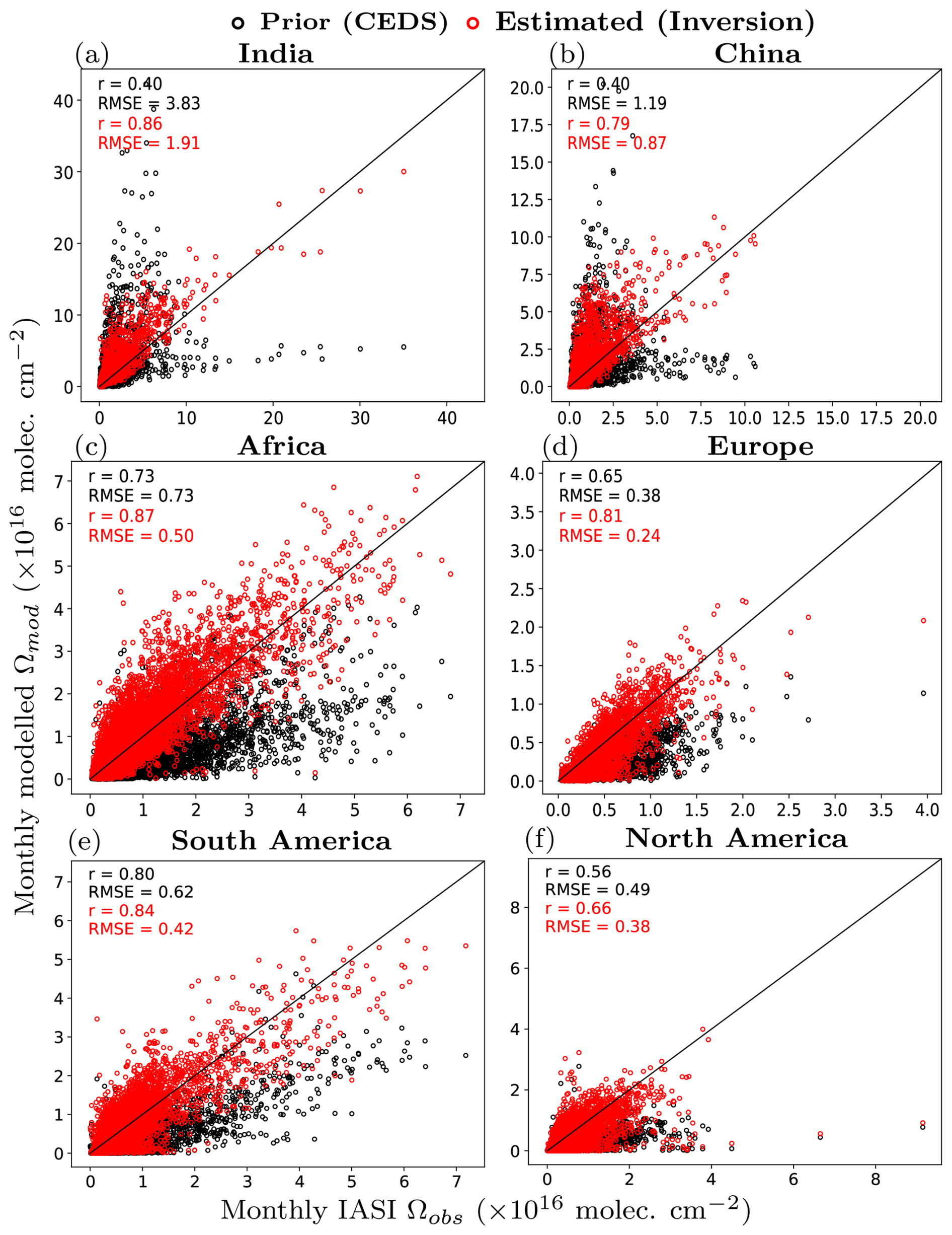
Figure 4 Comparison of the monthly averages of the gridded IASI NH₃ column observations (Ω_obs) over the model horizontal land grid cells at 1.27° × 2.5° resolution to the corresponding averages of these observations with two simulations of LMDZ-INCA (Ω_mod) using the IASI-constrained NH₃ emission estimates derived from our global inversions (red) and using the prior CEDS NH₃ emissions (black) over different regions for the year 2019. Each panel shows the correlation coefficient (r) and root mean square error (RMSE) between modeled (from both prior and IASI-constrained NH₃ emissions from inversions) and observed IASI NH₃ columns. The black line denotes the one-to-one line.

3.3 IASI-constrained NH₃ emissions

In the subsequent subsections, we present and discuss the gap-filled global daily (10 d scale) NH₃ emission estimates integrated on different temporal and spatial scales. Over the 4-year period of our emission estimates, we present global and regional annual budgets, including the mean emissions over this period, with the range defining minimum and maximum annual emissions, as well as the variation of the regional estimates at different temporal scales ranging from daily (10 d scale) to monthly, seasonal, and annual.

3.3.1 Global annual NH₃ emissions

The spatial distribution of the IASI-constrained annual NH₃ emissions averaged over the 4-year period (2019–2022) in Fig. 5 (Fig. S10 for each year from 2019 to 2022) clearly reveals the main hotspots of the high anthropogenic NH₃ emissions over the globe on land areas. Figure 5 shows that the 4-year-averaged annual IASI-constrained NH₃ emissions have a similar spatial distribution to the prior CEDS anthropogenic NH₃ emissions. However, over most of the major NH₃-emitting regions over the globe and over land areas, the IASI-constrained NH₃ emissions are higher compared to the prior CEDS emissions (Fig. 5). This finding shows that the South and East Asian regions are the highest anthropogenic NH₃-emitting regions over the globe.

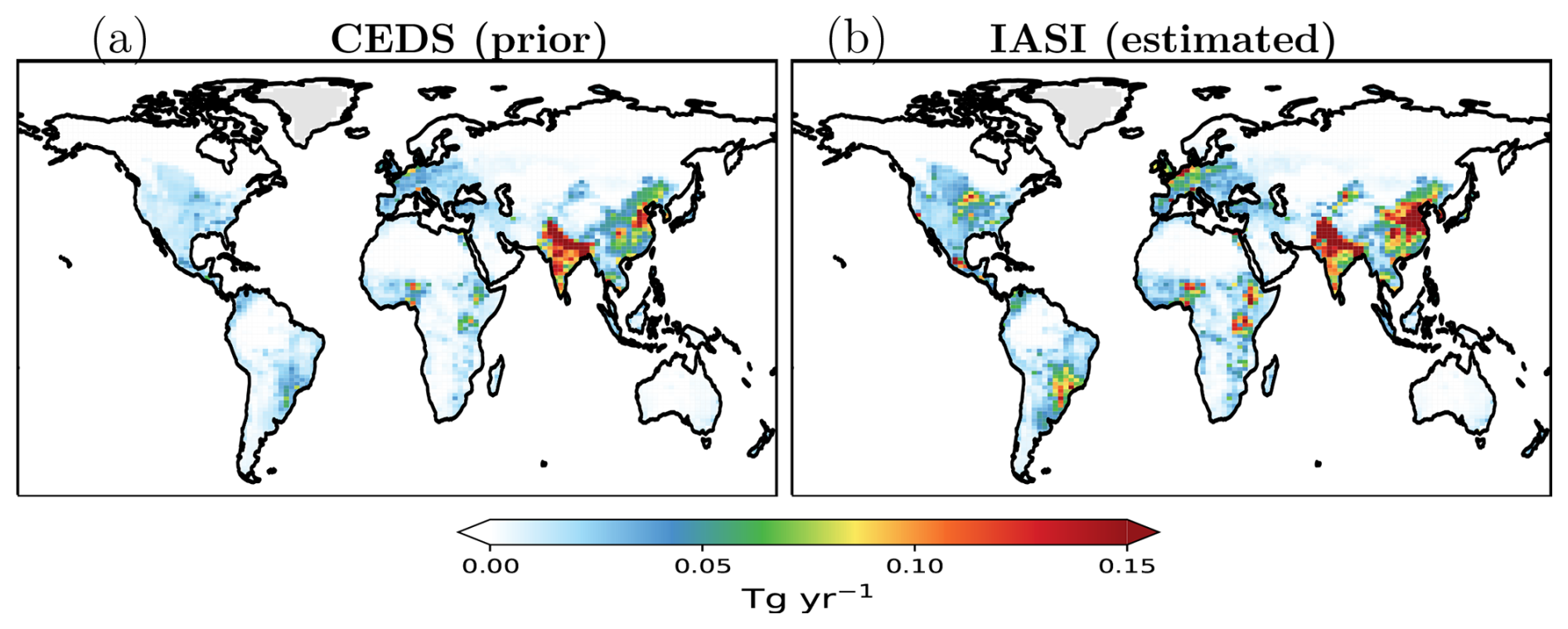
Figure 5 Spatial distribution of the 4-year (2019–2022) averaged annual NH₃ emissions, showing (a) the prior CEDS anthropogenic NH₃ emissions and (b) the IASI-constrained estimated NH₃ emissions from our global atmospheric inversions.

Figure 6 presents the global annual IASI-constrained NH₃ emissions and a comparison with the prior CEDS anthropogenic NH₃ emissions for all 4 years from 2019 to 2022. The slight differences in the prior CEDS emissions over the 4 years are mainly due to the different coverages of the dominating anthropogenic NH₃ emissions based on the CEDS anthropogenic and GFED fire emissions (see Sect. 2.4). For each year, the IASI-constrained NH₃ emissions are higher than the prior CEDS emissions. The average of the global annual NH₃ emission estimates over the 4-year period is ∼97 (93.8–99.9) Tg yr⁻¹, which is ∼61 % (55 %–65 %) higher than the prior CEDS anthropogenic NH₃ emissions. The global annual NH₃ emission estimates show an increasing trend from the year 2019 to 2021 (Fig. 6). However, NH₃ emission estimates for 2022 (∼96 Tg yr⁻¹) are lower than those for 2020 and 2021, though still higher than those for 2019 (∼94 Tg yr⁻¹).

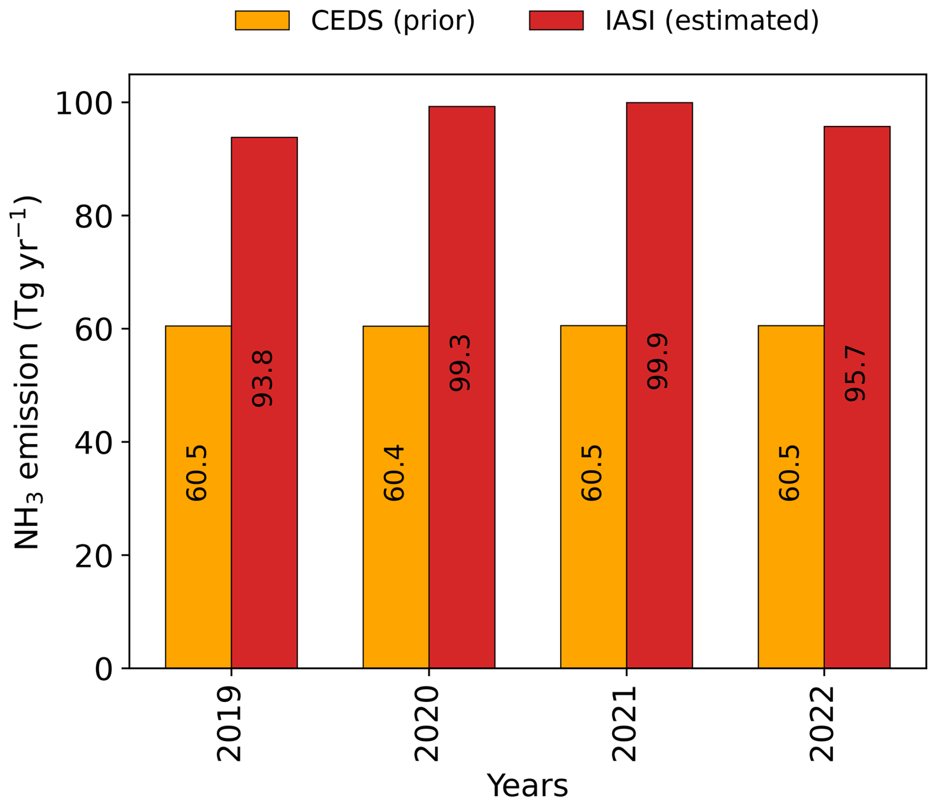
Figure 6 Global annual NH₃ emissions for each year from 2019 to 2022, showing the prior CEDS anthropogenic NH₃ emissions (orange) and IASI-constrained (red) NH₃ emissions from inversions.

3.3.2 Regional NH₃ emissions and seasonal variation

Figure 7 illustrates the daily (at 10 d scale) variation of estimated NH₃ emissions for 4 years from 2019 to 2022 over the six specific regions, i.e., India, China, Africa, Europe, North America, and South America (defined in Fig. S6), which have the major anthropogenic ammonia emissions. In this figure, the prior CEDS anthropogenic NH₃ emissions of the year 2019 over the globe and over land areas are almost the same in magnitude and seasonal variation across the 4 years (Fig. 6), and thus the representation is shown only for the year 2019. Figure 8 shows the spatial distributions of the 4-year-averaged annual IASI-constrained NH₃ emissions and the prior CEDS emissions over the six regions. The budgets of the regional annual estimated and prior NH₃ emissions over the 4-year period for these selected regions are presented in Fig. 9.

The Indian and Chinese regions in the South and East Asia are the major anthropogenic ammonia-emitting regions in the world, with a majority of emissions originating from large crop-specific agriculture activities, including the use of synthetic fertilizers, manure, and emissions from soils and livestock. Over the Indian region, the highest NH₃ emission is from the Indo-Gangetic Plain region, which is attributed to the intensive agriculture practices (Fig. 8a). The average annual NH₃ emission estimate for the 4-year period over the Indian region is ∼ 15.0 (14.4–15.4) Tg yr⁻¹, which is ∼7 % (∼2 %–10 %) higher than the prior CEDS anthropogenic NH₃ emissions (∼14.1 Tg yr⁻¹). The annual estimates over the Indian region show a slowly decreasing trend over the 4-year period (Fig. 9a). Notably, the seasonal variations of the estimated NH₃ emissions across all 4 years are similar to each other; however, they are always different from the prior CEDS NH₃ emissions (Fig. 7a). The seasonal variation in NH₃ emissions across different regions in the CEDS inventory dataset is rather coarse (Beaudor et al., 2023) and mostly based on the European practices of agricultural activities (Beale et al., 2022). The CEDS NH₃ emissions show two peaks, one in May and one in September, whereas the estimates show the main peak in July and August and some small peaks from January to April for each inversion year. The high NH₃ emission estimates over the Indian region for July–August with a peak in July are consistent with the cropping cycle (mainly rice cultivation followed by corn), high usage of N-fertilizers, and high temperature during these monsoon and summer months in the Indo-Gangetic Plain region. The high estimates in the winter and spring months can be attributed to the usage of N-fertilizers during the winter and spring crop seasons, particularly from the predominant wheat cultivation. Biomass burning is also a small contributing source of NH₃ emissions in this region, with the majority of fires resulting from crop residue and stubble burning in the spring and autumn before replanting. Therefore, there should not be a significant problem of attribution between the anthropogenic and biomass burning emissions here.

The majority of IASI-constrained and prior CEDS anthropogenic NH₃ emissions over the Chinese region are confined to the East China region (Fig. 8b). The 4-year average of inverted annual NH₃ emission over the Chinese region is ∼23.4 (22.3–24.9) Tg yr⁻¹ (Fig. 9b). This averaged IASI-constrained NH₃ emission is ∼62 % (∼54 %–72 %) higher than the prior CEDS emissions (∼14.5 Tg yr⁻¹) used in the inversions. For this region, we see an increasing trend in the estimated ammonia emissions from 2019 to 2021 (Fig. 9b). The annual NH₃ emission estimate for 2022 (23.2 Tg yr⁻¹) is lower than those for the maximum in 2021 (∼24.9 Tg yr⁻¹), comparable to those in 2020 (∼23.3 Tg yr⁻¹); however, it remains higher than those for 2019 (∼22.3 Tg yr⁻¹) (Fig. 9b). A majority of the ammonia emissions in this region originate from the crop-specific agriculture activities, more specifically the applications of synthetic fertilizer and livestock manure in different crop cultivations (Xu et al., 2018). The daily (at 10 d scale) variation of the NH₃ emissions in Fig. 7b shows a strong seasonality in the estimates across all years over this region. The seasonality in the emission estimates across all years is different from the prior CEDS NH₃ emissions used in the inversions. We observe mainly two high peaks in the estimates, one in spring (March–April) and one in summer (June–July), whereas the CEDS emissions show a peak in May and another in September. The NH₃ emission estimates also show a small third peak in October for inversion years from 2020 to 2022, except for 2019. The strong seasonality in the emission estimates in this region agrees well with the crop cycle when wheat cultivation dominates in spring and rice cultivation in the summer months (Xu et al., 2018).

As discussed before in Sect. 3.1, seasonality in the CEDS inventory NH₃ emissions for most of the regions is mostly based on European agricultural practices, corresponding to the application of fertilizers before planting and after harvest (Beale et al., 2022). This does not accurately capture the NH₃ emissions in regions like China, India, and the Middle East, where agriculture practices differ significantly (Beale et al., 2022; Chen et al., 2023a; Kuttippurath et al., 2020). By contrast, our inversion estimates based on the satellite data show more realistic seasonality of NH₃ emissions across different regions, closely aligning with their respective crop and agriculture cycles.

The South America, Africa, and North America regions are fire-dominated regions, particularly during the dry season, when wildfires are prevalent (Fig. S11) (Chen et al., 2023b). The biomass burning from the wildfires plays a significant role in contributing to the total ammonia emissions in these regions. For example, over the 4-year study period, biomass burning NH₃ emissions from GFED contribute ∼11 %–15 % in South America, ∼15 %–17 % in Africa, and ∼5 %, with a high peak of ∼26 % in 2021, in North America relative to the anthropogenic NH₃ emissions from the CEDS inventory. When fire emissions attribution in the prior emissions used for inversion is inaccurate, the predominant anthropogenic emission grids are misrepresented. In contrast, the IASI NH₃ observations will indicate high NH₃ emissions over these grid cells due to biomass burning. The recent release of the fifth version of the Global Fire Emissions Database (GFED5) indicates a 61 % increase in global burned area compared to GFED4 (Chen et al., 2023b). This increase may result in anthropogenic NH₃ grids from the inversions corresponding to biomass burning grids, consequently revealing heightened predominant anthropogenic NH₃ emission estimates over these regions due to a non-local contribution from transport from neighboring predominant biomass burning grids. Biomass burning generates NH₃ advection at higher altitudes, which also breaks our assumption of weak lateral transport in the FDMB inversion approach, possibly attributable to large errors in the emission estimates over these regions.

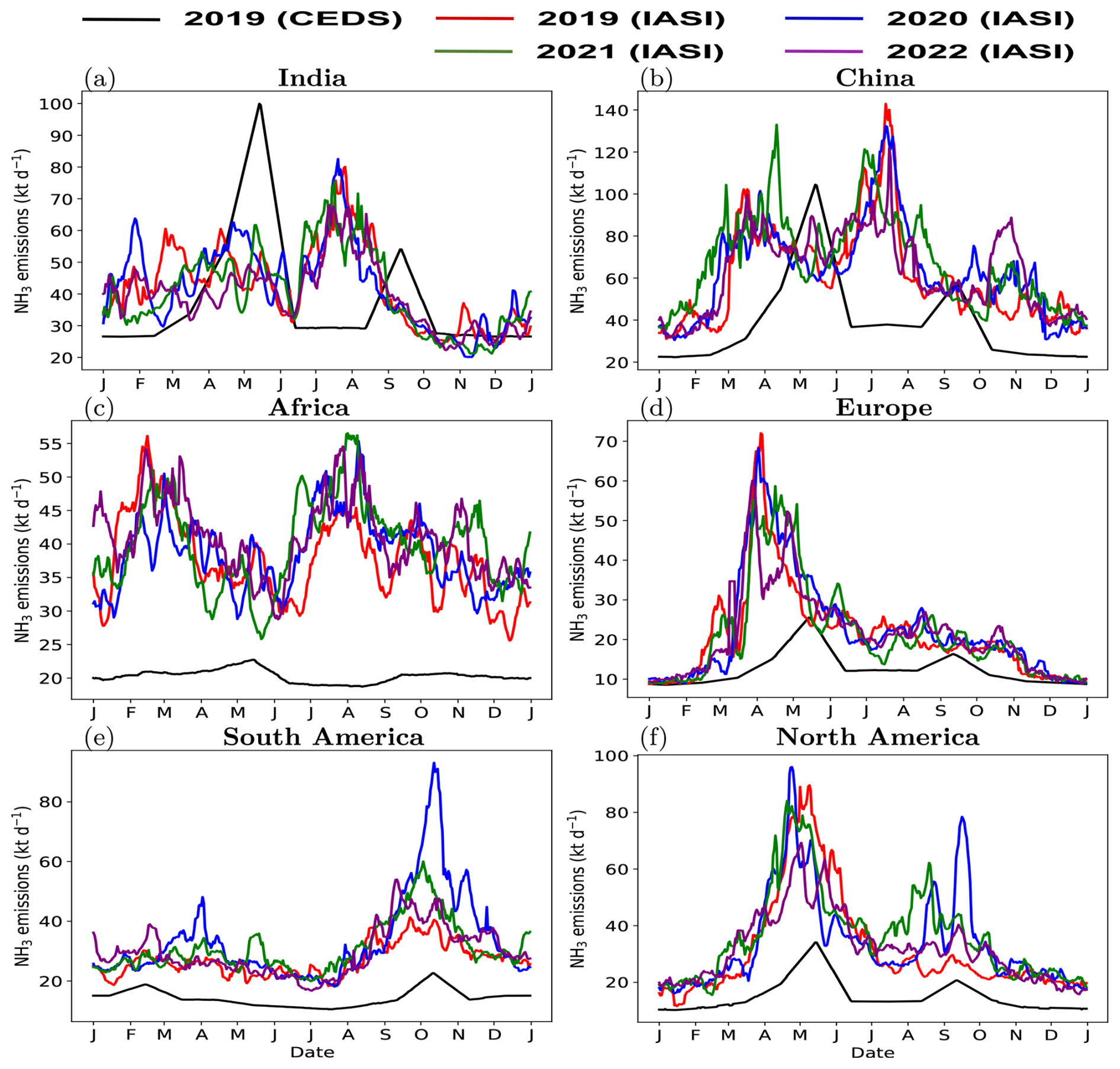
Figure 7 Daily (at 10 d scale) variation of the total estimated and the prior CEDS anthropogenic NH₃ emissions for the 4 years from 2019 to 2022 integrated over each selected region: (a) India, (b) China, (c) Africa, (d) Europe, (e) South America, and (f) North America.

For the South American and African regions, our inversions respectively provide ∼11.1 (∼9.8–12.3) Tg yr⁻¹ (Fig. 8e) and ∼14.4 (∼13.8–15.0) Tg yr⁻¹ (Fig. 9c) of the annual NH₃ emissions averaged over the 4-year period. These averaged annual estimates for these regions exceed the prior CEDS emissions by approximately 2.1 and 2 times, respectively. Our estimates show a clear increasing trend in annual NH₃ emission over Africa (Fig. 9c). However, a decreasing trend of annual NH₃ emissions from 2020 to 2022 is observed over the South American region (Fig. 9e). For the South American region, we observe a high peak in the estimated emissions during September to October in each year, and this peak in the year 2020 is much higher than that from other years (Fig. 7e). In fact, the peak in 2021 is higher than the one from the estimates in 2019 and 2022. The seasonality of the estimates over the South American region is similar to the prior CEDS anthropogenic NH₃ emissions (Fig. 7e). There was a large increase in the number of fires in 2020 compared to other years in this region (Fig. S11a), which can also be observed from an enhanced observed NH₃ loading from IASI observations over this region in these years (Fig. S7). The highest peak in the estimated NH₃ emissions in 2020 is mainly because of the contribution from the relatively higher number of fire occurrences in this year. For the African region, the prior CEDS NH₃ emissions show almost a flat seasonality relative to the estimates, with a small peak in May, whereas the estimates show at least two clear peaks: in February–March and in July–August (Fig. 7c). The NH₃ emissions over this region remain high during other seasons also (Fig. 7c). Although we exclude grids dominated by the biomass burning emissions based on the GFED4 bottom-up inventory in our inversions, mitigating their influence on the inversion estimates is challenging. This is due to the complexity arising from the fact that bottom-up NH₃ emissions lack the most updated information on fire occurrences, and the transport from biomass burning areas can extend to other regions, which is not accounted for in our inversion approach (Chen et al., 2023b).

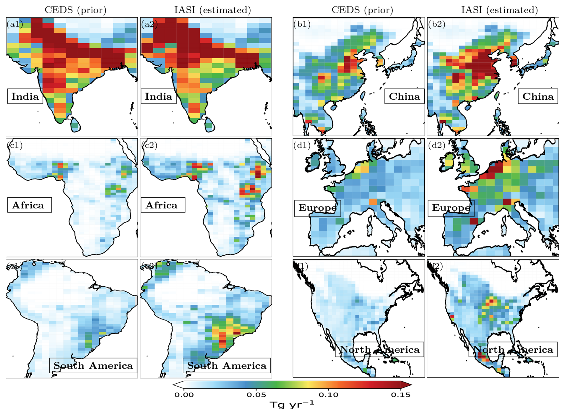
Figure 8 Spatial distribution of the total annual NH₃ emissions averaged over the 4-year period (2019–2022) across six regions, i.e., (a) India, (b) China, (c) Africa, (d) Europe, (e) North America, and (f) South America, showing bottom-up prior CEDS emissions (first column) and IASI-constrained estimated emissions (E_IASI) using the IASI NH₃ observations (Ω_obs).

We estimate ∼12.4 (11.6–13.4) Tg yr⁻¹ 4-year-averaged annual NH₃ emissions over the North American region, which is approximately 2.2 times higher than the prior CEDS anthropogenic NH₃ emissions (Fig. 9f). Our inversion estimates show an increasing trend of annual NH₃ emissions from 2019 to 2021 over this region, but the 2022 estimates are smaller than those from 2020 and 2021 and comparable to the 2019 emissions (Fig. 9f). The estimates show a strong seasonality, with peak emissions in April–May across all years (Fig. 7f). For the years 2020 to 2022, especially for 2020 and 2021, we observe a secondary peak during August and September, which is less visible in the 2019 emissions. The high secondary peak in 2020 and 2021 may result from increased biomass burning due to more wildfires in these years compared to 2019. Similar to the South American and African regions, in the North American region, the impact of biomass burning from fires from some regions may contribute to the higher ammonia emissions (Fig. S11c). In fact, the highest peak in the estimated emissions in 2020 in this region corresponds to an extreme cluster of wildfire events known as the “August Complex Fire”. This event originated as 38 separate fires started by lightning strikes on 16–17 August 2020 in the western U.S., leading to the first “gigafire” event in modern history in California (Campbell et al., 2022; Makkaroon et al., 2023). Campbell et al. (2022) showed that this 2020 “gigafire” contributed up to 83 % of the total nitrogen emissions in the western U.S. However, based on the GFED4 inventory fire emissions, our inversion could not filter out the grids dominated by these wildfire emissions during such events in this region.

Over the European region, hotspot regions with high anthropogenic NH₃ emissions are well detected from our inversion estimates (Fig. 8d). The 4-year average of the annual NH₃ emission estimates over this region is estimated as ∼7.9 (7.7–8.2) Tg yr⁻¹ (Fig. 9d). The estimated annual emissions over this region in 2020 are higher than in the other remaining inversion years; however, the estimates still remain approximately comparable across these years (Fig. 9d). Our emission estimates over the European region are ∼72 % higher compared to the prior CEDS anthropogenic NH₃ emissions. The estimates show a strong seasonality across all years, with high emissions from March to May peaking in April (Fig. 7d). This seasonality in the estimates differs from the prior CEDS anthropogenic NH₃ emissions, which show a high peak in May and a smaller one in September (Fig. 7d). The strong seasonality in the emission estimates agrees well with the crop cycle over the European region when the main cultivation activities dominate in the spring and summer seasons.

Other than these selected regions, we also briefly analyze regional estimates over the Middle East region, a comparatively smaller ammonia-emitting region (Fig. S12). A recent study by Osipov et al. (2022) based on ship-borne measurements around the Arabian Peninsula and modeling showed that NH₃ emissions over the Middle East region are significantly underestimated, potentially by a factor exceeding 15, from the EDGAR inventory emission used in their model simulations. While natural sources of ammonia play a negligible role in this region, the vast majority of emissions arise from industrial and agricultural activities. Over the Middle East region, our average annual anthropogenic estimate of ∼4.4 Tg yr⁻¹ (∼ 4.4–4.5 Tg yr⁻¹) is approximately 49 % higher than the prior CEDS emissions (∼3.0 Tg yr⁻¹). The annual NH₃ emissions in these regions remained almost the same over the 4-year period (Fig. S12c). The estimated NH₃ emissions show strong seasonality, with a high peak in May–April and a second peak in July–August, across all four years, whereas the prior CEDS anthropogenic NH₃ emissions show two peaks: in May and in September (Fig. S12b).

4 Discussion

4.1 Comparison with bottom-up inventories and other NH₃ emission estimates

In this section, we compare our IASI-inverted NH₃ emission estimates with other global and regional bottom-up inventories, as well as with other available NH₃ emission inversion estimates reported in recent literature. We use two global bottom-up NH₃ emission inventories: (i) CAMS-GLOB-ANT v6.2 (developed by combining the CEDSv2 emission trends and temporal profiles from CAMS-GLOB-TEMPO and EDGAR v6 historical monthly NH₃ emission data up to 2018) 0.1° × 0.1° monthly dataset (Granier et al., 2019; Soulie et al., 2024) from 2019 to 2022 and (ii) the process-based agricultural and natural soil NH₃ emissions from the Calculation of AMmonia Emissions in ORCHIDEE (CAMEO) model at 1.27° × 2.5° horizontal and monthly temporal resolutions (Beaudor et al., 2023). CAMEO simulates NH₃ sources from the agricultural sector, from livestock manure management (from animal housing and manure storage to grazing) to synthetic and organic nitrogen application to soil. Because CAMEO emissions are not limited only to cultivated/livestock areas and are dynamically dependent on environmental conditions and atmospheric deposition, emissions from natural ecosystems are also exploited in this study. For these inter-comparisons, we regridded the global NH₃ emissions from the bottom-up inventories on the grids (1.27° × 2.5°) of our estimated emissions. We also sub-sampled the monthly emissions from the bottom-up inventories on the common grids corresponding to the IASI-constrained monthly NH₃ emissions derived from the daily (at 10 d scale) estimates. Note that CAMEO additionally includes natural soil NH₃ emissions, whereas CAMS emissions do not include them and provide only anthropogenic NH₃ emissions.

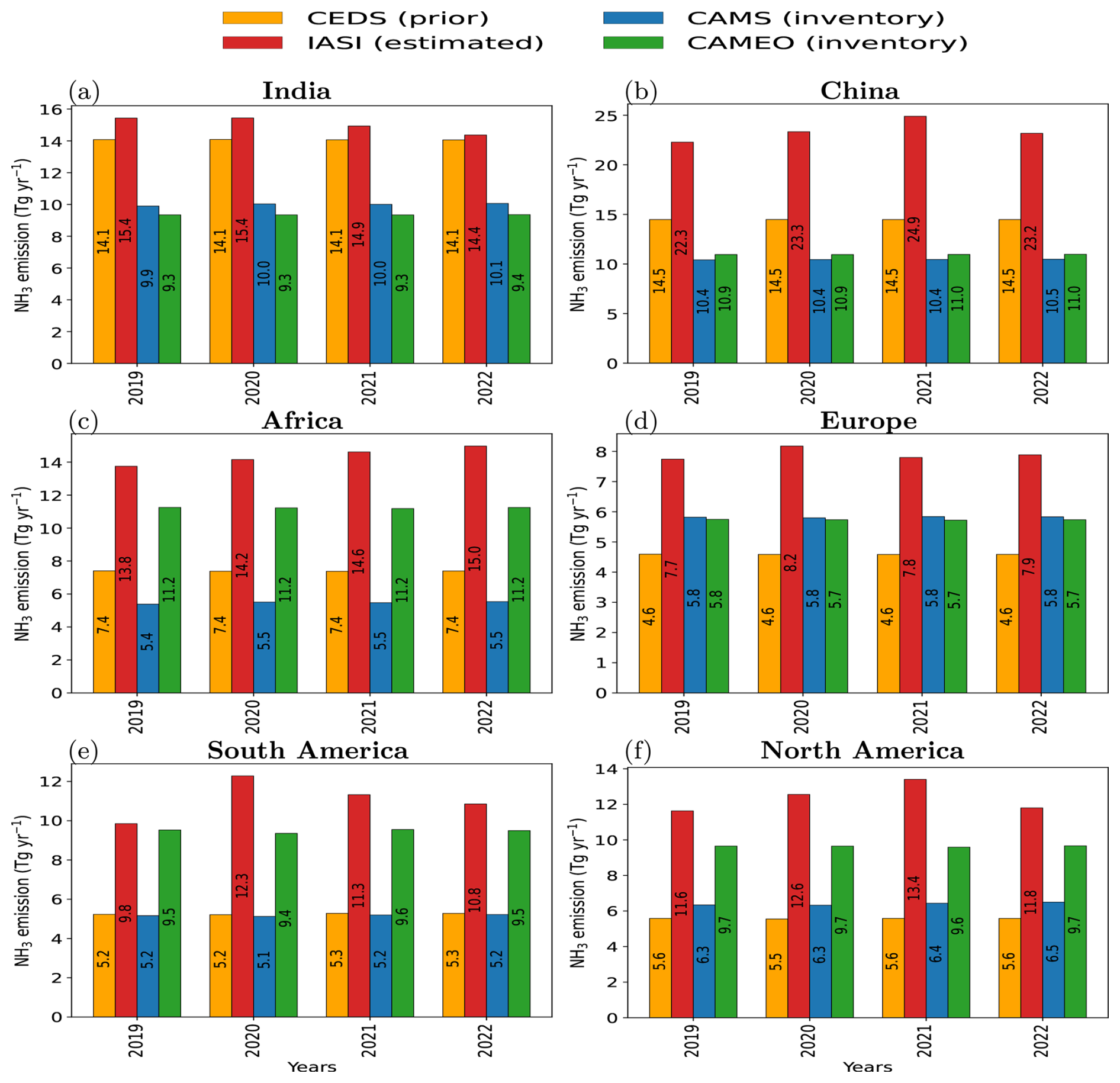
Figure 9 The regional annual NH₃ emissions spanning from 2019 to 2022 over the six regions over land areas, derived from the IASI-constrained daily global estimates, the prior CEDS inventory anthropogenic NH₃ emissions, and two independent global bottom-up inventories: CAMS (anthropogenic NH₃ emissions) and CAMEO (combined agriculture and natural soil NH₃ emissions). The CAMEO NH₃ emissions are for the last available year, 2014, selected on the common grids of each year's estimates.

The 4-year (2019–2022) average of the global annual anthropogenic NH₃ emissions from the CAMS bottom-up inventory (∼52.5 Tg yr⁻¹), sub-sampled on the common grids where the IASI-constrained monthly emissions are available, is lower than the prior CEDS anthropogenic NH₃ emissions (∼60.5 Tg yr⁻¹), whereas global annual NH₃ emissions from CAMEO from the combined agricultural and natural soil sectors (∼71.1 Tg yr⁻¹) are higher than those from both CEDS and CAMS. Therefore, we have an even larger relative difference between the estimated and the CAMS emissions than the relative difference between the estimated and CEDS emissions (Fig. 9). However, this relative difference between the estimated and CAMEO's combined agriculture and natural soil NH₃ emissions is smaller compared to the relative difference between the estimated and CEDS. The 4-year-averaged global annual NH₃ emissions from the inversions are ∼1.8 times higher than the CAMS anthropogenic NH₃ emissions and ∼1.4 times higher than the CAMEO combined agriculture and natural soil NH₃ emissions. Figure 9 shows a comparison between the IASI-inverted annual emissions and the corresponding CAMS and CAMEO emissions over six regions (and over the Middle East in Fig. S12) and across 4 years, revealing consistently higher IASI-constrained NH₃ emissions compared to these global bottom-up inventories.

We also compare our estimates with the recent global NH₃ inversion emission estimates by Luo et al. (2022) based on a previous version of IASI NH₃ observations from 2008 to 2018, with the recent estimates from Dammers et al. (2022) derived using the CrIS observations from 2013 to 2020, and with some other regional inversion estimates. Luo et al. (2022) estimated global annual NH₃ emissions at ∼78 (70–92) Tg yr⁻¹ averaged over a period from 2008 to 2018, and Dammers et al. (2022), over a period from 2013 to 2020, had 216.6±66.2 Tg yr⁻¹ (for all detected source locations) and 74.1±17.7 Tg yr⁻¹ (for inventory-identified source locations). Our averaged global annual NH₃ emission estimates of ∼97 (94–100) Tg yr⁻¹ from 2019 to 2022 are ∼25 % higher than the average total estimates (∼78 Tg yr⁻¹) from Luo et al. (2022). This can partly be explained by the fact that the IASI version 4 NH₃ column values used in this study are also about 10 %–20 % higher than the earlier version 3 (Clarisse et al., 2023) used by Luo et al. (2022) due to a reduction of the retrieval biases. This also has to be explained by the use of a different inversion approach, of a different chemistry transport model, and of AKs from IASI NH₃ observations to model-simulated NH₃ columns in this study. Our estimates align more closely with the upper range (∼92 Tg yr⁻¹) of their emission estimates obtained by setting a 200 % perturbation to the modeled atmospheric NH₃ lifetime in their inversions. It should be noted that Luo et al. (2022) corrected their NH₃ emissions over the Indian and the East China regions during 2013 to 2018, which were impacted by the rapid changes in SO₂ emissions and concentrations in these regions, especially the rapid decrease in SO₂ emissions over China. A decrease in SO₂ emissions leads to an increase in NH₃ concentrations/columns in the troposphere because lower SO₂ levels reduce the formation of ammonium sulfate aerosols, leaving more free ammonia in the atmosphere, which increases its concentration in the air (Luo et al., 2022). This correction in Luo et al. (2022) leads to a small increase in NH₃ emissions over the Indian region. However, a substantial reduction of ∼7–8 Tg for the year 2018 is observed over the East China region. Without any correction for SO₂ trends, our estimates (for 2019) are closer to their estimates for the year 2018. In contrast, our average total global estimate of ∼97 (93.8–99.9) Tg yr⁻¹ for the period 2019–2022 is ∼2.2 times smaller than the 216.6±66.2 Tg yr⁻¹ total from the sum of all detected source estimates from Dammers et al. (2022). Additionally, our 4-year-averaged estimates are ∼ 31 % higher when comparing with their estimates (74.1±17.7 Tg yr⁻¹) corresponding to the sources in the CAMS-GLOB-ANT v4.2 inventory emissions above the detection limit of their satellite-constrained emissions.

In order to compare our regional NH₃ emissions, derived from the global inversion estimates, with those of Luo et al. (2022), we regrid their final inversion year (2018) estimates to match the spatial resolution (1.27° × 2.5°) of our estimated NH₃ emissions. Subsequently, we integrate both the emission estimates over the identical grids on common selected regions' domains over land and compare their final inversion year's (2018) NH₃ emissions with our nearest first inversion year (2019) estimates. In comparison with Dammers et al. (2022), their regional estimates for all detected source locations are consistently higher than our estimates. Therefore, in the subsequent comparison analysis, we compare our estimates with only their regional reported estimates corresponding to the sources with inventory emissions above the detection limit of their satellite-derived emissions. This comparison is consistent, as our estimates also required information on the prior CEDS NH₃ emissions, and for the missing sources with zero emissions in the bottom-up inventory, our inversion will not detect any new emission sources. Over the Indian region, our annual estimates of 2019 (∼15.4 Tg yr⁻¹) are closer to the estimates of 2018 (∼13.1 Tg yr⁻¹) from Luo et al. (2022), representing a marginal ∼18 % increase. Our estimates over the China region of 2019 (22.3 Tg yr⁻¹) are much higher (∼73 %) compared to the Luo et al. (2022) SO₂ trend-corrected NH₃ emissions (∼13 Tg yr⁻¹); however, these are closer to their estimates without correction. Recently, Liu et al. (2022) estimated 21.6 Tg NH₃ yr⁻¹ (≡17.77 Tg N yr⁻¹) annual emissions over China for the year 2019 using satellite data, and our estimates (22.3 Tg yr⁻¹) for the same year are comparable to these inversion estimates. Dammers et al. (2022) reported ∼35 Tg yr⁻¹ average NH₃ emissions for the Asia region, and our combined 4-year-averaged estimate of ∼43 Tg yr⁻¹ from India, China, and the Middle East regions is ∼23 % higher than their estimate. Our estimates for Africa (∼13.8 Tg yr⁻¹), South America (∼9.8 Tg yr⁻¹), and the Middle East (∼4.4 Tg yr⁻¹) regions for 2019 agree well with the Luo et al. (2022) estimates (11.1, 10.5, and 4.1 Tg yr⁻¹, respectively) of 2018 within ∼24 %, ∼6 %, and ∼6 %, respectively. For the South American region, our annual estimate of ∼9.8 Tg yr⁻¹ for 2019 agrees well with the estimate of 9.1 Tg yr⁻¹ from Dammers et al. (2022). Our estimates (11.6 Tg yr⁻¹) for 2019 over the North American region are ∼55 % higher than ∼7.5 Tg yr⁻¹ from Luo et al. (2022); however, they are comparable to the total estimates of 12.2 Tg yr⁻¹ from Dammers et al. (2022). Recently, Sahoo et al. (2024) constructed a high-resolution gridded (0.1° × 0.1°) emission inventory of NH₃ emissions over India for 2022 by including 24 regional major and minor anthropogenic sources. They estimated 10.54 Tg yr⁻¹ of NH₃ emissions in 2022, which are closer to the CAMS anthropogenic NH₃ emissions, while our inversion estimates of 14.4 Tg yr⁻¹ NH₃ emissions for the same year are ∼ 36 % higher than their estimates (Fig. 9b). However, in this comparison analysis over the Indian region, our selected domain is larger, encompassing most of South Asia, compared to the India-only domain considered in Sahoo et al. (2024).

Over the European region, our annual NH₃ estimate (∼ 7.7 Tg yr⁻¹) for 2019 is ∼91 % higher compared to ∼ 4.1 Tg yr⁻¹ from Luo et al. (2022) for 2018. However, our 4-year-averaged annual estimates (∼7.9 Tg yr⁻¹) are ∼ 29 % smaller than ∼11.1 Tg yr⁻¹ from the estimates of Dammers et al. (2022). The European Union (EU) emission inventory report (EEA Report No 4/2023, 2023) reported comparatively lower NH₃ emissions for the EU 27 member states of 3.5, 3.4, and 3.3 Tg yr⁻¹ for 2019, 2020, and 2021, respectively, which are much lower compared to our estimates for these years. Also, some other recent top-down inversion studies, such as Tichý et al. (2023), have obtained a similar order of magnitude of the emissions (4.3 and 4.0 Tg yr⁻¹ for 2019 and 2020, respectively) using the CrIS satellite observations from Luo et al. (2022) (4.1 Tg yr⁻¹ for 2018) or from EEA Report No 4/2023 (2023). However, our estimates are comparable to the NH₃ emissions derived from a recent regional atmospheric inversion over Europe at 0.2° × 0.2° horizontal and monthly temporal resolutions over a 3-year period from 2020 to 2022, derived within the EU project Sentinel EO-based Emission and Deposition Service (SEEDS) (https://www.seedsproject.eu/data/monthly-nh3-emissions, last access: 7 August 2023) (Ding et al., 2020, 2024). In this regional atmospheric inversion, NH₃ emissions over Europe were derived by the DECSO (Daily Emissions Constrained by Satellite Observations) v6.2 algorithm, developed to derive emissions of short-lived species based on an extended Kalman filter approach and using CrIS (NOAA-20) observations (Ding et al., 2020, 2024). Our annual NH₃ emission estimates integrated over the common European domain [10° W–30° E, 35–55° N] of their inversions, amounting to 8.8, 8.4, and 8.4 Tg yr⁻¹ for the years 2020, 2021, and 2022, respectively, are in good agreement (within ∼1 %–8 %) with 8.2, 8.4, and 8.6 Tg yr⁻¹ derived for the same years in the SEEDS NH₃ emission inversions. The SEEDS NH₃ emission estimates over Europe indicate an increasing trend of ∼0.2 Tg yr⁻¹ over a 3-year period from 2020 to 2022. In contrast, our inversion estimates show a peak in 2020, with comparatively slightly lower values in the subsequent years (Fig. 9d).

This comparison analysis shows that our inversion estimates of NH₃ emissions integrated at global or regional spatial scales are within the range of other previous inversion estimates derived based on different satellite observations and different inversion approaches. When comparing our IASI-based inversion estimates with some of those derived from CrIS observations, the differences in satellite overpass times (IASI ∼09:30 LST, CrIS ∼13:30 LST) could also lead to differences in retrieved NH₃ due to the potentially strong and quite uncertain diurnal variability in NH₃ emissions and atmospheric concentrations and retrieval approaches. However, in the current setup of our model LMDZ-INCA, the anthropogenic NH₃ emissions are derived from a 1-month-resolution inventory that is uniformly distributed in time at the hourly resolution, without incorporating diurnal cycles. This lack of diurnal variations in the input prior emissions could indeed enhance the discrepancies between IASI- and CrIS-based emission estimates. In a study by Dammers et al. (2019), they utilized both IASI and CrIS satellite observations to estimate NH₃ emissions, lifetimes, and plume widths from major agricultural and industrial point sources. Their findings indicate that CrIS-derived NH₃ emission estimates are, on average, slightly higher than those obtained from IASI-A and IASI-B observations. However, these differences remain within the overall uncertainty range of the estimates. The differences in the emissions from CrIS and IASI could be due to the bias between the satellite NH₃ retrievals, as well as the potential influence of the different overpass times of these satellites in combination with the strong diurnal cycles of the emissions. Overall, our estimates, as well as these other inversion estimates, are higher compared to the NH₃ emissions from different global or regional bottom-up inventories, which tend to support the assumption that there is a general underestimation of the emissions in the inventories. The bottom-up inventories do not accurately capture the seasonality of NH₃ emissions in relation to the agricultural and crop activity cycles in some regions like India, China and the Middle East. In contrast, our inversion estimates demonstrate a seasonality that is consistent with the crops and agriculture cycles in these regions.

4.2 Impact of COVID-19 lockdowns on NH₃ emissions

The strict restrictions imposed during the COVID-19 lockdown periods in the year 2020 across different regions/countries/cities around the world resulted in major changes in anthropogenic activities, atmospheric concentrations, and emissions of different air pollutant species like NO_x and SO₂. However, atmospheric NH₃ concentration and emissions received comparatively less attention compared to NO_x or SO₂, and only a few studies analyzed the impact of COVID lockdowns on ambient NH₃ concentrations. Most of the air pollutants like NO_x and SO₂ show a decline in their atmospheric concentrations and emissions during the COVID-19 lockdown periods (Zheng et al., 2021). The decline in NO_x and SO₂ concentrations in the atmosphere during the COVID-19 lockdowns led to a reduction in the formation of ammonium nitrate and ammonium sulfate aerosols from atmospheric ammonia and hence a decrease in the atmospheric sink of NH₃. Meanwhile, agriculture activities remained mostly unchanged during the COVID-19 lockdown periods. These factors, along with changes in meteorology and atmospheric composition, may have impacted ammonia levels in the atmosphere. A recent study by Kuttippurath et al. (2024) showed that the global atmospheric ammonia concentration increased anomalously almost everywhere around the world during the COVID-19 lockdown periods in the year 2020 compared to the previous year 2019. Some other studies at regional or city scale, e.g., Xu et al. (2022) (China), Viatte et al. (2021) (Paris, France), and Lovarelli et al. (2021) (Lombardy region in Italy), also reported an increase in ammonia concentration in the atmosphere during the COVID-19 lockdown periods in 2020. Recently, Evangeliou et al. (2025) conducted inversion estimates of NH₃ emissions based on satellite observations during the COVID-19 lockdowns in Europe and showed that the NH₃ emissions decreased by ∼9.8 % in the first half of 2020 compared to 2016–2019. However, overall atmospheric ammonia levels increased due to reduced chemical removal from lower SO₂ and NO_x emissions and the persistence of agricultural activity (Evangeliou et al., 2025). In this study, we analyzed the changes in estimated daily (at 10 d scale) NH₃ emissions from our global inversions during COVID-19 major lockdowns in 2020 compared to the estimates during the same period in pre-COVID year 2019 over six regions across the world.

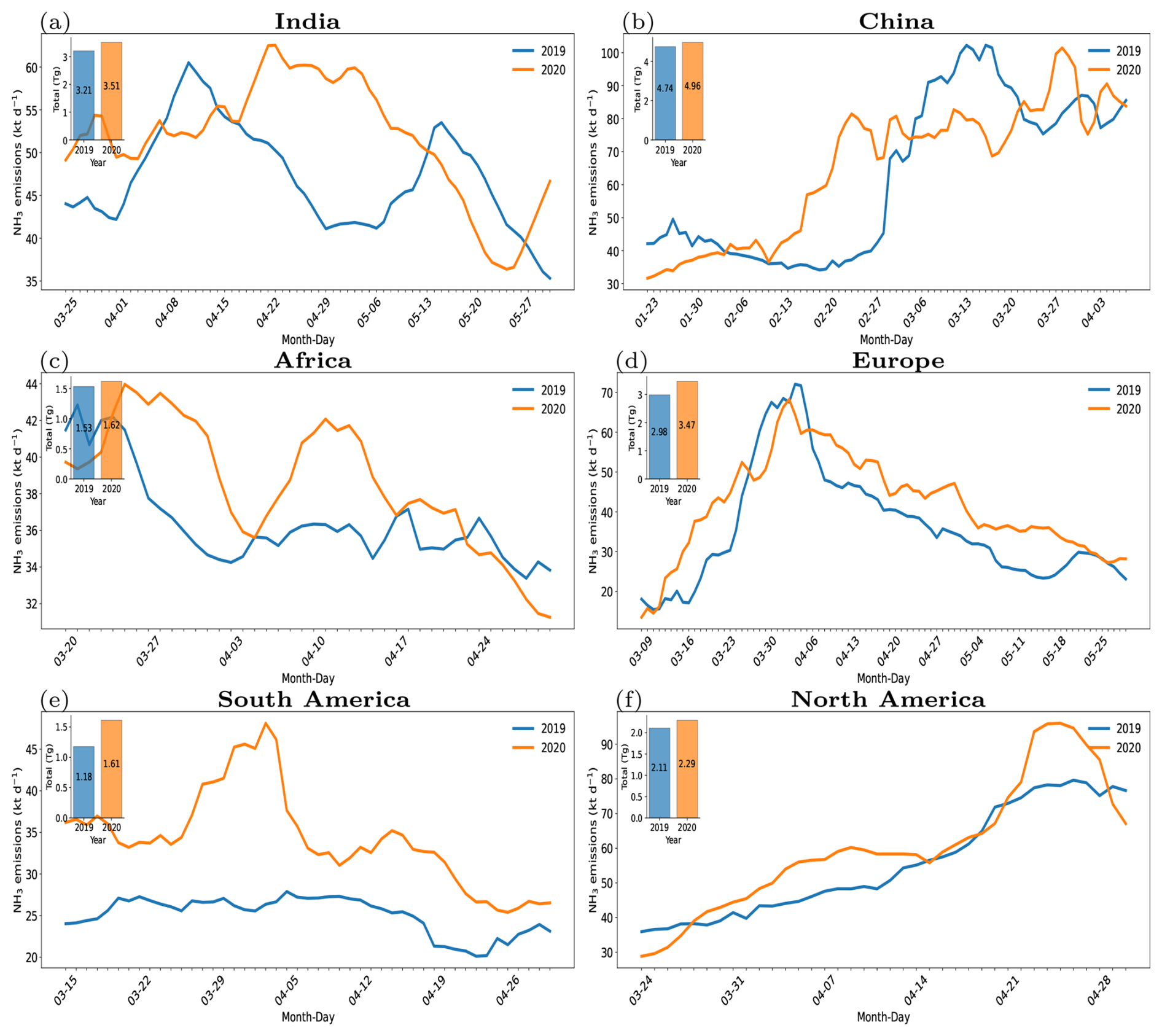
Figure 10 The time series of estimated daily (at 10 d scale) NH₃ emissions and total emissions (bar plots) during the COVID-19 lockdown periods in the year 2020 and pre-COVID year 2019 over different regions across the world.

From our atmospheric inversions, we observe that the annual NH₃ emissions worldwide and across all the selected six regions in the COVID-19 lockdowns in the year 2020 are higher compared to those in the pre-COVID year 2019 (Figs. 6 and 9). Lockdown periods varied across different regions, countries, and cities. However, following the first lockdown in China in the second-to-last week of January 2020, the majority of the first major lockdowns worldwide were implemented between March and May during that year. We defined the lockdown periods in 2020 using the most consistent common dates that aligned with the major lockdowns in each region. Figure 10 compares the estimated daily NH₃ emissions time series and total NH₃ emissions during the COVID-19 lockdown periods in 2020 with the estimated NH₃ emissions during the corresponding period in pre-COVID year 2019 across six regions. Daily (at 10 d scale) variation of the NH₃ emissions during the lockdown periods in 2020 is mostly higher compared to that in the same period in 2019 (Fig. 10). The total NH₃ emissions across these regions in 2020 during the lockdown periods increased by a minimum of ∼5 % (in China) to a maximum of ∼37 % (in South America) compared to the total emissions in this period in 2019 (Fig. 10). The total NH₃ emissions during the lockdown periods in 2020 compared to 2019 across India, Africa, North America, and Europe increased by ∼10 %, ∼6 %, ∼9 %, and ∼16 %, respectively.

The increase in NH₃ emissions from our global inversions during the COVID-19 lockdown periods in 2020 across different regions, compared to the pre-COVID year 2019, raises uncertainty about whether this rise is due to an increase in NH₃ emission sources, due to the impact of meteorology on NH₃ volatilization, or due to a decrease in the atmospheric sink of NH₃ due to the decline in NO_x and SO₂ emissions and concentrations during the lockdowns. However, an increase in NH₃ emission sources during these short lockdown periods seems unlikely, as agricultural practices, the primary source of NH₃ emissions, remained largely unchanged during the lockdowns. This suggests that the observed rise may be more attributable to changes in atmospheric chemistry or to the impact of meteorology on NH₃ volatilization and to the reduction of other species, like SO₂ and NO_x emissions, during the lockdowns (Evangeliou et al., 2025). The single species inversion system used in this study has a limitation and a source of uncertainty to explain this rise in NH₃ emissions. These changes require studying the atmospheric chemistry of ammonia in response to variations in NO_x and SO₂ levels in the atmosphere. A combined multi-species inversion of NO_x, SO₂, and NH₃ emissions would offer valuable insights into the complex chemical interactions among these air pollutant species in the atmosphere.

4.3 Uncertainties and limitations of the present study

There are several uncertainties and limitations associated with our global daily (at 10 d scale) inversion of the anthropogenic NH₃ emissions using IASI NH₃ observations. Although our estimates are mostly consistent and within the range of other recent inversion emissions, our inversion approach and estimates are subject to several uncertainties and limitations. The inversion approach is directly impacted by the errors associated with the observations from the satellite NH₃ retrievals and from model simulations, and it does not provide the uncertainty in emission estimates. A few studies (Cooper et al., 2017; Koukouli et al., 2018) provided some information about the uncertainties in their estimates of other short-lived species like NO_x or SO₂ using the basic or FDMB inversion approach, propagating the observation errors. Although their estimates of uncertainties do not provide the full uncertainty budget, as they do not account for uncertainties associated with model errors or the specific modeling approach, implementing a similar approach could be considered in the future to provide some indication of the uncertainties in our inversion estimates. Systematic errors in satellite retrievals, particularly notable at higher latitudes and during wintertime, may introduce inconsistencies or lead to an overestimation of emissions. Statistical inverse modeling methods (Cao et al., 2020, 2022) account for retrieval errors, but this work is generally focused on the random local and instant noise on the retrievals, and these methods are also highly impacted by systematic errors (Cao et al., 2020, 2022).

The FDMB inversion approach employs a linear sensitivity function based on the perturbations of NH₃ emissions in LMDZ-INCA model simulations, which may oversimplify the complex chemical interactions between air pollutants, including NH₃, in the atmosphere. However, in order to test the impact on the inversion results of the selection of the level of perturbations, we have also conducted a sensitivity analysis with a LMDZ-INCA model simulation using a smaller 20 % perturbation to the prior CEDS anthropogenic NH₃ emissions for the year 2019, in contrast to the original 40 % perturbation used in our FDMB inversion setup. The results show that the differences in the resulting budget of the estimated NH₃ emissions over 2019 and the globe with the application of the FDMB based on these two levels of perturbations are less than 2 %, indicating that the inversion results are not highly sensitive to the choice of perturbation magnitude within this range. As β is the only variable that changes when changing the level of perturbation, this less than 2 % change in the emission estimates necessarily stems from the changes in β due to the reduced prior NH₃ emission perturbations. The good fit between the model simulations with the inverted NH₃ emissions and the IASI NH₃ observations (Sect. 3.2) further strengthens the confidence in the linearization of the inversion problem based on 40 % perturbations to the prior estimate of the emissions. This sensitivity behavior is similar to that of previous applications of the FDMB method to the inversions of anthropogenic NO_x emissions, where different perturbation levels (e.g., 5 %–50 %) to the prior emissions resulted in minimal changes in the posterior anthropogenic NO_x emission estimates at global and regional scales (Cooper et al., 2017; Lamsal et al., 2011; Zheng et al., 2020). The use of a 40 % perturbation in our NH₃ study was motivated by the relatively high uncertainty in the current NH₃ emission inventories, particularly over regions with strong agricultural sources. Nevertheless, our sensitivity test indicates that this choice (at least within a range of 20 %–40 %) is not a critical parameter of our inversions.

Due to the sparseness of daily satellite observations of NH₃ total columns, when the number of high-quality observations within a grid cell is limited, it amplifies uncertainty in the averaged gridded dataset used in the inversions. Consequently, this may lead to an increase in uncertainty in the estimates of daily (at 10 d scale) emissions. As we focus on the inversion of dominated anthropogenic NH₃ emissions, exclusion of the emissions from other sectors like natural sources is a big challenge. This complexity is particularly pronounced in regions dominated by biomass burning NH₃ emissions from wildfires. The local mass-balance inversion approach does not incorporate the transport of ammonia from the non-local biomass burning emissions regions to the local anthropogenic grids, which may lead to an overestimation of the anthropogenic NH₃ emissions in some regions like South America, North America, and Africa. Furthermore, the conservative gap-filling approach employed in this study may introduce some biases and contribute to uncertainties in the final emission estimates.

Although the local finite difference mass-balance approach applied for the inversion of short-lived species like NH₃ in this study, which has a typical short atmospheric lifetime of a few hours to a day, is suitable for inversions at a coarse resolution (∼2°) (Cooper et al., 2017), the typical length scale of our model's spatial resolution (1.27° × 2.5°) can often be reached by the advection of NH₃ within its lifetime. The transport to neighboring grids can lead to a spatial “smearing” effect, where emissions are dispersed away from their source grid cell, introducing errors in mass-balance inversion approaches (Cooper et al., 2017; Li et al., 2019). This problem of spatial smearing in mass-balance inversion approaches is well-documented for short-lived species like NO_x or NH₃ (Cooper et al., 2017; Li et al., 2019). Such smearing can lead, on average, to the underestimation of the regional-scale emissions, as the approach overlooks the fact that the amplitude of the NH₃ signal associated with a given area source decreases with the advection downwind (Cooper et al., 2017; Li et al., 2019). For short-lived species like NO_x, some approaches such as smoothing kernels or iterative FDMB inversion approaches have been used to reduce these errors, but the latter is computationally intensive, especially for global inversions. An iterative FDMB approach (Cooper et al., 2017; Li et al., 2019) can be explored in the future to provide better accuracy in the estimates of NH₃ emissions at a feasible computational cost to overcome this limitation.

In our LMDZ-INCA model setup and inversion framework, the CEDS inventory emissions are regridded to match the model resolution. While this inevitably misses some fine-scale features, our study focuses on the broader regional patterns of NH₃ emissions rather than point-source inversions. The inversions at higher resolution, based on high-resolution regional inventories (e.g., MEIC, NEI, and CAMS-REG) and high-resolution chemistry transport model simulations can bring more robust information of the more localized NH₃ sources such as point sources at sub-national scales. However, the above-mentioned limitation, i.e., the spatial smearing effect (ignoring the advection across the chemistry transport model grid cells) of the FDMB inversion approach, would be exacerbated at such a higher resolution. Even if an iterative FDMB approach is used to overcome this smearing effect at finer resolutions, errors in the derived emission estimates can be amplified (Li et al., 2019). Therefore, application of such an inversion approach at the finer resolution may have limitations in accurately estimating the NH₃ emissions.

Note that an inverse modeling framework including observations of the full reduced nitrogen family (NH${}_x={\mathrm{NH}}_{\mathrm{3}}+{\mathrm{NH}}_{\mathrm{4}}^{+}$) and relying on tests of sensitivities of NH₃ and NH${}_{\mathrm{4}}^{+}$ to changes in NH₃ emissions could provide a more comprehensive constraint on NH₃ emissions, given the rapid gas-particle partitioning of NH₃ to NH${}_{\mathrm{4}}^{+}$ under typical atmospheric conditions. However, current satellite retrievals such as those from IASI and CrIS are primarily focused on gaseous NH₃. The current spaceborne instruments have a limited capability to detect particulate-phase NH${}_{\mathrm{4}}^{+}$. As a result, the observational constraints in our inversion framework are based only on NH₃ columns. Nevertheless, the LMDZ-INCA aerosols–chemistry transport model used in our inversion framework fully represents these chemical conversions of NH₃ to NH${}_{\mathrm{4}}^{+}$ and the partitioning and deposition processes affecting the entire NH_x family. Therefore, the LMDZ-INCA model and, implicitly, our inversion framework account for the fate of NH₃ through its interaction with NH${}_{\mathrm{4}}^{+}$ when deriving relationships between the NH₃ emissions and concentrations.

Over some regions like China and India, the rapid changes in SO₂ emissions in recent years impact the NH₃ concentration in the atmosphere significantly and thus emissions (Luo et al., 2022). Similarly, changes in NO_x emissions and concentration in the atmosphere across different regions alter the formation of ammonium nitrate from ambient ammonia. Therefore, we will investigate the potential of simultaneously assimilating NH₃, SO₂, and NO_x satellite observations to constrain the NH₃ emissions in future studies.

5 Conclusions

In this study, we present satellite-based atmospheric inversion estimates of the global daily (at 10 d scale) NH₃ emissions for a period of 4 years from 2019 to 2022 at 1.27° × 2.5° horizontal resolution using the new version 4 of the IASI-ANNI-NH3-v4 NH₃ observations and the LMDZ-INCA model simulations. We take advantage of the averaging kernel provided in the IASI-ANNI-NH3-v4 data product to evaluate the LMDZ-INCA model suitability for global inversion of the NH₃ emissions. The LMDZ-INCA model-simulated NH₃ total columns using the prior NH₃ emissions are underestimated from the IASI NH₃ observations over most of the selected regions, except over the Indian region, and over a region in Eastern Siberia, where the model shows an overall overestimation from the observations. The simulated NH₃ columns from the LMDZ-INCA model followed the seasonality of the IASI observations over the South American and North American regions and, to some extent, over the European region. However, the seasonal variations over the Indian, Chinese, and African regions are inadequately represented in the model simulations compared to the IASI NH₃ observations.

We use a simple finite difference mass-balance approach for the inversion of global daily (at 10 d scale) NH₃ emissions using the LMDZ-INCA and IASI NH₃ total NH₃ columns that uses a sensitivity parameter of NH₃ columns to changes in the local NH₃ emissions to address non-linear chemistry effects from the model simulations. By conducting an evaluation simulation with the LMDZ-INCA model using IASI-constrained NH₃ emission estimates derived from our global atmospheric inversions for the year 2019, we demonstrate that the substantial improvements in model agreement with the IASI NH₃ observations compared to those using prior NH₃ emissions, across different spatiotemporal scales, strongly validate the robustness and internal consistency of our inversion framework, despite its simplified linearization approach. Our inversions provided an average of ∼97 (∼94–100) Tg yr⁻¹ global annual NH₃ emissions over a period of 4 years from 2019 to 2022. Our IASI-constrained NH₃ emission estimates are ∼61 % (∼55 %–65 %) higher than the prior CEDS anthropogenic NH₃ emissions used in the inversions. A comparison of our inversion estimates with the two independent global bottom-up inventories CAMS and CAMEO shows that our estimates are ∼1.8 times higher than the CAMS anthropogenic NH₃ emissions and ∼1.4 times higher than CAMEO's combined agricultural and natural soil NH₃ emissions. Our global and regional NH₃ emission estimates over India, China, Africa, Europe, South America, North America, and the Middle East are mostly within the range of other global and regional inversion estimates derived based on the IASI or CrIS satellite NH₃ observations. Our simple inversion framework lacks the ability to attribute contributions from the sectors like biomass burning to the estimates of the anthropogenic NH₃ emissions. Therefore, the estimated NH₃ emissions over some regions like South America and Africa may be overestimated due to predominant biomass burning from wildfires in these regions. Our NH₃ emission estimates over Europe are ∼72 % higher compared to the prior CEDS inventory emissions; however, they are consistent with two recent inversion estimates. We observed an increasing trend of the NH₃ emission over China and Africa and a decreasing trend over the Indian region over a 4-year period from 2019 to 2022. Our estimates of the NH₃ emissions show a strong seasonal variation over most of the selected regions that is currently poorly known or almost absent in bottom-up inventories.

We also analyzed the impact of restrictions during the COVID-19 lockdown periods in 2020 over different regions across the world on the estimated daily (at 10 d scale) NH₃ emissions in comparison to the pre-COVID year 2019. Our inversion estimates show that the total NH₃ emissions across China, India, Africa, North America, Europe, and South American during the lockdown periods in the year 2020 increased by, respectively, ∼ 5 %, ∼10 %, ∼6 %, ∼9 %, ∼16 %, and ∼37 % compared to the total emissions in the same periods in 2019. However, this increase in NH₃ emissions from our global atmospheric inversions during the COVID-19 lockdowns, compared to the pre-COVID year 2019, raises a question about whether this rise is due to an increase in NH₃ emission sources, due to the impact of meteorology on NH₃ volatilization, or due to a decrease in the atmospheric sink of atmospheric NH₃ due to the decline in NO_x and SO₂ emissions and ambient concentrations during the lockdown periods. However, our inversion system fails to explain this rise in NH₃ emissions. Therefore, a more comprehensive inversion approach, integrating NO_x, SO₂, and NH₃ simultaneously, would provide deeper insights into the complex chemical interactions between these pollutants in the atmosphere.