Influence of various criteria on identifying the springtime tropospheric ozone depletion events (ODEs)at Utqiaġvik, Arctic

Tropospheric ozone depletion events (ODEs) occurring in the Arctic spring are a unique photochemical phenomenon in which the boundary layer ozone drops rapidly to near-zero levels. However, the criterion for identifying ODEs remains inconsistent among different studies, which may influence conclusions regarding the characteristics of ODEs. To address this issue, in this study, we applied various criteria used in previous studies to identify springtime ODEs at Utqiaġvik, Arctic (the BRW Station), based on observational data spanning 23 years (2000–2022), and investigated the influence of implementing different criteria. We compared three types of criteria: traditional methods (fixed thresholds), variability-based methods (considering the mean value and standard deviation), and machine learning methods (Isolation Forest), and we found that criteria using fixed thresholds (e.g., 10 ppbv) and relative thresholds based on monthly averaged ozone levels (0.42 times the monthly average) are more suitable for capturing ODEs at BRW compared to other criteria. Results applying these appropriate criteria reveal a significant decline in ODE occurrence frequency over the investigated 23 years, particularly in April, suggesting potential links to climate change and Arctic sea ice melting. However, implementing relative thresholds or more stringent fixed thresholds (5 and 4 ppbv) instead of the 10 ppbv threshold reveals a more significant decline in the number of ODE hours across these 23 years. Further investigation of meteorological conditions indicates that ODEs at BRW are more prevalent under northerly and northeasterly winds with moderate wind speeds (3–6 m s⁻¹), at lower temperatures and higher pressures, while severe ODEs are more associated with lower wind speeds and temperatures below 256 K. This research highlights the importance of selecting appropriate criteria to accurately identify ODEs and contributes to a better understanding of the complex processes driving the Arctic ODEs.

1 Introduction

The Arctic has been described as an important “window” on the global environment, as changes in the Arctic serve as a precursor to global changes anticipated as the Earth's temperature rises (Thoman et al., 2023). Among all the changes in the Arctic environment, the variation in the ozone concentration during the spring season has attracted considerable attention from the scientific community. In the stratosphere, the depletion of ozone in the Arctic spring, which is caused by the existence of polar stratospheric clouds and halogen compounds (Crutzen and Arnold, 1986; Cairo and Colavitto, 2020; Seinfeld and Pandis, 2006; Akimoto, 2016), allows increased UV radiation that can lead to higher rates of skin cancer, cataracts, and weakened immune systems in humans (Umar and Tasduq, 2022), while also affecting marine and terrestrial ecosystems, potentially altering weather patterns and contributing to climate change (Liu et al., 2022).

In contrast to stratospheric ozone depletion, in the lower troposphere, a unique phenomenon, namely ozone depletion events (ODEs), has also been frequently observed in the near-surface layer of the Arctic since the 1980s (Oltmans, 1981; Barrie et al., 1988; Bottenheim et al., 1986, 2002; Anlauf et al., 1994; Shupe et al., 2022). This phenomenon is associated with a photochemical process that can activate halogen ions (i.e., Br⁻, Cl⁻, I⁻) from substrates such as ice/snow packs (Lehrer et al., 2004; Simpson et al., 2007b; Abbatt et al., 2012; Pratt et al., 2013; Custard et al., 2017) and sea-salt aerosols (Michalowski et al., 2000; Yang et al., 2010, 2019, 2020; Thomas et al., 2011, 2012; Huang et al., 2020) into reactive halogens that can deplete ozone. Consequently, the ozone in the polar boundary layer frequently falls from background levels (30–40 ppbv) to less than 10 ppbv or even near-zero values within a few days or even hours in the springtime of the Arctic.

The occurrence of ODEs is related to a complex photochemical process as follows (Simpson et al., 2007b):

$$\begin{array}{}\text{(R1)}& \begin{array}{rl}& {\mathrm{X}}_{\mathrm{2}}+h\mathit{\nu }\to \mathrm{2}\mathrm{X},\\ & \mathrm{2}\mathrm{X}+\mathrm{2}{\mathrm{O}}_{\mathrm{3}}\to \mathrm{2}\mathrm{XO}+\mathrm{2}{\mathrm{O}}_{\mathrm{2}},\\ & \underset{\mathrm{¯}}{\mathrm{XO}+\mathrm{XO}\to {\mathrm{X}}_{\mathrm{2}}\left(\mathrm{2}\mathrm{X}\right)+{\mathrm{O}}_{\mathrm{2}},}\\ & \text{Net}:\mathrm{2}{\mathrm{O}}_{\mathrm{3}}+h\mathit{\nu }\to \mathrm{3}{\mathrm{O}}_{\mathrm{2}}.\end{array}\end{array}$$

In the reaction cycle (Reaction R1), X denotes halogen species (i.e., Br, Cl, and I). When the sun rises in the Arctic spring, halogen-containing compounds (i.e., X₂) in the atmosphere are photodissociated into halogen atoms (i.e., X). These halogen atoms subsequently react rapidly with ozone, producing halogen monoxide XO, as depicted in Reaction (R1). XO then participates in self-reactions that regenerate X atoms, thereby depleting ozone without consuming halogens.

However, in the reaction cycle (Reaction R1), the total amount of halogens remains constant, which is inconsistent with measurements at Arctic coastal stations, where a substantial increase in halogen concentrations is observed during ODEs (Hausmann and Platt, 1994; Zhao et al., 2016). Furthermore, previous research has demonstrated that ozone cannot be depleted in such a short time if only gas-phase reactions occur (Lehrer et al., 2004). Thus, another reaction cycle, including heterogeneous reactions, was proposed to explain the rapid ozone decline and the large amount of reactive halogens in the atmosphere during ODEs (Fan and Jacob, 1992; McConnell et al., 1992; Platt and Lehrer, 1997; Tang and McConnell, 1996; Wennberg, 1999). Using bromine as a representation of halogen species, this proposed reaction cycle can be outlined as follows:

$$\begin{array}{}\text{(R2)}& \begin{array}{rl}& \mathrm{BrO}+{\mathrm{HO}}_{\mathrm{2}}\to \mathrm{HOBr}+{\mathrm{O}}_{\mathrm{2}},\\ & \mathrm{HOBr}+{\mathrm{H}}^{+}+{\mathrm{Br}}^{-}\stackrel{\mathrm{mp}}{\to }{\mathrm{Br}}_{\mathrm{2}}+{\mathrm{H}}_{\mathrm{2}}\mathrm{O},\\ & {\mathrm{Br}}_{\mathrm{2}}+h\mathit{\nu }\to \mathrm{2}\mathrm{Br},\\ & \underset{\mathrm{¯}}{\mathrm{Br}+{\mathrm{O}}_{\mathrm{3}}\to \mathrm{BrO}+{\mathrm{O}}_{\mathrm{2}},}\\ & \mathrm{\text{Net:}}{\mathrm{O}}_{\mathrm{3}}+{\mathrm{HO}}_{\mathrm{2}}+{\mathrm{H}}^{+}+{\mathrm{Br}}^{-}+h\mathit{\nu }\stackrel{\mathrm{mp}}{\to }\mathrm{2}{\mathrm{O}}_{\mathrm{2}}+\mathrm{Br}+{\mathrm{H}}_{\mathrm{2}}\mathrm{O}.\end{array}\end{array}$$

In the reaction cycle (Reaction R2), hypobromous acid (HOBr) can activate bromides (Br⁻) from substrates such as snowpacks on the sea ice and sea-salt aerosols, leading to the conversion of bromides into reactive halogen species such as Br₂, which in turn undergo photodissociation and consume ozone. Consequently, ozone is continuously depleted, and the total bromine concentration in the atmosphere is explosively elevated during ODEs. Thus, this process is referred to as the “bromine explosion mechanism” (Platt and Lehrer, 1997; Wennberg, 1999).

The occurrence of ODEs is predominantly confined to the spring season due to the unique combination of meteorological and chemical conditions (Lehrer et al., 2004). First, the sunlight during spring is essential for photochemical reactions to take place, which are crucial for converting inert halogen ions into reactive halogens. Second, the strong temperature inversion that forms in the spring effectively isolates the boundary layer air from the free troposphere, preventing the downward mixing of ozone-rich air from aloft and allowing the reactive halogens to efficiently deplete the local ozone. Additionally, the snowpack above the sea ice in springtime acts as a significant source of halogen ions, as the brine layer on the sea ice is enriched with halogens that can be released into the atmosphere through photochemical processes. These factors collectively create the ideal conditions for ODEs to occur in the spring, while such conditions are not simultaneously met in other seasons.

ODEs can exert a profound influence on both the Arctic environment and global ecosystems. First, they can alter the radiation balance in the Arctic by reducing the infrared radiation absorbed by the atmosphere (Lacis et al., 1990). Moreover, during ODEs, the oxidative capacity of the Arctic atmosphere is dominated by enhanced bromine compounds. This shift in the oxidative capacity facilitates the oxidation of elemental mercury (Hg(0)), followed by the deposition of active mercury (Hg(II)), a pollutant that is highly toxic to humans. The increased deposition of active mercury ultimately jeopardizes human health in mid-latitude regions through snow melting and oceanic circulations (Ariya et al., 2004; Pratt et al., 2013; Dastoor et al., 2022; Basu et al., 2022).

Since the discovery of ODEs, our understanding of this phenomenon has improved, such as the role of sea ice formation (Jones et al., 2011; Lehrer et al., 2004; Simpson et al., 2007a; Abbatt et al., 2012; Peterson et al., 2019), the linkage to climate variability (Koo et al., 2014), the influence of snowpack photochemical emissions (Pratt et al., 2013; Custard et al., 2017; Herrmann et al., 2021, 2022), and Arctic blowing snow (Chen et al., 2022; Yang et al., 2010, 2019, 2020; Huang et al., 2020), as well as the connection to the total column ozone (Cao et al., 2022). However, to date, the criterion for identifying ODEs remains unclear. In previous studies, the occurrence of ODEs was mostly recognized by the volume mixing ratio of the surface ozone when the surface ozone decreased to a level below a fixed threshold. However, the threshold is inconsistent across different studies, ranging from 20 down to 4 ppbv. For example, Tarasick and Bottenheim (2002) and Koo et al. (2012) used a threshold of 10 ppbv, while Bottenheim et al. (2009), Frieß et al. (2011), and Jacobi et al. (2010) utilized 5 ppbv. Meanwhile, Piot and Von Glasow (2008) and Ridley et al. (2003) identified ODEs using a more stringent 4 ppbv threshold. In contrast to these studies employing a fixed threshold, Cao et al. (2022) used a criterion depending on the mean value and the standard deviation of the surface ozone across various months and years to identify ODEs. This criterion was based on the method of Bian et al. (2018), which was originally used to indicate uncommon variations in the surface ozone in polar regions. In that study, Cao et al. (2022) applied this criterion to pick out ODE hours from surface ozone measurements at the Halley Station in Antarctica for the spring months from 2007 to 2013, and the results demonstrated that the criterion was effective in identifying ODEs from the springtime surface ozone measurements at the Halley Station.

Because the identification criterion for ODEs may influence conclusions regarding the characteristics of ODEs, such as the interannual variability of ODEs, the relationship between meteorological conditions, and the occurrence frequency of ODEs, in this study, we employed various criteria to identify ODEs from 23 years of spring observational data detected at Utqiaġvik in Alaska and explored the impacts of using different screening criteria on the results. We then selected appropriate criteria to investigate the correlations between meteorological parameters (e.g., wind speed, wind direction, temperature, and pressure) and the occurrence of ODEs and compared the results to assess the impact of different criteria on the conclusions.

2 Observational data and screening criteria

We first used different criteria to screen out ODE hours from observational data for the springtime across 23 years (2000–2022). Then, based on a comparison of the screening results, we investigated the properties of these ODE screening criteria.

2.1 Observational data

Surface ozone mixing ratio and meteorological parameters (pressure, 2 m temperature, 10 m wind speed and direction) at Utqiaġvik (the BRW Station; see Fig. 1 for the geographic location) were taken from the National Oceanic and Atmospheric Administration/Oceanic and Atmospheric Research/Global Monitoring Laboratory (NOAA/OAR/GML) baseline observatory (https://gml.noaa.gov/aftp/data/ozwv/SurfaceOzone/Version_1/BRW/, last access: 26 September 2025) (McClure-Begley et al., 2024; Crocker, 2024), which are freely provided to the public and scientific community. We adopted the data for the years 2000–2022 with a 1 h time resolution and focused only on the three months of spring (March, April, and May) in the present study.

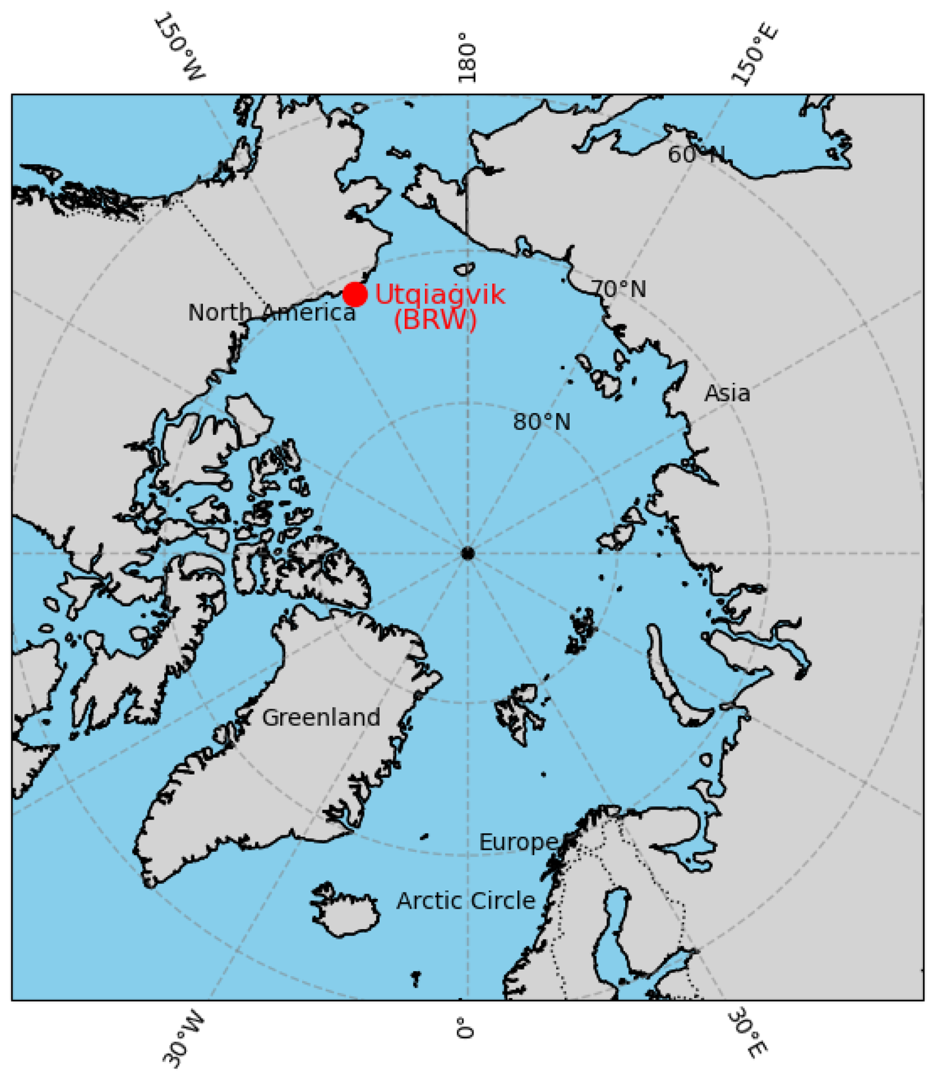
Figure 1 Location of the BRW Station in the Arctic.

2.2 Criteria for identifying ODEs

Three types of criteria (traditional methods, variability-based methods, and machine learning methods) were used to screen out ODE hours from the measurements, which are listed in Table 1 and described in detail below.

Table 1 Criteria used to identify ODEs in this study and their expressions.

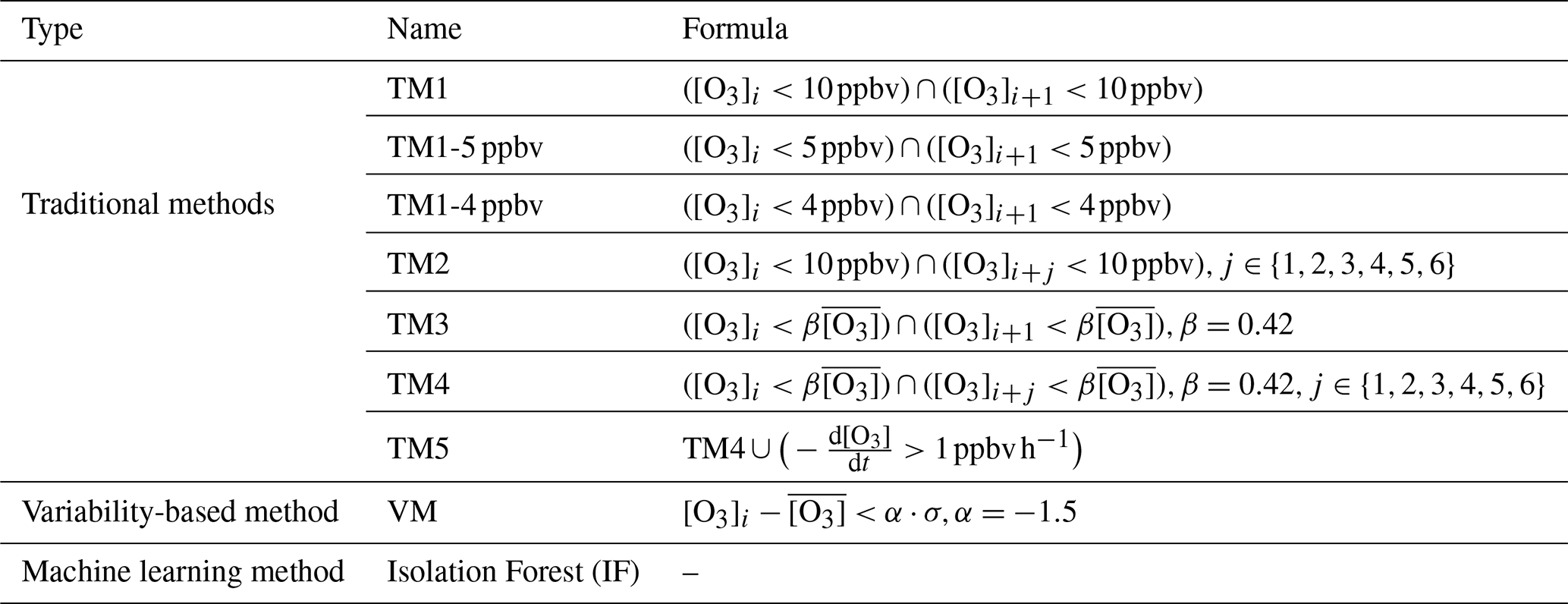
2.2.1 Traditional methods

This kind of method defines ODEs according to the mixing ratios of ozone. The first criterion to be tested is similar to that used by Halfacre et al. (2014), in which ODEs are defined as time periods when the ozone mixing ratio falls below 10 ppbv. Moreover, the situation with an ozone value lower than 10 ppbv should last for longer than 1 h (i.e., [O₃]<10 ppbv at two consecutive time points). Thus, this criterion can be described as follows:

$$\begin{array}{}\text{(1)}& \left(\right[{\mathrm{O}}_{\mathrm{3}}{]}_i<\mathrm{10})\cap ([{\mathrm{O}}_{\mathrm{3}}{]}_{i+\mathrm{1}}<\mathrm{10}),\end{array}$$

in which [O₃]_i is the ozone mixing ratio at the ith time point. This criterion is referred to as TM1 in the following context (see Table 1). In previous studies (Bottenheim et al., 2009; Frieß et al., 2011; Jacobi et al., 2010; Piot and Von Glasow, 2008; Ridley et al., 2003), different constant thresholds (e.g., 5 and 4 ppbv) have also been utilized for identifying ODEs. Therefore, in addition to the commonly used 10 ppbv threshold, we also tested 5 and 4 ppbv thresholds in this study and named them TM1-5 ppbv and TM1-4 ppbv (see Table 1).

We then modified TM1 to obtain different screening criteria. First, we relaxed the duration of ODEs in the TM1 criterion. Instead of using a consecutive 2 h duration, we defined ODEs as the initial hour when ozone is lower than 10 ppbv, if this hour is followed by at least one other hour with ozone below 10 ppbv within the next 6 h (see TM2 in Table 1):

$$\begin{array}{}\text{(2)}& \left(\right[{\mathrm{O}}_{\mathrm{3}}{]}_i<\mathrm{10})\cap ([{\mathrm{O}}_{\mathrm{3}}{]}_{i+j}<\mathrm{10}),j\in \mathit{\{}\mathrm{1},\mathrm{2},\mathrm{3},\mathrm{4},\mathrm{5},\mathrm{6}\mathit{\}}.\end{array}$$

This criterion can include time periods when an abrupt increase in ozone occurs during ODEs due to processes such as stratospheric intrusion and local anthropogenic emissions.

We also replaced the fixed value (10 ppbv) used in TM1 with a percentage of the monthly averaged ozone value (see Fig. 2, showing the monthly averaged ozone mixing ratios in different months and years), and named this criterion TM3:

$$\begin{array}{}\text{(3)}& \left(\right[{\mathrm{O}}_{\mathrm{3}}{]}_i<\mathit{\beta }\stackrel{\mathrm{‾}}{\left[{\mathrm{O}}_{\mathrm{3}}\right]})\cap ([{\mathrm{O}}_{\mathrm{3}}{]}_{i+\mathrm{1}}<\mathit{\beta }\stackrel{\mathrm{‾}}{\left[{\mathrm{O}}_{\mathrm{3}}\right]}).\end{array}$$

In Eq. (3), $\stackrel{\mathrm{‾}}{\left[{\mathrm{O}}_{\mathrm{3}}\right]}$ is the averaged ozone value of the corresponding month, and β is a constant that is artificially given. For a better comparison, we determined the coefficient β to be 0.42 using the least squares method, so that $\mathit{\beta }\stackrel{\mathrm{‾}}{\left[{\mathrm{O}}_{\mathrm{3}}\right]}$ in Eq. (3) is closest to the constant 10 ppbv used in TM1 (see Fig. S1 in the Supplement for the comparison between $\mathit{\beta }\stackrel{\mathrm{‾}}{\left[{\mathrm{O}}_{\mathrm{3}}\right]}$ and the 10 ppbv constant).

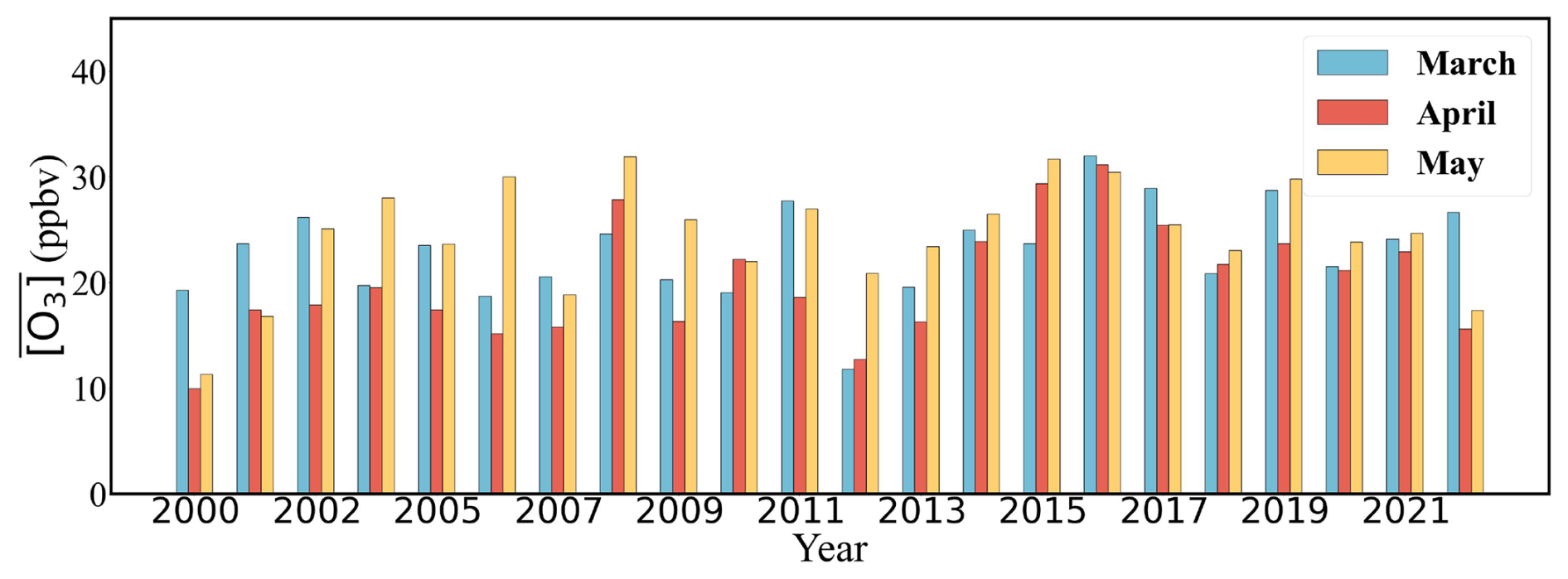
Figure 2 Monthly averaged ozone mixing ratios at the BRW Station for spring months (March, April, and May) from 2000 to 2022.

After that, by integrating TM2 and TM3, we obtained TM4 (see Table 1):

$$\begin{array}{}\text{(4)}& \left(\right[{\mathrm{O}}_{\mathrm{3}}{]}_i<\mathit{\beta }\stackrel{\mathrm{‾}}{\left[{\mathrm{O}}_{\mathrm{3}}\right]})\cap ([{\mathrm{O}}_{\mathrm{3}}{]}_{i+j}<\mathit{\beta }\stackrel{\mathrm{‾}}{\left[{\mathrm{O}}_{\mathrm{3}}\right]}),j\in \mathit{\{}\mathrm{1},\mathrm{2},\mathrm{3},\mathrm{4},\mathrm{5},\mathrm{6}\mathit{\}}.\end{array}$$

Based on TM4, we further took the depleting stage of ozone into consideration. Typically, a complete ODE can be divided into three stages. The first stage is the start of the ODE, when the ozone depletes very fast. The second stage is when the ozone remains at a low level (e.g., <10 ppbv), which is the maintenance of the ODE. The third stage is when the ozone returns to background levels, which is the termination of the ODE. The TM4 criterion described above basically accounts for time periods corresponding to the second stage. In the next criterion, in addition to time points that are identified by TM4, time points when the depletion rate of ozone is larger than 1 ppbv h⁻¹ were also added:

$$\begin{array}{}\text{(5)}& \text{TM4}\cup \left(-{\displaystyle \frac{\mathrm{d}\left[{\mathrm{O}}_{\mathrm{3}}\right]}{\mathrm{d}t}}>\mathrm{1}\mathrm{ppbv}{\mathrm{h}}^{-\mathrm{1}}\right).\end{array}$$

This criterion further considers time periods representing the first stage of the ODE, and is referred to as TM5, which is listed in Table 1.

2.2.2 Variability-based method

In our previous work (Cao et al., 2022), we picked out time points representing the tropospheric ODEs at the Halley Station in Antarctica according to the variability in the surface ozone mixing ratio, which included considerations of both the mean value and the standard deviation. This method for identifying ODEs was proposed based on the study of Bian et al. (2018), where the ozone mixing ratio fulfills the following criterion:

$$\begin{array}{}\text{(6)}& [{\mathrm{O}}_{\mathrm{3}}{]}_i-\stackrel{\mathrm{‾}}{\left[{\mathrm{O}}_{\mathrm{3}}\right]}<\mathit{\alpha }\cdot \mathit{\sigma },\end{array}$$

in which [O₃]_i is the ozone mixing ratio at the ith time point, and $\stackrel{\mathrm{‾}}{\left[{\mathrm{O}}_{\mathrm{3}}\right]}$ is the monthly averaged ozone value. σ in Eq. (6) denotes the standard deviation. α is a constant that was set to −1.5 in that study (Cao et al., 2022) so that many partial ODEs (i.e., $\mathrm{10}\mathrm{ppbv}<\left[{\mathrm{O}}_{\mathrm{3}}\right]<\mathrm{20}\mathrm{ppbv}$) can also be identified. According to the criterion described by Eq. (6), ODEs were defined as the time periods when the surface ozone drops to an uncommonly low level, rather than the time periods when the surface ozone falls below a specific threshold, and we named this criterion VM in the following context (see Table 1).

2.2.3 Machine learning method

Recently, machine learning methods have been used to investigate ODEs and the associated variability in tropospheric BrO in the Arctic (Bougoudis et al., 2022). In this study, a machine learning method, Isolation Forest (Liu et al., 2008; Al Farizi et al., 2021), which can detect anomalies in data, was used to screen out ODE hours from the measurements (i.e., IF in Table 1). The Isolation Forest method is a commonly used machine learning approach for detecting anomalies in data, based on decision tree algorithms. In this method, anomalies are detected by constructing an ensemble of isolation trees, where each tree recursively isolates data points by randomly selecting split values until each point is isolated. After that, the average path length for each point across all trees is calculated to derive an average anomaly score, with higher scores indicating a greater likelihood of being an anomaly. Values of parameters utilized in this method for the current study are outlined as follows: n_estimators (number of trees), 100; max_samples (number of samples), auto (i.e., using all samples); contamination (proportion of outliers), auto (i.e., auto-selected based on data arrangement); max_features (maximum number of features), 1.0 (i.e., using all features).

2.3 Regression of ODE hours over time

We employed linear regression analysis (Draper and Smith, 1998; Weisberg, 2005; Montgomery et al., 2021) to assess the trend of ODE occurrence over time. Linear regression is a classical statistical method that is widely used to quantify the trend of a dependent variable with respect to one or more independent variables through the method of least squares. The form of the linear regression used in this study is

$$\begin{array}{}\text{(7)}& Y=a(X-\mathrm{2000})+b,\end{array}$$

where Y is the dependent variable (annual ODE hours in this study), and X is the independent variable (year in this study). The slope a is the regression coefficient, representing the rate of change of Y with X−2000. The intercept b represents the value of Y when $X-\mathrm{2000}=\mathrm{0}$.

To evaluate the significance of the regression, we also calculated the p value. The p value is usually used to judge whether the regression is significant or not. Specifically, a p value less than 0.05 (p<0.05) suggests that there is less than a 5 % probability that the observed trend could have occurred by random chance, indicating a significant trend. A p value less than 0.01 (p<0.01) suggests that there is less than a 1 % probability, indicating a highly significant trend. In contrast, $\mathrm{0.05}<p\le \mathrm{0.1}$ indicates a close to significant trend, and p>0.1 denotes an insignificant trend.

3 Results and discussions

In this section, we first show the identification results of ODE hours after applying various criteria. These results were also compared and discussed to examine the characteristics and performance of each criterion. Subsequently, we selected several appropriate criteria for a detailed comparative analysis. This comparative examination allowed us to elucidate the effects of using different criteria on the interannual variability of ODEs and their associations with meteorological parameters.

3.1 Interannual variability of ODE hours screened using various criteria

Figure 3 depicts the annual changes in ODE hours identified by various criteria across the 2000–2022 period, reflecting the characteristics of each screening criterion. We first focus on the results obtained by the traditional methods (i.e., TM1–TM5; see Fig. 3a). Generally, the results derived from all the traditional methods display a similar pattern, and a general decline in ODE occurrence over this 23-year period can be observed. The years with the most ODE hours were found to be between 2000 and 2012. Between 2000 and 2012, the ODE hours exhibit a pattern of fluctuation throughout this period. There appears to be a weak upward trend between 2000 and 2012 if the year 2000 is excluded, suggesting a slight increase in ODE hours during this time period. This result is consistent with that of Oltmans et al. (2012), which reported an increase in the ODE occurrence frequency in the time period of 1973–2010. However, after 2012, the curves of all TM methods show a sharp decline, indicating a strong decrease in ODE hours in recent years. This finding is in accordance with the results of Law et al. (2023), which found a pronounced increasing trend in the tropospheric ozone at BRW in the springtime of the period 1999–2019.

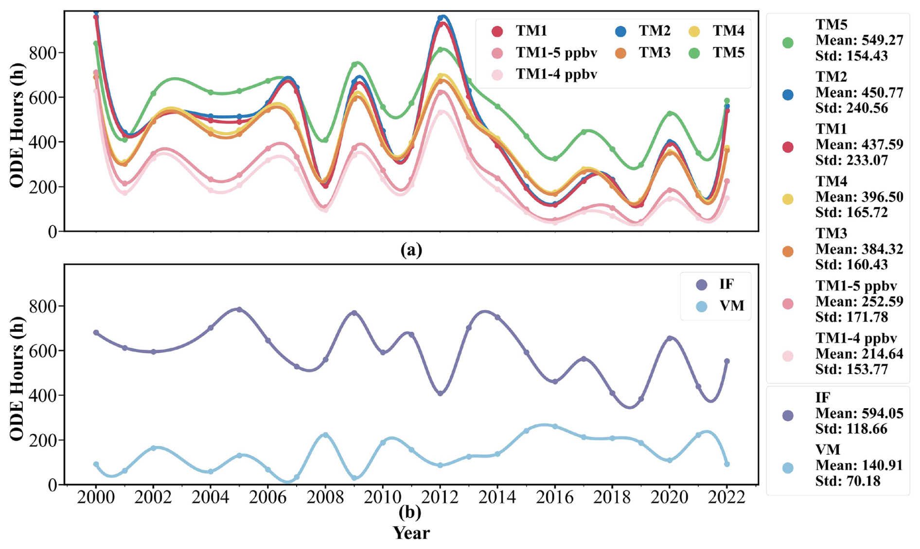
Figure 3 Number of ODE hours identified by (a) traditional methods (TM1–TM5), (b) the variability-based method (VM), and the Isolation Forest method (IF) from 2000 to 2022.

With respect to each TM criterion, it can be seen in Fig. 3a that the results using the thresholds of 5 ppbv (TM1-5 ppbv) and 4 ppbv (TM1-4 ppbv) are largely consistent with those using the 10 ppbv threshold (TM1), but with a significant reduction in the number of ODE hours, because more stringent thresholds were applied. The ODE hours identified using the 5 and 4 ppbv thresholds are 46 % and 55 % fewer, respectively, than those identified using the 10 ppbv threshold on average. Figure 3a also shows that the results obtained by TM1 and TM2 are almost identical, indicating that the influence brought about by the modification of the ODE duration (from a continuous 2 h occurrence to a following 1 h occurrence within a 6 h period) is negligible. This also means that during occurrences of ODEs, ozone concentrations rarely make a sudden transition from below 10 to above 10 ppbv. ODEs typically persist for at least 2 h in the majority of cases. Similar behavior was also found between the results obtained by TM3 (ozone below $\mathrm{0.42}\stackrel{\mathrm{‾}}{\left[{\mathrm{O}}_{\mathrm{3}}\right]}$ for continuous 2 h) and TM4 (ozone below $\mathrm{0.42}\stackrel{\mathrm{‾}}{\left[{\mathrm{O}}_{\mathrm{3}}\right]}$ for a start hour and a following hour within a 6 h period). We then focus on the differences between the results obtained by using TM1 and TM3. It is not surprising to see that when the difference between $\mathrm{0.42}\stackrel{\mathrm{‾}}{\left[{\mathrm{O}}_{\mathrm{3}}\right]}$ and 10 ppbv is significant, there is a considerable discrepancy in the screening results. For instance, the discrepancy in the results for the year 2012 is remarkable (see Fig. 3a), because the mean values of ozone in March and April of this year are quite low ($\mathrm{0.42}\stackrel{\mathrm{‾}}{\left[{\mathrm{O}}_{\mathrm{3}}\right]}=\mathrm{4.95}$ and 5.34, respectively); conversely, when the difference is smaller, the discrepancy is less pronounced, such as those for the years 2008 and 2014. As is well known, the background levels of Arctic ozone vary across different years and seasons, driven by factors such as climate change and atmospheric circulation. For instance, the average ozone level in the Arctic in the springtime of 2023 was reported to be abnormally higher than historical levels (Ding et al., 2024). Considering these dramatic changes in the background levels of ozone in the Arctic, using “tailored” thresholds based on average ozone levels across different time periods (i.e., TM3, TM4) might be another appropriate choice to identify ODEs. With respect to TM5 ($\text{TM4}\cup (-\frac{\mathrm{d}\left[{\mathrm{O}}_{\mathrm{3}}\right]}{\mathrm{d}t}>\mathrm{1}\mathrm{ppbv}{\mathrm{h}}^{-\mathrm{1}})$), it is seen in Fig. 3a that the overall trend of the TM5 curve is generally similar to that of TM4, while the TM5 curve is consistently above the TM4 curve by a margin (152 h on average), indicating the additional hours representing ozone-depleting stages considered in the TM5 criterion.

Regarding the variability-based method (i.e., VM in Fig. 3b), its behavior is remarkably different from that of the TM methods. Generally, it screens out the fewest ODE hours, indicating that it is the most rigorous selection criterion compared with the others. Moreover, it is shown in Fig. 3b that between 2000 and 2005, the trend of the VM curve is consistent with that of the TM curves. However, during other time periods, such as 2010–2015, the VM curve displays a trend that contrasts with the patterns observed in the TM curves. This is because the VM criterion, in addition to the mean value, also takes the standard deviation into account. When the ozone concentration oscillates greatly, the standard deviation will be high, thus dominating the criterion given by Eq. (6). As a result, the variability of the criterion is more closely aligned with the patterns of the standard deviation, rather than following the mean ozone value. More discussion is given in the following context.

With respect to the Isolation Forest method (see the IF curve in Fig. 3b), the number of ODE hours screened by this method is generally comparable to those identified using TM methods. Interestingly, after 2014, the IF curve behaves similarly to that of the TM methods, while before 2008, the IF curve's trend resembles that of the VM method's trend, although the values are significantly higher, indicating a possible consideration of the standard deviation in the IF method. Because of the black box characteristics of machine learning models (Hassija et al., 2024), it is difficult for us to further explore the reasons and principles behind the screening results of this method. Further interpretability of this machine learning method is also one of the areas we aim to investigate in the future.

In the subsequent analysis, we will focus on two specific years (2012 and 2021) to investigate more deeply the characteristics of these criteria for identifying ODEs. These two years were selected because 2012 is one of the years with the most ODE hours (530–950 h indicated by the TM methods). In contrast, 2021 is one of the years with the least ODE hours (60–350 h) but has frequent oscillation in ozone levels.

3.2 ODE hours on specific years identified by different criteria

The results of TM1 are almost identical to those of TM2, and the results of TM3 are largely in line with TM4. Additionally, results of TM1–5 ppbv and TM1–4 ppbv show a decrement from TM1's results, and results of TM5 show an increment from TM4's, while maintaining essentially a similar trend. Therefore, in this section, we only compare the results for ODE hours screened by TM1, TM4, VM, and IF methods in specific years (i.e., 2012 and 2021). Results for ODE hours identified using other criteria can be found in Figs. S2 and S3.

3.2.1 Traditional methods

Figures 4a and b illustrate the results of screened ODE hours using the TM1 criterion for the years 2012 and 2021. We found that in the year 2012, because the average ozone level was lower than that in 2021, the identified ODE hours in 2012 (i.e., 925 h) are significantly more than those in 2021 (i.e., 165 h). This implies that when TM1 is applied, the number of identified ODE hours is positively correlated with the annual average ozone concentration for a specific year, which can be easily expected since a year with a lower ozone level is more likely to meet the fixed threshold criteria.

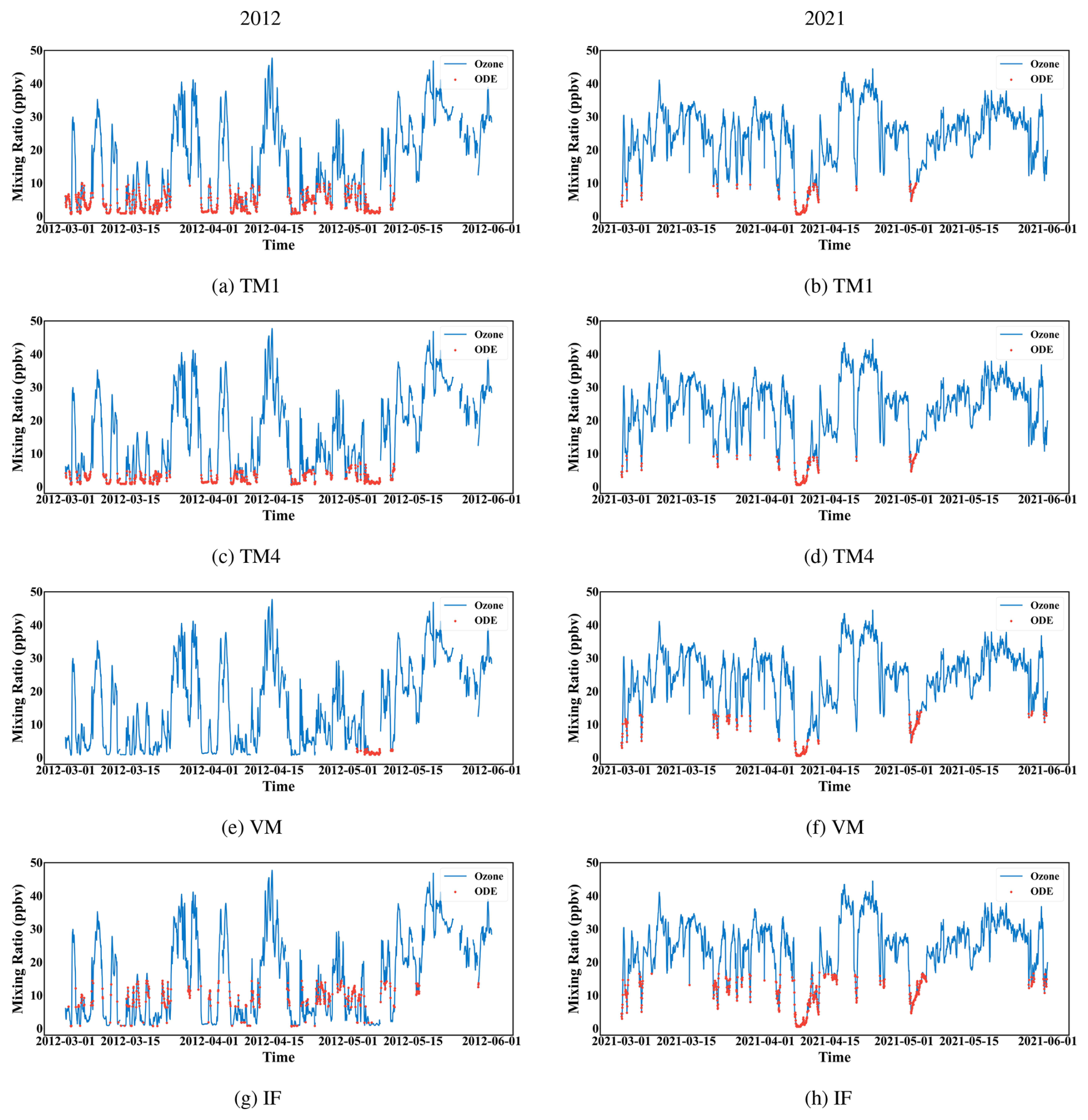
Figure 4 Screened results for 2012 and 2021 using various criteria. The blue curve represents the hourly time series of the ozone mixing ratio, and the red dots denote the ODE hours identified by various criteria.

The TM1 criterion is straightforward and easy to apply. However, Fig. 4b shows that in 2021, many time points when the ozone mixing ratio decreased sharply were not identified as ODE hours because the depletion was not strong enough to reduce the ozone level to below 10 ppbv. This is also the possible reason why another criterion for identifying “partial” ODEs (i.e., $\mathrm{10}\mathrm{ppbv}<\left[{\mathrm{O}}_{\mathrm{3}}\right]<\mathrm{20}\mathrm{ppbv}$) is often suggested in many previous studies (Ridley et al., 2003; Koo et al., 2012; Halfacre et al., 2014).

In contrast to the TM1 method, TM4 gives different thresholds according to the monthly averaged ozone value across different months and years. Generally, the results obtained by TM4 are consistent with those obtained by TM1 (see Fig. 4c and d). In months and years that have low ozone concentrations (<15 ppbv, e.g., year 2012, see Fig. 4c), the implementation of TM4 would exert a more stringent threshold so that fewer ODE hours are identified. In contrast, in months and years that have high ozone concentrations (e.g., year 2021, see Fig. 4d), comparable or more ODE hours can be identified using this criterion.

3.2.2 Variability-based method

As discussed above, the variability-based method screened out significantly fewer ODE hours than the other methods. For instance, in 2012, the VM method identified fewer than 200 ODE hours, whereas the other methods each screened more than 500 h. Therefore, we focus on specific years to clarify the reasons. Figure 4e shows that for the year 2012, the VM method identified only a few ODE hours from the time series of ozone. Moreover, these identified ODE hours all resided in the month of May, whereas no ODE hours were identified in March and April of 2012. Similar results were also found in some other years, such as 2013 and 2022 (see Fig. S4a and b). The reason for this ODE underestimation is that when the monthly averaged ozone level is low, below 1.5 times the standard deviation, a negative threshold would be calculated using Eq. (6), which cannot be fulfilled. As a result, the VM method would give a null ODE identification for that month. In contrast, the ODE hours in 2021 screened by the VM method are more reasonable, as shown in Fig. 4f. This is because the monthly averaged ozone levels for this year fall within a typical normal range (∼20–30 ppbv), which is moderately greater than 1.5 times the standard deviation (∼10–18 ppbv). Consequently, a more reasonable criterion is derived from Eq. (6). Thus, when using the VM method to determine ODE hours, extra caution is required for months characterized by notably low average ozone levels and pronounced oscillations in the mixing ratio.

To solve the problem of this ODE underestimation, we relaxed the constant α in Eq. (6) from the original value of −1.5 designed for the Halley Station to a value of −0.8. Consequently, more reasonable results were obtained for the year 2012 (see Fig. S4c). The interannual variability of ODE hours determined by this modified criterion is also more consistent with that determined by other criteria (see Fig. S5). However, in years and months with high ozone levels, this modified criterion with a smaller α seems to give an excessively high number of ODE hours. For instance, in the year 2021 (see Fig. S4d), this method (VM with $\mathit{\alpha }=-\mathrm{0.8}$) recognized many data points with ozone mixing ratios between 15 and 20 ppbv. However, the springtime average ozone mixing ratio at BRW for the year 2021 was calculated to be 23.93 ppbv. This means that many time points picked up by this criterion had an ozone value close to the average ozone level in springtime at BRW. In that case, we feel that many of these time points cannot be viewed as ODE hours, which also indicates that this criterion may overestimate the number of ODE hours. This overestimation in ODE hours may also lead to a misunderstanding of the trend of ODE occurrence. We also tested other values of α such as 1.0, but still did not obtain satisfactory screening results for the ODEs in 2012 at BRW (not shown here). Thus, we concluded that for the variability-based method, the original value of α (i.e., −1.5) designed for the Halley Station in Antarctica may not be suitable for identifying ODEs in certain years and months at other stations, and a more appropriate value for α should be carefully determined for different years, months, and stations.

3.2.3 Machine learning method

The results of the IF method are very interesting. For years with normal ozone levels such as 2021 (see Fig. 4h), the IF method performs well, identifying not only hours with low ozone but also hours when ozone suddenly drops. However, for years with relatively low ozone levels such as 2012 (see Fig. 4g), the IF method gives problematic results. It was found in Fig. 4g that the hours with a moderately low ozone value (3–7 ppbv) were not recognized as ODE hours. The reason is that in the machine learning model, dense data were regarded as normal, whereas sparse data were considered as outliers. Thus, for years with only a few ODE occurrences, such as 2021, the IF method is capable of identifying ODE hours by recognizing them as outliers. However, in years with a frequent occurrence of ODEs such as 2012, hours with moderately low ozone values are regarded as normal so that they are not viewed as ODE hours by this model. Thus, the IF method exhibits a limitation in accurately identifying ODE hours in years characterized by a high frequency of ODE occurrences.

From the results discussed above, we found that TM1 and TM4 are more suitable for identifying ODEs from the time series of ozone at the BRW Station than the other criteria. We then investigated the monthly and yearly variability of ODE hours at the BRW Station based on the results of applying these two criteria. Another two criteria with different constant thresholds (i.e., TM1-5 and TM1-4 ppbv) were also examined to assess the impact of varying the constant threshold on the conclusions.

3.3 Variability of ODE hours at BRW

We first analyzed the monthly variation in ODE hours across various spring months over these 23 years (see Fig. 5). It is shown in Fig. 5a that when the constant 10 ppbv criterion was applied, April had the most ODE hours, with a median of approximately 210 h, suggesting that April is the predominant month when ODEs occur. In contrast, May had the fewest ODE hours, with a median of 57 h. Moreover, Fig. 5a shows that in March, the number of ODE hours ranges from 0 to more than 400 h, with the majority concentrated around 170 h. In contrast, the range of ODE hours for April is narrower, spanning from 50 to 400 h, but with a more uniform distribution of hours throughout this range. This means that the ozone concentration at the BRW Station fluctuates more widely in March. For May, this month had a relatively small range of ODE hours (0–350 h), with the bulk of hours centered at a low value (∼ 50 h).

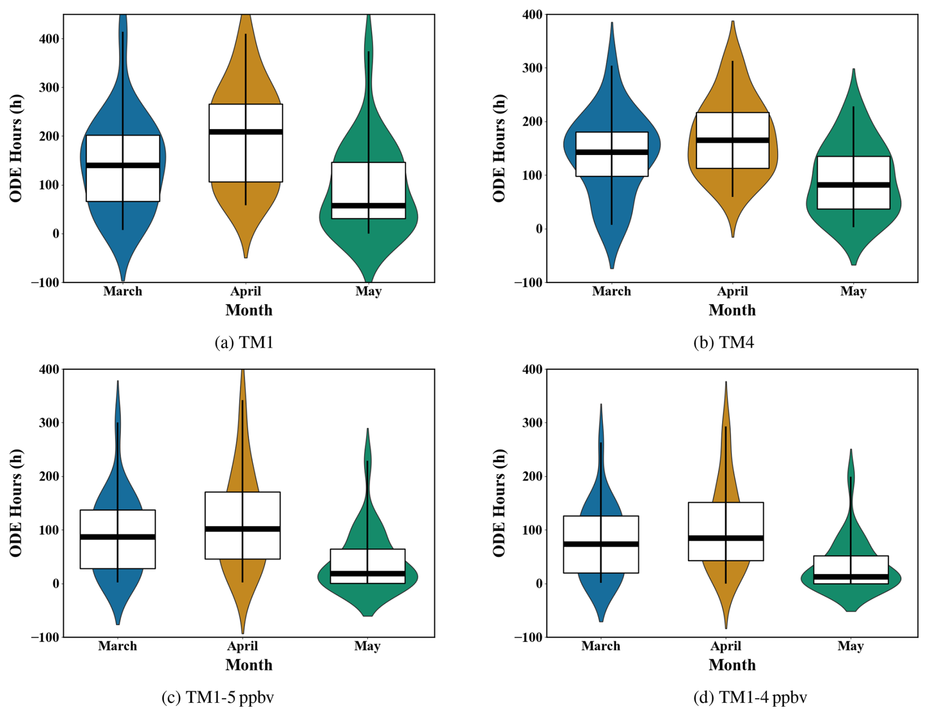
Figure 5 Monthly hours of ODEs for March, April, and May across the 23-year period from 2000 to 2022. The ODE hours were screened by (a) TM1, (b) TM4, (c) TM1–5 ppbv, and (d) TM1–4 ppbv.

When the TM4 criterion (ozone below $\mathrm{0.42}\stackrel{\mathrm{‾}}{\left[{\mathrm{O}}_{\mathrm{3}}\right]}$ for a start hour and a following hour within a 6 h period) was applied (Fig. 5b), we found that the order of the medians for these three months remained unchanged (April > March > May), compared with the results of TM1. However, we found that the ODE hours in April decreased while the hours in May increased when TM4 was applied. The data are also more concentrated. This is because TM4 uses a threshold that depends on the monthly averaged value. As the average ozone level in April is lower compared with those in March and May, using this relative criterion would exert a more stringent threshold than the constant 10 ppbv so that it screens out fewer ODE hours than TM1. For May with a high ozone level, the relative criterion is easier to achieve compared to the constant 10 ppbv criterion. Therefore, TM4 identifies more ODE hours in May compared to TM1. In summary, the TM4 method can screen out more ODE hours in months with high ozone values than TM1, and vice versa.

When 5 ppbv was used to replace the 10 ppbv threshold (i.e., TM1-5 ppbv, see Fig. 5c), we found that the order of ODE hours across the three spring months remained unchanged (April > March > May). However, the ODE hours for each month were significantly lower compared to those identified by TM1, due to the stricter threshold applied. Furthermore, the discrepancy in ODE hours between March and April was found to be less pronounced than that in the TM1 results, rendering the ODE hours in March (median: 87 h) and April (median: 102 h) very close. This indicates that the primary cause for the significantly greater number of ODE hours in April compared to March, as identified by TM1, was the more frequent occurrence of ozone concentrations falling within the 5–10 ppbv range in April than in March. With respect to the situation in May, the implementation of the 5 ppbv threshold resulted in a significant reduction to almost zero ODE hours. This finding suggests that ODEs characterized by very low ozone levels (<5 ppbv) have nearly vanished in May in recent years, which could be linked to global warming, resulting in higher temperatures during May, thereby causing the ODE season to cease earlier than before (Burd et al., 2017). Results obtained using the 4 ppbv threshold (Fig. 5d) are similar to those using the 5 ppbv threshold, except that the discrepancy in ODE hours between March (median: 73 h) and April (median: 85 h) is even less pronounced, thereby confirming the conclusions drawn above.

Figure 6 presents the yearly variability of the ODE hours for each spring month and the entire spring season, spanning from 2000 to 2022. It is seen from Fig. 6a that, based on the results of TM1, ODE hours in spring decreased significantly across these 23 years (p<0.05). This decreasing trend is mostly caused by the decline in ODE hours in April (see Fig. 6e), which is highly significant (p<0.01). In contrast to April, the drops in ODE hours in March and May were not significant (p>0.1, Fig. 6c) and close to significant ($\mathrm{0.05}<p<\mathrm{0.1}$, Fig. 6g), respectively. Our findings are in good agreement with those of Law et al. (2023), who reported a notable increase in observed surface ozone levels during spring from 1993 to 2019 at BRW, with the most significant increase observed in April. Hung et al. (2025) also observed an increasing trend in Arctic spring ozone concentrations at Eureka, Nunavut, Canada (80° N, 86° W) from 2008 to 2022, further supporting the notion of declining ODE frequency in the Arctic. Burd et al. (2017), in their study on the Arctic BrO season, found a decrease in BrO concentrations and an early end of the BrO season at BRW from 2012 to 2016, which may also imply a reduction in the occurrence of ODEs, aligning with our findings.

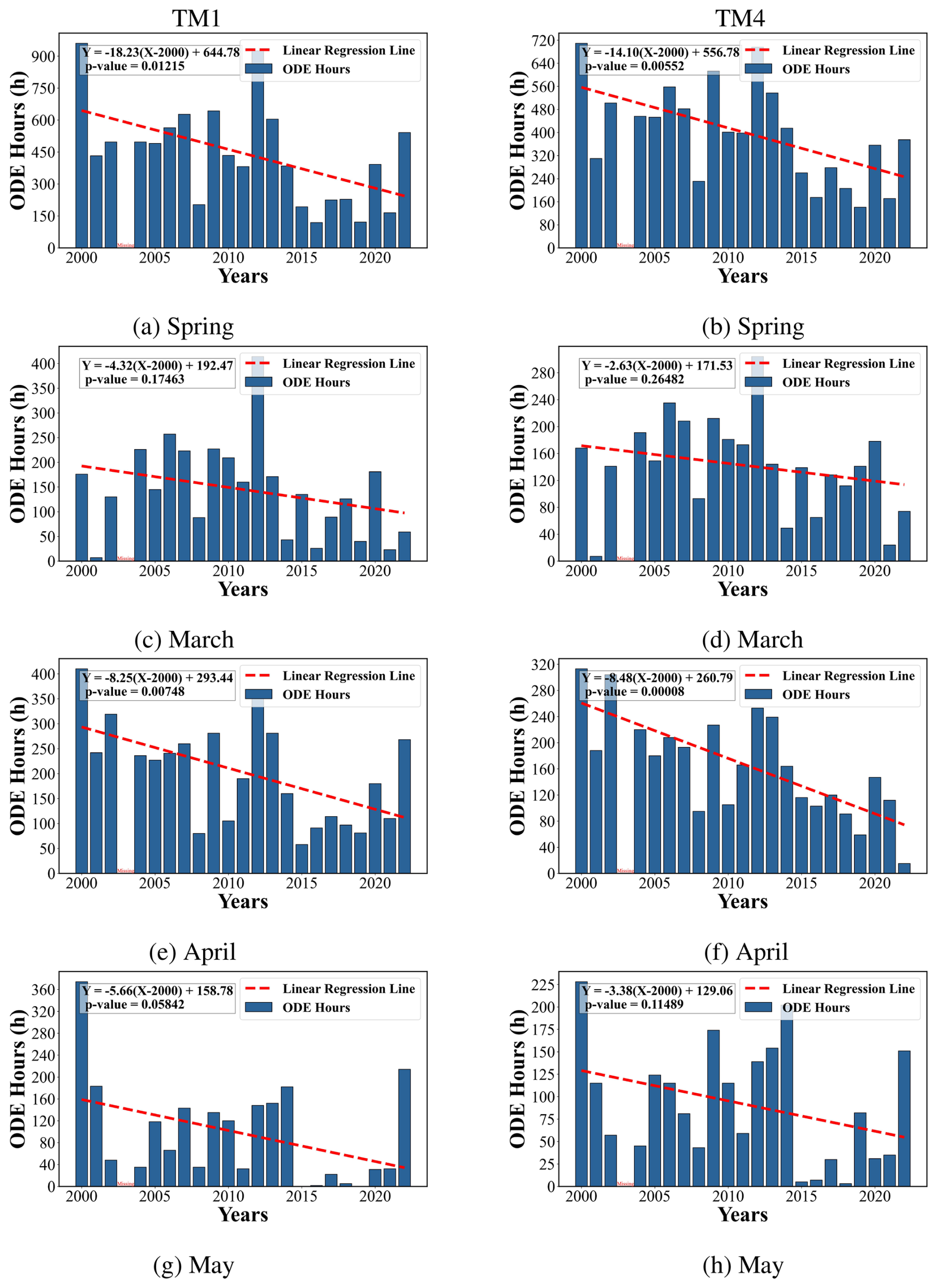
Figure 6 Yearly variability of ODE hours at the BRW Station, identified by two different criteria. Panels (a), (c), (e), and (g) show the ODE hours screened by the TM1 method for the whole spring, March, April, and May, respectively, while panels (b), (d), (f), and (h) show the hours screened by the TM4 method. Red dashed lines represent linear regressions of the ODE hours. The regression equations and p values are also provided.

The results of TM4 are similar (Fig. 6b) but show a more significant declining trend. The decrease in ODE hours in the entire spring season was highly significant (p<0.01) in the results of TM4, and the p value in April was also smaller, confirming the highly significant decline in ODE hours in April at BRW over the 23-year period. Aside from that, the drop in ODE hours in May was found to be insignificant (p>0.1) in TM4's results, whereas in TM1's results, the drop in May approached statistical significance ($\mathrm{0.05}<p<\mathrm{0.1}$).

When more rigorous thresholds (5 and 4 ppbv) were applied instead of the 10 ppbv threshold (refer to Fig. S6), the reduction in ODE hours in the entire spring season was found to be highly significant (p<0.01), denoting a more remarkable decline in the occurrence of severe ODEs with very low ozone levels during these years. This remarkable decline was still mainly attributable to the highly significant reduction in ODE hours in April (p<0.01). The decrease in March remained statistically insignificant, while the decline in May was identified as insignificant (p>0.1) for the 5 ppbv threshold and close to significant ($\mathrm{0.05}<p<\mathrm{0.1}$) for the 4 ppbv threshold, respectively.

In summary, results utilizing different criteria all indicate a decline in ODE hours during the spring season over the 23-year period, primarily driven by the highly significant reduction in April. However, when employing the threshold that varies with the monthly average ($\mathrm{0.42}\stackrel{\mathrm{‾}}{\left[{\mathrm{O}}_{\mathrm{3}}\right]}$) or more stringent fixed thresholds (5 ppbv and 4 ppbv), the results showed a more significant decline in ODE hours in spring, compared to those using the 10 ppbv threshold.

3.4 Relationship between ODE hours and meteorological parameters

We then investigated the relationship between ODE hours and surface meteorological parameters measured at the BRW Station. Figure 7 shows the wind information during the investigated spring seasons (Fig. 7a) and the time periods of ODEs identified by TM1 (Fig. 7b) and TM4 (Fig. 7c). From Fig. 7a, we can see that the prevailing wind at BRW is northeasterly in the springtime. The wind speeds were relatively higher when the winds were easterly (9–12 m s⁻¹ at most) and northeasterly (>12 m s⁻¹ at most). In contrast, wind speeds along other directions are mostly lower than 9 m s⁻¹. Compared to the wind speeds throughout the whole spring, Fig. 7b shows that during ODEs, the wind speeds are significantly lower (below 9, mostly 3–6 m s⁻¹), denoting a favored moderate wind speed condition for ODEs at BRW. Moreover, the wind direction tends to favor the northeasterly and northerly winds during ODEs, which are associated with the fresh sea ice covering the ocean to the north of BRW (Bottenheim and Chan, 2006; Gilman et al., 2010; Oltmans et al., 2012; Peterson et al., 2016). Additionally, we also found an increased proportion of westerly winds and a decreased proportion of easterly winds in Fig. 7b, denoting a favored westerly wind condition for ODEs at BRW. In an earlier study by Oltmans et al. (2012), they suggested that ODEs at BRW are predominantly associated with easterly winds, a finding that contrasts with the conclusions drawn in this study. The discrepancy between our findings and those of Oltmans et al. (2012) may originate from the different time periods investigated in these two studies. Moreover, a recent flight campaign originating from BRW (Brockway et al., 2024) also detected elevated levels of BrO being advected from the west of BRW, suggesting a potential transport of ozone-depleting air from the western direction. Additionally, in our recent modeling study on ODEs at BRW (Cao et al., 2023), we also found an ozone-depleting air mass transported to the BRW Station from the southwest under the influence of a cyclone moving eastward. The results obtained by applying the TM4 criterion (Fig. 7c) are also similar, confirming our findings.

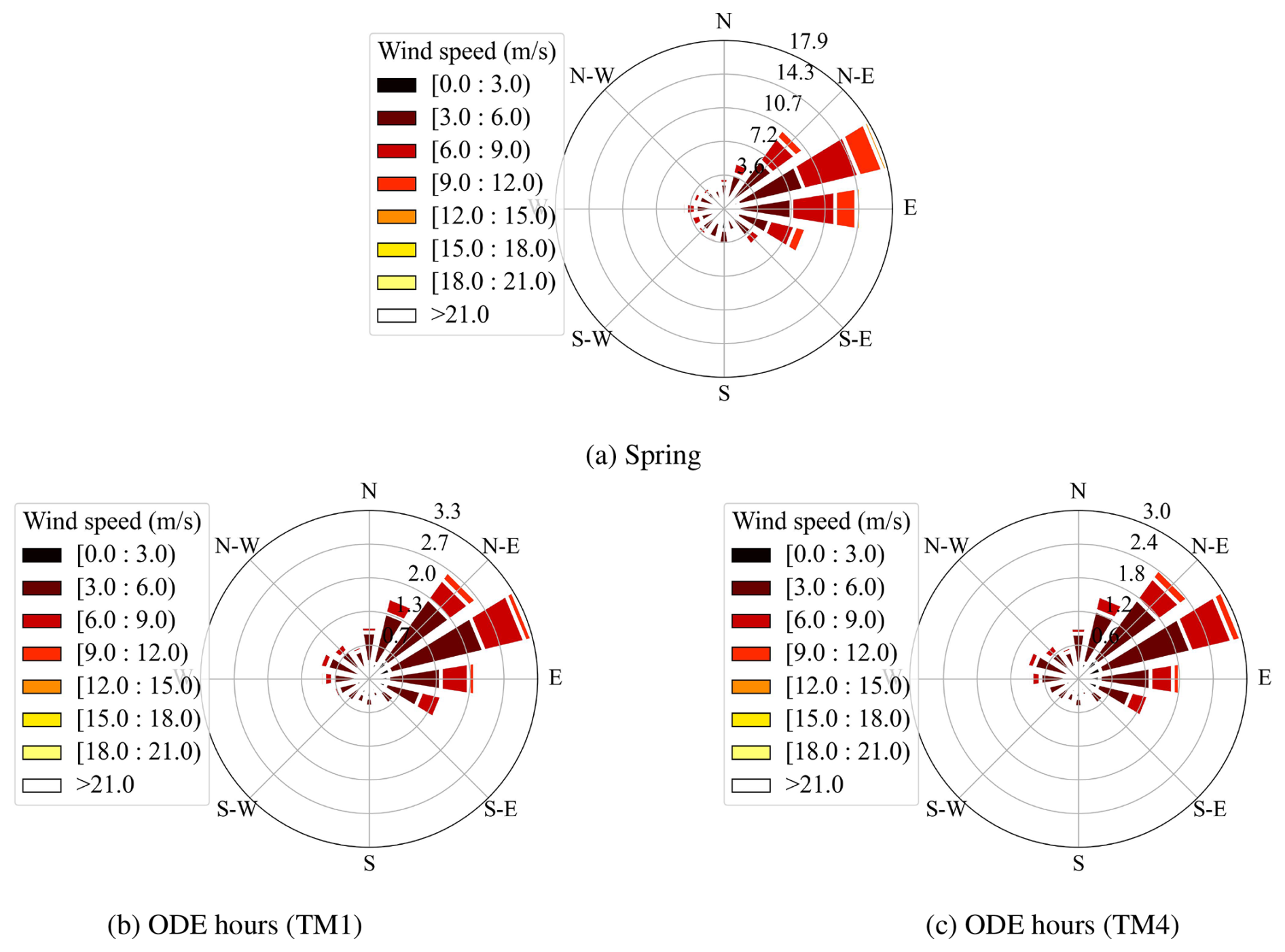
Figure 7 Wind rose diagrams during (a) the investigated spring seasons from 2000 to 2022 and ODE time periods identified by (b) TM1 and (c) TM4.

Results utilizing the 5 and 4 ppbv thresholds (refer to Fig. S7) also suggested that northerly and northeasterly wind conditions facilitate the occurrence of ODEs at BRW. However, the relative fractions of moderate wind speeds (3–6 m s⁻¹) and low wind speeds (0–3 m s⁻¹) during the identified ODE periods were higher than those found in the TM1's results, indicating that lower wind speeds are conducive to the occurrence of more severe ODEs, characterized by very low ozone levels.

The connections between ODE hours and the 2 m temperature measured at BRW are shown in Fig. 8, and the results obtained by applying TM1 (Fig. 8a) and TM4 (Fig. 8b) are similar. It was found that in the range of 250–272 K, the temperature at BRW generally exhibited a uniform distribution. However, occurrences of ODEs were more frequent at a lower temperature, with the highest occurrence frequency at approximately 250 K. Moreover, when the temperature was lower than approximately 256 K, the decrease in the 2 m temperature substantially enhanced the occurrence of ODEs (see the blue dot–dash lines in Fig. 8a and b). Thus, a lower temperature condition can facilitate the occurrence of ODEs, which is possibly associated with the stability of the boundary layer (Lehrer et al., 2004; Koo et al., 2012). It could also be linked to the effective absorption of HOBr on frozen $\mathrm{NaCl}/\mathrm{NaBr}$ surfaces at temperatures below the eutectic point of NaCl⋅2H₂O (i.e., 252 K), as reported by Adams et al. (2002). Below this temperature, a quasi-brine layer, characterized by its high acidity (Cho et al., 2002), is likely to develop on the ice/snow surface, which would promote bromine activation and subsequent ozone depletion. This lower temperature condition, favored by the bromine explosion and the ozone depletion, was also reported by Zilker et al. (2023), who applied a composite analysis on long-term ozonesonde data (2010–2021) and surface measurements over the Svalbard area in the Arctic.

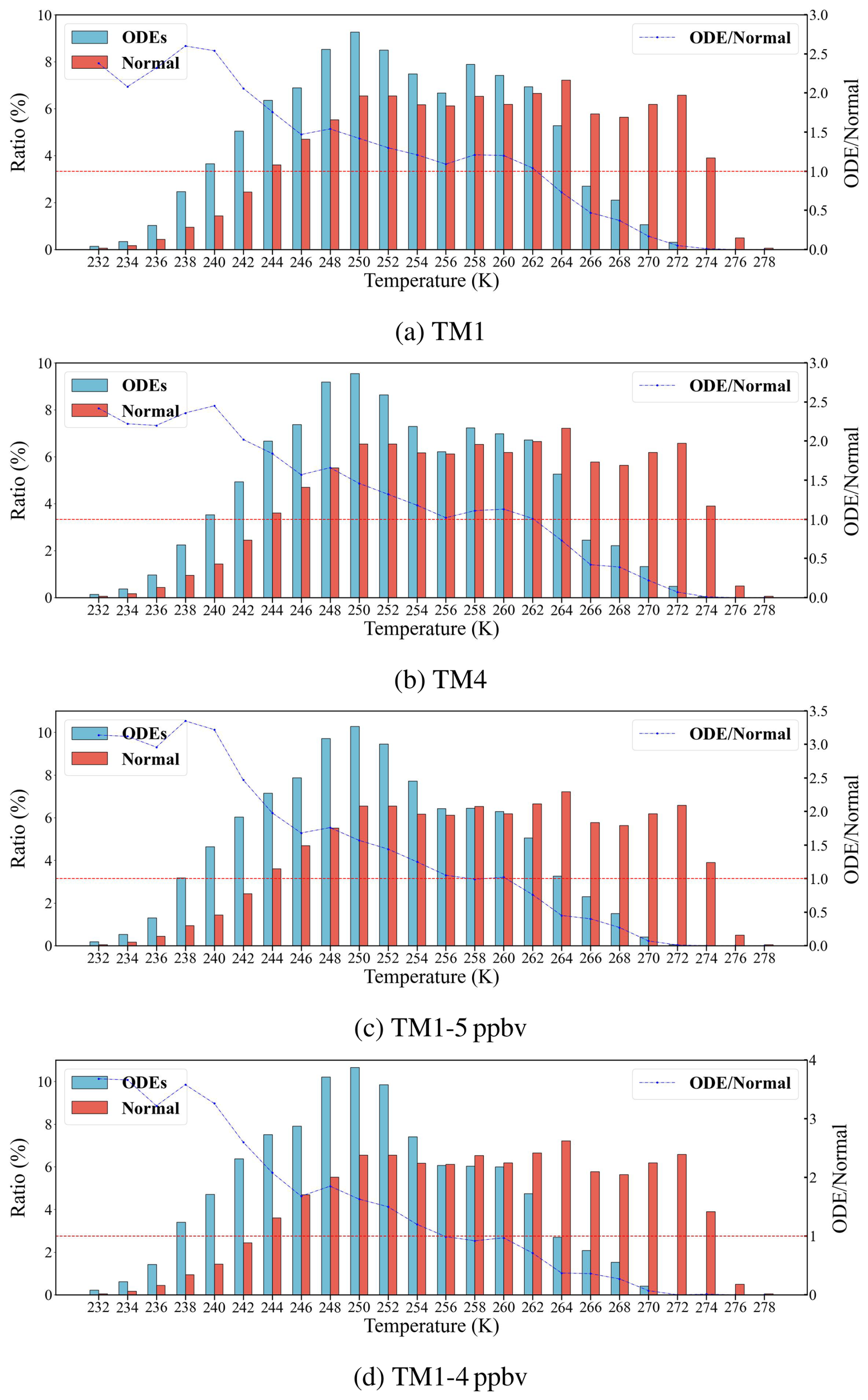
Figure 8 Occurrence frequency of ODEs versus the 2 m temperature. The ratio was calculated as the number of hours within each interval divided by the total number of hours. ODE hours used to calculate the ratio in panels (a), (b), (c), and (d) were screened by TM1, TM4, TM1–5 ppbv, and TM1–4 ppbv, respectively. The blue dot–dash lines denote the ratio of ODEs to normal conditions, and a value greater than 1.0 indicates a favorable condition for ODEs.

Results obtained by applying TM1–5 ppbv and TM1–4 ppbv (Fig. 8c and d) also indicate that ODEs are favored by low temperature conditions. More interestingly, Fig. 8c and d reveal a significant reduction in the occurrence frequency of severe ODEs within the temperature range of 256–262 K, when compared to TM1's results (Fig. 8a). This suggests that severe ODEs are more likely to occur only at temperatures below 256 K.

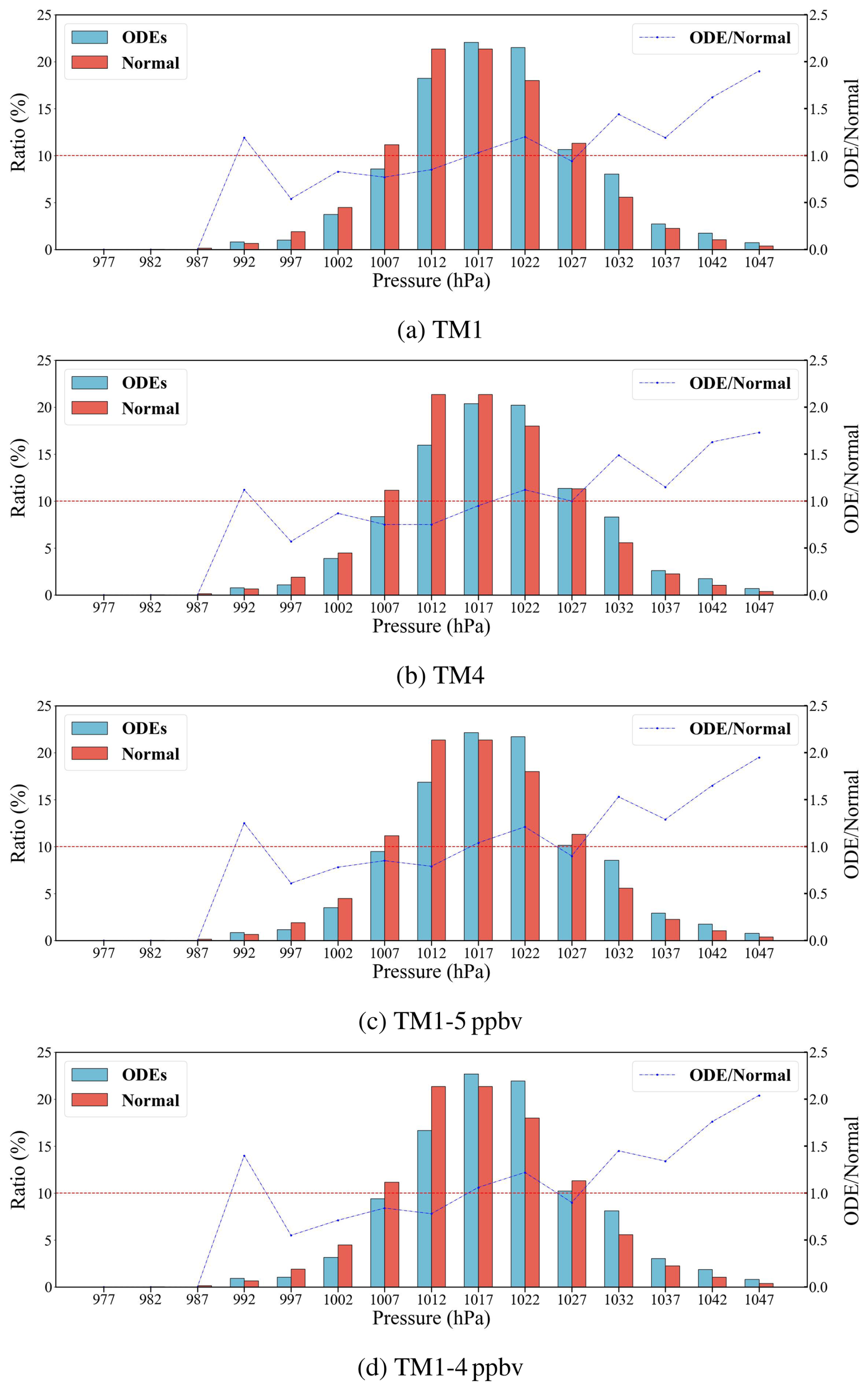
Figure 9 shows the relationship between the surface pressure at BRW and the occurrence of ODEs. Results obtained by using various criteria are largely consistent, exhibiting only slight differences. We found the occurrence of ODEs mostly within the pressure range of 1012–1027 hPa. Furthermore, an increase in surface pressure at BRW is often associated with a more frequent occurrence of ODEs, possibly due to the stable and calm conditions that prevail under the control of high-pressure systems. Additionally, it can be seen in Fig. 9 that when the surface pressure falls within the range of 990–995 hPa, the occurrence of ODEs is also favored (with the ratio ODE$/$Normal >1.0). It might be connected to the blowing snow events (Yang et al., 2010, 2019, 2020; Huang et al., 2018, 2020) when low-pressure systems (e.g., cyclones) pass by, which are beneficial for BrO release and the subsequent ozone depletion (Begoin et al., 2010; Zhao et al., 2016).

Figure 9 Occurrence frequency of ODEs versus surface pressure. The other settings for this figure are similar to those in Fig. 8.

4 Conclusions and future work

In this study, we investigated the influence of applying various criteria to identify springtime tropospheric ozone depletion events (ODEs) at Utqiaġvik (BRW), Arctic, using observational data from 2000 to 2022. We tested three types of criteria – traditional methods, variability-based methods, and machine learning methods – and analyzed the characteristics of these criteria in depth.

We found that the criteria using a constant threshold (e.g., 10 ppbv) and using thresholds based on the monthly averaged ozone values were more suitable for identifying ODEs at BRW than the other criteria. In contrast, the criterion considering both the mean value and standard deviation of ozone (i.e., the VM criterion) was able to identify time points when the surface ozone dropped to an uncommonly low level instead of a fixed threshold, which made it more adaptive and sensitive. However, extra caution is required when determining the parameter value of this criterion. Apart from these criteria, the machine learning method adopted in this study (i.e., the IF method) can automatically detect ODE hours, but this method has poor interpretability in screening results and sometimes was unable to correctly identify ODE hours when ODEs occur very frequently. Furthermore, the criteria proposed as suitable for identifying ODEs indicate an overall decreasing trend in the occurrence frequency of ODEs at BRW over this 23-year period, with the most significant decline observed in April. This suggests a potential impact of climate change, such as global warming and Arctic sea ice melting, on ODE occurrences. This declining trend of ODEs can lead to a weakening of the deposition of active mercury (Hg(II)), which is highly toxic and can pose serious health risks to humans. Therefore, the decline in ODE frequency could lead to a reduction in the health hazards associated with mercury deposition in mid-latitude regions. However, results obtained by implementing a threshold that varies with the monthly average, or by applying more stringent thresholds (5 and 4 ppbv), showed a more significant reduction in the occurrence of ODEs compared to those using the 10 ppbv threshold. Thus, using a different criterion to identify ODE hours may lead to different conclusions. This is why we tested various ODE criteria, compared the resulting conclusions, and attempted to propose suitable criteria for identifying ODEs in this study.

Applying suitable criteria also enables us to study the connection between meteorological conditions at BRW and the occurrence of ODEs more precisely. ODEs at BRW were found to be more likely to occur under northerly and northeasterly winds, with moderate wind speeds (mostly 3–6 m s⁻¹) being more favorable, although ODEs were also observed at higher wind speeds (6–12 m s⁻¹). Lower wind speed conditions were also found to facilitate the occurrence of more severe ODEs, characterized by very low ozone concentrations. ODEs were also found to be closely linked to temperature and pressure. ODEs, especially the severe ones, tend to occur at temperatures lower than 256 K, which may be associated with the stability of the boundary layer and the effective absorption of HOBr on frozen surfaces, promoting bromine activation and subsequent ozone depletion. Additionally, ODEs at BRW tend to occur under high-pressure conditions (>1010 hPa), indicating that the high-pressure-associated weather conditions may facilitate the occurrence of ODEs.

In the future, we would like to improve the machine learning methods (e.g., Isolation Forest) so that a more reliable method can be applied in ODE identification. Moreover, the present analysis can also be extended to a longer time series of data to provide a more comprehensive understanding of the long-term trends and variability of ODEs in the Arctic. Conclusions obtained in this study should also be verified at other Arctic stations. To achieve this goal, we gathered more observational data from seven other Arctic sites (Alert, Esrange, Tustervatn, Villum, Pallas, Summit, and Zeppelin) aside from the one (BRW) we initially focused on in this study. After applying the criteria using constant values (10 and 5 ppbv) that were proposed in this study, only four of these sites (Alert, BRW, Villum, and Zeppelin) were found to have ODE occurrences (see Fig. S8 in the Supplement). We found that the ODE hours screened out by the criteria proposed in this study were appropriate. For instance, BRW, which has a low altitude, is characterized by a high frequency of ODE occurrence. In contrast, Zeppelin, which is located at a higher altitude, has fewer ODE hours, because the air mass arriving at Zeppelin usually represents the air in the free troposphere, so that more ozone can be transported from the stratosphere and fewer halogens released from the surface can reach the free troposphere due to the barrier at the top of the boundary layer. Additionally, the ODE curves for Villum also show a declining trend, which is consistent with the conclusion drawn in this study. However, more observational data for other species, such as halogen species (i.e., BrO) from satellite detection and ground-based multi-axis differential optical absorption spectroscopy (MAX-DOAS), are still needed to validate these results and help identify ODEs more accurately. Unfortunately, we currently do not have access to such data, which is also a limitation of the present study.