Microphysical parameter choices modulate ice content and relative humidity in the outflow of a warm conveyor belt

Warm conveyor belts (WCBs) play a crucial role in Earth's climate by transporting water vapor and hydrometeors into the upper troposphere/lower stratosphere (UTLS), where they influence radiative forcing. However, a major source of uncertainty in numerical weather prediction (NWP) models and climate projections stems from the parameterization of microphysical processes and their impact on cloud radiative properties as well as the vertical re-distribution of water. In this study, we use Lagrangian data from a perturbed parameter ensemble (PPE) of a WCB case study to investigate how variations in microphysical parameterizations influence water transport into the UTLS and the outflow cirrus properties. We find that the thermodynamic conditions (pressure, temperature, specific humidity) at the end of the WCB ascent show little sensitivity to the explored parameter perturbations. In contrast, ice content and relative humidity exhibit substantial variability, primarily driven by the capacitance of ice (CAP) and the scaling of ice formation processes directly influenced by ice-nucleating particle (INP) concentrations. Different combinations of CAP and INP scaling yield vastly different ice and relative humidity distributions at the end of the ascent and in the subsequent hours. These differences are particularly pronounced in fast-ascending air parcels, where modifications to the saturation adjustment scheme (SAT) introduce small variations in pressure and temperature at the end of ascent. Our findings have potential implications for parameter choices in cloud models and considerations for geoengineering strategies. Future comparisons with high-quality observational data could help constrain the most realistic parameter choices, ultimately improving weather and climate forecasts.

1 Introduction

The most dominant greenhouse gas is water vapor (Schneider et al., 2010), and in the upper troposphere/lower stratosphere (UTLS) region, changes in its concentration lead to the most important positive feedback mechanism for climate change (e.g. Li et al., 2024; Held and Soden, 2000; Dessler et al., 2013). Even small changes in UTLS water vapor content can significantly alter the Earth's radiative budget (Wang et al., 2001; Hansen et al., 1984) and impact the mean and regional circulation patterns (e.g. Charlesworth et al., 2023; Ploeger et al., 2024). It is therefore crucial to quantify (i) the amount and regional distribution of moisture in the UTLS (and how this has changed over time), (ii) the contributions of different transport pathways delivering moisture to the UTLS, and (iii) how these factors are likely to change in the future.

Although UTLS water vapor measurements have increased over the past 20 years (Zahn et al., 2014; Jeffery et al., 2022; Hurst et al., 2011; Tilmes et al., 2010; Konjari et al., 2024), the UTLS remains poorly characterized due to challenging measurement conditions (Jeffery et al., 2022) as well as instrument uncertainties, with calibrated measurements typically only accurate to within 5 %–10 % in supersaturated regimes (Petzold et al., 2020). In situ measurements from aircraft and balloon-borne instruments provide high vertical resolution data on water vapor, but their limited regional and temporal coverage makes performing extensive climatologies difficult (Kunz et al., 2008; Zahn et al., 2014; Jeffery et al., 2022; Hurst et al., 2011). Satellite instruments offer long-term, global datasets, but they face challenges such as coarse vertical resolution and path length limitations (Hegglin et al., 2008, 2021). Therefore, accurate measurement and quantification of UTLS moisture, as well as changes over time, and quantification of its role in climate, remains a pressing and difficult challenge.

Moisture is transported to the UTLS through several pathways, with deep convection in the tropics being a major contributor. Both experimental (Corti et al., 2008; Danielsen, 1993; Lee et al., 2019; Gordon et al., 2024) and modeling studies (Ueyama et al., 2018, 2023; Dauhut et al., 2018; Hassim and Lane, 2010) have shown that UTLS moistening by convection occurs not only through the direct transport of water vapor but also via the sublimation of ice crystals detrained from convective clouds. Climate models predict that UTLS humidity will increase as the climate warms due to the warming of the tropopause (Gettelman et al., 2010), but Dessler et al. (2016) also determined that a large part of this can be attributed to the increase in sublimation of convective ice. It remains unclear how convective transport of moisture to the UTLS will change in the future, but a historical climatology by Jeske and Tost (2025) found that the height of convective outflow has shifted to lower pressures from 2011 to 2020 compared to the 1980s. While most of the aforementioned studies provide valuable insights into UTLS moisture transport and changes thereof, they focus primarily on the tropics.

Although more sparse, smaller in scope, and subject to large uncertainties, there have been studies investigating the transport of moisture in the extratropics. Homeyer et al. (2024) examined extratropical stratospheric hydration processes using observations over the continental United States, while Homeyer et al. (2014) and Homeyer (2015) conducted model analyses of overshooting convection in the same region. Heller et al. (2017) examined measurements from a case study of mountain waves over the Southern Alps in New Zealand and found evidence of vertical water vapor flux, suggesting that mountain waves have the potential to affect the water vapor distribution in the UTLS. Using satellite data, Sun et al. (2017) characterized seasonal and decadal changes in UTLS water vapor over the Tibetan Plateau, and found that in the summer, water vapor increased due to convective transport as determined by Fu et al. (2006). Globally, and covering the years from 2002 to 2012, Weigel et al. (2015) validated the SCIAMACHY satellite dataset to other satellite and in-situ measurement and found them to be reliable for altitudes between 15 and 23 km. However, and crucially, in the extratropics and for altitudes between 11 and 15 km, the mean percentage differences to other datasets exceeds 50 %. To determine the main transport pathways for UTLS water vapor, Zahn et al. (2014) conducted a multi-year analysis of monthly UTLS water vapor measurements and identified warm conveyor belts (WCBs) as a key contributor to extratropical UTLS moisture. A recent climatological study by Guo and Miltenberger (2025) managed to quantify this contribution, and they determined that in December, January and February the moisture transported in WCBs by grid-scale advection accounts for up to 13.8 % (23.3 %) of the total water (condensate) transport into the upper troposphere above the North Atlantic and Pacific ocean basins.

Warm conveyor belts (WCBs) are large-scale, coherently ascending airstreams that develop near extratropical cyclones (ETCs) and generate the characteristic elongated cloud bands associated with ETCs (Madonna et al., 2014). Over approximately two days WCBs transport moist air from the boundary layer poleward and upward into the upper troposphere, while the air mass undergoes complex microphysical and dynamical processes. These processes contribute to precipitation formation, influence upper-level wave propagation, and inject water vapor and hydrometeors into the UTLS. As a result, WCBs play a crucial role by shaping mid-latitude weather systems, modulating storm development, and affecting Earth's radiative budget through cloud formation and moisture transport (Madonna et al., 2014). The ascending air produces significant amounts of precipitation, which can be hazardous (Pfahl et al., 2014); notably, WCBs account for more than 80 % of the total precipitation in Northern Hemispheric storm tracks (Pfahl et al., 2014; Eckhardt et al., 2004; Binder et al., 2016). In addition to producing precipitation, WCBs transport considerable amounts of energy as well as water vapor, hydrometeors, aerosols and trace gases across latitudes, and influence large-scale weather patterns (Joos et al., 2023; Madonna et al., 2014; Rodwell et al., 2018). The diabatic heating experienced by the ascending air masses affects cyclone strength and lifetime (Binder et al., 2016; Rossa et al., 2000; Binder et al., 2023) and produces potential vorticity (PV) anomalies (Oertel et al., 2020; Methven, 2014) that could influence atmospheric blocking (Pfahl et al., 2015; Wandel et al., 2024) and Rossby wave evolution (Pickl et al., 2023; Grams et al., 2011; Joos and Wernli, 2011; Wernli, 1997). Given that WCBs exert such wide-ranging influences, forecast skill is highly sensitive to how well models capture their path, vertical extent, diabatic-heating profile and mixed-phase cloud evolution, and any uncertainty in representing these aspects can quickly degrade predictions of cyclone intensity, heavy-precipitation placement, downstream wave development, and even heat waves (Pickl et al., 2023; Berman and Torn, 2019; Rodwell et al., 2018; Grams et al., 2018; Oertel et al., 2023).

WCBs influence Earth's radiative budget in multiple ways. During the early stages of ascent, when WCBs are usually located closer to the equator than during later stages, low-level clouds predominantly exert a cooling effect. As the WCB progresses northward, high-level frozen clouds have a warming or cooling effect depending on solar insolation, cirrus optical thickness, and potentially cloud overlap (Krämer et al., 2020; Joos, 2019; Johansson et al., 2019). In between, mixed-phase clouds have an uncertain net radiative effect. The outflow region of a WCB is also often accompanied by ice-supersaturated regions (Spichtinger et al., 2005) and an up to 3 km deep cirrus cloud shield (Binder et al., 2020), that has an net warming effect on average. Consequently, determining which overall effect dominates and how this balance may shift in the future remains a challenge (Joos, 2019). Additionally, it remains unclear how the transport of water vapor into the UTLS by WCBs will change in the future. For these reasons, accurately representing WCBs in NWP models is crucial for both weather and climate predictions.

However, accurately representing WCBs is challenging, partly because the ascending air undergoes a wide range of warm-phase, mixed-phase, and cold-phase microphysical processes (Binder et al., 2020; Forbes and Clark, 2003; Gehring et al., 2020), producing clouds with varying phases that add significant complexity to the model representation (Oertel et al., 2023; Schwenk and Miltenberger, 2024; Hieronymus et al., 2025). Additionally, the ascent occurs across different time-scales, which result in different dominating microphysical processes (Schwenk and Miltenberger, 2024). The precise composition of WCB clouds at different stages of the ascent is therefore difficult to determine and to represent in NWP models, and hence the parameterizations of the microphysical processes within them are a major source of uncertainty (Morrison et al., 2020; van Lier-Walqui et al., 2012; Posselt and Vukicevic, 2010; Oertel et al., 2025). Sensitivity experiments have demonstrated that the choice of microphysical parameterization schemes can significantly affect the characteristics of WCB ascent (Mazoyer et al., 2021, 2023), and that the diabatic processes occurring during WCB ascent are also sensitive to the specific choice of cloud microphysical parameters in a given parameterization scheme (Hieronymus et al., 2022; Neuhauser et al., 2023; Forbes and Clark, 2003). Classical sensitivity experiments, such as Monte Carlo simulations, could theoretically assess how specific parameterized processes contribute to uncertainties. However, applying these methods to NWP models across a large free parameter space, as typical for e.g. cloud microphysical parameterisations, is impractical due to their high computational cost and the vast amounts of data they produce. This has led to the employment of Perturbed Parameter Ensembles in atmospheric sciences (PPEs e.g., Lee et al., 2011; Collins et al., 2010; Johnson et al., 2015; Oertel et al., 2025), which are sensitivity experiments that sample the multi-parameter phase space spanned by the uncertain parameter values in a statistically optimal manner with a relatively small number of simulations.

In this paper we make use of a novel and unique PPE for a WCB case produced by Oertel et al. (2025), in which four cloud microphysical parameters and one parameter related to WCB inflow properties were modified. Oertel et al. (2025) specifically investigated (i) how the uncertainties in microphysical parameters influence the representation of WCB ascent and (ii) how the perturbed parameters affect the precipitation structure and larger-scale flow evolution. Our goal is to determine how microphysical parameter choices affect the transport of moisture and hydrometeors by ascending WCB air parcels into the UTLS. Schwenk and Miltenberger (2024) found that in the outflow of a WCB, the specific humidity (q_v) of Lagrangian WCB air parcels is predominantly constrained by the thermodynamic conditions at the end of ascent (i.e, the temperature and pressure in alignment with the Clausius-Clapeyron relationship). Remarkably, these results suggest that WCB air parcels are very efficient at converting water vapor into hydrometeors, otherwise, greater or more widespread supersaturation would be produced. This observation raises the question if this efficiency in vapor conversion reflects a physical reality, or if it is an artifact of the NWP model's potentially inadequate representation of vapor conversion in ascending air parcels?

One potentially inadequate representation could be the ICON model's saturation adjustment scheme, which forces 100 % saturation over water at every model time step as long as the parcel contains any liquid water (by either evaporating cloud condensate or condensing excess vapor). However, in reality supersaturation over water can form under conditions of high vertical velocity. Making the saturation adjustment scheme more realistic by allowing for some supersaturation over water when vertical velocities are high might change the vapor conditions in the outflow of a WCB. However, most WCB air parcels glaciate completely during their ascent, meaning that they spend a lot of time in a purely ice phase (Schwenk and Miltenberger, 2024). In this case other parameters – such as the capacitance of ice (CAP) or CCN as well as INP concentrations – likely play a more significant role in determining the efficiency of vapor conversion. For instance, an increase in the capacitance could accelerate ice particle growth, while higher concentrations of CCN can lead to more and smaller cloud droplets in the liquid phase, which can in turn increase the number of ice crystals in the frozen phase and enhance vapor conversion. Similarly, a greater concentration of INP might result in a faster transition to the ice phase, further affecting the overall conversion process. If the perturbations can significantly influence the ice content, ice number concentration or cirrus lifetime in the WCB outflow, they could also alter the radiative budget of the WCB, which would be important to consider when analyzing the future impact of WCBs on global warming. Such impacts would also be relevant for potential geoengineering strategies, such as marine cloud brightening (Latham et al., 2012) or cirrus cloud thinning (Lohmann and Gasparini, 2017; Villanueva et al., 2022; Gasparini et al., 2020), which aim to modify CCN or INP levels to change the radiative properties of clouds. The findings obtained from this paper might provide valuable insights for future geoengineering efforts seeking to manipulate cloud properties to achieve climate-modulating effects.

An additional consideration for moisture transport in WCBs is the role of convectively ascending air parcels. Schwenk and Miltenberger (2024) compared the transport of water for fast (convective) and slow ascending WCB air parcels and found that rapidly ascending WCB air parcels carry substantial amounts of ice into the UTLS. This could have notable implications for the radiative budget of WCBs, since high level clouds can contribute to global warming (Haslehner et al., 2024), and–as discussed above–sublimating ice could increase the UTLS vapor content (Dessler et al., 2016). This raises two additional questions: (i) how do different parameter choices affect the mass and number of ice particles (or snow) transported into the UTLS differently for fast and for slow ascending air parcels, and (ii) how does moisture transport change when we change the fraction of convectively ascending air parcels (by modulating the SST)?

In summary, this article addresses the following research questions by analyzing a PPE of a WCB case: (How) do perturbations in microphysical parameters and SST (i) influence moisture conditions in the WCB outflow, (ii) alter hydrometeor distributions, particularly for ice, in the WCB outflow, and (iii) how do these effects vary with ascent velocity and (iv) evolve in the hours following the end of ascent?

2 Methods

The WCB trajectory data we investigate in this study are taken from a perturbed parameter ensemble (PPE) which is described in detail in Oertel et al. (2025). In this section, we provide a brief description of the ICON model setup, the design of the PPE, and an overview of the chosen parameter perturbations (Sect. 2.1, 2.2), as described by Oertel et al. (2025). We then proceed to explain how we select WCB trajectories and define the beginning and end of ascent (Sect. 2.3). Finally, we explain the statistical methods used to analyze the impact of parameter choices on model output (Sect. 2.4).

2.1 ICON model Setup and Lagrangian data

A global simulation with the Icosahedral Nonhydrostatic (ICON) modelling framework (Zängl et al., 2014; version 2.6.2.2) with approximately 13 km grid spacing (R03B07 grid) was run for 72 h, initialized from the ECMWF analysis at 18:00 UTC on 3 October 2016, with a 120 s time step. Two nested domains with grid spacings of approximately 6.5 km (R03B08) and approximately 3.3 km (R03B09) and time steps of 60 and 30 s, respectively, cover the WCB ascent region and interact with the global simulation via two-way feedback. All domains have 90 vertical model levels, and in the WCB outflow region (∼ 7–12 km) the vertical grid-spacing is between 200 and 400 m. The two moment cloud microphysics scheme from Seifert and Beheng (2006) is used, which contains six prognostic hydrometeor types (cloud liquid (q_c), rain (q_r), ice (q_i), snow (q_s), graupel (q_g) and hail (q_h)). In the global domain convection is parameterised with the Tiedke-Bechtold convection scheme (Tiedtke, 1989); in the higher-resolution nests only shallow convection is parameterised. For all other parameterisations the standard schemes are used (see Oertel et al., 2025). The described set-up is used to perform 70 simulations with varying lower boundary conditions and cloud microphysics parameters as detailed in Sect. 2.2.

The online trajectory module by Miltenberger et al. (2020) and Oertel et al. (2023) is used to calculate air-mass trajectories (see Schwenk and Miltenberger, 2024; Oertel et al., 2025 for details). Trajectories are started from six vertical levels between 200 and 1500 m every 1 h during the simulation in a longitude and latitude region (55 to −15° E, 35 to 55° N) predefined by prior offline trajectory calculations with LAGRANTO (Sprenger and Wernli, 2015). Trajectory data is stored every 1 h. This study exclusively analyzes the Lagrangian data obtained from the PPE.

A detailed overview of the synoptic situation and trajectory data is given in Oertel et al. (2023) and Oertel et al. (2025). Here, we provide a short summary. The extratropical cyclone that produced the WCB cloud band examined in this paper originated at approximately 40° W and 50° N in the early hours of 4 October 2016. It propagated in the Eastern direction and by 4 October 2016 12:00 UTC, a clear front formed at approximately 30° W (Fig. 1a). After this time, the typical comma-shaped WCB cloud band formed and the cyclone propagated to the Northeast, reaching Iceland and the southeastern Greenland shore at 5 October 2016 00:00 UTC (Fig. 1b). The WCB progressed further Northeast (Fig. 1c) and at 6 October 2016 00:00 UTC (Fig. 1d) it began to dissipate over the arctic.

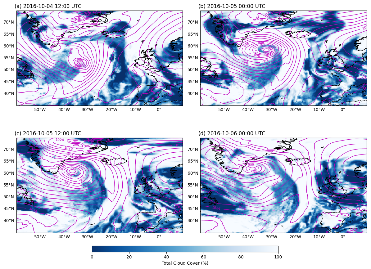
Figure 1 ERA5 data showing the total cloud cover and sea level pressure at 4 October 2016 12:00 UTC in (a), 5 October 2016 00:00 UTC in (b), 5 October 2016 12:00 UTC in (c) and 6 October 2016 00:00 UTC in (d).

2.2 Perturbed parameter ensemble design

The PPE designed by Oertel et al. (2025) simultaneously perturbs the values of five parameters, which are kept constant throughout the simulation. These parameters are sea surface temperature (SST), the capacitance of ice and snow (CAP), the impact of ice nucleating particle (INP) number concentration on ice formation, cloud condensation nuclei (CCN) number concentration, and the saturation adjustment scheme (SAT). The specific parameter combinations for individual PPE members are chosen such that the PPE optimally explores the entire phase space spanned by the selected parameters using a Latin hypercube design. In total, 70 PPE members are available. For an overview of each parameter see Oertel et al. (2025); here we only provide a brief overview and present the chosen parameter ranges in Table 1.

Table 1 Overview of parameter perturbations (taken from Oertel et al., 2025).

CAP: The capacitance of frozen hydrometeors (CAP) influences the rate at which water vapor deposits onto ice surfaces, thereby influencing the growth of ice and snow, the phase state of the water substance in an air parcel, and the associated latent heat release. While theory predicts a normalized CAP value of 0.5 for perfectly spherical particles, realistic ice and snow hydrometeors often exhibit considerably different values (Westbrook et al., 2008; Chiruta and Wang, 2003). Consequently, in the PPE, CAP for ice and snow is varied (simultaneously) by a scaling factoring ranging from 0.2 to 1, which explores a range for CAP from 0.1 to 0.5. CAP values for graupel and hail, which are assumed to be sufficiently spherical, are not changed.

INP: INP concentrations are important for cloud and precipitation formation, can alter cloud radiative forcing (CRF) (Schrod et al., 2020; Burrows et al., 2022), and their concentrations in the atmosphere vary over several orders of magnitude (Hande et al., 2015; DeMott et al., 2010). However, there are still large gaps in knowledge about their spatial, vertical and seasonal distributions and their representation in NWP models is highly uncertain (Wex et al., 2019, 2024; Schrod et al., 2020; Li et al., 2022). In the PPE, Oertel et al. (2025) did not directly perturb the INP concentrations that are calculated by the ICON model, but instead scaled three processes which are known to be directly influenced by INP number concentrations-immersion freezing of cloud droplets, deposition nucleation of ice, and freezing of rain drops-by applying a logarithmically spaced factor ranging from 0.01 to 20 to emulate varying INP concentrations. This scaling is designed to emulate scaling the number of INPs. In ICON, the heterogeneous freezing parameterization includes immersion freezing of cloud droplets (Hande et al., 2015), deposition nucleation of ice (Hande et al., 2015) and freezing of rain drops (Bigg, 1953). In this scheme, immersion freezing is active below −12 °C as long as cloud droplets are present. The number of activated INPs is a function of temperature, and the increase in ice-number concentration per time-step depends on the current and previous number of activated INPs. Deposition nucleation takes place in a temperature range from −20 to −53 °C and the number of activated INPs additionally depends on supersaturation with respect to ice (Lüttmer et al., 2025). For example: at −15 °C and 110 % relative humidity over ice, the immersion freezing INP concentration amounts to ≈5 m⁻³ for the unperturbed reference and varies between 1 and ∼100 m⁻³. The rate of freezing of rain is temperature dependent; below −40 °C all rain drops instantly freeze. Ice-formation parameterizations in ICON that remain unchanged in the PPE are (i) the homogeneous nucleation, parameterized following Kärcher and Lohmann (2002) and Kärcher et al. (2006), where the freezing rate and critical supersaturation are functions of temperature; (ii) homogeneous freezing of cloud droplets (Jeffery and Austin, 1997), where below −50 °C, all cloud droplets freeze instantly; and (iii) secondary ice production (Hallet and Mossop rime splintering), active between approximately −8 and −3 °C (Hallet and Mossop, 1974; Seifert and Beheng, 2006).

CCN: The cloud droplet activation scheme implemented in ICON was originally designed for continental Germany by Hande et al. (2016) and assumes a vertical CCN profile that decreases as pressure decreases. This profile does not change over time nor across the globe, and droplet activation scales with the resolved vertical velocity. However, it is known that CCN number concentrations are not constant, but vary in space and time, depending on factors such as the season and air mass origin (Schmale et al., 2018; Rose et al., 2021). Over continents they can also differ substantially from concentrations over the open ocean. Therefore, Oertel et al. (2025) used a modified cloud droplet activation scheme designed by Oertel et al. (2023) to account for CCN concentrations over the northern Atlantic. The details are described in the latter publication, but we point out that, in the new scheme, cloud droplet activation continues to scale with pressure and vertical velocity, and the profile remains the same globally (i.e. it is a tailored adjustment for an open-ocean WCB). In the unperturbed reference, the CCN concentration is approximately ∼250 cm⁻³ near the cloud-base (at ∼ 800 hPa) for large vertical velocities (see Fig. 2 in Oertel et al., 2023). In this PPE, the uncertainty in representing CCN number concentrations is accounted for by scaling the number of activated cloud droplets throughout the vertical profile at each model time step by a factor ranging from 0.4 to 20. This variation results in CCN concentrations varying from approximately 100 to 5000 cm⁻³, which approximately represents the variability that has been observed for CCN concentrations (Hande et al., 2015, 2016; Genz et al., 2020; Wang et al., 2021).

SAT: As discussed in the introduction, when a cloud contains liquid water, the saturation adjustment scheme used in ICON instantaneously removes supersaturation or in-cloud sub-saturation by condensing or evaporating excess or deficient water vapor until a relative humidity of 100 % over water is achieved. This becomes increasingly unrealistic when vertical velocities are high or CCN numbers very low (Lebo et al., 2012). In the PPE, the scheme is therefore modified to allow supersaturation over water to develop under conditions of strong vertical velocity. This modification is done by including a scaling factor f_SATAD, ranging from 0 to 0.1, which is multiplied with the vertical velocity (only when vertical velocities are larger than zero), added to one, and finally multiplied with the specific humidity from the default scheme:

$$\begin{array}{}\text{(1)}& q_{\mathrm{v},\mathrm{s}}^{*}(T,p)=\left(\mathrm{1}+\left(f_{\mathrm{SATAD}}\cdot w\right)\right)\cdot q_{\mathrm{v},\mathrm{s}}(T,p)\mid w>\mathrm{0}.\end{array}$$

A factor f_SATAD of 0 corresponds to the standard scheme, which inhibits the formation of supersaturated conditions. For a factor f_SATAD of 0.1, vertical velocities of 2 m s⁻¹ can produce supersaturations of 20 %, which aligns with theoretical examinations of supersaturation in liquid clouds (Korolev and Mazin, 2003; Morrison and Grabowski, 2008).

SST: Tropospheric humidity in the inflow region of a WCB is crucial for the subsequent ascent (Schäfler and Harnisch, 2014; Christ et al., 2025; Berman and Torn, 2022, 2019) and formation of precipitation (Dacre et al., 2019). Yet NWP models can have substantial humidity errors (Schäfler et al., 2010, 2011). Since the moisture content of marine boundary-layer air is mostly controlled by temperature, the PPE modifies SST (which in ICON is kept constant throughout the simulation) within the range of ±2 K to analyze the sensitivity to both the temperature and moisture in the WCB inflow region. A difference in SST can also be seen as analogous to a shift in latitude or as an uncertainty in cyclone position or WCB inflow location.

2.3 Trajectory selection and ascent time characterisation

WCB trajectories must fulfill the criteria of ascending at least 600 hPa within 48 h. We use the widely used ascent time-scale τ₆₀₀, defined as the shortest time taken per trajectory to ascend at least 600 hPa, to characterise the ascent time of a WCB trajectory. As we are most interested in the characteristics of trajectories once they have completed their ascent and have entered the UTLS, we do not only consider the τ₆₀₀ ascent-segment, but the entire time around this segment during which the ascent velocity remains above 8 hPa h⁻¹ (using the algorithm described by Schwenk and Miltenberger, 2024). We refer to this time as τ_WCB. The end of ascent is defined as the last time-step in τ_WCB. Note that in contrast, Oertel et al. (2025) consider the τ₆₀₀ segment.

2.4 Methods for quantifying parameter perturbation impacts

The impact of parameter perturbations are investigated for selected properties of WCB outflow (target variables): temperature, pressure, specific humidity, relative humidity over ice and hydrometeor content at (i) the end of WCB ascent (see Sect. 2.3), (ii) during the ascent and (iii) 5 h after the end of ascent. The distribution of these values across all selected trajectories is considered as are summary statistics characterizing the distribution. The latter are particularly useful for further quantification of the parameter perturbation impact, for which we use Spearman correlation coefficients and random forest regression models. For each PPE member, the mean, median, standard deviation, as well as the 5th, 25th, 75th, and 95th percentiles over all trajectories (in that PPE member) are calculated for the target variables. Taking the specific humidity q_v as an example, we use the following notation for these statistics: $q_{\mathrm{v}}^{\mathrm{mean}}$, $q_{\mathrm{v}}^{\mathrm{median}}$, $q_{\mathrm{v}}^{\mathrm{std}}$, $q_{\mathrm{v}}^{\mathrm{5}\mathrm{th}}$, and so on.

The values of the variables are usually taken at the end of ascent (e.g ice content, temperature), but some are also taken during the ascent (e.g temperature at 99 % glaciation, maximum hydrometeor content achieved during ascent) or after the ascent (e.g ice content 5 h after completing τ_WCB). If the latter is the case this is explicitly stated in the text. In certain cases, trajectories from multiple PPE members are examined in detail (as opposed to looking only at the summary statistics), particularly to investigate how distributions change with changing parameters.

Spearman correlation. One metric for determining the impact of a parameter on the summary statistic of some target variable is the Spearman correlation coefficient (R_s). In contrast to the “regular” correlation coefficient, it ensures that also non-linear but monotonic correlations (e.g., an exponentially decreasing correlation) result in a high coefficient. If a parameter choice strongly influences a variable (monotonically), then R_s for the relevant summary statistic will be high. To see if the impact of the correlation is noticeable compared to the spread of values within an ensemble member, we use a scatter plot of mean values with shaded percentiles.

Random Forest Regression Models. If multiple parameters impact a variable in a complex and non-linear way, using simple correlation coefficients is not sufficient. We therefore also employ random forest (RF) regression models (Breiman, 2001), which can capture complex and non-linear interactions between the perturbed parameters and the target variables. To determine which PPE-parameters had the most influence on the RF-output, we examine the impurity-based feature importance (IBF) scores, which quantify the reduction in variance contributed by each parameter across all decision trees in the forest. Note: a high IBF importance score for a PPE-parameter does not necessarily imply a clear or strong correlation with the output variable. Instead, it indicates that the PPE-parameter contributes strongly to the RF-model's predictions, possibly by affecting the RF-model's decision-making structure only in combination with other PPE-parameters, and is only a meaningful metric when the RF-prediction is good.

We use partial dependence plots (PDPs) to visualize interactions between the target response X and the selected perturbed parameters (Friedman, 2001). To construct a PDP, the model prediction is calculated for a range of values of the feature of interest, while holding all other features constant. This process is repeated across all possible values of the chosen feature, and the average predicted response is plotted against the feature values. The resulting PDP visualizes the effect of the selected feature on the target response, providing insights into the feature's influence and possible nonlinear relationships within the model. A two-dimensional PDP can help in identifying joint parameter impact on a target variable.

In summary, the purpose of our RF analysis is mostly to identify whether parameter changes have an impact, and if so, which parameters are the most important. We take the following approach:

• Train RF model for target variable X, called RF${}_X^{\mathrm{1}}$ (for example RF${}_{\mathrm{mean}\left(q_{\mathrm{v}}\right)}^{\mathrm{1}}$).

• Define most important perturbed parameters as those with an IBF score larger than 0.1.

• Train a new RF model using only these perturbed parameters with the same target variable (RF${}_X^{\mathrm{2}}$).

• Evaluate whether said parameters have a strong effect on target variable by looking at R² (linear correlation coefficient) and root mean square deviations (NRMSE) between RF${}_X^{\mathrm{2}}$ prediction and actual values (average over 100 model iterations).

• (Optional) construct and interpret PDPs using RF${}_X^{\mathrm{2}}$.

It is important to clarify that we are not using the random forest model to make predictions in the conventional sense, especially as our analysis is conducted on the training data itself. Instead, if the model prediction is adequate, we assume that the model is able to find relationships between the output variables and the perturbed parameters. By examining feature importance and partial dependence plots, we aim to investigate these patterns, rather than to predict outcomes on new data. We selected model configurations that balance RF-model complexity with the need for generalization given the small dataset size (70 data points when using summary statistics and six perturbed parameters). Each model was configured with 100 trees to ensure sufficient coverage of feature space, we set the maximum tree depth to 3 to prevent over-fitting and specified a minimum sample split of 10, which constrains each split to be based on a meaningful subset of the data.

3 Properties of WCB outflow at the end of ascent

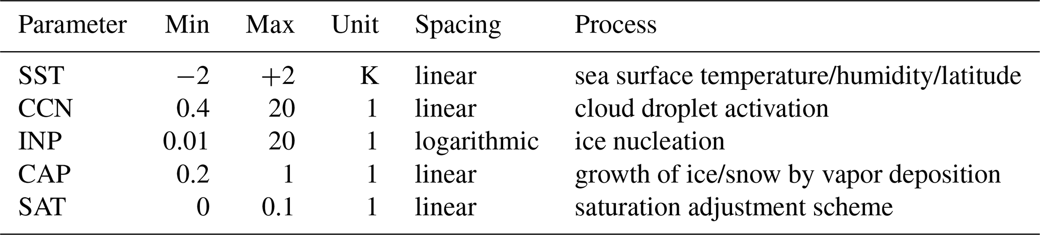
In this section we provide an overview of the properties of WCB trajectories at the end of ascent, since this is where we focus most of our analysis. Spatially, the end of the ascent is spread across a large area, ranging in longitude from 60° W to more than 45° E (Fig. 2c). However, the core of end-of-ascent longitude positions are focused around 60 to 10° W (Fig. 2a) with only very few extending further east. In latitude, trajectories finish their ascent between 35 and 85° N (Fig. 2c), with largest density at approximately 40, 50, 58 and 68° N (Fig. 2b), indicating the presence of large-scale organization in the ascent of air within the WCB. For the discussion of changes in the positions of WCB trajectories with parameter perturbations, the reader is directed to Oertel et al. (2025), since this is not the area of focus in this study.

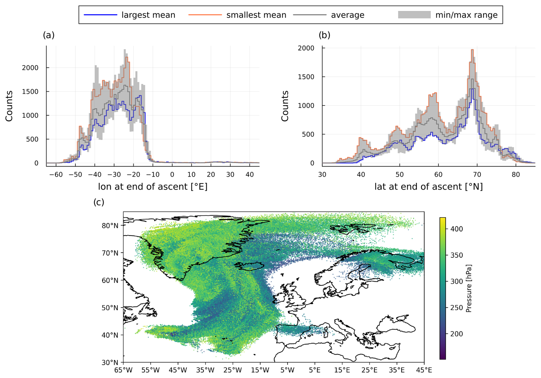
Figure 2 Histograms for (a) longitude and (b) latitude at the end of ascent, with each showing distributions for PPE members with the largest mean (blue) and smallest mean (orange), as well as the average distribution in grey and the min/max distributions per variable bin in the shaded area. Panel (c) shows the trajectory positions at the end of the ascent for all PPE members (note that trajectories finish their ascent at different times in the simulation), with pressure as the color scale.

At the end of ascent, trajectories across all PPE members ascend to pressures between approximately 200 and 400 hPa (Fig. 3c and d). Temperatures range from approximately −60 to −30 °C; the majority of trajectories (ca. 75 %) have temperatures below the homogeneous freezing temperature of −38 °C (Fig. 3a and b). Trajectories are very dry when they complete their ascent, with an average $q_{\mathrm{v}}^{\mathrm{mean}}$ of 0.23 g kg⁻¹ (Fig. 3e and f). However, the distribution of q_v in each PPE member is skewed towards higher values, meaning that although the median q_v at the end of ascent ranges from 0.17 to 0.20 g kg⁻¹ for PPE members, all PPE members also have (few) trajectories with q_v larger than 0.6 g kg⁻¹ at end of ascent. We discuss the effects of parameter perturbations on T, p and q_v in Sect. 3.1.

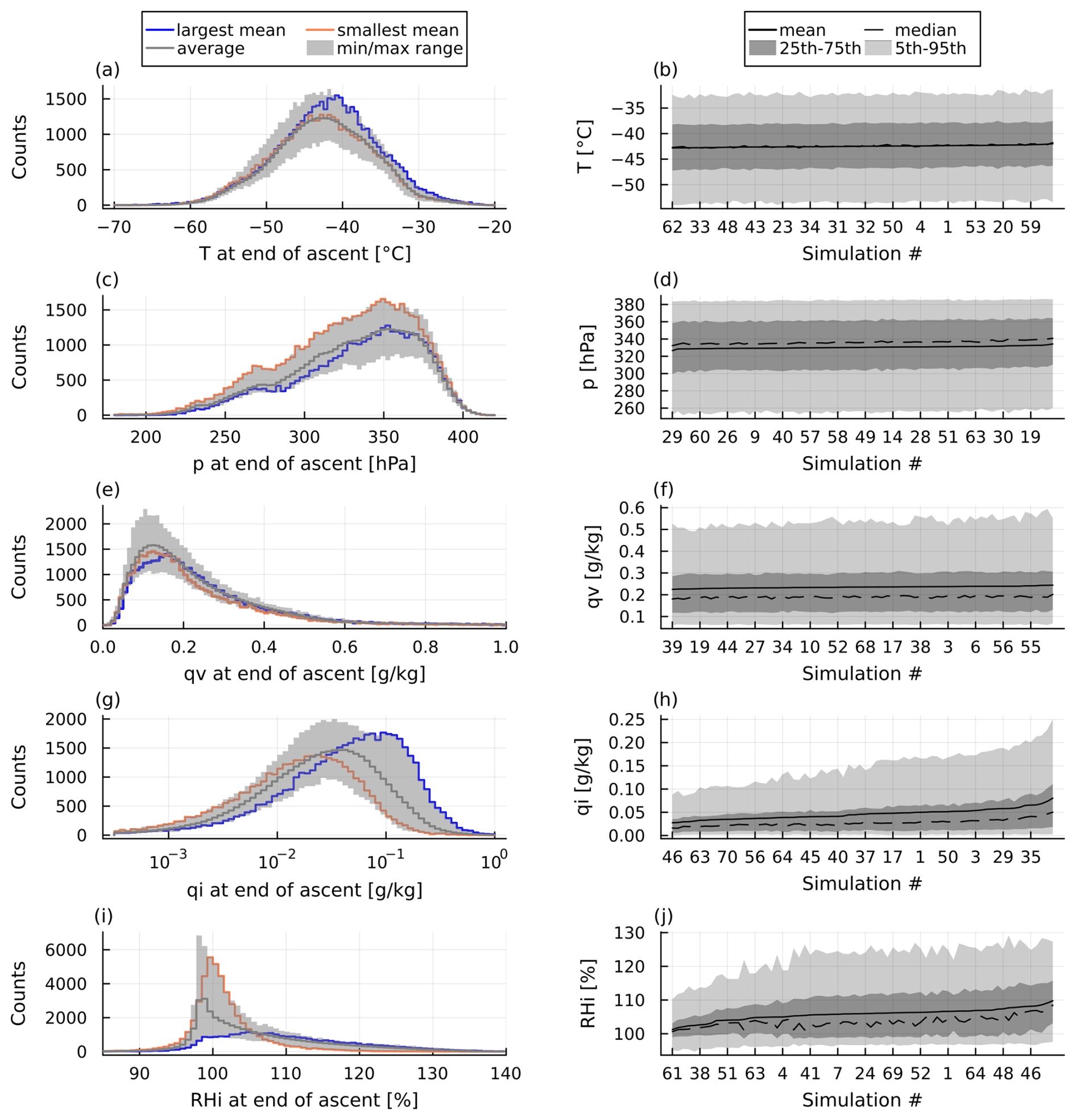
Figure 3 Histograms for (a) temperature T, (c) pressure p, (e) specific humidity q_v, (g) ice mass mixing ratio q_i (note the logarithmic x-axis) and (i) relative humidity over ice RH_i at the end of ascent. Each figure shows distributions for PPE members with the largest mean (blue) and smallest mean (orange) of the respective variable being depicted, as well as the average distribution in grey and the min/max distributions per variable bin in the shaded area. Panels (b), (d), (f), (h) and (j) show T^mean, p^mean, $q_{\mathrm{v}}^{\mathrm{mean}}$, $q_{\mathrm{i}}^{\mathrm{mean}}$ and ${\mathrm{RH}}_{\mathrm{i}}^{\mathrm{mean}}$ per PPE member, respectively, sorted according to the mean, with 5th to 95th percentiles and inter-quartile range shaded in grey.

Almost all trajectories are fully glaciated by the end of their ascent and less than 1 % of all trajectories have cloud droplet mass mixing ratio (q_c) larger than zero (not shown). Trajectories at end of ascent also contain no graupel and no rain (not shown). The only relevant hydrometeor species are therefore ice and snow, with the former being the most predominant (with ice mass mass mixing ratio $q_{\mathrm{i}}^{\mathrm{mean}}$ and ice number mixing ratio $N_{\mathrm{i}}^{\mathrm{mean}}$ being on average 0.046 g kg⁻¹ and 2.49×10⁶ kg⁻¹, compared to $q_{\mathrm{s}}^{\mathrm{mean}}$ and $N_{\mathrm{s}}^{\mathrm{mean}}$ which are on average 0.001 g kg⁻¹ and 540 kg⁻¹). We therefore focus our analysis on q_i at the end of ascent, which shows a peak at small values close to ∼0.05 g kg⁻¹ and a long tail to larger values of up to around 0.3 g kg⁻¹ for the PPE member with the highest mean q_i (Fig. 3g). Hydrometeor contents are therefore roughly one order of magnitude smaller than q_v. In contrast to q_v, we find that q_i varies much more strongly between PPE members (Fig. 3g and h). The standard deviation of $q_{\mathrm{i}}^{\mathrm{mean}}$ across all PPE members is 0.01 g kg⁻¹ (vs. 0.004 g kg⁻¹ for $q_{\mathrm{v}}^{\mathrm{mean}}$) and the highest $q_{\mathrm{i}}^{\mathrm{mean}}$ (0.080 g kg⁻¹) is almost 3 times larger than the smallest $q_{\mathrm{i}}^{\mathrm{mean}}$ (0.027 g kg⁻¹). This corroborates the visual impression from Fig. 3h of substantial changes in the q_i distribution in particular with respect to the occurrence of high q_i values. We assess the effects of parameter perturbations on the hydrometeor content at the end of ascent in Sect. 3.2.

The mean relative humidity over ice (RH_i) for all PPE members is larger than 100 % (Fig. 3j), but also here we find much stronger differences between PPE members (Fig. 3i and j) than for T, p and q_v, which is particularly interesting because the differences in q_v are small. The smallest RH${}_{\mathrm{i}}^{\mathrm{mean}}$ of 101.2 % is not only much smaller than the largest (109.8 %), but the two distributions are also markedly different (Fig. 3i): The RH_i distribution from the PPE member with the smallest RH${}_{\mathrm{i}}^{\mathrm{mean}}$ is relatively narrow with only few trajectories exceeding 110 % RH_i, while the distribution from the PPE member with the largest RH${}_{\mathrm{i}}^{\mathrm{mean}}$ is very broad featuring RH_i values above 110 % (120 %) in 44 % (15 %) of the trajectories. We interpret the effects of parameter perturbations on the relative humidity at the end of ascent in Sect. 3.3.

3.1 Parameter effects on temperature, pressure and specific humidity at the end of ascent

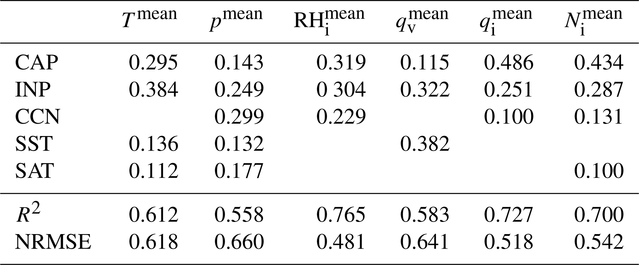
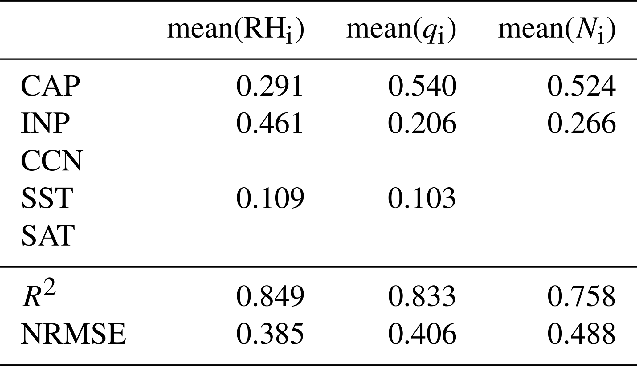
As discussed above, T, p and q_v show little variation between PPE members (Fig. 3b, d and f), with the variability within each PPE member being significantly larger than the mean differences between PPE members. The distributions for PPE members with the highest and smallest mean values for T, p and q_v are also very similar (Fig. 3a, c and e). The relatively large spread of the distribution (min/max shaded areas in Fig. 3a, c, and e) is a result of the differing number of WCB trajectories per PPE member (which is primarily controlled by SST, see Oertel et al., 2025). The RF${}_{\mathrm{mean}\left(p\right)}^{\mathrm{2}}$ and RF${}_{\mathrm{mean}\left(T\right)}^{\mathrm{2}}$ model predictions (which we use to determine which parameters have the strongest influence on a variable, as long as the model prediction is strong) are also relatively weak, with mediocre R² and large NRMSE-values (Table 2). Therefore, the RF model does not find meaningful changes in T^mean, p^mean and $q_{\mathrm{v}}^{\mathrm{mean}}$ with parameter perturbations. We interpret this inability of the parameters to change the pressure, temperature, and vapor conditions at the end of the WCB ascent as an indication that the thermodynamic conditions in the outflow of a WCB are largely constrained.

Table 2 Impurity-based feature importance (IBF) scores of CAP, INP, CCN, SST and SAT derived from RF${}_X^{\mathrm{1}}$ for a selection of mean variables. Only scores ≥0.1 are included. The bottom rows show the R² and NRMSE value for the predictions of the second iteration of the forest regression model (RF${}_X^{\mathrm{2}}$) using only parameters with IBF ≥ 0.1. Note: all of these values are slightly different each time a forest model regression is performed; the values shown here are averaged over 100 iterations.

However, some relationships are worth noting. For example, T^95th and $q_{\mathrm{v}}^{\mathrm{95}\mathrm{th}}$ show an unmistakable correlation with SST perturbations (Fig. A1c in the Appendix) and to each other (Fig. A1a). Oertel et al. (2025) found that increasing SST leads to higher potential temperatures and a greater number of WCB trajectories, as enhanced latent heat release facilitates more cross-isentropic ascent. Consequently, in PPE members with higher SST, more trajectories are able to meet the 600 hPa ascent threshold that would otherwise fall short at lower SST values. We therefore attribute the increase in T^95th and $q_{\mathrm{v}}^{\mathrm{95}\mathrm{th}}$ with SST to the larger number of WCB trajectories that end their ascent at relatively high pressures (∼ 400 hPa) and lower latitudes (∼ 40° N) in high-SST simulations (not shown). Trajectories that fall short of the 600 hPa threshold are more likely to be absent from the WCB trajectory set in PPE members with lower SST.

An important finding from a previous analysis of q_v in WCB outflow by Schwenk and Miltenberger (2024) was that q_v values are largely controlled by temperature. We find the same in the present PPE: the specific humidity for the ensemble members with the highest and lowest $q_{\mathrm{v}}^{\mathrm{95}\mathrm{th}}$ values correlates strongly with the calculated saturation specific humidity (using parcel temperature T and pressure p, Fig. A1b; R_s≈0.99 for both). This strong correlation indicates that in both PPE members the specific humidity at the end of ascent is predominantly constrained by the thermodynamic conditions, i.e., changes in q_v are a result of changes in temperature.

In summary, the parameter perturbations in our PPE only have a limited effect on changing the distributions of T, p and q_v at the end of ascent, indicating that the conditions at the end of ascent experience strong thermodynamic constraints.

3.2 Effect of parameter perturbations on the hydrometeor content (during and at the end of the ascent)

At the end of ascent, virtually all hydrometeors are ice (Sect. 3). The summary statistics as well as distributions of mass mixing ratios q_i show large differences between PPE members (Fig. 3g and h) suggesting that the parameter perturbations influence the hydrometeor content in the outflow of the WCB. The IBF scores (Table 2) indicate that CAP and INP scaling factors are the most important parameters for the mean ice number (N_i) and mass (q_i) mixing ratio. The CCN scaling factor shows an IBF score of approximately 0.1 for these variables, indicating that it is less important in the ice-phase than it is in the liquid-phase and mixed-phase cloud regime (as is shown later in this section).

3.2.1 Impact of CAP on ice properties at end of ascent

Increasing CAP clearly decreases $q_{\mathrm{i}}^{\mathrm{median}}$ at the end of the ascent while the spread in values remains largely unaltered (Fig. 4a, note logarithmic y-axis). The spread (in the percentiles) is mostly unchanged because the distribution and shape of q_i values remains similar for large and small CAP (Fig. 4d). Increasing CAP also strongly decreases $N_{\mathrm{i}}^{\mathrm{median}}$ at the end of the ascent (Fig. 4b) and reduces the spread; the simulations with the largest and smallest values for CAP have standard deviations for log ₁₀(N_i) of 0.54 and 1.01, respectively. This decrease in N_i and spread is a result of a large difference in the distribution shape of N_i values for PPE members with large and small CAP (Fig. 4e). When CAP is small (<0.4) the distribution of N_i shows a large spread and hints at bi-modality, with one peak (or mode) at approximately 10⁵ kg⁻¹ and a second mode at approximately 5×10⁶ kg⁻¹. When CAP is large (≥0.8) the bi-modality almost disappears, reducing the spread. Additionally, the peak of the distribution shifts to smaller N_i for PPE members with larger CAP. The radius r_i, on the other hand, increases clearly with CAP, as does the spread (Fig. 4c and f).

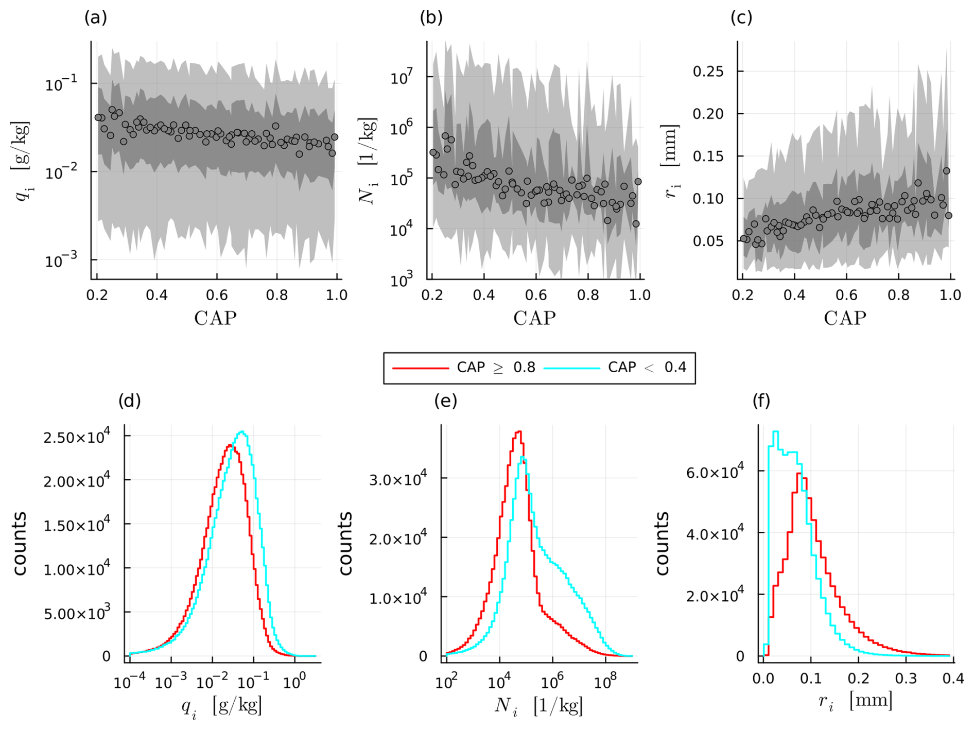
Figure 4 (a) q_i, (b) N_i and (c) ice radius (r_i) at the end of the ascent over CAP, with makers showing median values and shaded areas the 5th to 95th percentiles (light grey) and 25th to 75th percentiles (dark grey). Panels (d), (e), and (f) show q_i, N_i and r_i at the end of the ascent respectively, but as histograms for all PPE members with CAP values either larger than 0.8 (red; in total 16 PPE members and 633 400 trajectories) or smaller than 0.4 (cyan; in total 18 PPE members and 696 846 trajectories).

We interpret these findings as follows: An increase in CAP enhances the deposition rate, which, in the mixed-phase, can accelerate the Wegener–Bergeron–Findeisen (WBF) process. Consequently, when CAP is high, ice crystals grow more rapidly, depleting vapor more efficiently and accelerating the evaporation of cloud droplets. This leads to an earlier onset of full glaciation (see the Supplement, Fig. S1) – defined as the first time step when q_c reaches zero – at higher pressures and temperatures. Thus, fewer cloud droplets reach the homogeneous-freezing level of −38 °C, where they would otherwise freeze and generate numerous small ice crystals. This hypothesis is supported by the fact that the only physical process producing ice-crystal number mixing ratios in the order of 10⁷–10⁸ kg⁻¹ is homogeneous cloud freezing. Heterogeneously produced ice-crystal number mixing ratios cannot exceed the number of INPs, which is on the order of 10⁴ kg⁻¹. More homogeneously freezing cloud droplets when CAP is low explains why the distribution appears slightly bi-modal at low CAP values – indicating that a large proportion of trajectories contain small cloud droplets that reach the homogeneous-freezing level – but becomes uni-modal at high CAP values. Furthermore, an increased deposition rate leads to the formation of larger ice crystals (reflected in the increase of r_i with CAP), which have higher terminal velocities and precipitate more quickly. This precipitation process reduces the peak number mixing ratio of ice crystals N_i and, ultimately, the ice mass mixing ratio q_i.

3.2.2 Impact of INP on ice properties at end of ascent

The effects of varying the INP scaling factor exhibit similarities to those observed for CAP, but with some notable differences. As for CAP, an increase in the INP scaling factor leads to a decrease in $q_{\mathrm{i}}^{\mathrm{median}}$, albeit to a lesser extent than CAP (Fig. 5a). Similarly to CAP, low INP scaling factor values result in a distribution of N_i that is slightly bi-modal with a high spread, and high values result in a uni-modal distribution with a low spread (Fig. 5b). However, the key difference is that the peak of the N_i distribution shifts in the opposite direction, i.e. towards smaller N_i values with an increase in INP scaling factor (Figs. 5e, S2). Although the INP scaling factor has a stronger effect on the location of the peak N_i than CAP (Fig. S2), it shows no clear relationship with $N_{\mathrm{i}}^{\mathrm{median}}$ values (Fig. 5b) because the spread of values is much larger and, due to the exponential nature of N_i-values, this means that the peak does not correspond to the mean. The peak for r_i shifts to smaller r_i values with a decrease in INP scaling factor, (Fig. 5f), but the spread is larger which is why this trend is less apparent in $r_{\mathrm{i}}^{\mathrm{median}}$ (Fig. 5c).

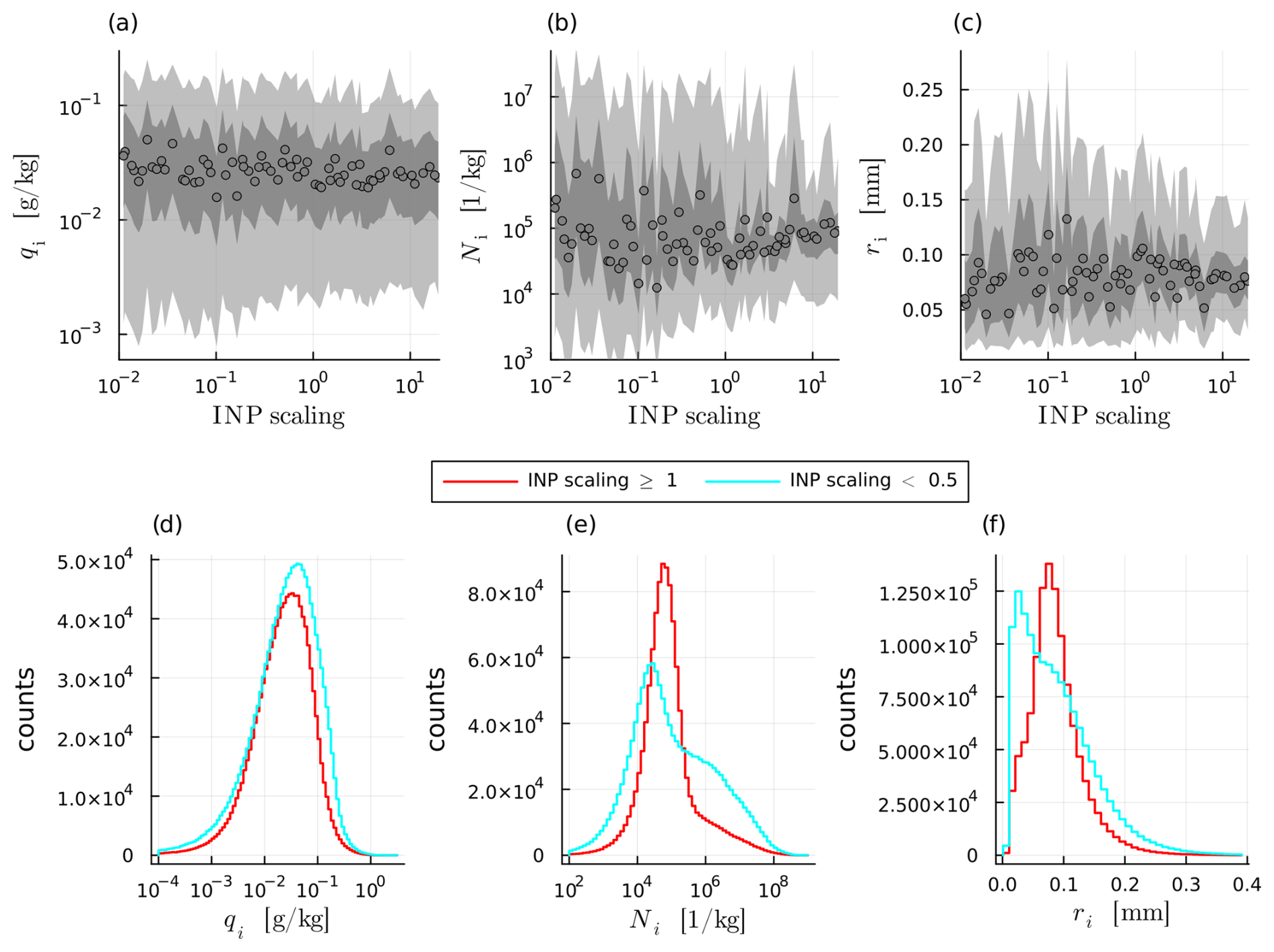
Figure 5 (a) q_i, (b) N_i and (c) ice radius (r_i), over INP, with makers showing median values and shaded areas the 5th to 95th percentiles (light grey) and 25th to 75th percentiles (dark grey). Panels (d), (e), and (f) show q_i, N_i and r_i respectively, but as histograms for all PPE members with INP scaling factors either larger than 1 (red; in total 29 PPE members and 1 123 557 trajectories) or smaller than 0.5 (cyan; in total 35 PPE members and 1 417 123 trajectories).

We interpret these findings as follows: By design, increasing the INP scaling factor enhances the immersion freezing of cloud droplets, the deposition nucleation of ice, and the freezing of raindrops (Sect. 2), thereby accelerating the conversion of cloud droplets to ice. Similarly to CAP, a higher INP scaling factor leads to an earlier onset of full glaciation (see Fig. S1) with fewer cloud droplets reaching the homogeneous-freezing level, where they would otherwise form numerous small ice crystals. The explanation for the bi-modal distribution of N_i at low INP scaling factor values and the transition to a uni-modal distribution at higher values is therefore the same as for CAP. The only addition is that a smaller INP scaling factor shifts the location of the peak N_i to smaller values (a smaller CAP shifts it to larger values) and also exerts a stronger control on it (Fig. S2). If this peak is interpreted as those trajectories that encounter no (or less) homogeneous freezing of cloud droplets, then its location should primarily increase with INP scaling, which is what we observe. Furthermore, since hydrometeor growth by deposition is more efficient than by condensation, and a higher INP scaling factor prolongs the duration spent in the ice phase, a higher INP scaling factor ultimately promotes the formation of larger ice crystals, contributing to the observed increase in r_i and the slight decrease in q_i (heavier ice particles fall out more quickly). The tail towards larger r_i for small INP can be explained by the fact that when fewer ice crystals form during the ascent, there is less competition for available vapor, allowing for individual ice crystals to grow larger. This also enhances the conversion from ice to snow, which is supported by the fact that on average, q_s at the end of the ascent slightly increases when INP is small (not shown).

3.2.3 Impact of CCN on ice properties during the ascent

The third most important parameter (based on the IBF scores, Table 2) for the ice content at the end of the ascent is CCN. However, the CCN scaling factor primarily influences the hydrometeor content and mixed-phase microphysics during the WCB ascent as opposed to at the end. It correlates almost perfectly with the mean of maximum number mixing ratio of hydrometeors achieved during the ascent (R_s=0.9994, Fig. 6d). This clear dependency comes from the fact that an increase in the CCN scaling factor primarily increases the number of cloud droplets and reduces the number of rain drops during the ascent (Fig. 6e). With an increase in CCN, cloud droplets during the ascent become smaller; for simulations with the largest and smallest CCN scaling factor, the mean cloud droplet mass is approximately $\mathrm{72}\times {\mathrm{10}}^{-\mathrm{9}}$ and $\mathrm{9}\times {\mathrm{10}}^{-\mathrm{9}}$ g, respectively. Smaller cloud droplets delay the formation of rain and enhance the residence time of liquid condensate. This delay is the reason why air parcels begin their glaciation (defined as first time when ($q_{\mathrm{c}}+q_{\mathrm{r}}/q_{\mathrm{tot}})<\mathrm{0.5}$) at lower pressures and temperatures (i.e., later in the ascent) when the CCN scaling factor is larger (Fig. 6a and b). This in turn leads to a larger mean of the maximum mixing ratios of supercooled liquid water (max(SLW)) achieved during the ascent with an increasing CCN scaling factor (Fig. 6c).

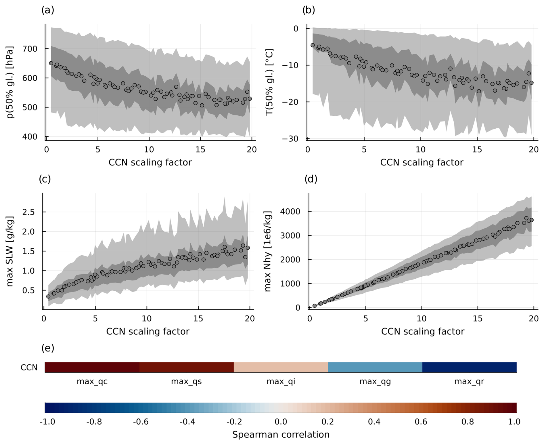
Figure 6 Scatter plots of (a) mean pressure at 50 % glaciation ($(q_{\mathrm{i}}+q_{\mathrm{s}}+q_{\mathrm{g}})/q_{\mathrm{tot}}=\mathrm{0.5}$), (b) mean temperature at 50 % glaciation, (c) mean of maximum total hydrometeor mass mixing ratio during the ascent and (d) mean of maximum total hydrometeor number mixing ratio during the ascent over CCN scaling factors. Shaded areas show 5th to 95th percentiles (light grey) and 25th to 75th percentiles (dark grey). Spearman correlation coefficients for CCN scaling factors with individual mean of the maximum mass mixing ratios during the ascent for all hydrometeors are shown in (e).

The mean of the maximum mixing ratio for snow (max(q_s)) during ascent also increases with CCN, while for graupel (max(q_g)) it decreases (Fig. 6e). We explain this as follows: increased CCN concentrations lead to more numerous but smaller cloud droplets, which slows the formation of raindrops. This, in turn, reduces the collision efficiency between ice or snow particles and cloud droplets, slowing the (continuous) conversion to graupel. As a result, snow remains more abundant and graupel less abundant. However, this large effect of the CCN scaling factor on the hydrometeor population during the ascent is mostly lost by the end of the ascent, showing that once air parcels glaciate, CAP and INP dominate the ice-phase cloud microphysics.

3.2.4 (Non-)Impact of SST on ice properties

Another important result from the analysis of parameter effects on the hydrometeor population is that changes to SST, which substantially increase the amount of WCB trajectories that ascend quickly (Oertel et al., 2025), show no effect on distributions of N_i and q_i at the end of ascent. This absent effect is surprising, because Schwenk and Miltenberger (2024) found that fast ascending trajectories (τ₆₀₀<5 h) have a larger hydrometeor content at the end of the ascent than more slowly ascending trajectories (τ₆₀₀>20 h). Given that in the WCB case from this Paper, higher SSTs shorten ascent timescales and enhance convective activity (Oertel et al., 2025), we would have expected N_i and q_i to increase for simulations with higher SST. However, our findings indicates that the impact of CAP and INP dominates. A likely reason is that the WCB we examine is only weakly convective: only 5 % of trajectories have τ₆₀₀<10 h, and that fraction changes only slightly across the SST ensemble (4.5 % at −1 °C, 6.4 % at +1 °C). With so few strongly convective parcels, SST-induced changes in vertical motion leave little imprint on N_i and q_i. We therefore hypothesize that, in a more convectively active WCB, an identical SST perturbation would produce a larger change in the convective fraction and, consequently, a clearer SST impact on N_i and q_i. Finally, we emphasize that changes in SST have no apparent effect on the temperature and pressure at which air parcels glaciate (see Fig. S7).

3.3 Effect of parameter perturbations on relative humidity over ice (RH_i) at end of ascent

Despite the strong temperature control on q_v values (Sect. 3.1), previous work suggests that substantial supersaturation over ice (up to 120 %) can exist in WCB outflow (Schwenk and Miltenberger, 2024; Spichtinger et al., 2005). In the PPE, we also find large RH_i values as well as a strong variability in RH_i distributions between PPE members (Fig. 3i and j). The parameters with the largest IBF scores (Table 2) for mean RH_i are CAP (0.319), INP (0.304) and CCN (0.229), and the RF${}_{\mathrm{mean}\left({\mathrm{RH}}_{\mathrm{i}}\right)}^{\mathrm{2}}$ model has a good predictive capability, with R²=0.765 and NRMSE = 0.481. The PDPs show that increases in CAP, INP and CCN all work to decrease RH_i (see Fig. S3). The two-dimensional PDPs (Fig. 7) additionally indicate that these parameters have a joint impact: an increase in CAP, INP and CCN is most effective in reducing RH${}_{\mathrm{i}}^{\mathrm{mean}}$ when the respective other two parameters are also increasing (lowest RH${}_{\mathrm{i}}^{\mathrm{mean}}$ values seen only in top-right corners of Fig. 7). Notably, these relationships seem non-linear when CAP, INP scaling and CCN scaling are particularly low or high, indicating that the distribution of these parameter values in the real-world are important for determining whether the overall sensitivity of RH_i to perturbations is large or small.

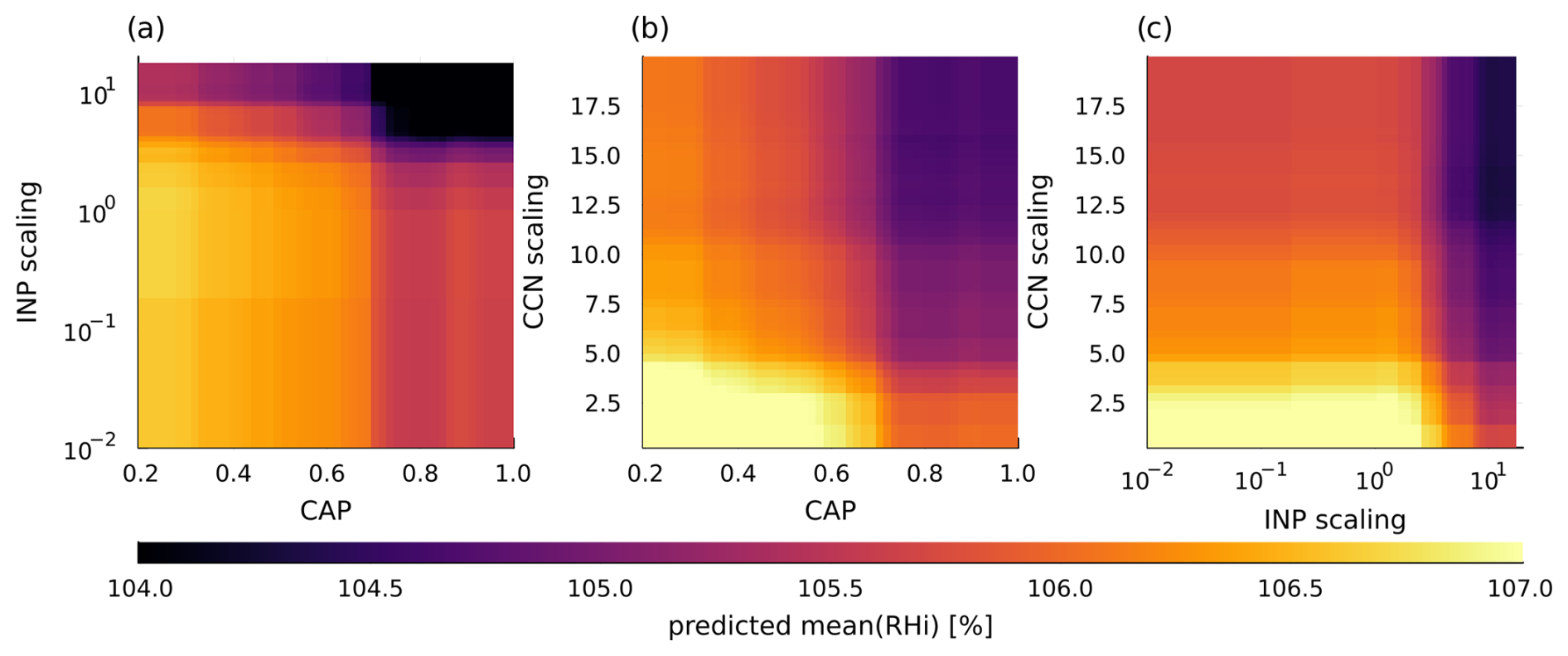
Figure 7 Two dimensional PDPs for RF${}_{\mathrm{mean}\left({\mathrm{RH}}_{\mathrm{i}}\right)}^{\mathrm{2}}$ for INP vs. CAP in (a), CCN vs. CAP in (b) and CCN vs. INP in (c).

However, when considering the median RH_i values instead of the mean, the joint impacts of parameter perturbations turn out to be more nuanced. An increase in CAP values only reduces the median RH_i when the INP scaling factor is larger than one (red dots in Fig. 8a, $R_{\mathrm{s}}=-\mathrm{0.72}$). When the INP scaling factor is smaller than one, an increase in CAP slightly increases the median RH_i, but the correlation is weak (cyan dots in Fig. 8a, R_s=0.1). The same is true the other way around: an increase in INP scaling factor increases the median RH_i when CAP is smaller than 0.5 (cyan dots in Fig. 8b, R_s=0.66) and only shows a slight decrease in median RH_i when CAP is larger than 0.5 (red dots in Fig. 8b, $R_{\mathrm{s}}=-\mathrm{0.28}$). We also find that the spread of RH_i values reduces strongly with an increase in CAP and INP (shaded areas in Fig. 8a and b). The simulations with the smallest CAP and INP scaling have standard deviations in RH_i of 10.8 % and 9.8 %, and for the largest CAP and INP scaling this drops to 5.6 % and 6.8 %. This behavior is not seen for the CCN scaling factor, which reduces the median RH_i regardless of CAP and INP scaling and does not influence the spread (standard deviation of RH_i≈9 % for simulations with the largest and smallest CCN scaling; Fig. 8c). The fact that the mean, median and spread of RH_i values are all influenced differently by perturbations of the INP scaling factor and CAP is a strong indication that these parameters and their combination change the distribution of RH_i values between different PPE members.

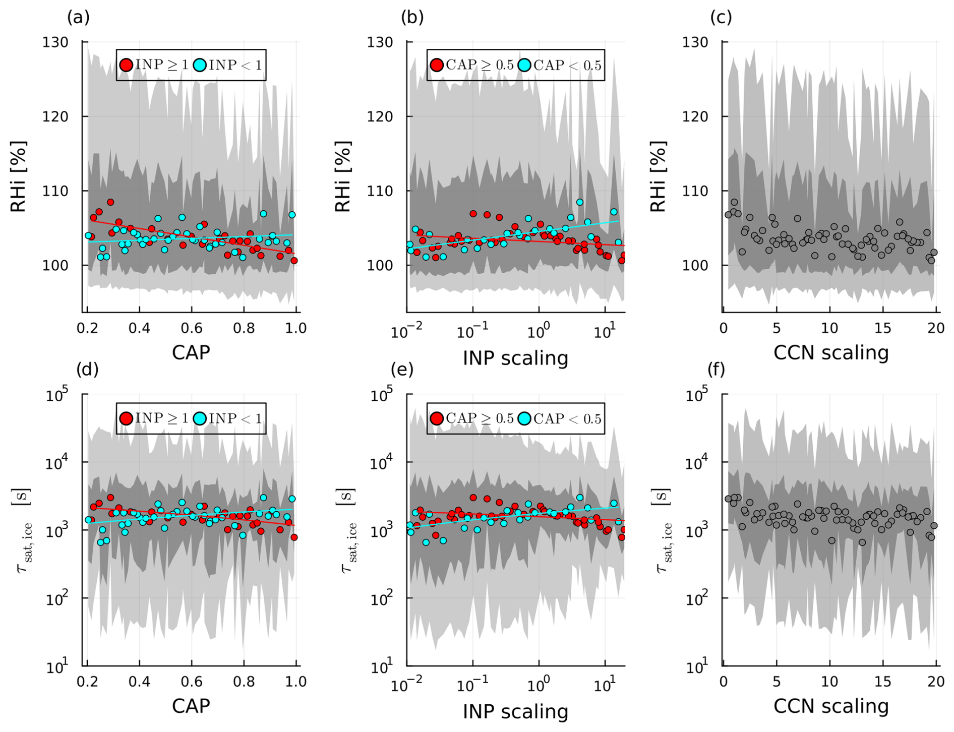
Figure 8 Scatter plots of RH${}_{\mathrm{i}}^{\mathrm{median}}$ over CAP (a), INP (b) and CCN (c) perturbations, with 25th–75th percentile range shaded in dark grey and 5th–95th percentile range shaded in light grey. Cyan and red points are masked according to INP in (a) and CAP in (b), with lines indicating a linear fit (can seem curved due to logarithmic axes) through the corresponding colored data points. The same in (d), (e) and (f) except for mean τ_sat,ice.

Indeed, we find that RH_i distributions in PPE members with both large INP scaling factors and large CAP differ strongly from those with low values of both parameters (Fig. 9a). When accumulating PPE members where both CAP > 0.8 and the INP scaling factor > 1 (red histogram in Fig. 9a), we find a RH_i distribution that peaks at approximately RH_i=100 % and is slightly skewed to larger values (tapers off at around RH_i=120 %). However, the distribution of RH_i in PPE members with CAP < 0.4 and an INP scaling factor < 0.5 (cyan histogram in Fig. 9b) has a much sharper peak at RH_i slightly below 100 % and a much larger tail to large RH_i of 135 % and more. The mean and median RH_i for the first group (CAP and INP scaling large) are both approximately 103 %, whereas for the second group (CAP and INP scaling small), the mean RH_i of 106 % is larger than the median RH_i of 103 %. This explains both the differing behaviors of the mean and median RH_i with CAP and INP as well as the spread, which increases with the asymmetry of the distribution. We note that the peak RH_i for small CAP and INP indicates that most trajectories in those PPE members are subsaturated at the end of the ascent. As we will see in Sect. 5, ice crystals sublimate in the outflow because of this subsaturation.

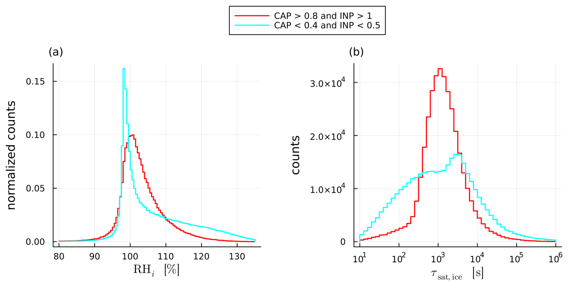
Figure 9 Histograms for (a) RH_i and (b) τ_sat,ice at the end of the ascent for all PPE members with CAP > 0.8 and INP scaling factor > 1 (red; in total 9 PPE members and 357 888 trajectories) or CAP < 0.4 and INP scaling factor < 0.5 (cyan; in total 9 PPE members and 363 512 trajectories).

Before interpreting these findings, it is essential to note that in the ICON model, supersaturation with respect to water can only develop when an air parcel is fully glaciated, as this is the point at which the saturation adjustment scheme, which enforces relative humidity over water of 100 %, becomes inactive. Consequently, when examining the effects of parameter perturbations on RH_i at the end of ascent, it is important to focus on the timing of the air parcel's full glaciation, as well as the cloud microphysical evolution after this point, since only when there is no more liquid water will we see deviations from RH_w=100 %. Note that RH_w=100 % also constrains RH_i to a temperature dependent but otherwise fixed value (with RH_i>100 %). For a fully glaciated air parcel, the relaxation timescale for supersaturation over ice (at a vertical velocity w=0 m s⁻¹) is inversely proportional to the product of ice number concentration and ice particle radius (e.g. Khvorostyanov, 1995; Khvorostyanov and Sassen, 1998; Khvorostyanov et al., 2001):

$$\begin{array}{}\text{(2)}& {\mathit{\tau }}_{\mathrm{sat},\mathrm{ice}}={\displaystyle \frac{\mathrm{1}}{\mathrm{4}\mathit{\pi }\cdot \mathrm{CAP}\cdot N_{\mathrm{i}}\cdot r_{\mathrm{i}}\cdot D_{\mathrm{v}}}}\left(\mathrm{with}\right[N_{\mathrm{i}}]={\mathrm{m}}^{-\mathrm{3}}),\end{array}$$

with D_v the water vapor diffusion coefficient (taken as a constant value of $\mathrm{3}\times {\mathrm{10}}^{-\mathrm{5}}$ m² s⁻¹). Equation (2) shows that parameter perturbations that lead to higher N_i and r_i should lead to a faster reduction of supersaturation over ice, and therefore, given a similar vertical velocity distribution, on average smaller RH_i. This assumption is verified by the two-dimensional histogram of all RH_i and τ_sat,ice values (taken at the end of the ascent, because w must be approximately 0) from the PPE (Fig. 10). It reveals that when τ_sat,ice is smaller than approximately 5×10² s, RH_i values are concentrated at or slightly below approximately 100 %. Above this threshold, the mean, median and spread of RH_i per τ_sat,ice-bin increase monotonically and plateau at RH_i≈115 % when ${\mathit{\tau }}_{\mathrm{sat},\mathrm{ice}}>{\mathrm{10}}^{\mathrm{4}}$ s. The increase of RH_i past ${\mathit{\tau }}_{\mathrm{sat},\mathrm{ice}}\approx \mathrm{5}\times {\mathrm{10}}^{\mathrm{2}}$ s shows that τ_sat,ice is the primary physical control of RH_i. RH_i at the end of the ascent also does not depend on RH_i at the moment of full glaciation, when the air parcels are still ascending (see Fig. S4) which solidifies that τ_sat,ice controls RH_i at the end of the ascent. Therefore, to interpret effect of parameter perturbations on RH_i, we must first understand their effects on τ_sat,ice.

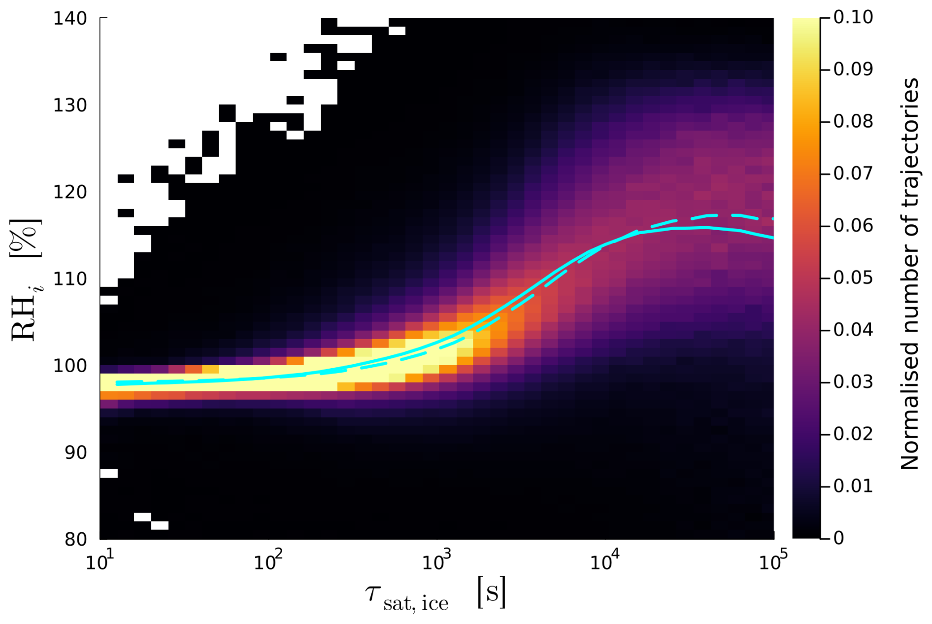
Figure 10 Two dimensional normalized histogram of RH_i over τ_sat,ice for all trajectories from all PPE members. Cyan lines show mean (solid) and median (dashed) values per τ_sat,ice-bin.

The median τ_sat,ice (Fig. 8d, e and f, note logarithmic y-axis) varies with CAP, INP and CCN parameter perturbations in a similar manner than RH_i (Fig. 8a, b and c): as indicated by the red and cyan lines in Fig. 8d and e, CAP slightly reduces τ_sat,ice when INP scaling is large ($R_{\mathrm{s}}=-\mathrm{0.57}$) and increases it when INP scaling is small (R_s=0.36); the INP scaling factor slightly reduces τ_sat,ice when CAP is large ($R_{\mathrm{s}}=-\mathrm{0.32}$) and increases it when CAP is small (R_s=0.62); and as indicated by Fig. 8f, the CCN scaling factor reduces τ_sat,ice regardless of CAP and INP scaling. As for RH_i, joint perturbations in the INP scaling factor and in CAP influence the distribution of τ_sat,ice (Fig. 9b). When CAP > 0.8 and INP scaling factor > 1 (red histogram in Fig. 9b, note the logarithmic x-axis and logarithmic spacing of bins), τ_sat,ice values peak at approximately 10³ s and fall off symmetrically to either side. On the other hand, when CAP < 0.4 and INP < 0.5 (cyan histogram in Fig. 9b) the distribution is very broad and bi-modal, with the largest peak at a larger value of approximately 5×10³ s and a second peak at a lower value of approximately 5×10² s. As discussed above, τ_sat,ice-values below 5×10² s produce almost only RH_i-values of approximately 100 % (Fig. 10). The abundance of τ_sat,ice-values below this threshold for the group with small CAP and INP scaling (cyan histogram in Fig. 9b) therefore explains the sharp peak of the RH_i distribution (cyan histogram in Fig. 9a). The larger average value for τ_sat,ice and higher abundance of values above the threshold of 5×10² s for this same group of trajectories also explains the long tail to larger RH_i (cyan histogram in Fig. 9b), since RH_i increases strongly with τ_sat,ice beyond this threshold value (Fig. 10)

The effect that the INP scaling factor and CAP have on the distribution of τ_sat,ice (and thus RH_i) can be traced back to their effect on the hydrometeor populations at the end of the ascent (see Sect. 3.2 for physical interpretation), since τ_sat,ice is inversely proportional to N_i, r_i and CAP (Eq. 2). When the INP scaling factor or CAP is small, the distribution of N_i shows a large spread (Figs. 4b and e, 5b and e) and a bulge to larger N_i. This bulge in turn creates the bulge to smaller τ_sat,ice (Fig. 9b) and ultimately the sharp peak in RH_i (Fig. 9a). In addition, the larger spread in N_i also means there is a larger abundance of smaller N_i values, which together with the smaller r_i (Figs. 4,c and f, 5c and f) explains the larger abundance of larger τ_sat,ice-values (Fig. 9b) and ultimately the long tail to larger RH_i (Fig. 9a). In contrast, when either the INP scaling factor or CAP are large, the N_i distribution becomes narrower and more symmetrical, which in turn results in similarly shaped distributions for τ_sat,ice and ultimately RH_i.

The CCN scaling factor decreases the mean and median τ_sat,ice (Fig. 8f) but does not change the overall shape and spread of the distribution (see Fig. S5). The CCN scaling factor also has no notable effect on the hydrometeor populations at the end of the ascent (not shown), however the decrease in τ_sat,ice with increasing CCN scaling (which is weaker than the effect from INP scaling or CAP) must be due to a combined effect of CCN on N_i and r_i that does not appear in our analysis (possibly due to the time resolution of output data).

4 Impact of ascent timescale on parameter sensitivity

Schwenk and Miltenberger (2024) found that fast-ascending WCB trajectories transport significantly more hydrometeors into the UTLS and undergo distinctly different cloud microphysical processes (e.g. more riming, less deposition) compared to slower-ascending ones. Additionally, they demonstrated that precipitation formation pathways in convectively influenced WCB parcels differ markedly from those in slantwise-ascending parcels. Consequently, fast ascending trajectories likely play a key role in modulating moisture transport, which raises the question of whether the effects of parameter perturbations depend on the ascent timescale. In accordance with Oertel et al. (2025), we define trajectories with τ₆₀₀<10 h as fast ascending and repeat the analysis in the proceeding sections for this subset of WCB trajectories. We only briefly summarize how conditions at the end of the ascent change with ascent time, as they are consistent with findings by Schwenk and Miltenberger (2024).

Fast ascending trajectories ascend to lower temperatures and pressures, i.e., to higher altitudes: The average across all PPE members for the mean temperature and pressure are $\sim -\mathrm{43}$ °C and ∼330 hPa, respectively. If only fast ascending trajectories are considered, these values reduce to −47 °C ∼285 hPa. On average, $q_{\mathrm{i}}^{\mathrm{mean}}$ and $N_{\mathrm{i}}^{\mathrm{mean}}$ are also much larger for fast trajectories (0.12 g kg⁻¹ and 1.6×10⁷ kg⁻¹) than for all trajectories (0.04 g kg⁻¹ and 0.2×10⁷ kg⁻¹), and the mean RH${}_{\mathrm{i}}^{\mathrm{mean}}$ at the end of ascent for fast trajectories is closer to saturation (100.5 %) than for all trajectories (105.7 %). The mean $r_{\mathrm{i}}^{\mathrm{mean}}$ is smaller for fast trajectories (0.05 mm) than for all trajectories (0.09 mm). Fast trajectories also glaciate much later (at pressures and temperatures of ∼360 hPa and ∼241 K) than all trajectories (∼485 hPa and ∼253 K, Fig. 11a and b), which is consistent with the findings from Schwenk and Miltenberger (2024).

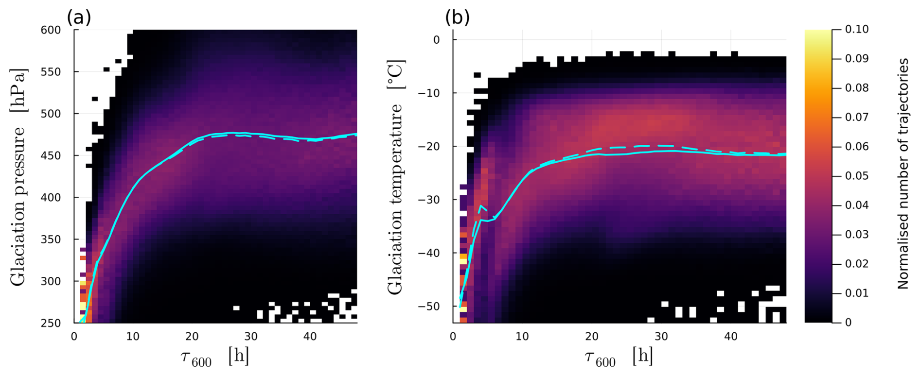
Figure 11 2-dimensional histograms of pressure in (a) and temperature in (b) at glaciation (defined as the first 60 min time step for which q_c is zero; trajectories with non-zero q_c are excluded) over the fastest 600 hPa-ascent time τ₆₀₀. Mean and median are shown by the solid and dashed line, respectively.

The effects we observed for perturbations in the INP scaling factor (Fig. 5) and CAP (Fig. 4) for all trajectories are also seen for fast ascending trajectories, only that they are much more pronounced (Fig. 12 for fast trajectories vs. Figs. 4 and 5 for all trajectories; summary statistics as in Figs. 4 and 5a, b and c are not shown). The largest effect is seen for N_i: when the INP scaling factor and/or CAP are small, the second peak towards higher N_i in the bimodal distribution becomes the largest, effectively shifting the peak N_i by two orders of magnitude (from ∼10⁵ to ∼10⁷ kg⁻¹, Fig. 12b and e). This shift means that a larger proportion of fast trajectories contain homogeneously freezing cloud droplets compared to slower ascending trajectories. This proportion increases strongly when CAP and the INP scaling factor are small.

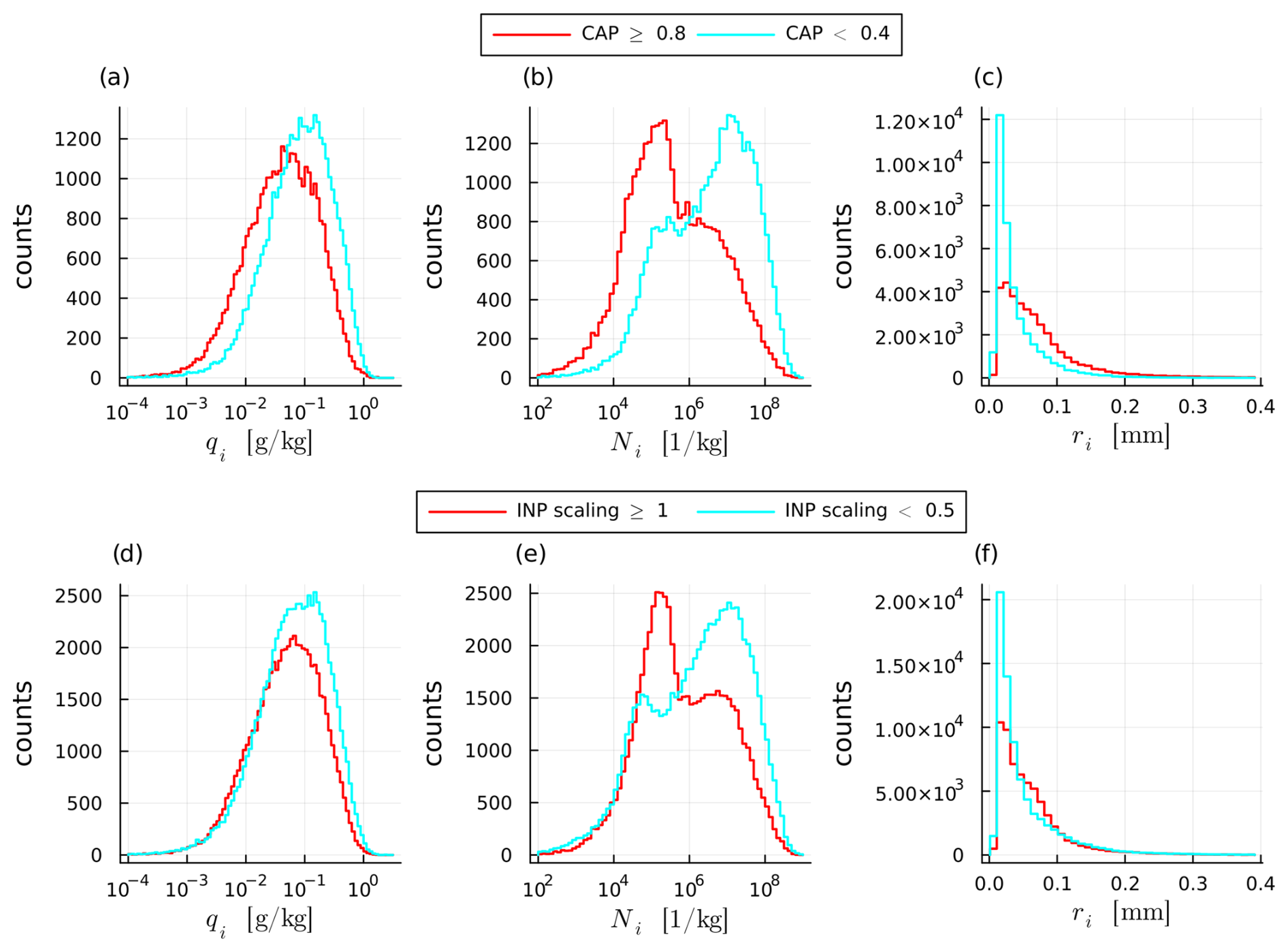
Figure 12 Histograms of q_i (a, d), N_i (b, e) and r_i (c, f) only for fast ascending trajectories and for subsets of PPE members sorted according to CAP (a–c) and the INP scaling factor (d–f).

Additionally, r_i decreases (Fig. 12c and e) and q_i increases (Fig. 12a and d) more strongly with decreasing CAP and INP for fast ascending trajectories than for all trajectories (Figs. 4f and 5f). Even though r_i is smaller for fast trajectories (which should increase τ_sat,ice), the much larger N_i-values (independent of the choice for INP scaling factor or CAP) lead to substantially smaller τ_sat,ice-values for fast ascending trajectories (compare Fig. 13b to Fig. 9b). The large shift in N_i values with INP scaling and CAP also induces a larger difference in τ_sat,ice-values for different INP scaling factors and CAP (Fig. 13b). However, the effect on the RH_i distribution (Fig. 13a) is small, because the peak τ_sat,ice for fast trajectories (Fig. 13b) is below the threshold of 5×10² s, below which RH_i stays mostly smaller than 100 % (Fig. 10), regardless of INP scaling and CAP. Therefore, fast ascending trajectories reduce ice supersaturation much faster than all trajectories due to their high ice-number mixing ratio N_i.

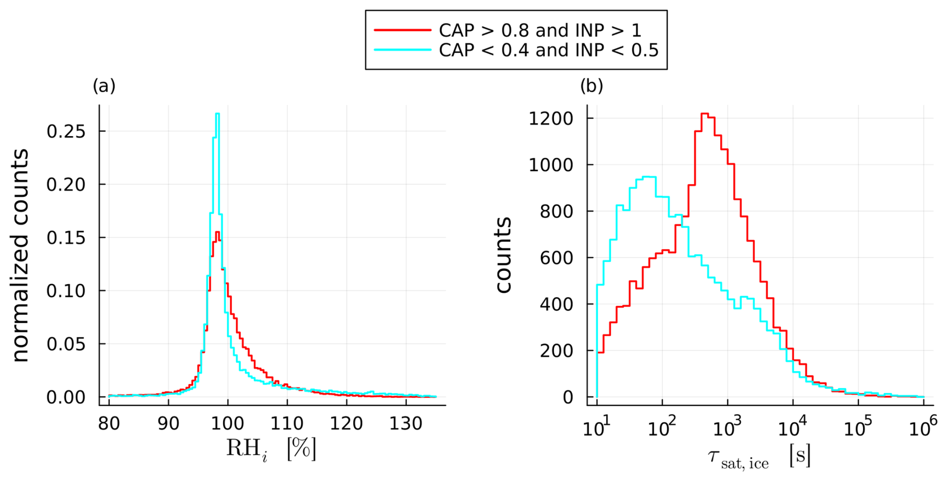
Figure 13 Histograms for (a) RH_i and (b) τ_sat,ice at the end of the ascent for only the fast ascending trajectories and PPE members with both CAP > 0.8 and INP scaling factor > 1 (red) or CAP < 0.4 and INP scaling factor < 0.5 (cyan).

We summarize that for fast ascending trajectories the INP scaling factor and CAP greatly influence the hydrometeor population at the end of the ascent, but that this has only a small effect on RH_i because large very large N_i-values lead to small τ_sat,ice in almost all cases. We also note that for fast ascending trajectories, N_i and r_i are more sensitive to CAP and the INP scaling factor than for all trajectories, suggesting that overall sensitivities to these parameters might increase for higher resolution simulations, where a greater fraction of trajectories ascend quickly.

SAT and the CCN scaling factor have very little impact on the outflow properties of the bulk of WCB trajectories, but become important when considering only the sub-set of fast ascending trajectories. SAT becomes important for the pressure, temperature and specific humidity at the end of the ascent (Fig. 14). While the distributions of these variables do not change visibly with SAT (not shown), the mean and median, as well as the upper percentiles all decrease linearly with an increase in SAT. This decrease indicates that modifications to the saturation adjustment scheme, which permit supersaturation under sufficiently high vertical velocities, can influence the thermodynamic conditions at the end of ascent when vertical velocities during the ascent are high enough. However, this effect is also a reflection of the fact that the fast ascending trajectories glaciate much later (Fig. 11), meaning that the saturation adjustment scheme is active for a longer portion of the ascent. Therefore, fast ascending trajectories spend more of their ascent at RH_w=100 %, or slightly above that value if the SAT factor is large. Thus, more vapor, that would otherwise have condensed, is transported higher into the atmosphere, resulting in a delayed latent heat release that provides some additional buoyancy later in the ascent. However, even for fast trajectories SAT still does not influence RH_i, because fast ascending trajectories are also mostly glaciated by the end of the ascent. Additionally, τ_sat,ice-values are so small, that supersaturation is quickly reduced regardless of SAT. Therefore, SAT can change the pressure and temperature at the end of the ascent for fast ascending trajectories, but is unable to modify the specific humidity values which remain constrained by the thermodynamic conditions.

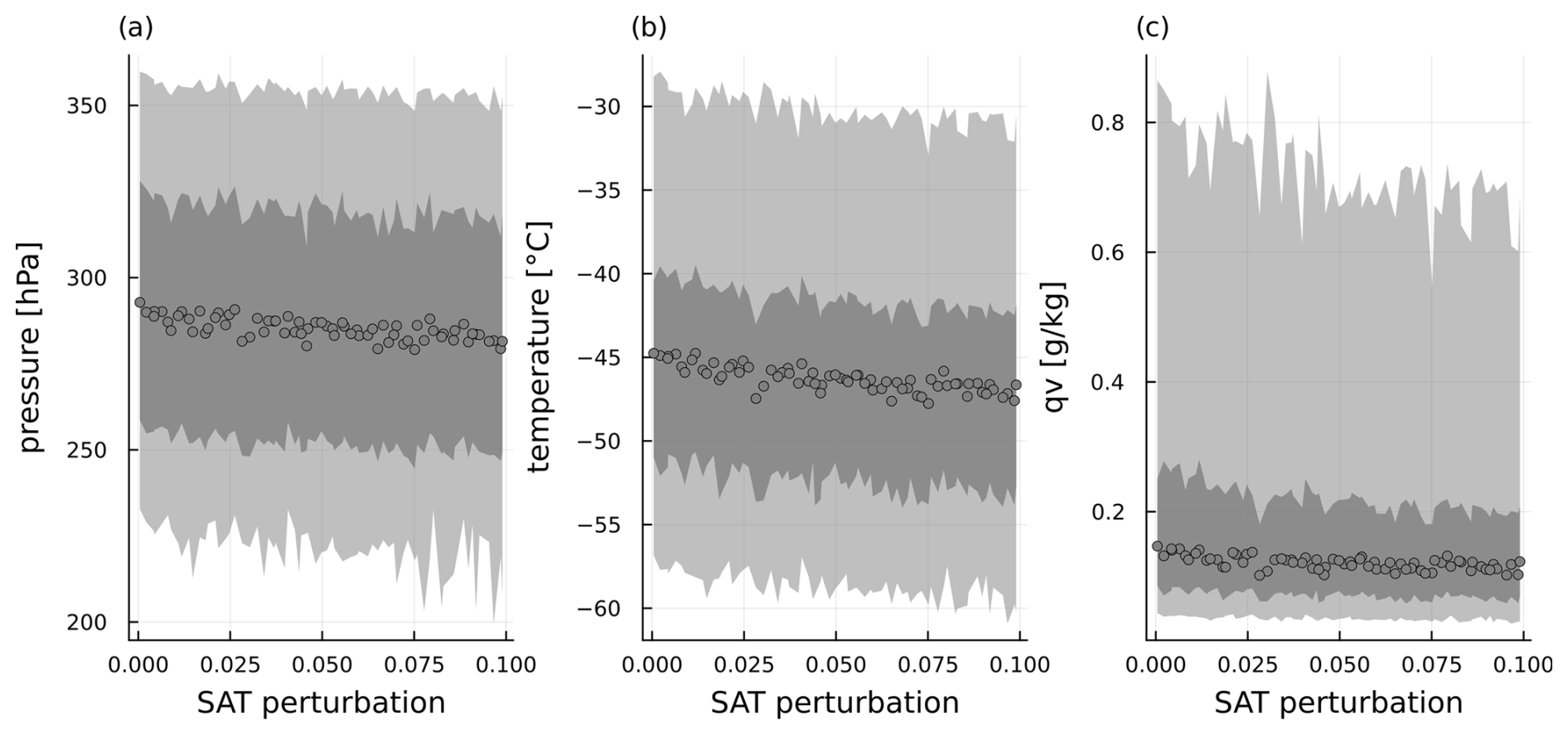
Figure 14 Pressure in (a), temperature in (b) and specific humidity q_v in (c) at the end of the ascent for only the fast ascending trajectories over the perturbation of the saturation adjustment scheme (SAT). For plots (a) and (b) the dots show the mean per PPE member, in plot (c) the dots show the median. Shaded areas indicate the inter-quartile range (dark grey) and 5th to 95th percentile (light grey).

For fast ascending trajectories, the CCN scaling factor becomes relevant for r_i, N_i, q_i, τ_sat,ice and RH_i at the end of the ascent (Fig. 15). However, the shape of distributions is only changed for N_i. The effects during the ascent are similar to those discussed in Sect. 3.2 (not shown). With an increase in CCN, the amount of cloud droplets during the ascent increases (Fig. 6d), and fast ascending trajectories have more cloud droplets that freeze homogeneously (Fig. 12b and e). Therefore, when the CCN scaling factor is large and ascent velocities are high, even more cloud droplets freeze homogeneously, decreasing r_i at the end of the ascent (Fig. 15c) and increasing N_i (Fig. 15b) as well as q_i (Fig. 15a). The orders of magnitude larger N_i and only slightly different r_i implies smaller τ_sat,ice (Eq. 2; Fig. 15c and d) and therefore smaller RH_i (Fig. 15e), which is on average 102 % when CCN scaling <5 and 99 % when CCN scaling >15. Overall, RH_i changes only slightly across PPE members for fast ascending trajectories, but among these changes, CCN scaling factor perturbations produce the largest effect. This is because for small CCN, N_i is reduced enough to produce τ_sat,ice values slightly above the threshold value of 5×10² s.

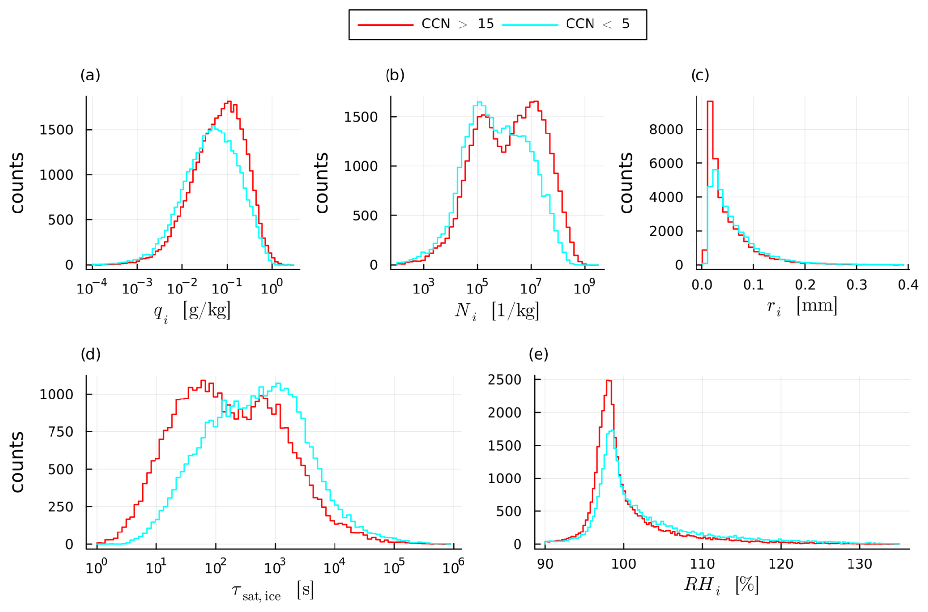
Figure 15 Histograms for q_i in (a), N_i in (b), r_i in (c), τ_sat,ice in (d) and RH_i in (e) at the end of the ascent for only the fast ascending trajectories and PPE members with a CCN scaling factor larger than 15 (red; 17 PPE members and 686 947 trajectories) or smaller than 5 (cyan; 17 PPE members and 627 912 trajectories).

5 Effects of parameter perturbations on cirrus properties 5 h after end of ascent

The conditions at the end of the ascent of a parcel likely influence but are not necessarily representative for those in the hours afterwards. Hydrometeors may precipitate out of the parcel and/or grow to reduce supersaturation (or evaporate/sublimate in case of sub-saturated conditions). RH_i values 5 h after the end of the ascent have a large spread (not shown) due to the subsidence of a large portion of trajectories (37 % of trajectories across all PPE members have a pressure at least 10 hPa higher than at the end of the ascent). We are interested in those that could retain large RH_i and therefore consider only those that have no net-descent after 5 h (∼50 % of all WCB trajectories across all PPE members). For this subset of trajectories, we consider the impact of the parameter perturbations on $q_{\mathrm{i}}^{\mathrm{mean}}$, $N_{\mathrm{i}}^{\mathrm{mean}}$ and RH${}_{\mathrm{i}}^{\mathrm{mean}}$ 5 h after the end of ascent. The two most important parameters according to the IBF score are still CAP and the INP scaling factor (Table 3) and the RF${}_{\mathrm{X}}^{\mathrm{2}}$-predictions are very good, with R² and NRMSE of approximately 0.8–0.9 and 0.3–0.5, which supports this statement.

Table 3 Impurity-based feature (IBF) importance scores of CAP, INP and CCN derived from ${\mathrm{RF}}_X^{\mathrm{1}}$ for ${\mathrm{RH}}_{\mathrm{i}}^{\mathrm{mean}}$, $q_{\mathrm{i}}^{\mathrm{mean}}$ and $N_{\mathrm{i}}^{\mathrm{mean}}$ 5 h after the end of ascent. Only scores ≥0.1 are included. The bottom rows show the R² and NRMSE value for the predictions of the second iteration of the forest regression model (RF${}_{\mathrm{X}}^{\mathrm{2}}$) using only parameters with IBF ≥0.1. Note: all of these values are slightly different each time a forest model regression is performed; the values shown here are averaged over 100 iterations.

Apart from the deposition nucleation, the INP scaling factor only effects processes in the mixed-phase. Therefore, as long as there is a negligible amount of deposition nucleation, any effect seen from it after the ascent is a reflection of the conditions at the end of the ascent. N_i 5 h after the ascent increases with the INP scaling factor (Fig. 16a), which is probably a reflection of the larger N_i found at the end of the ascent (Fig. 5e). However, at the end of the ascent and for small INP scaling factors, N_i has a bimodal distribution (Fig. 5e), which is no longer seen 5 h afterwards (Fig. 16a). One would presume that trajectories with large N_i and small r_i at the end of the ascent retain the ice for a long time due to the lower sedimentation velocity of smaller ice crystals. However, the absence of higher median N_i 5 h after the ascent suggests that these small ice crystals sublimate. The alternative explanation to sublimation is collisional growth, which is proportional to the particle number mixing ratio (∼10⁵ kg⁻¹), which is much smaller than in a typical mixed-phase cloud (∼10⁸ kg⁻¹), and the sticking efficiency, which is temperature dependent and very small at these low temperatures (Seifert and Beheng, 2006, 2001). Therefore, we find sublimation the most likely explanation, given the large fraction of trajectories that are sub-saturated with respect to ice during this time (Fig. 16c). Indeed, only the subset of trajectories with RH_i close to 100 % 5 h after the ascent still have the bimodal distribution in N_i that supports N_i values larger than 10⁶ kg⁻¹ (see Fig. S6). Some small ice crystals also persist when CAP is small (increased number of high N_i values for cyan line Fig. 16b), which would explain why CAP is more important for $N_{\mathrm{i}}^{\mathrm{mean}}$ 5 h after the ascent even though the peak N_i is not shifted.

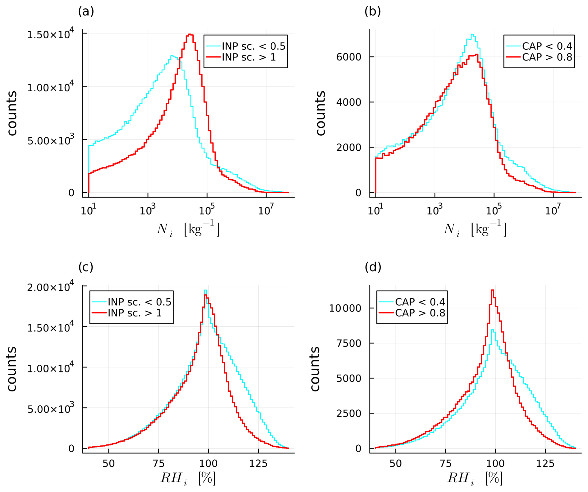
Figure 16 Histograms for N_i 5 h after the end of ascent, split according to the INP scaling factor in (a) and according to CAP in (b). The same for RH_i in (c) and (d). Only trajectories that do not descend after the end of the ascent are included.

For RH_i, CAP and the INP scaling factor are almost equally important (Table 3). They also have a very similar effect of increasing the tail of RH_i-values 5 h after the ascent to larger values while leaving the peak at ∼100 % unchanged (Fig. 16). For the INP scaling factor, this effect is a reflection of different N_i 5 h after the ascent (smaller N_i means slower reduction of supersaturation) and for CAP the signal simply occurs because larger CAP values reduce supersaturation faster.

6 Conclusions and Discussion

Warm-conveyor belts (WCBs) are a key feature for extra-tropical transport of humidity from the lower troposphere to the tropopause region. Due to the strong ascent and associated cloud formation this transport is modulated by cloud microphysical processes, the representation of which suffers from well-documented uncertainties in state-of-the-art weather and climate models. In this paper we therefore analyze Lagrangian trajectory data from a perturbed parameter ensemble (PPE) to answer the following research questions: (How) do perturbations in microphysical parameters and SST (i) influence thermodynamic and moisture conditions in fresh WCB outflow, (ii) alter hydrometeor distributions in fresh WCB outflow, (iii) impact the moisture and ice properties in aged WCB outflow, and (iv) how these effects vary with ascent velocity?

The distributions of T, p and q_v at the end of the ascent (research question (RQ) i) hardly vary across PPE members (Fig. 3a–f). This rigidity indicates that the thermodynamic conditions at the end of the ascent are constrained by the larger-scale environment and that parameter perturbations do not substantially influence their magnitude or distribution. In contrast, the RH_i distribution and its mean value varies quite strongly with INP scaling factor and CAP: When the INP scaling factor and CAP are small, the RH_i distribution has a sharp peak below 100 % and a long tail to larger values (Fig. 9a). If the INP scaling factor and CAP are large, the distribution is more Gaussian-shaped with a peak at about 102 %. We have shown that the differences in the RH_i distribution are caused by the impact of INP scaling factor and CAP on the ice crystal population, which is connected to RH_i by the timescale for super-saturation depletion τ_sat,ice (Eq. 2, Fig. 10).

The hydrometeor population at the end of ascent (RQ ii) is dominated by ice particles. The largest variation in ice mass and number mixing ratio are induced by the INP scaling factor and CAP: For a small CAP and INP scaling factor, the N_i distribution hints at bimodality with a second mode at large N_i values, that vanishes for larger CAP and INP scaling factors. This behavior can be explained by the more efficient cloud glaciation with large CAP values and INP scaling factor, which strongly reduces the number supercooled droplets reaching the homogeneous freezing level. For enhanced INP scaling factors we additionally detect a small shift for smaller N_i values, which correlates directly with the number of heterogeneously formed ice crystals. The ice crystal mass mixing ratio decreases with increasing CAP (and to a lesser extent with increasing INP scaling factor) due to the larger size of ice crystals and more efficient sedimentation.

Interestingly we find no significant impact of CCN scaling on the ice crystal population at the end of ascent, although it substantially modulates the hydrometeor population and onset of substantial glaciation during the ascent. However, this signature does not propagate to the fully glaciated state at the end of ascent. Also we do not find an impact of SST or SAT perturbations on the outflow ice crystal population. This absence of an effect is somewhat surprising, as Oertel et al. (2025) found altered fractions of fast ascending trajectories and Schwenk and Miltenberger (2024) showed that fast ascending trajectories contain more ice at end of ascent. However, the fraction of fast ascending trajectories is overall very small and therefore the impact on the overall distribution of q_i and N_i in the outflow are small.

Considering only fast-ascending trajectories (RQ iv), CAP and the INP scaling factor remain the most important parameters for hydrometeor content and RH_i at the end of the ascent (Figs. 12b and e, 13b), albeit with the a less pronounced impact on the RH_i distribution than for all trajectories. This small impact on RH_i is likely a consequence of the fast ascent and short timescale for glaciation, with some super-cooled liquid reaching the homogeneous freezing temperature irrespective of the choice of CAP and INP scaling factor. N_i and r_i are more sensitive to CAP and the INP scaling factor for fast ascending trajectories than for all trajectories.

This sensitivity indicates that simulation scale might also influence N_i and r_i, since Choudhary and Voigt (2022) found that a greater fraction of WCB trajectories ascend quickly when model resolution is increased. In contrast to the consideration of all trajectories, perturbations of the CCN scaling factor have small yet noticeable impact on q_i, N_i and RH_i distributions, with large CCN scaling factors shifting those distributions to smaller values. We also find a small impact of SAT perturbations on the thermodynamic conditions (p, T) and specific humidity q_v at the end of ascent (Fig. 14). The larger impact of SAT for fast-ascending trajectories is due to more substantial super-saturation being possible at larger vertical velocities and the larger fraction of the ascent spend in mixed-phase conditions, where water vapor-condensate partitioning is controlled by saturation adjustment. Therefore, altering SAT impacts buoyancy more strongly and enables a deeper ascent with an increasing SAT perturbation.

The ice particle population 5 h after the end of the ascent (RQ iii) is impacted mostly by the choice of CAP and the INP scaling factor. In comparison to end of ascent (RQ ii), the large N_i values (associated with small r_i) are not present anymore and crystals from the small N_i mode dominate. Consequently the INP scaling factor is more important than CAP 5 h after the end of ascent, while they were of similar importance at the end of ascent.

The analysis presented here is based on the PPE from Oertel et al. (2025), which focused on the dynamical impact of parameter perturbations, i.e. on the role for diabatically induced potential vorticity anomalies. Some earlier studies have also provided insight into the role of uncertainty in the microphysical parametrization for WCBs, but in contrast to our paper have predominantly focused on the impact on diabatically induced PV anomalies, upper-level flow and its predictability. In particular, Joos and Forbes (2016) investigated differences between two versions of the ECMWF global model (IFS) dominated by changes in the cloud microphysics scheme. Similarly, Mazoyer et al. (2021, 2023) explored the impact of using different cloud microphysics schemes available in the French Mesoscale Non-Hydrostatic model (MesoNH) in convection-permitting simulations. Pickl et al. (2022) investigated the effect of Stochastically Perturbed Parameterization Tendencies (SPPT) on WCBs using the IFS model at 100 km resolution, running simulations over multiple model years. In addition, recent studies have proposed a concept for objectively selecting impactful parameter perturbations (Hieronymus et al., 2022; Neuhauser et al., 2023). While their results partly align with the subjective parameter selection in our PPE, guidance from their results could be used to expand the investigation in future studies.

Our results suggest that in ICON's two-moment cloud microphysics scheme, the hydrometeor populations and RH_i-conditions in WCB outflow are sensitive to the parameter choices in the cloud microphysics scheme, specifically those relevant for microphysical processes in the ice phase (CAP and INP scaling factor). However, this study consists of only one case study using one microphysics scheme, and it isn't clear how representative our findings are of WCBs (or other model configurations and microphysics schemes) in general. Additionally, PPEs sample the uncertain multi-parameter phase space but assume constant parameter values throughout the simulation for some parameters that are not constant in reality. Therefore, sensitivities can be overestimated relative to a potentially more realistic stochastic framework in which parameters vary during the simulation (e.g Stanford et al., 2019). Furthermore, the microphysics scheme employed in the ICON simulation only considers rime splintering; it does not account for raindrop fragmentation upon freezing or ice collisional breakup for secondary ice production. This could result in biases in mixed-phase ice concentrations. Finally, there are likely additional important parameters that influence the variables examined in this study, but that were not perturbed (see Hieronymus et al., 2025). Nevertheless, the findings from this study lead to the following implications and practical recommendations for modeling, observation, and future research:

• The effects identified in this study could inform decisions for microphysical parameter choices in numerical models or parameters to be perturbed in ensemble prediction systems.

• Comparison of the distribution of N_i, q_i, r_i and RH_i documented here and distributions from large observational data-sets may help in selecting appropriate values for CAP and the INP scaling factor for WCB flow configurations.

• Future modeling studies on WCB moisture transport should keep CAP and the INP scaling factor, but reserve additional resources to investigate other potentially important factors such as the representation of graupel and ice sedimentation velocity or collision efficiencies of ice-phase particles.

• Our findings may have implications for geoengineering strategies such as cirrus cloud thinning (Lohmann and Gasparini, 2017), which aim to modify processes similar to those affected by the INP scaling factor. Since N_i 5 h after the ascend increases with the INP scaling factor 5 h after the ascent, accelerating these processes could pose a risk of “overseeding”, as discussed in Gasparini et al. (2020).

• Following this, future studies could investigate how the different UTLS moisture conditions produced by the PPE members influence the radiative effect of WCBs.

• The vertical water transport in WCBs is an important contribution to the water content and supersaturation distribution in the extra-tropical UTLS. Future studies should examine the impact of the changes found here for the occurrence of extra-tropical ice supersaturated regions, which impact downstream in-situ cirrus formation including aviation-induced cirrus.

Appendix A: Additional Figures

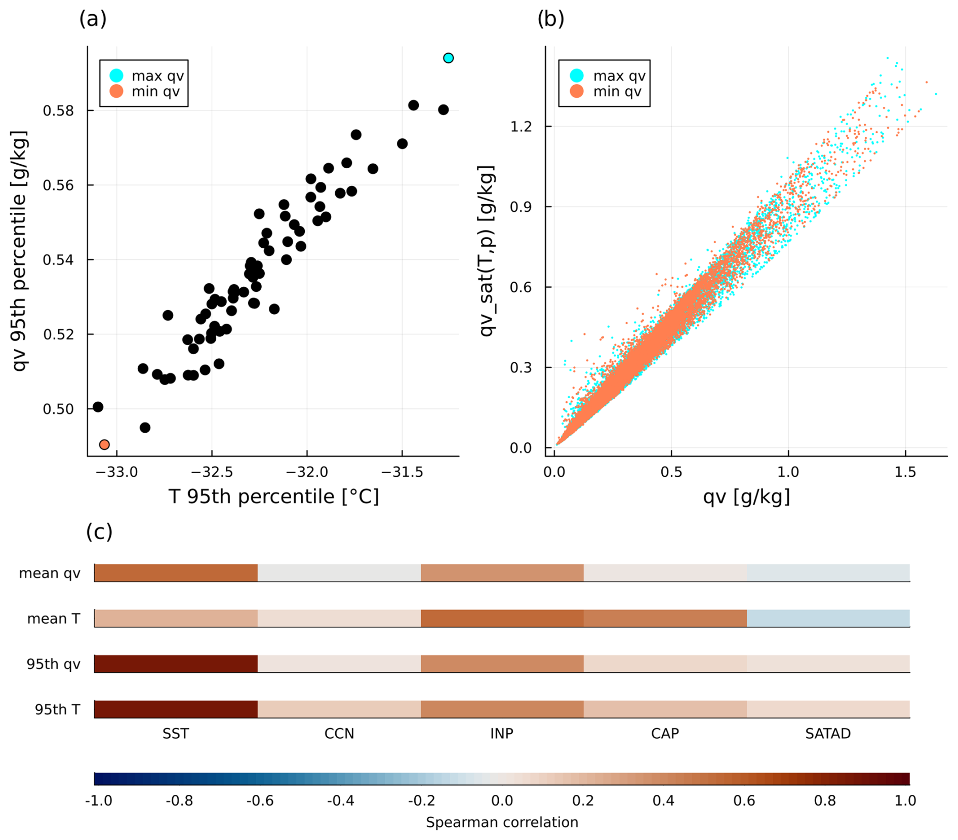
Figure A1 (a) Scatter-plot of 95th percentiles of q_v over T per ensemble member (dots). The ensemble members with the highest (lowest) 95th percentile of q_v values are plotted in cyan (orange). (b) Scatter-plot of saturation specific humidity (calculated using temperature and pressure of parcel) against specific humidity q_v for these two ensemble members. Panel (c) shows the Spearman correlation of mean and 95th percentile for q_v and T with all perturbed parameters.