Influence of secondary ice production on cloud and rain properties: analysis of the HYMEX IOP7a heavy-precipitation event

A significant part of precipitation originates from ice crystals; however, the representation of mixed-phase clouds by atmospheric models remains a challenging task. One well-known problem is the discrepancy between the concentration of ice-nucleating particles (INPs) and the ice crystal number concentration. This study explores the effect of secondary ice production (SIP) on the properties of the Intensive Observation Period 7a (IOP7a), an intense-precipitation event observed during the HYdrological Cycle in the Mediterranean EXperiment (HYMEX) campaign. The effect of SIP on cloud and rain properties is assessed by turning SIP mechanisms in the DEtailed SCAvenging and Microphysics (DESCAM) 3D bin microphysics scheme on or off. Our results indicate that including SIP gives better agreement with in situ aircraft observations in terms of ice crystal number concentration and supercooled drop number fraction. During the mature cloud stage and for temperatures warmer than −30 °C, 59 % of ice crystals are produced by fragmentation due to ice–ice collisions, 38 % by the Hallett–Mossop process, 2 % by fragmentation of freezing drops, and only 1 % by heterogeneous ice nucleation. Furthermore, our results show that the production of small ice crystals by SIP induces a redistribution of the condensed water mass toward particles smaller than 3 mm rather than toward larger ones. As ice crystals melt, this effect is also visible in the precipitating liquid phase. The shift toward smaller particles results in a reduced precipitation flux of both ice crystals and drops. Consequently, SIP induces a decrease in accumulated precipitation at the surface by 8 % and reduces heavy rainfall exceeding 40 mm by 20 %.

1 Introduction

The ice phase of clouds plays a crucial role in precipitation, contributing to $\mathrm{3}/\mathrm{4}$ of the Earth's surface precipitation (Heymsfield et al., 2020) by both snowfall and cold rain (i.e., melted ice particles). As shown by Gupta et al. (2023), the contribution of the ice phase to surface precipitation varies from 27 % for clouds with warm bases (e.g., tropical convective clouds) to up to 80 % for clouds with cold bases (i.e., close to the melting layer). Consequently, the role of ice crystals is particularly pronounced in mid- and high-latitude regions, where the majority of precipitation events are linked to ice crystals originating from mixed- or ice-phase clouds (Field and Heymsfield, 2015). Furthermore, incorporating the ice phase in models has been shown to significantly influence both the onset and the intensity of precipitation (Sawada and Iwasaki, 2007; Flossmann and Wobrock, 2010; Planche et al., 2014).

The properties and processes involving ice crystals are complex and remain poorly understood. Indeed, unlike water drops, ice crystals exhibit a wide variety of shapes influenced by processes such as vapor deposition, riming, and aggregation. In addition, major uncertainty still persists regarding the mechanisms driving their formation. Although heterogeneous ice nucleation, which is the first pathway for ice crystal formation at T > −30 °C, has been intensely studied (e.g., Kanji et al., 2017), this process is highly variable as it depends on the physico-chemical properties of aerosol particles. Furthermore, it has long been recognized that heterogeneous ice nucleation alone is often insufficient to explain the observed concentrations of ice crystals in clouds, as shown by in situ aircraft observations of Hallett et al. (1978), Hobbs et al. (1980), and Mossop (1985) or more recently by Ladino et al. (2017), Järvinen et al. (2022), and Korolev et al. (2022). This indicates the presence of secondary ice production (SIP), which generates additional ice crystals from existing ones. Some of the SIP mechanisms presented by Field et al. (2017) or Korolev and Leisner (2020) have recently been incorporated into numerical models. Modeling studies have highlighted several important effects induced by SIP, such as its impact on convection (Dedekind et al., 2021; Karalis et al., 2022; Qu et al., 2022; Grzegorczyk et al., 2025b), precipitation (Hoarau et al., 2018; Dedekind et al., 2021; Georgakaki et al., 2022; Lachapelle et al., 2024), and radiative properties (Young et al., 2019; Zhao and Liu, 2021; Waman et al., 2023). However, the mechanisms driving SIP and the understanding of its effects on cloud properties remain open research questions.

Two previous studies (i.e., Kagkara et al., 2020; Arteaga et al., 2020), conducted with the DEtailed SCAvenging and Microphysics (DESCAM; Flossmann and Wobrock, 2010) 3D bin microphysics scheme, focused on an intense-precipitation event (IOP7a) observed during the HYdrological Cycle in the Mediterranean EXperiment (HYMEX) campaign (Ducrocq et al., 2014). The HYMEX campaign (Ducrocq et al., 2014) aims to study flash flood events that often occur in the western Mediterranean Basin (e.g., Sénési et al., 1996; Delrieu et al., 2005; Rebora et al., 2013) by means of different observational facilities. The cloud systems responsible for these events are driven by warm and humid air masses originating from the Mediterranean Sea, which are lifted over the French coastal mountainous terrain. One of the main conclusions found in Kagkara et al. (2020) was the lack of ice particles smaller than 1 mm in diameter given by DESCAM close to the −12 °C level, while SIP was not included in the model at that time.

Therefore, the Hallett–Mossop process (also known as splintering during riming) (Hallett and Mossop, 1974), fragmentation due to ice–ice collisions (Grzegorczyk et al., 2023; Yadav et al., 2024), and drop shattering (fragmentation of freezing drops) (Lauber et al., 2018; Keinert et al., 2020) are SIP processes that have recently been implemented in DESCAM by Grzegorczyk et al. (2025a). These processes were tested using an idealized scenario of a deep tropical convective cloud, as encountered during the High Altitude Ice Crystals and High Ice Water Content (HAIC/HIWC) campaign in French Guyana (Fontaine et al., 2020; Hu et al., 2021). The results of Grzegorczyk et al. (2025a) for these tropical conditions showed that incorporating SIP processes reduces supercooled liquid water, while ice water content and ice crystal number concentration increase, improving agreement between model outcomes and in situ aircraft observations. Furthermore, using the same idealized tropical convective case, Grzegorczyk et al. (2025b) showed that SIP affects both convection and precipitation properties, reducing the cloud top height by about 1.5 km and the total precipitation accumulation by 15 %. However, these results need to be confirmed under real cloud conditions among different cloud types, and the causes of the observed reduction in precipitation require further investigation.

Building on our previous findings, this study aims to investigate the impact of SIP on the mixed phase of a mid-latitude precipitating convective cloud (i.e., the HYMEX IOP7a heavy-precipitation event) and validate the DESCAM model results through comparisons with in situ aircraft measurements. Additionally, since a significant portion of precipitation may originate from ice, the second goal of this study is to assess and understand the impact of SIP on precipitation properties simulated by DESCAM, which is confronted against ground-based observations.

The paper is organized as follow. Section 2 provides a general description of the IOP7a event and an overview of the observations available for this case. Section 3 details the numerical setup of the study and the methodology used to compare the model results to the observations. Results focusing on the cloud mixed-phase properties are presented in Sect. 4.1, while liquid rain properties are presented in Sect. 4.2. Finally, Sect. 5 summarizes the study and highlights the main conclusions.

2 Observations

2.1 HYMEX IOP7a case

The HYMEX program was a 10-year research project dedicated to studying the Mediterranean water cycle (Drobinski et al., 2014). This program included a long-term observation period spanning 2010 to 2020 and two special observation periods (SOPs). The present case study took place during SOP1 in autumn 2012 (Ducrocq et al., 2014), focusing on flash flooding events in the northern Mediterranean Basin. During this experimental period, a variety of observational facilities, such as radars, rain gauges, disdrometers, radiosondes, and research aircraft, as well as several other instruments, were deployed in addition to the existing observation networks in the Cévennes–Vivarais region in France.

This study focuses on the seventh Intense Observation Period (IOP7a), which took place in the morning of 29 September 2012, (already studied by Hally et al., 2014; Kagkara et al., 2020; Arteaga et al., 2020). This event was characterized by the presence of a low-pressure system near the United Kingdom and a cold front west of the Cévennes–Vivarais region. These conditions generated a southerly wind flow transporting warm and moist air from the Mediterranean Sea toward the Cévennes mountains. The orographic lifting of this air mass triggered the formation of mesoscale convective systems over the mountainous region. More details about the development of such cloud systems can be found in Duffourg and Ducrocq (2011) and Nuissier et al. (2011).

2.2 Ground and airborne observations

During IOP7a, the Application Radar à la Météorologie Infra-Synoptique (ARAMIS) operational network, comprising C-, S-, and X-band radars covering the Cévennes–Vivarais region (Parent du châtelet, 2003), along with three rain gauge networks (from Météo France, Tardieu and Leroy, 2003; Service de Prévision des Crues (SPC) du Grand Delta; and Electricité de France (EDF)), allow for the derivation of quantitative precipitation estimates. These estimates are obtained by using the kriging with external drift (KED) method developed by Boudevillain et al. (2016) and Delrieu et al. (2014). This approach consists of merging radar data with rain gauge measurements to produce hourly estimates of the precipitation fields over the Cévennes–Vivarais region.

Moreover, two Parsivel disdrometers (OTT Parsivel²) were deployed at La Souche and Saint-Étienne de Fontbellon (StEF), as shown in Fig. 1. These instruments provide 1 min resolution rain rates and raindrop size distributions (DSDs) using the method of Raupach and Berne (2015). The disdrometer at StEF, located at an altitude of 302 m, recorded the precipitation event from 08:20 to 08:50 UTC and showed a maximum intensity of around 100 mm h⁻¹. The second disdrometer at La Souche, located at 920 m, recorded the precipitation event from 09:40 to 11:00 with a maximum rain rate of 175 mm h⁻¹. A detailed study of DSDs from these instruments is presented by Zwiebel et al. (2015).

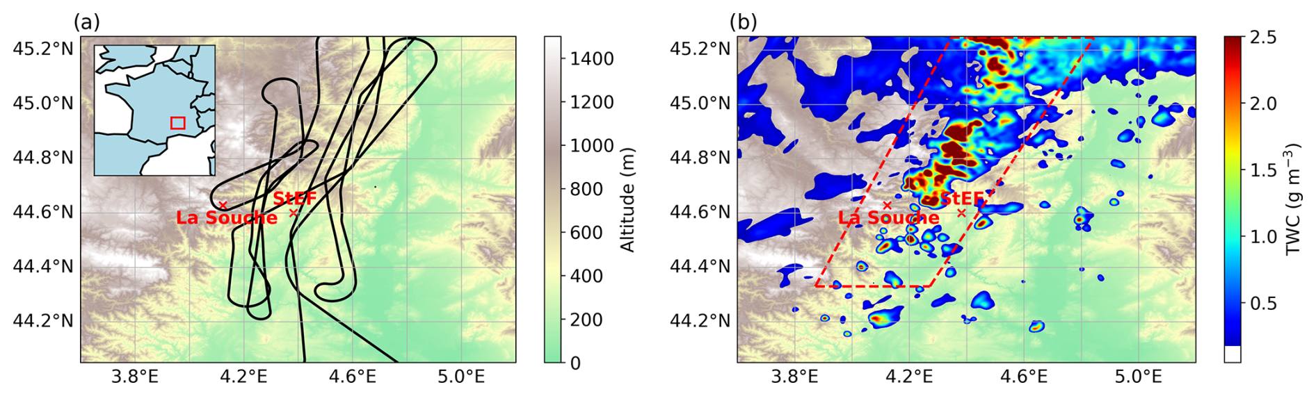
Figure 1 Third domain of the simulation, with the topography and the Falcon 20 flight track in panel (a). Total water content at 08:20 UTC and 4.7 km (SIP simulation) is displayed in panel (b). The dashed red lines delimit the area of the domain selected for comparison with in situ observations. The positions of the La Souche and Saint-Étienne de Fontbellon (StEF) disdrometers are indicated by red crosses.

In addition to ground-based observations, two French research aircraft operated by Service des Avions Français Instrumentés pour la Recherche en Environnement (SAFIRE) were deployed during HYMEX IOP7a. The first aircraft (ATR-42) flew around 100 to 150 km south of the precipitation event and was dedicated to studying aerosol particles (see Rose et al., 2015, for details) that were advected to the Cévennes–Vivarais region and contributed to the formation of the cloud system. This aircraft was equipped with a scanning mobility particle sizer (SMPS) instrument and a GRIMM optical particle counter (OPC). From these two instruments, aerosol particle size distributions for diameters ranging from 20 nm to 2 µm were obtained for altitudes between 200 and 3700 m. The second aircraft (Falcon 20), dedicated to cloud microphysics measurements, was equipped with a W-band Doppler radar (RASTA) and two optical array probes (OAPs): a 2D-stereo (2DS) probe and a precipitation imaging probe (PIP). These two probes provided composite hydrometeor particle size distributions from 50 µm to 6.4 mm in diameter. For smaller sizes, a cloud droplet probe (CDP) instrument provided particle size distributions from 2 to 50 µm in diameter.

Figure 2 presents the temporal evolution of microphysics measurements conducted by Falcon 20 during IOP7a. In Fig. 2a both radar reflectivity (in dBZ) and aircraft altitude above sea level are shown. The cloud system was sampled at different constant heights: at 3.7 km, twice near 5.5 km, at 7 km, twice at 8.5 km, and at 10.5 km. Complementary to this, Fig. 1a shows the flight track of the Falcon 20 aircraft, which flew close to the two disdrometer sites deployed during IOP7a.

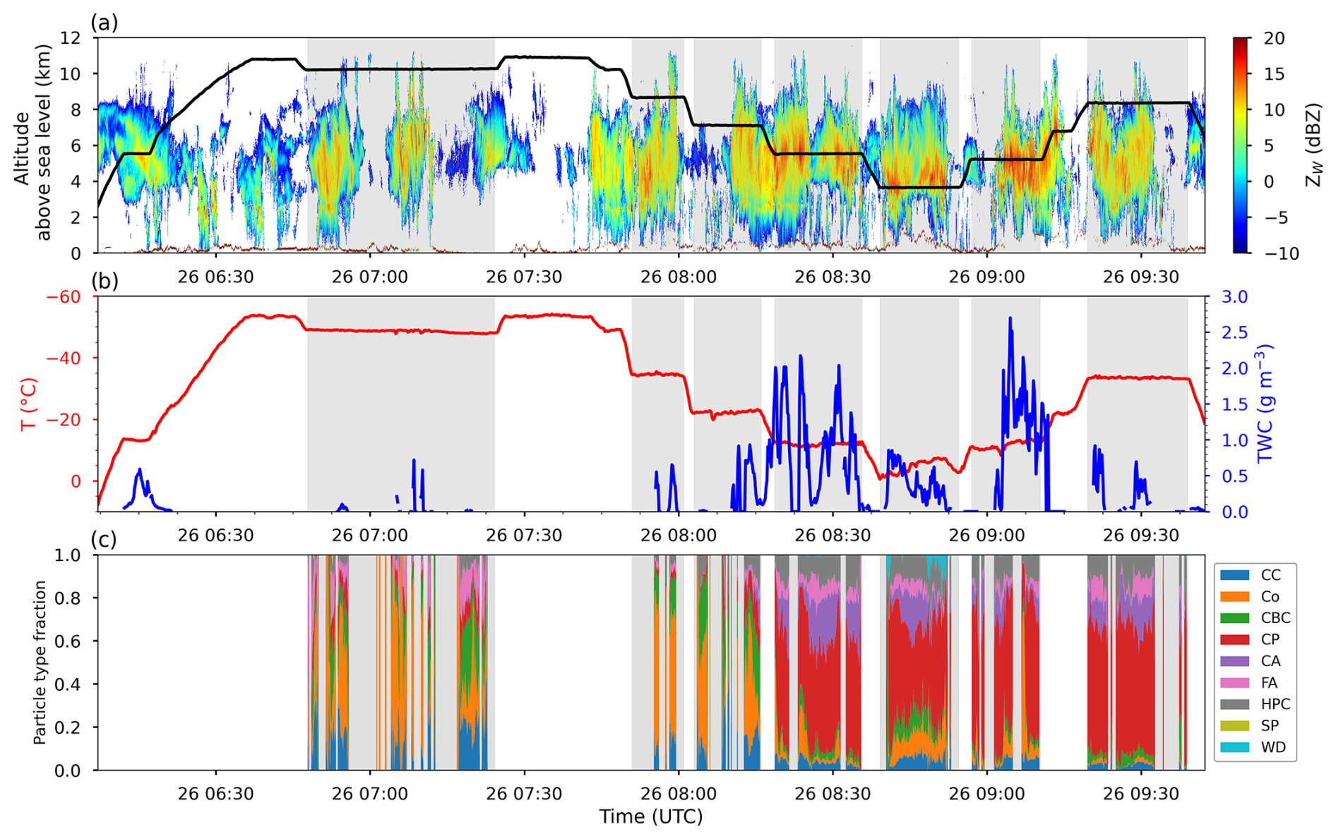
Figure 2 Time–height measurements conducted by Falcon 20 during IOP7a. (a) RASTA W-band radar reflectivity observation and aircraft altitude (reflectivity values within ±300 m of the aircraft are interpolated). (b) Temperature and total water content (TWC) estimated using the method of Fontaine et al. (2014). (c) Time series (10 s averaged) showing the fraction of hydrometeor types with D > 300 µm classified as capped columns (CC); columns and needles (Co); a combination of bullets and columns (CBC); compact particles (CP); complex assemblages of planes, columns, or dendrites (CA); fragile aggregates (FA); hexagonal planar crystals (HPC); splintered particles (SP); and water drops (WD), following the method developed by Jaffeux et al. (2022).

Figure 2b shows the air temperature and the estimated total water content (TWC). The TWC is determined by the following equation: TWC = ${\sum }_{\mathrm{50}\mathrm{\mu }\mathrm{m}}^{\mathrm{6400}\mathrm{\mu }\mathrm{m}}N\left(D\right)\mathit{\alpha }{D}^{\mathit{\beta }}\mathrm{d}D$, where N(D) is the number of particles with diameter D, and the coefficients α and β are the coefficients of the mass size relationship (m(D) = αD^β) determined by the variational method proposed by Fontaine et al. (2014). In this method, α is determined by fitting the simulated radar reflectivity (T-matrix method) with measurements from the RASTA radar on board the aircraft. β is derived from the surface–diameter relationship based on ice crystal images captured by the OAPs. Note that, in contrast to the model, the estimated TWC is estimated from particles smaller than 6.4 mm. In the context of another airborne campaign, where an isokinetic total water content evaporator (IKP-2; Strapp et al., 2016) probe was deployed, Fontaine et al. (2017) showed that the method used here to estimate the TWC overestimates it by about +16 % compared to direct measurements of TWC with the IKP-2 probe.

Figure 2c presents the time series of the fraction of hydrometeor types. The classification of these hydrometeors is carried out by the algorithm developed by Jaffeux et al. (2022), which employs a convolutional neural network (CNN) to process non-truncated particle images larger than 300 µm, recorded by the 2DS probe. Particles are assigned to a specific hydrometeor type if the algorithm gives a probability of attribution exceeding 50 % for that type.

Based on over 1 million particle images processed, Fig. 2c shows that columnar ice crystals (COs) are prevalent in areas with low radar reflectivities before 08:15 UTC. After that time, compact particles (CPs) dominate, radar reflectivity increases (see Fig. 2a), and strong updrafts are measured (not shown here), which is characteristic of a convective region. Additionally, these areas exhibit the highest TWC values, suggesting that the riming process is particularly efficient in forming ice, which aligns with the occurrence of CPs. It is also important to note that the fraction of water drops (WDs) is almost negligible throughout the flight, with the exception of a localized peak reaching up to 20 % near the melting layer (at 3.7 km).

3 Model setup

3.1 Numerical experiment

Simulations of this study are performed using the DESCAM bin microphysics scheme (Flossmann and Wobrock, 2010) implemented in the 3D dynamical model of Clark et al. (1996) and Clark (2003). DESCAM encompasses size distributions for the number of aerosol particles, cloud droplets, and ice particles, with 39 bins each. Two further size distributions give the aerosol mass inside each droplet and each ice crystal bin. Another distribution function describes rime mass included in each ice particle and is restricted to 27 bins (i.e., > 32 µm ice particles). The evolution of all 222 bins is determined by individual budget equations respecting transport processes (advection, turbulence, and sedimentation) and source and sink terms given by cloud microphysics. The microphysics processes included in DESCAM are drop nucleation; deactivation; condensation; collision–coalescence; and heterogeneous and homogeneous ice nucleation, ice deactivation, vapor deposition growth, riming, and aggregation. Three SIP processes were recently implemented in DESCAM (see Grzegorczyk et al., 2025a, b). Although the SIP parameterizations and implementation in DESCAM are detailed in Grzegorczyk et al. (2025a), a brief summary is given hereafter, and more details are available in Appendix A.

The first SIP process considered in DESCAM is the Hallett–Mossop (HM) process, which is activated between −3 and −8 °C. It is temperature dependent within this temperature range, reaching a maximum of 350 fragments per milligram of rime produced at −5 °C (Hallett and Mossop, 1974). This temperature dependency is based on Eq. (72) of Cotton et al. (1986). More details about HM are presented in Sect. A1 of Appendix A.

The second process implemented in DESCAM is drop shattering during freezing (DS), parameterized following Phillips et al. (2018). It includes two modes: mode 1, which occurs during collisions between droplets with smaller ice crystals or through heterogeneous freezing, and mode 2, which occurs when raindrops are accreted by more massive ice particles. The equations taken from Phillips et al. (2018) used in DESCAM are presented in Sect. A2 of Appendix A.

Finally, fragmentation due to ice–ice collisions (BRK) is based on the formulation by Phillips et al. (2017a) but with parameters derived from the laboratory study of Grzegorczyk et al. (2023) for graupel and snow aggregate fragmentation experiments. Since DESCAM does not categorize ice particles but predicts their rime mass, the breakup of ice particles with less than 50 % rime mass follows snow aggregate behavior, while those above 50 % follow graupel behavior. A full description of the BRK parameterization in DESCAM is given in Sect. A3 of Appendix A.

In DESCAM, SIP is also determined by the collision rates of hydrometeors, which requires solving the stochastic collision equations for ice–droplet collisions (for HM and DS) and ice–ice collisions (for BRK), following the method of Bott (1998).

To assess the effects of SIP processes on both the liquid and the ice phases, two simulations are run, one with the three SIP processes activated (called “SIP” simulation) and the other without any SIP processes (called “no-SIP” simulation). The numerical setup is identical to the one used in Kagkara et al. (2020). It consists of three nested domains with horizontal resolutions of 8, 2, and 0.5 km. The vertical resolution of the three domains is non-equidistant with Δz = 40 m near the ground and increasing continuously to Δz = 230 m at 9 km. The third domain is centered over the Cévennes–Vivarais region, where ground and in situ measurements were conducted, as shown in Fig. 1. The simulations are performed from 00:00 to 12:00 UTC on 25 September 2012 (IOP7a case), with a time step Δt = 2 s. The initiation and boundary conditions are forced from IFS ECMWF data at 6 h intervals. Aerosol particle concentration and size distribution used for the model initiation are derived from measurements conducted by the ATR-42 aircraft, which flew 150 km further south of the cloud system. These measurements showed a concentration of 3000 cm⁻³ aerosol particles near the ground, which corresponds to a polluted situation. This is consistent with the continental origin of the air masses coming from Spain (see Kagkara et al., 2020, for further details).

3.2 Comparison with observations

Figure 1a displays the flight track over the third domain of the model, while Fig. 1b shows the model area (indicated by the dashed red lines) selected for the comparisons with the in situ observations. Considering the selected area in Fig. 1b ensures that the cloud system is compared with aircraft observations from a corresponding region shown in Fig. 1a. Furthermore, the simulated ice water content (IWC) at 4.7 km altitude for 08:20 UTC is also shown in Fig. 2b. Airborne in situ observations at the same time, illustrated in Fig. 1b, confirm the presence of high TWC.

To compare simulation results to the in situ observations, only measurements taken at constant altitudes (indicated by the shaded areas in Fig. 2) were taken into account. Additionally, we only considered model grid points within the area shown by dashed lines in Fig. 1b, where TWC and vertical wind speeds ranged from 0.01 to 2 g m⁻³ and −4 to +3 m s⁻¹, respectively, corresponding to the 5th–95th percentile range of the airborne measurements. In contrast to selecting grid points near the aircraft track, this method ensures that the model closely matches the observed conditions, excluding strong convective regions where no measurements were made for safety reasons. It also allows the selection of much more data points in the model, leading to a better statistical significance and improving the robustness of the comparison.

The model results at 08:20 UTC are selected for comparison with the observations, as this time is right in the middle of the 2 h period of in situ measurements. During this interval, the simulated cloud was developed at its mature stage and stationary over the mountainous regions. Consequently, model results show only small variations during the time span from 07:30 to 09:30 UTC and thus lead to the same conclusions.

4 Results

4.1 Mixed-phase properties

To evaluate whether DESCAM can reproduce the properties of the observed cloud system, Fig. 3a shows the average total water content (TWC) profiles of the SIP and no-SIP simulations compared with the mean observed TWC estimated from in situ measurements.

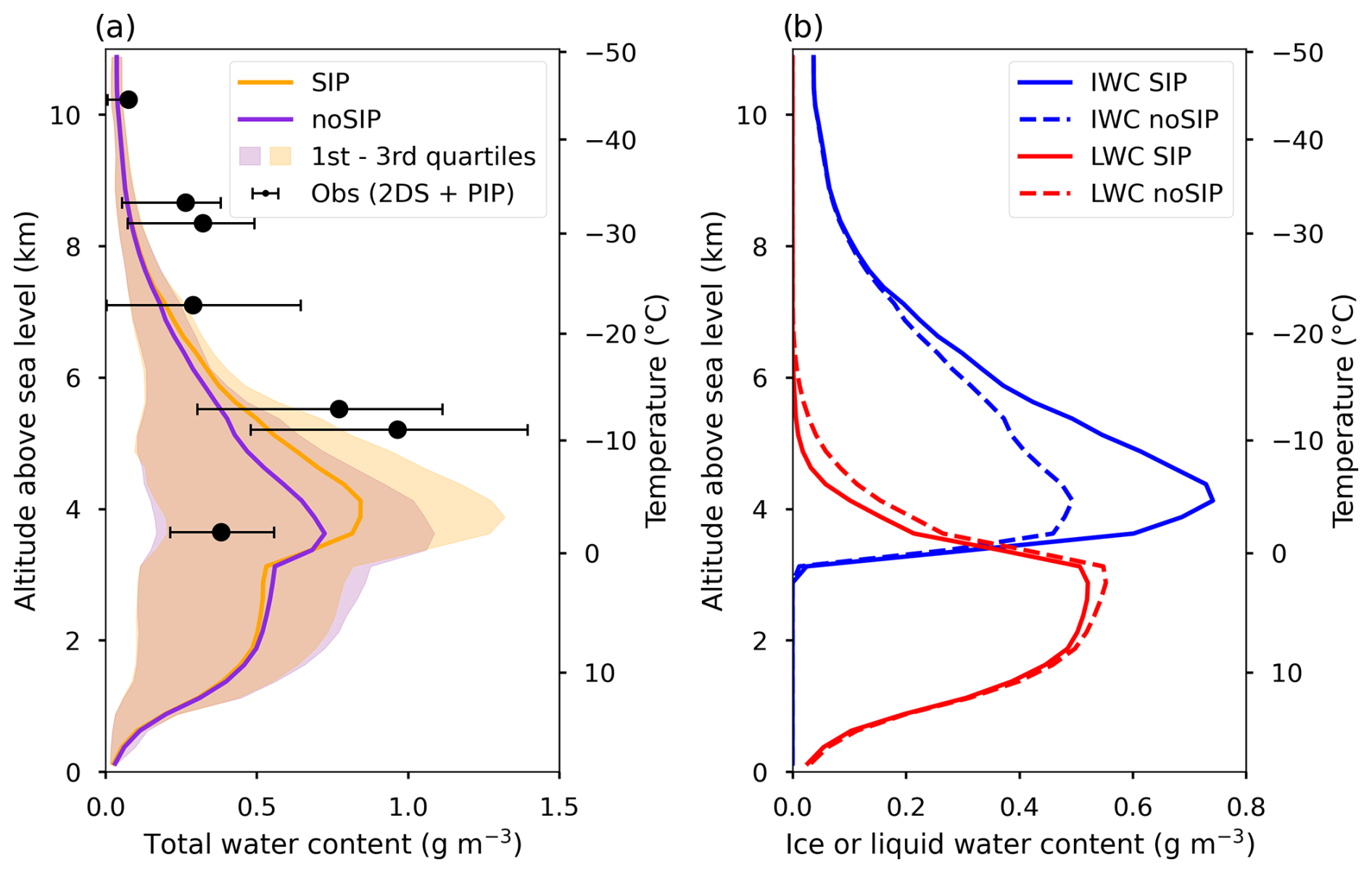
Figure 3 (a) Vertical mean profiles of total water content (TWC) for SIP and no-SIP simulations, as well as observed TWC. The error bars and shaded area show the first and third quartiles of observations and both simulations, respectively. (b) Vertical mean profiles of ice water content (IWC) and liquid water content (LWC) for SIP and no-SIP simulations. (Note that the x axis is different.)

While the simulated TWC profiles follow a similar trend compared to the observed TWC, the amount of TWC for SIP and no SIP underestimates the values observed in some flight levels by about 50 %. However, it is important to note that the observed TWC is based on indirect measurements, which probably overestimate the TWC slightly (16 % according to Fontaine et al., 2017), and should therefore be interpreted with caution. Nevertheless, both simulations are within the variability range of the observed TWC.

Figure 3a also shows that the SIP case has a higher TWC in the mixed-phase region (0 to −25 °C) and slightly lower TWC in the liquid phase (T > 0 °C) compared to the no-SIP case. These differences can be explained by the ice water content (IWC) and liquid water content (LWC) profiles (Fig. 3b). Indeed, within the mixed-phase regions, the SIP simulation gives higher IWC values, reaching a maximum of 0.74 g m⁻³ at 4 km altitude compared to 0.49 g m⁻³ in the no-SIP simulation at the same height. In contrast, in both the liquid and the mixed-phase regions, the LWC decreases by up to 0.05 g m⁻³ in SIP simulation. These differences arise from the increased number of ice crystals in the SIP simulation (see Fig. 4), which enhances vapor deposition, riming, and drop evaporation, as reported by Dedekind et al. (2021) or Grzegorczyk et al. (2025b). This specific result is further discussed in the following paragraphs.

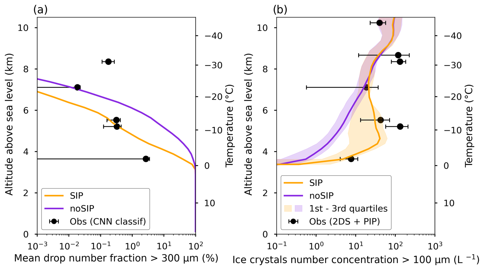
Figure 4 (a) Vertical mean profiles of the drop number fraction (> 300 µm) from the SIP and no-SIP simulations at 08:20 UTC compared with the fraction derived from the CNN classification. (b) Vertical mean profiles of ice crystal number concentration (N_ice) for particles larger than 100 µm from both simulations and the 2DS probe and PIP measurements. Error bars and shaded areas indicate the first and third quartiles.

Figure 4a presents the mean number fraction of water drops larger than 300 µm from in situ observations and from no-SIP and SIP simulations. The observed fraction is obtained from the ratio of the particle number classified as water drops by the CNN algorithm to the total number of other particle types (Jaffeux et al., 2022). In Fig. 4a, the mean fraction of drops is lower than 10 %, which is consistent with Fig. 2c, where the time series of water drop (WD) particles never exceeds 20 % of the total particle number.

Figure 4a shows that the SIP simulation gives a drop fraction that is 1 order of magnitude lower than the no-SIP simulation across all altitudes. Consequently, for temperatures warmer than −20 °C, the SIP simulation is closer to the observed drop fraction, particularly near −10 °C. However, around 0 °C, the drop fraction in the SIP simulation remains too high. This could be explained by the fact that melting is set to occur instantaneously (in contrast to Planche et al., 2014), which could lead to an overestimation of the supercooled drop number (with D > 300 µm) near 0 °C. For T < −20 °C, it is important to note that in two cases (at 8.5 and 10 km), the observed drop fraction is zero, and these points are therefore not represented in Fig. 4a. Three of the four drop fraction points observed at T < −20 °C (two zeros and a 0.02 % value at 7.5 km) presented in Fig. 4a correspond to stratiform conditions (i.e., before 08:15 UTC), while the fourth and highest drop fraction (0.2 % at 9 km) corresponds to convective conditions (after 08:15 UTC). This highlights that the drop fraction at these altitudes is highly dependent on the environmental conditions. However, with only four data points that vary significantly, it remains difficult to determine which simulation better matches the observations near the cloud top. Additional observations are needed to better evaluate the liquid and ice partitioning in DESCAM depending on environmental factors such as the convective and stratiform cloud regions observed before and after 08:15 UTC. Furthermore, even if the same size ranges of hydrometeors are compared, the present analysis should still be interpreted with caution, as the observed drop fraction is based on a CNN classification algorithm for 2DS probe images sampled by the aircraft in a limited portion of the cloud system.

The mean observed and simulated ice crystal number concentration (N_ice) for ice crystals over 100 µm is presented in Fig. 4b. Since the mean observed drop fraction for > 300 µm particles presented in Fig. 4a reaches only a maximum of 3 % next to the melting layer (3.5 km) and the modeled drop fraction for > 100 µm particles at this level (not shown here) is only about 1 order of magnitude higher than that for particles > 300 µm, we regard all particles larger than 100 µm detected by the 2DS probe and PIP as ice crystals. Therefore, we consider these measurements to be comparable to N_ice (> 300 µm) in DESCAM. This hypothesis is also commonly used when comparing model results to in situ aircraft measurements with, for example, > 75 µm particles in Arteaga et al. (2024) or even > 50 µm particles in Grzegorczyk et al. (2025a). This assumption can be further confirmed when looking at the combined 2DS probe and PIP measurements and the CDP measurements presented in Fig. 6, depicting the rise of particle numbers from 100 µm up to 300 µm, which probably corresponds to the deposition growth mode of ice particles.

As expected, N_ice in the SIP simulation significantly increases for T > −20 °C, reaching a maximum of 50 L⁻¹ at −5 °C. Furthermore, N_ice rises at 10 L⁻¹ near 0 °C in the SIP simulation, which is close to the observations, compared to only 0.5 L⁻¹ in the no-SIP simulation. At −12 °C, the SIP simulation gives 40 L⁻¹, which is significantly higher than 5 L⁻¹ in the no-SIP simulation. However, at this temperature level, the observations report even higher values of 50 and 100 L⁻¹. At temperatures colder than −20 °C, the N_ice profiles from no SIP and SIP are nearly identical, matching with observations at the −20 and −45 °C levels.

To further explain the variability of N_ice presented by Fig. 4b, Fig. 5 shows the mean vertical profiles of ice crystal production in the SIP simulation. In Fig. 5, the Hallett–Mossop (HM) process is the most efficient process, with its maximum (around 3 × 10⁻⁴ cm⁻³ s⁻¹) occurring at −5 °C, where N_ice and IWC reach their maximum (see Figs. 4b and 3b). Even though the maximum production rate of fragmentation due to ice–ice collisions (BRK) is about 3 times lower than HM, BRK remains efficient from 3.5 to 8 km with up to 10⁻⁴ cm⁻³ s⁻¹. Regarding the process of drop shattering during freezing (DS), mode 2 is efficient close to the melting layer when T > −5 °C conjointly with BRK, while mode 1 is 2 orders of magnitude lower than BRK and HM below −5 °C. The limited efficiency of DS is consistent with the low drop number fraction (D > 300 µm) presented in Fig. 4a, indicating an insufficient number of raindrops to make DS as effective as HM or BRK. While the rate of heterogeneous ice nucleation is around 10⁻⁷ cm⁻³ s⁻¹ at temperatures warmer than −10 °C (not represented in Fig. 5), this process becomes dominant at temperatures colder than −20 °C, when SIP processes are less efficient. It is also important to note that homogeneous ice nucleation is especially effective next to the cloud top.

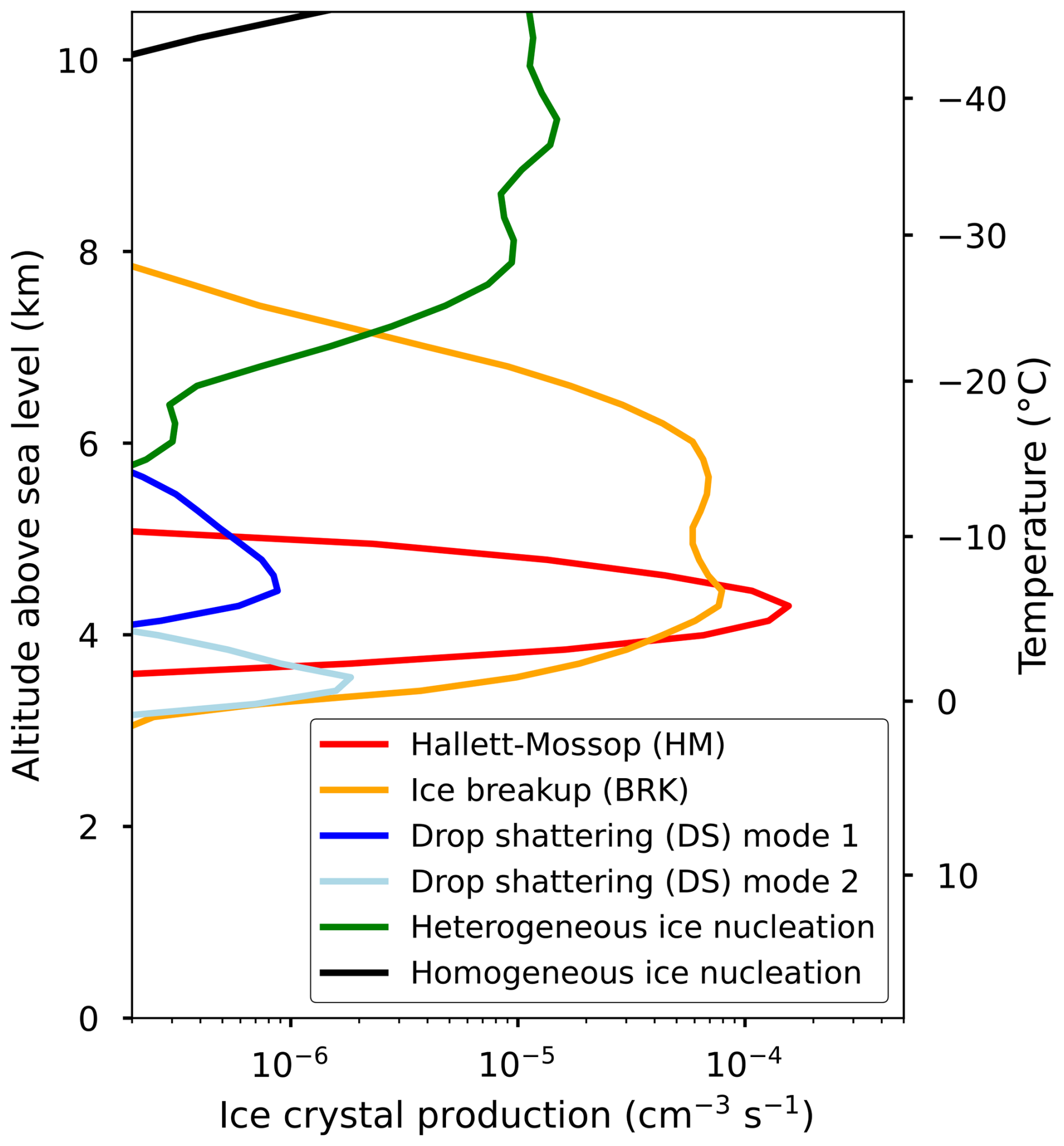
Figure 5 Vertical profiles of average ice crystal production rates from secondary and primary ice processes at 08:20 UTC for IWC = (0.01,2) g m⁻³ within the selected area inside the third domain (see Fig. 1b).

The results depicted by Fig. 5 show that HM and BRK are the most productive processes, which is consistent with the conclusions of Grzegorczyk et al. (2025b) for the tropical deep convective cloud case simulated by DESCAM. However, in the present case, the HM process plays a more significant role, producing 38 % of ice particles (compared to 17 % in Grzegorczyk et al., 2025b), while BRK accounts for 59 % (compared to 81 % in Grzegorczyk et al., 2025b). Furthermore, all production rates for this case are 1 order of magnitude lower than in the deep convective cloud case of Grzegorczyk et al. (2025b). As the IOP7a cloud case is less convective, it results in smaller IWC, which may inhibit SIP and the BRK process, which depends on the number and mass of colliding ice particles. For the other processes, similarly to Grzegorczyk et al. (2025b), we found that DS produced only 2 % of ice crystals, and heterogeneous ice nucleation accounted for 1 % for T > −30 °C.

To highlight the features of ice and liquid cloud phases, Fig. 6 shows the modeled mean particle size distributions (PSDs) of ice crystals and drops for SIP and no-SIP simulations at altitudes of 5 to 6 and 7 to 7.5 km, corresponding to three steady flight altitudes in Fig. 2. These modeling results are compared with the composite PSD (merged observations of PIP and 2DS probe) and the size distribution for droplets smaller than 50 µm from the CDP, observed at similar altitudes (i.e., 5.2, 5.5, and 7.1 km).

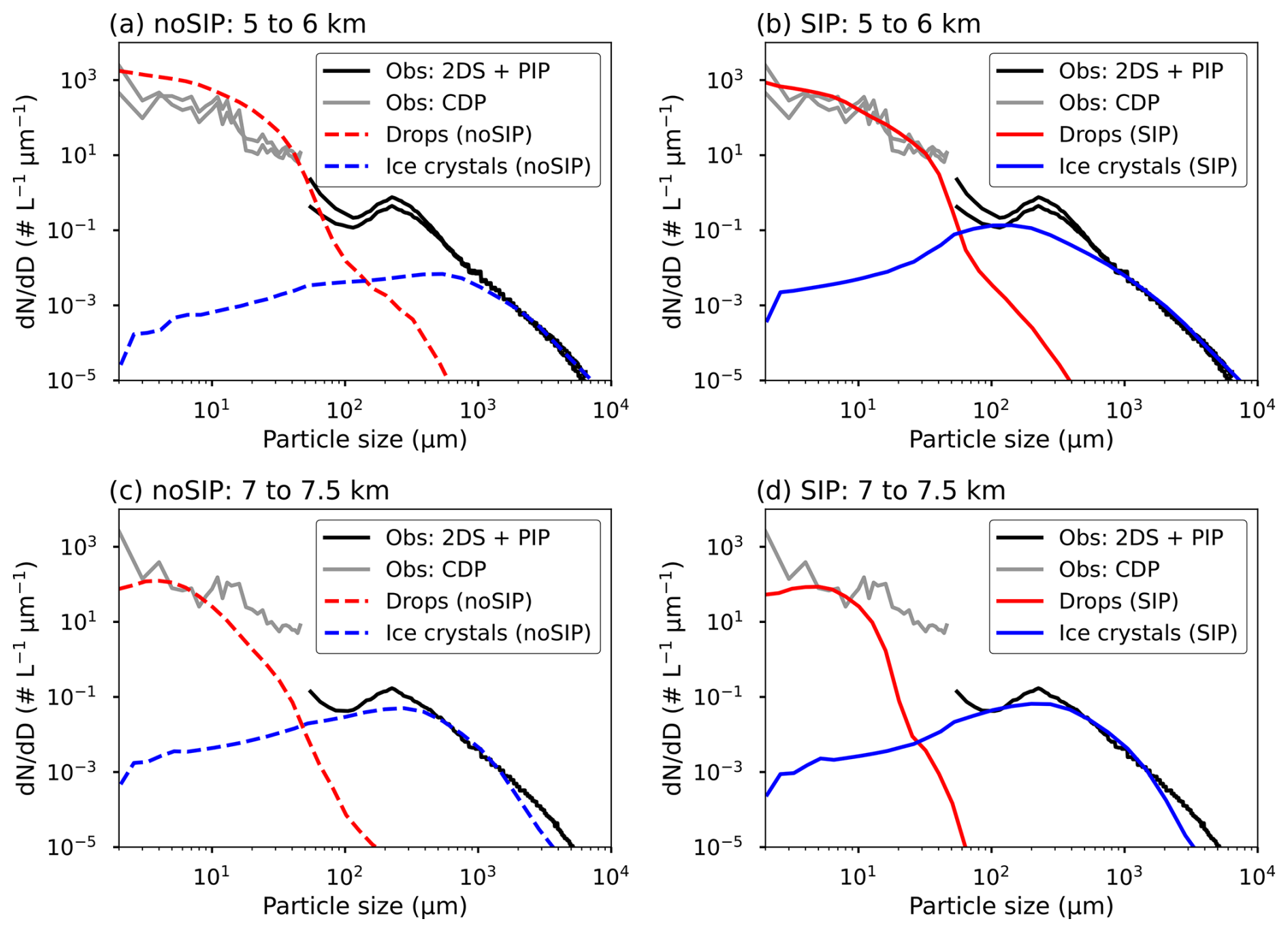
Figure 6 Mean drop and ice crystal particle size distributions (PSDs) of no-SIP and SIP simulations from 5 to 6 km in panels (a) and (b) compared with the mean measured PSDs of the merged 2DS probe and PIP (for D > 50 µm) and CDP (for D < 50 µm) at 5.2 and 5.5 km. The same results are presented for both simulations from 7 to 7.5 km in panels (c) and (d) and are compared with observations at 7.1 km.

In Fig. 6a, at 5.5 km (−12 °C), the no-SIP simulation underestimates the number concentration of ice crystals smaller than 2 mm compared to the observations (2DS and PIP), as assessed in Kagkara et al. (2020). Consequently, the mode of the ice crystal PSD is close to 700 µm for this simulation, while it is observed at 200 µm by the measurements. Additionally, the no-SIP simulation overestimates the droplet concentration by approximately 3 times compared to the CDP measurements. The SIP simulation (Fig. 6b) provides a higher concentration of small ice crystals, up to 30 times more than the no-SIP simulation close to 100 µm, which better matches the observed PSD at 5.5 km. However, the concentration of ice crystals near 200 µm still appears to be underestimated by a factor of 3. Furthermore, in the SIP simulation, the concentration of droplets smaller than 50 µm is lower and thus in better accordance with the CDP measurements, which indicate around 4500 L⁻¹.

Figure 6c and d also show drop and ice particle size distributions for the no-SIP and SIP simulations but for altitudes between 7 and 7.5 km (i.e., around −22 °C). For this level, the results from SIP and no-SIP simulations do not differ significantly, consistent with the fact that heterogeneous ice nucleation becomes more dominant than SIP processes below −20 °C (see Fig. 5). This shows that the cloud properties were already well represented without any SIP processes at this level. However, including SIP leads to a significant decrease in the number of droplets with D > 10 µm, probably due to their consumption at lower levels by riming or depositional growth of ice crystals generated by SIP. Consequently, this reduces agreement with the CDP measurement. This result is also consistent with the lower drop fraction given in the SIP simulation for this level (see Fig. 4a) compared to observations.

It is still challenging to distinguish small ice crystals from droplets smaller than 100 µm from in situ observations. Our results from Fig. 6 seem to indicate that particles detected by the CDP below 50 µm are mainly liquid droplets. This further confirms that regarding particles larger than 100 µm as ice crystals from the observations in Fig. 4b is appropriate. However, the current results regarding the partitioning of small ice crystals and liquid droplets (from the CNN or the CDP) should be interpreted with caution, as they require further validation using in situ probes capable of distinguishing the phase type of small hydrometeors.

4.2 Rain properties

4.2.1 Precipitation distribution

Figure 7 shows the accumulated precipitation between 06:00 and 12:00 UTC for both simulations and observations (provided by the KED analysis) within the third simulation domain. The simulated precipitation fields (Fig. 7a and b) closely match those obtained previously with DESCAM by Kagkara et al. (2020) and Arteaga et al. (2020) in terms of precipitation amount and location. Compared to the observations (Fig. 6c), both simulated precipitation fields are narrower and underestimate the amount of precipitation in the southern part of the domain (south of the two stations). Despite this, the simulated precipitation distribution at the ground (Fig. 7a, b) is analogous to the observations (Fig. 7c) since two maxima are visible. The first precipitation maximum (at 44.8° N, 4.3° E) is more pronounced in the no-SIP simulation (Fig. 7a) compared to the SIP simulation (Fig. 7b), while the second one (at 45.1° N, 4.4° E) is stronger in the SIP simulation. While the spatial difference in precipitation maxima between the two simulations may arise from the influence of SIP on convection, as shown in some previous studies (Dedekind et al., 2021; Karalis et al., 2022; Qu et al., 2022; Grzegorczyk et al., 2025b), only a slight intensification of convection at the active SIP altitude has been found for this case of orographic convection. Consequently, the impact of SIP on precipitation is more likely due to changes in microphysical properties than convection.

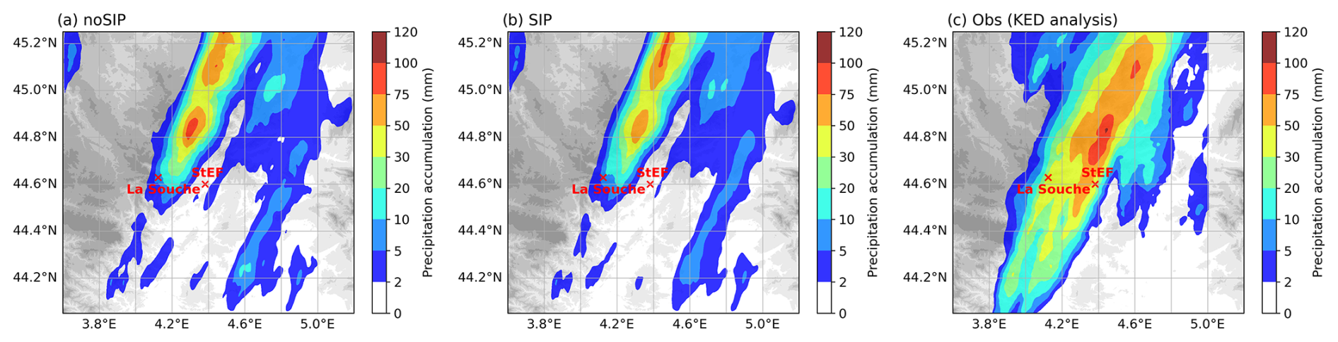
Figure 7 Precipitation accumulation (06:00–12:00 UTC) in the third domain for the (a) no-SIP simulation, (b) SIP simulation, and (c) observations using KED analysis. The locations of the La Souche and Saint-Étienne de Fontbellon (StEF) disdrometers are represented by red crosses.

To further investigate the precipitation properties, Fig. 8 presents the normalized frequency of the simulated and observed precipitation accumulation. First, in Fig. 8, both simulations give lower frequencies of precipitation accumulations greater than 15 mm compared to the observations (around 20 % less). Secondly, Fig. 8 shows that both simulations produce comparable precipitation frequencies below 40 mm, while above this value, the SIP simulation predicts less precipitation. As a result, the SIP simulation results in 8 % less total precipitation and 20 % less heavy precipitation exceeding 40 mm compared to the no-SIP simulation. Similar conclusions are found for the deep convective cloud case of Grzegorczyk et al. (2025b), where the total precipitation amount is reduced by 15 % and the accumulated precipitation exceeding 40 mm is reduced by 25 % due to the presence of SIP. The effect of SIP on precipitation is therefore more pronounced for the deep convective case studied in Grzegorczyk et al. (2025b) compared to the present study. This could be due to the fact that the production rates of ice crystals by SIP (Fig. 5) are here 10 times lower than those in Grzegorczyk et al. (2025b).

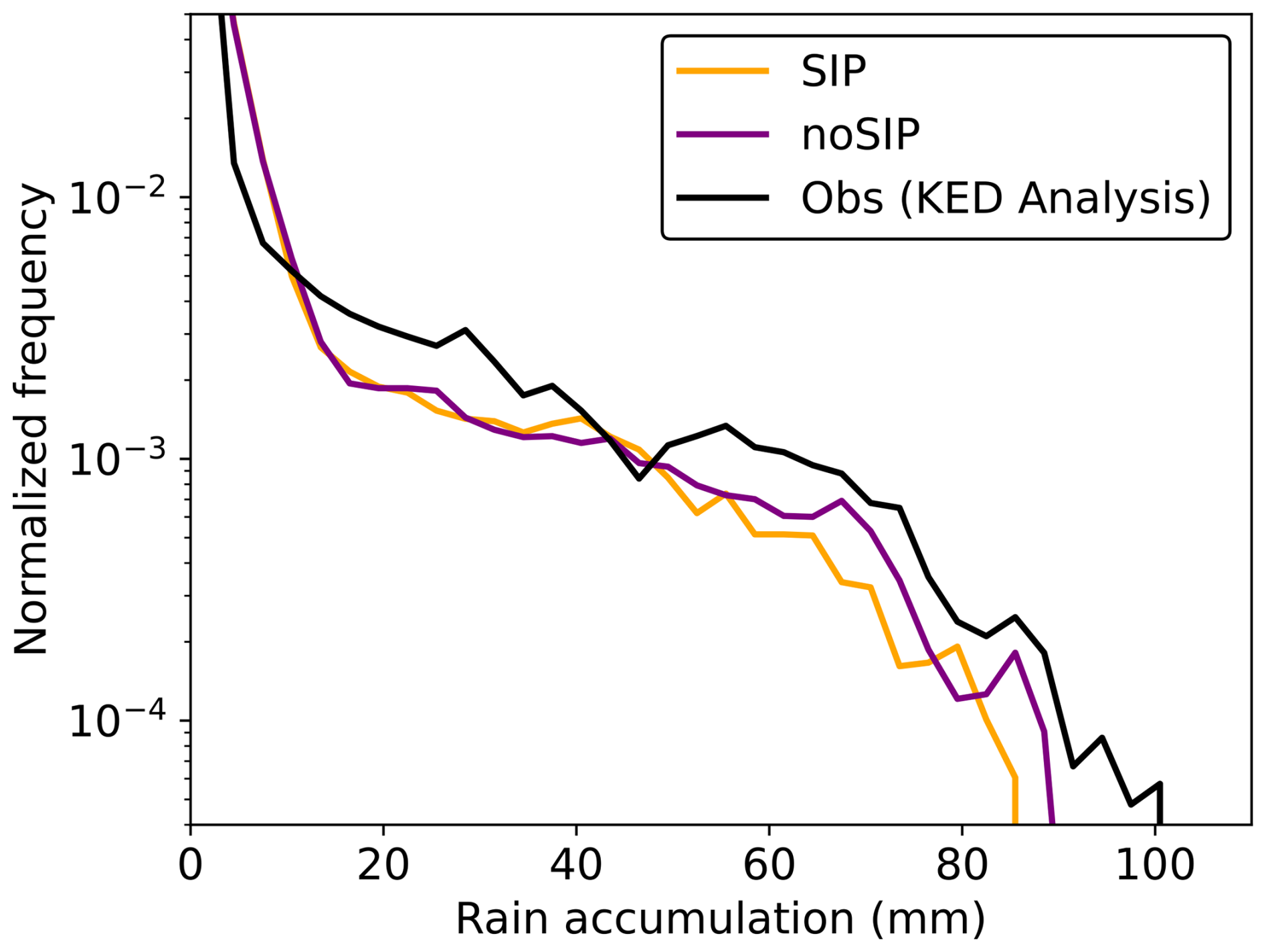
Figure 8 Normalized frequency of simulated (no SIP and SIP) and observed (KED analysis) rain accumulation from 06:00 to 12:00 UTC.

Several other studies have found that SIP reduces precipitation: Dedekind et al. (2021) report a decrease in regions with invigorated precipitation rates for alpine mixed-phase orographic clouds; Phillips et al. (2017b) show a reduction in accumulated precipitation of 20 % to 40 % due to BRK for a convective storm; similarly, Han et al. (2024) indicate a reduction in surface precipitation by up to 20 % for a deep convective cloud case; and Hoarau et al. (2018) show a decrease in surface precipitation depending on the intensity of the BRK process for a thunderstorm. Conversely, two other studies report the opposite effect: Sullivan et al. (2018) find that SIP enhances precipitation rate in convective regions of a cold frontal system, and Georgakaki et al. (2022) depict an increase in mean surface precipitation by up to 30 % due to SIP for wintertime alpine mixed-phase clouds.

4.2.2 Drop size distributions

Figure 9 shows the mean drop size distributions (DSDs) from the two disdrometers (locations indicated in Fig. 7) and those from the no-SIP and SIP simulations. However, as precipitation is absent in the southern part of the third domain in Fig. 7, it is not possible to directly compare the simulated DSDs with the disdrometer measurements at their exact locations. Consequently, to perform the comparison, we selected model grid points at the surface within the area presented in Fig. 1b, whose elevations were close (within ±150 m) to those of the disdrometers. Disdrometer data were taken at 08:30 UTC for StEF and 09:40 UTC for La Souche. These times correspond to the strong-precipitation periods recorded by the disdrometers, as described in Sect. 2.2. Furthermore, mean observed and modeled DSDs are compared for rain intensities between 10 and 20 mm h⁻¹. This comparison method is similar to the one used in Kagkara et al. (2020).

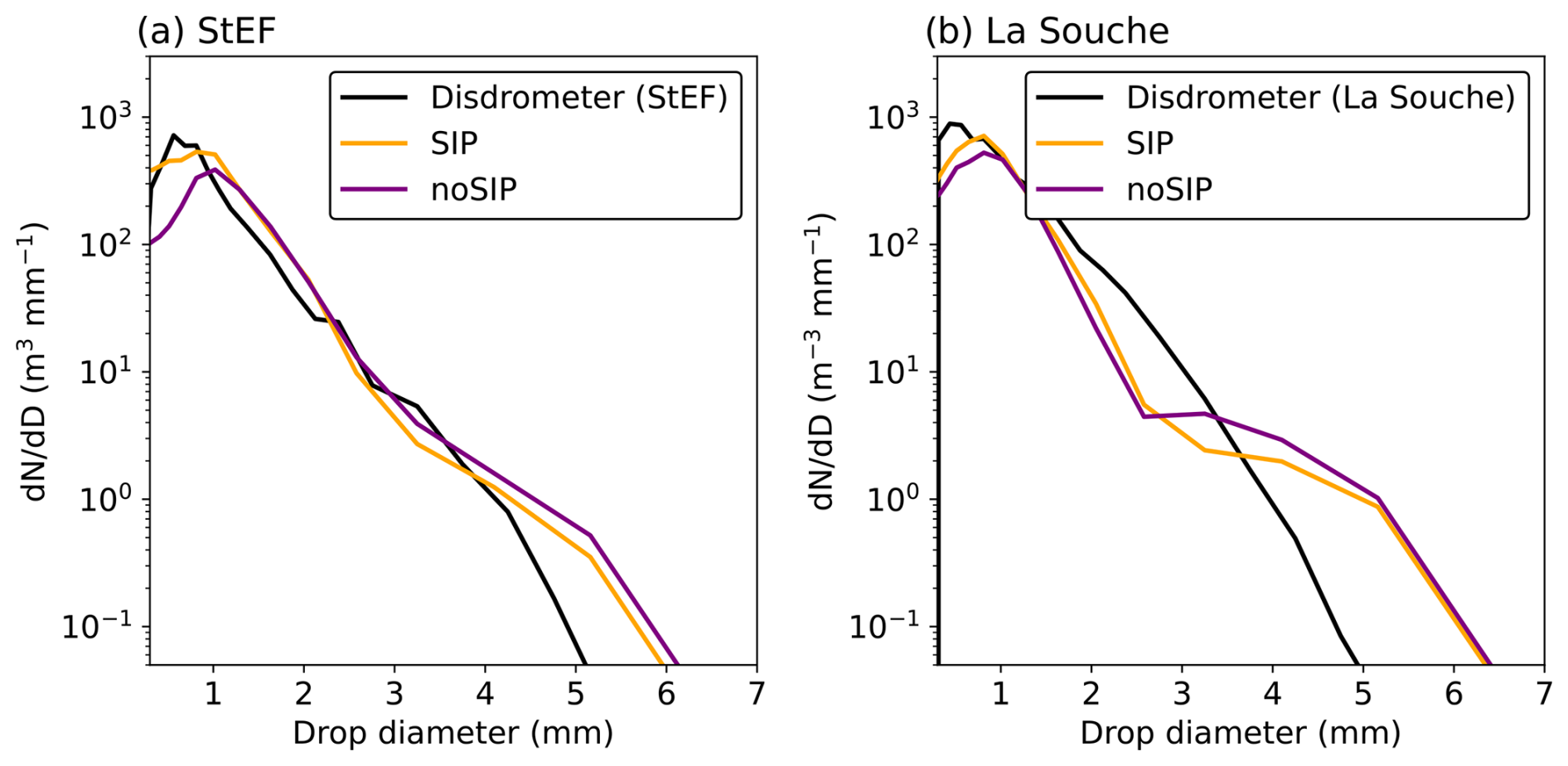
Figure 9 Mean drop size distributions (DSDs) for no-SIP and SIP simulations compared to disdrometer observations at (a) Saint-Étienne de Fontbellon (StEF) and (b) La Souche for rain intensities between 10 and 20 mm h⁻¹. Model results are taken at elevations close (within ±150 m) to those of the distrometer stations. Disdrometer data were taken at 08:30 UTC for StEF and 09:40 UTC for La Souche.

For both disdrometers (Fig. 9a and b), the SIP simulation exhibits a higher number of drops with D < 2 mm, while the number of larger drops with D > 3 mm decreases in comparison to the no-SIP simulation. Although including SIP gives a DSD that is in better accordance with the observations compared to no SIP, it does not sufficiently match the observations. Indeed, the slopes of both simulated DSDs show a sudden change at 3 mm in diameter, resulting in an overestimation of the number of drops larger than 4 mm compared to the observations. For La Souche (Fig. 9b), even if SIP increases the number of small drops, the simulated DSD peaks at 7 × 10² m⁻³ mm⁻¹ for 0.80 mm drops, whereas the observed DSD peaks at 10 × 10² m⁻³ mm⁻¹ for 0.45 mm drops.

The change in the DSD slope at 3 mm and the associated overestimation in the number of larger drops may arise from an inappropriate representation of the coalescence or collision efficiency. The coalescence efficiency currently implemented in DESCAM for D > 0.8 mm is derived from Beard and Ochs (1995), and the collision efficiency is based on Hall (1980). Furthermore, the simulations performed in this study were conducted without considering the collisional raindrop breakup process (Low and List, 1982) (currently under implementation), which might explain the underestimation of the small-drop number concentration in our results. Even if the total rain amounts are reasonably represented in our simulations, a detailed investigation of drop collision, coalescence, and breakup processes needs to be done in DESCAM to address the misrepresentation of the DSDs.

Figure 10a and b show the mean vertical profile of the total water content (TWC) for the SIP and no-SIP simulations obtained in mass bins (i.e., drop or melted ice diameter) of the distribution used in DESCAM (see Sect. 3) to described the hydrometeors. The TWC of the SIP simulation (Fig. 10a) reaches a maximum (up to 0.1 g m⁻³) for hydrometeor sizes close to 1 mm at 4 km altitude, whereas for the no-SIP simulation (Fig. 10b), this maximum occurs for larger particle sizes (around 4 mm). To further highlight this change in mass distribution of ice and liquid water, Fig. 10c shows the differences in TWC between the SIP (Fig. 10a) and no-SIP (Fig. 10b) simulations. Figure 10c confirms that SIP processes cause a shift in condensed mass towards smaller particle sizes in the cloud mixed phase (up to −20 °C). This shift may result from the increased concentration of small ice crystals (< 2 mm melted equivalent diameter), which triggers riming and vapor deposition (as presented in Fig. 8 of Grzegorczyk et al., 2025b), thereby enhancing the TWC at smaller particle diameters. Furthermore, the ice mass resulting from vapor deposition or riming is distributed over a larger number of ice crystals when SIP is active, leading to competition between crystals across different sizes, as highlighted by Phillips et al. (2017b). This could explain why Fig. 10c shows a smaller amount of condensed mass in the SIP simulation for particles larger than 3 mm compared to the no-SIP simulation.

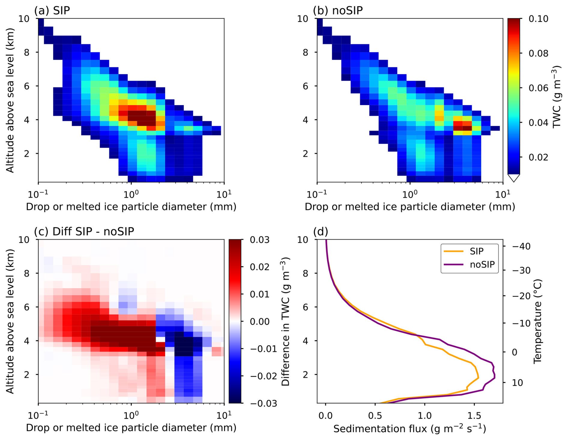
Figure 10 Mean total water content (TWC) as a function of the altitude and drop diameter or melted ice particle diameter in the (a) SIP and (b) no-SIP simulations. The differences between panel (a) and panel (b) are illustrated in panel (c). Sedimentation fluxes of the SIP and no-SIP simulations as a function of the altitude are shown in panel (d).

Figure 10c shows that the TWC shift is also present in the liquid phase (T > 0 °C below 3.7 km) for the same particle masses (or equivalent melted diameters) as those of the overlying mixed-phase region with maxima at 2 mm and minima at 4 mm. The TWC differences are visible from the melting layer to the ground, which is consistent with the differences in DSDs obtained in SIP and no SIP (Fig. 9). One reason for the shift in the liquid mass distribution is certainly a consequence of the melting of the numerous smaller ice crystals present in the SIP simulation. In addition, the increased number of small drops (< 3 mm) in the SIP case could enhance drop condensation at smaller diameters, while reducing it at larger diameters due to competition between drops, as previously mentioned for ice crystals.

Figure 10d shows the vertical profile of the sedimentation fluxes of ice crystals and drops. In Fig. 10d, sedimentation is found to be up to 15 % lower in the SIP case compared to the no-SIP case at altitudes lower than 5 km. Although the mean LWC profile is similar between no SIP and SIP (Fig. 3b), the shift in condensed mass distribution toward smaller diameters in the SIP simulation (Fig. 10c), along with the fact that small drops fall more slowly than larger ones, probably explains the reduction in the sedimentation flux (Fig. 10d) and the precipitation accumulation in the SIP simulation (Fig. 8). Additionally, the reason for the stronger reduction in heavy precipitation (20 % for rainfall accumulation > 40 mm) by SIP compared to total precipitation may be due to the fact that intense-rainfall events are often associated with deep convection and high total water content (TWC), which are favorable conditions for SIP (see Korolev et al., 2020).

5 Conclusions

This study examines how secondary ice production (SIP) influences the cloud and rain microphysical properties of the IOP7a heavy-precipitation event encountered during the HYMEX campaign, which took place in September 2012 in southern France over the Cévennes–Vivarais mountainous region. Numerical experiments with SIP switched on and off (SIP and no-SIP simulations) are conducted using the 3D bin microphysics scheme DESCAM. The SIP simulation encompasses the Hallett–Mossop (HM), fragmentation due to ice–ice collision (BRK), and fragmentation of freezing drop (DS) processes. First, the simulated mixed-phase properties are compared to in situ aircraft observations obtained from the optical array 2DS probe, optical array PIP, and CDP. Secondly, the influence of SIP on rainfall properties is evaluated by comparing simulations to ground-based observations, including disdrometer and quantitative precipitation estimates. Finally, the physical mechanisms driving the changes in rainfall properties are examined in detail.

Our results show that including SIP increases the mean concentration of ice crystals (N_ice) from 0 to −20 °C, reaching up to 60 L⁻¹ at 4.5 km, which is 30 times higher than that of the no-SIP simulation. The simulated particle size distribution (PSD) of ice crystals from the SIP simulation aligns well with the observed PSD from the 2DS probe and PIP, showing an increase in N_ice for ice crystals smaller than 2 mm diameter compared to the no-SIP case. However, the number of ice crystals near 200 µm (mode of the PSD) is slightly underestimated in the SIP simulation, which might explain why N_ice is in some cases lower than measurements, peaking up to N_ice = 100 L⁻¹.

Modeling results indicate that the Hallett–Mossop (HM) process gives the highest production rate of ice crystals at −5 °C, while ice–ice breakup (BRK) is 4 times lower than HM at this temperature but more efficient across a broader altitude range (up to −25 °C). Overall, for temperatures warmer than −30 °C, the SIP simulation shows that 38 % of ice crystals are generated by HM, 59 % by BRK, and only 2 % and 1 % by drop shattering (DS) and heterogeneous nucleation.

Observations from the 2DS probe and CDP showed an increase in particle concentration below 100 µm, consistent with the presence of liquid droplets in the model. Indeed, an analysis of the 2DS probe images using a convolutional neural network (CNN) to classify hydrometeor types with diameters > 300 µm shows that drops represent less than 10 % of hydrometeors. Furthermore, the SIP simulation reveals a reduction in the number fraction of drops (with D > 300 µm), leading to better agreement with the observed drop fraction retrieved from the CNN classification. However, for temperatures colder than −20 °C, SIP appears to reduce the droplet number concentration too much compared with the CDP measurements and the results of the CNN classification. It is important to note that the changes in liquid and ice partitioning caused by SIP could significantly influence the radiative properties of mixed-phase clouds (Matus and L'Ecuyer, 2017).

Compared to the results of the quantitative precipitation estimates derived by the method of Boudevillain et al. (2016), the no-SIP and SIP simulations both underestimate the total amount of precipitation. This result is similar to that of the two previous studies on the HYMEX IOP7a case conducted with DESCAM (Arteaga et al., 2020; Kagkara et al., 2020). Additionally, the drop size distributions (DSDs) of the SIP and no-SIP simulations show an overestimation of raindrops larger than 4 mm and an underestimation of raindrops smaller than 3 mm compared to the disdrometer observations.

When SIP is included, the total precipitation amount is reduced by 8 %, while strong-rainfall accumulation exceeding 40 mm decreases by 20 %. Additionally, including SIP leads to a rise in drop numbers smaller than 2 mm and a reduction in drop numbers larger than 3 mm. By analyzing the vertical structure of the total water content (TWC) and the corresponding mass size distributions, we find that SIP induced a shift of the TWC mass toward smaller particle diameters. This effect seems to be induced by the high concentration of ice crystals produced by SIP, which triggers riming or vapor deposition at smaller diameters. As a result of the competition between small and large ice crystals, less mass condenses into larger ice crystals when SIP is active. A similar shift in TWC is observed in the liquid phase, coming from the melting of ice particles. As liquid water mass shifts toward smaller drops which fall more slowly than large ones, the sedimentation flux becomes reduced (by up to 15 %), further diminishing precipitation accumulation. Given that SIP is particularly effective in convective conditions, it might explain why its impact is especially pronounced for heavy rainfall (20 % reduction for rainfall exceeding 40 mm).

The effects of SIP depicted here are similar to those presented in Grzegorczyk et al. (2025a, b) for an idealized tropical deep convective cloud corresponding to the HAIC/HIWC campaign (Fontaine et al., 2020; Hu et al., 2021). However, in the present study, the HM process plays a more important role, while the reduction in precipitation accumulation is slightly lower compared to in Grzegorczyk et al. (2025b). Therefore, the convection depth and the cloud type seem to influence the importance and effect of SIP processes.

This study demonstrates the importance of SIP for the cloud mixed phase and its significant effect on the rainfall properties of a heavy-precipitation event. While SIP improves agreement between simulated and observed DSDs, rain processes, such as drop collision, coalescence, and breakup, need to be reevaluated in DESCAM to better fit with the observations. Furthermore, an accurate quantification of SIP processes is still lacking, and the current results should be interpreted with caution. Future laboratory and field studies should focus on better quantifying SIP processes to improve parameterizations used in microphysical schemes.

Appendix A: Parameterization of secondary ice production in DESCAM

A1 Hallett–Mossop (HM)

The number of ice fragments generated by the Hallett–Mossop process in DESCAM is defined by

$$\begin{array}{}\text{(A1)}& {\displaystyle \frac{\partial n_{\mathrm{I}}\left(m_{\mathrm{frag}}\right)}{\partial t}}=N_{\mathrm{HM}}\cdot \text{fct}\left(T\right)\cdot \left({\displaystyle \frac{\partial m_{\mathrm{r}}\left(m\right)}{\partial t}}\right),\end{array}$$

with n_I denoting the number of ice particles, m_frag the fragment mass, and m_r(m) the newly accreted rime mass from droplets larger than 24 µm in diameter and with mass m. m_r(m) is calculated from the stochastic equation solution scheme of Bott (1998), which provides the mass gained by ice particles that accreted droplets (see Eq. 1 of Grzegorczyk et al., 2025a). N_HM is the number of fragments produced at −5 °C, which is set to 350 mg⁻¹, as found in Hallett and Mossop (1974). The temperature dependency function fct(T) comes from Eq. (72) of Cotton et al. (1986), based on the experiments of Hallett and Mossop (1974). fct(T) is set to be equal to 1 at −5 °C and to linearly decrease to 0 at −3 and −8 °C.

The mass of ice fragments m_frag is assumed to depend on the parent drop mass (based on the observations of Choularton et al., 1980) and is given by

$$\begin{array}{}\text{(A2)}& m_{\mathrm{frag}}\left(m\right)=min\left(\mathrm{0.015}\times m,\mathrm{1.71}\times {\mathrm{10}}^{-\mathrm{8}}\right),\end{array}$$

with m denoting the mass of the accreted drop (in g).

A2 Drop shattering during freezing (DS)

DESCAM considers drop shattering during freezing from two modes, which are presented in Phillips et al. (2018). Mode 1 is activated in DESCAM when large drops collect less massive ice particles or during heterogeneous drop freezing. The number of drops that freeze upon collision with less or more massive ice particles is determined from the stochastic equation solution scheme of Bott (1998), while the number of droplets frozen by heterogeneous ice nucleation is calculated from the Hiron and Flossmann (2015) method, which is implemented in DESCAM (see Eq. 4 of Grzegorczyk et al., 2025a).

The total number of ice fragments for each frozen drop generated by mode 1 is given by

$$\begin{array}{}\text{(A3)}& {\displaystyle \frac{\partial n_{\mathrm{I}}\left(m_{\mathrm{frag}}\right)}{\partial t}}=N_{\mathrm{DS}}(m,T)\cdot {\left({\displaystyle \frac{\partial n_{\mathrm{D}}\left(m\right)}{\partial t}}\right)}_{\mathrm{freeze}},\end{array}$$

where m_frag is the mass of the fragments, and N_DS(m,T) is the total number of fragments for one frozen drop which is calculated from Eq. (1) of Phillips et al. (2018) as follows:

$$\begin{array}{}\text{(A4)}& N_{\mathrm{DS},\mathrm{1}}=F\left(D\right)\mathrm{\Omega }\left(T\right)\left[{\displaystyle \frac{\mathit{\zeta }{\mathit{\eta }}^{\mathrm{2}}}{(T-T_{\mathrm{0}}{)}^{\mathrm{2}}+{\mathit{\eta }}^{\mathrm{2}}}}+\mathit{\beta }T\right],\end{array}$$

with T denoting the drop temperature and D the drop diameter. The two thresholds Ω(T) and F(D) are used to activate fragmentation smoothly from −3 to −6 °C and from drop sizes of D = 50 to 60 µm. The parameters T₀, β, ζ, and η that depend on drop size are fitted in Phillips et al. (2018) based on an extensive laboratory experiment dataset.

Furthermore, from the total number of fragments (Eq. A4), Phillips et al. (2018) distinguish between small and large fragments. The small fragments are to be 10 µm in size, and their number is given by $N_{\mathrm{DS},\mathrm{1}}^{\mathrm{small}}=N_{\mathrm{DS},\mathrm{1}}-N_{\mathrm{DS},\mathrm{1}}^{\mathrm{big}}$. The large-fragment number $N_{\mathrm{DS},\mathrm{1}}^{\mathrm{big}}$ formed from mode 1 is

$$\begin{array}{}\text{(A5)}& N_{\mathrm{DS},\mathrm{1}}^{\mathrm{big}}=min\left\{F\left(D\right)\mathrm{\Omega }\left(T\right)\left[{\displaystyle \frac{{\mathit{\zeta }}_B{\mathit{\eta }}_B^{\mathrm{2}}}{{\left(T-T_{B,\mathrm{0}}\right)}^{\mathrm{2}}+{\mathit{\eta }}_B^{\mathrm{2}}}}+{\mathit{\beta }}_{B}T\right],N_{\mathrm{DS},\mathrm{1}}\right\}.\end{array}$$

The parameters of Eq. (A5) for large fragments represent the same quantities as the total number of fragments in Eq. (A4). The large-fragment mass is set to be $\mathrm{1}/\mathrm{2.5}$ times the mass of the parent drop.

Mode 2 occurs during collision of drops with more massive ice particles. In Phillips et al. (2018), the number of ice fragments formed via mode 2 is expressed by

$$\begin{array}{}\text{(A6)}& N_{\mathrm{DS},\mathrm{2}}=\mathrm{3}\mathrm{\Phi }\cdot \left[\mathrm{1}-f\left(T\right)\right]\cdot max\left(\text{DE}-{\text{DE}}_{\mathrm{crit}},\mathrm{0}\right),\end{array}$$

where DE = $\frac{K_{\mathrm{0}}}{\mathit{\sigma }\mathit{\pi }{D}^{\mathrm{2}}}$ is the dimensionless energy that is defined by the ratio between collision kinetic energy and the drop surface tension, DE_crit = 0.2 represents the threshold of DE for the onset of drop splashing, and f(T) is the frozen fraction of the drop that depends on temperature. Φ is the fraction of ice fragment regarding the total number of fragments (liquid and ice). We consider that Φ = 0.3, which is based on the experimental study of James et al. (2021). Furthermore, the mass of the fragments is set to be 1000 times smaller than the mass of the parent drop, as indicated in Phillips et al. (2018).

A3 Fragmentation due to ice–ice collisions (BRK)

In DESCAM, the rate at which ice particles collide without sticking and may therefore break is described by the stochastic breakup equation (Eq. 14 in Grzegorczyk et al., 2025a) and is treated within the Bott (1998) scheme.

The number of fragments generated per collision is based on the formulation of Phillips et al. (2017a) but using the experimental results of the laboratory study of Grzegorczyk et al. (2023). The number of fragments of mass m^′′ produced from the fragmentation of the ice particle of mass m due to the collision with m^′ is given by

$$\begin{array}{}\text{(A7)}& N_{\mathrm{BRK}}\left(m^{\prime \prime };m^{\prime },m\right)=N_{\mathrm{BRK}}^{\mathrm{tot}}(m,m^{\prime })\cdot P\left(m,m^{\prime \prime }\right).\end{array}$$

$P(m,m^{\prime \prime })$ is the number density distribution that gives the probability to generate a fragment of mass m^′′ from the total number of fragments $N_{\mathrm{BRK}}^{\mathrm{tot}}(m,m^{\prime })$ during the fragmentation of an ice particle of mass m. The total number of fragments is determined from the theory of Phillips et al. (2017a) by

$$\begin{array}{}\text{(A8)}& \begin{array}{rl}{N}_{\mathrm{BRK}}^{\mathrm{tot}}\left(m,m^{\prime }\right)& =\mathit{\alpha }\left(m,\mathit{\varphi }\right)A_M\left(T,\mathit{\varphi }\right)\\ & \left(\mathrm{1}-\exp {\left(-{\displaystyle \frac{C\left(\mathit{\varphi }\right)K_{\mathrm{0}}\left(m,m^{\prime },\mathit{\varphi },{\mathit{\varphi }}^{\prime }\right)}{\mathit{\alpha }(m,\mathit{\varphi })A_M(T,\mathit{\varphi })}}\right)}^{\mathit{\gamma }}\right).\end{array}\end{array}$$

α(m,ϕ) is the smallest area of the two colliding ice particles (in m²), A_M(T,ϕ) is the number density of breakable asperities on ice particles per unit area (in m⁻²), C(ϕ) is the asperity–fragility parameter (in J⁻¹), $K_{\mathrm{0}}(m,m^{\prime },\mathit{\varphi },{\mathit{\varphi }}^{\prime })$ is the collision kinetic energy (CKE), γ is a shape parameter, and ϕ and ϕ^′ are the rime fractions of the colliding ice particles.

The A_M(T,ϕ), C(ϕ), and γ parameters are determined from the experimental results of Grzegorczyk et al. (2023) for three collision types. Results of graupel–snowflake collisions are employed for the breakup of ice particles with ϕ < 0.5, while for ϕ > 0.5 (i.e., rimed particles), graupel–graupel and graupel–graupel with dendrite results are used and interpolated as a function of the supersaturation with respect to ice (S_i). We employ this supersaturation dependency as graupel–graupel collisions are performed in an environment without any vapor deposition (i.e., S_i is supposed to be close to zero), whereas graupel–graupel with dendrite collisions are done in a high-supersaturation environment (S_i = 0.23). The parameters of Eq. (A8) for −15 °C are given in Table A1.

Table A1 Parameters used in DESCAM (at −15 °C) for the fragmentation due to the ice–ice collision in the parameterization of Phillips et al. (2017a). These parameters are derived from three types of collision experiments performed in the laboratory study of Grzegorczyk et al. (2023). For ϕ < 0.5, parameters corresponding to graupel–snowflake collisions are used, and for ϕ > 0.5, an interpolation between graupel–graupel and graupel–dendrite collision parameters is done as a function of the ice supersaturation S_i.

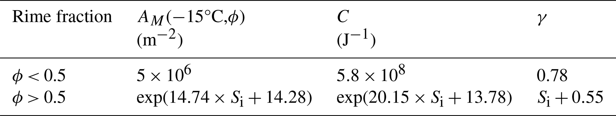
For temperatures that are different than −15 °C, a temperature dependency is considered for A_M(T,ϕ). It is based on the study by Takahashi et al. (1995) that investigated the effect of temperature on the number of fragments in a large-CKE regime. From the results of Takahashi et al. (1995), Phillips et al. (2017a) proposed a triangular temperature dependency, which is used here and is defined by

$$\begin{array}{}\text{(A9)}& \begin{array}{rl}{A}_M(T,\mathit{\varphi })& =A_M\left(-\mathrm{15}\mathrm{°}\mathrm{C},\mathit{\varphi }\right)\\ & \left({\displaystyle \frac{\mathrm{1}}{\mathrm{3}}}+max\left(\mathrm{0}.,{\displaystyle \frac{\mathrm{2}}{\mathrm{3}}}-{\displaystyle \frac{\mathrm{1}}{\mathrm{9}}}\times \left|\mathrm{15.0}+T\right|\right)\right),\end{array}\end{array}$$

with the temperature T in degrees Celsius. Regarding the fragment properties, the fragment mass distribution $P(m,m^{\prime \prime })$, derived from the fragment size distribution of Grzegorczyk et al. (2023), is used to distribute the fragments across the bins of DESCAM. It is defined by

$$\begin{array}{}\text{(A10)}& \begin{array}{rl}P\left(m,m^{\prime \prime }\right)& ={\displaystyle \frac{\mathrm{1}}{\mathit{\sigma }(m,\mathit{\varphi })\sqrt{\mathrm{2}\mathit{\pi }}}}\\ & \cdot \exp \left({\displaystyle \frac{\ln \left(m^{\prime \prime }\right)-\mathit{\mu }(m,\mathit{\varphi })}{\mathrm{2}\mathit{\sigma }(m,\mathit{\varphi }{)}^{\mathrm{2}}}}\right)\mathrm{\Delta }m,\end{array}\end{array}$$

with Δm denoting the width of mass bins. From the study of Grzegorczyk et al. (2023), which provides two distinct fragment size distributions for parent particles of different sizes (10 mm snowflakes and 4 mm graupel), we hypothesize that both the mode μ(m,ϕ) and the standard deviation σ(m,ϕ) of the distribution depend on the size of the parent ice particle. We therefore employ a linear interpolation to adjust μ(m,ϕ) and σ(m,ϕ) as a function of parent ice particle size of mass m as follows:

$$\begin{array}{}\text{(A11)}& \left\{\begin{array}{l}\mathit{\mu }(m,\mathit{\varphi })=min\left(\mathrm{3.95}\cdot D(m,\mathit{\varphi })-\mathrm{15.4},-\mathrm{9.475}\right)\\ \mathit{\sigma }(m,\mathit{\varphi })=min\left(\mathrm{1.28}\cdot D(m,\mathit{\varphi })+\mathrm{1.17},\mathrm{3.09}\right)\end{array}\right.,\end{array}$$

where D(m,ϕ) is the parent particle size in centimeters.