Water isotopic characterisation of the cloud–circulation coupling in the North Atlantic trades – Part 2: The imprint of the atmospheric circulation at different scales

Water vapour isotopes reflect the history of moist atmospheric processes encountered by the vapour since evaporating from the ocean, offering potential insights into the controls of shallow trade-wind cumuli. Given that these clouds, particularly their amount at the cloud base level, play an important role in the global radiative budget, improving our understanding of the hydrological cycle associated with them is crucial. This study examines the variability of water vapour isotopes at cloud base in the winter trades near Barbados and explores its connection to the atmospheric circulations ultimately governing cloud fraction. The analyses are based on nested COSMO_iso simulations with explicit convection during the EUREC⁴A (Elucidating the role of clouds-circulation coupling in climate) field campaign. It is shown that the contrasting isotope and humidity characteristics in clear-sky versus cloudy environments at cloud base emerge due to vertical transport on timescales of 4 to 14 h associated with local, convective circulations. In addition, the cloud base isotopes are sensitive to variations in the large-scale circulation on timescales of 4 to 6 d, which shows on average a Hadley-type subsidence but occasionally much stronger descent related to extratropical dry intrusions. This investigation, based on high-resolution isotope-enabled simulations in combination with trajectory analyses, reveals how dynamical processes at different timescales act in concert to produce the observed humidity variations at the base of trade-wind cumuli.

1 Introduction

The response of shallow trade-wind clouds to climate change is uncertain and known to contribute substantially to the spread of climate projections (e.g. Bony et al., 2015; Zelinka et al., 2017). Especially the cloud fraction at cloud base has been identified as a key variable influencing the spread of the modelled feedback of these clouds to climate change (Bony et al., 2017). To shed light on the mechanisms controlling cloud base cloud fraction in the trades, the field campaign EUREC⁴A (Stevens et al., 2021) was conducted in early 2020 near Barbados. The collected observations highlight the role of shallow mesoscale circulations (George et al., 2023) in driving the variability of vertical velocities at cloud base, which is an important control of cloud fraction at this level (Vogel et al., 2022). It remains to be investigated how these circulations, which have recently gained attention from the scientific community, shape the environment, particularly the distribution of humidity (Albright et al., 2022) and eventually cloud fraction.

Here, we are interested in using the abundance of heavy stable water vapour isotopologues as tracers of cloud microphysical processes, as well as turbulent and convective mixing. Heavy stable water vapour isotopologues (hereafter isotopes) are water molecules containing a heavy hydrogen (¹H²H¹⁶O or HDO) or oxygen atom (¹H₂¹⁸O). Compared to their light counterpart (¹H₂¹⁶O), they have lower saturation vapour pressures and lower diffusion velocities. This implies that the heavy water molecules preferably stay in the condensed phase, where they establish stronger intermolecular bonds compared to their lighter counterpart (equilibrium fractionation). Furthermore, the near-surface humidity gradient leads to a differentiation in the relative concentration of the two heavy isotopes (¹H²H¹⁶O and ¹H₂¹⁸O) due to their differences in diffusivity (non-equilibrium fractionation). This results in a change in the relative abundance of heavy-to-light isotopes during phase transitions. The isotopic composition of a water sample is typically assessed with the δ value for ²H and ¹⁸O, respectively:

$$\begin{array}{}\text{(1)}& {\displaystyle }{\mathit{\delta }}^{\mathrm{2}}\text{H}\left[\mathrm{‰}\right]=\left({\displaystyle \frac{{}^{\mathrm{2}}{R}_{\mathrm{sample}}}{{}^{\mathrm{2}}{R}_{\mathrm{VSMOW}}}}-\mathrm{1}\right)\cdot \mathrm{1000},\text{(2)}& {\displaystyle }{\mathit{\delta }}^{\mathrm{18}}\text{O}\left[\mathrm{‰}\right]=\left({\displaystyle \frac{{}^{\mathrm{18}}{R}_{\mathrm{sample}}}{{}^{\mathrm{18}}{R}_{\mathrm{VSMOW}}}}-\mathrm{1}\right)\cdot \mathrm{1000}.\end{array}$$

The R in the equations above stands for the atomic ratio of the concentration of the heavy to the light isotope, namely
${}^{\mathrm{2}}R=\frac{{[}^{\mathrm{2}}\text{H}]}{{[}^{\mathrm{1}}\text{H}]}$ and ${}^{\mathrm{18}}R=\frac{{[}^{\mathrm{18}}\text{O}]}{{[}^{\mathrm{16}}\text{O}]}$, in the water sample and the internationally accepted Vienna Mean Ocean Standard Water 2 (VSMOW; International Atomic Energy Agency, 2017). The relative variations of δ²H and δ¹⁸O due to non-equilibrium fractionation are assessed with the deuterium excess:

$$\begin{array}{}\text{(3)}& d\text{-excess}={\mathit{\delta }}^{\mathrm{2}}\text{H}-\mathrm{8}\times {\mathit{\delta }}^{\mathrm{18}}\text{O},\end{array}$$

which is a measure of the thermodynamic disequilibrium of the environment during phase transitions (e.g. Pfahl and Wernli, 2008). Due to these mechanisms, the abundance of heavy isotopes reflects the integral of all phase changes and mixing processes that occur along the flow. While the first-order isotope variable δ²H is sensitive to microphysical processes and mixing (Gat, 1996; Galewsky et al., 2016), the second-order isotope variable d-excess is sensitive to the thermodynamic conditions at the moisture source (Pfahl and Wernli, 2008; Aemisegger et al., 2021).

Part 1 of this companion paper showed that the horizontal variability of humidity and δ²H of vapour at the cloud base emerges from the circulation involving ascent within convective clouds and subsidence outside of clouds, which we will henceforth refer to as the cloud-relative circulation (Fig. 1a). Cloudy cloud base patches (representing the ascending branch) are moister and more enriched than the background conditions. In contrast, clear-sky, dry-warm cloud base patches (hereafter dry-warm patches; representing the descending branch) are drier and more depleted than the background conditions. This suggests, against the above-formulated expectations, that the isotopic characteristics of the two cloud base features mainly reflect vertical transport and are not primarily controlled by local microphysical or turbulent mixing processes, an aspect that we will investigate in more detail here in part 2 of this study.

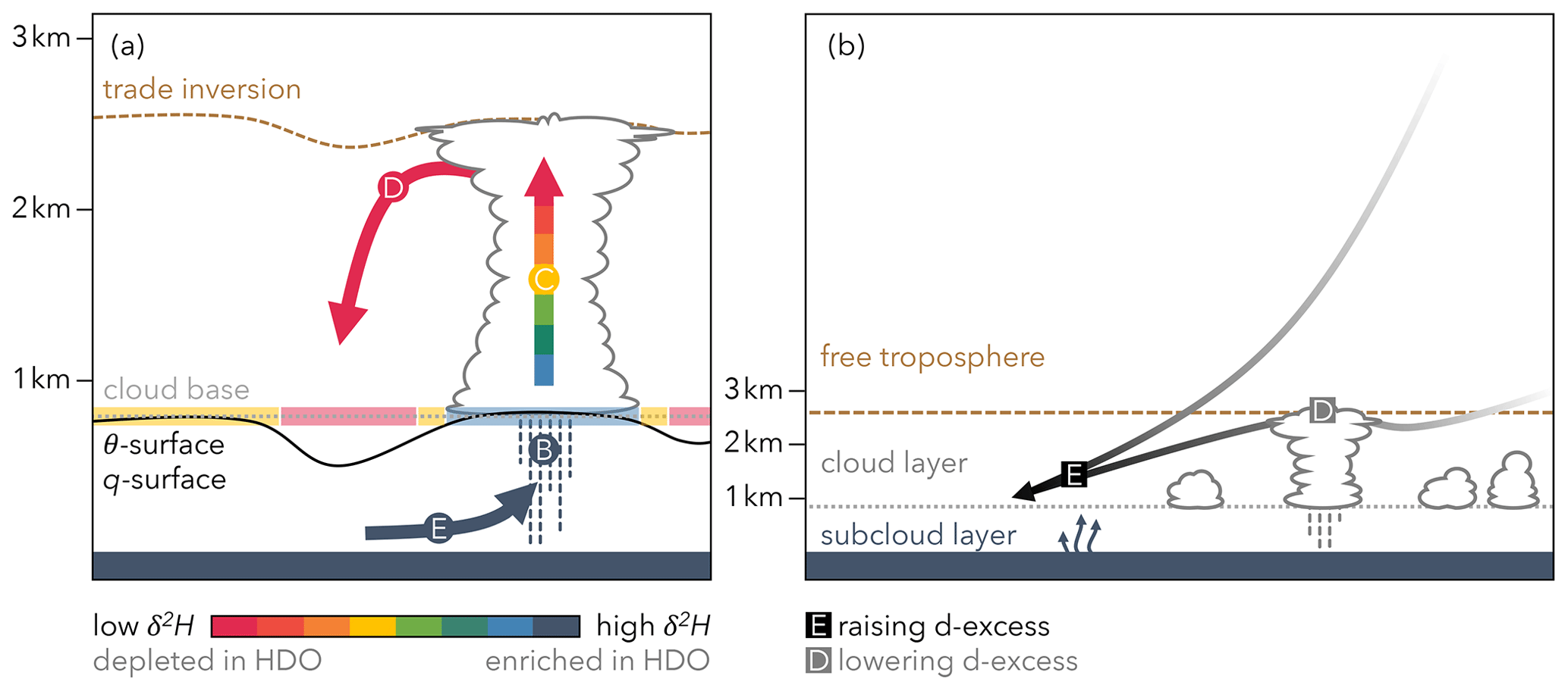
Figure 1 Idealised schematic of the processes affecting (a) the δ²H in vapour within the circulation associated with clouds and (b) the d-excess in vapour during large-scale transport. Shown are three atmospheric layers: the subcloud layer, the cloud layer, and the free troposphere. They are separated by the cloud base level (dotted grey) and the trade inversion (dashed brown). It is assumed that the two boundaries have an uneven topography in reality. However, in the simulations, cloud base is identified at a constant height. Therefore, the cloud (transparent blue in panel a), the clear (transparent yellow in a) and the dry-warm (transparent red in a) cloud base environments are defined at the flat cloud base (see Sect. 2.3 for the detailed definition of the three environments). (a) Within the cloud-relative circulation, air parcels (E) take up freshly evaporated (and therefore isotopically heavy) vapour (high δ²H; enriched in ¹H²H¹⁶O) from near the ocean surface; (B) may encounter below-cloud processes such as partial or full evaporation of hydrometeors and equilibration between vapour and liquid droplets, which can have a depleting or an enriching effect on the vapour (depending on the saturation level of the subcloud layer and the formation altitude of the rain; Aemisegger et al., 2015; Graf et al., 2019); and (C) will continuously lose heavy isotopes (lowering δ²H; depleted in ¹H²H¹⁶O) as soon as they reach the lifting condensation level and cloud and rain droplets are formed. Note that the temperature effect makes the fractionation stronger with increasing altitude. At any height, the now isotopically light air parcels may be detrained from the cloud into the surrounding clear-sky environment. Here, (D) the air parcel's vapour can get further depleted by mixing with vapour from above the trade inversion. (b) Within the large-scale circulation, air parcels can (E) take up moisture that is freshly evaporated from the ocean surface under non-equilibrium conditions and therefore have a relatively high d-excess (Pfahl and Wernli, 2008) and (D) get moistened through the detrainment of cloudy air from precipitating clouds and have a comparatively low d-excess (Noone, 2012; Thurnherr and Aemisegger, 2022).

In this paper, we establish a link between isotopes in the trade-wind region and the characteristics of atmospheric circulations. For this, we use three nested convection-resolving COSMO_iso simulations with different resolutions and air parcel backward trajectories from the cloud base environment. This data set, and the applied methods, is described in detail in Sect. 2. First, we look at processes on the subdaily timescale (Sect. 3). We investigate how convection drives the variability of humidity and isotopes in different cloud base environments (cloudy vs. dry-warm). Since convection in the trades has a clear diel cycle (Vial et al., 2019, 2021; Vogel et al., 2020), we use the diel cycle as a framework to answer the following question. Does the diel cycle of humidity and δ²H in different cloud base environments reflect the growth and decay of convection? Second, we test the hypothesis that the large-scale circulation transporting air into the trade-wind region leaves a distinct isotope signal in the cloud base vapour (Sect. 4). We thus address the following question. Which of the three variables, specific humidity (q), δ²H, and d-excess, is most strongly influenced by the large-scale circulation? In the conclusion, we combine the findings from the two research questions (Sect. 5).

2 Data and methods

2.1 Data sets

The data from three convection-resolving COSMO_iso simulations, described and evaluated in Villiger et al. (2023), are used. Convection resolving means that the convection schemes of the model (parameterising deep and shallow convection; see Tiedtke, 1989; Theunert and Seifert, 2006) were disabled. We have used the COSMO_iso model in this set-up in many previous studies (Dahinden et al., 2021; Diekmann et al., 2021; Thurnherr et al., 2021; de Vries et al., 2022), in which the comparison with isotope observations in various regions of the world has shown a good performance of the explicit convection set-up. Furthermore, previous analyses have shown that COSMO simulations at a range of resolutions (grid spacing ≤ 25 km) do not necessarily provide more realistic results in terms of radiation and precipitation patterns if shallow convection is parameterised (Vergara-Temprado et al., 2020).

For the three simulations used here, a 20 s model time step was applied, and hourly output was generated. The simulations differ in terms of domain as well as horizontal (10, 5, 1 km) and vertical (40, 60, 60 levels) grid spacings. These differences are summarised below (for more details, see Villiger et al., 2023, in particular their Fig. 2):

• COSMO_iso,10 km has a horizontal resolution of 0.1^∘, has 40 vertical levels, and covers most of the North Atlantic. Horizontal winds above 850 hPa in COSMO_iso,10 km were nudged towards a simulation performed with the global model ECHAM6-wiso (Cauquoin et al., 2019; Cauquoin and Werner, 2021), which also served as a source for initial, lateral, and top boundary conditions at 6-hourly intervals. A Rayleigh damping to the top boundary condition was used in the upper levels of the model domain. The ECHAM6-wiso simulation, itself, was nudged towards ERA5 (Hersbach et al., 2020) to reproduce the large-scale meteorological conditions of the simulated period. COSMO_iso,10 km covers the period from 6 January to 13 February 2020 of which the first 10 d are treated as spin-up and are not included in the analysis.

• COSMO_iso,5 km has a horizontal resolution of 0.05^∘, has 60 vertical levels, and covers a subset of the western North Atlantic, including the northern part of the South American continent. Initial and lateral boundary conditions originate from COSMO_iso,10 km at hourly time steps. The spectral nudging technique was identical to the first COSMO_iso simulation but nudged towards COSMO_iso,10 km horizontal winds above 850 hPa instead of ECHAM6-wiso. COSMO_iso,5 km covers the period from 20 January to 13 February 2020. All simulated days are included in the analysis.

• COSMO_iso,1 km has a horizontal resolution of 0.01^∘, has 60 vertical levels, and covers the focus area of the EUREC⁴A campaign's field activity. Initial and lateral boundary conditions originate from COSMO_iso,5 km at hourly time steps, and the spectral nudging was directed towards COSMO_iso,5 km wind data. COSMO_iso,1 km covers the period from 20 January to 13 February 2020, and all simulated days are taken into account for the analysis.

COSMO_iso,1 km and COSMO_iso,5 km are used to characterise the cloud-relative circulation (Sect. 3), and COSMO_iso,10 km is used to assess the large-scale circulation (Sect. 4). For this, air parcel backward trajectories are calculated with data from COSMO_iso,5 km and COSMO_iso,10 km using the Lagrangian analysis tool LAGRANTO (Wernli and Davies, 1997; Sprenger and Wernli, 2015, see detailed description of trajectory starting points in Sect. 2.4 and 2.5). LAGRANTO trajectories are based on the three-dimensional hourly wind fields of the respective data set, which do not resolve sub-grid-scale boundary layer processes. To alleviate this limitation, we compute a large set of trajectories. Note also that the COSMO_iso,10 km trajectories spend comparably little of their lifetime near the boundary layer, and the COSMO_iso,5 km trajectories are explicitly started from features that are dominated by subsidence and thus well characterised by the grid-scale winds.

2.2 Definition of cloud base

Cloud base is identified using the same procedure as in Villiger et al. (2023), which includes the following steps:

1. Vertical profiles at every grid point in the domain 54.5–61^∘ W and 11–16^∘ N are checked for cloud water content exceeding 10 mg kg⁻¹ (threshold for the detection of clouds used in Vial et al., 2019) at any model level below 1.3 km. The lowest model level meeting this criterion is taken as the cloud base of the respective vertical profile. If a given profile does not contain any clouds (i.e. does not meet the criteria), it is ignored in the subsequent step.

2. In order to extract cloud base conditions, we determine one representative cloud base model level for the domain 54.5–61^∘ W and 11–16^∘ N by calculating the median over the cloud base model levels identified for cloudy profiles in the previous step.

3. Steps 1 and 2 are repeated for every hourly time step of the simulated time period. The resulting time series of cloud base model levels can then be used to extract cloud base variables from the COSMO_iso simulations.

The hourly cloud base levels alternate between 783 and 970 m for COSMO_iso,10 km and change between three levels, i.e. 761, 914, and 1082 m, for COSMO_iso,5 km and COSMO_iso,1 km.

2.3 Definition of cloud base features

The COSMO_iso,1 km and COSMO_iso,5 km grid points at cloud base in the domain 54.5–61^∘ W and 11–16^∘ N are assigned to three categories representing features from the circulation associated with clouds, clear-sky regions with dry-warm anomalies, and clear-sky regions without dry-warm anomalies (see details in Villiger et al., 2023, note that here we do not differentiate between precipitating and non-precipitating clouds). The following definitions are applied to assign the data points to the three categories cloud, dry-warm, and clear:

• Cloud grid points are identified based on liquid cloud water content exceeding 10 mg kg⁻¹.

• Dry-warm grid points are identified by a positive anomaly in potential temperature (θ) and a negative anomaly in q. The anomalies are defined grid-point-wise by removing the daily cycle. For each grid point, the hour-of-the-day mean and standard deviation are calculated over the whole simulated period (20 January to 13 February 2020). Dry-warm grid points are then selected using the following criteria: $q_{i,t}<\stackrel{\mathrm{‾}}{q_{i,h\left(t\right)}}-\mathit{\sigma }\left(q_{i,h\left(t\right)}\right)$ and ${\mathit{\theta }}_{i,t}>\stackrel{\mathrm{‾}}{{\mathit{\theta }}_{i,h\left(t\right)}}+\mathit{\sigma }\left({\mathit{\theta }}_{i,h\left(t\right)}\right)$ (i denoting the grid points inside the evaluation domain, t the hourly time steps of the simulated period, h(t) the hour of the day corresponding to the time step t, and σ the standard deviation of the considered variable). We checked that these criteria exclusively select clear-sky grid points (i.e. liquid cloud water content below 10 mg kg⁻¹) without using an additional criterion for the liquid cloud water content. An overview of the number of identified dry-warm grid points per time step is given in Fig. 2, and an exemplary time step illustrating their spatial distribution is given in Fig. 3.

• The remaining clear-sky grid points (i.e. liquid cloud water content below 10 mg kg⁻¹ but no positive anomaly in θ combined with a negative anomaly in q) are categorised as clear.

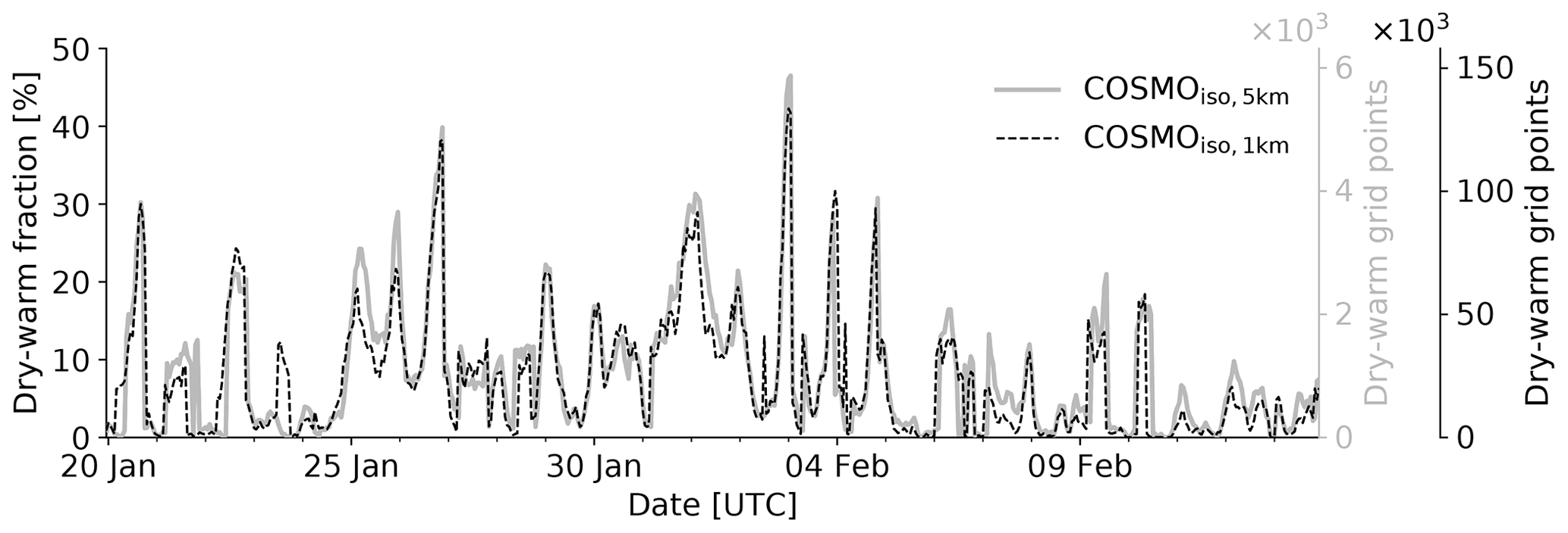
Figure 2 Hourly time series of fraction (left axis) and number (right axis) of cloud base grid points in the domain 54.5–61^∘ W and 11–16^∘ N categorised as dry-warm in COSMO_iso,5 km (grey continuous) and COSMO_iso,1 km (black dashed). In case of COSMO_iso,5 km, these cloud base grid points serve as starting points of the dry-warm backward trajectories (see text for details). The total numbers of cloud base grid points in the considered domain are 12 632 for COSMO_iso,5 km and 316 028 for COSMO_iso,1 km.

The reasoning behind the separation of dry-warm and clear grid points at cloud base into different categories stems from part 1 of this study. We assume that the characteristics of the dry-warm category result from coherent mesoscale subsidence and, therefore, can give insight into the downward branch of the cloud-relative circulation (sketched in Fig. 1). A dry-warm anomaly is expected at the cloud base level of the downward branch because (1) subsidence causes adiabatic warming (generating a warm anomaly at cloud base), and (2) a coherent mesoscale dry-warm anomaly ensures a certain distance from clouds and through this minimises the influence of mixing with moist air from surrounding clouds, thereby avoiding major impacts of evaporating cloud and rain droplets. Crucially, the absence of mixing and phase changes along the subsidence path leads to a conservation of the isotope signal in the vapour from the point at which it was detrained from the cloud down to cloud base. As shown in the exemplary time step in Fig. 3, our definition of dry-warm indeed applies to grid points that are well away from clouds and therefore are optimal to analyse the processes associated with subsidence alone, which we expect to be resolved in the simulations used here.

For the clear category, we assume that several processes (subsidence, turbulent mixing, and evaporation of cloud and rain droplets) impact its characteristics. Some of these, e.g. turbulent mixing, occur on shorter temporal and spatial scales than resolved by our backward trajectories based on hourly simulation output. Whether the two cloud base environments, clear and dry-warm, truly emerge due to different processes is assessed statistically using backward trajectories as described in the next section.

Although we have a special interest in the dry-warm category, it is important to remember that clear grid points at cloud base cover a much larger area. Namely, about 81 % of the cloud base grid points in COSMO_iso,1 km are categorised as clear and only about 8 % as dry-warm, considered over the whole simulated period. This means, for instance, that for the mass balance at cloud base, the clear category plays a more important role than the dry-warm one (knowing that at the cloud base level, local downward winds of similar magnitude prevail in both; see Villiger et al., 2023, their Fig. 15d).

2.4 Lagrangian characterisation of the cloud-relative circulation

To investigate the formation mechanism of the dry-warm patches at cloud base, we calculate 24 h backward trajectories. We start them at hourly time steps between 22 January and 13 February 2020 from all cloud base grid points identified as dry-warm in the domain 54.5–61^∘ W and 11–16^∘ N in the COSMO_iso,5 km simulation. Note that the number of dry-warm cloud base grid points varies from time step to time step (Fig. 2). Summed over all time steps, this results in a total of 568 124 dry-warm trajectories. Similarly, we start 24 h backward trajectories every hourly time step between 22 January and 13 February 2020 from 1000 randomly selected cloud base grid points identified as clear in the COSMO_iso,5 km simulation. We fix the number of clear trajectories for computational reasons, since about 9000 grid points are identified as clear every hourly time step (not shown). Summed over all time steps, this results in a total of 539 460 clear trajectories. The starting points of the dry-warm (red areas) and clear (yellow dots) backward trajectories are shown for an exemplary time step in Fig. 3d.

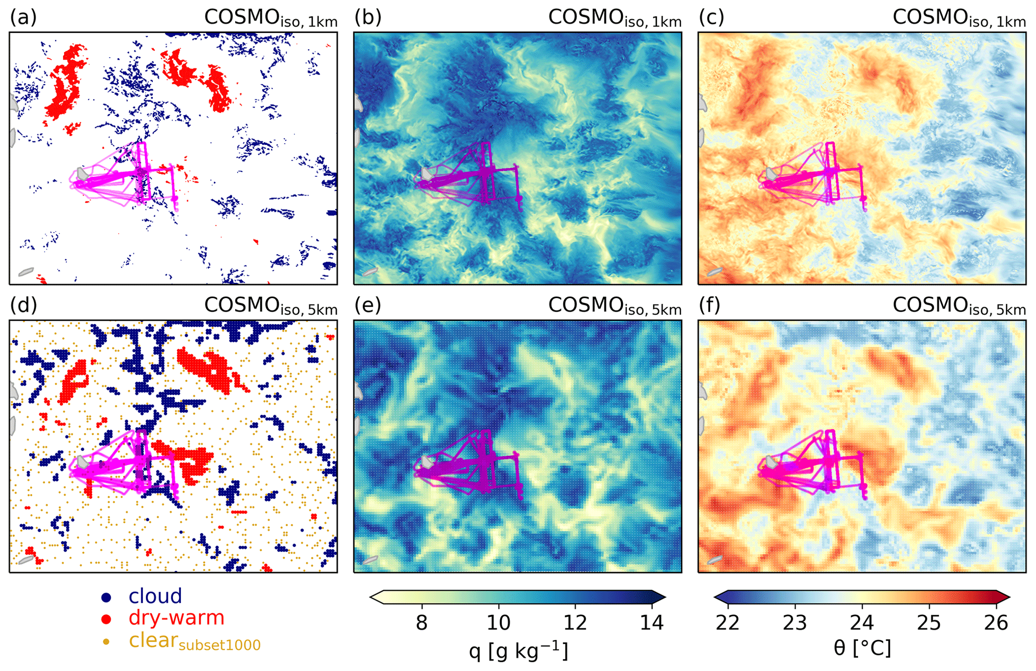
Figure 3 Spatial distribution of (a, d) cloud base grid points identified as cloud (blue), dry-warm (red), or clear (yellow; only a subset of 1000 randomly selected data points), (b, e) specific humidity (q), and (c, f) potential temperature (θ) at cloud base at 15:00 UTC on 2 February 2020. Shown is the data from (a–c) COSMO_iso,1 km and (d–f) COSMO_iso,5 km in the domain 54.5–61^∘ W and 11–16^∘ N. The fraction of grid points in the domain identified as dry-warm is (a) 3.3 % or (d) 4.3 %. (d) COSMO_iso,5 km backward trajectories (see text for details) are started from the red areas (representing all dry-warm cloud base grid points) and the yellow dots (representing 1000 randomly selected clear grid points at cloud base). For scale, the flight track of the aircraft ATR42 (Bony et al., 2022) during EUREC⁴A is shown in pink.

To learn about the overturning time and vertical depth of the cloud-relative circulation, we determine the altitude and time step, at which each air parcel was last located inside a cloud before arriving at cloud base (i.e. we perform a last point of saturation analysis; cf. Galewsky et al., 2016). For this, we check the cloud liquid water content along each trajectory and identify the last time step before arrival, when the cloud liquid water content exceeded 10 mg kg⁻¹ (sketch in Fig. 4). We refer to the air parcel's altitude at this time step as cloud detrainment altitude (Figs. 5c and 10a) and interpret it as the upper turning point of the circulation (where the air parcel is detrained from the cloudy updraught and starts to subside towards the surface). Note that only 58 % of the air parcels arriving in a dry-warm cloud base environment encounter a cloud during the previous 24 h. For air parcels arriving at clear grid points at cloud base, this value amounts to 79 %.

We limit the trajectories to 24 h because we want to isolate the coupling between the upward and downward branch of the circulation. Since the upward branch (i.e. convection) is known to have a clear diel cycle (Vial et al., 2019, 2021; Vogel et al., 2020, 2022), it is reasonable to look at the downward branch over the same time period. We use COSMO_iso,5 km for these trajectories because COSMO_iso,1 km has too small a domain to trace air parcels over several hours. We use the variables cloud detrainment altitude and time step in Sects. 3 and 5.

2.5 Lagrangian characterisation of the large-scale circulation

We calculate backward trajectories based on COSMO_iso,10 km data to evaluate the role of the large-scale circulation for the isotopic composition of vapour around cloud base in Sect. 4. A total of 138 trajectories, reaching 6 d backwards in time, are started every hour from 22 January to 13 February 2020, which is sufficient to capture the influence of a large-scale signal. The starting points are distributed over three vertical levels and horizontally spaced with a distance of 100 km in the domain 54.5–61^∘ W and 11–16^∘ N. The three vertical levels at 940, 920, and 900 hPa are chosen such that they bracket cloud base to take into account some variability in the cloud base level in the coarse resolution data set. Hereafter, the air parcel's arrival level is referred to as cloud base. Furthermore, we do not distinguish between different cloud base mesoscale features (as in Sect. 2.3 and 2.4), because we expect the large-scale circulation to modulate isotope signals at the large scale.

To distinguish between different large-scale flow patterns and to assess the coupling between large-scale flow and cloud base isotopes, we calculate the mean 1 h vertical displacement based on the change of altitude (${\stackrel{\mathrm{‾}}{\mathrm{\Delta }z}}_{X\mathrm{d}}$; sketch in Fig. 4) over different time windows ($X=\mathrm{1},\mathrm{\dots },\mathrm{6}$ d) for each trajectory. This variable is used in Sects. 4 and 5.

The sources of the moisture arriving in the EUREC⁴A domain and their associated conditions are characterised based on the algorithm developed by Sodemann et al. (2008) and using the COSMO_iso,10 km trajectories. In short, a trajectory-based water mass balance is computed and temporal changes in q along the backward trajectories are identified as uptakes if positive and rain events if negative. The weight of each uptake is determined according to its mass contribution to the final q at arrival by proportionally discounting the influence of uptakes happening before rain events underway. Moisture source conditions, in particular the relative humidity with respect to sea surface temperature (RH_SST), which is known to control the d-excess signal, were calculated as mass-weighted means using the weights of the individual uptakes (for more details, see Aemisegger et al., 2014).

3 Cloud base isotopes and the cloud-relative circulation

This section discusses how the cloud-relative circulation (Fig. 5) drives the diel cycle of isotopes in different cloud base environments (Fig. 6). For this, we analyse the temporal evolution of the isotope signals at the cloud base data points from COSMO_iso,1 km categorised as cloud, clear, and dry-warm (Sect. 2.3). In addition, we use COSMO_iso,5 km trajectories to derive an estimate of the rooting altitude of the subsiding branch of the cloud-relative circulation (cloud detrainment altitude; see Sect. 2.4). When combining these two data sets, it is important to know that the vertical velocities within cloud and dry-warm cloud base environments are stronger in COSMO_iso,1 km than in COSMO_iso,5 km. However, the diel cycles of vertical velocities in the two data sets are the same (not shown). We argue that we can use the variables characterising the cloud-relative circulation derived from the COSMO_iso,5 km trajectories, as our primary focus lies in discerning their variation (and not their absolute values) throughout the day and in understanding how this variation correlates with changes in cloud base isotopes.

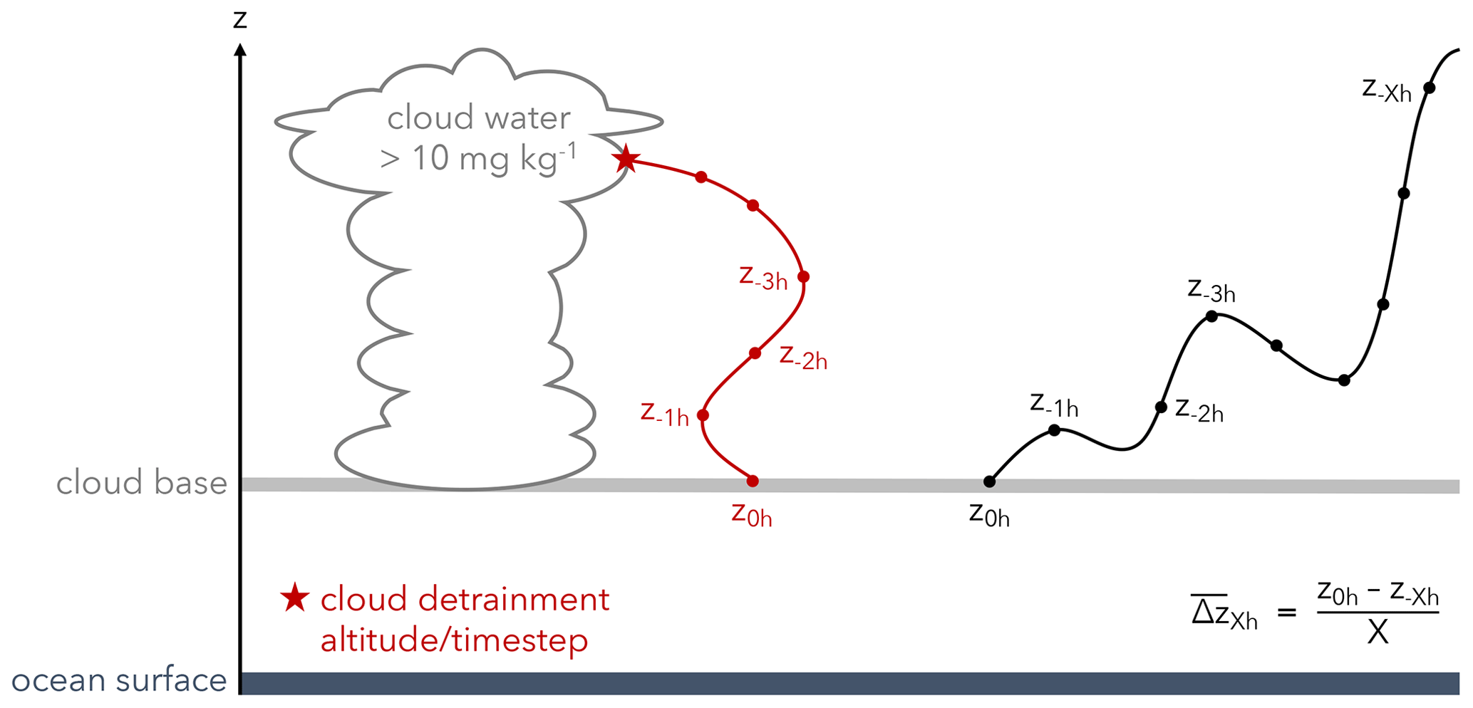
Figure 4 Schematic of two individual air parcel's backward trajectory started from cloud base. The red trajectory showcases the procedure to identify the cloud detrainment altitude and time step of the air parcel (red star). This procedure is applied to the COSMO_iso,5 km backward trajectories (Sect. 2.4). The black trajectory showcases the procedure to obtain the mean vertical displacement over a certain time period (${\stackrel{\mathrm{‾}}{\mathrm{\Delta }z}}_{-X\mathrm{h}}$), which is calculated for the COSMO_iso,10 km backward trajectories (Sect. 2.5). Here, z_0 h indicates the altitude from which the backward trajectory is started, and z_−1 h, z_−2 h, $z_{-\mathrm{3}\mathrm{h}},\mathrm{\dots },z_{-X\mathrm{h}}$ the altitude of the air parcel $\mathrm{1},\mathrm{2},\mathrm{3}\mathrm{h},\mathrm{\dots },X\mathrm{h}$ before arrival at cloud base, respectively. The altitude difference between z_0 h and z_−X h divided by the hours between the two considered time steps yields the mean altitude change over X h, i.e. ${\stackrel{\mathrm{‾}}{\mathrm{\Delta }z}}_{X\mathrm{h}}$. Note that if time periods longer than 24 h are considered, the notation is adapted to days instead of hours (i.e. ${\stackrel{\mathrm{‾}}{\mathrm{\Delta }z}}_{X\mathrm{d}}$).

Before we move on to exploring the potential coupling between the cloud-relative circulation and cloud base isotope signals, we have to briefly address the evaluation of the diel cycles with observations. The modelled diel cycles cannot be evaluated directly with observations due to the lack of available observations at cloud base in different environments (cloud, clear, dry-warm) over the entire day. Instead, an evaluation of the diel cycle from observations at a close-by land site along the east coast of Barbados (BCO site; see Bailey et al., 2023) has been done, which shows a good agreement with the model (Appendix A). The diel cycles of q and δ²H in clouds at cloud base are in phase with and of the same amplitude as the respective variable at the coastal site. A slight delay in phasing of the diel cycles in the clear and dry-warm patches at cloud base compared to the near-surface coastal point is due, on the one hand, to the circulation including the condensational depletion in clouds (see also discussions below) and, on the other hand, to the stronger direct influence of surface evaporation as well as below-cloud interaction with falling rain at the BCO. From this short comparison with the observational BCO data, we conclude that the physical ingredients shaping the diel cycle are adequately represented in the model.

We start the discussion of the diel cycles by considering the variations of cloud fraction and precipitation over a typical day. The cloud fraction at cloud base is maximal at night between 22:00 and 02:00 LT (local time; 02:00–06:00 UTC), followed by a continuous decrease until reaching a minimum shortly after noon between 13 and 15:00 LT (17:00–19:00 UTC; Fig. 5a). The reduction of clouds at low levels is associated with a progressive deepening of the clouds (Fig. 5a), which simultaneously leads to an increase in precipitation (Fig. 5b). The deepest clouds associated with the highest rain rates are observed around 06:00 LT (10:00 UTC). This is in good agreement with Vial et al. (2019, their Fig. 3a, c), who also found a maximum in cloud fraction at low levels (∼900 m) during the night and at higher levels (∼2500 m) during early morning, as well as a peak in precipitation around 06:00 LT. In terms of absolute values, the rain rates in COSMO_iso,1 km match the ones of Vial et al. (2019), ranging from 0.01 to 0.04 mm h⁻¹. For cloud fractions, however, we find larger values at low levels and smaller values at higher levels compared to Vial et al. (2016). The underestimation of cloud fraction at higher levels was already noted and discussed in Villiger et al. (2023). The driver of this nighttime convective strengthening is assumed to be the horizontal inhomogeneity in the long-wave cooling (Gray and Jacobson, 1977; Randall et al., 1991; Vial et al., 2019).

Convection, measured in terms of updraught strengths (w_up in Fig. 5b), is strongest when clouds are deepest (Fig. 5a) and precipitation is most intense (Fig. 5b). In other words, the strongest updraughts occur around 06:00 LT (10:00 UTC) and the weakest ones around 18:00 LT (22:00 UTC). Vogel et al. (2020, their Fig. 3) and Vogel et al. (2022, their extended data Fig. 1) found similar diel cycles for the convective mass flux at cloud base in EUREC⁴A observations, with high values during the morning and low values during the evening. Note, however, that the updraught strengths considered here are not directly comparable to the mass fluxes from Vogel et al. (2020, 2022). Their mass fluxes are about 1 order of magnitude smaller than our updraught strengths, because their definition takes into account the cloud-core area fraction and vertical velocity while we only consider vertical velocity.

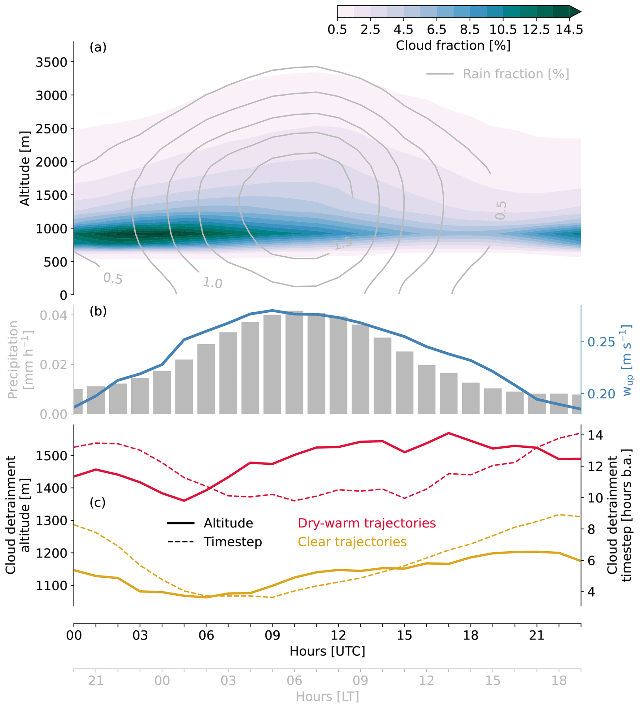
Figure 5 Diel cycle of (a) cloud (filled contours) and rain (contours) fraction at different levels, defined as fraction of grid points per model level exceeding the threshold of 10 and 1 mg kg⁻¹ cloud and rain water, respectively; (b, left) average precipitation; (b, right) strength of updraughts at cloud base, defined as the mean of positive vertical velocities in cloud grid points (w_up); and (c) median cloud detrainment altitude (continuous; left y axis) and time step (as hour before arrival; dashed; right y axis) of the air parcels arriving at clear (yellow) and dry-warm (red) cloud base grid points, only considering those air parcel trajectories that have been inside a cloud (Sect. 2.4). The hour-of-the-day mean values in the domain 54.5–61^∘ W and 11–16^∘ N during the period 20 January to 13 February 2020 are shown. Data: (a, b) COSMO_iso,1 km and (c) COSMO_iso,5 km trajectories.

Assuming an approximately closed cloud-relative circulation, we expect that the variation of the ascending branch (i.e. updraught strengths, rain rates, cloud fraction, and vertical extent) over the day triggers a response in the descending branch. A physically meaningful response can be found in the COSMO_iso,5 km trajectories: air parcels arriving at dry-warm cloud base grid points require 10–14 h to cover the distance from the altitude where they were detrained from a cloud to the altitude of cloud base (red dashed line in Fig. 5c). In other words, the altitude at which these air parcels were detrained (red continuous line in Fig. 5c) should reflect the cloud characteristics 10–14 h earlier. If we, for example, look at the air parcels arriving 13:00 LT (17:00 UTC) at dry-warm cloud base grid points, we learn that these air parcels were detrained 12 h earlier (the time of the day with the highest low-level cloud fraction; Fig. 5a) from clouds at 1570 m. Contrastingly, the air parcels arriving 01:00 LT (05:00 UTC) at dry-warm cloud base grid points were detrained 11 h earlier (the time of the day with the lowest low-level cloud fraction; Fig. 5a) from clouds at 1360 m. Thus, the amount of low-level clouds and their vertical extent determines the average detrainment altitude of dry-warm air parcels.

A similar diel cycle is found for the air parcels arriving at clear grid points at cloud base. However, the subsidence times are shorter (4–9 h; yellow dashed in Fig. 5c), and the cloud detrainment altitudes are correspondingly lower (1060–1200 m; yellow continuous in Fig. 5c). Earlier (Sect. 2.3), we formulated the hypothesis that the dry-warm and clear cloud base characteristics emerge due to different processes. The trajectory analysis discussed here suggests that it is more accurate to speak of different paths than processes. The air forming the dry-warm patches originates from altitudes where it is likely also mixed with air from the free troposphere. Contrastingly, the clear environments form out of air that was detrained from clouds earlier, at lower altitudes. In our understanding, both categories belong to the subsiding branch of the cloud-relative circulation, with the dry-warm path connecting cloud base with higher detrainment altitudes.

If we link the two different transport histories with the idealised schematic, illustrating processes altering δ²H (Fig. 1a), we come to the conclusion that we must find contrasting isotope signals in the three cloud base environments dry-warm, clear, and cloud. The dry-warm air has ascended the furthest and should therefore be the most depleted environment. In addition, mixing with free tropospheric air would further deplete the vapour before it subsides into the dry-warm patches at cloud base. The clear air has ascended less and should therefore be more enriched. In the cloud air, condensation and rainout of heavy isotopes just started, and therefore its vapour should be the most enriched.

The above considerations are confirmed by the data. Looking at δ²H (Fig. 6, left y axis), we find the most enriched vapour in the cloud and the most depleted vapour in the dry-warm cloud base environments. Similar characteristics are found for q (Fig. 6, right y axis), with the highest values in the cloud and the lowest in the dry-warm environments (as expected from the definition of dry-warm). The three environments differ not only in absolute values but also in the diel cycles. The diel cycles of δ²H and q are more pronounced for the dry-warm (amplitudes of ∼4 ‰ and 1.6 g kg⁻¹) and clear environments (amplitudes of ∼1.6 ‰ and 0.8 g kg⁻¹) than for the cloud environments (amplitudes of ∼0.9 ‰ and 0.5 g kg⁻¹). The cloud patches are fed by updraughts bringing moisture from the subcloud layer, in which the amplitude of the variability in q and δ²H is small and of about the same extent as observed in clouds (see part 1 of this study and Appendix A). While the cloudy grid points are thus largely unaffected by the diel cycle of convection, the dry-warm and clear grid points reach their most depleted and driest state shortly after noon local time, when cloud base cloudiness is minimal (Fig. 5a), updraughts are weak (Fig. 5b) and air parcels from comparably high altitudes arrive in the two cloud base environments (Fig. 5c).

g

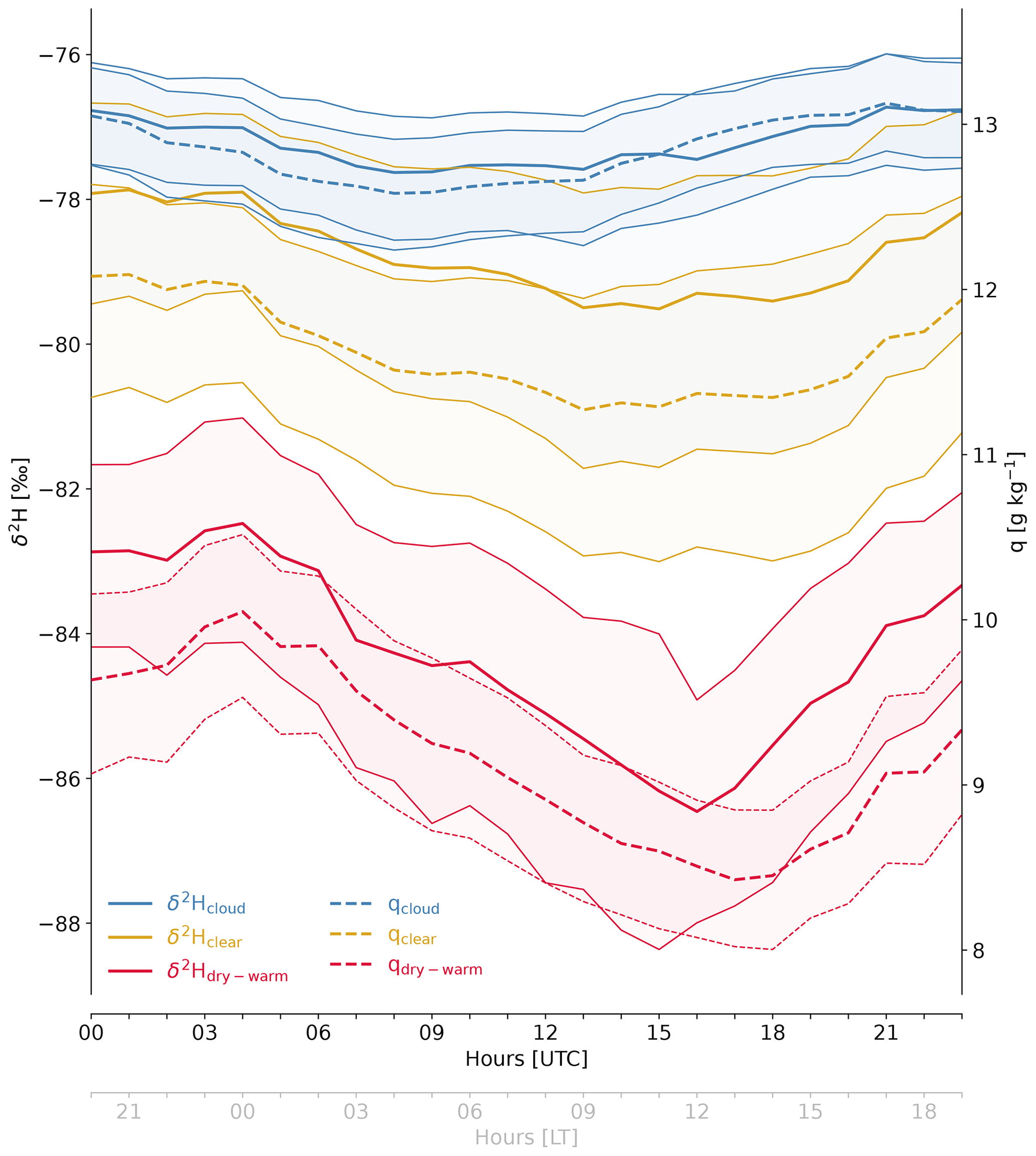
Figure 6 Diel cycle of δ²H in vapour with the median shown as a thick line and the 25–75-percentile range as shading/thin lines (continuous; left y axis) and q (dashed; right y axis) of cloud (blue), clear (yellow), and dry-warm (red) cloud base grid points. The hour-of-the-day mean values in the domain 54.5–61^∘ W and 11–16^∘ N during the period 20 January to 13 February 2020 are shown. Data: COSMO_iso,1 km.

Two mechanisms likely contribute to the drying and depletion of the clear and dry-warm cloud base grid points over the course of the day: (1) a small immediate effect due to the decrease in cloud fraction, which reduces the moistening and enrichment of the clear and dry-warm patches through lateral detrainment from surrounding clouds, and (2) a dominating temporally delayed effect due to the vertical growth of clouds, which has the consequence that the detrainment from clouds happens at increasing altitudes where temperature is lower and, therefore, saturated q is less. With increasing altitudes, the isotope signal is also more depleted due to the continuous condensation and rainout in the convective updraughts which transport the vapour to these altitudes in the first place. Assuming that the vapour detrained from clouds experiences little to no phase changes or mixing with advected vapour during its journey back to cloud base (i.e. closed circulation), it follows that its isotope signal is approximatively conserved. Thus, the higher the detrainment from clouds, the lower the amount of vapour that returns to cloud base and the more depleted its isotope signal. This mechanism would explain the differences of q and δ²H between the clear and dry-warm patches, as well as their diel cycles. A link between the altitude of origin (cf. detrainment altitude) and the depletion of the vapour was previously determined by Risi et al. (2019). Furthermore, George et al. (2023) discovered that the ascending branch of mesoscale circulations is associated with a moisture accumulation in the subcloud layer and at cloud base, while the descending branch is associated with a moisture deficit. Both studies back our suggestion that the mesoscale spatial and temporal variability of cloud base isotopes is closely linked to the cloud-relative circulation.

As mentioned at the beginning of this section, we have to be careful with the absolute values of the variables derived from the COSMO_iso,5 km trajectories when combining them with variables from the COSMO_iso,1 km simulation. A comparison to literature, however, gives confidence that the obtained values for the detrainment time and altitude are meaningful. George et al. (2023) identified shallow mesoscale circulations in EUREC⁴A dropsonde observations as dipoles between the divergence in the subcloud layer and the divergence in the cloud layer. They find the highest lagged anti-correlation between the divergences of the two layers for a temporal lag of 7 to 8 h, which can be interpreted as a minimal lifetime of these circulations. This observation supports the subsidence times of 4 to 14 h as identified with our COSMO_iso,5 km trajectories. Furthermore, their definition of the cloud layer, ranging from 900 to 1500 m, largely overlaps with our diagnosed detrainment altitudes, giving them additional independent credibility.

In this section, we showed that at the subdaily timescale, q or δ²H at cloud base vary little inside clouds, while their variations in the clear and dry-warm environments reflect the deepening of convection over the day, which (with a 4–9 h and a 10–14 h lag, respectively) causes drying and vapour depletion of the clear and dry-warm environments. The information gained from q and δ²H seems congruent, while the d-excess contains no signal of a diel cycle in any cloud base environment (not shown; Villiger, 2022), pointing towards a dominant control by the large-scale circulation (see Sect. 4). Finally, we found evidence for the fact that the circulation associated with clouds is only a few hundred metres deep.

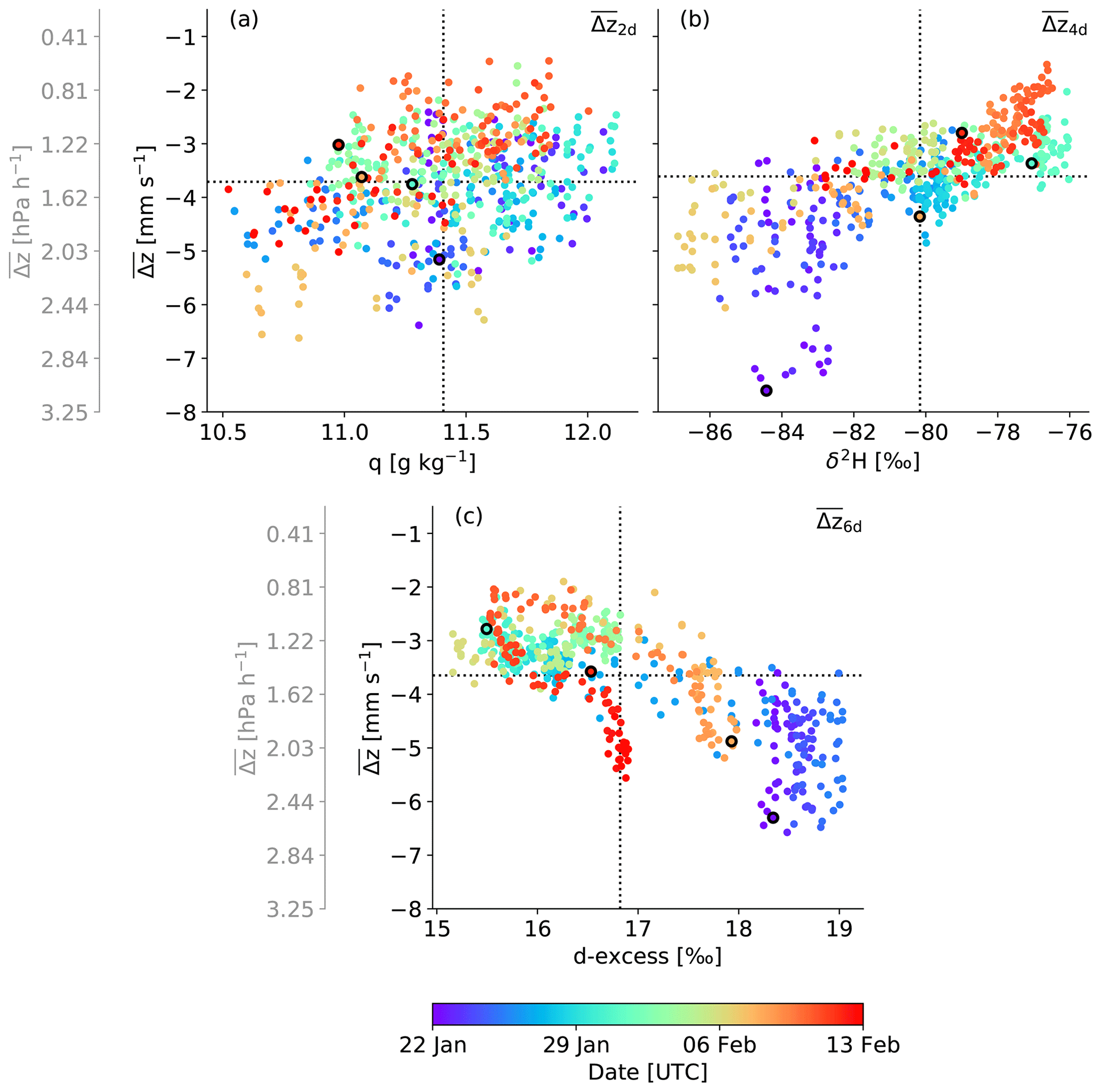
Figure 7 Relation between vapour (a) q, (b) δ²H, and (c) d-excess of the COSMO_iso,10 km air parcels at their arrival near cloud base and their mean vertical displacement (${\stackrel{\mathrm{‾}}{\mathrm{\Delta }z}}_{X\mathrm{d}}$) over the period (X d), which yielded the highest correlation (Table 1), i.e. 2, 4, and 6 d. The data points are coloured according to the arrival time step of the air parcels. Shown are the mean values over the 138 COSMO_iso,10 km air parcels arriving simultaneously (every hour from 22 January to 13 February 2020) at the three cloud base trajectory starting levels (940, 920, and 900 hPa) in the domain 54.5–61^∘ W and 11–16^∘ N. See Sect. 2.5 for details about how the subsidence is calculated. The dashed black lines indicate the mean values of the respective x and y variable over all arrival time steps. The data points with black borders represent arrival at 12:00 UTC on 22 January 2020, 15:00 UTC on 31 January 2020, 18:00 UTC on 8 February 2020, and 18:00 UTC on 12 February 2020. Data: COSMO_iso,10 km.

4 Cloud base isotopes and the large-scale circulation

This section investigates which of the three variables, q, δ²H, or d-excess, at the base of trade-wind clouds is most strongly influenced by the large-scale circulation. For this, we use trajectories calculated based on the COSMO_iso,10 km simulation (Sect. 2.5), which arrive evenly distributed near cloud base and are not targeted at cloud, clear, or dry-warm environments. We use the mean vertical displacement over time periods exceeding 1 d (${\stackrel{\mathrm{‾}}{\mathrm{\Delta }z}}_{X\mathrm{d}}$) to distinguish between large-scale circulation patterns. For Hadley-cell-like subsidence, resulting from the balance between radiative cooling and adiabatic warming, a vertical displacement of ∼1.5 hPa h⁻¹ (Salathé and Hartmann, 1997) is expected. For air parcels that go through an extratropical dry intrusion before arriving in the trades (Aemisegger et al., 2021; Villiger et al., 2022), the subsidence of individual air parcels exceeds ∼8 hPa h⁻¹ (Raveh-Rubin, 2017).

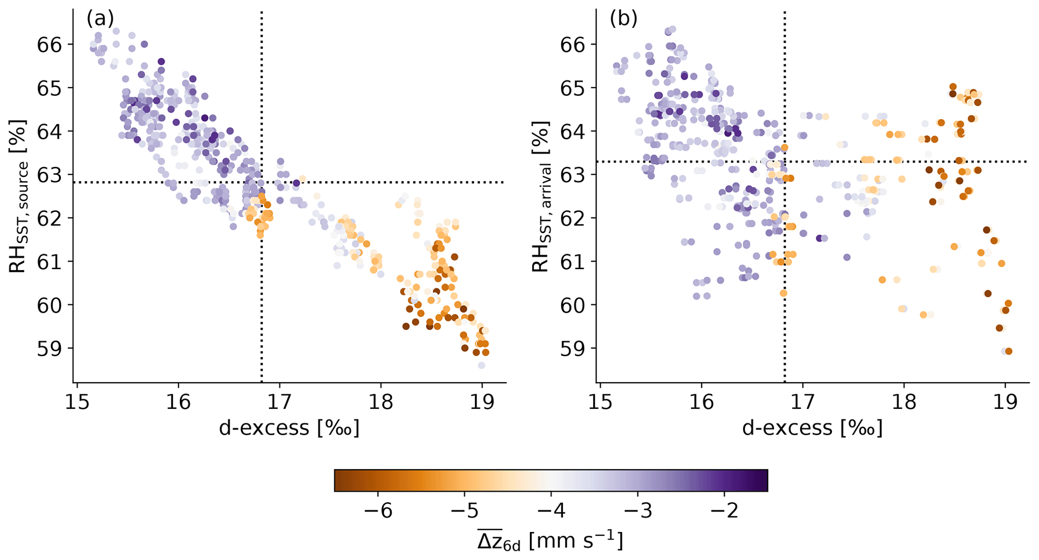
Figure 8 Relation between relative humidity with respect to sea surface temperature (RH_SST) and d-excess in vapour of the COSMO_iso,10 km air parcels at their arrival near cloud base. (a) RH_SST at the moisture source of the air parcels (Pearson correlation coefficient = −0.92; two-tailed p value $<{\mathrm{10}}^{-\mathrm{6}}$); (b) RH_SST at the air parcel's arrival location (Pearson correlation coefficient = −0.37; two-tailed p value < 10⁻⁶). The data points are coloured according to the mean vertical displacement of air parcels during the last 6 d before arrival at cloud base (${\stackrel{\mathrm{‾}}{\mathrm{\Delta }z}}_{\mathrm{6}\mathrm{d}}$, i.e. the variable shown on the y axis of Fig. 7c). Shown are the mean values over the 138 COSMO_iso,10 km air parcels arriving simultaneously (from 22 January to 13 February 2020) at the three cloud base trajectory arrival levels (940, 920, and 900 hPa) in the domain 54.5–61^∘ W and 11–16^∘ N. The dashed black lines indicate the mean values of the respective x and y variable over all arrival time steps. Data: COSMO_iso,10 km.

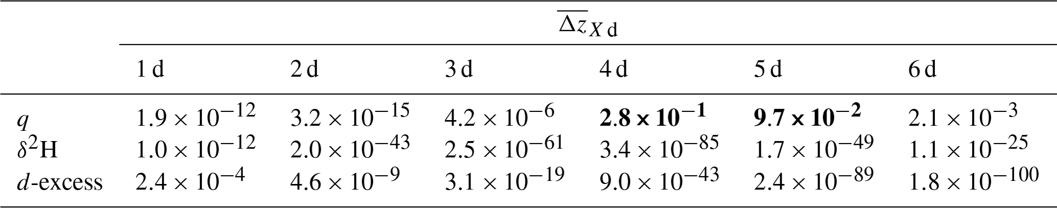
The strongest link between the large-scale circulation and the cloud base δ²H in the trades is found if the air parcel's vertical displacement during 4 d before arrival is considered (Table 1). For the d-excess, the strongest link is found for 6 d or more (the trajectory length is limited by the domain size in this analysis). The correlations are weaker for shorter or longer timescales, and the relationship is such that the vapour is more depleted and has a higher d-excess when the subsidence of the air parcels is stronger (Fig. 7b, c). In comparison to the isotope variables, q is less influenced by the large-scale vertical displacement (comparably low correlations, with the maximum found for 2 d; Table 1 and Fig. 7a), illustrating the limited memory of moist processes registered by q alone. This difference in memory of the history of moist processes along the flow in q and δ²H is due to the fact that q alone is determined to first order by the temperature just before the detrainment from clouds (i.e. last saturation paradigm; see Sherwood, 1996; Sherwood et al., 2010), while the δ²H contains information on both [¹H₂¹⁶O] and [¹H²H¹⁶O], which relates to the condensation history in the clouds. The d-excess in turn connects to the non-equilibrium conditions at the evaporative moisture source, while being at first order unaffected by equilibrium cloud processing.

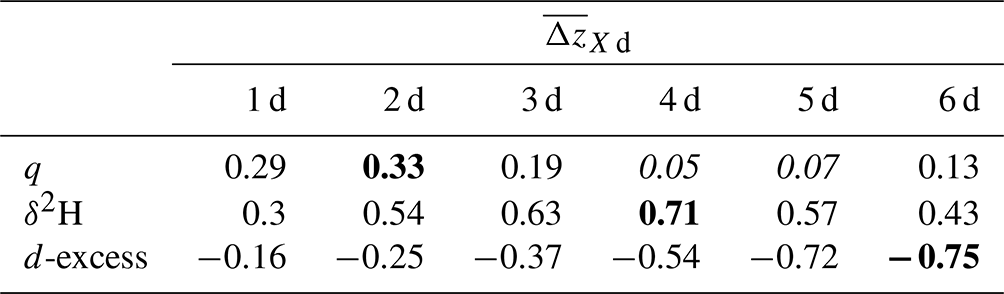
Table 1 Pearson correlation coefficients between vapour q, δ²H, and d-excess of the COSMO_iso,10 km air parcels at their arrival near cloud base and their mean vertical displacement (${\stackrel{\mathrm{‾}}{\mathrm{\Delta }z}}_{X\mathrm{d}}$; Sect. 2.5) during the X=1…6 d before arrival. The correlations are calculated between the mean values of the 138 air parcels arriving every hour between 22 January and 13 February 2020 (shown in Fig. 7). The strongest correlation for each variable is shown in bold. Combinations with no statistically significant association between the two variables (i.e. two-tailed p value >0.05; see p values in Table B1) are highlighted in italics. Data: COSMO_iso,10 km.

The physical link between the subsidence and δ²H is straightforward: the stronger the subsidence, the isotopically lighter the vapour because it originates from higher altitudes (Risi et al., 2019). The link between the subsidence and the d-excess can be explained by the contrasting conditions at the site where the vapour is evaporated and picked up by the air parcels embedded in the large-scale circulation (i.e. at the moisture source; see examples in Appendix C). Air parcels descending within an extratropical dry intrusion are expected to be drier and to create a stronger near-surface humidity gradient (i.e. lower RH_SST) at the moisture source (increasing the d-excess) than air parcels crossing the North Atlantic at low levels within the comparably moist trade winds where frequent detrainment of cloudy air occurs (lowering the d-excess; Fig. 1b). This interplay between large-scale subsidence, humidity gradient, and d-excess is visualised in Fig. 8. The air parcel's d-excess at arrival is clearly more strongly influenced by the humidity gradient at the moisture source (Fig. 8a) than by the humidity gradient at the arrival location (Fig. 8b).

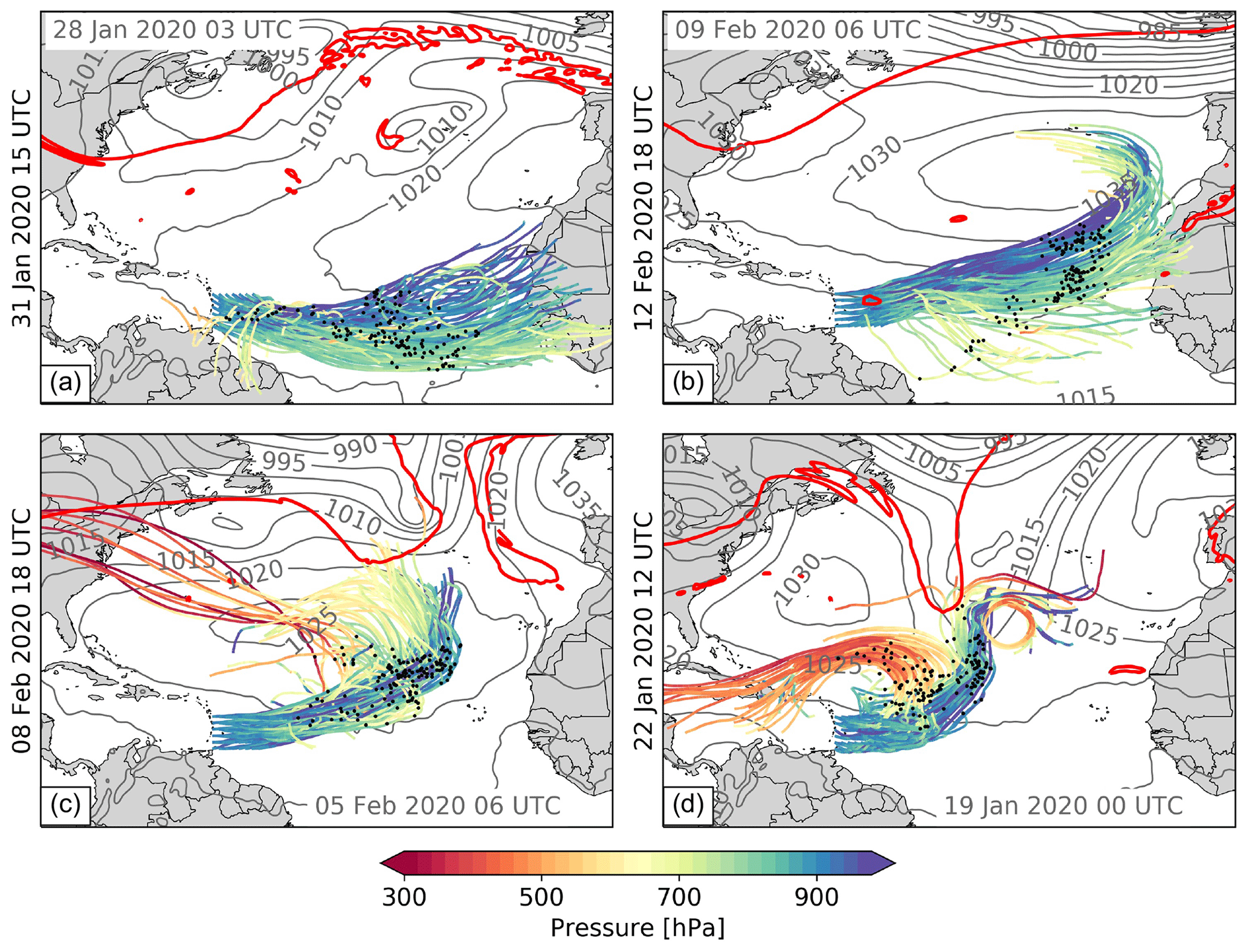
Figure 9 COSMO_iso,10 km trajectories for exemplary dates with different strength of the large-scale 6 d subsidence (the corresponding moisture sources are shown in Fig. C1). Arrival time steps are indicated in black on the left side of the panels. The dates were selected from Fig. 7 as indicated by the black bordered markers. The trajectories arrive at 940, 920, and 900 hPa in the domain 54.5–61^∘ W and 11–16^∘ N. Together with each air parcel's position (black dots) 3.5 d before arrival, the sea level pressure (grey contours) and the dynamical tropopause (2 pvu at 320 K; red contours) are shown for the corresponding date indicated in grey at the top left or bottom right of each panel. Shown are the domain 0–85^∘ W and 5^∘ S–55^∘ N and the air parcels arriving (a) at 15:00 UTC on 31 January (q=11.3 g kg⁻¹, δ²H $=-\mathrm{77.1}$ ‰, d=15.5 ‰, 6 d subsidence $=-\mathrm{2.8}$ mm s⁻¹ or 1.1 hPa h⁻¹); (b) at 18:00 UTC on 12 February (q=11.0 g kg⁻¹, δ²H $=-\mathrm{79.0}$ ‰, d=16.5 ‰, 6 d subsidence $=-\mathrm{3.6}$ mm s⁻¹ or 1.5 hPa h⁻¹), (c) at 18:00 UTC on 8 February (q=11.1 g kg⁻¹, δ²H $=-\mathrm{80.2}$ ‰, d=17.9 ‰, 6 d subsidence $=-\mathrm{4.9}$ mm s⁻¹ or 2 hPa h⁻¹), and (d) at 12:00 UTC on 22 January 2020 (q=11.4 g kg⁻¹, δ²H = −84.4 ‰, d=18.3 ‰, 6 d subsidence = −6.3 mm s⁻¹ or 2.6 hPa h⁻¹). The dates are sorted according to the strength of the subsidence over 6 d, starting with the case with the weakest subsidence in panel (a). Data: COSMO_iso,10 km.

The maximum correlation shown in Table 1 is slightly higher for the d-excess than for the δ²H and small for q. Moreover, the vertical displacement time window leading to the highest correlation extends further back for the d-excess than for δ²H or humidity. Both findings suggest that of the three variables, the d-excess is most strongly influenced by the large-scale circulation through the conditions created at the moisture source. This meets expectations, as the d-excess is known to be sensitive to the non-equilibrium fractionation conditions at the moisture source (Pfahl and Wernli, 2008; Aemisegger et al., 2021) and less to subsequent cloud processes, which often happen under conditions close to equilibrium. Contrastingly, δ²H is sensitive to equilibrium and non-equilibrium processes, meaning the source signal is more quickly overwritten than the one of d-excess.

The mean vertical displacement over all arrival time steps is 1.5 hPa h⁻¹ (Fig. 7), which corresponds to a Hadley-cell-like descent. However, it can be substantially stronger or weaker for individual time steps. To illustrate the variability in the large-scale circulation, four time steps with contrasting 6 d subsidence are selected (Fig. 9). The two cases with weaker subsidence (Fig. 9a, b) are associated with the typical zonal flow of the trades. In the two cases with stronger subsidence (Fig. 9c, d), the trades are interrupted by Rossby-wave breaking events over the central North Atlantic, which steer the air parcels from the extratropics towards low latitudes and cause a rapid descent along the slanted isentropes from the upper into the lower troposphere. As expected from the correlation analysis above (Table 1, Fig. 7), the different large-scale circulation patterns of the four cases lead to clear differences in the d-excess (ranging from 15.5 ‰ to 18.3 ‰) and the δ²H (ranging from −77.1 ‰ to −84.2 ‰) at the air parcel's arrival location but not in q (ranging from 11.0 to 11.4 g kg⁻¹). This analysis on the influence of the large-scale circulation on cloud base isotopes showed, that on a daily timescale the d-excess is mainly impacted by the different regimes of the large-scale flow in the winter trades, while δ²H connects to the strength of the large-scale subsidence in addition to the strong influence of the cloud-relative circulation.

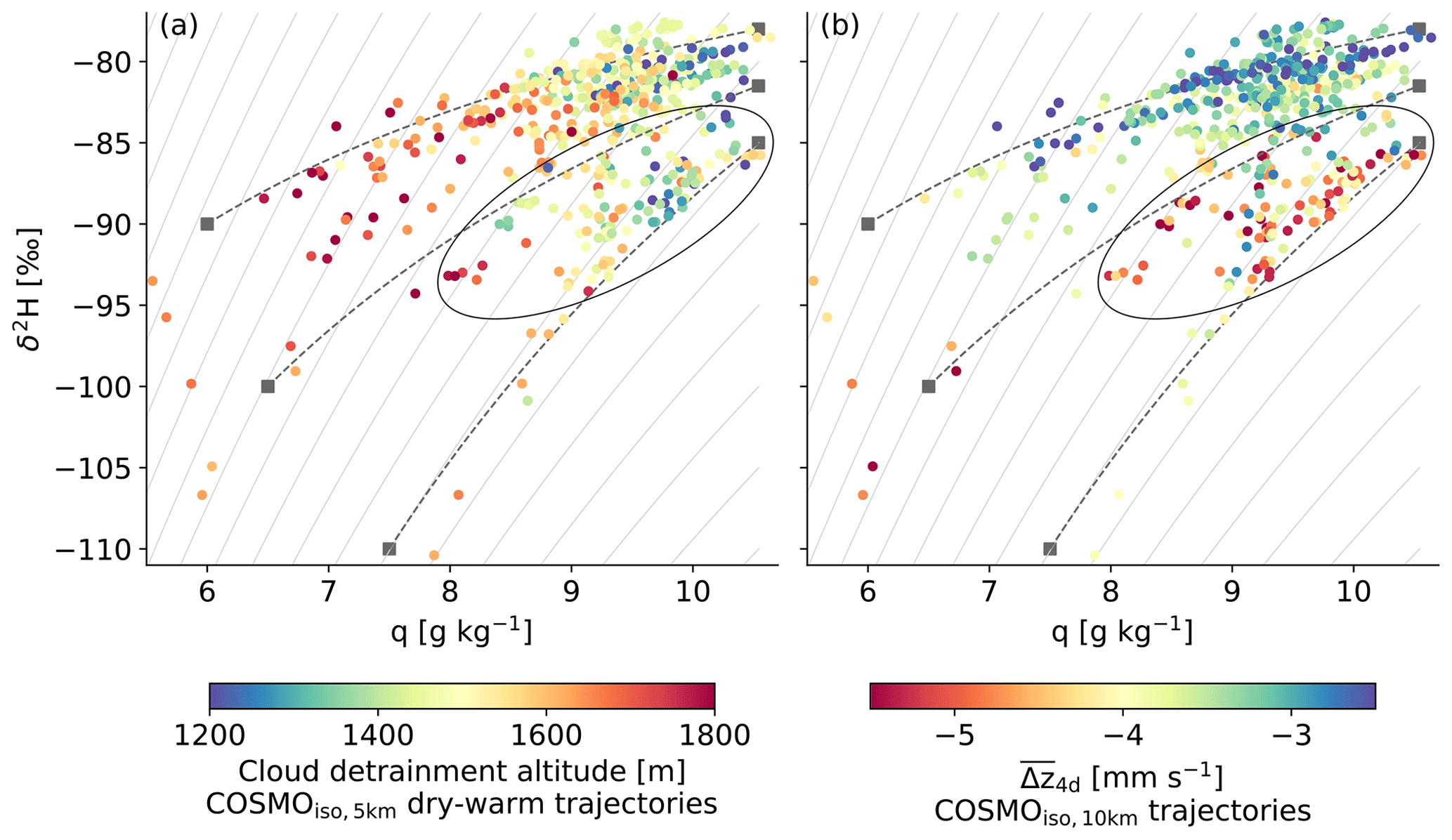
Figure 10 Relation between hourly median values of q and δ²H in the vapour of the cloud base grid points identified as dry-warm in the domain 54.5–61^∘ W and 11–16^∘ N from COSMO_iso,1 km. They are coloured according to (a) the cloud detrainment altitude derived from the COSMO_iso,5 km trajectories and (b) $\stackrel{\mathrm{‾}}{\mathrm{\Delta }z}$ over 4 d from the COSMO_iso,10 km trajectories. Rayleigh distillation curves for an open system (i.e. assuming 100 % precipitation efficiency; light grey continuous) and three exemplary mixing lines (dark grey dashed) with the mixing endmembers (dark grey squares) are shown for reference. Data points with enhanced large-scale subsidence leading to low δ²H values are encircled in black.

5 Summary and conclusion

In this final section, we combine the insights from relating isotope signals at cloud base to the circulation at different scales. In a first step (Sect. 3), we analysed the imprint of the cloud-relative circulation on cloud base water vapour isotopes in the trade-wind region. For this, we distinguished between three cloud base environments, i.e. cloud, clear, and dry-warm. We showed that the three environments differ regarding the values and diel cycles of q and δ²H, and we could attribute these differences to distinct processes in the cloud-relative circulation (see underlying concept in Fig. 1a). Furthermore, we demonstrated that q and δ²H of the cloud environment remain largely unaffected by the vertical growth of convection over the day, while the other two environments show a diel cycle linked to the cloud fraction at the cloud base and the cloud depth. Through the vertical growth of the clouds during the day, the altitude at which the vapour is detrained from the cloud is lifted. This cloud detrainment altitude of the air parcels arriving in the clear or dry-warm patches was identified as the main control of the degree of drying and depletion at cloud base. Since the cloud detrainment altitudes are higher for the dry-warm than for the clear environment, the drying and depletion is stronger in the former. The information gained from q and δ²H was largely congruent. However, by combining the two variables for the dry-warm environment (Fig. 10a), we find a group of data points (encircled in black) that is shifted towards lower δ²H but shows no peculiarities in q or the detrainment altitude. The stronger depletion of these data points can only be understood if the influence of the large-scale circulation is taken into account.

We investigated the imprint of the large-scale circulation on cloud base water vapour isotopes in a second step (Sect. 4). We illustrated that δ²H and d-excess of the vapour near the cloud base (independently of the cloud base environment, i.e. cloud, clear, or dry-warm), but not q, vary on the synoptic scale following changes in the large-scale circulation in a physically meaningful way. Namely, the vapour in the trade-wind region is more depleted and has a higher d-excess the stronger the subsidence (i.e. the more negative the vertical displacement) during the preceding 4 to 6 d. The δ²H in cloud base vapour was found to be most strongly linked to the 4 d vertical displacement (Pearson correlation of 0.71), which also explains the more depleted data points (encircled in black) in Fig. 10. Contrastingly, the d-excess is most strongly linked to the 6 d vertical displacement (Pearson correlation of −0.75). The strong link between the d-excess and the large-scale circulation found here is in agreement with Aemisegger et al. (2021, their Fig. 16), who found a clear link (Pearson correlation of −0.73) between the d-excess in vapour measured on Barbados in the subcloud layer and the distance to the moisture source, during a field experiment in early 2018. The analysis also showed that the identified pathways of air parcels arriving in the lower troposphere qualitatively agree with the ones identified in Villiger et al. (2022).

In Fig. 10, we summarise the main findings of this study. Namely, the values of q and δ²H in dry-warm cloud base environments are determined (a) by the cloud-relative circulation through the cloud detrainment altitude (reflecting the diel cycle of convection) as well as (b) by the large-scale subsidence reflecting different circulation patterns with distinct moisture source conditions. The isotope-shaping processes within these two circulations occur at different timescales. While the cloud detrainment takes place 4 to 14 h before the air parcels arrive at cloud base, the moisture source conditions are shaped by the subsidence during the 4 to 6 d before the air parcels arrive in the trades. We, here, focus on the dry-warm environments because it is the cloud base environment where the influence from the cloud-relative circulation is strongest.

To deepen our understanding of the hydrological cycle associated with shallow trade-wind cumulus clouds, the role of mixing and liquid-vapour interaction processes embedded in the cloud-relative circulation should be examined in more detail. In Fig. 10 the δ²H–q value pairs of dry-warm cloud base environments together with reference lines illustrating the impact of mixing (dark grey dashed lines) and precipitation production in clouds (assuming 100 % precipitation efficiency; light grey lines) show that a combination of processes is involved including mixing and microphysical processes. To disentangle the influence of these processes on the isotope signal, the cloudy profiles from EUREC⁴A observations and simulations should be studied in more detail in the future. Furthermore, a tagging experiment with numerical tracers distinguishing subcloud layer and free-tropospheric moisture would help to disentangle the contribution of the circulations associated with clouds of varying depths and the large-scale circulation (Brient et al., 2019). Our analysis demonstrated that isotopes represent the integral signal of past moist atmospheric processes encountered along the flow. Particularly novel was the finding that isotopes serve as indicators for changes in atmospheric circulations on various scales. By investigating the isotope signal at cloud base in the trade-wind region, we could identify the imprint of different large-scale circulation patterns and the circulation associated with clouds that, in concert, determine the formation of clouds and precipitation.

Appendix A: Evaluation of the simulated diel cycle with observations

In this appendix, the modelled diel cycles (Fig. A2) of near-surface humidity and isotope variables are evaluated using observations (Bailey et al., 2023) from the EUREC⁴A field campaign (Stevens et al., 2021). For this purpose, the data points from the lowest model level and the grid point closest to the Barbados Cloud Observatory (BCO; Fig. A1) were extracted from the three COSMO_iso simulations. Note that an evaluation of the diel cycles of cloud base variables is not possible because no continuous measurements at this altitude exist. Cloud base measurements from the ATR42 were all collected between 03:00 and 18:00 LT.

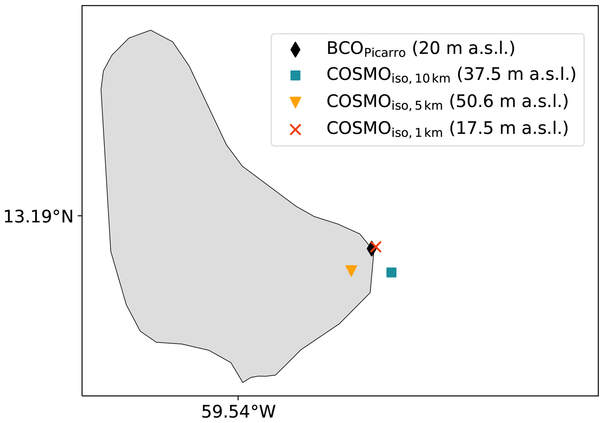
Figure A1 Grid point of the COSMO_iso,10 km (teal), COSMO_iso,5 km (yellow), and COSMO_iso,1 km (red) model set-up closest to the BCO (black marker). The altitude of the lowest model level is given in brackets (in metres above sea level ($\mathrm{m}\mathrm{a}.\mathrm{s}.\mathrm{l}.$)). The BCO is located 17 $\mathrm{m}\mathrm{a}.\mathrm{s}.\mathrm{l}.$ (Stevens et al., 2016, their Fig. 2), and the isotope observations were conducted at ∼3 m above ground (Bailey et al., 2023).

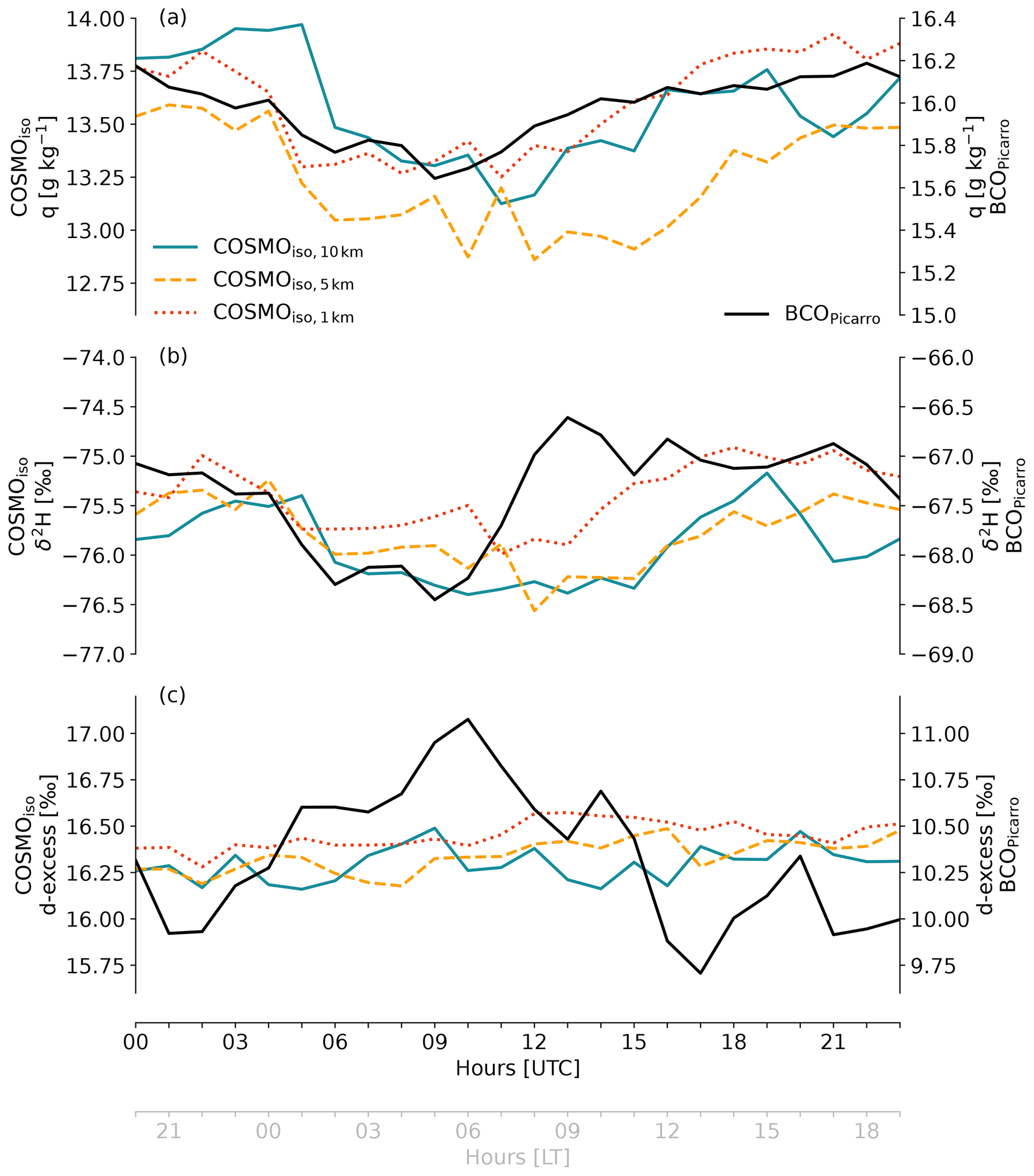
Figure A2 Diel cycles of near-surface (a) q, (b) δ²H, and (c) d-excess in the COSMO_iso,10 km (teal), COSMO_iso,5 km (yellow dashed), and COSMO_iso,1 km (red dotted) simulations together with observations collected during EUREC⁴A at the Barbados Cloud Observatory (BCO; black, labelled BCO_Picarro; see Bailey et al., 2023, for a description of the BCO observations). For all four data sets, the period from 20 January to 13 February 2020 is considered for the calculation of the diel cycle. For COSMO_iso, the data from the lowest model level and the grid point closest to the BCO are selected (Fig. A1). Note that the lowest model level is different for the three COSMO_iso set-ups and does not correspond to the altitude of the observations. Therefore, different y axes are used for the simulations (left) and the observations (right).

Appendix B: Relation between cloud base conditions and large-scale circulation

In this appendix, two-sided p values (Table B1) for the correlations listed in Table 1 are given. They indicate that all correlations are statistically significant, except for the one between cloud base q and the large-scale subsidence over 4 d (${\stackrel{\mathrm{‾}}{\mathrm{\Delta }z}}_{\mathrm{4}\mathrm{d}}$) or 5 d (${\stackrel{\mathrm{‾}}{\mathrm{\Delta }z}}_{\text{5d}}$; see Table B1).

Table B1 Two-sided p values indicating whether there is a statistically significant association between two variables. The same variable combinations as in Table 1 are investigated. Non-significant associations between two variables (i.e. two-tailed p value >0.05) are highlighted in bold. Data: COSMO_iso,10 km.

Appendix C: Moisture uptake along the COSMO_iso,10 km trajectories

In this appendix, the moisture uptakes along the trajectories shown in Fig. 9 are displayed (i.e. the moisture sources).

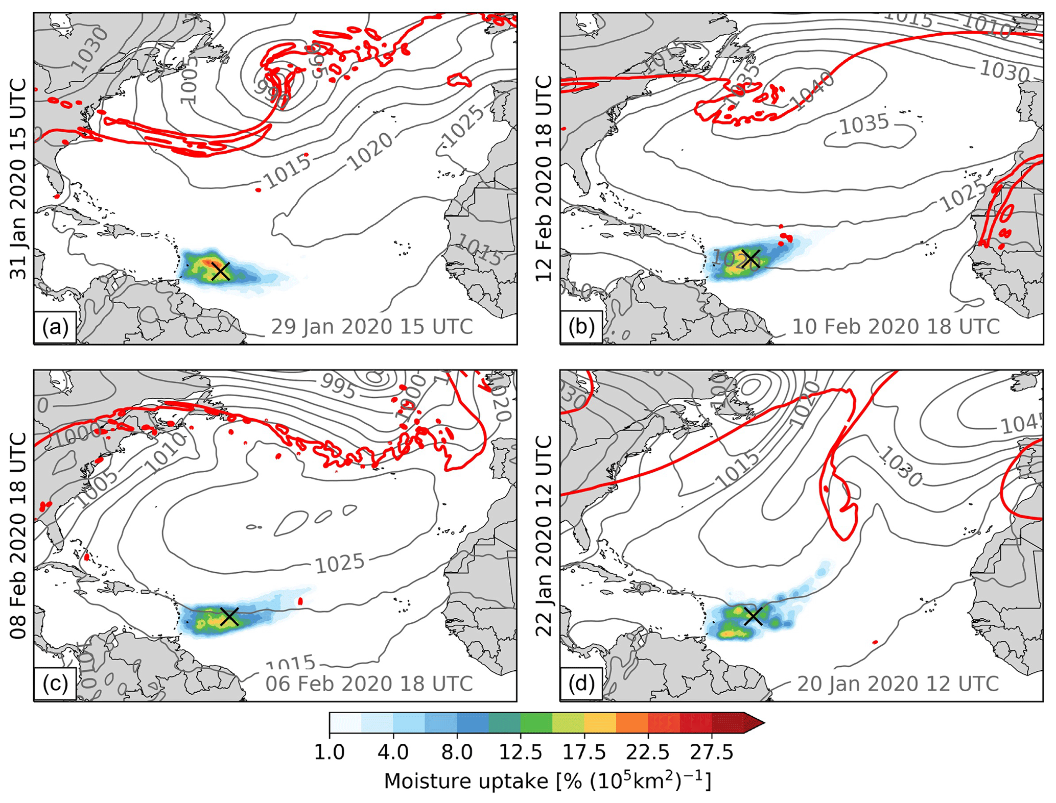
Figure C1 COSMO_iso,10 km moisture sources for the trajectories shown in Fig. 9. The arrival time steps, indicated in black on the left side of the panels, are (a) 15:00 UTC on 31 January, (b) 18:00 UTC on 12 February, (c) 18:00 UTC on 8 February, and (d) 12:00 UTC on 22 January 2020. The sea level pressure (grey contours) and the dynamical tropopause (2 pvu at 320 K; red contours) are shown 2 d before arrival. The corresponding date is indicated in grey at the bottom right of each panel. Shown is the domain 0–85^∘ W and 5^∘ S–55^∘ N. Data: COSMO_iso,10 km.