Relations between cyclones and ozone changes in the Arctic using data from satellite instruments and the MOSAiC ship campaign

Large-scale meteorological events (e.g. cyclones), referred to as synoptic events, strongly influence weather predictability but still cannot be fully characterised in the Arctic region because of the sparse coverage of measurements. Due to the fact that atmospheric dynamics in the lower stratosphere and troposphere influence the ozone field, one approach to analyse these events further is the use of space-borne measurements of ozone vertical distributions and total columns in addition to conventional parameters such as pressure or wind speed. In this study we investigate the link between cyclones and changes in stratospheric ozone by using a combination of unique measurements during the Multidisciplinary drifting Observatory for the Study of Arctic Climate (MOSAiC) ship expedition, ozone profile and total column observations by satellite instruments (OMPS-LP, TROPOMI), and ERA5 reanalysis data. The final goal of the study is to assess whether the satellite ozone data can be used to obtain information about cyclones and provide herewith an additional value in the assimilation by numerical weather prediction models. Three special cases during the MOSAiC expedition were selected and classified for the analysis. They are one “normal” cyclone, where a low surface pressure coincides with a minimum in tropopause height, and two “untypical” cyclones, where this is not observed. The influence of cyclone events on ozone in the upper-troposphere lower-stratosphere (UTLS) region was investigated, using the fact that both are correlated with tropopause height changes. The negative correlation between tropopause height from ERA5 and ozone columns was investigated in the Arctic region for the 3-month period from June to August 2020. This was done using total ozone columns and sub-columns from TROPOMI, OMPS-LP, and MOSAiC ozonesonde data. The greatest influence of tropopause height changes on ozone contour levels occurs at an altitude between 10 and 20 km. Moreover, the lowering of the 250 ppb ozonopause (at about 11 km altitude) below 9 km was used to detect cyclones using OMPS-LP ozone observations. The potential of this approach was demonstrated in two case studies where the boundaries of cyclones could be determined using ozone observations. The results of this study can help improve our understanding of the relationship between cyclones, tropopause height, and ozone in the Arctic and demonstrate the usability of satellite ozone data in addition to the conventional parameters for investigating cyclones in the Arctic.

1 Introduction

The Arctic is a region that is particularly sensitive to climate change and has experienced dramatic changes in recent decades (Stroeve and Notz, 2018; Box et al., 2019). More frequent and intense synoptic events, such as cyclones, are one effect of climate change in the Arctic (e.g. Rinke et al., 2017; Day et al., 2018; Zhang et al., 2023). These events not only affect local weather conditions but also generate preferred patterns of seasonal circulation in the Arctic and can contribute to monthly to seasonal large-scale circulation patterns (Wernli and Papritz, 2018; Graversen and Burtu, 2016). Measuring and monitoring synoptic events in the Arctic is therefore of great importance to gain a better understanding of the role of the Arctic in the global climate. Sea level pressure, air temperature, wind speed and direction, and total column water vapour are primarily used as atmospheric parameters to characterise such events (Rinke et al., 2021). Another important parameter is ozone, which is a dynamic tracer of troposphere–stratosphere interactions. Since cyclones exert a large influence in this altitude region, ozone is affected by them (Millán and Manney, 2017). Because the Arctic is a remote and difficult-to-access region, it is challenging to make accurate and comprehensive measurements. Existing observing stations are limited and the coverage of measurements is often inadequate (Curry et al., 2004). Ozone satellite data provide additional information to study changes in the Arctic induced by synoptic events because they offer wide coverage and continuous observations that go beyond the limited measurements available on land and at sea (Veefkind et al., 2012; Flynn et al., 2014).

Synoptic-event-induced ozone changes were first investigated by Dobson et al. (1929), who studied the connection between weather events and their influence on the total ozone column. Not long after, Meethan and Dobson (1937) showed a significant correlation between the total ozone column and the tropopause height. This is explained by the fact that a downward movement of the air masses causes an increase in the total ozone column because the ozone is sucked into the column, and an upward movement causes a reduction in the total ozone column because the ozone is pushed out of the column (Reed, 1950; Barsby and Diab, 1995; Zou and Wu, 2005). This negative correlation between tropopause height and ozone columns (e.g. Appenzeller et al., 2000; Steinbrecht et al., 1998, 2001) enables us to investigate weather phenomena that influence atmospheric dynamics using ozone data (Zou and Wu, 2005). For example, Orsolini et al. (1998) identified storm tracks during winter and spring by analysing daily gridded Total Ozone Mapping Spectrometer (TOMS) ozone data. Davis et al. (1999) developed a method for determining three-dimensional winds from TOMS ozone data. Using high-resolution mesoscale numerical modelling and Total Ozone Mapping Spectrometer-Earth Probe (TOMS-EP) observations, Olsen et al. (2000) diagnosed a strong cyclone in the Midwest United States. They also found that the total ozone column distribution closely resembled the geopotential height at the 350 hPa surface. Furthermore, Jang et al. (2003) used TOMS ozone data to predict cyclones and found that assimilating TOMS measurements into a mesoscale model had a positive influence on the prediction of a winter storm that occurred on the eastern coast of the USA in January 2000 (Zou and Wu, 2005).

In this study, we investigate to what extent satellite-based ozone data can contribute to the analysis of cyclones in the Arctic. To this end, we use a combination of data from satellite instruments (the Ozone Mapping and Profiler Suite Limb Profiler, OMPS-LP, and the Tropospheric Monitoring Instrument, TROPOMI), the Fifth Generation of ECMWF Atmospheric Reanalysis (ERA5) (Hersbach et al., 2020), and the Multidisciplinary drifting Observatory for the Study of Arctic Climate (MOSAiC) ship campaign (Shupe et al., 2020). In particular, we use ozone data from OMPS-LP and TROPOMI, due to a good vertical resolution of the former data set and high horizontal resolution and dense sampling of the latter data set. The combination of space-borne observations and in situ measurements from the research vessel (RV) Polarstern makes it possible to obtain a comprehensive picture of the ozone distribution in the Arctic during cyclones.

The paper is structured as follows. First, an overview of the data from the satellite instruments, ERA5 reanalysis, and MOSAiC ship campaign along with the methods to determine the tropopause are presented (Sect. 2). Then, we investigate three selected cyclone events, which are identified and classified during the MOSAiC campaign using ERA5 data, to verify the relationship between cyclones, tropopause shifts, and ozone changes in Sect. 3.1. Subsequently, the OMPS-LP and TROPOMI satellite data are used to check the consistency of the ERA5 data and to verify the general relationship between cyclones, tropopause shifts, and ozone changes in the Arctic (Sect. 3.2). Finally, the potential and limitations of using satellite ozone data to detect cyclones are examined using selected case studies (Sect. 3.3).

2 Data and methods

2.1 ERA5 reanalysis

ERA5 assimilates measurements of different atmospheric variables (e.g. wind, temperature, surface pressure, ozone, water vapour) from ground stations and satellites into a numerical weather prediction model. Ozone profile and column data from the satellite instruments GOME, GOME-2, MIPAS, MLS, OMI, SBUV, SBUV-2, SCIAMACHY, and TOMS are input for ozone assimilation (Hersbach et al., 2020). In addition, brightness temperatures of AIRS, CRIS, HIRS, and IASI are assimilated, which depend on ozone. This covers the period from 1979 to the present and is continuously updated. ERA5 is described in detail in Hersbach et al. (2020) and offers improved performance over the Arctic compared to other reanalyses (Graham et al., 2019a, b). For this study, we use the high-resolution data (0.25°×0.25°) at a time resolution of 1 h. The total ozone column, ozone profile, surface pressure, pressure levels, temperature, air density, and potential vorticity were used. Potential vorticity and temperature were used to determine the dynamical and thermal tropopause height using the methods described below. The conversion of the vertical coordinate from pressure to altitude was done by first calculating the geopotential with a combination of the hydrostatic equation and the ideal gas law to then calculate the altitude from the geopotential with the use of the gravity constant.

2.2 Ozonesonde data from the MOSAiC ship campaign

MOSAiC took place from September 2019 to October 2020. The German RV Polarstern was used as a platform for multi-disciplinary research, and during the expedition comprehensive data were collected (Shupe et al., 2022). As part of this, ozonesondes were regularly launched from Polarstern to measure the vertical distribution of ozone in the atmosphere (von der Gathen and Maturilli, 2020a, b). These sondes have a vertical resolution of about 100 m, providing a very reliable source of ozone data up to an altitude of typically 25 to 30 km.

2.3 Satellite ozone data

OMPS-LP is an instrument on board NASA's Suomi National Polar-orbiting Partnership (Suomi-NPP) satellite, which measures solar light scattered in Earth's atmosphere in the UV–visible–NIR spectral range (Flynn et al., 2014). Suomi-NPP's orbit is sun-synchronous, passing the Equator at 13:30 local time. Due to its limb-viewing geometry, where the scattered sunlight is measured tangentially to Earth's surface, OMPS-LP is capable of providing accurate measurements of ozone in the upper-troposphere lower-stratosphere (UTLS) region, with a moderately high vertical resolution of about 3 km in the Arctic UTLS region (Arosio et al., 2022).

TROPOMI on board the European Space Agency's Sentinel-5 Precursor (S5P) satellite provides accurate measurements of column trace gas amounts (e.g. ozone, methane, formaldehyde) in Earth's atmosphere. S5P follows NPP in the same orbit about 5 min apart. TROPOMI measures in the nadir-viewing geometry, where the scattered sunlight is measured in the sub-satellite direction. It provides a high horizontal resolution of 3.5 km ×7 km, which changed to 3.5 km ×5.5 km in August 2019, and the across-track swath is 2600 km wide (Veefkind et al., 2012). The TROPOMI total column ozone product used here is WFDOAS V4 retrieved at our institute (Weber et al., 2022).

2.4 Tropopause

The tropopause separates the troposphere and the stratosphere, is usually characterised by an abrupt change in the vertical temperature gradient and atmospheric composition, and has a large influence on ozone columns and stratospheric ozone (James, 1998; Millán and Manney, 2017). There are different definitions of the tropopause. The conventional definition is the thermal tropopause, which is defined by the World Meteorological Organization (WMO) as the lowest altitude level at which the temperature lapse rate decreases to 2 K km⁻¹ or less and does not exceed this value within 2 km above this altitude (Hoinka, 1997; North et al., 2015).

There are several methods to determine the dynamical tropopause height. One common method is based on a potential vorticity (PV) threshold. The PV is a quasi-conservative quantity in the atmosphere that can be derived from the vertical and horizontal wind distributions, temperature, and atmospheric pressure. PV generally increases with altitude with a maximum gradient in the UTLS, which was originally defined as the dynamical tropopause (Reed, 1955; Kunz et al., 2011). Depending on latitude and season, a PV threshold between 1 and 4 PVU (potential vorticity units) is proposed instead to define the dynamical tropopause (Hoerling et al., 1991; Xian and Homeyer, 2019). In this study, we employed the upper threshold of this range, 4 PVU, because it is less disturbed by small-scale disturbances evident at surfaces of lower PV values.

According to Chrgian (1967), the ozonopause is defined as the point at which the ozone content starts rising rapidly. It therefore separates the ozone-poor troposphere from the ozone-rich stratosphere (Lapeta et al., 2000). Like the dynamical tropopause, it is defined by a threshold value. According to Bethan et al. (1996), it is the lowest level at which the ozone volume mixing ratio (VMR) surpasses 80 parts per billion (ppb), with the additional criteria that immediately above the ozonopause the VMR is larger than 110 ppb and the average vertical gradient in the 200 m layer above is higher than 60 ppb km⁻¹. Layers of stratospheric air within the troposphere are excluded by these criteria. Ivanova (1972) discovered that the difference between the altitudes of the tropopause and ozonopause varies by approximately 1 km in 85 % of the cases, but there are instances where the difference can be as much as 4–9 km. Since the 80 ppb ozonopause is normally located below the thermal and dynamical tropopause and is generally below the valid range of OMPS-LP ozone data, a higher threshold value (250 ppb) compared to 80 ppb is used for the evaluation of cyclones, as discussed later.

3 Results

3.1 Case study of three cyclone events using ERA5 data

After Rinke et al. (2021) identified and classified all cyclone events that impacted Polarstern during the MOSAiC expedition, three of them were selected for the initial evaluation of cyclones in the Arctic. Two of these events were selected for their “untypical” structure and one for comparison with a “normal” structure. A normal structure is characterised by the centre of the cyclone coinciding with a low tropopause. This event (Event 1) took place between 15 and 17 November 2019. The two untypical events, where this connection was not observed, occurred between 30 January and 2 February 2020 (Event 2) and between 15 and 17 April 2020 (Event 3). The aim of this initial evaluation was to gain a basic understanding of the influence of cyclones on ozone in the UTLS region in the Arctic and to check whether cyclones with an untypical structure also show a connection to ozone.

Figure 1 shows the time–altitude cross section of the ozone VMR and the 4 PVU dynamical tropopause height, both from ERA5 data, at the position of Polarstern for the normal Event 1. In addition, the ERA5 surface pressure is shown as an indicator of the cyclone. The expected coincidence between the centre of the low surface pressure area and the minimum tropopause height can be seen clearly at 06:00 UTC on 17 November (marked as a dashed black line in Fig. 1). The tropopause lowers from about 9 to about 5 km, with a time delay of about 6 h from the minimum surface pressure. One can also see a relationship between the tropopause height change and the vertical distribution of ozone. The ozone contour levels decrease around the tropopause and up to an altitude about 10 km. The ozone VMR level of 150 ppb, for example, moves down during the cyclone from around 10 to 6 km. This can, as already explained earlier, be attributed to the fact that ozone-rich air masses are sucked into the column above the tropopause when the tropopause descends.

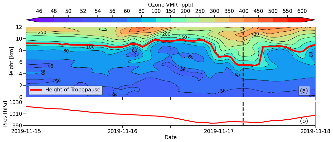
Figure 1 (a) Time–height cross section of the ozone volume mixing ratio (ppb) and 4 PVU dynamical tropopause height (red curve) from ERA5. (b) Corresponding surface pressure from ERA5. The data are at the Polarstern location from 15 to 18 November 2019 (Event 1). The black dashed line marks the specific time mentioned in the text.

Figure 2 The same as Fig. 1 but for the period from 30 January to 2 February 2020 (Event 2).

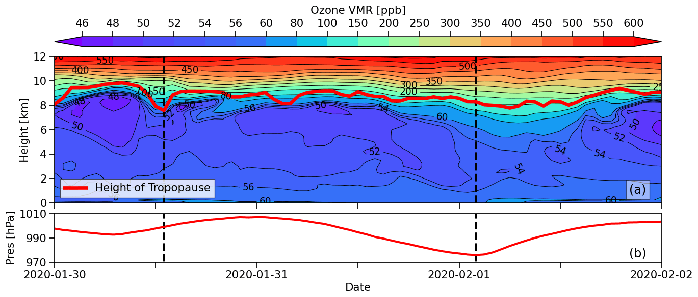
For the untypical Event 2, as illustrated in Fig. 2, the correlation between ozone content and tropopause height is much less pronounced but is still visible. For example, at 13:00 UTC on 30 January (marked as a dashed black line in Fig. 2), the tropopause lowers from around 10 to 8 km, together with the corresponding ozone VMR level of 100 ppb from around 9 to 8 km. This lowering can possibly be attributed to another preceding cyclone that impacted Polarstern at 07:00 UTC on 30 January. In addition, there is no visible disturbance of the tropopause near the centre of the second minimum of surface pressure at 02:00 UTC on 1 February (marked as a dashed black line in Fig. 2).

Figure 3 The same as Fig. 1 but for the period from 15 to 18 April 2020 (Event 3).

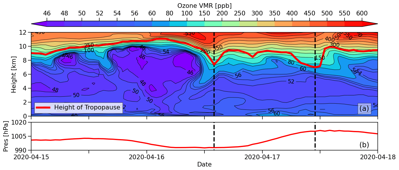
For the untypical Event 3, however, the tropopause is lowered near the minimum of the surface pressure at 14:00 UTC on 16 April (marked as a dashed black line in Fig. 3). The tropopause moves down from about 11 to 7.5 km. The correlation between the tropopause and the ozone content still exists as the ozone VMR level of 150 ppb moves down from around 10 to 7.5 km. In contrast, a minimum in tropopause height is seen later near a maximum in surface pressure at around 12:00 UTC on 17 April (marked as a dashed black line in Fig. 3), suggesting that the tropopause disturbance is decoupled from the surface pressure.

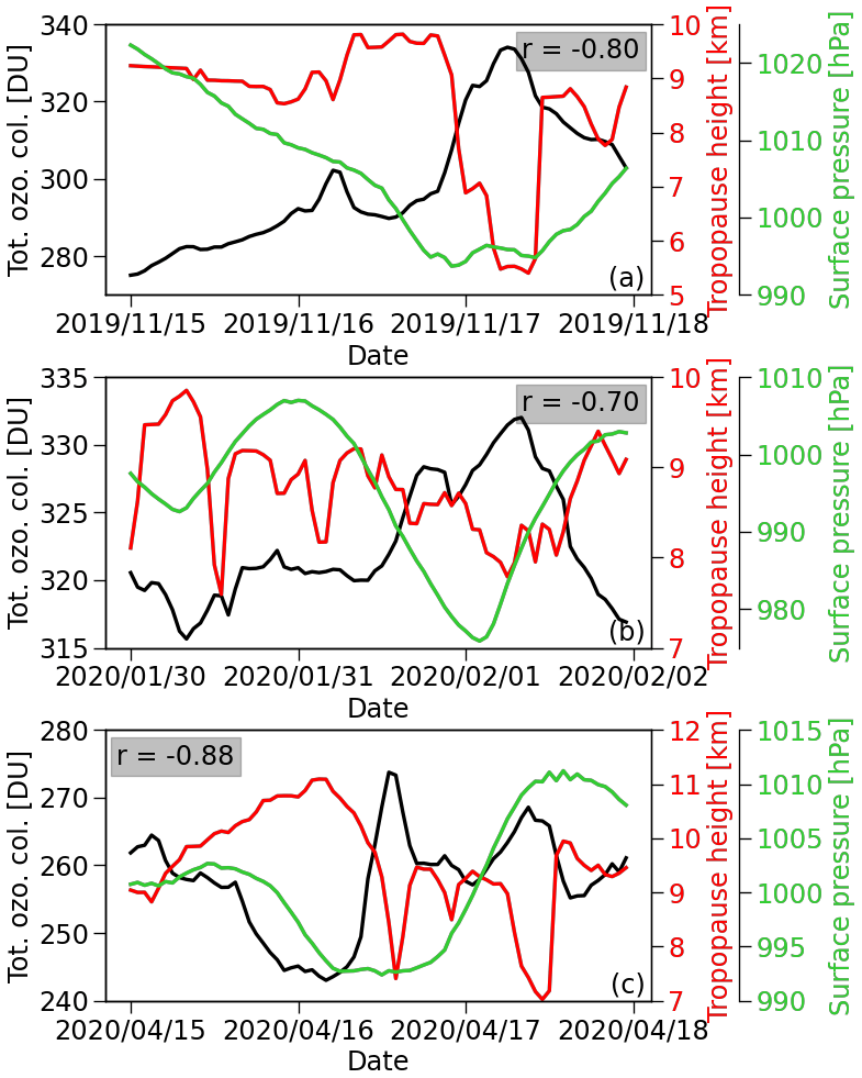
Figure 4 Total ozone column (black), 4 PVU dynamical tropopause height (red), and surface pressure (green) from ERA5 at the Polarstern positions of (a) Event 1, (b) Event 2, and (c) Event 3. The shown correlation coefficient indicates the correlation between total ozone column and 4 PVU dynamical tropopause height.

Figure 4 shows the evolution of the total ozone column, the 4 PVU dynamical tropopause, and the surface pressure, all from ERA5, for the three events. Again, the surface pressure is shown as an indicator of the cyclone. For all of the events, the expected negative correlation between the total ozone column and the tropopause height can be seen. Consequently, for Event 1, we have a negative correlation of $r=-\mathrm{0.80}$ and the highest ozone column at the location of the cyclone (Fig. 4a, 17 November, 06:00 UTC). The total ozone column increases from 290 DU (16 November, 12:00 UTC) to 334 DU (17 November, 06:00 UTC), and the tropopause moves down from approximately 10 to 5.5 km during this event. Figure 4b shows better than Fig. 2 that, also for Event 2, which is classified as untypical, a slight lowering of the tropopause of about 1 km occurs at 04:00 UTC on 1 February. At this point, the total ozone column is at its maximum, rising from approximately 325 DU (23:00 UTC on 31 January) to 332 DU (10:00 UTC on 1 February). The negative correlation is slightly lower compared to Event 1, with a correlation coefficient of $r=-\mathrm{0.70}$. For Event 3 (Fig. 4c), we have the highest absolute correlation of the three events ($r=-\mathrm{0.88}$) and the highest total ozone column change, rising from approximately 243 DU (04:00 UTC on 16 April) to 274 DU and coinciding with a local minimum of the tropopause (14:00 UTC on 16 April).

3.2 Extended analysis of tropopause–ozone linkage during the MOSAiC summer

Due to the fact that tropopause lowering can be detected during normal and untypical cyclone events, although the strength of the lowering varies, we assume that most cyclone events can be identified from a change in tropopause height. Therefore, the question arises as to what extent satellite ozone data can be used for the detection of tropopause-induced ozone changes.

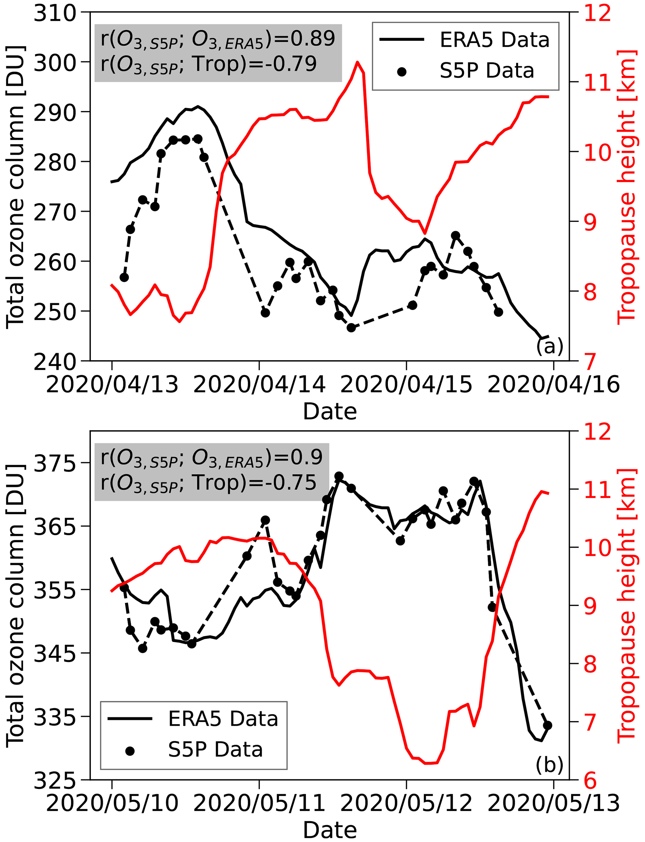
Figure 5 Total ozone column from ERA5 and S5P data and 4 PVU dynamical tropopause height from ERA5 at the Polarstern positions for (a) a rising tropopause in April 2020 and (b) a descending tropopause in May 2020.

3.2.1 S5P and TROPOMI total ozone columns

To start off with the analysis of the S5P satellite ozone data, two different cases of tropopause movement were used to consider both a tropopause rising and a tropopause lowering (Fig. 5). The rising tropopause (anticyclone) took place in April 2020, and the lowering tropopause (cyclone) took place in May 2020. When comparing the total ozone column from ERA5 and S5P, we see good qualitative agreement and a high correlation between both data sets (r=0.89 for the case in April and r=0.90 for the case in May 2020, respectively). One can observe that, for the anticyclone-induced tropopause rise (Fig. 5a), which occurred from 13 to 15 April 2020, an expected decrease in the S5P total ozone column was observed. The tropopause rises from about 8 to 11 km and the total ozone column from ERA5 and S5P drops from about 290 to 250 DU. The same correlation is shown for the cyclone-induced descending tropopause (Fig. 5b), which occurred from 11 to 13 May 2020, when we have an increase in the S5P and ERA5 total ozone columns. The tropopause decreases from approximately 10 to 6 km and the total ozone column increases from approximately 350 to 370 DU. In addition, there is a high overall anti-correlation between the 4 PVU dynamical tropopause height from ERA5 and the total ozone column from S5P for both 3 d periods ($r=-\mathrm{0.78}$ in April and $r=-\mathrm{0.76}$ in May).

To make a more robust statement about the correlation between the S5P total ozone column and the ERA5 dynamical tropopause height, a scatterplot for the 3-month period June–August 2020 at the Polarstern position is shown in Fig. 6a. This time period was chosen to make the evaluation comparable with the evaluation of the OMPS-LP data, which only has observations at the Polarstern position from June onwards due to the long polar nights, the smaller swath of the instrument, and the northern position of Polarstern. For the same reason, data north of 81.3° N are coloured red and are not included in the correlation analysis of tropopause height vs. S5P ozone. Most of the red data points found in the 240–280 DU range deviate from the correlation line and occur in August 2020. This is most likely due to the minimum stratospheric dynamic activity at the end of summer (e.g. Weber et al., 2011). The satellite measurements and ERA5 data were required to be collocated within ranges of ±111 km and ±15 min around the Polarstern positions. This enables us to compare the satellite results with MOSAiC ozonesonde data, as shown later (Sect. 4.2.3). The anti-correlation between the ERA5 tropopause height and the S5P total ozone column still remains high, with a correlation coefficient of $r=-\mathrm{0.83}$. Comparing the total ozone column from ERA5 and S5P data (Fig. 6b), ERA5 tends to underestimate the observed total ozone column at higher values, but very good agreement between the two data sets at the Polarstern positions is still evident. A high correlation coefficient of r=0.96 underlines the suitability of gap-free ERA5 ozone data for a long-term analysis of the connection between cyclones and ozone in the Arctic.

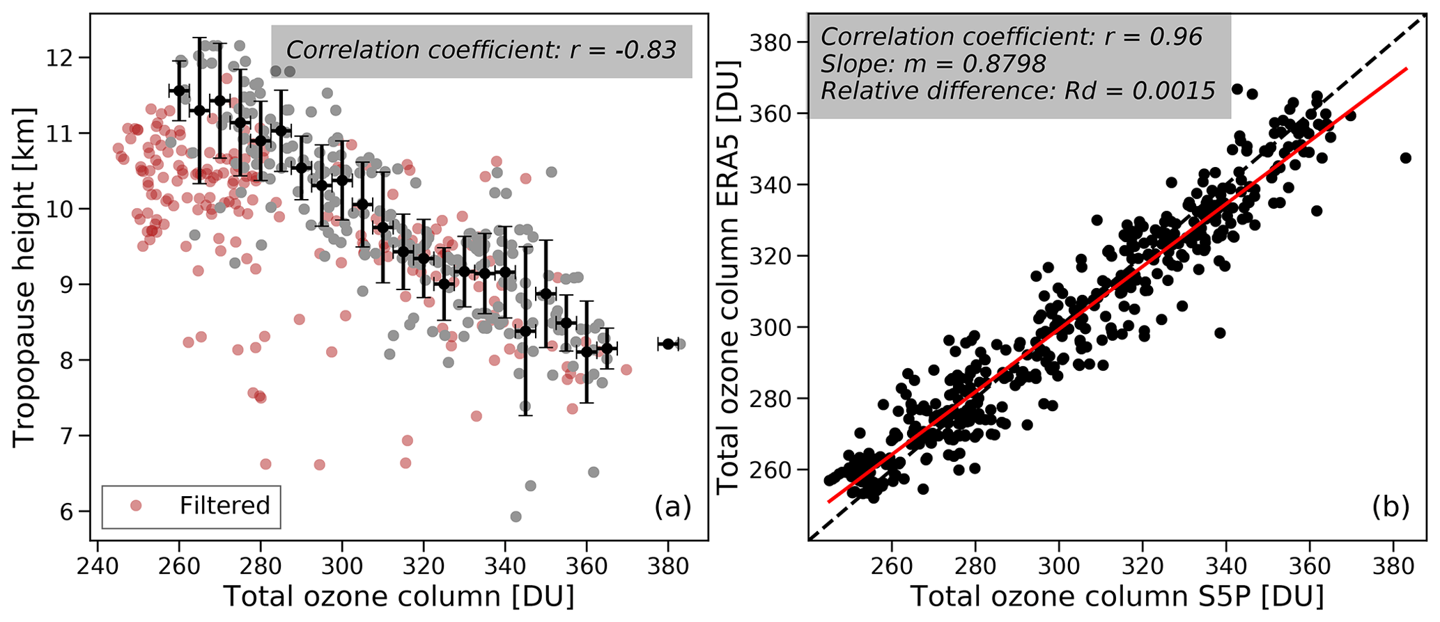
Figure 6 Scatterplots: (a) 4 PVU dynamical tropopause height from ERA5 vs. total ozone from S5P (grey and red data points). Data measured after 08:00 UTC on 15 August 2020 and data north of 81.3° N are coloured red, for which OMPS-LP data are not available. All other data points are shown in grey and used to determine the correlation coefficient. The black data points are averages in 5 DU bins of the grey data with vertical standard deviations as error bars. (b) Scatterplot of ERA5 and S5P total ozone columns. The data are at the Polarstern location during June–August 2020.

3.2.2 OMPS-LP ozone profiles

For this analysis, the time period of June to August 2020 was considered. As explained earlier, OMPS-LP ozone data are only available for latitudes below 81.3° N during this period. No OMPS-LP data collocated with the MOSAiC ship campaign were available after mid-August 2020. OMPS-LP measurements within a ±555 km range around Polarstern and within a range of ±30 min around MOSAiC-collocated ERA5 data were selected. Figure 7 shows the partial ozone column from 10 to 20 km from ERA5 and OMPS-LP along with the 4 PVU tropopause height. The partial ozone column from 10 to 20 km was used here because the tropopause height change has the highest influence on ozone in this altitude region, as discussed in more detail below. OMPS-LP is in good qualitative agreement with the ERA5 ozone and has a high correlation of r=0.87. Moreover, a high anti-correlation ($r=-\mathrm{0.64}$) between the partial ozone column from OMPS-LP and the ERA5 dynamical tropopause height is evident, especially on 24 June and 12 July 2020. During the June event, the tropopause height rises to 11.1 km and the partial ozone column from OMPS-LP falls to 80 DU. This effect is even stronger during the July event, with a tropopause height of 12 km and a low partial ozone column of 66 DU.

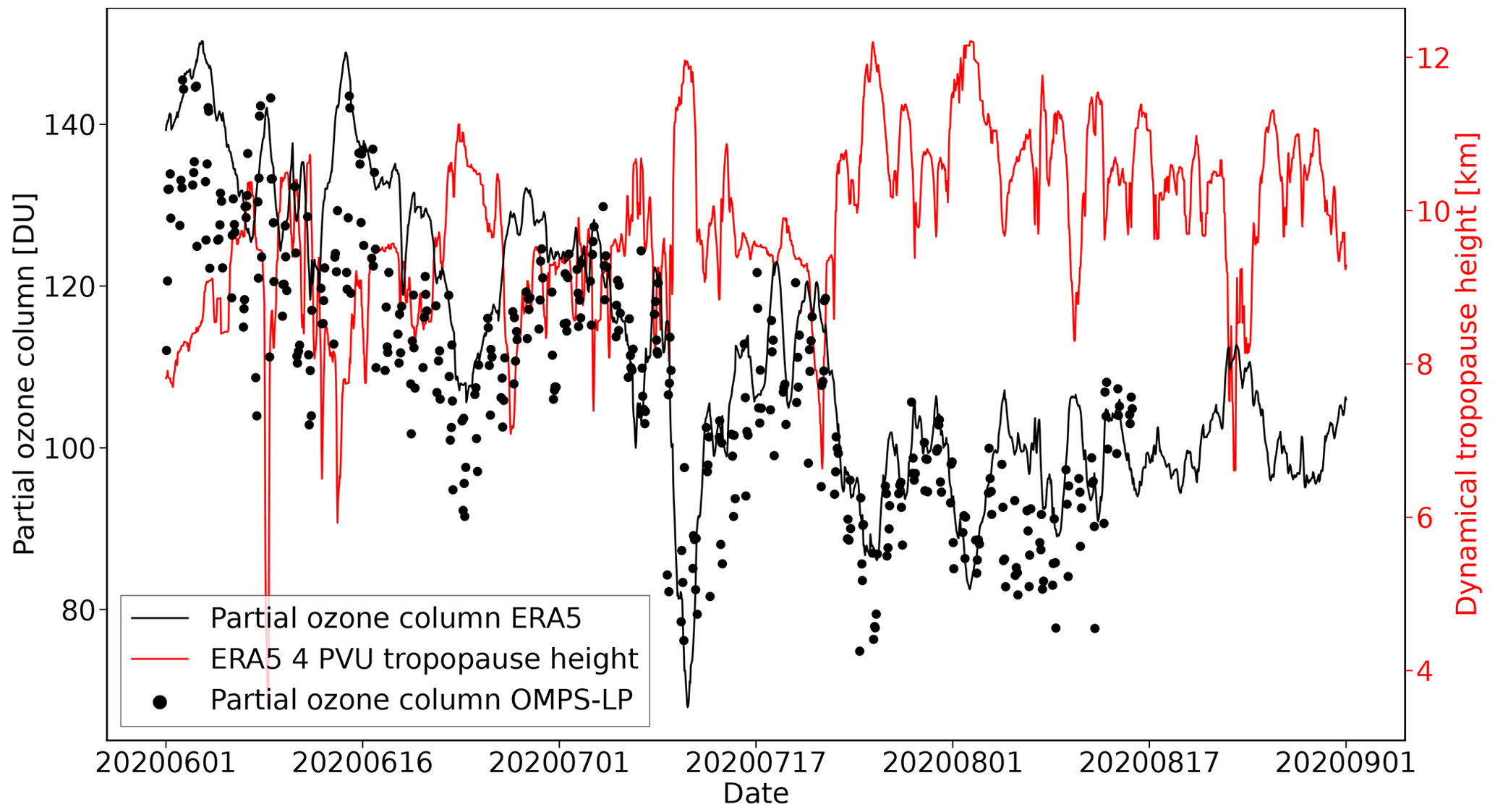
Figure 7 Partial ozone column in the altitude range 10–20 km from OMPS-LP and ERA5 and the ERA5 4 PVU dynamical tropopause height from June to August 2020 at the Polarstern position.

In order to find out which height region of ozone is most affected by tropopause height changes, partial ozone columns in different altitude ranges (10–20, 20–30, 30–60, and 10–60 km) are plotted against the ERA5 4 PVU dynamical tropopause height in Fig. 8. The highest correlation ($r=-\mathrm{0.72}$) occurs for ozone columns in the 10–20 km range, which is expected because of the proximity to the tropopause. The influence of the tropopause height on the ozone contour levels decreases with increasing altitude (James et al., 1997). The correlation coefficient decreases to $r=-\mathrm{0.44}$ in the 20–30 km height range and is even lower ($r=-\mathrm{0.27}$) above in the 30–60 km height range. The correlation for the total ozone column, which is closely represented by the height range from 10 to 60 km (panel d), is nearly as high as the correlation in the 10–20 km range with a correlation coefficient of $r=-\mathrm{0.69}$. This correlation is somewhat lower than for S5P columns due to the more relaxed collocation criteria used for OMPS-LP to obtain a sufficient number of collocated OMPS-LP observations. If the same collocation criteria are used for S5P with a limit of ±555 km, a correlation coefficient of $r=-\mathrm{0.53}$ is obtained.

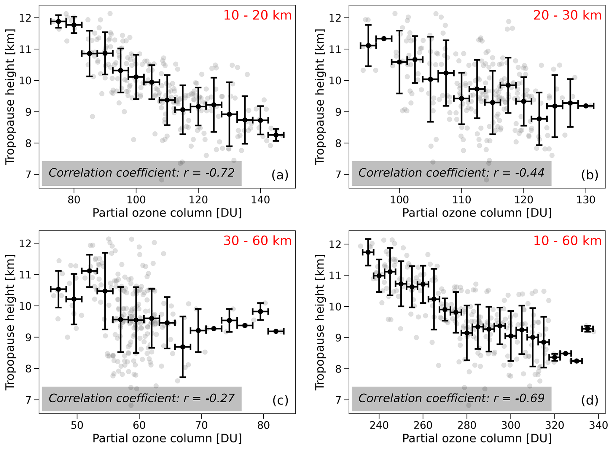
Figure 8 ERA5 4 PVU dynamical tropopause height vs. OMPS-LP ozone sub-columns in the altitude ranges 10–20 (a), 20–30 (b), 30–60 (c), and 10–60 km (d) at the Polarstern location from June to August 2020 (grey data points). The black data points are averages in 5 DU bins of the grey data with vertical standard deviations as error bars. The grey data points were used to determine the correlation coefficients.

3.2.3 MOSAiC ozone profile data

Figure 9a shows the correlation between the ERA5 4 PVU dynamical tropopause height and the ozone sub-column (0 to 25 km) from MOSAiC ozonesondes for September 2019 to October 2020. There were a total of 49 ozonesondes launched during the entire MOSAiC campaign that measured ozone at an altitude of at least 25 km. The correlation between the tropopause height and the ozone column is lower compared to OMPS-LP and S5P, with a correlation coefficient of only $r=-\mathrm{0.51}$, which can be due to finer structures seen by the ozonesondes, their intrinsic measurement noise, or the fact that most of the ozonesonde launches were carried out on days when there were no cyclones above Polarstern (Fig. 10). If we calculate the correlation between the ERA5 partial ozone column from 0 to 25 km and the ERA5 dynamical tropopause height for the same locations and times as the MOSAiC ozonesonde launches, we get the same lower correlation of $r=-\mathrm{0.51}$, which implies that the absence of cyclones is the main reason for the lower correlation. Comparing the integrated ozone columns from 0 to 25 km from ERA5 and MOSAiC (Fig. 9b), a high correlation (r=0.94) was found. The ERA5 data systematically overestimate the ozonesonde columns by about 1.9 %.

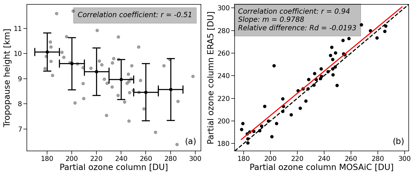
Figure 9 Scatterplots: (a) 4 PVU dynamical tropopause height from ERA5 vs. the ozonesonde sub-columns (0–25 km) from MOSAiC. The black data points are averages in 20 DU bins of the grey data with vertical standard deviations as error bars. The correlation was determined from the grey points; (b) ERA5 vs. MOSAiC ozonesonde sub-columns (0–25 km).

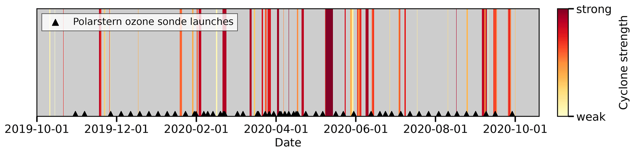
Figure 10 All cyclone events (vertical bars) as a function of time that impacted Polarstern and that were classified in Rinke et al. (2021) are colour-coded according to the cyclone strength (see the main text for a definition). The bar widths represent the lifetimes of the individual cyclones. The days where ozonesondes were launched from Polarstern are marked by black triangles at the bottom.

3.3 Cyclone identification with OMPS-LP ozone data

With the knowledge that most cyclone events are associated with a lowering of the tropopause and that the largest impact of tropopause height change on ozone is observed in the 10–20 km range, our next step was to investigate the connections between cyclones and OMPS-LP stratospheric ozone data in more detail. Such connections can be used as a diagnostic tool to investigate long-term changes in cyclone activity and in the future as a potential input for data assimilation in numerical weather prediction models. Our objective, therefore, is to investigate how much information about cyclones is available in the stratospheric OMPS-LP data. In order to find suitable cyclones for a first investigation using the OMPS-LP data, we looked at cyclone events identified during the MOSAiC campaign. All cyclones that passed over Polarstern during the MOSAiC campaign were classified in Rinke et al. (2021). An overview of the cyclones with their corresponding strengths is shown in Fig. 10. The cyclone strength or depth is defined as the difference between the surface pressure at the centre of the cyclone and the surface pressure at the edge of the cyclone. The weakest and strongest cyclones had depths of 1.57 and 44 hPa, respectively (Fig. 10). The cyclone from 7 to 13 May 2020 was not only the one with the longest lifetime during the MOSAiC campaign, but it was also the one with the highest cyclone depth of 44 hPa. Although there were no ozonesonde launches during this event, both ERA5 data and OMPS-LP ozone data were available to investigate this cyclone.

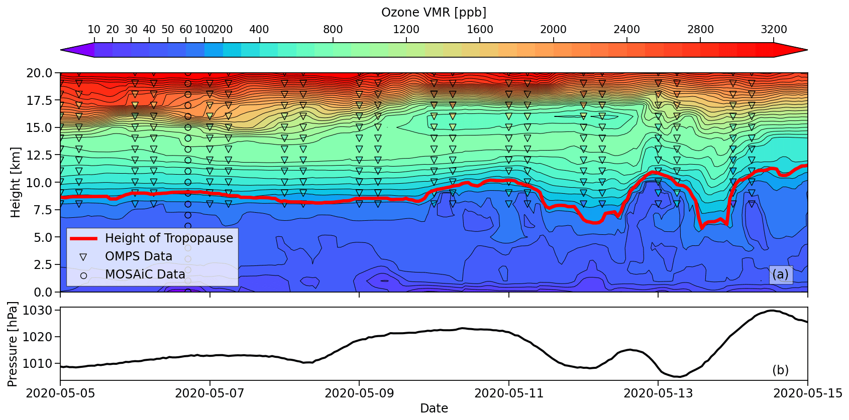
Figure 11 (a) Time–height cross section of the ozone volume mixing ratios (ppb) from the ERA5 (colour shading), OMPS-LP, and MOSAiC ozonesondes, together with the dynamical 4 PVU tropopause height. The MOSAiC (circles) and OMPS-LP (triangles) ozone data have the same colouring as the contours of the ERA5 data. (b) Surface pressure from ERA5 at the Polarstern positions. Note the different colour range with respect to Figs. 1–3.

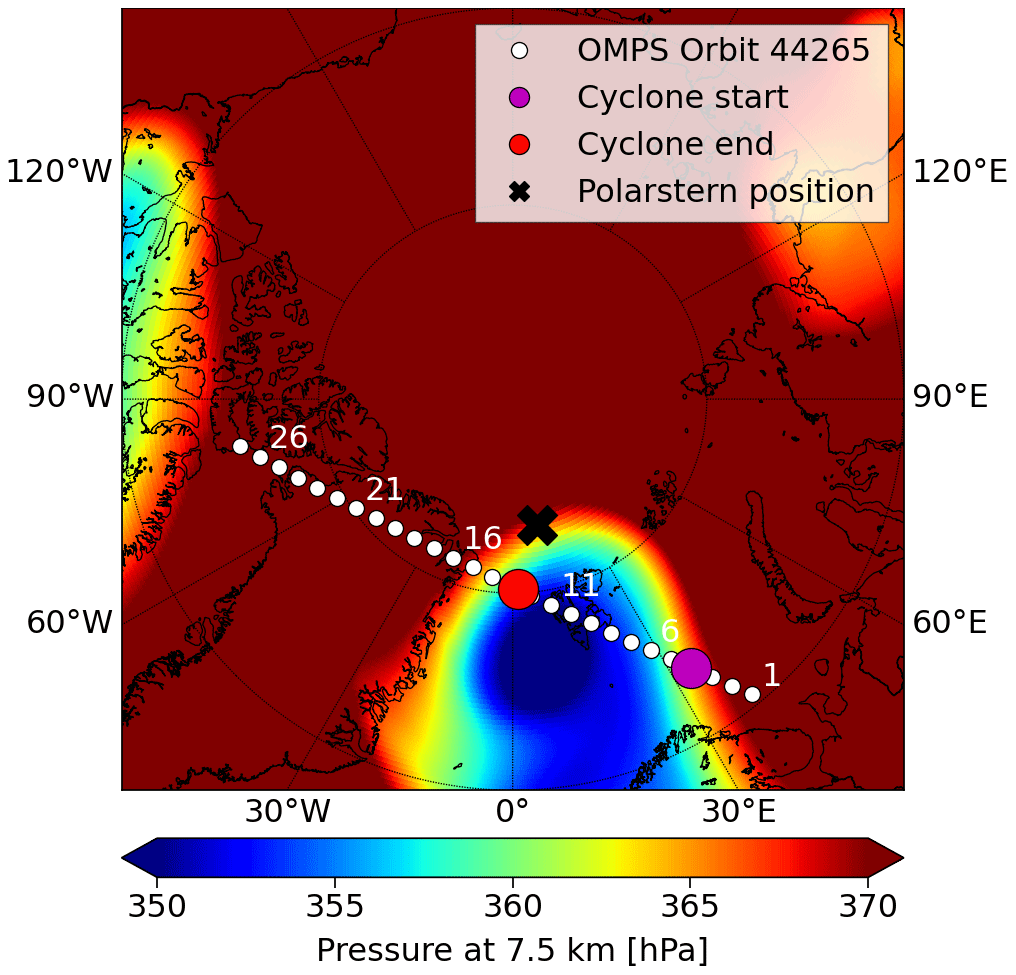
Figure 12 Pressure at 7.5 km from ERA5 in the Arctic at 09:00 UTC on 13 May 2020. The Polarstern position (black cross), the cyclone borders that were calculated using the ozonopause from OMPS-LP (big coloured dots), and the OMPS-LP measurement points along orbit 44 265 (small white dots) are shown.

Figure 11 shows the time–height cross section of the ozone VMR from the ERA5, OMPS-LP, and MOSAiC ozonesondes, the dynamical 4 PVU tropopause height, and the surface pressure from the ERA5 data from 5 to 15 May 2020. Although the average deviation between the OMPS-LP and ERA5 data is about 33 %, we still see overall agreement between these two data sets in this time period. The data from the ozonesonde from Polarstern on 6 May agree well with the ERA5 data, with an average deviation of around 10 %. The cyclone impacts Polarstern on three occasions during this period: 8, 12, and 13 May. The first occurrence is associated with only a small dip in the tropopause height and has no visible disturbance in the ozone field. The second and third occurrences, on the other hand, are associated with a tropopause lowering of about 3–4 km associated with ozone contour levels descending in the altitude region between the tropopause and up to about 12 km for the second occurrence and 17 km for the third occurrence. For the third occurrence there is also a time delay of about 12 h between the minimum of the surface pressure and the downward motion of the tropopause and ozone.

To evaluate the influence of this cyclone on the UTLS ozone, one OMPS-LP orbit crossing the cyclone was selected (Fig. 12). The start and end points of the cyclone crossing as determined from the ozonopause are also shown. The method for their determination is discussed below. Figure 13 shows the time–height cross section of the ozone VMR from this OMPS-LP orbit (orbit number 44 265) and the corresponding pressure at 7.5 km altitude from ERA5. Pressure at 7.5 km will be used to identify the cyclone instead of the surface pressure, on the one hand because of the increasing surface altitude over Greenland (which strongly influences the surface pressure) and on the other hand because in this altitude range we observe the highest cyclone-induced drop in pressure. As discussed before, ozone contour levels up to 15 km are influenced by the cyclone (Fig. 13). Due to the fact that OMPS-LP data are not available below 8 km altitude, descending ozone below this altitude is not visible in the figure.

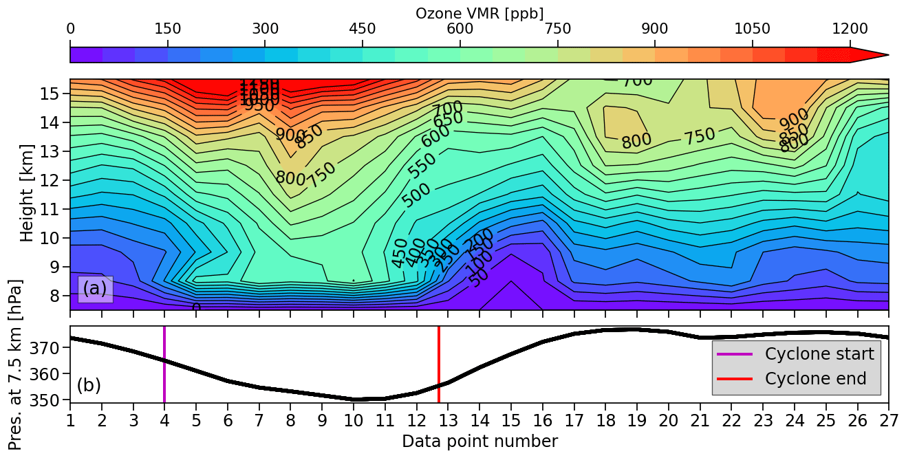
Figure 13 (a) Time–height cross section of the ozone volume mixing ratio (ppb) from OMPS-LP orbit 44 265 at 09:00 UTC on 13 May 2020. (b) Corresponding pressure at 7.5 km altitude with the cyclone borders derived from the ozonopause from OMPS-LP data (see the main text). The x axis is defined by the measurement point number of the partial OMPS-LP orbit.

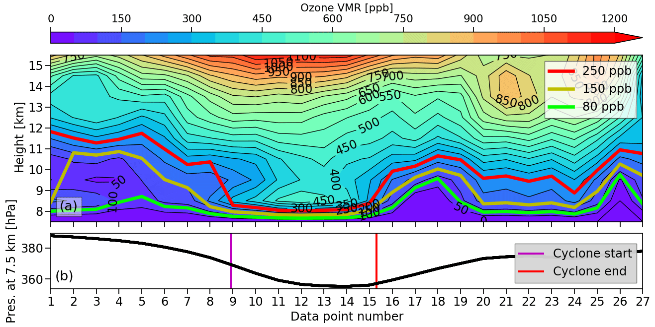
Figure 14 (a) Time–height cross section of the ozone volume mixing ratio (ppb) from OMPS-LP orbit 44 264 at 07:00 UTC on 13 May 2020. Different ozone levels (80, 150, and 250 ppb) are shown. (b) Pressure at 7.5 km with the cyclone borders that were calculated from the 250 ppb ozone level going below 9 km (see the main text). The x axis is defined by the measurement point number along the OMPS-LP orbit.

Ozone contour levels at altitudes between 8 and 15 km are most strongly influenced by cyclones, and their vertical movement can be tracked using OMPS-LP data. This can be exploited for automated identification of cyclone boundaries by tracing the movement of a certain ozone level. Different ozone VMR thresholds for defining the ozonopause were tested. To illustrate their differences, Fig. 14a shows the time–height cross section of the OMPS-LP ozone volume mixing ratio from orbit 44 264 (which is the orbit preceding the one shown in Fig. 13) on 13 May 2020 and selected ozone contour levels (80, 150, and 250 ppb) as candidates for the ozonopause. Figure 14b again shows the pressure at 7.5 km with cyclone borders of the same cyclone event as illustrated in Fig. 13. Here, a previous OMPS-LP orbit with respect to that shown in Fig. 13 is shown to better illustrate issues related to the use of the lower ozone layer to define the tropopause. We note that the 250 ppb contour best follows the cyclone-induced ozone movement. The main reason is that the OMPS-LP data below 8 km are not retrieved, while ozone contours of 80 and 150 ppb can be located below that altitude. In this case we would not see additional lowering of ozone contour levels, meaning that the 80 and 150 ppb ozone contour levels related to cyclones cannot be observed. The use of the 250 ppb contour as the ozonopause is, therefore, more suitable as it is low enough in altitude to be impacted by most cyclones but high enough to have continuous reliable data from OMPS-LP.

The location where the 250 ppb ozone level falls below 9 km altitude was selected to define the extent of the cyclone. An altitude of 9 km was used because the 250 ppb contour normally lies between 10 and 12 km. To mitigate the influence of stratospheric streamers and other possible errors, we introduce the criterion that the ozone contour level of 250 ppb has to be below 9 km for at least five consecutive measurements of OMPS-LP (approximately 1500 km along the orbit) in order to qualify as a cyclone event. When applying this criterion to OMPS-LP orbit 44 265 (Figs. 12 and 13), we see that the ozone-defined borders of the cyclone are reasonably defined when compared to the ERA5 pressure at 7.5 km. Although the end of the cyclone seems to be somewhat too early, the main structure and strongest region of the cyclone are captured well using our ozone criterion.

Another case study of a cyclone event on 4 May demonstrates the usefulness of our ozone criterion as illustrated in Fig. 15. This case was selected because there were three OMPS-LP orbits within 4 h that crossed the cyclone. These three consecutive OMPS-LP orbits were used to determine the cyclone borders. For all three orbits, there is good qualitative agreement between the structure of the cyclone from ERA5 pressure data and the cyclone borders from the motion of the OMPS-LP 250 ppb ozone level. This illustrates that the motion of a cyclone can be traced using only OMPS-LP ozone data, provided there are sufficient OMPS-LP orbits crossing the cyclone.

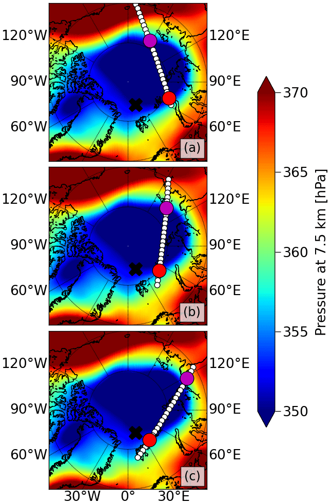
Figure 15 Pressure at 7.5 km for the cyclone event at (a) 00:00 UTC, (b) 02:00 UTC, and (c) 04:00 UTC on 4 May 2020. The positions of the OMPS-LP measurement points of the corresponding OMPS-LP orbits and the calculated cyclone borders are marked (Fig. 12).

4 Summary and conclusions

When assimilating data in numerical weather prediction models, the use of ozone data has the potential to compensate for a sparsity of meteorological observations, which is typical for the Arctic region. In this paper, we investigated the ability of satellite ozone data to analyse cyclone events in this region. We introduced a method for cyclone diagnostics using satellite ozone data. The connection between the total ozone columns and cyclone events was validated using the ERA5 4 PVU dynamical tropopause. The connection between tropopause changes and the S5P total ozone column was confirmed not only for two case studies in April and May, but also for a 3-month period in the Arctic. This relationship was also investigated with MOSAiC ozonesonde and OMPS-LP sub-columns. A lower correlation was found for the MOSAiC ozonesondes due to the sparsity of data and the absence of ozonesonde launches during cyclones. Using the vertically resolved profiles from OMPS-LP enabled us to study the influence of tropopause height changes in different altitude ranges. As expected, the highest influence occurred at an altitude of 10 to 20 km (lowermost stratosphere). This influence was also confirmed with ERA5 pressure and ozone data for three cyclone events during the MOSAiC campaign. Contours of constant ozone VMR in the UTLS region follow the course of the descending tropopause during the cyclone events. Even in the case of untypical cyclone events (Rinke et al., 2021), a weak lowering of the tropopause was found above the cyclone. In one case, a time lag in the subsidence of several hours after the surface pressure minimum during the MOSAiC campaign was noted, which requires further investigation. Significant correlation and good agreement between ozone data from the OMPS-LP, S5P, and MOSAiC ozonesondes and ERA5 ozone were shown, indicating that ERA5 ozone is suitable for long-term analysis. ERA5 has the advantage that it is gap-free and covers a long period (at least since 1978), and there is no limitation due to the polar night like for OMPS-LP and S5P. These advantages enable us to identify further characteristics of the relationship between cyclones and ozone in the Arctic, which need to be verified by space-borne ozone data.

A method for determining cyclone borders was developed using OMPS-LP ozone. The criterion that the cyclone boundary can be defined where the 250 ppb ozone level falls below 9 km was found to be a reasonable choice. The main rationale here is the fact that cyclone-induced changes in the tropopause height affect ozone above the tropopause through horizontal advection. This method was applied in two case studies using ERA5, MOSAiC ozonesondes, and OMPS-LP data. One event, according to Rinke et al. (2021) the strongest cyclone event during the MOSAiC campaign, was identified using OMPS-LP ozone observations. For the other one on 4 May, the cyclone border was properly identified in three consecutive OMPS-LP orbits.

Since this method has so far only been tested on cyclones, the question arises as to what extent the method is also suitable for other synoptic events (e.g. anticyclones), which needs further studies. It should be noted that this is only the first approach and that the method may require additional analyses and improvements. For example, stratospheric streamers or other non-cyclone-based ozone motions may cause the 250 ppb level to drop below 9 km for a horizontal length of over 1500 km. In addition, the polar vortex has to be taken into account to reliably use ozonopause motion to evaluate cyclones.