Overview: quasi-Lagrangian observations of Arctic air mass transformations – introduction and initial results of the HALO–(𝒜 𝒞)³ aircraft campaign

Global warming is amplified in the Arctic. However, numerical models struggle to represent key processes that determine Arctic weather and climate. To collect data that help to constrain the models, the HALO–(𝒜𝒞)³ aircraft campaign was conducted over the Norwegian and Greenland seas, the Fram Strait, and the central Arctic Ocean in March and April 2022. The campaign focused on one specific challenge posed by the models, namely the reasonable representation of transformations of air masses during their meridional transport into and out of the Arctic via northward moist- and warm-air intrusions (WAIs) and southward marine cold-air outbreaks (CAOs). Observations were made over areas of open ocean, the marginal sea ice zone, and the central Arctic sea ice. Two low-flying and one long-range, high-altitude research aircraft were flown in colocated formation whenever possible. To follow the air mass transformations, a quasi-Lagrangian flight strategy using trajectory calculations was realized, enabling us to sample the same moving-air parcels twice along their trajectories. Seven distinct WAI and 12 CAO cases were probed. From the quasi-Lagrangian measurements, we have quantified the diabatic heating/cooling and moistening/drying of the transported air masses. During CAOs, maximum values of 3 K h⁻¹ warming and 0.3 g kg⁻¹ h⁻¹ moistening were obtained below 1 km altitude. From the observations of WAIs, diabatic cooling rates of up to 0.4 K h⁻¹ and a moisture loss of up to 0.1 g kg⁻¹ h⁻¹ from the ground to about 5.5 km altitude were derived. Furthermore, the development of cloud macrophysical (cloud-top height and horizontal cloud cover) and microphysical (liquid water path, precipitation, and ice index) properties along the southward pathways of the air masses were documented during CAOs, and the moisture budget during a specific WAI event was estimated. In addition, we discuss the statistical frequency of occurrence of the different thermodynamic phases of Arctic low-level clouds, the interaction of Arctic cirrus clouds with sea ice and water vapor, and the characteristics of microphysical and chemical properties of Arctic aerosol particles. Finally, we provide a proof of concept to measure mesoscale divergence and subsidence in the Arctic using data from dropsondes released during the flights.

1 Introduction

In 2017, anthropogenic warming quantified by the globally and annually averaged near-surface air temperature reached around 1 K above the pre-industrial level (Masson-Delmotte et al., 2021). In 2022, the human-induced warming averaged 1.26 K over the decade 2013–2022 (Forster et al., 2023). For 2023, the data published by the Copernicus Climate Change Service show that on almost 50 % of days in that year the anthropogenic warming exceeded the values of the pre-industrial period (1850–1900) by at least 1.5 K (https://climate.copernicus.eu/global-climate-highlights-2023, last access: 6 August 2024). The advancing global warming triggers numerous feedback mechanisms within the Earth's climate system, most of which are not fully accounted for in corresponding numerical models (Ripple et al., 2023). Of the 41 important feedback loops identified by Ripple et al. (2023), at least a quarter cause distinct, mainly amplifying, effects in the Arctic. Prominent examples of these Arctic-relevant feedback mechanisms are the Planck, water vapor, surface albedo, and cloud effects. This makes the Arctic one of the “hot spots” of global climate change (Overland et al., 2011).

One obvious indication of Arctic amplification is the up to 4 times faster increase in Arctic near-surface air temperature compared to global warming over the last 3–4 decades, which fits only poorly into the scatter of the multi-model ensemble results of the Coupled Model Intercomparison Project (CMIP), Phase 5 (CMIP5) and Phase 6 (CMIP6) (Holland and Landrum, 2021; Rantanen et al., 2022; Chylek et al., 2022). Further obvious signs of Arctic amplification are the faster-than-expected and remarkable decline in the sea ice cover of the Arctic Ocean since around 1970, especially in late summer (Stroeve et al., 2007; Olonscheck et al., 2019; Serreze and Meier, 2019; Screen, 2021), and the thawing of the permafrost soils (Beer et al., 2020). These changes have important consequences for the living conditions of the local Arctic human population, as well as for the flora and fauna of the Arctic. They also imply potentially far-reaching economic impacts for fishing in Arctic waters, transoceanic shipping routes, tourism, and the extraction of natural resources (Melia et al., 2016; Alvarez et al., 2020).

Arctic amplification has long been understood to be a feature of global climate change (Manabe and Wetherald, 1975). More recently, knowledge and understanding of the processes and feedback mechanisms governing Arctic amplification have improved considerably (Previdi et al., 2021; Smith et al., 2021; Taylor et al., 2022; Wendisch et al., 2023). Nevertheless, the current ability to model them is still limited, and therefore, future model-based projections of Arctic climate changes are highly uncertain (Smith et al., 2019; Cohen et al., 2020; Block et al., 2020; Linke et al., 2023). In particular, the model representations of the effects and development of clouds (Pithan et al., 2014; Wendisch et al., 2019; Kretzschmar et al., 2020; Stevens and Kluft, 2023) and of the interactions of the atmosphere with sea ice, snow on sea ice, and ocean physics, as well as biogeochemical feedback processes, are challenging (Rinke et al., 2019; Huang et al., 2019; Pefanis et al., 2020). In addition, the role of aerosol particles in Arctic amplification has not been sufficiently investigated (Schmale et al., 2021; Dada et al., 2022; Gong et al., 2023).

For more than a decade, there is some debate as to whether climate changes in the Arctic will impact the weather and climate in the mid-latitudes (Cohen et al., 2014). Several dynamic processes in the lower and upper troposphere and the stratosphere may lead to a weaker or stronger jet stream (Francis and Vavrus, 2015; Blackport and Screen, 2020; Yuval and Kaspi, 2020), with consequences for the meandering (amplitude) and persistence of the Rossby waves. These dynamical effects influence the meridional transport of heat, moisture, and momentum through northward warm-air intrusions (WAIs¹), including so-called atmospheric rivers (ARs) and southward cold-air outbreaks (CAOs²). More frequent WAIs could further enhance Arctic warming (Pithan et al., 2018; Nash et al., 2018), whereas CAOs may contribute to cold events in mid-latitudes. Recent studies suggest that despite the Arctic warming, cold-winter events in mid-latitudes have remained nearly as extreme and as common as decades ago (Cohen et al., 2023; Nygård et al., 2023). The results of the Polar Amplification Model Intercomparison Project (PAMIP) show very little evidence of linkages (Smith et al., 2022).

Rossby waves realize the meridional transport of air masses into and out of the Arctic. It is estimated that WAIs increase total column water vapor and cloud prevalence in the Arctic winter by about 70 % and 30 %, respectively (Johansson et al., 2017b). As a result, stronger thermal infrared downward radiation reduces the net surface radiative cooling and increase the near-surface air temperature in winter by about 5 K (Johansson et al., 2017a). This warming could trigger an earlier onset of melting and more melt ponds, which would reduce the surface albedo. In addition, particles and pollution are transported into the Arctic during WAIs, which may influence cloud properties (Bossioli et al., 2021).

In spite of the high impact they have on the Arctic climate, there are problems in modeling air mass transformations during meridional transport (Sato et al., 2016; Pithan et al., 2016; Dimitrelos et al., 2020). In particular, large-scale models have difficulties representing important thermodynamic processes driving Arctic air mass transformations, including the evolution of microphysical properties of mixed-phase clouds (Pithan et al., 2014; McCoy et al., 2015; Tan and Storelvmo, 2019), the development of turbulent fluxes under stable stratification (Tjernström et al., 2005; Holtslag et al., 2013; Gryanik and Lüpkes, 2023), and the response of snow-covered sea ice to atmospheric forcing (Pithan et al., 2023). These processes control the response of the Arctic to climatic forcing, and their realistic representation in models is crucial for understanding the behavior and feedback mechanisms of the Arctic climate system (Block et al., 2020; Taylor et al., 2022).

While the large-scale conditions that favor the development of CAOs can be well predicted on sub-seasonal timescales, a better understanding of when and how CAOs lead to the development of polar lows is necessary to predict these events which often have large impacts (Polkova et al., 2021). Furthermore, improvements to the observing system and in the understanding and model representation of small-scale synoptic features and processes are needed to advance polar predictions on daily to seasonal timescales (Jung et al., 2016). Moreover, given the lack of in situ observations, models are often evaluated using reanalysis data. However, the fidelity of such atmospheric reanalyses can suffer from a low number of assimilated observations, as well as biases inherited from its driving model (Tjernström and Graversen, 2009).

As a consequence, dedicated observations of WAIs and CAOs would be helpful to improve the model capabilities in order to realistically represent processes that determine air mass transformations during meridional transports into and out of the Arctic (Wendisch et al., 2021). Lagrangian measurements are well suited for this purpose. The Lagrangian approach assumes that the observations are made in relation to a coordinate system that moves together with the air mass. In this way, the changes in the properties of the same air parcel can be observed along its pathway. In contrast, the observations from an Eulerian perspective refer to a locally fixed coordinate system so that the properties of successive, different air parcels are measured from a fixed position as a time series. Previous observations of air mass transformations in the Arctic have mostly been conducted in the Eulerian framework at locally fixed, ground-based positions partly combined with ship, aircraft, or satellite data. Examples include case studies based on data from the Surface Heat Budget of the Arctic Ocean (SHEBA) (Uttal et al., 2002) and the Multidisciplinary drifting Observatory for the Study of Arctic Climate (MOSAiC) (Shupe et al., 2022; Kirbus et al., 2023; Svensson et al., 2023) ship expeditions. Due to the lack of geostationary satellite data, the development of Arctic cloud properties can only be analyzed by polar-orbiting satellite observations from a Eulerian perspective assuming stationary conditions (Murray-Watson et al., 2023). However, the Eulerian approach does not permit the required observations of temporal air-mass-transforming processes.

Only very few Lagrangian aircraft-based studies have been carried out in the past (Boettcher et al., 2021) and none in the Arctic. Some authors have combined local icebreaker and airborne or satellite observations within a Lagrangian framework by means of trajectories based on reanalysis (Tjernström et al., 2019; Ali and Pithan, 2020; You et al., 2021a; Kirbus et al., 2023; Mateling et al., 2023). Another approach was performed in earlier aircraft-based campaigns with measurements along the mean wind direction in CAO conditions and WAIs (Hartmann et al., 1997; Brümmer and Thiemann, 2002; Vihma et al., 2003; Lüpkes et al., 2012; Chechin et al., 2013). These authors have focused on the local development around the Fram Strait and the close marginal sea ice zone (MIZ) with measurements above sea ice and open ocean. A disadvantage was that this analysis had to assume stationary conditions. This strategy turned out to be helpful, e.g., for the analysis and development of turbulence parameterizations. They could be validated through using them in mesoscale models and comparing their results with the observations. But then it was always difficult to identify the impact of changing inflow conditions during the necessary 3–6 h model runs; this is a drawback which can be avoided by purely Lagrangian measurements. Furthermore, several studies use atmospheric reanalysis to identify and discuss WAIs or CAOs (You et al., 2021b; Kirbus et al., 2024).

Therefore, we have designed and conducted the HALO–(𝒜𝒞)³ aircraft campaign (HALO, High Altitude and Long Range Research Aircraft – (𝒜𝒞)³ Project on Arctic Amplification Climate Relevant Atmospheric and Surface Processes and Feedback Mechanisms; see https://halo-ac3.de/, last access: 6 August 2024). Based on the open issues in modeling air mass transformations during meridional transport into and out of the Arctic, the HALO–(𝒜𝒞)³ mission pursued two general objectives (Wendisch et al., 2021). The first was to jointly use HALO and the Polar 5 (P5) and Polar 6 (P6) research aircraft to perform “quasi-Lagrangian”³ observations of air mass transformations during WAIs and CAOs – an approach that has not been tried before in the Arctic. The second was to test the ability of numerical atmospheric models to reproduce the measurements taken from the aircraft. The benchmarked models can then, for example, be applied to investigate linkages between Arctic amplification and mid-latitude weather. This paper describes efforts carried out in support of the first objective.

The article is structured around five sections. After the Introduction (Sect. 1), the three research aircraft mainly utilized in our campaign and their instrumentation, as well as their partly colocated flight patterns, are described in Sect. 2. The unique quasi-Lagrangian measurement strategy successfully applied during the campaign is presented in Sect. 3. Some initial results from HALO–(𝒜𝒞)³ and ongoing analysis are discussed in Sect. 4. The following themes are elaborated: air mass transformations during WAIs and CAOs (Sect. 4.1), Arctic clouds (Sect. 4.2) and aerosol particles (Sect. 4.3), and a proof of concept to measure mesoscale divergence and subsidence in the Arctic (Sect. 4.4). A concise summary and a brief outlook are given in Sect. 5.

2 Aircraft, instrumentation, and flight pattern

Three research aircraft were mainly involved in the HALO–(𝒜𝒞)³ campaign: HALO (High Altitude and Long Range Research Aircraft), Polar 5 (P5), and Polar 6 (P6). HALO is operated by the German Aerospace Center (Deutsches Zentrum für Luft- und Raumfahrt, DLR). It was based in Kiruna (northern Sweden; geographical coordinates of 67.85° N, 20.22° E). The P5 and P6 were stationed at Longyearbyen (Svalbard, Norway; 78.24° N, 15.49° E). These two aircraft belong to the Alfred Wegener Institute, Helmholtz Center for Polar and Marine Research (AWI). In addition, the British Facility for Airborne Atmospheric Measurements (FAAM) and the French Avions de Transport Régional (ATR) aircraft were concurrently based in Kiruna, measuring partly in coordination with HALO, P5, and P6. The ATR was operating from 22 March to 3 April 2022 and had some similar objectives to HALO–(𝒜𝒞)³ but with the addition of using in situ water isotope measurements to characterize processing of water vapor in these weather systems. The FAAM aircraft operated from 7 March to 1 April 2022 and focused on making in situ measurements of the development of CAOs from the sea ice around Svalbard to the Scandinavian coastline. FAAM was fitted with a range of instrumentation to measure the thermodynamic, aerosol, cloud, and precipitation properties within CAOs. Furthermore, intensive ground-based measurements were carried out at the permanent German–French AWIPEV research base operated by the AWI and the French Polar Institute Paul-Émile Victor (IPEV) at Ny-Ålesund (Svalbard; 78.92° N, 11.92° E), including additional observations with a tethered balloon (Lonardi et al., 2024). An overview of the instrumentation and all data collected during the campaign period is given by Ehrlich et al. (2024).

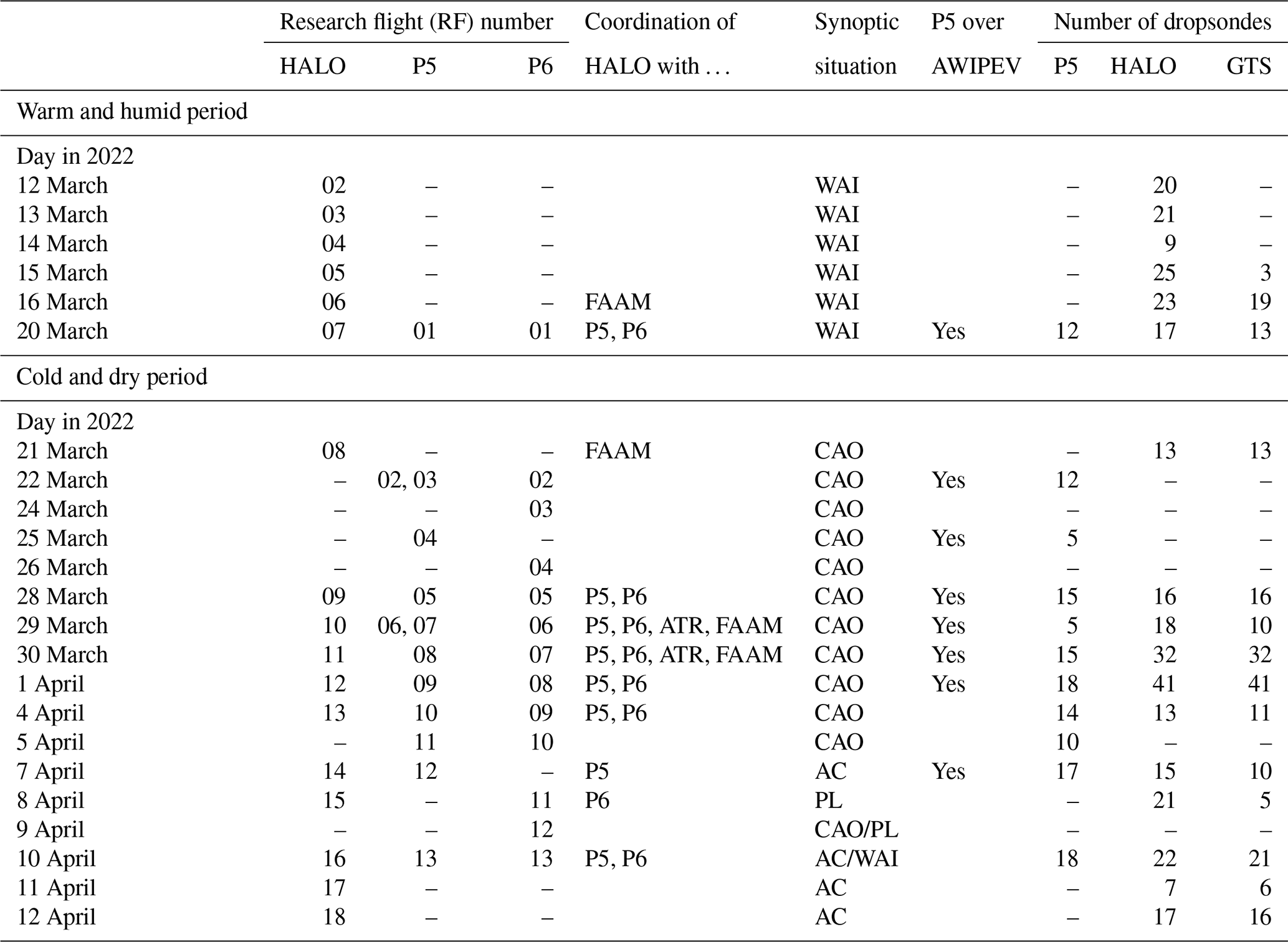
HALO – a Gulfstream G550 – has sufficient range and endurance (up to 9000 km and 10 h) for quasi-Lagrangian air mass observations. HALO is capable of lifting up to 3 t of state-of-the-art meteorological and remote-sensing instruments up to 15 km altitude to observe the complete vertical tropospheric air mass column, including water vapor, aerosol particles, clouds, precipitation, and surface properties. HALO was equipped with a unique remote-sensing payload that has matured in several campaigns in the past (Stevens et al., 2019; Konow et al., 2021). The instrumentation includes a 26-channel microwave radiometer; a 35 GHz Doppler radar; aerosol and water vapor lidar; spectral and broadband solar and thermal infrared radiation sensors, which are upward- and downward-looking; imaging and polarization camera spectrometers in the solar and thermal infrared spectral ranges; and dropsondes. HALO was operated from Kiruna between 7 March and 12 April 2022. In total, 17 research flights (RFs) were conducted (RF02–RF18) with a total flight time of 147 h (Fig. 1a). In total, 330 dropsondes were released from HALO (Table 1).

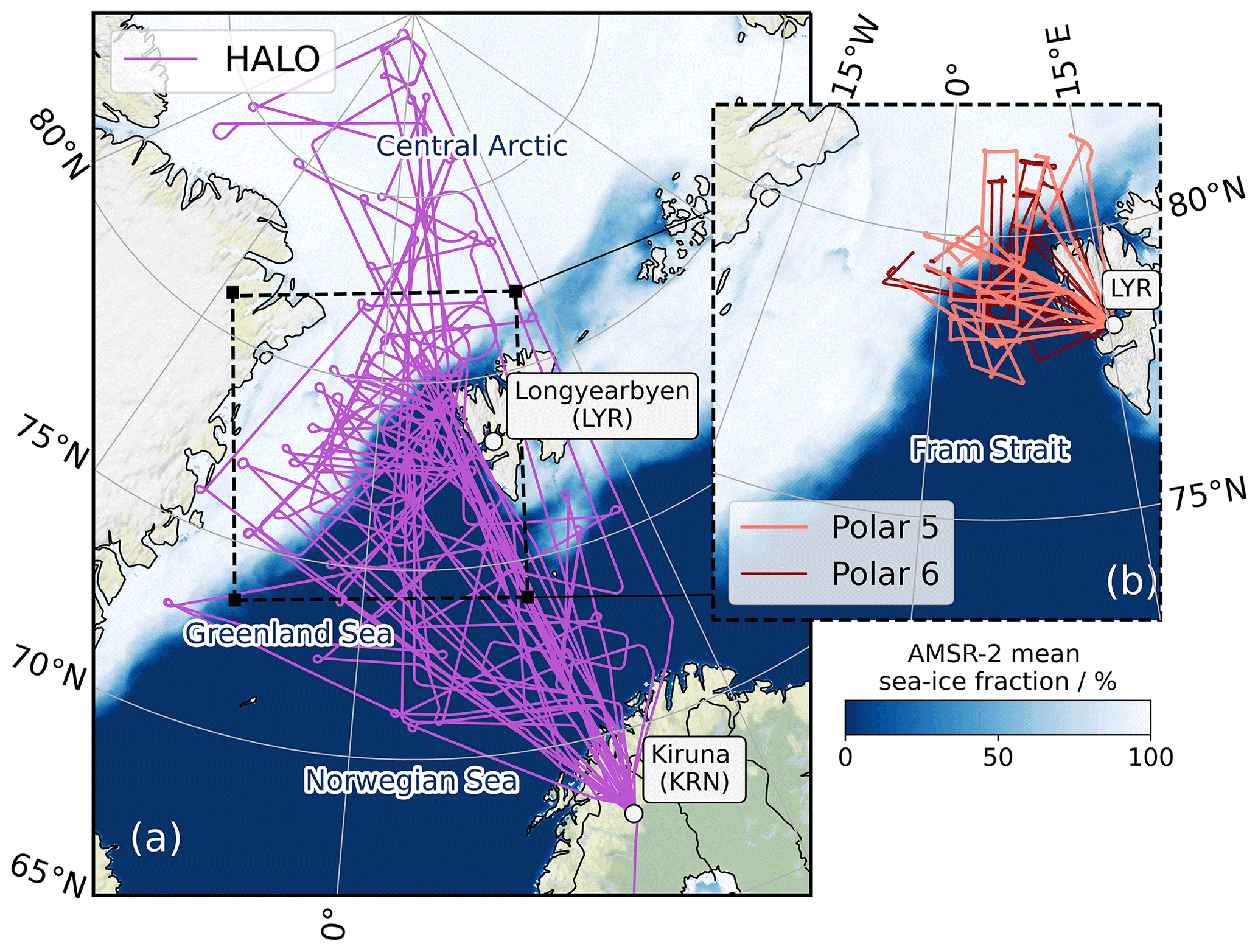
Figure 1 Flight paths (a) of HALO operating from Kiruna (KRN) and (b) of Polar 5 (P5) and Polar 6 (P6) aircraft based in Longyearbyen (LYR).

The low-flying P5 and P6 (Wesche et al., 2016) aircraft are Basler BT-67 (DC-3) types with a ceiling of up to 6 km and a range of about 2300 km. Each of the two planes can carry a scientific payload with a maximum weight of 1 t. P5 provided active and passive remote-sensing measurements to characterize clouds, precipitation, aerosol particles, trace gases, and surface properties from atop, similar to HALO. The instrumentation of P5 included 94 GHz radar, an aerosol lidar, a passive microwave, and radiation sensors. In addition, P5 carried in situ instrumentation to derive turbulence parameters and energy fluxes (Mech et al., 2019; Schirmacher et al., 2023).

P6 focused on in situ measurements in the lower troposphere below 2–4 km altitude in cloudy and cloud-free conditions. The measurements of P6 aimed to determine radiative and turbulent energy fluxes, as well as to investigate smaller-scale processes. For this purpose, P6 was equipped with in situ probes to measure cloud and precipitation particles (droplets and ice crystals) and cloud residuals, aerosol particles, radiation, chemistry, and trace gas properties. For cloud observations, the P6 aircraft was equipped with a cloud droplet probe (CDP), cloud imaging probe (CIP), 2D stereo probe (2D-S), and precipitation imaging probe (PIP) for cloud particle counting and sizing, along with a polar nephelometer (PN) for measuring scattering properties and phase discrimination (Wendisch and Brenguier, 2013; Kirschler et al., 2023; De La Torre Castro et al., 2023). The total data set of the in situ cloud measurements with P6 below 1.5 km sums up to about 21 h, where about 15.5 h were spent above the open ocean and 3.5 h over sea ice.

The P5 and P6 aircraft followed a carefully designed measurement strategy with vertically stacked, colocated remote-sensing measurements above clouds (P5) and in situ sampling inside clouds at lower altitudes (P6). Experiences with this measurement strategy were collected during the Arctic Cloud Observations Using airborne measurements during polar Day (ACLOUD) campaign performed in 2017 (Wendisch et al., 2019). During HALO–(𝒜𝒞)³, both aircraft performed 13 RFs with 53 (P5) and 63 (P6) flight hours, respectively (Fig. 1b). In total, 141 dropsondes were released during the flights of P5 (Table 1). Some coordinated flights between HALO and the P5 and P6 aircraft including closely vertically colocated flight segments were conducted. In addition, several joint flights of HALO, the ATR, and FAAM planes were realized.

Table 1 Overview of HALO–(𝒜𝒞)³ research flights (RFs), including the RF number and information on the coordination of HALO (High Altitude and Long Range Research Aircraft) with the P5 (Polar 5), P6 (Polar 6), FAAM (Facility for Airborne Atmospheric Measurements), and ATR (Avions de Transport Régional) aircraft. Furthermore, the synoptic situation (warm-air intrusion, WAI, cold-air outbreak, CAO, Arctic cirrus clouds, AC, and polar low, PL) and overpasses of P5 over the AWIPEV research base in Ny-Ålesund are indicated. The number of successfully launched dropsondes is given, together with the number of dropsondes used in the Global Telecommunication System (GTS) data assimilation. The direct transmission to the GTS was set up for HALO only. Therefore, all dropsondes listed here submitted to GTS are from HALO.

3 Lagrangian air mass sampling

3.1 Ideal Lagrangian observations using balloons

True Lagrangian measurements would require instruments that are (i) either embedded in the moving-air parcel and taking in situ data along its transport pathway or (ii) flying at higher altitudes and accompanying the moving-air parcel by remote-sensing observations from above. The most suitable instrument platform for achieving approach (i) would be a balloon drifting with the moving-air parcel and carrying devices continuously recording the air mass transformation along its transport pathway. However, balloon measurements suffer from several inevitable drawbacks (Businger et al., 1996; Johnson et al., 2000; Businger et al., 2006; Roberts et al., 2016). For example, even balloons have some non-zero inertia; thus, they do not serve as a perfect instrument carrier to realize approach (i). Furthermore, due to vertical wind shear, the air parcel trajectories differ with altitude and change height levels along their pathways. Therefore, it becomes a non-trivial task to select an altitude level to follow with the balloon. Also, the mass of the instrumental payload that can be lifted by balloons appears quite limited. These and further shortcomings remain when using a balloon as an instrumental platform carrying out remote-sensing observations from above in approach (ii).

3.2 Quasi-Lagrangian approach applying aircraft and trajectories

Here, we try to avoid most of the drawbacks of balloon-borne air mass observations by following a dedicated measurement strategy termed “quasi-Lagrangian” and applying approach (ii). Instead of relying on the limited payload capacity of balloons, we employ three research aircraft equipped with comprehensive instrumentation that have proven their potential in state-of-the-art atmospheric and Earth surface observations. Naturally, aircraft fly much faster than the relatively slow air masses moving with the respective wind speeds. To mitigate this mismatch, we design sophisticated flight patterns aiming to sample the very same air parcels along their pathways at least twice during the same or consecutive flights. To realize this idea, we utilize air parcel trajectory calculations to project (during the flight planning) or reanalyze (after the campaign) the pathways of the air parcels. In case the air parcel trajectory is crossing the flight path twice, we define this as a quasi-Lagrangian match.

This quasi-Lagrangian technique is exemplified by the sketch presented in Fig. 2 for the case of a WAI. At a time t₁, we observe a vertical air column 1 consisting of vertically stacked air parcels. One such air parcel is indicated as a blue cube in this sketch. A number of height-resolving, remote-sensing instruments aboard the high-flying HALO and P5 and dropsondes released during flight characterize the properties of the air parcels at different altitudes within column 1 at t₁. In addition, we probe selected air parcels with in situ instruments installed on P6. Besides many other quantities, dry potential air temperature (θ), specific humidity (q), air temperature (T), and radar reflectivity (Z) are measured by remote-sensing and in situ instruments.

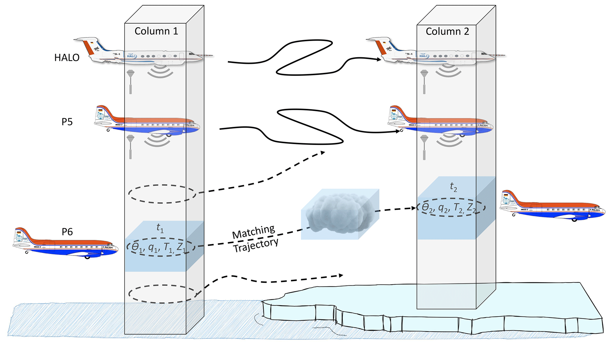
Figure 2 Illustration of the quasi-Lagrangian approach adopted during the HALO–(𝒜𝒞)³ aircraft campaign. At an initial time t₁ and within atmospheric column 1, an air parcel (blue cube) is observed using remote-sensing and in situ instrumentation installed on HALO, P5, and P6. Trajectories are simulated that describe the movement of the air parcels (dashed arrows). If they cross the flight path of the aircraft at a later time, t₂, the air parcel can be sampled a second time within atmospheric column 2. This approach enables observing the changes in the properties of the air parcel (for example, $\mathit{\theta },q,T$, and Z in the time increment (t₂−t₁) along its trajectory).

In the next step, we use forward trajectories (dashed arrows in Fig. 2) to follow the pathways of the individual air parcels of the vertical air column. To calculate the trajectories, we define a horizontal circular area with a radius of 30 km in the center of the air parcel. As an example, we refer to the dashed ellipse within the blue cube of column 1. Starting points are evenly spaced horizontally every 10 km, which results in about 30 regularly distributed points per starting altitude. From the starting points, simulations of the 30 forward-trajectories per starting altitude are performed to project the average movement of the corresponding air parcel (for example, the blue cube in Fig. 2). Subsequently, we follow the same approach for each air parcel within column 1 to project the average movement of the air parcels as a function of altitude.

The vertical geometric thickness of the individual air parcels is assumed to be 5 hPa, which also corresponds to the vertical resolution of the horizontal circular areas. The top of the vertical column is defined as 250 hPa (approximate flight altitude of HALO), which results in a total of 150 (750 hPa divided by 5 hPa) air parcels and horizontal circular start areas for the trajectories. For each of the 150 air parcels in column 1, 4500 trajectories are started (150 parcels × 30 regularly spaced initial points). These trajectories describe the movements of the air parcels in column 1 which were sampled by the three aircraft. Now, the whole procedure is repeated along the entire flight track with a temporal resolution of 1 min. In the case of HALO, the approximate flight time during the HALO–(𝒜𝒞)³ campaign was about 8 h per RF, which means that $\mathrm{4500}\times \mathrm{480}=\mathrm{2.2}\times {\mathrm{10}}^{\mathrm{6}}$ air parcel trajectories have been calculated for each HALO flight during the campaign.

The computation of the forward-trajectories of the air parcels was performed using the Lagrangian analysis tool (LAGRANTO) (Sprenger and Wernli, 2015). During the campaign, the trajectory calculations were based on the Integrated Forecast System (IFS) of the European Centre for Medium-Range Weather Forecasts (ECMWF) wind product. To process the data after the campaign (for this paper), we have applied the Fifth Generation ECMWF Atmospheric Reanalysis (ERA5) (Hersbach et al., 2020). Both methods (IFS- and ERA5-based) have assimilated the dropsonde profile observations of thermodynamic and wind data taken during the flight (Table 1). Trajectories were calculated 60 h forward in time. IFS and ERA5 were retrieved on 137 model levels, which are vertically spaced between the surface and top of atmosphere on a regular 0.25°×0.25° latitude–longitude grid with a 1 h temporal resolution. The improved performance of ERA5 compared to alternative atmospheric reanalyses data has been shown by Graham et al. (2019a, b).

Flight planning to realize quasi-Lagrangian observations required substantial efforts for the mission coordination. To combine flight tracks with the projected trajectories, both were included in our Mission Support tool (Bauer et al., 2022). Then the flight plans were prepared such that there are enhanced chances to meet the air parcel indicated as a blue cube a second time along its trajectory during the flight. This case is illustrated in column 2 of Fig. 2, where the same blue cube within column 1 was actually encountered a second time by the aircraft at time t₂. Such a quasi-Lagrangian match is counted only (i) after at least 60 min of air parcel drift and (ii) if the air parcel trajectory crosses the aircraft track within a 30 km radius. Each quasi-Lagrangian match enables us to compare the air mass properties measured in column 1 (subscript 1) with those measured during the quasi-Lagrangian match in column 2 (subscript 2). Thus, the temporal tendency of a thermodynamic or cloud property ψ (e.g., θ, q, T, and Z) that characterizes the rate of change in a particular air mass property along its trajectory can be quantified using the following equation:

$$\begin{array}{}\text{(1)}& {\displaystyle \frac{\mathrm{\Delta }\mathit{\psi }}{\mathrm{\Delta }t}}={\displaystyle \frac{{\mathit{\psi }}_{\mathrm{2}}-{\mathit{\psi }}_{\mathrm{1}}}{t_{\mathrm{2}}-t_{\mathrm{1}}}}.\end{array}$$

3.3 Example and statistics of matches

We illustrate the quasi-Lagrangian procedure for two HALO research flights (RF03 and RF04) performed within 2 consecutive days (13 and 14 March 2022). In Fig. 3, the notable corridor of increased northward-integrated water vapor transport (IVT) indicates a substantial WAI event. During RF03 on 13 March, the HALO flight path (blue line) was designed to cover the WAI by a horizontal zigzag flight pattern (Fig. 3a–c). HALO took off shortly after 08:00 UTC in Kiruna. The forward trajectories were simulated along the HALO flight path with a 1 min resolution (black lines), with the start times corresponding to the HALO flight time series. Only those trajectories are depicted in Fig. 3a–c that later on, during RF04, matched the HALO flight path a second time. These trajectories evolved until HALO landed in Kiruna around 17:00 UTC. During the night, the trajectories advanced, indicating a continued transport of the humid air masses poleward. HALO took off on the second day (RF04), on 14 March, at around 10:00 UTC and crossed the trajectories that had been initiated on the day before (Fig. 3d–f). Altogether, about 80 000 matches of air parcels (5 hPa vertical and 13–15 km horizontal size) at different altitudes have been obtained during these two consecutive HALO flights.

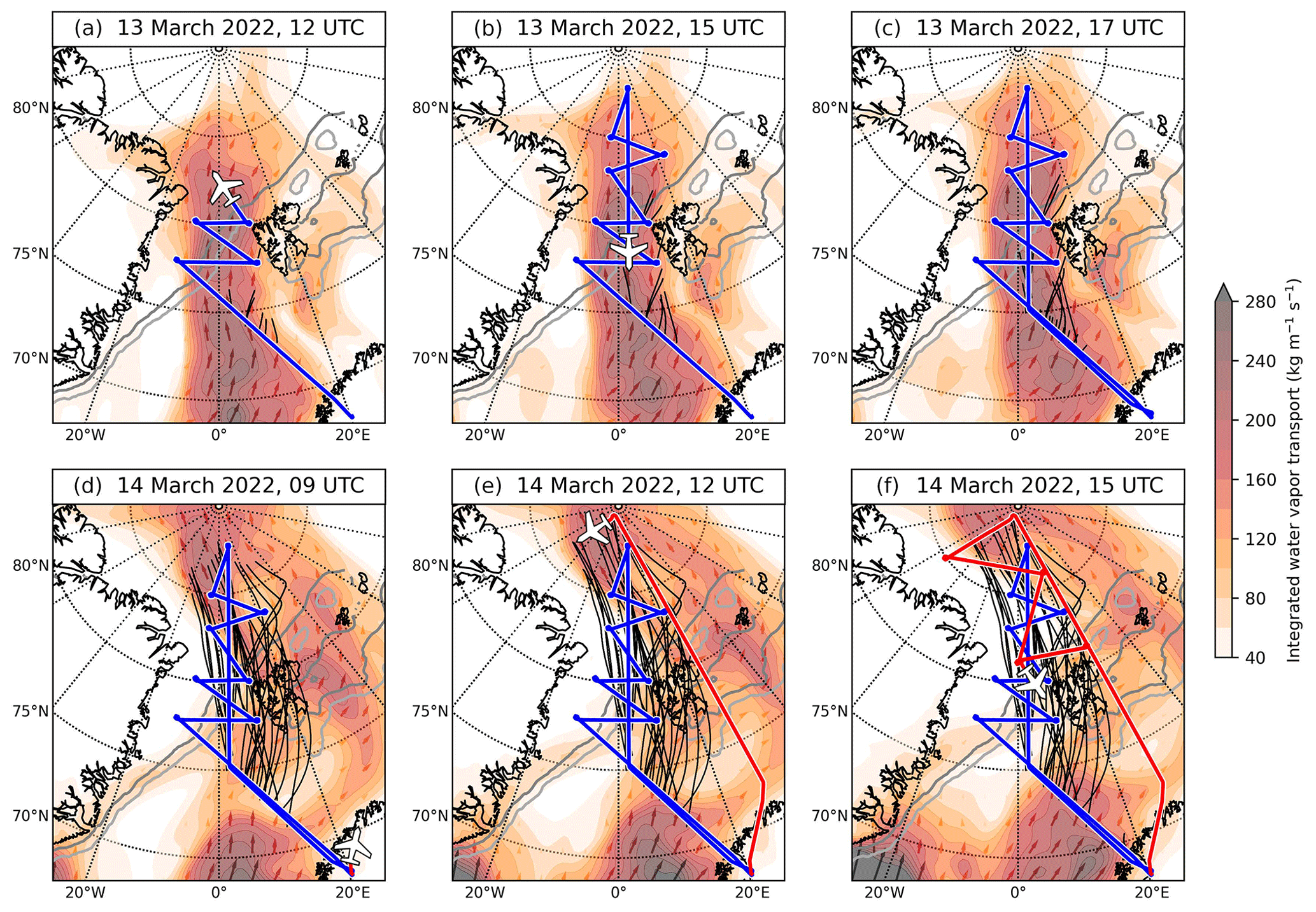
Figure 3 Warm-air intrusion (WAI) on 13 and 14 March 2022. Time series (based on ERA5) of geographic maps, including the integrated water vapor transport (IVT; in red colors, with the length of arrows being proportional to the magnitude of IVT) and the HALO flight tracks on 13 March 2022 (RF03; blue line) and 14 March 2022 (RF04; red line). Black lines indicate the horizontal projections of the evolving matching trajectories.

The procedure described above was applied to all cases when two HALO flights took place on consecutive days. This included not only WAIs or atmospheric rivers 250 (ARs) but also CAOs, Arctic cirrus clouds (AC), and polar low (PL) cases (Walbröl et al., 2024). The respective statistics of the number of quasi-Lagrangian matches are given in Fig. 4a. Numerous cases have been identified where individual air parcels sampled on day 1 have been encountered a second time on day 2. In a similar way, individual flights performed during a single day were analyzed (Fig. 4b). In these cases, matches between different flight sections along the individual flight were identified. Overall, the number of matches in both scenarios (two flights on consecutive days; one flight during 1 d) is more than sufficient for a statistical evaluation, scientific analysis, and discussion. This data set of quasi-Lagrangian matches provides an unprecedented quantity of possibilities for observing and studying atmospheric air mass transformations.

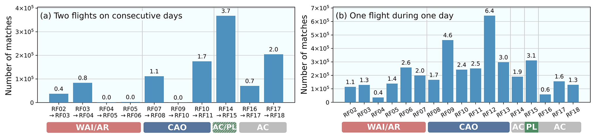
Figure 4 Number of matches for the two scenarios. (a) Two flights on consecutive days and (b) one flight during 1 d. The analysis includes moist- and warm-air intrusions (WAIs), atmospheric rivers (ARs), marine cold-air outbreaks (CAOs), Arctic cirrus clouds (AC), and polar low (PL) cases.

4 Initial results and ongoing analysis

In this section, we provide the first results obtained from the measurements conducted during the HALO–(𝒜𝒞)³ aircraft campaign with respect to air mass transformations (thermodynamic tendencies) quantified during CAOs and WAIs, Arctic cloud evolution during CAOs, and the moisture budget during an example WAI, as well as some characteristic properties of Arctic clouds and aerosol particles. Furthermore, we discuss a proof of concept to measure mesoscale divergence and subsidence in the Arctic.

4.1 Air mass transformations during CAOs and WAIs

4.1.1 Thermodynamic tendencies

To derive the tendencies of thermodynamic properties of the moving-air parcels, such as dry potential air temperature (θ), specific humidity (q), and air temperature (T), we apply Eq. (1) with $\mathit{\psi }=\mathit{\theta },q,z,T$. Corresponding results are depicted in Fig. 5, which illustrates the number of occurrence (counts and color bar) of the temporal tendencies $\mathrm{\Delta }\mathit{\theta }/\mathrm{\Delta }t$, $\mathrm{\Delta }q/\mathrm{\Delta }t$, and $\mathrm{\Delta }T/\mathrm{\Delta }t$ as a function of altitude. In addition, the vertical displacement of the air parcels along its trajectory between t₁ and t₂ is plotted as $\mathrm{\Delta }z/\mathrm{\Delta }t$. The results for the CAO cases (Fig. 5a–d) are derived for trajectories from the north to south; therefore, in general, warming and moistening tendencies at low levels were obtained due to heat and moisture surface fluxes increasing from sea ice to open ocean. The WAI tendencies (Fig. 5e–h) concern the opposite sense, i.e., from south to north.

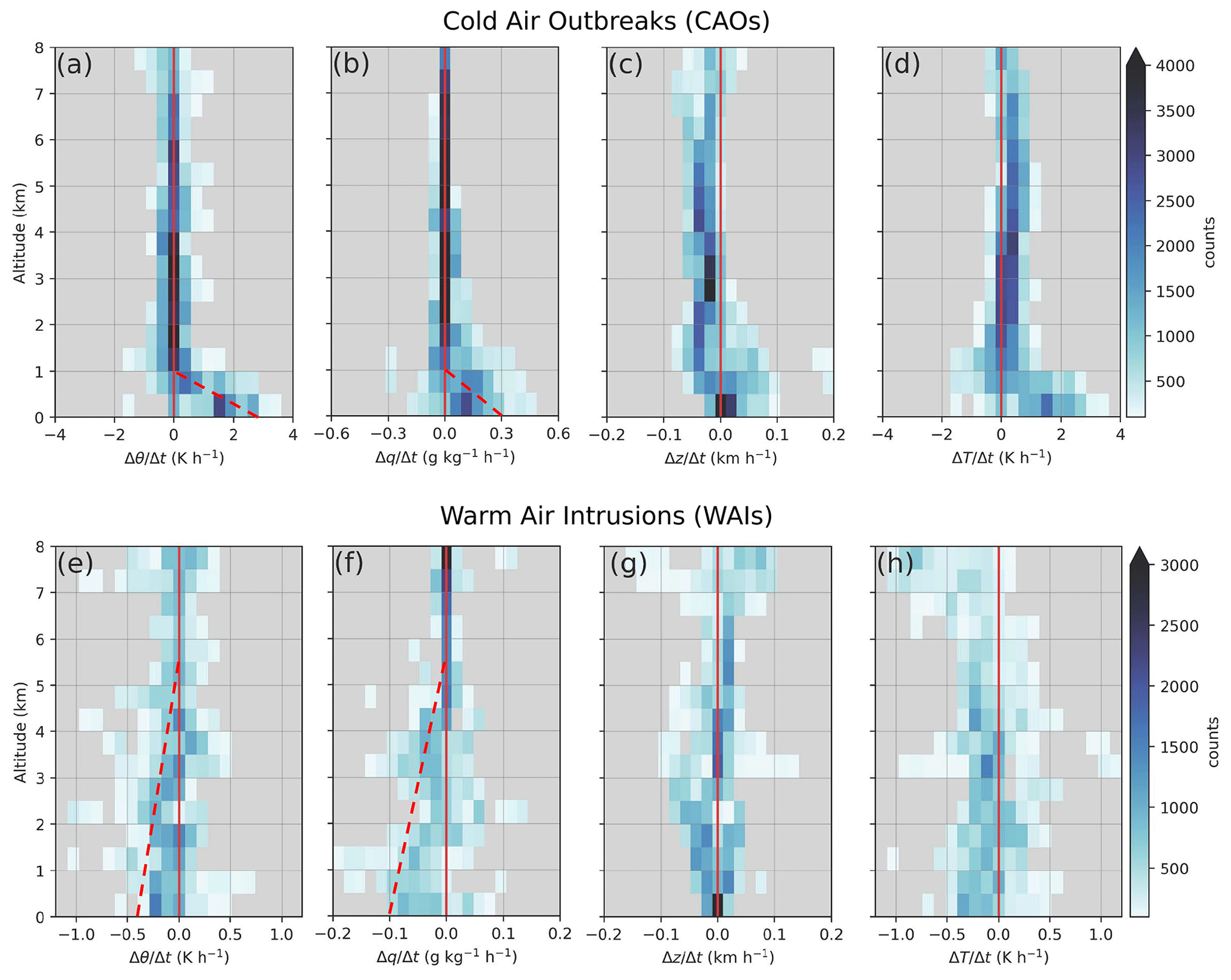
Figure 5 Vertical profiles of the number of occurrences (counts) of temporal tendencies of (a) dry potential air temperature (diabatic heating/cooling; Δθ/Δt), (b) specific humidity (moistening/drying; Δq/Δt), (c) air parcel ascent/descent (Δz/Δt), and (d) air temperature (ΔT/Δt) for marine cold-air outbreaks (CAOs) sampled with HALO on 20, 21, 28, 29, and 30 March and 1 April 2022. Panels (e) to (h) illustrate the same temporal tendencies for moist- and warm-air intrusions (WAIs) observed with HALO between 12–16 March 2022. Vertical solid red lines indicate abscissa values of zero; tilted dashed red lines in panels (a), (b), (e), and (d) indicate the height range of main air mass modification.

It is important to note that the diabatic heating and moistening presented in Fig. 5a–d merge the quasi-Lagrangian matches over open ocean exclusively (CAOs), whereby all available matches (over open ocean and sea ice) are considered in the tendencies for WAIs. In CAOs, major air mass transformations occur over the open ocean due to intense surface turbulent heat fluxes driven by temperature and humidity gradients, whereas the preconditioning over Arctic sea ice typically involves rates 1 order of magnitude smaller (Papritz and Spengler, 2017; Kirbus et al., 2024). Thus, in this article, we focus only on the CAO processes setting in over the open ocean. On the contrary, during WAIs, intense air mass transformations through turbulent, radiative, and cloud processes can set in over open ocean, the marginal sea ice zone, and the sea ice (Woods and Caballero, 2016; Johansson et al., 2017a; You et al., 2022). Therefore, we do not restrict the analysis of air temperature and moisture changes during WAIs to any surface type.

Instead of the air temperature T, we first investigate the temporal tendency of the dry potential air temperature θ, which is insensitive to dry adiabatic vertical movements of the air parcel during transport. Furthermore, θ is characteristic of a moving air mass and changes only in response to diabatic processes. These include cloud evolution (release or consumption of latent heat), surface influences (such as turbulent and energy fluxes), and radiative processes. Using θ instead of T thus quantifies the influence of processes we are most interested in, namely the cloud and surface effects.

For the CAO cases, within the layer between the surface and about 1 km altitude, a surface-driven diabatic heating between 1–3 K h⁻¹ (Fig. 5a) and a moistening between 0.05–0.3 g kg⁻¹ h⁻¹ (Fig. 5b) are observed. Air parcel trajectories are descending throughout most of the vertical column with a wider spread of upward and downward motion in the atmospheric boundary layer (ABL) (Fig. 5c). For the WAI observations, a weak diabatic cooling of up to 0.4 K h⁻¹ (Fig. 5e), and a moisture loss of up to 0.1 g kg⁻¹ h⁻¹ (Fig. 5f) are observed, both reaching from the surface to heights to about 5.5 km. For a specific intense CAO (RF12; 1 April 2022, not shown here), Kirbus et al. (2024) derived a maximum diabatic heating larger than 6 K h⁻¹ close to the ocean surface just downwind of the MIZ. Values of moisture uptake of more than 0.3 g kg⁻¹ h⁻¹ were observed in this study from Kirbus et al. (2024).

For the CAOs, slight subsidence of the air parcels during transport is derived (Fig. 5c). If air temperature tendencies are evaluated instead of dry potential air temperature θ, adiabatic warming effects due to subsidence for the CAO cases become apparent throughout the entire vertical column up to 8 km altitude (Fig. 5d), whereas no distinct adiabatic warming is obvious from Fig. 5a. No clear ascent/descent trends in the air parcels are obvious from Fig. 5g.

Similar to Fig. 5, the cloud reflectivity Z measured by radar on HALO was used to follow the cloud evolution during CAOs and WAIs (not shown). In the case of CAOs, clouds evolve mainly in lower altitudes (below 3 km). In the case of WAI, cloud dissipation dominates mostly below 6 km altitude.

4.1.2 Development of cloud properties during CAOs

First, we investigated how the preconditions over sea ice influence the crucial initial cloud formation using targeted research flights by P5, which statistically sampled the developing roll convection just behind the MIZ (80 %–100 % sea ice concentration). Contrary to previous aircraft studies that followed the air mass downstream along developing cloud streets, the P5 flew multiple legs orthogonal to them. In this way, the roll convection forming the cloud streets could be identified from radar profiles and characterized statistically with respect to their macrophysical and microphysical cloud properties using multiple instruments (Schirmacher et al., 2024). Because air mass transformation is mainly triggered by the exposure of air to open-water surfaces, we used backward trajectories to assign each measurement to its fetch; i.e., the horizontal distance the air mass traveled over open water until reaching P5. Two cases of CAOs of different strengths observed on 1 and 4 April 2022 were analyzed by Schirmacher et al. (2024). The results are summarized briefly here.

The evolution of crucial parameters characterizing the cloud and precipitation development along the two CAOs within the first 170 km is illustrated as a function of the fetch in Fig. 6. Cloud streets form approximately 15 km downwind of the sea ice edge, reaching almost 100 % cloud cover for a fetch of 20 km in both cases. Due to the strong surface fluxes, the ABL grows quickly along the cloud pathway, and the cloud-top height (CTH) increases by about 4 m per kilometer in the strong CAO case (1 April 2022) and only half as much for the weaker CAO (4 April 2022). Both CAO events feature mixed-phase clouds, with the stronger case showing about twice the liquid water path (LWP). Precipitation sets in after a fetch of about 30 km, with a slightly later onset for the weaker event. The combination of remote-sensing data measured with instruments installed on P5 with in situ measurements collected by P6 devices allows the investigation of the ice growth process as reported by Maherndl et al. (2024). For the stronger CAO case, we detect stronger riming, which occurs on a horizontal scale similar to the roll circulation.

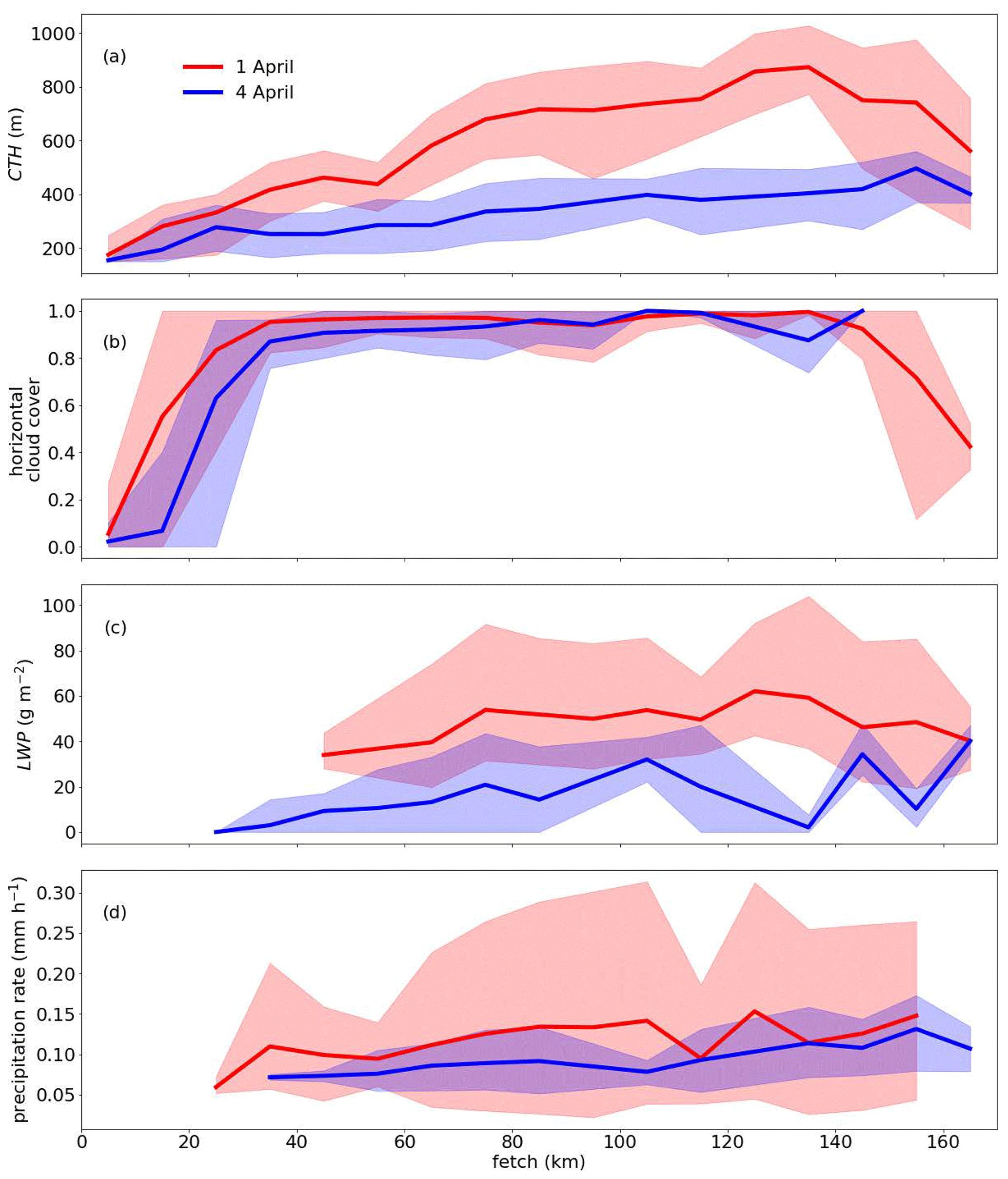
Figure 6 Two cold-air outbreaks (CAOs) – strong on 1 April 2022 and weak on 4 April 2022. Development of macrophysical and microphysical cloud properties as a fetch function on 1 April (red line; strong CAO) and 4 April 2022 (blue line; weak CAO) as measured with instruments installed on P5. (a) Cloud-top height (CTH), (b) horizontal cloud cover per minute measured by the Microwave Radar/radiometer for Arctic Clouds (MiRAC) and Airborne Mobile Aerosol Lidar (AMALi), (c) liquid water path (LWP), and (d) precipitation rate (P) at 150 m height. The shaded areas indicate the 5 % and 95 % quantiles of the distributions as a function of fetch. Figure adapted from Schirmacher et al. (2024).

To understand how CAOs develop from their initial phase along their way further south, HALO, with its long range, can provide valuable insights. The spectral slope phase index defined by Ehrlich et al. (2008) was used to derive information about cloud thermodynamic phase from the measurements (Fig. 7a). Values of the spectral slope phase index smaller than about 20 indicate pure liquid water, and larger values indicate mixed-phase or ice clouds. A transition from pure liquid water to mixed-phase clouds occurs within the first 2 h after passing the MIZ. In addition to the thermodynamic phase, we have retrieved CTH from the Munich Aerosol Cloud Scanner (specMACS) observations with a stereographic method (Kölling et al., 2019; Volkmer et al., 2024) (Fig. 7b). These data were combined with back-trajectories to calculate the time (instead of fetch) at which the measured air mass traveled above the open ocean after passing the MIZ (abscissa in Fig. 7a–b). For the stronger CAO case, images of spatial CTH and cloud thermodynamic phase were gathered by the spectrometer of the specMACS instrument (Ewald et al., 2016; Weber et al., 2024) west of Svalbard during HALO RF12. Figure 7c–e illustrate three example images of the polarization cameras, showing how the clouds in their initial phase organize in cloud streets and then develop into closed cells with increasing distance to the MIZ. While the initial phase with cloud tops up to 1 km was already captured by P5, the HALO observations show that CTH continues to increase up to 2 km.

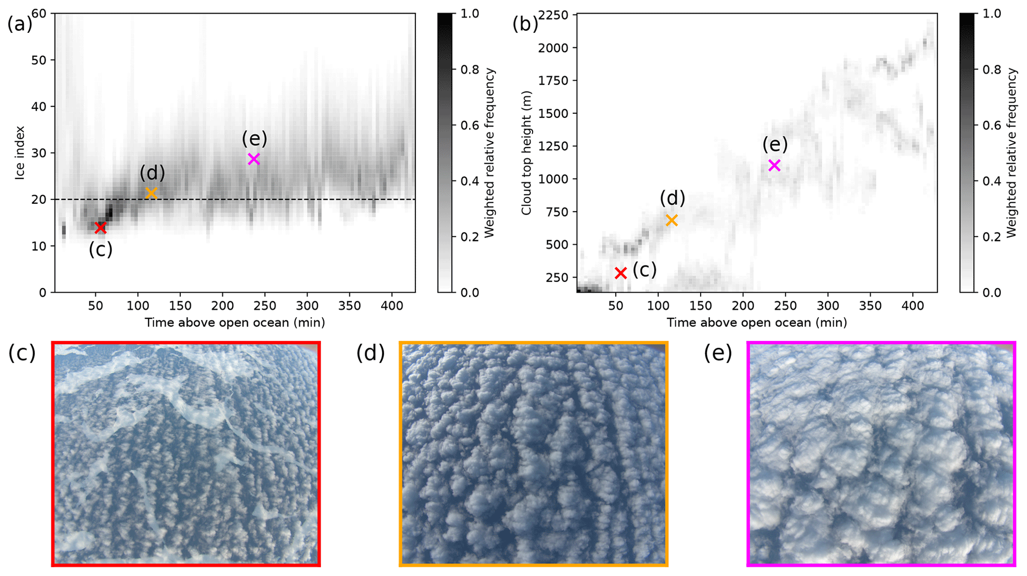
Figure 7 Cold-air outbreak (CAO) on 1 April 2022. (a) Spectral slope phase index (ice index) derived from measurements of the spectrometer of the Munich Aerosol Cloud Scanner (specMACS) as a function of the time the air mass traveled above open ocean. (b) Same as panel (a) but with the cloud-top height (CTH) from a stereographic reconstruction. (c–e) Example RGB (red, green, and blue) images at points indicated by colored crosses in panels (a) and (b).

LWP is a key parameter within the energy and water cycle. Therefore, it is important to understand how the LWP and its spatial distribution develop during CAOs. However, observing LWP is prone to high uncertainties, especially in the Arctic, leading to about a factor of 2 difference in satellite retrievals between passive microwave and solar radiation retrievals (Lohmann and Neubauer, 2018). LWP measurements from P5 and HALO offer opportunities to better constrain satellite observations. For example, Fig. 8a shows the time series of radar reflectivity measured along the flight track of RF08 (Fig. 8b) on 21 March 2022, with high-reaching clouds belonging to the Shapiro–Keyser cyclone over Svalbard (Shapiro and Keyser, 1990). During this flight, HALO probed a CAO in its initial state close to the MIZ flying parallel to the sea ice edge and perpendicular to developing cloud rolls, repeating the pattern with increased distance from the MIZ and finally straight towards Kiruna. To illustrate the quality of different LWP data sets from space and aircraft, we focus on a flight leg for which HALO sampled the transition to cellular convection (Fig. 8c). The cloud radar measurements show a clear rise in CTH for this leg and growing cells southwards. LWP values retrieved from the HALO Microwave Package (HAMP) instrument (Mech et al., 2014) have maximum values around 300 g m⁻² within cells, while close to the sea ice edge, maximum values hardly reach 100 g m⁻² (Fig. 8d). They clearly resolve the individual cells, which is not possible from spaceborne microwave radiometry due to their coarse resolution. Note that the HAMP retrieval only includes the cloud contribution, and thus no enhanced values occur in precipitation. This leg was coordinated with the British FAAM aircraft which focused on in situ measurements of the cloud and sub-cloud layer along this coordinated track and enabled future joint analysis. Due to the time shift between the MODIS (Moderate Resolution Imaging Spectroradiometer) measurement and the HALO flight track, convective cells are shifted between MODIS and HALO measurements. Nevertheless, it becomes clear that MODIS generally shows higher LWP values for these warm-cloud conditions. Our comprehensive measurements from different platforms will be used to further investigate the reasons for this long-standing problem.

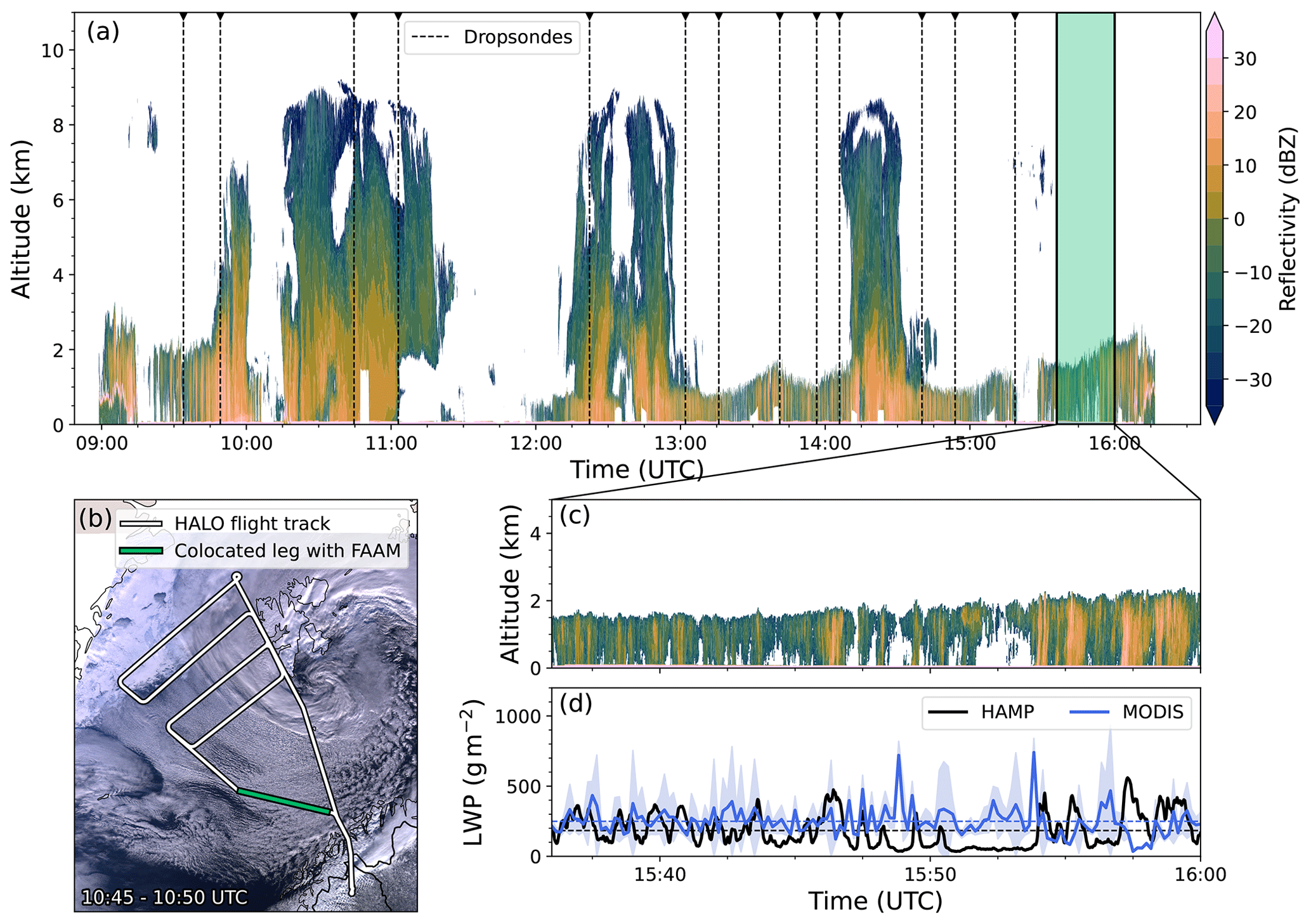
Figure 8 Cold-air outbreak (CAO) on 21 March 2022. (a) Time series of radar reflectivity along the flight track of RF08; the times of dropsonde launches are indicated by vertical dotted black lines. (b) Flight pattern of HALO (white line) and FAAM (green line) during RF08 along the MODIS (Moderate Resolution Imaging Spectroradiometer) overpath (Terra image from 10:45–10:50 UTC; MOD02HKM – Level 1B calibrated radiances). (c) Enlarged view of radar measurements from the last leg which was colocated with FAAM. (d) Time series of the liquid water path (LWP) retrieved from HALO and MODIS (MOD06 – cloud optical properties; two-channel retrieval using band 7 [2.1 µm] and band 6 [1.6 µm]) along the enlarged view of the flight track of RF08. Dashed lines show the temporal mean..

The combination of various remotely sensed measurements with back-trajectory calculations for the targeted CAO flights by P5, P6, and HALO has the strong potential to further investigate CAO cloud development and transitions. Future analysis will include further retrieval development of liquid and ice clouds, e.g., from specMACS, HAMP, and a detailed evaluation of satellite data. Most importantly, the comprehensive measurements provide solid reference data to test high-resolution models that are able to resolve the complex circulation involved in CAOs.

4.1.3 Moisture budget during WAIs

An ultimate test of our understanding of the atmospheric water cycle is provided by checking the ability to close the water budget. For this test, a research flight (RF05 on 15 March 2022) was specifically dedicated to optimally determine the moisture budget components (Eq. 2), including their accuracy for a strong WAI event. These data should serve as a critical test for the respective simulations using the ICON (Icosahedral Nonhydrostatic) model. The governing equation for the moisture budget is given by the local change in the integrated water vapor (IWV) as follows:

$$\begin{array}{}\text{(2)}& \begin{array}{rl}{\displaystyle \frac{\mathrm{d}\mathrm{IWV}}{\mathrm{d}t}}& =-\mathbf{\nabla }\cdot \mathrm{IVT}+E-P+\mathit{ϵ}\\ & =-(\mathrm{ADV}+{\mathrm{DIV}}_{\mathrm{mass}})+E-P+\mathit{ϵ},\end{array}\end{array}$$

with t as the time, E as the evaporation, P as the precipitation rate, IVT as the integrated water vapor transport, and ϵ as the residual. ∇⋅IVT describes the divergence of the IVT; this quantity was derived from the sum of the integral of the horizontal moisture advection (ADV) and the dynamic mass divergence (DIV_mass).

The flight pattern (Fig. 9a) chosen to assess the moisture budget included two legs perpendicular to the flow (thick light green lines; cross-flow) and one internal leg (thick blue line). The moisture flux across the two cross-flow flight legs was estimated from the wind and humidity observations provided by dropsondes (large white triangles). From the difference between exported and imported moisture fluxes determined by the dropsonde observations along the cross-flow flight paths, we estimate that the internal divergence of the moisture flux (∇⋅IVT) was evaluated as one key component of the atmospheric moisture budget. Along the internal leg, measurements of radar, microwave radiometer, and dropsondes were used to derive precipitation rate (P), evaporation (E), integrated water vapor (IWV), and its temporal tendency ($\mathrm{d}\mathrm{IWV}/\mathrm{d}t$). The simulations with ICON were performed in the domain enclosed by the dashed red line in Fig. 9a with a horizontal resolution of 2.4 km.

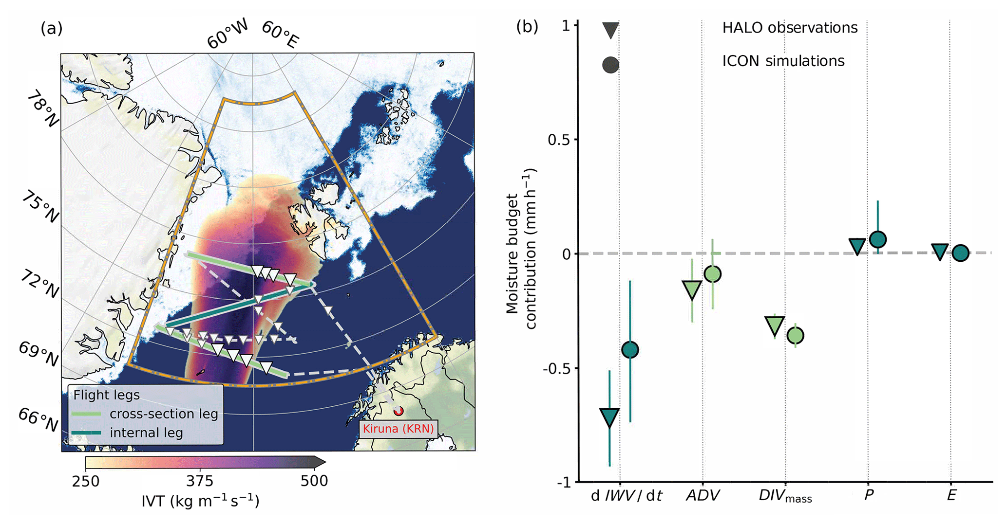
Figure 9 Warm-air intrusion (WAI) on 15 March 2022. (a) HALO flight pattern (dashed gray lines and thick colored lines) and ICON (Icosahedral Nonhydrostatic) model domain (framed by the dashed orange line) for the WAI sampled during RF05. Along the two cross-flow flight sections (thick light green lines), dropsonde observations are indicated by large triangles, whereas small triangles represent the dropsonde releases during the remaining flight sections. The internal leg is indicated by the solid blue line. For the ICON domain, simulated integrated water vapor transport (IVT) values are illustrated in red. (b) For the eastern part of the flight pattern, the moisture budget components from the HALO observations (triangles) are compared to those simulated by ICON (circles) with respect to their contribution to the moisture budget (in mm h⁻¹). Moisture advection (ADV), mass divergence (DIV_mass), precipitation rate (P), evaporation (E), integrated water vapor (IWV), and its temporal tendency ($\mathrm{d}\mathrm{IWV}/\mathrm{d}t$) are compared. Vertical lines indicate the uncertainties for each component.

Figure 9b compares the moisture budget components derived from the HALO observations (full triangles) and ICON simulations (full dots) along the HALO track. The ICON-based and observational estimates agree reasonably well in the quantification of moisture tendency due to mass convergence and surface evaporation, while there are discrepancies regarding the temporal tendency of water vapor. A potential explanation might be the substantial dissipation of the WAI during the flight. Future work will focus on understanding the causes of these discrepancies, closing the moisture budget in the observations, and identifying the major processes for the correct representation of WAIs in models. Here we will exploit RF02, RF03, RF04, and RF06, where meteorological conditions and the flight pattern of HALO are well suited for the estimation of the local moisture tendency and directly compare it with the ICON simulations.

4.2 Arctic clouds

4.2.1 Low-level clouds: thermodynamic-phase distribution

In addition to the spectral slope phase index derived from remote-sensing measurements (Fig. 7a), we have determined the thermodynamic phase of the clouds from in situ measured particle size distribution data in the size range from 2.8 µm to 6.4 mm (Moser et al., 2023). The resulting fractions of ice, mixed-phase clouds, and liquid water clouds are shown as a function of altitude in Fig. 10 and classified into cloud measurements over open ocean and sea ice. Due to the decrease in the temperature with altitude, the fraction of ice clouds over open ocean increases with altitude for altitudes larger than about 500 m. Over sea ice, the ABL shows a high fraction of pure ice and liquid water. In contrast, the cloud characteristics over the open ocean are more variable in height, as mixed-phase and pure liquid water clouds are detected over the whole altitude range.

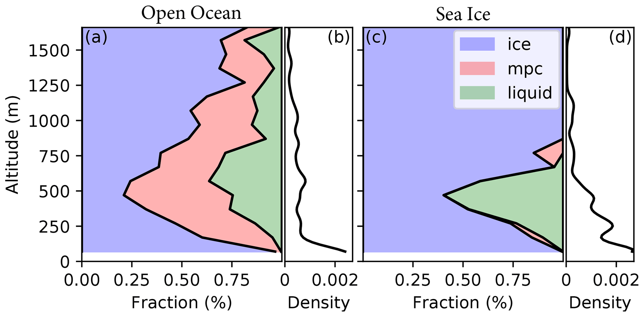
Figure 10 Fraction of detected cloud particle types resolved by altitude. Cloud types (ice is for ice clouds; mpc is for mixed-phase clouds; liquid is for liquid clouds) shown for (a) clouds over the open ocean and (c) clouds over sea ice. Panels (b) and (d) show the distribution of measurements in altitude. Thermodynamic-phase classification was performed according to the algorithm presented by Moser et al. (2023).

These results are obtained from cloud measurements conducted in different meteorological conditions, including CAOs, convergence lines, and polar lows. Future studies will evaluate microphysical properties, including the total number concentration and particle effective diameter of the cloud droplets, as well as the cloud water content. These data will be investigated and discussed in relation to the prevailing synoptic conditions. The results of further statistical thermodynamic and microphysical analyses of low-level Arctic cloud measurements obtained during HALO–(𝒜𝒞)³ will be compared with previous data acquired in the past similar seasons and synoptic situations. Furthermore, the method to detect the thermodynamic phase in Arctic mixed-phase clouds with in situ particle measurements as described in Moser et al. (2023) will be used to validate existing remote-sensing algorithms, such as that of Shupe et al. (2008).

To understand the conditions and feedback mechanisms that maintain the persistence of the inherently unstable mixture of super-cooled liquid water cloud droplets and ice crystals of mixed-phase clouds, a three-dimensional characterization of the thermodynamic-phase partitioning in the clouds is required. For this purpose, the radar–lidar retrieval framework VarCloud was used to derive ice cloud microphysical properties of mixed-phase clouds (Aubry et al., 2024). An example of the simultaneous retrieval of cloud ice and liquid water microphysical properties is given in Fig. 11, which shows the cloud particle (liquid water droplets and ice crystals) effective radius obtained from combined radar–lidar measurements collected during the HALO RF06 on 16 March 2022. The plot shows the cloud cross section within a decaying WAI. On top of the leading marine stratocumulus deck (around 10:30 UTC) and embedded in the trailing ice cloud layer (between 10:15 and 10:20 UTC), the combination of strong lidar with unremarkable cloud radar returns indicates the presence of layers of super-cooled water. These two regions with embedded super-cooled liquid water layers and liquid water-topped ice clouds represent two distinct types of super-cooled liquid water. While the long-lived nature of the latter is well understood, the presence of super-cooled layers embedded within deep-ice clouds requires further investigations that are planned for future work.

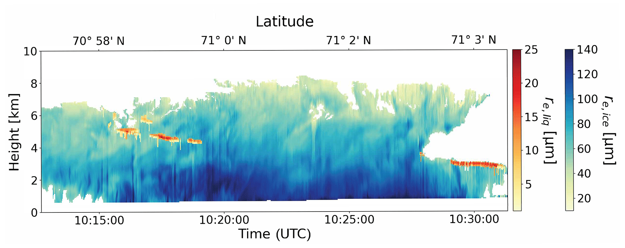
Figure 11 Simultaneous retrievals of effective radius of cloud ice crystals (r_e,ice) and liquid water droplets (r_e,liq) using radar–lidar measurements from the HALO research flight RF06 performed on 16 March 2022.

4.2.2 Cirrus clouds: impact of surface properties and water vapor

The highly reflecting sea ice surface modifies the radiative effects of clouds in general in both the solar and thermal infrared spectral ranges (Stapf et al., 2020; Becker et al., 2023). Here we focus on the surface impact on cirrus cloud transmissivity and emissivity. Compared to the open ocean, the high surface albedo and low surface skin temperature of sea ice increase the relevance of surface properties for the cloud radiative effects. Figure 12a shows the brightness temperature field measured by the VELOX (Video airbornE Longwave Observations within siX channels) instrument (Schäfer et al., 2022) in a broadband wavelength channel ranging from 7.7 to 12.0 µm. For comparison, the time series of the broadband thermal infrared net irradiance measured by the broadband (solar and thermal infrared) irradiance sensor called the Broadband AirCrAft RaDiometer Instrumentation (BACARDI) (Ehrlich et al., 2024) is shown in Fig. 12b. The brightness temperature field shows a tendency to capture lower values during the first half of this flight section (up to 30 km distance), which is caused by an increased ice water path and a reduced emission by the cold cirrus clouds. However, the structure of the sea ice is still imprinted in the measurements (e.g., at 10 and 20 km distance), indicating the high transmissivity of the cirrus clouds.

Figure 12 (a) Two-dimensional brightness temperature field measured by VELOX (Video airbornE Longwave Observations within siX channels) along the flight track in the spectral range of 7.7 to 12 µm. (b) Time series of the thermal infrared (TIR) net irradiance, $F_{\mathrm{net},\mathrm{TIR}}=F_{\mathrm{TIR}}^{\downarrow }-F_{\mathrm{TIR}}^{\uparrow }$, measured by the Broadband AirCrAft RaDiometer Instrumentation (BACARDI) for the same flight section.

Beyond 40 km distance, the cirrus cloud is thinning, and the emitted upward radiation is governed by the surface, which is characterized by a mixture of pack ice and leads characterized by relatively warm open water and young sea ice of a few centimeters in thickness (nilas) for which the surface is also warmer than the surfaces of pack ice and cirrus cloud. Thus, we see an increase in the emitted upward radiance in this region. The thermal infrared net irradiance shows higher values over the cirrus cloud due to a reduced emission compared to the warmer surface. This difference quantifies the top-of-the-atmosphere warming effect of the cirrus cloud, which reaches, in this specific case, up to about 30 W m⁻². However, due to the hemispheric integrating view of BACARDI, the surface variability is not obvious in the broadband irradiance but still might impact the total cirrus cloud radiative effect. Hence, to estimate the total cirrus cloud radiative effect, cirrus cloud and surface inhomogeneities need to be considered.

WAIs lead to an increase in relative humidity and enhance aerosol particle concentrations. Both components can impact the evolution of the cirrus cloud radiative effects. Therefore, it is important to characterize cirrus clouds in the Arctic and their changes due to the increased impact from mid-latitude air masses. Studies on the distribution of relative humidity with respect to ice (RH_i) inside and around Arctic cirrus cloud that formed in WAIs have been performed during HALO–(𝒜𝒞)³ using combined aerosol, cloud, and water vapor measurements from the water vapor differential absorption lidar (Water Vapour Lidar Experiment in Space, WALES) (Wirth et al., 2009), together with temperature information from the model analysis. Particular attention was paid to the vertical distribution of relative humidity with respect to ice (RH_i) within the cirrus clouds, as well as differences with respect to ice supersaturation, giving an estimate of the dominant ice formation processes. From the vertical profiles of cloud properties and RH_i, we found that cirrus clouds formed in air masses transported into the Arctic by WAIs have a larger vertical extent compared to cirrus clouds formed in Arctic air masses (Dekoutsidis et al., 2023).

WAI cirrus clouds are characterized by high ice supersaturation throughout their vertical profile. Figure 13 shows an example of the vertical extent and the RH_i within and around a WAI cirrus cloud measured during RF03 on 13 March 2022. From the backscatter ratio (Fig. 13a), the vertical extent of the cirrus cloud can be derived. A typical backscatter ratio to distinguish the cirrus cloud from cloud-free pixels is around three (Groß et al., 2014; Urbanek et al., 2017). Applying this threshold, it becomes obvious from the example shown in Fig. 13a that for this particular WAI cirrus cloud case, a vertical extent from about 3 km altitude to about 12 km altitude has been obtained. The cirrus cloud is associated with enhanced values of RH_i (Fig. 13b). Values of 140 % and larger are reached, and the majority of data points within the cloud shows supersaturation with respect to ice. This becomes clearly visible when looking at the combined distribution of backscatter ratio and RH_i (Fig. 13c). High values of RH_i within the cloud (backscatter ratio larger than 3) were found, with a peak of the RH_i distribution at about 110 %. Even values exceeding the threshold of homogeneous freezing have been identified inside and around the WAI cirrus cloud. This is in accordance with former findings of Gierens et al. (2020), who used radiosonde measurements to study cirrus clouds in the Arctic.

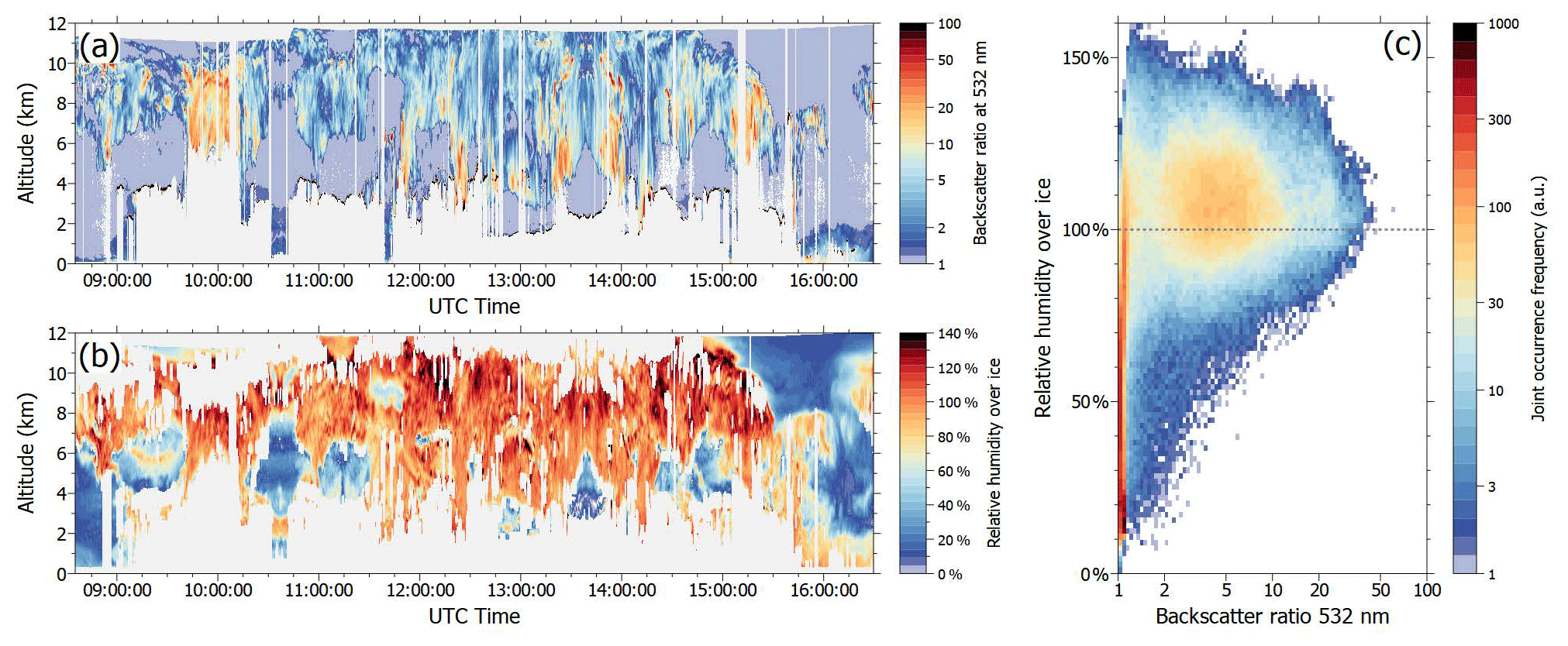
Figure 13 Warm-air intrusion (WAI) on 13 March 2022. Cross section of the (a) backscatter ratio at 532 nm and (b) relative humidity with respect to ice (RH_i) for RF03. Panel (c) shows a histogram of the joint occurrence of the RH_i and backscatter ratio at 532 nm. The relative humidity was calculated from WALES water vapor measurements and the model temperature field.

4.3 Arctic aerosol particles

Sources, abundance, and properties of Arctic aerosol particles in general, and cloud condensation nuclei (CCN) in particular, are not comprehensively monitored. Therefore, aerosol measurements were performed during the HALO–(𝒜𝒞)³ aircraft campaign using data obtained from in situ aerosol instrumentation installed aboard P6. Particles were sampled behind a well-characterized aerosol inlet (Leaitch et al., 2016) and a counterflow virtual impactor (CVI) (Ogren et al., 1985), showing comparable sampling characteristics when both were operated as an aerosol inlet (Ehrlich et al., 2019). Among others, in situ black carbon (BC) measurements were performed by a single particle soot photometer (SP2) installed behind the CVI. Further details on the applied instrumentation are given by Ehrlich et al. (2024).

We have derived typical values of microphysical aerosol properties measured during HALO–(𝒜𝒞)³. Here we present averaged data from the research flights RF08–RF13 of P6 (1–10 April 2022), including periods over open ocean and sea ice. The analysis has shown a median total aerosol particle number concentration N_total of 303 cm⁻³ (interquartile range, IQR = 207–419 cm⁻³; Fig. 14a and d) and a median CCN number concentration N_CCN (measured at 0.1 % supersaturation) of 155 cm⁻³ (IQR = 81–204 cm⁻³; Fig. 14b and e). No obvious change in N_total with altitude became evident up to roughly 1000 m altitude, and only a slight decrease with height can be observed above. Average CCN hygroscopicity (κ measured at 0.1 % supersaturation; Figs. 14c and f) is in the range typical of mostly inorganic aerosol particles mixed with organic material (median values of κ: 0.50; IQR: 0.40–0.68), featuring slightly higher values above 1000 m.

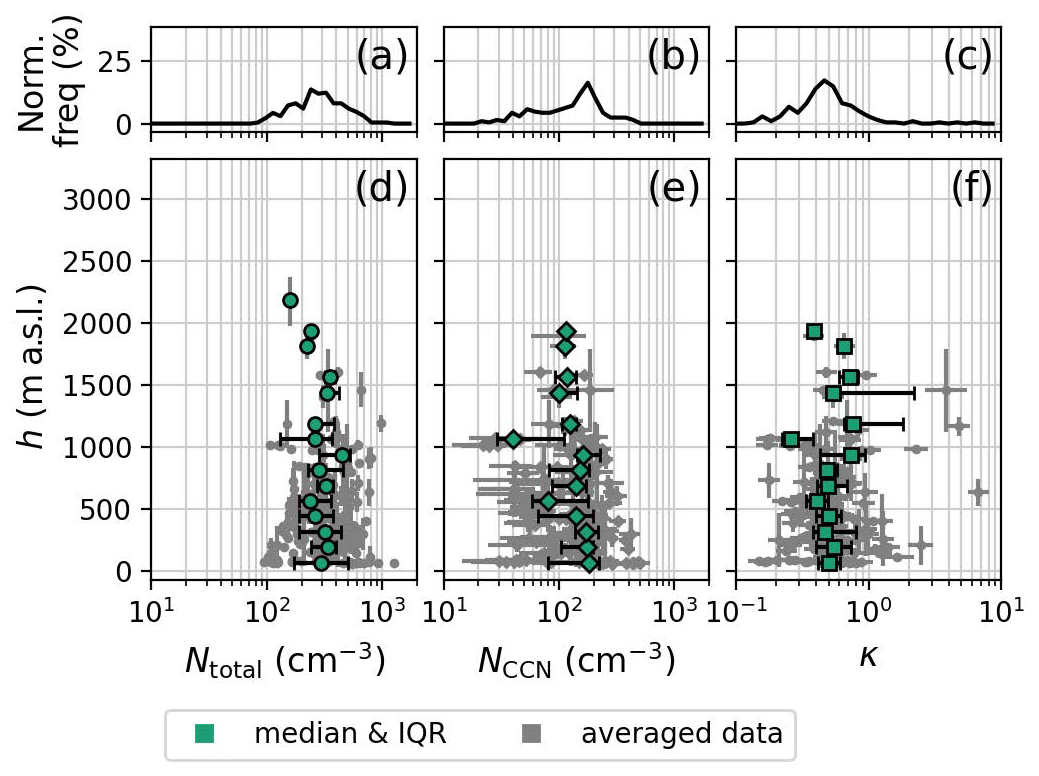
Figure 14 Relative occurrence of the (a) total aerosol particle number concentration N_total, (b) cloud condensation nuclei (CCN) number concentration N_CCN, and (c) CCN hygroscopicity κ. Vertical binned averages of (d) N_total, (e) N_CCN, and (f) κ. P6 research flights RF08 to RF13 are considered.

Furthermore, we have collected and analyzed cloud droplet residuals (CDRs) using the CVI installed aboard P6 (Ehrlich et al., 2019). We have compared the CDR properties (measured inside the clouds) to those of ambient aerosol particles collected in the ABL (below cloud) and in the free troposphere (above cloud). CDR and ambient aerosol particle number size distributions representative of the HALO–(𝒜𝒞)³ conditions in case of low-level clouds probed over open ocean are shown in Fig. 15. Due to the identical shape of the CDR and particle distributions below the cloud level, it is concluded that the cloud is formed and sustained by the activation of ABL particles at the cloud base. A major influence of cloud-forming particles entrained from the free troposphere above the cloud can be excluded since the respective size distribution appears different, which appears similar to the ACLOUD results over open ocean (Wendisch et al., 2019). However, the absence of clouds over sea ice during HALO–(𝒜𝒞)³ did not allow a comparison with ACLOUD results for which the entrainment of cloud-forming particles from the free troposphere was suggested. This analysis will be continued to look for dependencies on the distance to the sea ice edge, the chemical composition of CDR and out of cloud particles, and changing meteorological conditions during the HALO–(𝒜𝒞)³ campaign.

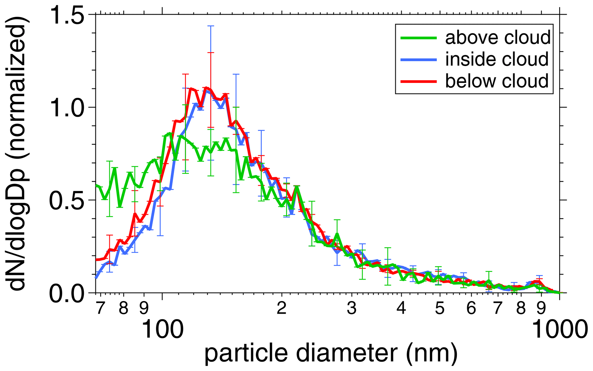
Figure 15 Normalized particle number size distributions of cloud droplet residuals (CDRs; measured inside cloud; blue line) and of ambient aerosol particles (above cloud – green line; below cloud – red line) as measured over open ocean during research flight RF01 with P6 (20 March 2022). The distributions have been normalized with respect to the integrated (total) CDR or ambient particle number concentration.

We also look at the chemical composition of the CDR and ambient particles and their variation with season. For this purpose, we compare observations collected during ACLOUD (late spring and early summer) (Wendisch et al., 2019) with the data available from HALO–(𝒜𝒞)³ (late winter and early spring). The single-particle mass spectrometer ALABAMA (Brands et al., 2011; Clemen et al., 2020) was used to quantify the chemical composition and size of single particles in the size range of 0.23–3 µm (50 % cutoff diameter with respect to detection efficiency). The ALABAMA instrument was connected to the CVI inlet, allowing for sampling of CDR and ambient aerosol particles dependent on the counter-flow settings. Simultaneous measurements of trace gases such as CO, CO₂, and O₃ were used to identify different air mass origins, e.g., to distinguish polluted from non-polluted air masses. The results show a large abundance of particulate amines in ambient air and a dominance of amines in CDR during late spring and early summer (ACLOUD), emphasizing the importance of marine biogenic sources for summertime Arctic cloud processes (Fig. 16). In contrast, amine-containing particles were rarely observed during late winter and early spring (HALO–(𝒜𝒞)³).

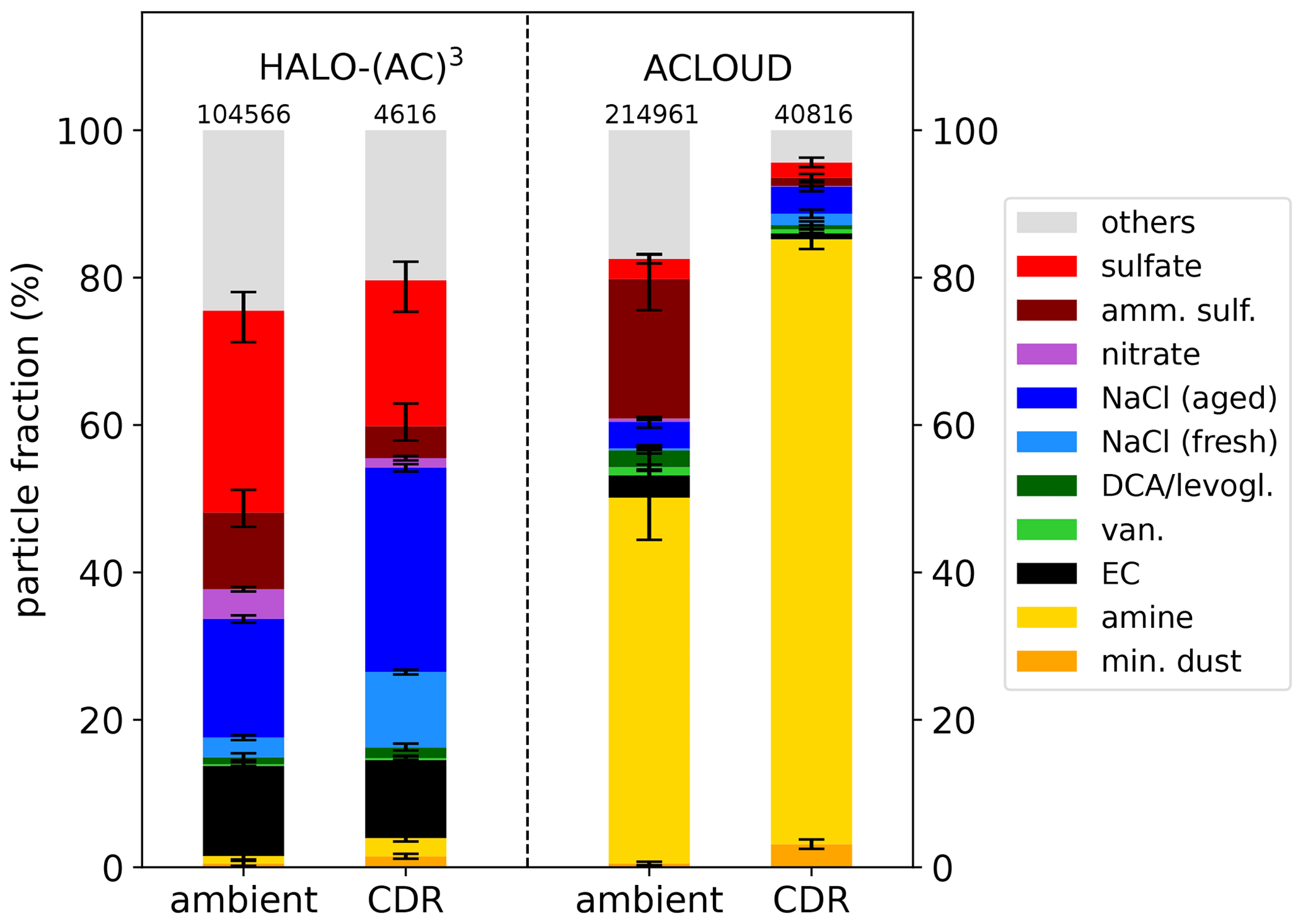
Figure 16 Number fraction of different particle types for ambient particles and cloud droplet residuals (CDRs) during the aircraft missions ACLOUD and HALO–(𝒜𝒞)³ analyzed by the ALABAMA instrument. Note: amm.sulf. is for ammonium sulfate, DCA is for dicarboxylic acids, van. is for vanadium, and EC is for elemental carbon. Particle types are assigned by the dominating peaks in the mass spectra.

Furthermore, the abundance of elemental carbon (EC)-containing particles was proven to be higher during HALO–(𝒜𝒞)³ and accompanied by higher CO mixing ratios than during ACLOUD, indicating the presence of anthropogenic pollution typical of the “Arctic haze” season in spring. These differences between the data obtained during ACLOUD and HALO–(𝒜𝒞)³ reflect the general conclusion that ACLOUD measurements were dominated by WAIs, while CAOs predominated during the HALO–(𝒜𝒞)³ measurement flights of P6. The composition of CDR is similar to that of the particles in ambient air during HALO–(𝒜𝒞)³ but with a higher contribution of fresh and aged sea salt particles to the CDR, while in summer the amine-containing particles dominate the CDR. In future work, a detailed analysis of different air mass situations (WAIs versus CAOs) combined with air mass history analysis (e.g., air mass trajectories) will be performed to investigate the sources of the identified particle types.

4.4 Proof of concept to measure mesoscale divergence and subsidence in the Arctic

ABL cloud transformations at high latitudes play a key role in the Arctic and are partially controlled by large-scale dynamics such as divergence and subsidence. During several research flights of HALO–(𝒜𝒞)³, we have successfully applied a measurement technique using the data from multiple dropsonde releases in circular or quadratic flight patterns to estimate mesoscale properties including divergence, associated subsidence, pressure gradients, and advective tendencies (Paulus et al., 2024). As illustrated in Fig. 17a, HALO RF10 and RF11 probed a weak CAO after applying a quasi-Lagrangian approach. The air mass was sampled at multiple locations during 2 d along its southbound trajectory from the central Arctic into the Fram Strait. The four selected places were determined before take-off, using trajectory estimates based on forecast data. Mesoscale flight patterns surrounding these locations were then incorporated in the HALO flight plan, in principle allowing the calculation of mesoscale gradients across the area (Bony and Stevens, 2019).

The scientific objective of this effort is twofold. First, we aim to test the hypothesis that this novel sampling technique (the sondes) can also reliably yield mesoscale profiles of (thermo-)dynamic circulation properties at high latitudes, in particular in cold, transforming low-level air masses. Various studies have reported encouraging results with this method in marine subtropical areas (George et al., 2021; Bony and Stevens, 2019) and the mid-latitudes (Li et al., 2022). We show that the method works equally well at high latitudes, given the absence of large-scale weak temperature gradients (Charney, 1963; Sobel et al., 2001) and the (partially) associated high transience in synoptic weather. The second objective is to achieve a data set of circulation properties sampled by HALO at mesoscales that is suitable for driving the scientific process models of clouds in CAOs along the trajectory. While CAO cases for large-eddy simulations (LESs) and single-column models (SCMs) have been generated before (de Roode et al., 2019), typically the observational data to realistically constrain the simulation in the upstream areas were lacking. Previous LES studies in the Arctic have shown a strong dependence of Arctic mixed layers on larger-scale forcings, in particular subsidence (Neggers et al., 2019; Dimitrelos et al., 2023), prioritizing the need for such observational data. The HALO–(𝒜𝒞)³ campaign supplies these crucial data for the first time, providing a unique opportunity for exclusively forcing scientific process model experiments for this weather regime with mesoscale data sampled along the trajectory. This has not been achieved before and would represent a step forward in anchoring Arctic process model studies in reality.

Figure 17b–e show the vertical profiles of subsidence as derived from dropsonde data from four “mesoscale circle” flight segments that were flown at selected locations along the 2 d trajectory. The northernmost circle was sampled by HALO RF10, while the southern three circles were flown a day later by RF11. The third HALO circle on the trajectory (RF11 C02) located just south of the sea ice edge was also probed in colocation by the P5 and P6 aircraft, providing additional in situ measurements of clouds, turbulence, radiation, and aerosol properties. We obtain robust profiles of mesoscale subsidence at all four circle sites. For reference, the measured profiles are cross-compared with ERA5 reanalysis data and report a less-than-optimal agreement in general. At circle RF11 C02, the subsidence profile sampled by HALO is reproduced by independent dropsonde data from the P5 aircraft conducted an hour later in the same area and covering only the lowest few kilometers below the P5 aircraft. This agreement, in particular, suggests that the HALO profiles of subsidence are realistic and provides a proof of principle for the applicability of the mesoscale dropsonde technique also at high latitudes.

The encouraging results obtained for this CAO case are fully described by Paulus et al. (2024). They motivate taking the next step and configure LES and SCM experiments for this case that are purely based on HALO measurements. Apart from the divergence and associated subsidence, the data also yield profiles of horizontal pressure gradients (or geostrophic wind) and advective tendencies of temperature, humidity, and momentum. The in situ and independent P5 and P6 data can be used well to evaluate the process model simulations, yielding a complete package for realistic model studies of this CAO. This research is currently in progress.

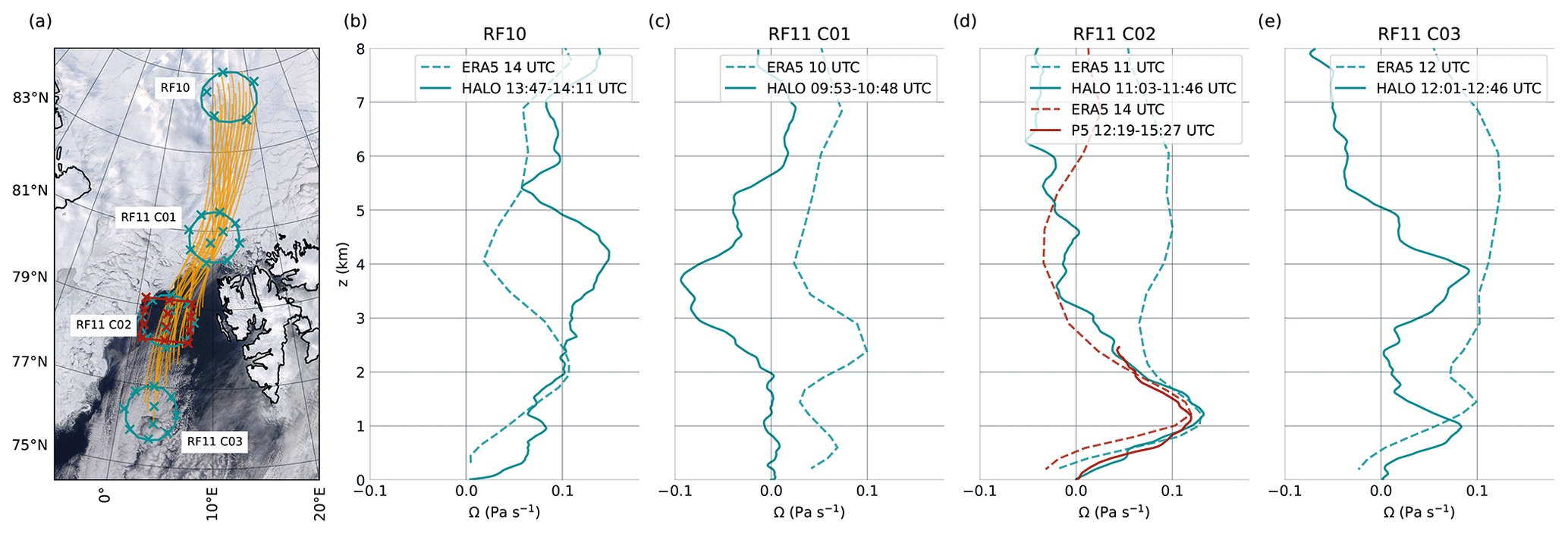
Figure 17 Cold-air outbreak (CAO) on 29 and 30 March 2022. (a) Overview of mesoscale flight patterns flown by HALO (green circles) and P5 (square in a red pattern) sampling a low-level air mass at four locations along its southbound trajectory (yellow lines). Dropsonde launch locations are marked by crosses (green crosses for sondes dropped by HALO; red crosses for sondes dropped by P5). (b–e) Profiles of pressure velocity Ω calculated from dropsonde data (time of first and last dropsonde launch indicated) released from HALO and P5 (solid lines) and ERA5 reanalysis data (dashed lines).

5 Summary and outlook

In this paper, we illustrate the application of a quasi-Lagrangian aircraft measurement approach to observe air mass transformations in the Arctic. The data were collected during the HALO–(𝒜𝒞)³ aircraft campaign that took place between Scandinavia and the North Pole in March and April 2022. We have mainly employed three research aircraft with distinct objectives. The low-flying (mainly within and below clouds) Polar 6 (P6) was equipped with in situ instrumentation to measure aerosol, cloud, and precipitation properties, whereas the higher-flying (mostly above clouds) Polar 5 (P5) aircraft conducted remote-sensing observations of water vapor, aerosol particle, cloud, and precipitation characteristics. The third research aircraft, the High Altitude and Long Range Research Aircraft (HALO), was flying at about 10 km altitude. Whenever possible, HALO was flying closely colocated with P5 and P6. The in situ and remote-sensing payloads of the three aircraft were complemented by numerous dropsonde launches from P5 and HALO.

The focus of the observations was on air mass transformations during moist- and warm-air intrusions (WAIs) and marine cold-air outbreaks (CAOs). The processes during these transformations were observed in a novel quasi-Lagrangian manner, probing the same air parcel twice on its way into or out of the Arctic, either during the same flight (e.g., at its beginning and end) or during two flights on consecutive days. To plan such flights, dedicated air parcel trajectory simulations along the flight paths were employed. A substantial number of matches of the same air parcels was obtained, enabling statistical analysis of the temporal tendencies of potential temperature and moisture during WAIs and CAOs. For the CAO cases, a strong surface-driven diabatic heating between 1–3 K h⁻¹ and a near-surface moistening between 0.05–0.3 g kg⁻¹ h⁻¹ were observed close to the ground below about 1 km. For the WAI observations, a weak diabatic cooling of up to 0.4 K h⁻¹ and a moisture loss of up to 0.1 g kg⁻¹ h⁻¹ were obtained from the ground to about 5.5 km altitude.

We followed the evolution of cloud properties (cloud-top height and cover, liquid water path, precipitation rate, thermodynamic phase, and cloud reflectivity) during CAOs. We have shown that for a strong CAO case, cloud tops are higher, and more liquid water-topped clouds exist. The liquid water path and mean cloud reflectivity measured by radar increase compared to a case of a weaker CAO. In addition, we see how the cloud parameters evolved with distance over the open sea with the atmospheric boundary layer deepening and cloud-top height rising. We observed that for the stronger CAO case, the characteristic features such as the formation of cloud streets and the onset of precipitation occur closer to the sea ice edge.

The moisture budget of a WAI was quantified for the case of a strong WAI. ICON-based and observational estimates of the moisture budget components agree reasonably well for the temporal tendency of moisture due to mass convergence and surface evaporation, while there are remarkable discrepancies regarding the local tendency of water vapor in ICON compared to the HALO data.

The vertical distribution of the thermodynamic phase in low-level Arctic clouds was quantified in a statistical manner using in situ cloud measurements carried out over the open ocean and sea ice. The clouds over sea ice are dominated by the ice phase. In the upper part of the atmospheric boundary layer, liquid clouds are frequently detected. Over sea ice, only a small fraction of the observed clouds is attributed to mixed-phase clouds. In contrast, over the open ocean, the cloud-phase distribution is more variable in height, as mixed-phase clouds and pure liquid clouds are detected over the entire altitude range. Some reasons for the longevity of mixed-phase clouds were discussed using a three-dimensional characterization of the thermodynamic-phase partitioning.

Typical Arctic aerosol characteristics were quantified, and the chemical composition of the aerosol particles was studied. Values of the median total aerosol particle number concentration of 303 cm⁻³ and a median cloud condensation nuclei number concentration at 0.1 % supersaturation of 155 cm⁻³ were derived. No altitude trend in particle numbers is evident up to roughly 1000 m above sea level, but a decreasing tendency was sometimes observed higher up. With regard to the chemical composition of the aerosol particles, a large abundance of particulate amines in ambient air and a dominance of amines in cloud droplet residuals during late spring and early summer is shown, emphasizing the importance of marine biogenic sources for summertime Arctic cloud processes. In contrast, amine-containing particles were rarely observed during late winter and early spring.

It was shown that circular or quadratic flight patterns with sufficiently frequent dropsonde releases provide appropriate data to estimate mesoscale gradients, which can be used to derive subsidence and advective tendencies in the Arctic. These data are highly valuable, for example, for making data available to constrain the initial conditions for large-eddy simulations and avoiding the use of numerical models with a coarser resolution.

Analysis of the results of the HALO–(𝒜𝒞)³ aircraft campaign is ongoing, and the resulting papers will be published in a Special Issue of Atmospheric Chemistry and Physics (ACP) on “HALO–(AC)³ – an airborne campaign to study air mass transformations during warm-air intrusions and cold-air outbreaks”; see (Krämer et al., 2023) and other peer-reviewed scientific journals. Three specific examples of topics that are currently being worked on are given below.

• We will investigate the hypothesis that a secondary circulation acts to spread out moisture from the initial river-like intrusion in the cross-flow direction. This hypothesized circulation consists of uplift in the core of the intrusions, divergence in the upper troposphere above the core, and subsidence of drier air on the flanks of the intrusion. We will investigate the typical structure of the atmospheric moisture field, how it evolves during a WAI, and what the governing drivers of these processes are.

• The particular mode structure of the Arctic radiant energy budget (REB) will be analyzed as a function of altitude, surface type (sea ice or open ocean), cloudy or cloud-free conditions, and thermodynamic properties (temperature lapse rate and horizontal temperature gradient between sea ice and open ocean). The observations will be confronted with model results that often struggle to correctly represent the mode structure of the REB, e.g., due to limitations in the treatment of sub-grid processes including clouds and the sea ice albedo. Therefore, detailed observation–model comparisons are envisioned to identify potential misrepresentations of properties affecting the REB.

• We will integrate measurements obtained during two CAO events observed during HALO–(𝒜𝒞)³ (29 March and 9 April 2022) with data from the literature. The 9 April case was extraordinary for two reasons. First, it was characterized by cloud-free conditions along the entire 180 km north–south flight track across the MIZ to the open ocean, which is very rare and unusual; only at the southernmost position did convective clouds appear. Second, the southernmost position was influenced by the front of a polar low, which was a remnant of a polar low over Fram Strait on the preceding day. We will discuss how the results of our observations on these 2 d fit to earlier measurements.

Evaluating and testing numerical weather and climate models, as well as reanalysis products, using the comprehensive measurements conducted during the HALO–(𝒜𝒞)³ campaign form the second major objective of this project. This goal will further be pursued in future studies using the wealth of available observations from the campaign.