the Creative Commons Attribution 4.0 License.
the Creative Commons Attribution 4.0 License.
 | 22 Jan 2024
Technical note: Emulation of a large-eddy simulator for stratocumulus clouds in a general circulation model
Jukka-Pekka Keskinen
Sami Romakkaniemi
Harri Kokkola
Petri Räisänen
Antti Lipponen
Antti-Ilari Partanen
Jaakko Ahola
Juha Tonttila
Muzaffer Ege Alper
Hannele Korhonen
Tomi Raatikainen
Here we present for the first time a proof of concept for an emulation-based method that uses a large-eddy simulations (LESs) to present sub-grid cloud processes in a general circulation model (GCM). We focus on two key variables affecting the properties of shallow marine clouds: updraft velocity and precipitation formation. The LES is able to describe these processes with high resolution accounting for the realistic variability in cloud properties. We show that the selected emulation method is able to represent the LES outcome with relatively good accuracy and that the updraft velocity and precipitation emulators can be coupled with the GCM practically without increasing the computational costs. We also show that the emulators influence the climate simulated by the GCM but do not consistently improve or worsen the agreement with observations on cloud-related properties, although especially the updraft velocity at cloud base is better captured. A more quantitative evaluation of the emulator impacts against observations would, however, have required model re-tuning, which is a significant task and thus could not be included in this proof-of-concept study. All in all, the approach introduced here is a promising candidate for representing detailed cloud- and aerosol-related sub-grid processes in GCMs. Further development work together with increasing computing capacity can be expected to improve the accuracy and the applicability of the approach in climate simulations.
- Article
(13143 KB) - Full-text XML
- BibTeX
- EndNote


Clouds play a major role in the Earth's climate system through their effects on the hydrological cycle and the radiative balance (Boucher et al., 2013; Rosenfeld et al., 2019). They mainly reflect the incoming shortwave solar radiation and trap outgoing longwave radiation from the relatively warm surface. Cloud radiative effects depend on cloud macro- and microphysical properties like cloud fraction, amount of liquid water and ice, and the size of cloud particles. These properties, in turn, depend on atmospheric thermodynamics and dynamics as well as microphysical processes. Typically, cloud formation is related to updrafts driven by convection, turbulence, or larger-scale weather systems. Precipitation is one of the key cloud microphysical processes influencing cloud dynamics and lifetime.
Accurate simulation of clouds has been a long-standing challenge for general circulation models (GCMs). This is especially true of shallow clouds, in particular marine stratocumuli, which are the focus of this work (Cesana and Del Genio, 2021; Tselioudis et al., 2021). Marine stratocumuli are highly abundant, covering approximately 23 % of the ocean surface, and they strongly influence the climate primarily by reflecting solar radiation (Wood, 2012; Muhlbauer et al., 2014). In spite of their importance, GCMs still struggle to simulate marine stratocumuli realistically. In particular, for decades, most GCMs have underestimated the occurrence of stratocumulus clouds and their impacts on the radiation budget (Siebesma et al., 2004; Teixeira et al., 2011; Lauer and Hamilton, 2013; Jian et al., 2020). The difficulties in representing marine stratocumulus clouds in GCMs arise from two main reasons (e.g., Kawai and Shige, 2020). On one hand, the occurrence and properties of stratocumulus clouds are determined by the interplay of a multitude of physical processes, including turbulence, convection, cloud and precipitation microphysics, and radiative transfer. On the other hand, these issues are exacerbated by the vertical resolution of GCMs that is insufficient to properly resolve boundary layer clouds and especially the inversion layer that controls them (Guo et al., 2019). The clouds are sub-grid-scale features also horizontally. Individual shallow clouds have horizontal dimensions starting from a few tens of meters, while the typical grid spacing in GCMs is 50+ km
The radiative effects of marine stratocumulus are mainly determined by their cloud fraction A and cloud water content qc, also known as cloud macrophysical properties. The recent review paper by Kawai and Shige (2020) separates three basic approaches to parameterize A and qc in GCMs. Either A is diagnostic and qc is prognostic (e.g., Sundqvist et al., 1989), both are prognostic (e.g., Tiedtke, 1993; Wilson et al., 2008), or both are derived diagnostically based on prognostic total water content and liquid-frozen temperature variables (e.g., Smith, 1990; Watanabe et al., 2009). All these approaches require either explicit or implicit assumptions about the sub-grid-scale distribution of total water content. While diagnostic cloud fraction schemes in GCMs typically parameterize A as a function of relative humidity, the parameterizations are sometimes adjusted for stratocumulus clouds by also considering the strength or presence of a temperature inversion (Slingo, 1987; Teixeira and Hogan, 2002; Stevens et al., 2013). A more ambitious approach is the use of unified parameterizations. These include the eddy-diffusivity mass flux (EDMF) approach (Siebesma et al., 2007), which seeks to unify planetary boundary layer (PBL) and shallow convective processes, and the Cloud Layers Unified By Binormals (CLUBB) scheme (Golaz et al., 2002), which attempts to unify cloud microphysics, PBL turbulence, and shallow convection schemes. Suselj et al. (2021) reported significantly improved simulation of subtropical stratocumulus clouds when using the EDMF approach in the NASA GEOS model, while Bogenschutz et al. (2013) reported more realistic simulation of the stratocumulus-to-cumulus transition in the Community Atmosphere Model version 5 (CAM5) in experiments using CLUBB. Similarly, Guo et al. (2014) reported that when using CLUBB with the GFDL atmospheric general circulation model (AM3), the simulations of coastal stratocumulus were significantly improved. Finally, Yamaguchi et al. (2017) developed a methodology named Framework for Improvement by Vertical Enhancement (FIVE), in which selected processes relevant for the simulation of clouds are computed at higher vertical resolution. Lee et al. (2022) showed that FIVE helped to alleviate but still not eliminate the underestimation of subtropical stratocumulus clouds in the Energy Exascale Earth System Model (E3SM).
Aside from cloud macrophysics, cloud radiative effects also depend on cloud microphysical properties. One key parameter is the cloud droplet number concentration (CDNC). CDNC depends on the available aerosol (indirect effect) and the rate of humidity increase, which is typically related to updraft velocity. The importance of aerosol and updraft velocity for droplet concentration has been widely studied. For example, Yoshioka et al. (2019) found the uncertainty in the updraft velocity to be the second most important cause for uncertainty in aerosol radiative forcing, Sullivan et al. (2016) state that input updraft velocity fluctuations can explain as much as 61 % of droplet number variability in GEOS-5, and West et al. (2014) found 0.4 W m−2 uncertainty in the aerosol indirect effect due to different estimates for updrafts in global models. Despite the known importance, most models still rely on a rather simple approach based on the resolved turbulent kinetic energy or eddy diffusivity to parameterize the vertical velocity, which is described by a single grid-scale characteristic value or by a Gaussian distribution of values representing sub-grid variability (Golaz et al., 2011; West et al., 2014; Matsui and Moteki, 2020).
Beyond the direct cloud albedo effect, cloud droplet number concentration also affects the cloud processing and wet removal of aerosol particles and cloud water by precipitation (Matsui and Moteki, 2020). The conversion of cloud water into rainwater and precipitation is based on so-called autoconversion parameterizations (e.g., Seifert and Beheng, 2001; Khairoutdinov and Kogan, 2000; Golaz et al., 2011; Kawai and Shige, 2020). Due to the simplified treatment of both the droplet size distribution and cloud dynamics, global models tend to produce warm precipitation with too little variability in strength (Jing et al., 2019). It is also common for global models that the formation of warm precipitation is too efficient (Suzuki et al., 2015). Related to warm rain formation, attempts have been made to avoid these issues by modifying the autoconversion efficiency either by increasing the cloud droplet threshold size for precipitation formation or simply by scaling the autoconversion strength to account for resolution differences (e.g., Golaz et al., 2011; Mülmenstädt et al., 2020). These modifications and the mathematical dependence of autoconversion rate on CDNC contributes strongly to the spread of modeled aerosol indirect effect (Jing et al., 2019).
In an approach commonly referred to as super-parameterization, the conventional cloud parameterizations within each climate model grid cell or vertical column are replaced with a high-resolution model. For example, cloud-resolving models (CRMs) are well suited for describing a column of a GCM with about 1 km resolution and accounting for additional micro-physical details (Grabowski and Smolarkiewicz, 1999; Stan et al., 2010; Khairoutdinov et al., 2005). CRMs are especially good for simulating cloud systems, and they can cover multiple cloud cycles and types (Khairoutdinov and Randall, 2003). Applying the super-parameterization approach has been shown to significantly improve, e.g., the predictions of surface precipitation compared to conventional GCMs (Tao et al., 2009). However, shallow clouds are still challenging for CRMs, because the CRM resolution is insufficient for resolving even the largest scales of boundary layer turbulence, which has a dominant role for generating the updrafts in shallow clouds. Large-eddy simulators (LESs) are the best tools for such clouds, as these models account for turbulence and they have significantly higher resolution (≲ 100 m) than CRMs have (∼ 1 km). The higher resolution allows them to be based on physics rather than parameterizations. Unfortunately, using a computationally expensive LES as a super-parameterization is currently impossible at least for climate simulations (Grabowski, 2016; Parishani et al., 2017; Jansson et al., 2019).
Computationally efficient machine learning approaches have been used to tackle the super-parameterization problem in climate simulations. In principle, any deterministic model such as LES can be represented by a fast statistical surrogate model called an emulator (Rasp et al., 2018; Glassmeier et al., 2019; Besombes et al., 2021; Conibear et al., 2021). Glassmeier et al. (2019) developed statistical emulators for cloud parameters derived from 159 LES runs with various inputs. Then they used the emulators as advanced interpolation tools to quantify the impacts of aerosol–cloud interactions for a wide range of cloud conditions. Statistical emulators have been used in several occasions to replace the traditional parameterizations and sub-grid-scale models in GCMs (e.g., Reichstein et al., 2019; Yuval and O'Gorman, 2020). The first applications employed neural networks trained using the regular radiation scheme to calculate the longwave radiative budget with reduced computational cost (Cheruy et al., 1996; Chevallier et al., 1998). Similarly, an emulator based on the random forests technique has been used to replace the regular moist convection scheme of a GCM (O'Gorman and Dwyer, 2018). Machine learning approaches have also aimed at developing improved parameterizations based on training data from simulations with a higher model resolution or improved model physics. For example, Han et al. (2020), Wang et al. (2022), and Bretherton et al. (2022) used a deep learning method and training data from a super-parameterized or a kilometer-scale GCM to develop improved parameterizations for moist physics, convection, and radiative fluxes. However, the super-parameterization utilizes a kilometer-scale CRM, so the scheme is best suited for deep convective clouds. In fact, to our knowledge, there are currently no approaches that use LES and machine learning to improve moist physics for shallow clouds in a GCM.
In this study, we present a proof-of-concept for using LES-based emulators to describe processes driving marine stratocumulus cloud properties and life cycle in the global aerosol–chemistry–climate model ECHAM. Our focus is on updraft velocity and warm rain formation, which are among the main sources of uncertainty in the aerosol radiative forcing estimates of current climate models (Donner et al., 2016; Jing et al., 2019; Bougiatioti et al., 2020; Yoshioka et al., 2019). These processes were chosen because, on the one hand, updraft velocity is the dominant factor in hydrometeor number variability (Sullivan et al., 2016) and its emulation is technically relatively straightforward (Ahola et al., 2022). On the other hand, current schemes of precipitation formation in GCMs are quite simplified, producing known biases (Jing et al., 2019; Suzuki et al., 2015). Emulating precipitation formation allows for increased realism for this highly important process, for example, by accounting for the impacts of sub-grid variability in cloud properties. Finally, an important practical aspect is that emulators for updraft speed and rainwater formation can be used in ECHAM without major structural changes in the model parameterizations.
Below we present the emulator development work and compare the obtained results with those from the default version of the same GCM as well as against observations. Our aim is to demonstrate that the new approach results in stable, physically sound GCM simulations, which has been an issue with some previous methods (Yuval and O'Gorman, 2020; Yuval et al., 2021; Brenowitz et al., 2020). We also discuss the lessons learned during the emulator development and present ideas for the way forward.
2.1 Model description
2.1.1 UCLALES-SALSA
The LES model used in this study is UCLALES-SALSA (Tonttila et al., 2017). The model includes both the detailed sectional aerosol and cloud microphysics module SALSA (Kokkola et al., 2018) and the double-moment bulk microphysics parameterization (Seifert and Beheng, 2001; Stevens and Seifert, 2008) used in the original UCLALES (Stevens et al., 1999, 2005). Our previous updraft velocity emulator development work (Ahola et al., 2022) showed that the high computational cost of the SALSA microphysics limited the number of emulator training simulations to a level that was not adequate for practical applications. Therefore, we use simulations from (Ahola et al., 2022) made with the double-moment bulk microphysics. In this model version, the cloud water mixing ratio is diagnosed using the saturation adjustment method. Cloud droplet number concentration is given as an input parameter and is assumed to be the same for all cloudy grid cells. The double-moment warm-rain scheme includes parameterizations for autoconversion, rainwater evaporation, accretion, and sedimentation (Seifert and Beheng, 2001; Stevens and Seifert, 2008). Microphysics is coupled with the LES, which simulates the turbulent atmospheric flows, so that they interact via latent heating. The partitioning of water also influences buoyancy and radiative heating and cooling, which are important drivers of updraft velocity.
2.1.2 ECHAM
The GCM simulations were carried out with the ECHAM (ECHAM6.3-HAM2.3-MOZ1.0) global aerosol–chemistry–climate model (Schultz et al., 2018). It consists of the atmospheric model ECHAM (Stevens et al., 2013), aerosol model HAM (Kokkola et al., 2018; Tegen et al., 2019), and chemistry model MOZ (Schultz et al., 2018). The aerosol model HAM includes two configurations for the aerosol size distribution: modal treatment M7 (Tegen et al., 2019) and the sectional scheme SALSA (Kokkola et al., 2018). From here on, we refer to these model setups as ECHAM-M7 and ECHAM-SALSA. We used the standard ECHAM-M7 setup to generate the input data for the LES training simulations (see Sect. 2.2). However, because our original aim was to include the aerosol impacts by using SALSA microphysics in the LES runs (i.e., UCLALES-SALSA), the emulators were implemented into ECHAM-SALSA. Hence, in the following we focus on ECHAM-SALSA.
Aerosol–cloud interactions in the model are simulated using the two-moment cloud microphysics scheme of Lohmann (2008) and Lohmann and Hoose (2009) with modifications described by Lohmann and Neubauer (2018). In addition, SALSA uses the sectional aerosol size distribution scheme of Abdul‐Razzak and Ghan (2002) instead of the modal setup used in Lohmann and Neubauer (2018). In the default setup of ECHAM, a lower bound of 40 cm−3 for CDNC has been set (Lohmann et al., 1999). This is a common practice in global models to avoid CDNC values which are considered too low (Hoose et al., 2009). However, in ECHAM, this reduces the sensitivity of CDNC to changes in updraft velocity. This is why we reduced the lower bound to the value of 10 cm−3. This allowed for better assessing the impact of the updraft velocity on CDNC but on the other hand resulted in a high aerosol radiative forcing (see Sect. 3.3.4).
Cloud fraction is parameterized as a function of relative humidity (RH), using the assumed humidity distribution function scheme developed by Sundqvist et al. (1989). As detailed in Sect. 3.2.3 in Stevens et al. (2013), the critical relative humidity for cloud formation depends on pressure, and in order to enhance the simulation of stratocumulus clouds, a 100 % cloud fraction is assumed already at RH = 90 % if there is a temperature inversion below 700 hPa. Mixing ratios of cloud liquid water and cloud ice are treated prognostically. The prognostic equations follow the approach described by Lohmann and Roeckner (1996), which accounts for the transport by the adiabatic circulations, exchange terms that convert water from one of the prognostic phases (vapor, liquid, solid) to another, and conversion to large-scale precipitation.
Vertical velocity in the default version of ECHAM is based on a single characteristic vertical velocity, which is calculated as the sum of large-scale and turbulent-kinetic-energy-dependent velocity terms (Lohmann et al., 2007). In the two-moment microphysical module of ECHAM, the rainwater formation rate is calculated using the autoconversion parameterization of Khairoutdinov and Kogan (2000) for each model level. The rate is proportional to the ratio of cloud liquid water content to cloud droplet number concentration.
ECHAM uses a spectral representation of atmospheric dynamics along with a flux-form semi-Lagrangian scheme for tracer transport. In our model configuration, the horizontal resolution was T63, which corresponds to approximately . In the vertical, the model had 47 layers with a terrain-following hybrid vertical coordinate representation (Stevens et al., 2013) with the model top at 0.01 hPa. Sea surface temperatures (SSTs) and sea ice cover were fixed to the monthly mean climatologies provided by the Atmospheric Model Intercomparison Project (AMIP). For simulations with warmer climate, SSTs were increased uniformly by 4 K. Simulations were run for 13 years (1997–2009), and the last 10 years were used in the analysis.
2.2 Emulator development
The main steps of the emulator development are presented in the flowchart in Fig. 1. Steps 1–3, which include the LES and the initial ECHAM-M7 simulations for the selected emulation approach, are obtained from Ahola et al. (2022), so only a brief overview is given here. For this study, we selected the Gaussian process emulation (GPE: O'Hagan (1978) and O’Hagan (2006)) technique, which is suitable for representing the computationally expensive LES. Based on the previous LES runs, we developed emulators for the cloud base updraft velocity and rainwater formation rate. These new emulators were validated using methods similar to those in Ahola et al. (2022).
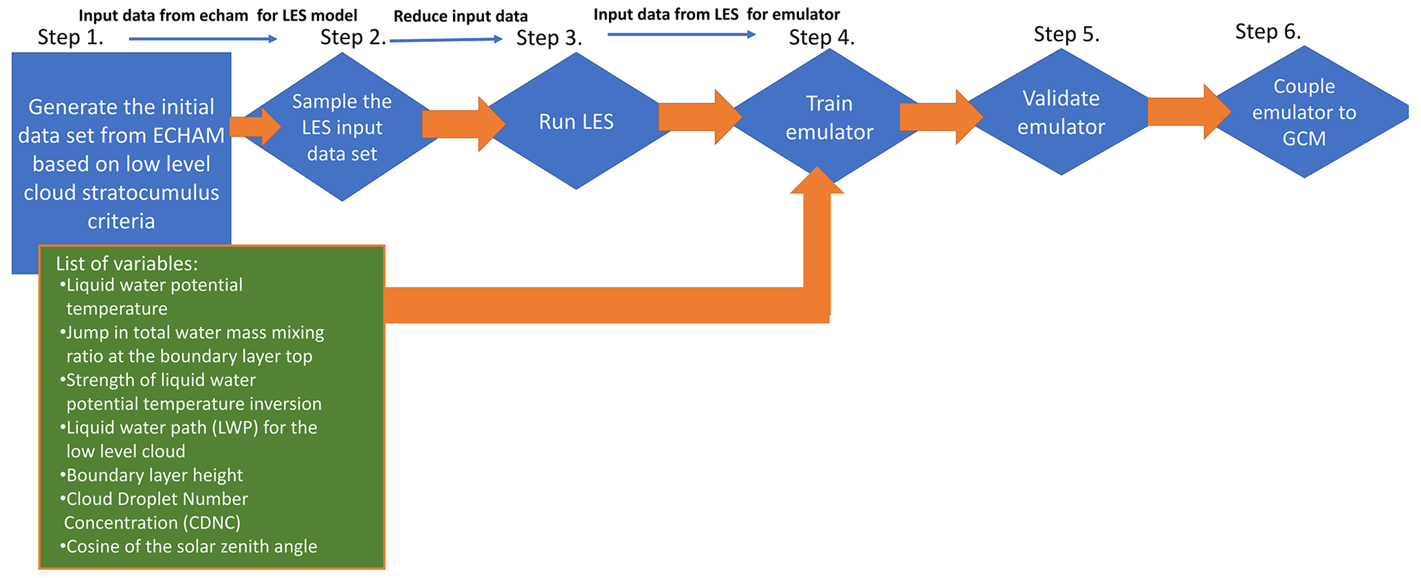
The background information for the emulator training data set was obtained from a year-long ECHAM-M7 simulation. The first step in emulator development was an initial analysis of the GCM (ECHAM-M7), where the conditions for using the emulator and the emulator variables were determined (Ahola et al., 2022). The conditions for using the emulator limited the approach to shallow marine clouds. In practice, this means GCM columns with a warm cloud (at least 90 % liquid) above the open-sea surface (no fog) and below the 700 hPa vertical level (a low cloud). Columns with significant mid- or high-level clouds (more than half of the condensed water located above the low cloud) were excluded as these would have had an impact on the radiative fluxes incident at the top of the low cloud. These conditions for identifying low clouds are fairly relaxed, at least from the meteorological point of view, but they allow applying the emulators to a reasonably high fraction of ECHAM columns, also beyond archetypal stratocumulus regions. It should be pointed out, however, that the emulator is effectively limited to stratus and stratocumulus clouds, as the LES simulations were initialized with a cloud fraction of unity. The reason for this is that the simulation area (10×10 km) and the length of the LES simulations (3.5 h) are insufficient to properly represent mesoscale simulations associated with shallow cumulus clouds (Saffin et al., 2023). Producing an emulator that also better represents shallow cumulus clouds would be an important goal for future work, but it is currently beyond our computational resources.
The emulator input variables are a set of six or seven scalars describing the identified shallow marine cloud columns in a simplified way (Ahola et al., 2022). The additional seventh input variable for the daytime simulations is the (cosine of) solar zenith angle. The variables describing the cloud were derived subject to the assumption of a well-mixed cloud-topped boundary layer, with a constant total water mass mixing ratio and liquid water potential temperature from the sea surface up to the top of the boundary layer. The inversion layer above the boundary layer top is described by the corresponding humidity and temperature jumps. In order to ensure accurate cloud water content, the humidity variable for the emulator is the liquid water path (LWP), but with the above-mentioned assumption it can be related to a certain total water mass mixing ratio. The boundary layer is thus described with three variables: the cloud top height, LWP of the low cloud, and liquid water potential temperature, which is the minimum value in an ECHAM column within the distance of two grid cells from the boundary layer cloud. The humidity and temperature jumps are calculated as the difference between the maximum and minimum values of the total water mass mixing ratio and liquid water potential temperature within the distance of two grid cells from the cloud. The sixth variable is CDNC, which is averaged over cloudy grid cells.
As mentioned above, the initial data set of the emulator input variables was obtained from a year-long ECHAM-M7 simulation with a 1-year spin-up. The conditions above resulted in almost 6×10⁶ ECHAM columns, which are described by the six or seven variables, so the second step in emulator development was to sample a representative subset for the LES runs. For this Ahola et al. (2022) applied the binary space partitioning (BSP; Fuchs et al., 1980) approach. The BSP method uses variable distributions to construct the emulator training data sets so that they well represent the variable space and therefore are beneficial for the emulator. Because nighttime simulations are independent of the solar zenith angle, separate day and night samples were collected. Both of these samples contain 500 cloud cases.
The third step in the emulator development was running the LES simulations. The five meteorological input variables describing the well-mixed cloud-topped boundary layer were used to reconstruct the initial temperature and humidity profiles for the LES runs, again assuming a well-mixed cloud-topped boundary layer. CDNC and solar zenith angle were inputs for the cloud microphysics and daytime radiative transfer calculations, respectively. The other model settings and the simulations are described in Ahola et al. (2022).
Here we used the LES data set from Ahola et al. (2022) for calculating cloud base updraft velocities and rainwater formation rates for the emulator training (step 4). The updraft velocity was calculated as the average of positive (updraft) cloud base vertical velocities from the last hour of each 3.5 h simulation (Romakkaniemi et al., 2009). Three daytime simulations had no clouds during the last hour, so these cases were excluded from the emulator training. The rainwater formation rate is based on domain mean vertical integrals of the removal (below-cloud evaporation and surface precipitation) rates that are multiplied by minus one. We used the removal rates instead of the actual formation (autoconversion and accretion) rates mainly to avoid the impact of spin-up (the first 1.5 h) on the parameterized autoconversion. Namely, autoconversion has the highest rates when the process is switched on after the spin-up. Typically, the rates decreased and reached a steady state within 30 min, but there were a few exceptions with high rates until the end of simulation. Precipitation and below-cloud evaporation depend on the rain droplet size distribution, and its development is limited by the accretion process, so unrealistic rates are much less frequent. Precipitation rates will eventually decrease due to the removal of condensable water. For this reason, the rainwater formation rate was calculated as the average of the three largest values in each LES simulation representing a developed rain drop size distribution.
Separate emulators were trained for each output (updraft velocity and rainwater formation rate) and for daytime and nighttime because the daytime emulators have solar zenith angle as an additional input. In all emulator applications mentioned here we used the GPF Fortran library (https://github.com/ots22/gpf, last access: 4 April 2023) extended for our purpose. In practice, the emulator training means optimizing hyper-parameters of the covariance function (here we added a new covariance function combining squared exponential and linear terms) so that the emulator predictions match with the target outputs (Rasmussen and Williams, 2005). Emulator predictions are based on the hyper-parameters and covariance matrices calculated from the training data set (the LES inputs and the corresponding outputs). We used an offline emulator training approach where these emulator parameters were first saved to a data file, and later the parameters were simply read to the emulator coupled to the GCM (step 6). Practical details about the coupling are given in Sect. 2.3.
To evaluate the emulators' accuracies, we used the leave-one-out cross-validation method (step 5). In this method, one member of the training data set is left out of the training, and a validation emulator is trained using the remaining data. The trained validation emulator is then used to predict the output of the member not used for the training. This process is repeated for each member of the training data set. With this approach, the validation data are independent of the training data and correspond to emulators trained with as complete training data as possible. A large training data set is important in the validation as the emulator performance improves with more training data samples added. Furthermore, in leave-one-out cross-validation, the training data sets of the validation models differ only by one data sample of the training data used to train the final emulator. Therefore, the leave-one-out cross-validation method gives a realistic understanding of the final emulator's accuracy. Emulator validation results are shown in Sect. 3.1.
2.3 Emulator–ECHAM coupling
We have implemented the four different emulators (updraft velocity and rainwater production rate for day and night) in ECHAM-SALSA. All following simulations were made using this model setup, so from now on we drop the suffix SALSA. In addition, we use the term precipitation instead of rainwater production rate, because precipitation in ECHAM is directly related to the rainwater production rate. The daytime versions of the emulators are activated when the cosine of the zenith angle is positive. Otherwise the nighttime versions are used. In all cases, emulation is applied only in columns where the column selection criteria, as defined earlier in Sect. 2.2, are met.
In the default version of ECHAM, the updraft velocity is calculated as the sum of large-scale and turbulent vertical velocity. It is then used in the cloud droplet activation scheme (Abdul-Razzak et al., 1998; Abdul‐Razzak and Ghan, 2002). The coupling of the updraft velocity emulator to ECHAM was straightforward: the original updraft velocities within the cloud layer were simply replaced with the value given by the emulator.
The inclusion of the precipitation emulator was more complicated. As clouds can span several model layers in ECHAM but the emulator provides only a single vertically integrated value for each column, an approach for the distribution of emulated precipitation to model levels was required. In the two-moment microphysical module of ECHAM, the autoconversion rate is calculated using the approach of Khairoutdinov and Kogan (2000) for each model level, which in turn modifies the simulated cloud water mass mixing ratio. In an attempt to preserve the vertical structure of precipitation, we chose to divide the emulated column precipitation to cloudy levels in the same manner. More specifically, the emulated precipitation Pe () for layer i is calculated as
where q is the grid box mean cloud liquid water content (kg kg−1), N is the cloud droplet number concentration (m−3), and index j covers the low cloud. The emulated precipitation is then enforced on each cloudy layer by scaling the terms that make up the precipitation in ECHAM (i.e., autoconversion with droplets inside the layer and accretion with rain drops from above layers). To ensure conservation of water, the maximum amount of precipitation after the application of the precipitation emulator is limited by the available cloud liquid water within the grid box. Here the term cloudy refers to grid boxes in which the liquid water content is at least 0.01 g kg−1.
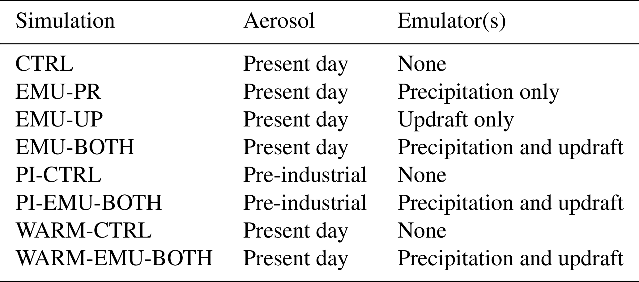
2.4 Experiment design
The emulators implemented to ECHAM were tested in a set of simulations, the results of which were compared against the standard ECHAM setup as well as against observations listed in Sect. 2.5. The eight ECHAM simulations are summarized in Table 1. They consist of four present-day simulations (CTRL, EMU-PR, EMU-UP, and EMU-BOTH), two simulations with pre-industrial aerosol emissions (PI-CTRL and PI-EMU-BOTH), and two simulations with warmer climate (WARM-CTRL and WARM-EMU-BOTH). In the control (CTRL) simulation, the emulators are invoked only for diagnostic purposes, and default parameterizations are used for integrating the model state forward in time. In EMU-BOTH updraft and precipitation emulators are both applied, whereas in EMU-UP only the updraft emulators and in EMU-PR only the precipitation emulators are active. For estimating the aerosol effective radiative forcing (ERF), we conducted the PI-CTRL and PI-EMU-BOTH runs, which are identical to the CTRL and EMU-BOTH runs except that aerosol emissions are from year 1850. ERF is calculated as the difference between the net top-of-atmosphere radiative fluxes in the present-day and pre-industrial runs. The two simulations with warmer climate were made for exploring how the emulators perform in climatic conditions different from the training data set and how they impact the climate sensitivity of the ECHAM model. For this we follow the method by Cess et al. (1990), where the warm climate is produced by increasing the SST uniformly by +4 K.
For the simulations with present-day aerosol emissions, we used the ACCMIP emission data (Lamarque et al., 2010) until the end of year 2004, and after that the emissions come from the representative concentration pathway (RCP) projection RCP4.5 (Van Vuuren et al., 2011). For the pre-industrial simulations, we used the ACCMIP aerosol emission data for the year 1850. Dust, sea salt, and marine dimethylsulfide (DMS) emissions were calculated online based on 10 m wind speed. Dust emissions are based on Tegen et al. (2002) with modifications described by Cheng et al. (2008) and Heinold et al. (2016), sea salt emissions are based on Guelle et al. (2001), and online DMS emissions are according to Kloster et al. (2006).
2.5 Observations
The present-day simulations with and without emulators are compared against observational data sets of surface precipitation and shortwave cloud radiative effect (SW-CRE). The precipitation data set comes from the Global Precipitation Climatology Project (GPCP) (Adler et al., 2012), and for SW-CRE we use the Clouds and the Earth’s Radiant Energy System (CERES) Energy Balanced and Filled (EBAF) top-of-atmosphere (TOA) edition-4.0 data product (Loeb et al., 2018). In addition, we use cloud cover data from Stubenrauch et al. (2013) and LWP data from the Multi-Sensor Advanced Climatology of LWP (Elsaesser et al., 2016). These same observational data sets were used by Neubauer et al. (2019) in their evaluation of the ECHAM6.3-HAM2.3 model. For the comparison, we averaged the model and observational data from year 2000 to 2009.
First we show a brief validation of the emulators by comparing the emulator, LES, and ECHAM predictions for updraft and precipitation. Then we show where and how frequently the emulators are used in ECHAM and how this influences the simulated cloud states. Finally, we show how the emulators influence the simulated climate by examining cloud cover, surface precipitation, shortwave cloud radiative effect, and aerosol effective radiative forcing.
3.1 Emulator evaluation
Figure 2 shows the correlation between standalone emulator predictions and LES outputs (i.e., the truth) for the daytime and nighttime rainwater production rates and updraft velocities. Here the emulator predictions are based on the leave-one-out cross-validation method (see Sect. 2.2). The insets show the corresponding error distributions as histograms. For clarity, the histograms cover a limited range of values, and those exceeding the lower or upper limits are added to the first or last bin, respectively.
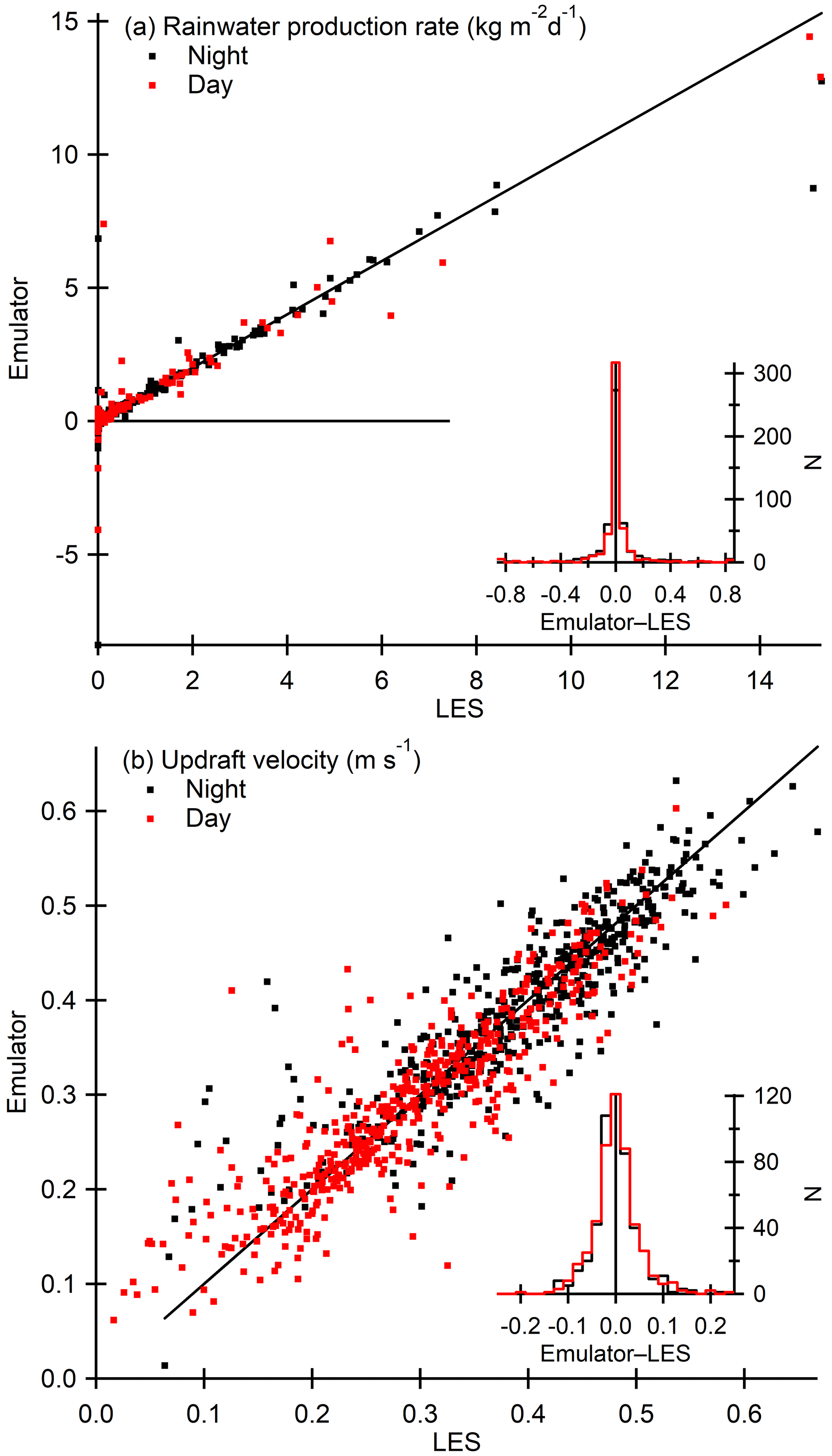
Figure 2Correlation between standalone emulator predictions and LES outputs for nighttime (black markers) and daytime (red markers) rainwater production rates (a) and updraft velocities (b). The insets show the corresponding error distributions as histograms.
Figure 2a shows that most rainwater production rates are close to zero and the larger rates cover a wide range of values from less than 0.1 to well above 10 . The wide range of possible values can explain the few clear outliers (differences exceeding 5 ), but otherwise the emulator is able to reproduce the LES predictions relatively well (95 % of the absolute errors are less than 0.33 ). Pearson’s correlation coefficient, mean error (bias), mean absolute error (MAE), and root mean square error (RMSE) are 0.925, −0.0084, 0.108, and 0.526 , respectively. Figure 2b shows that updraft velocities and their errors are more evenly distributed. Although there are a few outliers where the difference exceeds 0.2 m s−1, 95 % of the absolute errors are still less than 0.1 m s−1. Pearson’s correlation coefficient, bias, MAE, and RMSE are 0.914, 0.0011, 0.033, and 0.047 m s−1, respectively.
Figure 3 shows rainwater production rate and updraft velocity distributions from the LES, ECHAM, and emulators. The four different cases are
-
LES, the original emulator training data calculated from the LES outputs;
-
LES emulator, standalone emulator predictions from the leave-one-out cross-validation shown in Fig. 2;
-
ECHAM, outputs from the default parameterizations collected from the first year (2000) of the control simulation from columns that meet the column selection criteria;
-
ECHAM emulator, outputs from the implemented emulators collected from diagnostic emulator calls for the first year (2000) of the control simulation from columns that meet the column selection criteria.
The updraft velocity distributions from LES and the LES emulators are very similar (Fig. 3b), which means that the emulator reproduces the distribution accurately although individual predictions can be noisy (Fig. 2b). Because rainwater production rates cover several orders of magnitude, the distributions are shown in the logarithmic scale (Fig. 3a). The LES predicts a positive rainwater production rate for any cloud, which explains the high occurrence of practically negligible values lower than 10−3 . Because the emulator predictions include a small noise term, absolute values smaller than 10−3 are being cut out while the values near 10−2 have a higher probability. Because of the noise, the emulator occasionally predicts negative values (see Fig. 2). Negative values are not shown in the logarithmic distribution, but these explain the missing probability density (area below each line). The LES and the emulator distributions agree quite well above 10−2 , where the noise term becomes insignificant.
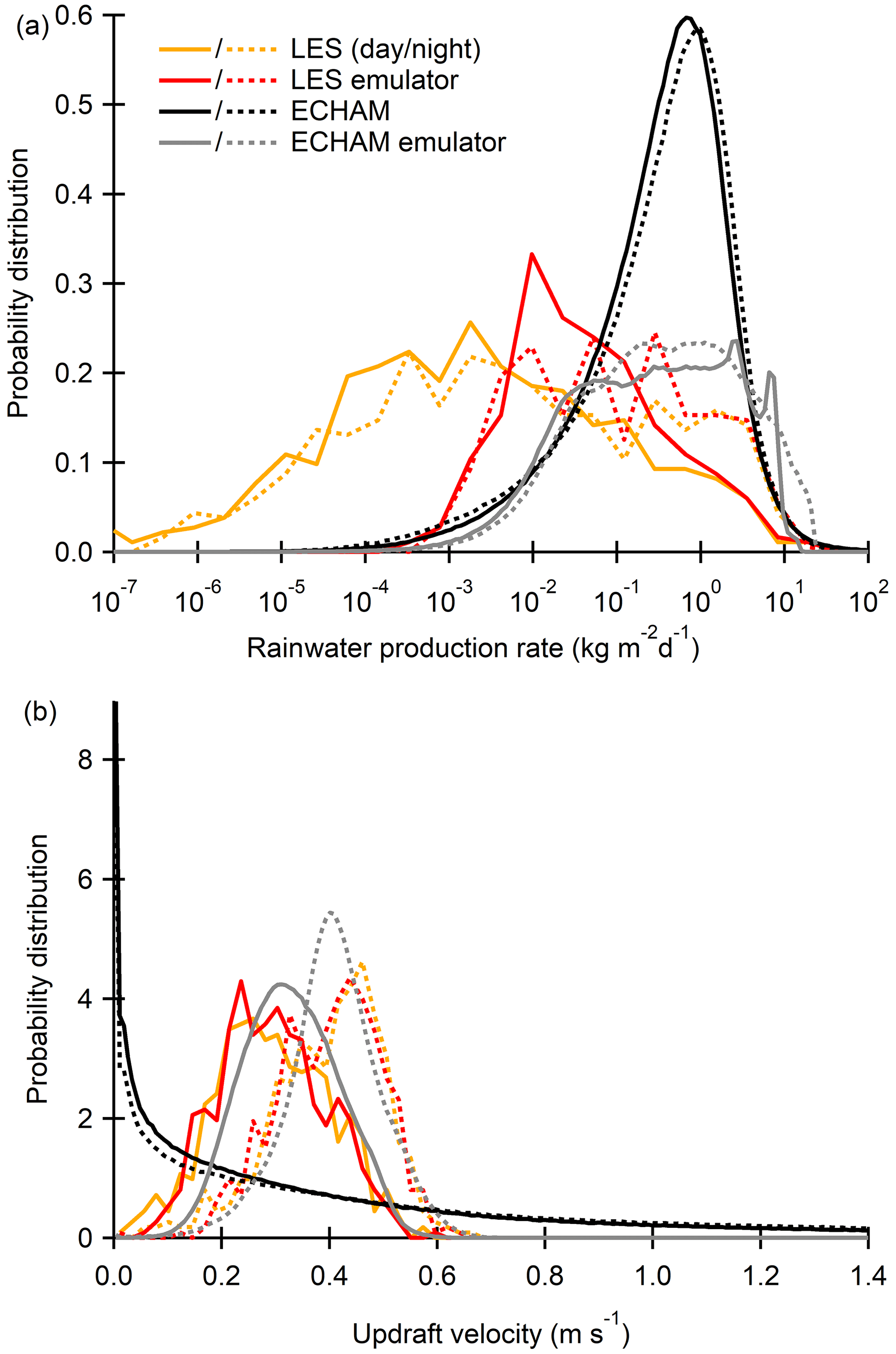
Figure 3Distributions of rainwater production rates (a) and updraft velocities (b) from the LES (orange), the LES emulator (red), ECHAM (black), and the emulators implemented in ECHAM (gray). Solid and dashed lines are for daytime and nighttime distributions, respectively.
Comparison between LES and ECHAM shows that the rainwater production rates from ECHAM are generally higher than those from the LES (Fig. 3a). On the other hand, the default ECHAM values and the ECHAM emulator-based rates have similar magnitudes, but the emulator-based rates have lower frequencies due to the missing values smaller than 10−3 . Overall, the lower likelihood means that the rainwater production emulator reduces precipitation. This is most likely due to the fact that the idealized cloud-topped marine boundary layer initial setting for the LES simulations favors drizzle if any precipitation at all. In contrast, the ECHAM data can include some less-ideal and more heavily precipitating cases (e.g., cases influenced by synoptic-scale weather systems).
The distributions of updraft velocities from the LES (and the emulators) differ from those from ECHAM, which are dominated by small values but have occasionally extremely high values exceeding 10 m s−1 (Fig. 3b). Due to these high values the average vertical velocity is 0.6 m s−1. Both the high and low values are missing from the LES distributions. The LES and the emulators show that daytime and nighttime updraft distributions differ, which is not seen in ECHAM. Lower daytime updrafts can be expected, because solar radiation reduces cloud-top radiative cooling, which is one of the main mechanism generating turbulence in marine environments (e.g., Lilly, 1968). Overall, the updraft velocity emulators are able to produce reasonable updraft velocity distributions and also account for the differences between day and night (Zheng et al., 2016), thus improving the realism of the ECHAM simulation in this respect.
3.2 Cloud regions for the emulators
Figure 4 depicts how often the emulators were applied or could have been applied in the different simulations, i.e., how often the criteria outlined in Sect. 2.2 are met in each model run. Although the emulation criteria are not the same as those used to identify stratocumulus clouds, the frequency of emulator calls (18.8 %–21.2 %) corresponds well with the estimated stratocumulus coverage of 23 % over oceans (Wood, 2012). The emulation criteria are met most frequently at midlatitudes and in the marine regions west from North and South America and Africa, which are known for persistent stratocumulus cloud decks (Struthers et al., 2013; Neubauer et al., 2014). We will be referring to these three specific regions as Californian, Peruvian, and Namibian stratocumulus regions. The geographical extent of these areas is depicted in Fig. 4 based on the boundaries defined by Partanen et al. (2012). Over these three regions the emulators were applied more than 40 % of the time.
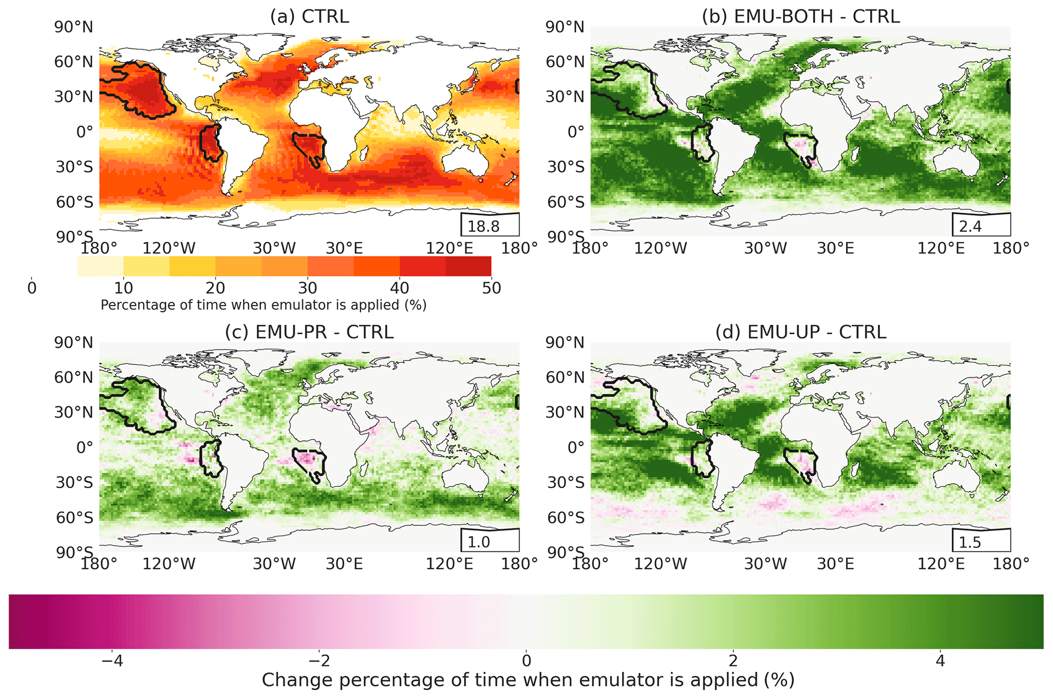
Figure 4Percentage of model time steps when the emulator could have been or has been called in each marine column in simulation (a) CTRL, (b) EMU-BOTH, (c) EMU-PR, and (d) EMU-UP. Panel (a) shows the absolute values for CTRL, while panels (b)–(d) show the difference from the CTRL (note the different color scales). The insets show the mean percentages over the marine columns. The boundaries of the Californian, Peruvian, and Namibian stratocumulus regions as defined by Partanen et al. (2012) are shown with thick lines.
The frequency at which the emulators are used (or could be used, for CTRL) differs between the four simulations. This means that the use of the emulators impacts atmospheric conditions and cloud properties and hence affects when the criteria for calling the emulators are met in the subsequent time steps. Overall, using any emulator increases the frequency from 18.8 % of the CTRL simulation. In the simulation EMU-PR (Fig. 4c), the emulation criteria are met on average 19.8 % of the time in marine columns, and the number increases to 20.3 % in EMU-UP (Fig. 4d). It is also consistent that applying both emulators simultaneously (simulation EMU-BOTH, Fig. 4b) leads to a value of 21.2 %, which is higher than those from the separate emulators.
3.3 The impact of the emulators on climate simulations
In this section, the impacts of the emulators on the climate simulated by ECHAM are reported. Specifically, we examine how the different emulator combinations affect clouds, surface precipitation, cloud shortwave radiative effects, and aerosol effective radiative forcing estimates. Section 3.3.5 shows how the emulators affect the climate sensitivity of ECHAM.
3.3.1 Clouds
The emulators have direct and indirect impacts on various cloud variables, and here we show their impacts on mean cloud cover (Fig. 5 and Table 2) and LWP (Table 3). The tables show area-weighted mean values from simulations and observations for the three stratocumulus regions shown in Fig. 4 and the global mean. ECHAM cloud cover is evaluated using the maximum–random overlap assumption, without applying a satellite simulator. It is acknowledged that this brings some uncertainty to the comparison with satellite data.
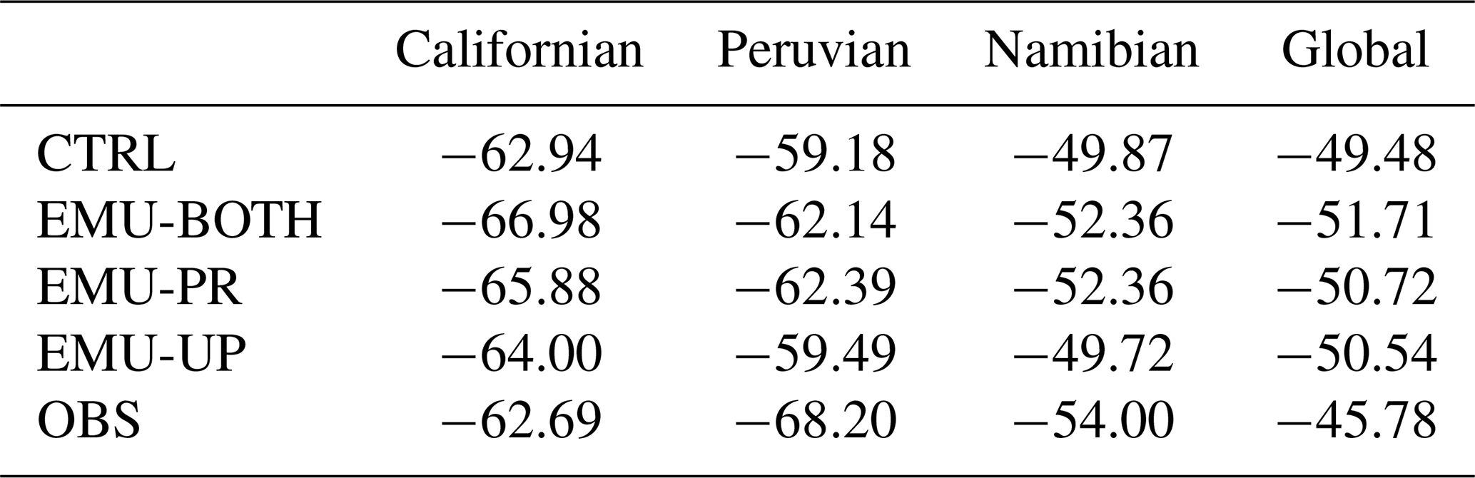
Table 2Mean cloud cover for the three stratocumulus regions and globally from the three different emulator configurations, control run, and from observations.
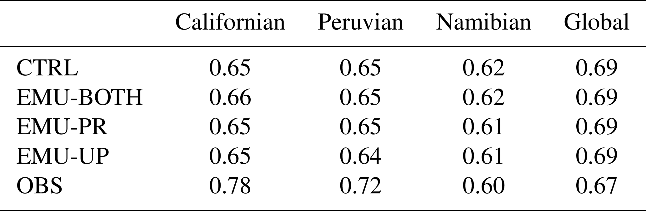
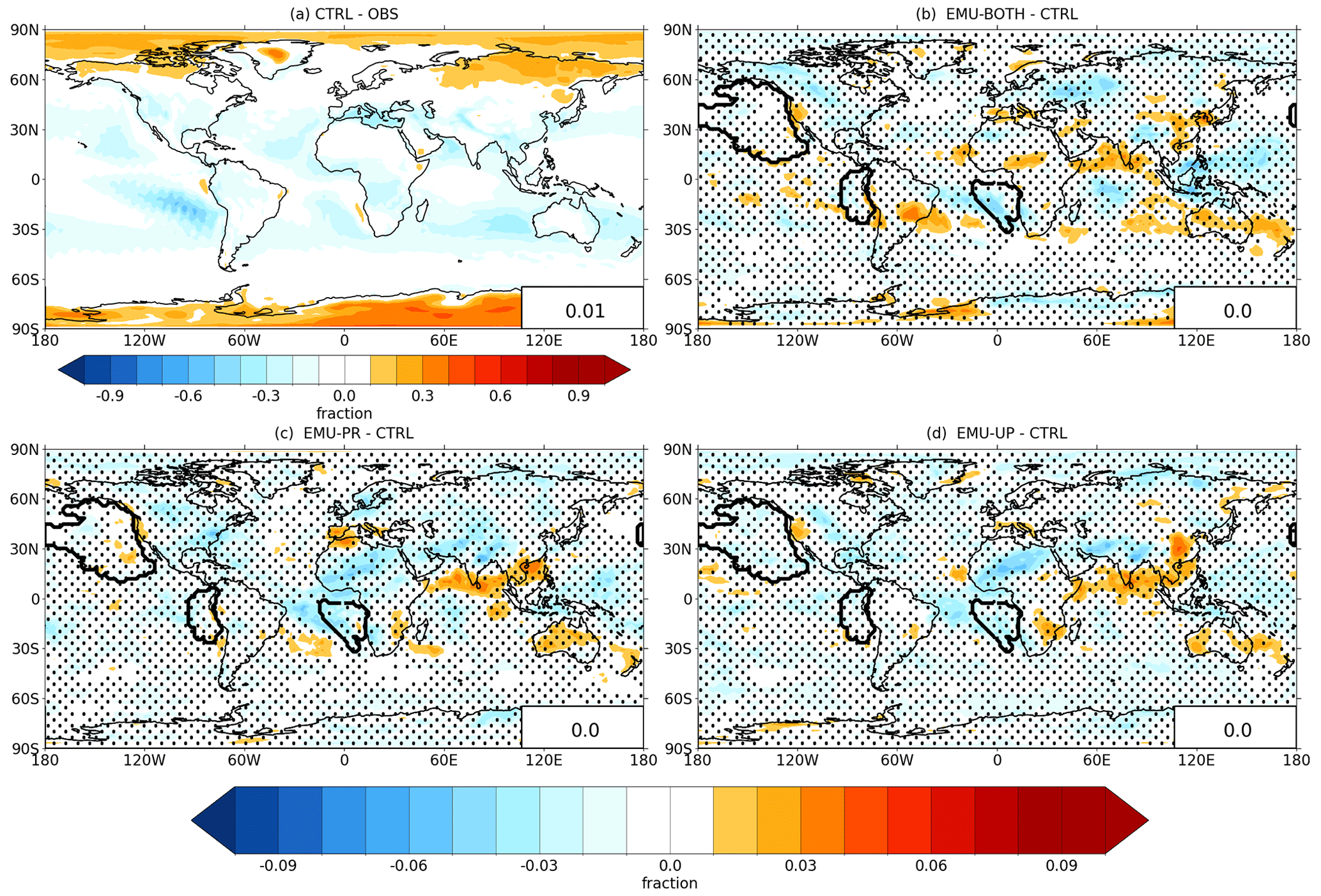
Figure 5Comparison of annual mean cloud fraction between (a) the CTRL simulation and observations, (b) CTRL and EMU-BOTH, (c) CTRL and EMU-PR, and (d) CTRL and EMU-UP. Dots indicate areas where the difference is not statistically significant at p > 0.05. Identified marine stratocumulus regions are shown in each panel with thick black lines. Global-mean values are shown in the lower-right corners.
Figure 5 and Table 2 show that while the control simulation captures the observed global annual mean cloud cover well (with a bias of 0.01), the regional biases can be larger. It is evident that the emulators have only a small impact on cloud cover and that they do not consistently improve or worsen the agreement with observations. This is also seen in Table 4, where correlation coefficients and root mean square errors between observations and different simulations are almost the same.
Table 3Mean LWP (g m−2) for the three stratocumulus regions and globally from the three different emulator configurations, control run, and from observations.
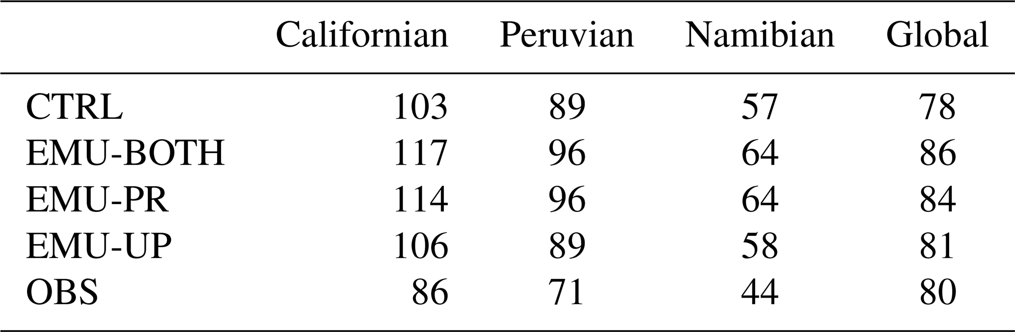
Table 4Correlation coefficient (r) and root mean square error (RMSE) between observations and the control run and the three different emulator configurations.
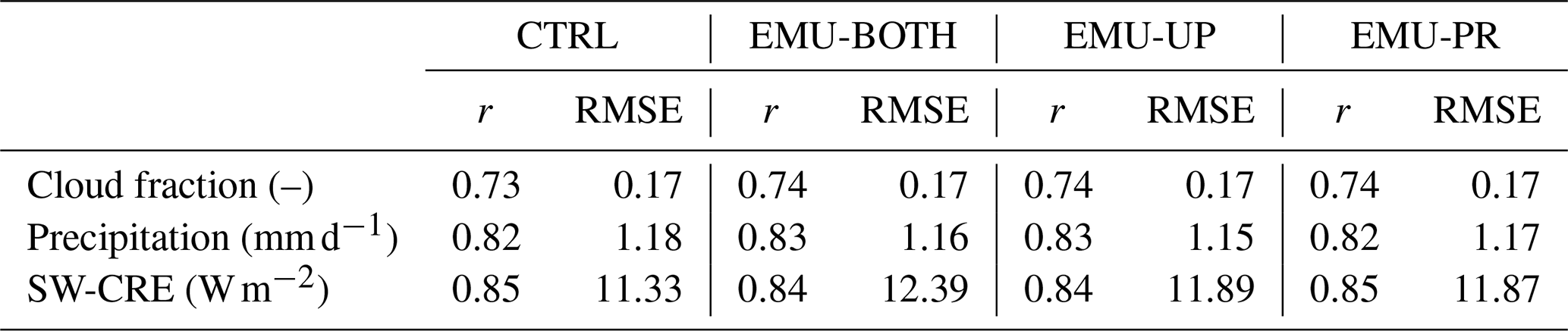
Table 3 shows that in the EMU-BOTH and EMU-PR experiments, cloud LWP is significantly larger than in the CTRL experiment, while EMU-UP is close to CTRL. This can be explained based on Fig. 3, which shows that the precipitation emulator produces less rainwater than the original ECHAM parameterization. Since the long-term and large-scale averages of precipitation are largely controlled by surface evaporation, which changes only slightly between the different ECHAM experiments, it follows that also precipitation can only change slightly. Therefore, when using the precipitation emulator, a larger cloud liquid water amount is maintained, and it generates a precipitation amount close to that in CTRL. It is also seen from Table 3 that the LWP values for EMU-BOTH and EMU-PR clearly exceed the observational estimate for the three stratocumulus regions.
Some further insight on the impact of the emulator on cloud-related quantities is obtained by considering their vertical profiles. Fig. 6 shows the profiles of cloud water mixing ratio, CDNC, updraft velocity, and cloud fraction for the three stratocumulus regions from the four ECHAM simulations. Compared to CTRL, lower maximum updraft peaks can be seen for EMU-UP and EMU-BOTH for the clouds below 850 hPa in column 3. This is related to the distribution of the emulator-based updraft velocities, which have lower mean values than those from ECHAM (Fig. 3). The highest updraft velocities below 850 hPa thus decrease when using the updraft emulator, and this leads to decreased CDNC in these model layers. The updraft emulator has an opposite effect at altitudes above 850 hPa. However, for clouds at these altitudes, the emulator is used less frequently than for clouds at lower levels, and, therefore, emulator impacts on the average updraft velocity become less clear. For this reason all ECHAM experiments have similar rather small updraft velocities above 850 hPa and also the CDNC values become more similar. Consistent with the LWP values discussed above, the use of the precipitation emulator results in clearly higher cloud water content, especially below 850 hPa. While the clouds in the Peruvian and Namibian stratocumulus regions occur mostly below 850 hPa, clouds in the Californian stratocumulus region reach altitudes above 850 hPa, which explains the relatively high precipitation rates examined in the next section. Overall, the emulators have a negligible effect on cloud cover as seen in panels d, h, and l.
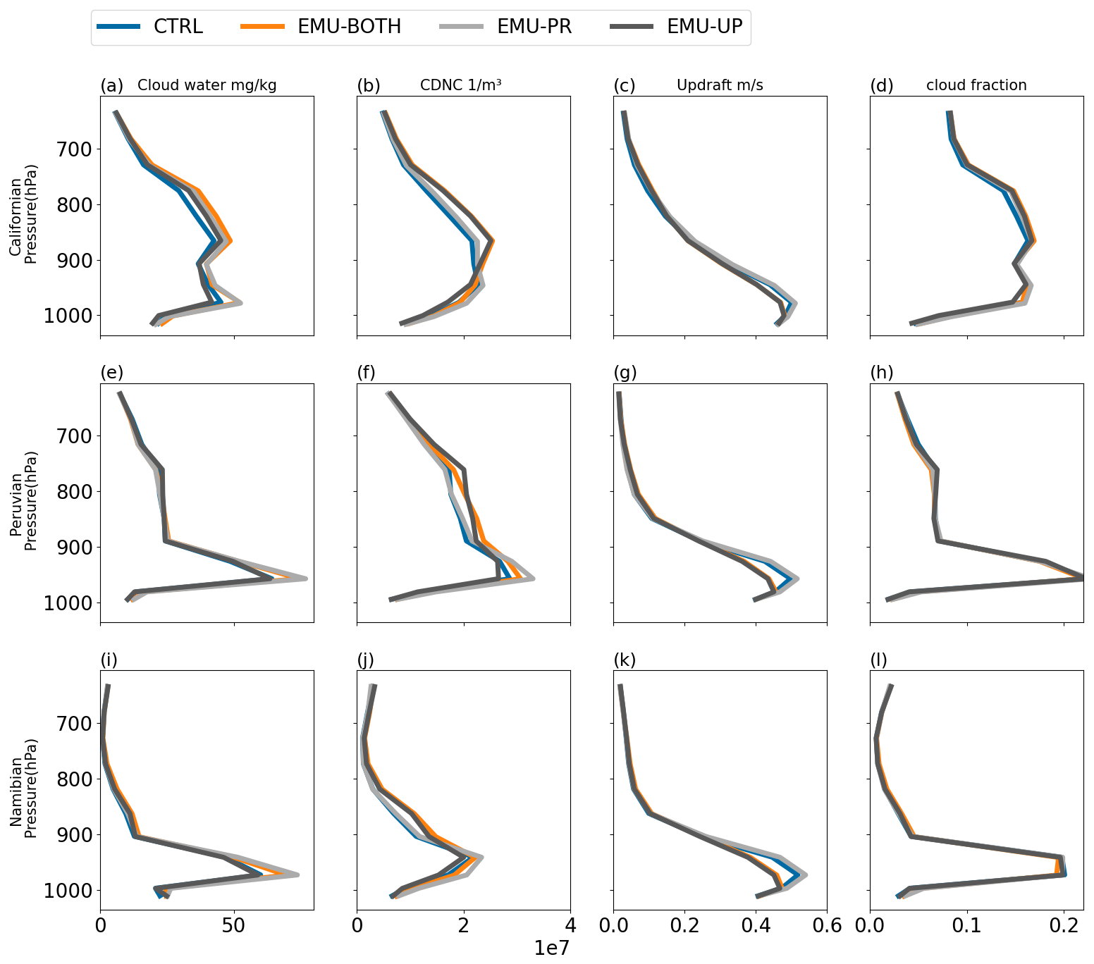
Figure 6Vertical profiles of cloud water (column 1), cloud droplet number concentration (CDNC; column 2), updraft velocity (column 3), and cloud fraction (column 4) for the three stratocumulus regions (rows 1–3). Each line represents a different emulator configuration: CTRL (blue), EMU-BOTH (orange), EMU-PR (gray), and EMU-UP (black).
3.3.2 Precipitation
Figure 7a illustrates the bias in the CTRL simulation compared to the observed surface precipitation. The CTRL experiment overestimates precipitation over large areas of the tropical oceans, especially in the Indian and Pacific oceans. The global average bias is 0.29 mm d−1. Panels b–d show the impacts of the emulators on precipitation simulated by ECHAM (note the different color scale). Globally, the impact of the emulators is small as most of the time the emulator is not applied. The local precipitation biases are reduced slightly in some regions but increased in others. Table 4 shows correlation coefficients between observations and simulated precipitation for all four experiments. Here, the emulators tend to slightly increase the correlation coefficients and decrease RMSE.
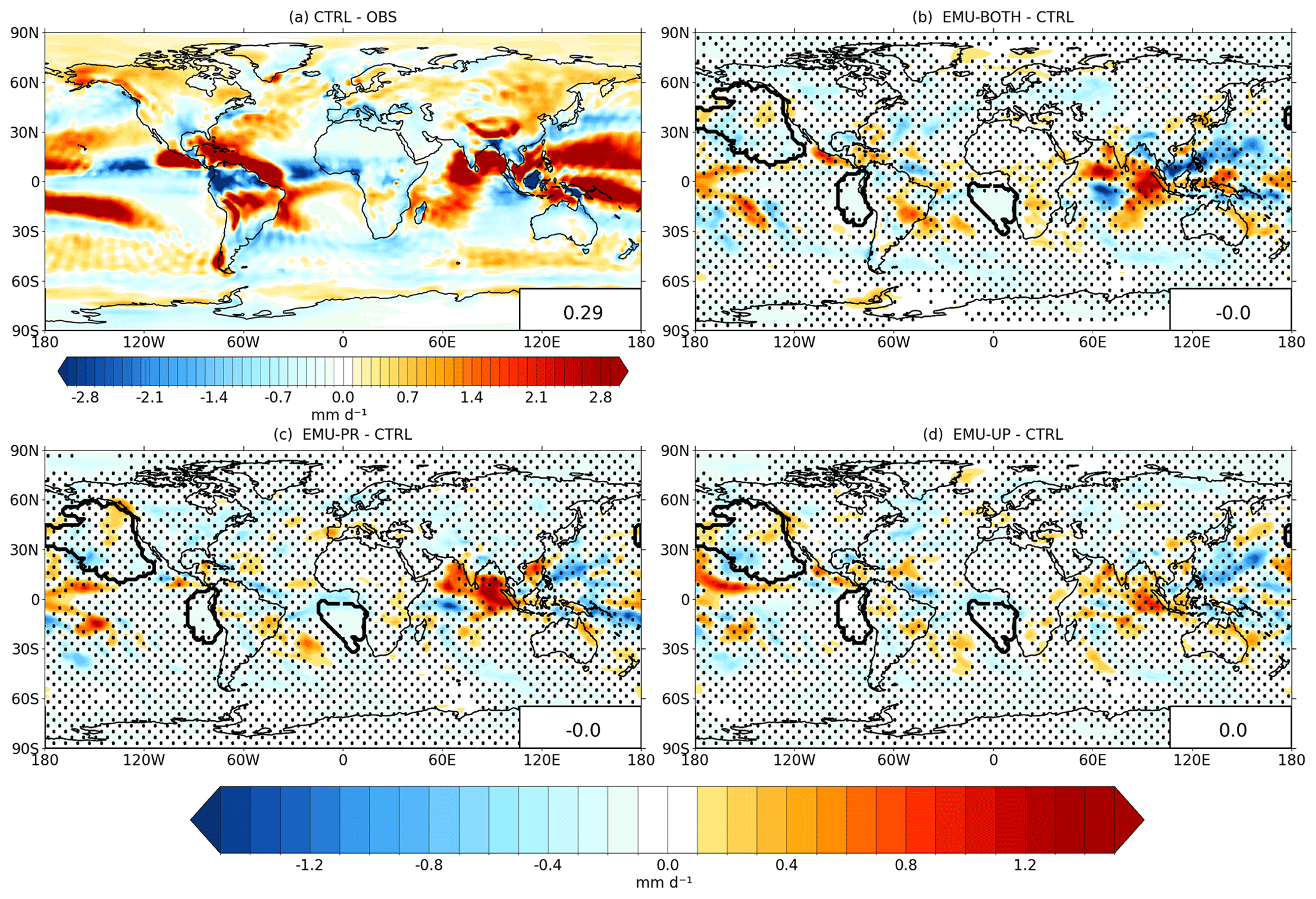
Figure 7Comparison of annual mean surface precipitation (mm d−1) between (a) the CTRL simulation and observations, (b) CTRL and EMU-BOTH, (c) CTRL and EMU-PR, and (d) CTRL and EMU-UP. Dots indicate areas where the difference is not statistically significant at p > 0.05. Identified marine stratocumulus regions are shown in each panel with thick black lines. Global-mean values are shown in the lower-right corners.
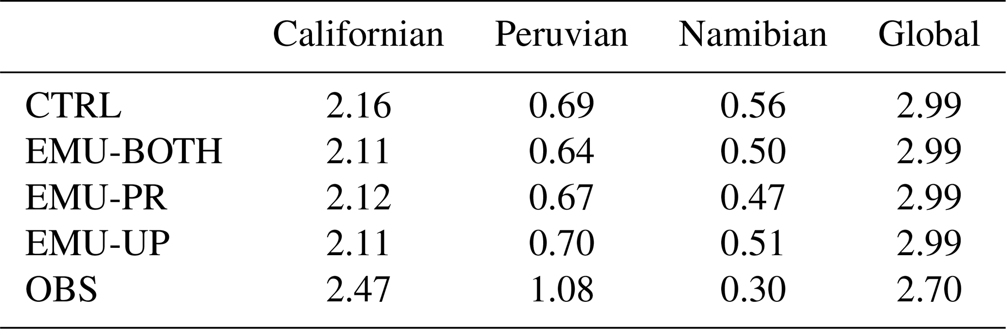
In the three persistent stratocumulus regions (Californian, Peruvian, and Namibian), shown in Figs. 7b–c and in Table 5, the emulators impact the simulated precipitation quite little in absolute terms. This is expected as precipitation rates from the shallow stratocumulus clouds are typically low as shown in Table 5. The Californian stratocumulus region is an exception because the selected region extends from the dry Californian coast up to the South coast of Alaska where precipitation rates are significantly higher due to the frequent occurrence of mid-latitude low-pressure systems (see Fig. 6a). All emulators reduce the clear positive bias in the Namibian stratocumulus region, where the mean surface precipitation rates are the lowest. On the other hand, all emulators increase the negative bias in the Californian stratocumulus region, where the mean surface precipitation rates are the highest. For the Peruvian stratocumulus region, the emulators have both negative and positive impacts on the precipitation bias.
Table 5Mean surface precipitation (mm d−1) for the three stratocumulus regions and globally from the three different emulator configurations, control run, and from observations.
3.3.3 Shortwave cloud radiative effects
Figure 8 shows how well the standard ECHAM produces the observed shortwave cloud radiative effect (SW-CRE) and how each applied emulator (EMU-ALL, EMU-PR, and EMU-UP) affects the SW-CRE prediction (note the different color scales). The ECHAM CTRL run captures the observed SW-CRE quite well, although with a slight negative bias in most regions, which results in a global-mean bias of −3.71 Wm−2.
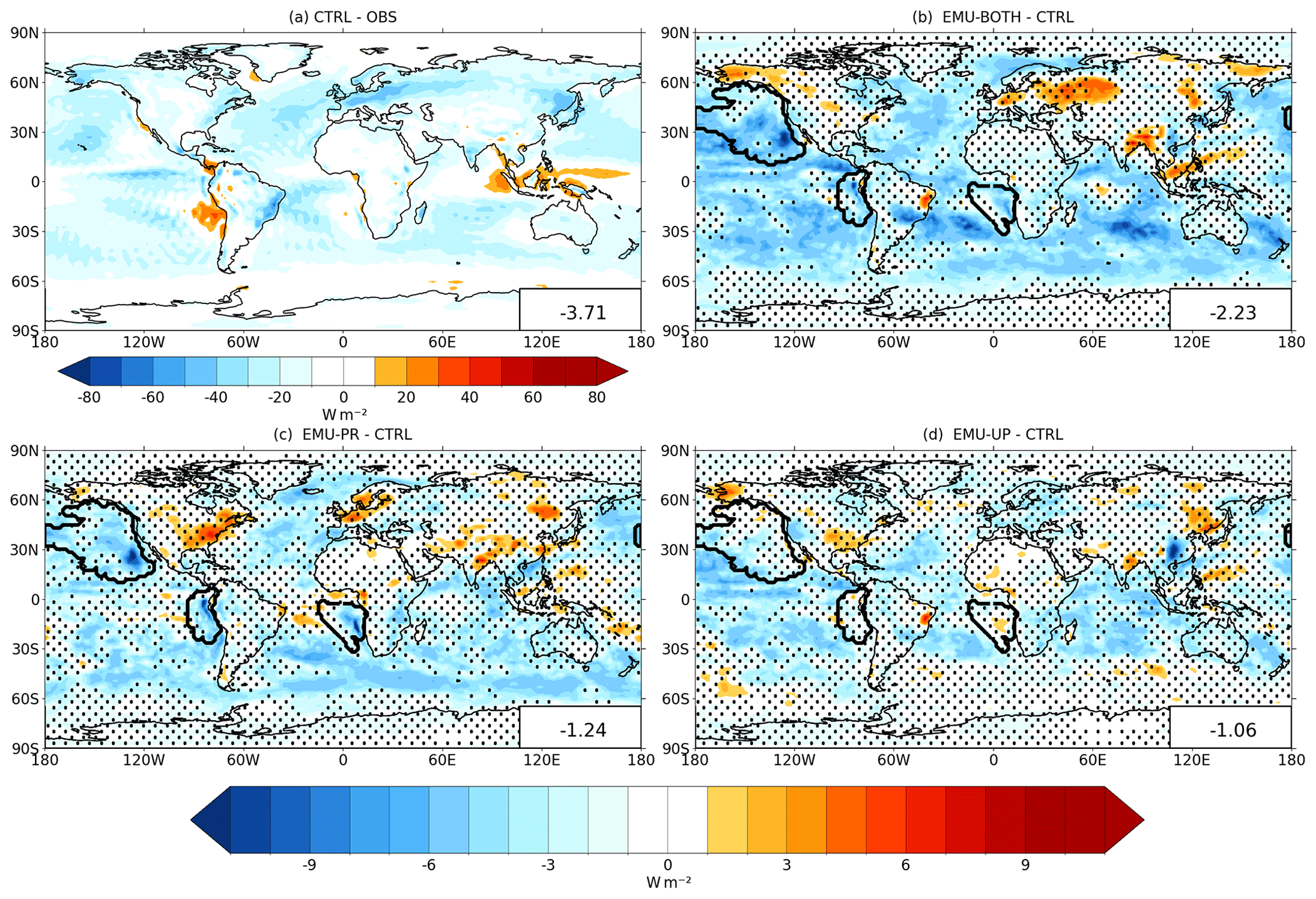
Figure 8Comparison of annual mean SW-CRE between (a) CTRL simulation and observations, (b) CTRL and EMU-BOTH, (c) CTRL and EMU-PR, and (d) CTRL and EMU-UP. Dots indicate areas where the difference is not statistically significant at p > 0.05. Identified marine stratocumulus regions are shown in panels (b)–(d). Global-mean values are shown in the lower-right corners.
All emulators increase the negative global-mean bias by 1.06–2.23 W m−2, with the largest impacts from EMU-BOTH and EMU-PR. The stronger negative SW-CRE in these experiments is primarily caused by the increased LWP (see Table 3). The stronger SW-CRE is mostly seen over mid- and high-latitude marine regions. For example,the Southern Ocean is heavily affected by the precipitation emulator producing a more negative SW-CRE. Table 4 shows correlation coefficients and RMSE between observations and different simulations. The emulators have little effect on the correlations; however, using the emulators increases the RMSE compared to the CTRL simulation.
Although the emulators increase the global-mean bias, each emulator has a distinct effect on the three stratocumulus regions as shown in Figs. 8b–d. To clarify the differences between the simulations, mean SW-CRE values were calculated for each region, and these are shown in Table 6. Although the global-mean bias is negative in CTRL, the bias is positive in the Peruvian and Namibian stratocumulus regions and negative only in the Californian stratocumulus region. Therefore, the increased negative SW-CRE in EMU-PR and EMU-BOTH acts to reduce the bias for the Peruvian and Namibian stratocumulus regions but increases it in the Californian stratocumulus region.
Table 6Mean SW-CRE values (W m−2) for the three stratocumulus regions and globally from the three different emulator configurations, control run, and from observations.
3.3.4 Aerosol effective radiative forcing
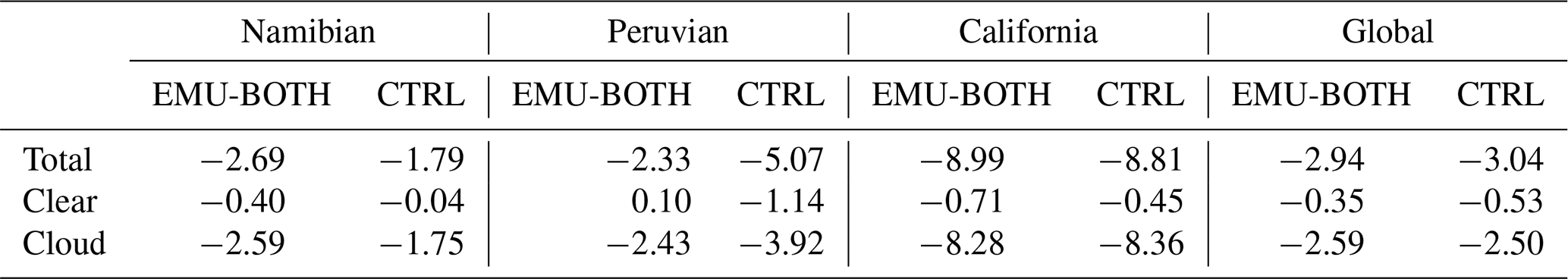
Figure 9 shows the calculated aerosol effective radiative forcing (ERF) based on the present-day and pre-industrial EMU-BOTH and CTRL simulations. The global-mean values (−3.04 W m−2 for CTRL and −2.94 W m−2 for EMU-BOTH) are strongly negative, and their magnitude clearly exceeds the state-of-the-art estimates of ERF (e.g., IPCC AR6 WG1 gives a best estimate of −1.3 W m−2 with a 90 % confidence interval of −2.0 to −0.6 W m−2 over 1750–2014 Masson-Delmotte et al., 2021). The very high negative ERF is due to limiting the minimum value of CDNC to 10 cm−3 instead of 40 cm−3 which is typically used as the lower limit of CDNC in ECHAM. Another factor affecting ERF is the different dependency of autoconversion parameterization on droplet number concentration employed in ECHAM and emulator training.
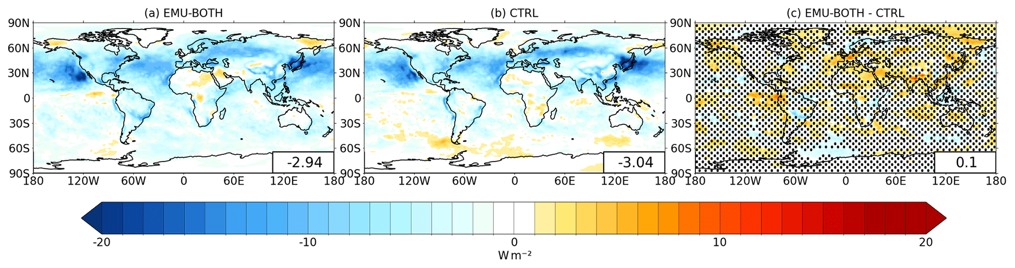
Figure 9Aerosol effective radiative forcing (a) when both precipitation and updraft emulators are applied and (b) based on the control simulation with the standard ECHAM, and (c) the difference between the emulator and control simulations. Global-mean values are shown in the lower-right corners. Dots in panel (c) indicate regions where the difference is not statistically significant at p > 0.05.
Additional details about the aerosol ERF are shown in Table 7, where different components of the ERF are calculated for the three stratocumulus regions and for the whole globe. The impact of the emulators on the aerosol ERF in the stratocumulus regions is non-systematic: the ERF becomes more negative for the Namibian and Californian regions but less negative for the Peruvian region.
Table 7Mean aerosol effective radiative forcing components (W m−2) for the three stratocumulus regions and globally from the emulator and control runs.
3.3.5 Climate sensitivity
The current emulators were trained for the present-day climate, which raises a question about their performance for warmer climates. To test this, we calculated the impact of the emulators on the climate sensitivity of the ECHAM model. Here, climate sensitivity is estimated using inverse climate change experiments (e.g., Cess et al., 1990), in which a climate change is prescribed by increasing the SST by +4 K and the response in TOA net radiation and near-surface air temperature are evaluated. The climate sensitivity parameter λ is then calculated as
where ΔT and ΔFnet are global-mean changes in the near-surface air temperature and TOA net radiation. Here, ΔT and ΔFnet are evaluated based on the difference between WARM and present-day simulations, separately for the control version of ECHAM (WARM-CTRL vs. CTRL) and for the version that uses both the precipitation and updraft emulators (WARM-EMU-BOTH vs. EMU-BOTH).
Figure 10 shows the change in the TOA net radiation (ΔFnet) when emulators are used (panel a) and without emulators (panel b). Although the regional differences (panel c) are not statistically significant, the simulation with emulators tends to produce less negative forcing over the Southern Hemisphere. The global-mean ΔT values for WARM-EMU-BOTH and WARM-CTRL are 4.47 and 4.46 K, which results in climate sensitivity parameters of λ=0.62 and λ=0.57 , respectively. Thus, because of the smaller TOA net flux response, the climate sensitivity is somewhat higher when the emulators are applied.
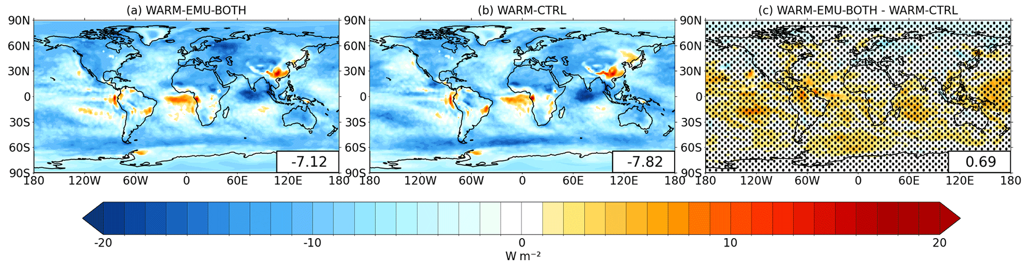
Figure 10The change in TOA net radiation resulting from a +4 K SST change: (a) when both updraft and precipitation emulators are used, (b) based on the control simulation, and (c) the difference between these two. Dots in panel (c) indicate regions where the difference is not statistically significant at p > 0.05.
Figure 11 displays the changes in precipitation and shortwave cloud radiative effect (SW-CRE) in the warm climate simulations. In these simulations, when the climate becomes warmer, changes in precipitation are not significantly influenced by the use of the emulators. The patterns of change in SW-CRE from the control climate to the warmer climate state are also very similar irrespective of whether the emulators are employed or not, but the global-mean change in SW-CRE is more positive when the emulators are used (+2.1 W m−2) than for the default model version (+1.4 W m−2).
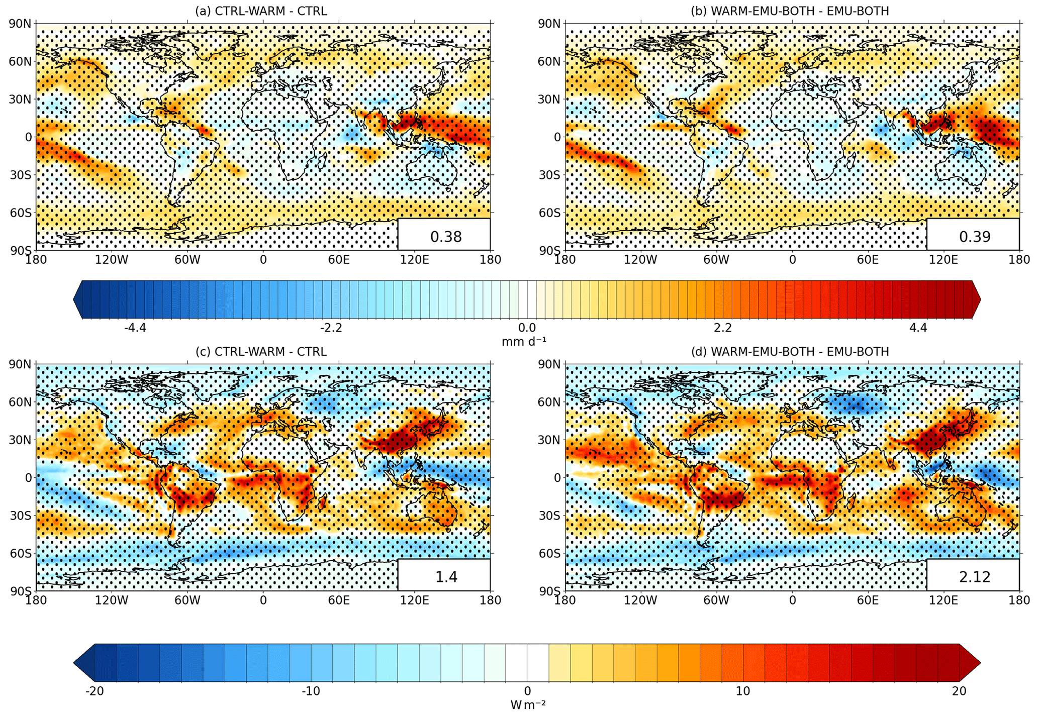
Figure 11Panels (a) and (b) show the change in annual mean precipitation for +4 K SST change without the emulator (a) and with both the updraft and precipitation emulator (b). Panels (c) and (d) show the same as above but for SW-CRE. Dots indicate regions where the difference is not statistically significant at p > 0.05.
Overall, while internal variability makes it challenging to robustly identify small changes in model behavior in 10-year experiments, it can be stated that the emulators have only a modest impact on the modeled climate response. This suggests that these emulators can be used safely for climate states that are, at least, 4 K warmer than the baseline climate from which the training data for the emulators were sampled.
In this proof-of-concept study we have shown the applicability of LES-based emulators for precipitation and cloud base updraft velocity predictions in the general circulation model ECHAM. Our simulations are stable and the emulators have a negligible impact on the simulation time. In fact, most of the computational time was spent in developing the emulator, which essentially means generating the training data. Applying the emulator to stratocumulus clouds has a relatively small impact on ECHAM simulations, and it is hard to say whether the results are improved or not. The standard ECHAM is tuned so that it matches with observations as well as possible, so even an improved description of processes like precipitation and updraft velocity can reduce the agreement with observations. More quantitative assessment of the potential improvements would have required model re-tuning which is beyond the scope and technical resources of this proof-of-concept study. This would impact results as the stratiform rain formation rate by autoconversion, entrainment rate for shallow convection, entrainment rate for deep convection, and convective conversion rate from cloud water to rain are part of the ECHAM6 tuning strategy (Neubauer et al., 2019).
One limitation in developing LES-based emulators for a GCM is that there is a gap in the modeled scales. When a large ensemble of training simulations is needed, the LES especially with detailed microphysics is limited to about a 10 km × 10 km domain, while most GCMs (including ECHAM) have a grid size in the order of 100 km × 100 km. Most previous studies have used cloud-resolving models (CRMs), which can easily represent a column of a global model. However, CRMs often use similar parameterizations as GCMs, so a LES is needed for real improvements in accounting for turbulence and the details of the aerosol–cloud–precipitation interactions. The high computational cost of using LES with detailed aerosol microphysics limits its use in the emulator development (Ahola et al., 2022), so in this study we did not account for the aerosol effects. Nevertheless, the approach used here is a promising candidate for the detailed representation of aerosol- and cloud-related sub-grid processes.
Just like in many other GCMs with computationally expensive aerosol microphysics enabled, coarse vertical resolution is used in the current ECHAM setup. This limits the model's capabilities in reproducing realistic stratocumulus cloud decks (Neubauer et al., 2014), which is an issue for generating the LES input profiles. For that we had to assume a well-mixed cloud-topped boundary layer. Sufficiently high GCM grid resolutions are available only for certain high-resolution model configurations without aerosol microphysics (Chang et al., 2020). Thanks to the increasing computing power, future GCMs can have higher resolution even with aerosol microphysics enabled. In summary, developing LES-based emulators for aerosol–cloud interactions should become easier in the future.
Another issue that is related to the different scales of LES and GCM is the definition of the model parameters. For example, there are different definitions for the mean or characteristic cloud base updraft velocity (Romakkaniemi et al., 2009). Precipitation is even more dependent on model scales and definitions, but at the same time there is great potential for improvements. This is because precipitation is diagnostic in ECHAM, but the LES can include the impacts of sub-grid variability as well as time and aerosol dependency of rain drop size development as an example. Employing such simulations to train the emulator would add physical realism into large-scale models and reduce the number of commonly employed model tuning parameters needed to reproduce observed cloud cover and properties.
Current emulators produce scalar outputs, such as characteristic updraft velocity, but it would be possible to train additional emulators for distribution parameters like standard deviation or skewness. Indeed, some models (e.g., Golaz et al., 2011) utilize sub-grid-scale updraft velocity distributions in calculating CDNC. Due to the nonlinear dependency of activation on vertical velocity, calculations based on a characteristic value and a distribution produce different CDNC.
In broader terms, the main issue in developing a LES-based emulator for a GCM is in finding suitable GCM variables and translating LES outputs into consistent emulator outputs. Surely, not all GCM variables are suitable for emulation, or at least require specific LES setup, and likewise the LES is not the best tool to generate training data for some variables. Even when variables seem consistent, this has to be carefully checked. For example, we had to choose from different updraft velocity definitions the one that matches with the one used in the ECHAM cloud scheme. The LES setup in this case mimics steady-state cloud, where updrafts and rain rate formation rates are fairly constant. Obviously this setup is not valid for parameters like cloud cover, which requires transient simulations. Overall, there are many things that have to be considered case by case, but the LES-emulation approach should be a good starting point for most cases.
Finally, there are different machine learning methods that can be used for representing LES simulations. For example, we used random forest successfully in our previous study (Ahola et al., 2022). Nevertheless, the binary space partitioning (BSP) sampling combined with the Gaussian process emulation (GPE) technique seems an advantageous combination for our purpose. The BSP method can be used to sample a representative set of the GCM columns based on their likelihood. This means that the emulator is more accurate for those points where the emulator is called most frequently while larger uncertainty is tolerated for outliers. The GPE technique is suitable for the computationally expensive LES runs requiring, at minimum, only 10 simulations per variable.
Here in this proof-of-concept study we presented the first results of using LES-based precipitation and cloud base updraft velocity emulators in the ECHAM general circulation model simulations. We showed that the emulators, which were applied only to marine stratocumulus clouds, have a small but statistically significant influence on ECHAM simulations. Although the emulation approach has some practical difficulties and limitations, the traditional parameterizations based on simple mathematical functions are not suitable for representing complex dependencies like the output of a LES run. The main advantage of the method is that the LES can account for turbulence and cloud interactions, which are highly parameterized sub-grid-scale processes in any large-scale model. The level of details that can be accounted for is largely limited by the LES simulations and their computational costs. In this case, the high computational costs forced us to ignore aerosol–cloud interactions, but the approach is applicable to them as well. In addition, emulators can be trained for presenting other processes than precipitation or cloud-scale updrafts depending on current aims and on the global model. For example, improving mixed-phase cloud physics using LES-based emulators could be the next step ahead.
The LES outputs and ECHAM simulations used in generating the emulator training data can be found in Ahola et al. (2022) and references therein. The codes and the data used in emulator development and validation as well as the ECHAM implementation are available from https://github.com/kallenordling/eclair_emulator (last access: 4 April 2023; https://doi.org/10.5281/zenodo.10208603, Nordling, 2023). ECHAM simulation results are available from http://urn.fi/urn:nbn:fi:att:c6c6c7b3-38d1-47f8-9c46-fe5761554bea (Nordling, 2023). The ECHAM6-HAMMOZ code is maintained and made available to the scientific community under https://redmine.hammoz.ethz.ch/projects/hammoz/ (HAMMOZ consortium, 2023a). The availability is regulated under the HAMMOZ Software Licence Agreement that can be downloaded from https://redmine.hammoz.ethz.ch/attachments/download/291/License_ECHAM-HAMMOZ_June2012.pdf (HAMMOZ consortium, 2023b). The UCLALES-SALSA source code is available from https://doi.org/10.5281/zenodo.5289397 (Tonttila et al., 2021).
KN developed the emulators with help from TR, JPK, MEA, and JA. KN made the ECHAM simulations with help from JPK, HarK, and PR. KN and TR wrote the paper with help from HarK, SR, TR, PR, AL, and HanK. All authors commented on the manuscript. HanK came up with the original concept.
The contact author has declared that none of the authors has any competing interests.
Publisher’s note: Copernicus Publications remains neutral with regard to jurisdictional claims made in the text, published maps, institutional affiliations, or any other geographical representation in this paper. While Copernicus Publications makes every effort to include appropriate place names, the final responsibility lies with the authors.
The authors wish to acknowledge CSC – IT Center for Science, Finland, for computational resources.
This research has been supported by the European Research Council, H2020 (grant nos. 646857 and 821205), and the Academy of Finland (grant nos. 322532, 309127, and 337552).
This paper was edited by Paulo Ceppi and reviewed by three anonymous referees.
Abdul‐Razzak, H. and Ghan, S. J.: A parameterization of aerosol activation 3. Sectional representation, J. Geophys. Res.-Atmos., 107, 4026, https://doi.org/10.1029/2001JD000483, 2002. a, b
Abdul-Razzak, H., Ghan, S. J., and Rivera-carpio, C.: A parameterization of aerosol activation: 1. Single aerosol type, J. Geophys. Res., 103, 6123–6131, https://doi.org/10.1029/97JD03735, 1998. a
Adler, R. F., Gu, G., and Huffman, G. J.: Estimating climatological bias errors for the Global Precipitation Climatology Project (GPCP), J. Appl. Meteorol. Clim., 51, 84–99, https://doi.org/10.1175/JAMC-D-11-052.1, 2012. a
Ahola, J., Raatikainen, T., Alper, M. E., Keskinen, J.-P., Kokkola, H., Kukkurainen, A., Lipponen, A., Liu, J., Nordling, K., Partanen, A.-I., Romakkaniemi, S., Räisänen, P., Tonttila, J., and Korhonen, H.: Technical note: Parameterising cloud base updraft velocity of marine stratocumuli, Atmos. Chem. Phys., 22, 4523–4537, https://doi.org/10.5194/acp-22-4523-2022, 2022. a, b, c, d, e, f, g, h, i, j, k, l, m
Besombes, C., Pannekoucke, O., Lapeyre, C., Sanderson, B., and Thual, O.: Producing realistic climate data with generative adversarial networks, Nonlin. Processes Geophys., 28, 347–370, https://doi.org/10.5194/npg-28-347-2021, 2021. a
Bogenschutz, P. A., Gettelman, A., Morrison, H., Larson, V. E., Craig, C., and Schanen, D. P.: Higher-order turbulence closure and its impact on climate simulations in the Community Atmosphere Model, J. Climate, 26, 9655–9676, https://doi.org/10.1175/JCLI-D-13-00075.1, 2013. a
Boucher, O., Randall, D., Artaxo, P., Bretherton, C., Feingold, G., Forster, P., Kerminen, V.-M., Kondo, Y., Liao, H., Lohmann, U., Rasch, P., K. Satheesh, S., Sherwood, S., Stevens, B., and Zhang, X.: Clouds and Aerosols, Climate Change 2013: The Physical Science Basis. Contribution of Working Group I to the Fifth Assessment Report of the Intergovernmental Panel on Climate Change, http://www.ipcc.ch/pdf/assessment-report/ar5/wg1/WG1AR5_Chapter07_FINAL.pdf (last access: 5 May 2023), 2013. a
Bougiatioti, A., Nenes, A., Lin, J. J., Brock, C. A., de Gouw, J. A., Liao, J., Middlebrook, A. M., and Welti, A.: Drivers of cloud droplet number variability in the summertime in the southeastern United States, Atmos. Chem. Phys., 20, 12163–12176, https://doi.org/10.5194/acp-20-12163-2020, 2020. a
Brenowitz, N. D., Beucler, T., Pritchard, M., and Bretherton, C. S.: Interpreting and Stabilizing Machine-Learning Parametrizations of Convection, J. Atmos. Sci., 77, 4357–4375, https://doi.org/10.1175/JAS-D-20-0082.1, 2020. a
Bretherton, C. S., Henn, B., Kwa, A., Brenowitz, N. D., Watt-Meyer, O., McGibbon, J., Perkins, W. A., Clark, S. K., and Harris, L.: Correcting Coarse-Grid Weather and Climate Models by Machine Learning From Global Storm-Resolving Simulations, J. Adv. Model. Earth Sy., 14, e2021MS002794, https://doi.org/10.1029/2021MS002794, 2022. a
Cesana, G. V. and Del Genio, A. D.: Observational constraint on cloud feedbacks suggests moderate climate sensitivity, Nat. Clim. Change, 11, 213–218, https://doi.org/10.1038/s41558-020-00970-y, 2021. a
Cess, R. D., Potter, G. L., Blanchet, J. P., Boer, G. J., Del Genio, A. D., Déqué, M., Dymnikov, V., Galin, V., Gates, W. L., Ghan, S. J., Kiehl, J. T., Lacis, A. A., Le Treut, H., Li, Z.-X., Liang, X.-Z., McAvaney, B. J., Meleshko, V. P., Mitchell, J. F. B., Morcrette, J.-J., Randall, D. A., Rikus, L., Roeckner, E., Royer, J. F., Schlese, U., Sheinin, D. A., Slingo, A., Sokolov, A. P., Taylor, K. E., Washington, W. M., Wetherald, R. T., Yagai, I., and Zhang, M.-H.: Intercomparison and interpretation of climate feedback processes in 19 atmospheric general circulation models, J. Geophys. Res.-Atmos., 95, 16601–16615, https://doi.org/10.1029/JD095iD10p16601, 1990. a, b
Chang, P., Zhang, S. Q., Danabasoglu, G., Yeager, S. G., Fu, H. H., Wang, H., Castruccio, F. S., Chen, Y. H., Edwards, J., Fu, D., Jia, Y. L., Laurindo, L. C., Liu, X., Rosenbloom, N., Small, R. J., Xu, G. P., Zeng, Y. H., Zhang, Q. Y., Bacmeister, J., Bailey, D. A., Duan, X. H., DuVivier, A. K., Li, D. P., Li, Y. X., Neale, R., Stossel, A., Wang, L., Zhuang, Y., Baker, A., Bates, S., Dennis, J., Diao, X. L., Gan, B. L., Gopal, A., Jia, D. N., Jing, Z., Ma, X. H., Saravanan, R., Strand, W. G., Tao, J., Yang, H. Y., Wang, X. Q., Wei, Z. Q., and Wu, L. X.: An unprecedented set of high-resolution earth system simulations for understanding multiscale interactions in climate variability and change, J. Adv. Model. Earth Sy., 12, e2020MS002298, https://doi.org/10.1029/2020MS002298, 2020. a
Cheng, T., Peng, Y., Feichter, J., and Tegen, I.: An improvement on the dust emission scheme in the global aerosol-climate model ECHAM5-HAM, Atmos. Chem. Phys., 8, 1105–1117, https://doi.org/10.5194/acp-8-1105-2008, 2008. a
Cheruy, F., Chevallier, F., Morcrette, J.-J., Scott, N. A., and Chédin, A.: Une méthode utilisant les techniques neuronales pour le calcul rapide de la distribution verticale du bilan radiatif thermique terrestre, CR. Acad. Sci. II B, 322, 665–672, 1996. a
Chevallier, F., Chéruy, F., Scott, N. A., and Chédin, A.: A Neural Network Approach for a Fast and Accurate Computation of a Longwave Radiative Budget, J. Appl. Meteorol., 37, 1385–1397, https://doi.org/10.1175/1520-0450(1998)037<1385:ANNAFA>2.0.CO;2, 1998. a
Conibear, L., Reddington, C. L., Silver, B. J., Chen, Y., Knote, C., Arnold, S. R., and Spracklen, D. V.: Statistical emulation of winter ambient fine particulate matter concentrations from emission changes in China, GeoHealth, 5, e2021GH000391, https://doi.org/10.1029/2021GH000391, 2021. a
Donner, L. J., O'Brien, T. A., Rieger, D., Vogel, B., and Cooke, W. F.: Are atmospheric updrafts a key to unlocking climate forcing and sensitivity?, Atmos. Chem. Phys., 16, 12983–12992, https://doi.org/10.5194/acp-16-12983-2016, 2016. a
Elsaesser, G., O’Dell, C., Lebsock, M., and Teixeira, J.: Multisensor advanced climatology mean liquid water path L3 monthly 1 degree × 1 degree V1, Greenbelt, MD, USA, Goddard Earth Sciences Data and Information Services Center (GES DISC) [data set], https://doi.org/10.5067/MEASURES/MACLWPM, 2016. a
Fuchs, H., Kedem, Z. M., and Naylor, B. F.: On Visible Surface Generation by a Priori Tree Structures, SIGGRAPH Comput. Graph., 14, 124–133, https://doi.org/10.1145/965105.807481, 1980. a
Gettelman, A., Hannay, C., Bacmeister, J. T. Neale, R. B., Pendergrass, A. G., Danabasoglu, G., Lamarque, J.-F., Fasullo, J. T., Bailey, D. A., Lawrence, D. M., and Mills, M. J.: High climate sensitivity in the Community Earth System Model version 2 (CESM2), Geophys. Res. Lett., 46, 8329–8337, https://doi.org/10.1029/2019GL083978, 2019.
Glassmeier, F., Hoffmann, F., Johnson, J. S., Yamaguchi, T., Carslaw, K. S., and Feingold, G.: An emulator approach to stratocumulus susceptibility, Atmos. Chem. Phys., 19, 10191–10203, https://doi.org/10.5194/acp-19-10191-2019, 2019. a, b
Golaz, J., Larson, V. E., and Cotton, W. R.: A PDF-based model for boundary layer clouds. Part I: method and model description, J. Atmos. Sci., 59, 3540–3551, https://doi.org/10.1175/1520-0469(2002)059<3540:APBMFB>2.0.CO;2, 2002. a
Golaz, J.-C., Salzmann, M., Donner, L. J., Horowitz, L. W., Ming, Y., and Zhao, M.: Sensitivity of the aerosol indirect effect to subgrid variability in the cloud parameterization of the GFDL atmosphere general circulation model AM3, J. Climate, 24, 3145–3160, https://doi.org/10.1175/2010JCLI3945.1, 2011. a, b, c, d
Grabowski, W. W.: Towards Global Large Eddy Simulation: Super-Parameterization Revisited, J. Meteorol. Soc. Jpn Ser. II, 94, 327–344, https://doi.org/10.2151/jmsj.2016-017, 2016. a
Grabowski, W. W. and Smolarkiewicz, P. K.: CRCP: A cloud resolving convection parameterization for modeling the tropical convecting atmosphere, Physica D, 133, 171–178, https://doi.org/10.1016/S0167-2789(99)00104-9, 1999. a
Guelle, W., Schulz, M., Balkanski, Y., and Dentener, F.: Influence of the source formulation on modeling the atmospheric global distribution of sea salt aerosol, J. Geophys. Res., 106, 27509–27524, https://doi.org/10.1029/2001JD900249, 2001. a
Guo, H., Golaz, J., Donner, L. J., Ginoux, P., and Hemler, R. S.: Multivariate Probability Density Functions with Dynamics in the GFDL Atmospheric General Circulation Model: Global Tests, J. Climate, 27, 2087–2108, https://doi.org/10.1175/JCLI-D-13-00347.1, 2014. a
Guo, Z., Wang, M., Larson, V. E., and Zhou, T.: A cloud top radiative cooling model coupled with CLUBB in the Community Atmosphere Model: Description and simulation of low clouds, J. Adv. Model. Earth Sy., 11, 979–997, https://doi.org/10.1029/2018MS001505, 2019. a
HAMMOZ consortium: ECHAM-HAMOZ model data, https://redmine.hammoz.ethz.ch/projects/hammoz/, last access: 4 April 2023a. a
HAMMOZ consortium: https://redmine.hammoz.ethz.ch/attachments/download/291/License_ECHAM-HAMMOZ_June2012.pdf, last access: 4 April 2023b. a
Han, Y., Zhang, G. J., Huang, X., and Wang, Y.: A Moist Physics Parameterization Based on Deep Learning, J. Adv. Model. Earth Sy., 12, e2020MS002076, https://doi.org/10.1029/2020MS002076, 2020. a
Heinold, B., Tegen, I., Schepanski, K., and Banks, J. R.: New developments in the representation of Saharan dust sources in the aerosol–climate model ECHAM6-HAM2, Geosci. Model Dev., 9, 765–777, https://doi.org/10.5194/gmd-9-765-2016, 2016. a
Hoose, C., Kristjánsson, J. E., Iversen, T., Kirkevåg, A., Seland, Ø., and Gettelman, A.: Constraining cloud droplet number concentration in GCMs suppresses the aerosol indirect effect, Geophys. Res. Lett., 36, L12807, https://doi.org/10.1029/2009GL038568, 2009. a
Jansson, F., van den Oord, G., Pelupessy, I., Grönqvist, J. H., Siebesma, A. P., and Crommelin, D.: Regional Superparameterization in a Global Circulation Model Using Large Eddy Simulations, J. Adv. Model. Earth Sy., 11, 2958–2979, https://doi.org/10.1029/2018MS001600, 2019. a
Jian, B., Li, J., Zhao, Y., He, Y., Wang, J., and Huang, J.: Evaluation of the CMIP6 planetary albedo climatology using satellite observations, Clim. Dynam., 54, 5145–5161, https://doi.org/10.1007/s00382-020-05277-4, 2020. a
Jing, X., Suzuki, K., and Michibata, T.: The key role of warm rain parameterization in determining the aerosol indirect effect in a global climate model, J. Climate, 32, 4409–4430, https://doi.org/10.1175/JCLI-D-18-0789.1, 2019. a, b, c, d
Kawai, H. and Shige, S.: Marine Low Clouds and their Parameterization in Climate Models, J. Meteorol. Soc. Jpn. Ser. II, 98, 1097–1127, https://doi.org/10.2151/jmsj.2020-059, 2020. a, b, c
Khairoutdinov, M. and Kogan, Y.: A New Cloud Physics Parameterization in a Large-Eddy Simulation Model of Marine Stratocumulus, Mon. Weather Rev., 128, 229–243, https://doi.org/10.1175/1520-0493(2000)128<0229:ANCPPI>2.0.CO;2, 2000. a, b, c
Khairoutdinov, M. F. and Randall, D. A.: Cloud resolving modeling of the ARM summer 1997 IOP: Model formulation, results, uncertainties, and sensitivities, J. Atmos. Sci., 60, 607–625, https://doi.org/10.1175/1520-0469(2003)060<0607:CRMOTA>2.0.CO;2, 2003. a
Khairoutdinov, M., Randall, D., and DeMott, C.: Simulations of the Atmospheric General Circulation Using a Cloud-Resolving Model as a Superparameterization of Physical Processes, J. Atmos. Sci., 62, 2136–2154, https://doi.org/10.1175/JAS3453.1, 2005. a
Kloster, S., Feichter, J., Maier-Reimer, E., Six, K. D., Stier, P., and Wetzel, P.: DMS cycle in the marine ocean-atmosphere system – a global model study, Biogeosciences, 3, 29–51, https://doi.org/10.5194/bg-3-29-2006, 2006. a
Kokkola, H., Kühn, T., Laakso, A., Bergman, T., Lehtinen, K. E. J., Mielonen, T., Arola, A., Stadtler, S., Korhonen, H., Ferrachat, S., Lohmann, U., Neubauer, D., Tegen, I., Siegenthaler-Le Drian, C., Schultz, M. G., Bey, I., Stier, P., Daskalakis, N., Heald, C. L., and Romakkaniemi, S.: SALSA2.0: The sectional aerosol module of the aerosol–chemistry–climate model ECHAM6.3.0-HAM2.3-MOZ1.0, Geosci. Model Dev., 11, 3833–3863, https://doi.org/10.5194/gmd-11-3833-2018, 2018. a, b, c
Lamarque, J.-F., Bond, T. C., Eyring, V., Granier, C., Heil, A., Klimont, Z., Lee, D., Liousse, C., Mieville, A., Owen, B., Schultz, M. G., Shindell, D., Smith, S. J., Stehfest, E., Van Aardenne, J., Cooper, O. R., Kainuma, M., Mahowald, N., McConnell, J. R., Naik, V., Riahi, K., and van Vuuren, D. P.: Historical (1850–2000) gridded anthropogenic and biomass burning emissions of reactive gases and aerosols: methodology and application, Atmos. Chem. Phys., 10, 7017–7039, https://doi.org/10.5194/acp-10-7017-2010, 2010. a
Lauer, A., and Hamilton, K.: Simulating clouds with global climate models: A comparison of CMIP5 Results with CMIP3 and satellite data, J. Climate, 26, 3823–3845, https://doi.org/10.1175/JCLI-D-12-00451.1., 2013. a
Lee, H.-H., Bogenschutz, P., and Yamaguchi, T.: Resolving away stratocumulus biases in modern global climate models, Geophys. Res. Lett., 49, e2022GL099422, https://doi.org/10.1029/2022GL099422, 2022. a
Lilly, D. K.: Models of cloud-topped mixed layers under a strong inversion, Q. J. Roy. Meteor. Soc., 94, 292–309, https://doi.org/10.1002/QJ.49709440106, 1968. a
Loeb, N. G., Doelling, D. R., Wang, H., Su, W., Nguyen, C., Corbett, J. G., Liang, L., Mitrescu, C., Rose, F. G., and Kato, S.: Clouds and the earth’s radiant energy system (CERES) energy balanced and filled (EBAF) top-of-atmosphere (TOA) edition-4.0 data product, J. Climate, 31, 895–918, https://doi.org/10.1175/JCLI-D-17-0208.1, 2018. a
Lohmann, U., Stier, P., Hoose, C., Ferrachat, S., Kloster, S., Roeckner, E., and Zhang, J.: Cloud microphysics and aerosol indirect effects in the global climate model ECHAM5-HAM, Atmos. Chem. Phys., 7, 3425–3446, https://doi.org/10.5194/acp-7-3425-2007, 2007. a
Lohmann, U.: Global anthropogenic aerosol effects on convective clouds in ECHAM5-HAM, Atmos. Chem. Phys., 8, 2115–2131, https://doi.org/10.5194/acp-8-2115-2008, 2008. a
Lohmann, U. and Hoose, C.: Sensitivity studies of different aerosol indirect effects in mixed-phase clouds, Atmos. Chem. Phys., 9, 8917–8934, https://doi.org/10.5194/acp-9-8917-2009, 2009. a
Lohmann, U. and Neubauer, D.: The importance of mixed-phase and ice clouds for climate sensitivity in the global aerosol–climate model ECHAM6-HAM2, Atmos. Chem. Phys., 18, 8807–8828, https://doi.org/10.5194/acp-18-8807-2018, 2018. a, b
Lohmann, U. and Roeckner, E: Design and performance of a new cloud microphysics scheme developed for the ECHAM general circulation model, Clim. Dynam., 12, 557–572, https://doi.org/10.1007/BF00207939, 1996 a
Lohmann, U., Feichter, J., Chuang, C. C., and Penner, J. E., Prediction of the number of cloud droplets in the ECHAM GCM, J. Geophys. Res., 104, 9169–9198, https://doi.org/10.1029/1999JD900046, 1999. a
Masson-Delmotte, V., Zhai, P., Pirani, A., Connors, S., Péan, C., Berger, S., Caud, N., Chen, Y., Goldfarb, L., Gomis, M., Huang, M., Leitzell, K., Lonnoy, E., Matthews, J., Maycock, T., T. Waterfield, O. Y., Yu, R., and Zhou, B. (Eds.): Climate Change 2021: The Physical Science Basis. Contribution of Working Group I to the Sixth Assessment Report of the Intergovernmental Panel on Climate Change, Cambridge University Press, https://doi.org/10.1017/9781009157896, 2021. a
Matsui, H. and Moteki, N.: High sensitivity of Arctic black carbon radiative effects to subgrid vertical velocity in aerosol activation, Geophys. Res. Lett., 47, e2020GL088978, https://doi.org/10.1029/2020GL088978, 2020. a, b
Ming, Y., Ramaswamy, V., Donner, L. J., Phillips, V. T., Klein, S. A., Ginoux, P. A., and Horowitz, L. W.: Modeling the interactions between aerosols and liquid water clouds with a self-consistent cloud scheme in a general circulation model, J. Atmos. Sci., 64, 1189–1209, https://doi.org/10.1175/JAS3874.1, 2007.
Muhlbauer, A., McCoy, I. L., and Wood, R.: Climatology of stratocumulus cloud morphologies: microphysical properties and radiative effects, Atmos. Chem. Phys., 14, 6695–6716, https://doi.org/10.5194/acp-14-6695-2014, 2014. a
Mülmenstädt, J., Nam, C., Salzmann, M., Kretzschmar, J., L’Ecuyer, T. S., Lohmann, U., Ma, P.-L., Myhre, G., Neubauer, D., Stier, P., Suzuki, K., Wang, M., and Quaas, J.: Reducing the aerosol forcing uncertainty using observational constraints on warm rain processes, Sci. Adv., 6, eaaz6433, https://doi.org/10.1126/sciadv.aaz6433, 2020. a
Neubauer, D., Lohmann, U., Hoose, C., and Frontoso, M. G.: Impact of the representation of marine stratocumulus clouds on the anthropogenic aerosol effect, Atmos. Chem. Phys., 14, 11997–12022, https://doi.org/10.5194/acp-14-11997-2014, 2014. a, b
Neubauer, D., Ferrachat, S., Siegenthaler-Le Drian, C., Stier, P., Partridge, D. G., Tegen, I., Bey, I., Stanelle, T., Kokkola, H., and Lohmann, U.: The global aerosol–climate model ECHAM6.3–HAM2.3 – Part 2: Cloud evaluation, aerosol radiative forcing, and climate sensitivity, Geosci. Model Dev., 12, 3609–3639, https://doi.org/10.5194/gmd-12-3609-2019, 2019. a, b
Nordling, K.: Codes for generating ECLAIR emulator (v1.0.2), Zenodo [code], https://doi.org/10.5281/zenodo.10208603, 2023. a
Nordling, K.: Technical note: Emulation of a large-eddy simulator for stratocumulus clouds in a general circulation mode, Finnish Meteorological Institute, ITO/ILM/Ilmastojärjestelmätutkimus yhteiset, http://urn.fi/urn:nbn:fi:att:c6c6c7b3-38d1-47f8-9c46-fe5761554bea, last access: 27 November 2023. a
O'Gorman, P. A. and Dwyer, J. G.: Using Machine Learning to Parameterize Moist Convection: Potential for Modeling of Climate, Climate Change, and Extreme Events, J. Adv. Model. Earth Sy., 10, 2548–2563, https://doi.org/10.1029/2018MS001351, 2018. a
O'Hagan, A.: Curve fitting and optimal design for prediction, J. Roy. Stat. Soc. B, 40, 1–24, 1978. a
O’Hagan, A.: Bayesian analysis of computer code outputs: A tutorial, Reliab. Eng. Syst. Safe., 91, 1290–1300, https://doi.org/10.1016/j.ress.2005.11.025, 2006. a
Parishani, H., Pritchard, M. S., Bretherton, C. S., Wyant, M. C., and Khairoutdinov, M.: Toward low-cloud-permitting cloud superparameterization with explicit boundary layer turbulence, J. Adv. Model. Earth Sy., 9, 1542–1571, https://doi.org/10.1002/2017MS000968, 2017. a
Partanen, A.-I., Kokkola, H., Romakkaniemi, S., Kerminen, V.-M., Lehtinen, K. E. J., Bergman, T., Arola, A., and Korhonen, H.: Direct and indirect effects of sea spray geoengineering and the role of injected particle size, J. Geophys. Res.-Atmos., 117, D02203, https://doi.org/10.1029/2011JD016428, 2012. a, b
Rasmussen, C. E. and Williams, C. K. I.: Gaussian Processes for Machine Learning, The MIT Press, https://doi.org/10.7551/mitpress/3206.001.0001, 2005. a
Rasp, S., Pritchard, M. S., and Gentine, P.: Deep learning to represent subgrid processes in climate models, P. Natl Acad. Sci. USA, 115, 9684–9689, https://doi.org/10.1073/pnas.1810286115, 2018. a
Reichstein, M., Camps-Valls, G., Stevens, B., Jung, M., Denzler, J., Carvalhais, N., and Prabhat: Deep learning and process understanding for data-driven Earth system science, Nature, 566, 195–204, https://doi.org/10.1038/s41586-019-0912-1, 2019. a
Romakkaniemi, S., McFiggans, G., Bower, K. N., Brown, P., Coe, H., and Choularton, T. W.: A comparison between trajectory ensemble and adiabatic parcel modeled cloud properties and evaluation against airborne measurements, J. Geophys. Res.-Atmos., 114, D06214, https://doi.org/10.1029/2008JD011286, 2009. a, b
Rosenfeld, D., Zhu, Y., Wang, M., Zheng, Y., Goren, T., and Yu, S.: Aerosol-driven droplet concentrations dominate coverage and water of oceanic low-level clouds, Science, 363, eaav0566, https://doi.org/10.1126/science.aav0566, 2019. a
Saffin, L., Lock, A., Tomassini, L., Blyth, A., Böing, S., Denby, L., and Marsham, J.: Kilometer-scale simulations of trade-wind cumulus capture processes of mesoscale organization. J. Adv. Model. Earth Sy., 15, e2022MS003295, https://doi.org/10.1029/2022MS003295, 2023. a
Schultz, M. G., Stadtler, S., Schröder, S., Taraborrelli, D., Franco, B., Krefting, J., Henrot, A., Ferrachat, S., Lohmann, U., Neubauer, D., Siegenthaler-Le Drian, C., Wahl, S., Kokkola, H., Kühn, T., Rast, S., Schmidt, H., Stier, P., Kinnison, D., Tyndall, G. S., Orlando, J. J., and Wespes, C.: The chemistry–climate model ECHAM6.3-HAM2.3-MOZ1.0, Geosci. Model Dev., 11, 1695–1723, https://doi.org/10.5194/gmd-11-1695-2018, 2018. a, b
Seifert, A. and Beheng, K. D.: A double-moment parameterization for simulating autoconversion, accretion and selfcollection, Atmos. Res., 59–60, 265–281, https://doi.org/10.1016/S0169-8095(01)00126-0, 2001. a, b, c
Sherwood, S. C., Bony, S. and Dufresne, J.-L.: Spread in model climate sensitivity traced to atmospheric convective mixing, Nature, 505, 37–42, https://doi.org/10.1038/nature12829, 2014.
Siebesma, A. P., Jakob, C., Lenderink, G., Neggers, R. A. J., Teixeira, J., Van Meijgaard, E., Calvo, J., Chlond, A., Grenier, H., Jones, C., Köhler, M., Kitagawa, H., Marquet, P., Lock, A.P., Müller, F., Olmeda, D. and Severijns, C.: Cloud representation in general-circulation models over the northern Pacific Ocean: A EUROCS intercomparison study, Q. J. Roy. Meteor. Soc., 130, 3245–3267, https://doi.org/10.1256/qj.03.146, 2004. a
Siebesma, A. P., Soares, P. M. M, and Teixeira, J.: A combined eddy-diffusivity mass-flux approach for the convective boundary layer, J. Atmos. Sci., 64, 1230–1248, https://doi.org/10.1175/JAS3888.1, 2007. a
Slingo, J. M.: The development and verification of a cloud prediction scheme for the ECMWF model, Q. J. Roy. Meteor. Soc., 113, 899–927, https://doi.org/10.1002/qj.49711347710, 1987. a
Smith, R. N. B.: A scheme for predicting layer clouds and their water content in a general circulation model. Q. J. Roy. Meteor. Soc., 116, 435–460, https://doi.org/10.1002/qj.49711649210, 1990. a
Stan, C., Khairoutdinov, M., DeMott, C. A., Krishnamurthy, V., Straus, D. M., Randall, D. A., Kinter, J. L., and Shukla, J.: An ocean-atmosphere climate simulation with an embedded cloud resolving model, Geophys. Res. Lett., 37, L01702, https://doi.org/10.1029/2009GL040822, 2010. a
Stevens, B. and Seifert, A.: Understanding macrophysical outcomes of microphysical choices in simulations of shallow cumulus convection, J. Meteorol. Soc. Jpn. Ser. II, 86A, 143–162, https://doi.org/10.2151/jmsj.86A.143, 2008. a, b
Stevens, B., Moeng, C.-H., and Sullivan, P. P.: Large-Eddy Simulations of Radiatively Driven Convection: Sensitivities to the Representation of Small Scales, J. Atmos. Sci., 56, 3963–3984, https://doi.org/10.1175/1520-0469(1999)056<3963:LESORD>2.0.CO;2, 1999. a
Stevens, B., Moeng, C.-H., Ackerman, A. S., Bretherton, C. S., Chlond, A., de Roode, S.and Edwards, J., Golaz, J.-C., Jiang, H., Khairoutdinov, M., Kirkpatrick, M. P., Lewellen, D. C. Lock, A., Müller, F. M., E. Stevens, D., Whelan, E., and Zhu, P.: Evaluation of large-eddy simulations via observations of nocturnal marine stratocumulus, J. Atmos. Sci., 133, 1443–1462, https://doi.org/10.1256/qj.02.202, 2005. a
Stevens, B., Giorgetta, M., Esch, M., Mauritsen, T., Crueger, T., Rast, S., Salzmann, M., Schmidt, H., Bader, J., Block, K., Brokopf, R., Fast, I., Kinne, S., Kornblueh, L., Lohmann, U., Pincus, R., Reichler, T., and Roeckner, E.: Atmospheric component of the MPI-M Earth System Model: ECHAM6, J. Adv. Model. Earth Sy., 5, 146–172, https://doi.org/10.1002/jame.20015, 2013. a, b, c, d
Struthers, H., Ekman, A., Glantz, P., Iversen, T., Kirkevåg, A., Seland, Ø., Mårtensson, E., Noone, K., and Nilsson, E.: Climate-induced changes in sea salt aerosol number emissions: 1870 to 2100, J. Geophys. Res.-Atmos, 118, 670–682, https://doi.org/10.1002/jgrd.50129, 2013. a
Stubenrauch, C. J., Rossow, W. B., Kinne, S., Ackerman, S., Cesana, G., Chepfer, H., Di Girolamo, L., Getzewich, B., Guignard, A., Heidinger, A., Maddux, B., Menzel, P., Minnis, P., Pearl, C., Platnick, S., Poulsen, C., Riedi, J., Sun-Mack, S., Walther, A., Winker, D., Zeng, S., and Zhao, G.: Assessment of global cloud datasets from satellites: Project and database initiated by the GEWEX radiation panel, B. Am. Meteor. Soc., 94, 1031–1049, https://doi.org/10.1175/BAMS-D-12-00117.1, 2013. a
Sullivan, S. C., Lee, D., Oreopoulos, L., and Nenes, A.: Role of updraft velocity in temporal variability of global cloud hydrometeor number, P. Natl Acad. Sci. USA, 113, 5791–5796, https://doi.org/10.1073/pnas.1514039113, 2016. a, b
Sundqvist, H., Berge, E., Kristjánsson, J. E.: Condensation and cloud parameterization studies with a mesoscale numerical weather prediction model, Mon. Weather Rev., 117, 1641–1657, https://doi.org/10.1175/1520-0493(1989)117<1641:CACPSW>2.0.CO;2, 1989. a, b
Suselj, K., Teixeira, J., Kurowski, M. J., and Molod, A.: Improving the representation of subtropical boundary layer clouds in the NASA GEOS model with the eddy-diffusivity/mass-flux parameterization, Mon. Weather Rev., 149, 793–809, https://doi.org/10.1175/MWR-D-20-0183.1, 2021. a
Suzuki, K., Stephens, G., Bodas-Salcedo, A., Wang, M., Golaz, J.-C., Yokohata, T., and Koshiro, T.: Evaluation of the Warm Rain Formation Process in Global Models with Satellite Observations, J. Atmos. Sci., 72, 3996–4014, https://doi.org/10.1175/JAS-D-14-0265.1, 2015. a, b
Tao, W.-K., Anderson, D., Chern, J., Entin, J., Hou, A., Houser, P., Kakar, R., Lang, S., Lau, W., Peters-Lidard, C., Li, X., Matsui, T., Rienecker, M., Schoeberl, M. R., Shen, B.-W., Shi, J. J., and Zeng, X.: The Goddard multi-scale modeling system with unified physics, Ann. Geophys., 27, 3055–3064, https://doi.org/10.5194/angeo-27-3055-2009, 2009. a
Tegen, I., Harrison, S. P., Kohfeld, K., Prentice, I. C., Coe, M., and Heimann, M.: Impact of vegetation and preferential source areas on global dust aerosol: Results from a model study, J. Geophys. Res.-Atmos, 107, 4576, https://doi.org/10.1029/2001JD000963, 2002. a
Tegen, I., Neubauer, D., Ferrachat, S., Siegenthaler-Le Drian, C., Bey, I., Schutgens, N., Stier, P., Watson-Parris, D., Stanelle, T., Schmidt, H., Rast, S., Kokkola, H., Schultz, M., Schroeder, S., Daskalakis, N., Barthel, S., Heinold, B., and Lohmann, U.: The global aerosol–climate model ECHAM6.3–HAM2.3 – Part 1: Aerosol evaluation, Geosci. Model Dev., 12, 1643–1677, https://doi.org/10.5194/gmd-12-1643-2019, 2019. a, b
Teixeira, J., Cardoso, S., Bonazzola, M., Cole, J., DelGenio, A., DeMott, C., Franklin, C., Hannay, C., Jakob, C., Jiao, Y., Karlsson, J., Kitagawa, H., Köhler, M., Kuwano-Yoshida, A., LeDrian, C., Li, J., Lock, A., Miller, M. J., Marquet, P., Martins, J., Mechoso, C. R., van Meijgaard, E., Meinke, I., Miranda, P. M. A., Mironov, D., Neggers, R., Pan., H. L., Randall, D. A., Rasch, P. J., Rockel, B., Rossow, W. B., Ritter, B., Siebesma, A. P., Soares, P. M. M., Turk, F. J., Vaillancourt, P. A., Von Engeln, A., and Zhao, M.: Tropical and subtropical cloud transitions in weather and climate prediction models: The GCSS/WGNE Pacific Cross-Section Intercomparison (GPCI), J. Climate, 24, 5223–5256, https://doi.org/10.1175/2011JCLI3672.1, 2011. a
Teixeira, J., and Hogan, T. F.: Boundary layer clouds in a global atmospheric model: Simple cloud cover parameterizations, J. Climate, 15, 1261–1276, https://doi.org/10.1175/1520-0442(2002)015<1261:BLCIAG>2.0.CO;2, 2002. a
Tiedtke, M.: Representation of clouds in large-scale models. Mon. Weather Rev., 121, 3040–3061, https://doi.org/10.1175/1520-0493(1993)121<3040:ROCILS>2.0.CO;2, 1993 a
Tonttila, J., Maalick, Z., Raatikainen, T., Kokkola, H., Kühn, T., and Romakkaniemi, S.: UCLALES–SALSA v1.0: a large-eddy model with interactive sectional microphysics for aerosol, clouds and precipitation, Geosci. Model Dev., 10, 169–188, https://doi.org/10.5194/gmd-10-169-2017, 2017. a
Tonttila, J., Raatikainen, T., Ahola, J., Kokkola, H., Ruuskanen, A., and Romakkaniemi, S.: UCLALESSALSA/UCLALES-SALSA: Ahola et al., 2021, Zenodo [code], https://doi.org/10.5281/zenodo.5289397, 2021. a
Tselioudis, G., Rossow, W. B., Jakob, C., Remillard, J., Tropf, D., and Zhang, Y.: Evaluation of clouds, radiation, and precipitation in CMIP6 models using global weather states derived from ISCCP-H cloud property data, J. Climate, 34, 7311–7324, https://doi.org/10.1175/JCLI-D-21-0076.1, 2021. a
Van Vuuren, D. P., Edmonds, J., Kainuma, M., Riahi, K., Thomson, A., Hibbard, K., Hurtt, G. C., Kram, T., Krey, V., Lamarque, J.-F., Matsui, T., M., Meinshausen, M., Nakicenovic, N., Smith, S. J., and Rose, S. K.: The representative concentration pathways: an overview, Climatic Change, 109, 5–31, https://doi.org/10.1007/s10584-011-0148-z, 2011. a
Wang, X., Han, Y., Xue, W., Yang, G., and Zhang, G. J.: Stable climate simulations using a realistic general circulation model with neural network parameterizations for atmospheric moist physics and radiation processes, Geosci. Model Dev., 15, 3923–3940, https://doi.org/10.5194/gmd-15-3923-2022, 2022. a
Watanabe, M., Emori, S., Satoh, M., and Miura, H.: A PDF-based hybrid prognostic cloud scheme for general circulation models, Clim. Dynam., 33, 795–816, https://doi.org/10.1007/s00382-008-0489-0, 2009. a
West, R. E. L., Stier, P., Jones, A., Johnson, C. E., Mann, G. W., Bellouin, N., Partridge, D. G., and Kipling, Z.: The importance of vertical velocity variability for estimates of the indirect aerosol effects, Atmos. Chem. Phys., 14, 6369–6393, https://doi.org/10.5194/acp-14-6369-2014, 2014. a, b
Wilson, D. R., Bushell, A. C., Kerr-Munslow, A. M., Price, J. D. and Morcrette, C. J.: PC2: A prognostic cloud fraction and condensation scheme. I: Scheme description. Q. J. Roy. Meteor. Soc., 134, 2093–2107. https://doi.org/10.1002/qj.333, 2008. a
Wood, R.: Stratocumulus Clouds, Mon. Weather Rev., 140, 2373–2423, https://doi.org/10.1175/MWR-D-11-00121.1, 2012. a, b
Yamaguchi, T., Feingold, G., and Larson, V. E.: Framework for improvement by vertical enhancement: A simple approach to improve representation of low and high-level clouds in large-scale models, J. Adv. Model. Earth Sy., 9, 627–646, https://doi.org/10.1002/2016MS000815, 2017. a
Yoshioka, M., Regayre, L. A., Pringle, K. J., Johnson, J. S., Mann, G. W., Partridge, D. G., Sexton, D. M. H., Lister, G. M. S., Schutgens, N., Stier, P., Kipling, Z., Bellouin, N., Browse, J., Booth, B. B. B., Johnson, C. E., Johnson, B., Mollard, J. D. P., Lee, L., and Carslaw, K. S.: Ensembles of Global Climate Model Variants Designed for the Quantification and Constraint of Uncertainty in Aerosols and Their Radiative Forcing, J. Adv. Model. Earth Sy., 11, 3728–3754, https://doi.org/10.1029/2019MS001628, 2019. a, b
Yuval, J. and O'Gorman, P. A.: Stable machine-learning parameterization of subgrid processes for climate modeling at a range of resolutions, Nat. Commun., 11, 3295, https://doi.org/10.1038/s41467-020-17142-3, 2020. a, b
Yuval, J., O'Gorman, P. A., and Hill, C. N.: Use of neural networks for stable, accurate and physically consistent parameterization of subgrid atmospheric processes with good performance at reduced precision, Geophys. Res. Lett., 48, e2020GL091363, https://doi.org/10.1029/2020GL091363, 2021. a
Zheng, Y., Rosenfeld, D., and Li, Z.: Quantifying cloud base updraft speeds of marine stratocumulus from cloud top radiative cooling, Geophys. Res. Lett., 43, 11,407–11,413, https://doi.org/10.1002/2016GL071185, 2016. a