Enhancing long-term trend simulation of the global tropospheric hydroxyl (TOH) and its drivers from 2005 to 2019: a synergistic integration of model simulations and satellite observations

The tropospheric hydroxyl (TOH) radical is a key player in regulating oxidation of various compounds in Earth's atmosphere. Despite its pivotal role, the spatiotemporal distributions of OH are poorly constrained. Past modeling studies suggest that the main drivers of OH, including NO₂, tropospheric ozone (TO₃), and H₂O(v), have increased TOH globally. However, these findings often offer a global average and may not include more recent changes in diverse compounds emitted on various spatiotemporal scales. Here, we aim to deepen our understanding of global TOH trends for more recent years (2005–2019) at 1×1°. To achieve this, we use satellite observations of HCHO and NO₂ to constrain simulated TOH using a technique based on a Bayesian data fusion method, alongside a machine learning module named the Efficient CH₄-CO-OH (ECCOH) configuration, which is integrated into NASA's Goddard Earth Observing System (GEOS) global model. This innovative module helps efficiently predict the convoluted response of TOH to its drivers and proxies in a statistical way. Aura Ozone Monitoring Instrument (OMI) NO₂ observations suggest that the simulation has high biases for biomass burning activities in Africa and eastern Europe, resulting in a regional overestimation of up to 20 % in TOH. OMI HCHO primarily impacts the oceans, where TOH linearly correlates with this proxy. Five key parameters, i.e., TO₃, H₂O(v), NO₂, HCHO, and stratospheric ozone, can collectively explain 65 % of the variance in TOH trends. The overall trend of TOH influenced by NO₂ remains positive, but it varies greatly because of the differences in the signs of anthropogenic emissions. Over the oceans, TOH trends are primarily positive in the Northern Hemisphere, resulting from the upward trends in HCHO, TO₃, and H₂O(v). Using the present framework, we can tap the power of satellites to quickly gain a deeper understanding of simulated TOH trends and biases.

1 Introduction

The hydroxyl (OH) radical regulates the lifetimes of a vast number of key atmospheric compounds, such as sulfur dioxide (SO₂), nitrogen dioxide (NO₂), volatile organic compounds (VOCs), carbon monoxide (CO), and methane (CH₄). Despite its outsized importance for atmospheric chemistry and climate, our knowledge of both the abundance and long-term trends of OH is limited due to its sparse observations, manifesting in large discrepancies between simulated OH among global models (e.g., Naik et al., 2013; Zhao et al., 2019; Murray et al., 2021; Fiore et al., 2024). In particular, these discrepancies can introduce large uncertainties when it comes to precisely representing methane (Holmes et al., 2013; Nguyen et al., 2020), a potent greenhouse gas. Consequently, to understand the potential impact of this warming agent on climate shifts and extreme weather events, it is essential to accurately simulate methane concentration within a coupled climate model, such as NASA's Goddard Earth Observing System (GEOS) model (Molod et al., 2015; Nielsen et al., 2017), which requires reasonable representation of its major sink – reaction with OH.

Despite the challenges posed by OH's short lifespan of less than 2 s, low-pressure laser-induced fluorescence spectroscopy has proven invaluable in measuring OH for over 20 airborne field campaigns (Miller and Brune, 2022). These datasets have been instrumental in verifying the efficacy of chemical mechanisms involving varying reaction rate coefficients and aerosol heterogeneous chemistry (Brune et al., 2020, 2022; Miller and Brune, 2022), understanding urban air quality (Brune et al., 2022; Souri et al., 2023), and identifying potential sources of HO_x (OH + HO₂) that may have been hampered due to instrument detection limits and/or unmeasured compounds (e.g., Ren et al., 2008). However, while these observations offer valuable insights, they are limited in time and space and cannot provide a full picture of tropospheric OH abundance.

There are several approaches that have been employed to constrain the OH needed for replicating observed values of a tracer whose primary sink is OH, and its sources are relatively well known. One notable method is methyl chloroform (MCF) inversion (Patra et al., 2014; Turner et al., 2017; Rigby et al., 2017; Naus et al., 2019). However, this method only provides hemispheric-average OH and is thus insufficient to resolve the spatial distribution of OH.

A more sophisticated approach to constraining OH is to incorporate well-characterized satellite observations of factors known to influence OH, such as NO₂, CO, ozone, and formaldehyde (HCHO), into a chemical transport model using inverse modeling and/or chemical data assimilation methods (Sandu and Chai, 2011; Bocquet et al., 2015). This method offers a crucial advantage in that it accounts for the interconnectedness of various chemical and physical processes within model increments. For example, adjustments to NO_x levels will impact nitrate and ozone concentrations, which in turn affect the HO₂ uptake through aerosols, OH, and radiation, reciprocally leading to a more accurate representation of NO_x. Several studies have used subsets of satellite observations to improve HO_x and ozone chemistry, with Miyazaki et al. (2020) using a diverse range of observations, including CO, NO₂, O₃, and nitric acid (HNO₃), to improve model predictions using a local ensemble Kalman filter. The incorporation of these observations led to a reduction in the asymmetric OH ratio between the Northern Hemisphere and Southern Hemisphere, aligning better with MCF results (Patra et al., 2014). Similarly, Souri et al. (2020a) leveraged well-characterized observations of HCHO and NO₂ to improve ozone chemistry over East Asia using nonlinear analytical Bayesian inversion, observing significant changes in OH levels after adjusting biogenic VOCs in Southeast Asia. While incorporating these observations into atmospheric models offers a comprehensive way of gaining insights into spatiotemporal OH variability, it is complicated by several layers of complexity, such as unidentified satellite biases, unresolved scales in satellite observations, and errors in models including transport, chemical mechanisms, vertical diffusion, and deposition rates. Understanding how these errors could cloud the realistic determination of OH requires running of constrained models under various realizations, which is computationally prohibitive.

Researchers have developed OH predictors based on a set of key parameters, offering reasonable spatial and temporal coverage without compromising computational efficiency (Spivakovsky et al., 2000; Duncan et al., 2000; Elshorbany et al., 2016; Nicely et al., 2018, 2020; Wolfe et al., 2019; Anderson et al., 2022, 2023; Zhu et al., 2022; Baublitz et al., 2023). These studies fall into four categories, the first of which uses box model photochemical simulations to predict OH levels under a steady-state assumption, using a blend of pre-modeled fields and various observations influencing OH (Spivakovsky et al., 2000; Nicely et al., 2018). The second group uses proxy observations (e.g., HCHO or water, H₂O) of OH in remote areas (Wolfe et al., 2019; Baublitz et al., 2023). The third group employs high-order polynomials to establish an empirical relationship between OH and different parameters, avoiding the need to solve numerous differential equations in chemical mechanisms (Duncan et al., 2000; Elshorbany et al., 2016). Finally, the fourth group leverages powerful machine learning algorithms to encapsulate the complexities between OH and its key influencers to efficiently predict OH using a comprehensive dataset which is easily exchangeable between models (Nicely et al., 2020; Anderson et al., 2022; Zhu et al., 2022; Anderson et al., 2023).

In this work, we demonstrate the potential of a new approach to constraining simulated OH that uses satellite observations to adjust the input parameters to an improved parameterization of OH (Anderson et al., 2022) within the Efficient CH₄-CO-OH (ECCOH) (pronounced “echo”) configuration (Elshorbany et al., 2016) of NASA's GEOS model. We use the Modern-Era Retrospective analysis for Research and Applications, Version 2 (MERRA-2) reanalysis data (Molod et al., 2015; Gelaro et al., 2017) to constrain the meteorology and adjust two critical OH inputs using the latest Aura Ozone Monitoring Instrument (OMI) NO₂ and HCHO retrievals (Lamsal et al., 2021; Nowlan et al., 2023) from 2005 to 2019 worldwide. By conducting a range of experiments, we determine the extent to which leveraging OMI NO₂ and HCHO observations can enhance current representations of these two species derived from a global model simulation, MERRA-2-GMI (hereafter M2GMI) (Strode et al., 2019), so that we can achieve more accurate portrayals of OH abundance and its long-term trends. Ultimately, we deconvolve the intricate OH trend maps into five critical parameters using various modeling experiments, including tropospheric ozone, stratospheric ozone, NO₂, HCHO, and H₂O.

Our paper is structured into several sections. In Sect. 2.1 to 2.3, we discuss the model configurations, the Bayesian data fusion algorithm, and the satellite observations used. In Sect. 2.4, we outline our modeling experiments, which aim to uncover the impact of various key OH inputs on its trends and to assess the effect of OMI adjustments. In Sect. 3.1, we examine the discrepancies between our prior knowledge from M2GMI and OMI observations and demonstrate how the data fusion can mitigate these differences. In Sect. 3.2, we delve into the effect of OMI adjustments to NO₂ and HCHO on tropospheric OH (TOH) magnitudes across the globe. In Sect. 3.3, we focus on understanding the long-term effect of a set of key inputs on OH and how well they can replicate our most dynamic representation of TOH. In Sect. 4, we summarize the potential of using satellite observations in conjunction with well-characterized models to identify biases and long-term trends in TOH and discuss the limitations of our current analysis and potential paths forward.

2 Models, methods, and measurements

2.1 Models

2.1.1 GEOS

The GEOS model (Molod et al., 2015; Nielsen et al., 2017) simulates global weather with a 1° longitude ×1° latitude spatial resolution. The model follows 72 hybrid sigma values ranging from the surface to 0.01 hPa. We employ a cumulus parameterization to consider deep convection (Moorthi and Suarez, 1992). Cloud microphysics is determined by a single-moment parameterization based on Bacmeister et al. (2006). We activate the “replay” option (Orbe et al., 2017) to constrain several meteorological variables using MERRA-2. Sea surface temperatures and ice content are pre-described from various observations (Nielsen et al., 2017). Speciated aerosol concentrations and their optical properties are simulated by the Goddard Chemistry Aerosol Radiation and Transport (GOCART) model (Chin et al., 2002) within GEOS. The rapid radiative transfer model for global climate models (GCMs) (the Radiative Transfer Module for GCM – RRTMG) resolves the longwave and shortwave radiation imposed by the GOCART-simulated aerosols, allowing for the direct impact of aerosol on meteorology to be taken into consideration (Nielsen et al., 2017). The period of simulation starts in 2005 and ends in 2020. Ten years before 2005 are considered for the spin-up of meteorological, CO, and CH₄ fields.

2.1.2 ECCOH

A computationally efficient module named ECCOH was developed to simulate the chemistry of the CH₄–CO–OH cycle in the GEOS-5 model framework (Elshorbany et al., 2016). CO and CH₄ tracers are explicitly simulated. A key component of ECCOH is the parameterization of tropospheric OH, which was developed using a gradient-boosted regression tree machine learning algorithm (Anderson et al., 2022) and which is a function of chemical, solar irradiance, and meteorological variables. The training dataset of chemical and meteorological variables was a 40-year daily M2GMI model simulation (Strode et al., 2019), which includes tropospheric chemistry involving 120 species and 400 reactions with the GMI mechanism (Duncan et al., 2007a, and references therein) and which uses MERRA-2 to constrain transport and meteorology at 0.625×0.5°.

We present the variables used as inputs to the parameterization of OH for this study in Table 1. The daily archived chemical inputs are from the M2GMI simulation, with several variables being constrained with observations. For instance, both NO₂ and HCHO fields are corrected whenever satellite observations are available as described in Sect. 2.2.1. We chose NO₂, an observable compound from satellites and a reasonable proxy for NO_x, which has been shown to affect OH (e.g., Zhao et al., 2020; Anderson et al., 2022). HCHO is used as a proxy for VOC oxidation via OH in remote oceanic regions (Wolfe et al., 2019).

There are also long-term satellite data records of other OH drivers, including water vapor (e.g., Aqua Atmospheric Infrared Sounder – AIRS) and the total ozone column (e.g., Aura OMI), which we could also consider. However, the GEOS MERRA-2 system already assimilates satellite datasets of water vapor, and the M2GMI simulation simulates (i.e., <4 %) the total ozone column well as compared to the observations (Fig. S1 in the Supplement). The integrated water vapor columns from MERRA-2 and microwave-based satellite observations over the ocean also agree well (<5 %), especially after 2000, after which many satellite observations were used in the reanalysis data (Fig. 3 in Bosilovich et al., 2017). Therefore, the application of the “replay” mode constrains various meteorological fields, providing a more realistic reconstruction of the OH studied here.

Tropospheric ozone is another critical input to the parameterization of OH. Although we will compare M2GMI tropospheric ozone with satellite observations to locate any differences, reliable measurements of tropospheric ozone from satellites are lacking due to the limited sensitivity of the retrievals to ozone at low altitudes. Therefore, our study refrains from imposing any observational constraint on tropospheric ozone.

Throughout the paper, TOH is determined based on the methane-reaction-weighted OH suggested by Lawrence et al. (2001).

Monthly CO emissions

We use a modified version of EDGAR (Emissions Database for Global Atmospheric Research), v5.0 (Crippa et al., 2019), which is a comprehensive database that provides estimates of sector-based CO emissions from human activities (i.e., anthropogenic) on a global scale. Previous studies (e.g., Zheng et al., 2019) suggested a large underestimation of EDGAR CO emissions for India and China. Accordingly, we scale up the residential and transportation emissions from China by a factor of 1.6 and the residential emissions from India by a factor of 1.2 based on Zheng et al. (2019). The emissions spanned the entirety of the study period, from 2005 to 2020, and were prepared monthly at a spatial resolution of 0.1°×0.1°. The daily biomass burning emissions are CMIP6 emissions, which were derived from the Global Fire Emissions Database version 4 with small fires (GFED4s) (van Marle et al., 2017). To account for the chemical production of CO from the oxidation of non-methane VOCs, we adopted the CO yield estimates from Duncan et al. (2007b) (i.e., molar yields of 20 % from isoprene, 20 % from monoterpenes, 100 % from methanol, 67 % from acetone, 19 % from anthropogenic VOC emissions, and 11 % from biomass burning VOC sources) and released these CO emissions in the first vertical level of the model. With regards to the biogenic VOC emissions used for the above CO production estimates, we use offline Model of Emissions of Gases and Aerosols from Nature (MEGAN) calculations using a GEOS-Chem (v13.2.0) run. CO production from CH₄ oxidation is calculated online for each model box.

Monthly CH₄ emissions

In this study, several bottom-up CH₄ emissions related to anthropogenic, wetland, natural, and biomass burning sources are used to simulate CH₄. The monthly anthropogenic sources are derived from EDGARv6 (Ferrario et al., 2021). The biomass burning emissions come from the GFED4s. Because EDGARv6 accounts for agricultural waste burning, we exclude this specific source from the GFED4. Following Strode et al. (2020), we use modified monthly natural emissions from ocean, termite, and mud volcano emissions. Wetland emissions are derived from an improved dynamic wetland emission framework at 0.5°×0.5° based on the TOPography-based hydrological model (TOPMODEL) (Zhang et al., 2016, 2023). A climatological sink of CH₄ from soil uptake is subtracted from the total CH₄ emissions.

Table 1 The list of inputs used for the parameterization of OH.

2.2 Methods

2.2.1 Bayesian data fusion for NO₂ and HCHO fields using OMI retrievals

To improve the representation of M2GMI NO₂ and HCHO concentrations and their long-term trends, which are used as input to the parameterization of OH in ECCOH, we scale their columnar mass using Aura OMI observations of NO₂ and HCHO columns (described in Sect. 2.3.1 and 2.3.2) using an offline version of the optimal interpolation (OI) method (Parrish and Derber, 1992; Jung et al., 2019) with an appropriate regularization. If we assume that the error covariances of M2GMI columns and OMI ones follow a Gaussian distribution with zero means and that their relationships are linear, we can estimate new columns using Bayes' theorem (Rodgers, 2000):

$$\begin{array}{}\text{(1)}& {\mathbf{X}}_{\mathrm{a}}={\mathbf{X}}_{\mathrm{b}}+\mathit{\gamma }{\mathbf{BH}}^T(\mathit{\gamma }{\mathbf{HBH}}^T+\mathbf{E}{)}^{-\mathrm{1}}(\mathbf{Y}-{\mathbf{HX}}_{\mathrm{b}}),\end{array}$$

where X_b is the prior M2GMI column (i.e., the background), X_a is the posterior M2GMI column (i.e., the analysis), B is the error covariance matrix of the a priori, E is the sum square of the error covariance matrix of the observations and the representation errors, Y is the observation, and H is the observational operator which is equivalent to the identity matrix in our case. The instrument error part of E is populated by the average sum of the precision error squares the satellite product provides. We interpolate both E and Y to the M2GMI grid box using a mass-conserved linear barycentric interpolation method. In this method, both OMI observations and errors in the Level-2 (L2) granules provided on their irregular grid have been projected onto a common grid of 0.25×0.25° using Delaunay triangulation bilinear interpolation. Subsequently, we convolve these regridded maps with a box filter whose kernel size is equivalent to the rounded fraction of the M2GMI grid box size and the regridded OMI pixel size based on Souri et al. (2022). This interpolation method removes the spatial representation error resulting from the unresolved scales in the M2GMI columns. Nonetheless, we did not take into account the errors of unresolved processes in M2GMI to augment to E. The National Meteorological Center (NMC) approach is a common technique for calculating B in atmospheric models (Parrish and Derber, 1992; Souri et al., 2020b). However, due to computing constraints, rerunning the M2GMI model to create the 24 h prediction segments needed in the NMC method was not possible. Instead, we initialize B by setting it to 50 % errors for NO₂ and HCHO, both of which are subject to regularization. γ is the regularization factor designed to achieve the best fit (minimum residuals between Y and HX_b) while minimizing the effect of the noise on the observations (minimum variance in X_a). To this end, we seek an optimal regularization factor based on finding the “knee point” in the curve of the incremental regularization factors (ranging from 0.1 to 10) and the degrees of freedom obtained from the optimization. The γ value is determined based on the average of all data points in a month and does not vary from pixel to pixel to ease the interpretation of the result. We did not account for the non-diagonal spatial correlations of B, as this requires us to carry out the NMC method. We use the ratio of ${\mathbf{X}}_{\mathrm{b}}/{\mathbf{X}}_{\mathrm{a}}$ to uniformly scale the three-dimensional concentrations of the target gas (i.e., NO₂ or HCHO). The error associated with the constrained M2GMI columns can be obtained using

$$\begin{array}{}\text{(2)}& {\mathbf{S}}_{\mathrm{a}}=(\mathbf{I}-\mathit{\gamma }{\mathbf{BH}}^T(\mathit{\gamma }{\mathbf{HBH}}^T+\mathbf{E}{)}^{-\mathrm{1}}\mathbf{H})\times \mathit{\gamma }\mathbf{B}.\end{array}$$

The averaging kernels (AKs) describe the amount of information gained from the observations represented by

$$\begin{array}{}\text{(3)}& \mathrm{AK}=\mathbf{I}-{\displaystyle \frac{{\mathbf{S}}_{\mathrm{a}}}{\mathbf{B}}},\end{array}$$

where I is the identity matrix.

In our research, we have created an open-source Python package called OI-SAT-GMI (Souri, 2024), which possesses the ability to download and process OMI level-2 products, perform air mass factor (AMF) recalculation, and conduct mass-conserved interpolation while also executing the OI algorithm.

In our approach, the adjustments are implemented in the M2GMI output (i.e., a data fusion approach instead of a data assimilation one), thereby restricting the full use of improved NO₂ and HCHO representation for more accurate simulation of other chemical compounds impacted by NO₂ and HCHO, including ozone (e.g., Souri et al., 2020a, 2021). Nevertheless, as the accuracy of NO₂ concentrations can significantly impact OH and HCHO is strongly tied to VOC oxidation through OH in remote ocean areas (Wolfe et al., 2019), the adjustments are expected to be beneficial in achieving a more robust representation of OH.

2.2.2 Trend analysis

We determine a linear trend in a time series based on fitting the following equation accounting for a seasonal cycle and shorter frequencies in the observations:

$$\begin{array}{}\text{(4)}& \mathit{y}=a_{\mathrm{0}}+a_{\mathrm{1}}\mathit{t}+\sum _{i=\mathrm{1}}^{\mathrm{3}}{a}_{i+\mathrm{1}}\cos \mathrm{2}\mathit{\pi }{\mathit{\omega }}_i\left(\mathit{t}-{\mathit{\phi }}_i\right).\end{array}$$

The equation comprises several variables, including y (data points) on a monthly basis, a₀ as the mean, a₁ as the linear trend, and t as time (fractional year). a_i+1, ω_i, and φ_i are the amplitude, frequency, and phase, respectively. We consider three harmonics (${\mathit{\omega }}_i=\mathrm{1},\mathrm{2},\mathrm{3}$) to account for the seasonal cycle (ω=1) and higher frequencies. To assess the statistical significance of a trend, we employ the Mann–Kendall test and consider a trend to be significant if the linear trend passes the test at a 95 % confidence level.

In the context of trend analysis, careful examination of errors in observations (y) is a critical aspect often overlooked. However, when the errors of observations are obtainable, such as those obtained from satellites or constrained M2GMI fields, we determine the parameters by applying a weighted estimation. This estimation is optimized using the Levenberg–Marquardt algorithm (Marquardt, 1963) using the SciPy open-source package. Considering the errors in the observational data deemphasizes more uncertain data, resulting in a more realistic determination of the linear trend.

2.2.3 OH response calculations

To elucidate the response of OH to different input parameterizations, such as NO₂, HCHO, and O₃, we determine the semi-normalized sensitivities through a traditional finite-difference method:

$$\begin{array}{}\text{(5)}& {\mathrm{SOH}}_i={\displaystyle \frac{[\mathrm{OH}{]}_i^{\mathrm{110}\mathit{\%}}-[\mathrm{OH}{]}_i^{\mathrm{90}\mathit{\%}}}{\mathrm{0.2}}},\end{array}$$

where $[\mathrm{OH}{]}_i^{\mathrm{110}\mathit{\%}}$ and $[\mathrm{OH}{]}_i^{\mathrm{90}\mathit{\%}}$ are OH concentrations from perturbing input parameters (i) by 1.1 and 0.9 scaling factors in the ECCOH offline framework (Anderson et al., 2022). These calculations are solely used to better understand why OH changes in a particular way relative to the changes in its drivers. In our online modeling framework, OH is simultaneously affected by the dynamic changes in various variables considered in the parameterization of OH.

It is crucial to acknowledge that ECCOH has established an implicit relationship between OH and various input parameters statistically. These perturbations could involve a range of physiochemical processes that are challenging to fully decipher. For example, the perturbation of NO₂, acting as a surrogate of reactive nitrogen, involves chemical reactions that include reactive nitrogen like NO + HO₂ and NO₂ + OH, ozone formation, aerosol HO_x uptake, and radiation. However, it may be challenging to determine to what extent ECCOH has considered these chemical processes. Therefore, the presented perturbations in this work should be viewed qualitatively.

2.3 Measurements

2.3.1 OMI MINDS tropospheric NO₂ columns

To improve the representation of NO₂ fields used as input to the parameterization of OH, we constrain the archived monthly fields with the most updated NASA standard tropospheric NO₂ product (v4.0; Lamsal et al., 2021) from Aura OMI. Aura has a local equatorial overpass time of 13:45 LST (local sidereal time) and nearly daily global coverage. This new OMI product version is improved in multiple aspects as compared to the former products, including surface reflectance and cloud retrieval (Lamsal et al., 2021).

The validation of OMI tropospheric NO₂ columns from the comparison to integrated aircraft spirals obtained from diverse air quality campaigns revealed a good level of correlation (r>0.7) (Choi et al., 2020). However, large mean biases of approximately 40 % were observed. These biases come from various sources, including systematic biases in prognostic data utilized in the retrieval, biases inherent in the aircraft data, spatial representation errors (Judd et al., 2020; Souri et al., 2022), and temporal representation errors. The spatial representation errors are known to cause significant drift from the unity line in validation studies (Souri et al., 2022). Notably, Choi et al. (2020) achieved a substantial reduction in mean biases, decreasing from 40 % to 16 %, through the downscaling of OMI data into a finer-resolution domain using a regional chemical transport model. Likewise, Pinardi et al. (2020) reduced the biases between MAX-DOAS and OMI NO₂ observations by considering a radial dilution factor to account for the mismatch scales between the satellite footprint and the pointwise observations. These studies showed that the true statistics describing OMI biases are unknown, but they tended to be milder than those derived from directly comparing large pixels with pointwise measurements. It is important to highlight that discrepancies between M2GMI and OMI NO₂ will surpass the reported biases, thereby underscoring the product's reliability over diverse geographical regions.

The long-term trends of tropospheric NO₂ columns have undergone extensive comparative analyses with in situ observations (Lamsal et al., 2015; Pinardi et al., 2020), regulatory inputs, and assessments of human and biomass burning activities (Duncan et al., 2016; Choi and Souri, 2015a, b; Krotkov et al., 2016; Jin and Holloway, 2015; Souri et al., 2017; Reuter et al., 2014; de Foy et al., 2016; Hickman et al., 2021).

We prefer level-2 products over level-3 products to enable the recalculation of AMFs with time-varying shape factors derived from the M2GMI simulation. We removed low-quality pixels using the main quality flag, cloud fraction >30 %, terrain reflectivity >20 %, and those pixels affected by the “row anomaly” complication. The data product, which has a spatial resolution ranging from $\sim \mathrm{13}\mathrm{km}\times \mathrm{24}\mathrm{km}$ (at nadir) to $\sim \mathrm{24}\mathrm{km}\times \mathrm{160}\mathrm{km}$ (at extremities of the scanline), was then regridded to the M2GMI grid (0.625°×0.5°) using a mass-conserved linear barycentric interpolation method. The AMF recalculation was performed with

$$\begin{array}{}\text{(6)}& {\mathrm{VCD}}_{\mathrm{new}}={\displaystyle \frac{{\mathrm{VCD}}_{\mathrm{old}}{\mathrm{AMF}}_{\mathrm{old}}}{{\mathrm{AMF}}_{\mathrm{new}}}},\end{array}$$

where VCD_old and AMF_old are the default states of tropospheric vertical columns and air mass factors. AMF_new is determined by summing the product of scattering weights and the M2GMI partial columns from the surface to the tropopause level prescribed in the OMI level-2 data.

2.3.2 OMI Smithsonian Astrophysical Observatory (SAO) total HCHO columns

For the same reason as OMI NO₂, we use OMI SAO total columns based on an algorithm framework newly developed by Nowlan et al. (2023). The new retrieval represents a major step forward in surface albedo treatment including the bidirectional reflectance distribution function for land (BRDF) from the MODIS product (MCD43C1 Version 6.1) extended to the UV wavelengths using a principal component algorithm. Since there are no MODIS BRDF data available over water, the algorithm uses the Cox–Munk slope distribution to estimate the surface reflectance of water bodies (Cox and Munk, 1954). An important issue with the long-term record of OMI HCHO measurements is the artificial increasing trend brought on by sensor degradation (Choi and Souri, 2015a, b; Gonzalez Abad et al., 2015). The algorithm uses an earthshine spectrum over the Pacific Ocean with a latitudinal and solar-zenith-dependent correction factor described in Nowlan et al. (2023) to mitigate this artifact.

The new SAO algorithm has been validated with Ozone Mapping and Profiler Suite (OMPS) data radiance with respect to Fourier transform infrared (FTIR) spectroscopy in situ measurements in 2012–2020, showing a relative bias of 30 % based on monthly averaged data (Kwon et al., 2023). While the validation results based on the OMI radiance have not been released yet, it is likely that the biases will stay in roughly the same range of errors as monthly gridded OMI data on the M2GMI grid, which is comparable to the OMPS footprint (50 km).

Once again, we used Eq. (6) to recalculate OMI HCHO total columns with dynamical shape profiles produced during the M2GMI simulation. We remove unwanted pixels using the following criteria: the main quality flag, the cloud fraction >40 %, and the flag for pixels affected by the row anomaly. We then regridded the data to the M2GMI grid using the same approach used for OMI NO₂.

2.4 Experiments

We perform a series of experiments to investigate the sensitivity of OH to geophysical variables known to influence or be tied to OH. Table 2 lists all the sensitivity experiments along with their purposes and differences from an analysis (i.e., constrained) experiment. The pillar of all the experiments is the analysis experiment (Sanalysis), which uses (i) chemical variables from a full-chemistry simulation as input to the parameterization of OH in ECCOH (Sect. 2.1.2; Table 1), (ii) transport and metrological fields constrained by MERRA-2 data (Sect. 2.1.1), (iii) long-term estimates of monthly CO and CH₄ emissions, (iv) optical depths of clouds and aerosols along with the observed climatology of OMI UV surface albedo, and (v) NO₂ and HCHO fields constrained by the Bayesian data fusion method (Sect. 2.2.1).

To examine the importance of having NO₂ and HCHO fields constrained by OMI data, we design three experiments imitating Sanalysis but withholding the OI scaling factors one at a time. We then subtract these model outputs from those of Sanalysis and name them SOMInitro, SOMIform, and SOMInitroform.

The other experiments are intended to systematically isolate the chemical effect of a specific driver or proxy of OH trends. Due to the significant impact of NO₂, tropospheric ozone, the stratospheric ozone column, and water vapor on the primary or secondary pathways of OH loss or production (Naik et al., 2013; Murray et al., 2013; Strode et al., 2015; Nicely et al., 2018; Zhao et al., 2020; Anderson et al., 2021), we include four experiments (SOHwv, SOHnitro, SOHtropozone, and SOHstratozone) to single out each effect on OH trends. Additionally, we include HCHO (SOHform), a robust proxy for VOC oxidation via OH in remote ocean regions (Wolfe et al., 2019), to understand how those chemical pathways have changed over time. In these experiments, we set the target driver constant to the monthly values in the first year of simulation and subsequently subtract these model outputs from Sanalysis. Amongst the various OH drivers or proxies studied here, water vapor is simulated online based on the GEOS simulation; to conduct SOHwv, which aims to isolate the water vapor effect on OH without affecting the meteorology, we set water vapor fields fed to the parameterization of OH to the offline MERRA-2 based on the monthly varying 2005 simulations. Simultaneously, GEOS is allowed to simulate water vapor online to address the meteorology. This ensures that the meteorology remains consistent across both SOHwv and Sanalysis.

Using ambient gas concentrations in the ECCOH model poses a challenge in distinguishing the respective factors contributing to their variations. For instance, it is difficult to discern the distinct influences of lightning-produced NO₂ versus anthropogenic NO₂ on the abundance of OH. However, an advantageous feature of our approach is that various observational sources constrain the data fields used with the Bayesian data fusion method or MERRA-2 data.

Table 2 The experiments designed to assess the effect of various OH drivers or proxies and OMI constraints on TOH trends and magnitudes.

“–” denotes the subtraction operator.

3 Results and discussion

3.1 Spatial distributions and trend analysis of several inputs to the parameterization of OH

We begin our analysis with an examination of the long-term trends and magnitudes of two key inputs (HCHO and NO₂) to the parameterization of OH. Some other key parameters such as total ozone columns, tropospheric ozone columns, and water vapor are also shown in Figs. S1–S3 and S7–S8 and Sect. S1 in the Supplement.

3.1.1 Tropospheric NO₂ columns

We performed two sets of comparisons. The first comparison involves examining the differences in the tropospheric NO₂ columns in M2GMI relative to those of OMI before and after applying the OI correction. The second comparison focuses on the global two-dimensional maps of long-term linear trends of OMI and M2GMI prior to and after the Bayesian data fusion correction synched under the satellite viewing condition.

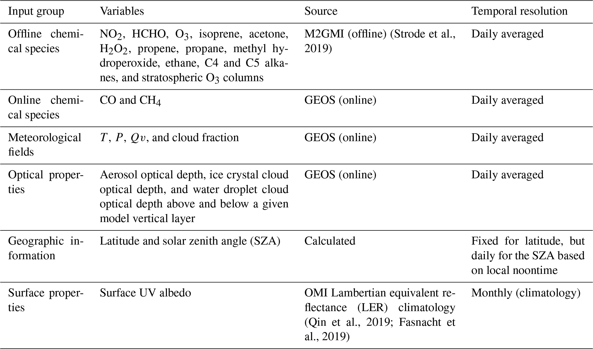
Figure 1 demonstrates the absolute difference in the M2GMI tropospheric NO₂ columns with respect to those of OMI before (a priori) and after (a posteriori) the data fusion application along with AKs in 2005–2019. Inland regions show positive biases over several regions, including central Africa (box A), the US Midwest (box B), and Europe (box C). The same tendency was observed in Anderson et al. (2021). The largest contributors to NO₂ in box A and box C are biomass burning activities (Jaeglé et al., 2005; Giglio et al., 2013), suggesting that either the emission factors or the total burned dry mass were possibly too high in these regions.

M2GMI overestimates NO₂ concentrations in non-urban areas in box B which tend to be more severe during summertime. Although soil NO_x emissions could be the first explanation for this phenomenon, accounting for about 30 % of tropospheric NO₂ columns in the region according to Vinken et al. (2014), the soil NO_x parameterization used in M2GMI relies on Yienger and Levy (1995) and is known to have a low bias (Jaeglé et al., 2005; Hudman et al., 2012; Vinken et al., 2014; Souri et al., 2016). Therefore, there may be other uncertainties in the model concerning the chemistry (e.g., Canty et al., 2015) or area anthropogenic NO_x emissions (Hassler et al., 2016) causing the bias.

Large portions of metropolitan areas in the Middle East, Europe, and the US show an underestimation of NO₂ in M2GMI. Moreover, OMI observations reveal large positive biases over the North China Plain (NCP), a region exhibiting exceptionally high NO₂ levels (e.g., Duncan et al., 2016; Krotkov et al., 2016; Souri et al., 2017). This is primarily because the recent aggressive emission mitigation in China is not accounted for in the bottom-up emission inventory used in the model. We observe several regions over China and the Yellow Sea underestimating NO₂ with respect to OMI observations; this does not improve considerably after the adjustments. This tendency is a result of the use of a fractional error for populating the error covariance matrix a priori, making the prior error too low. Although we used a regularization factor to battle this problem, it did not vary from region to region. A regionally adaptive regularization factor could be a possible remedy for this problem, but at the cost of overcomplicating the interpretation of the results.

As expected, the Bayesian fusion greatly mitigates the regional biases, with notable reductions observed over central Africa, China, the US, the Amazon, and Europe. The regional biases (>80 %) greatly exceed the reported biases associated with the OMI tropospheric NO₂ product (<40 %), suggesting that the adjustments should be considered an improvement. Nonetheless, it is important to acquire an abundance of long-term records from surface spectrometers such as MAX-DOAS and Pandora to comprehensively evaluate the degree of enhancement of M2GMI constrained by OMI within the troposphere, which is currently unavailable for the period of 2005–2019 to the best of our knowledge. The reduction in the biases over remote areas in the tropics is less noteworthy due to large errors in the observations. In other words, it is difficult to have high confidence in the degree of efficiency the model can have in simulating NO₂ over pristine areas by comparing it to OMI. This notion is manifested mathematically in low AKs in remote areas, showing that the rich information from OMI tropospheric NO₂ gravitates more towards polluted regions. This finding assumes that the regularized covariance matrix of the prior error does not vary substantially between the land and ocean and that it is isotropic.

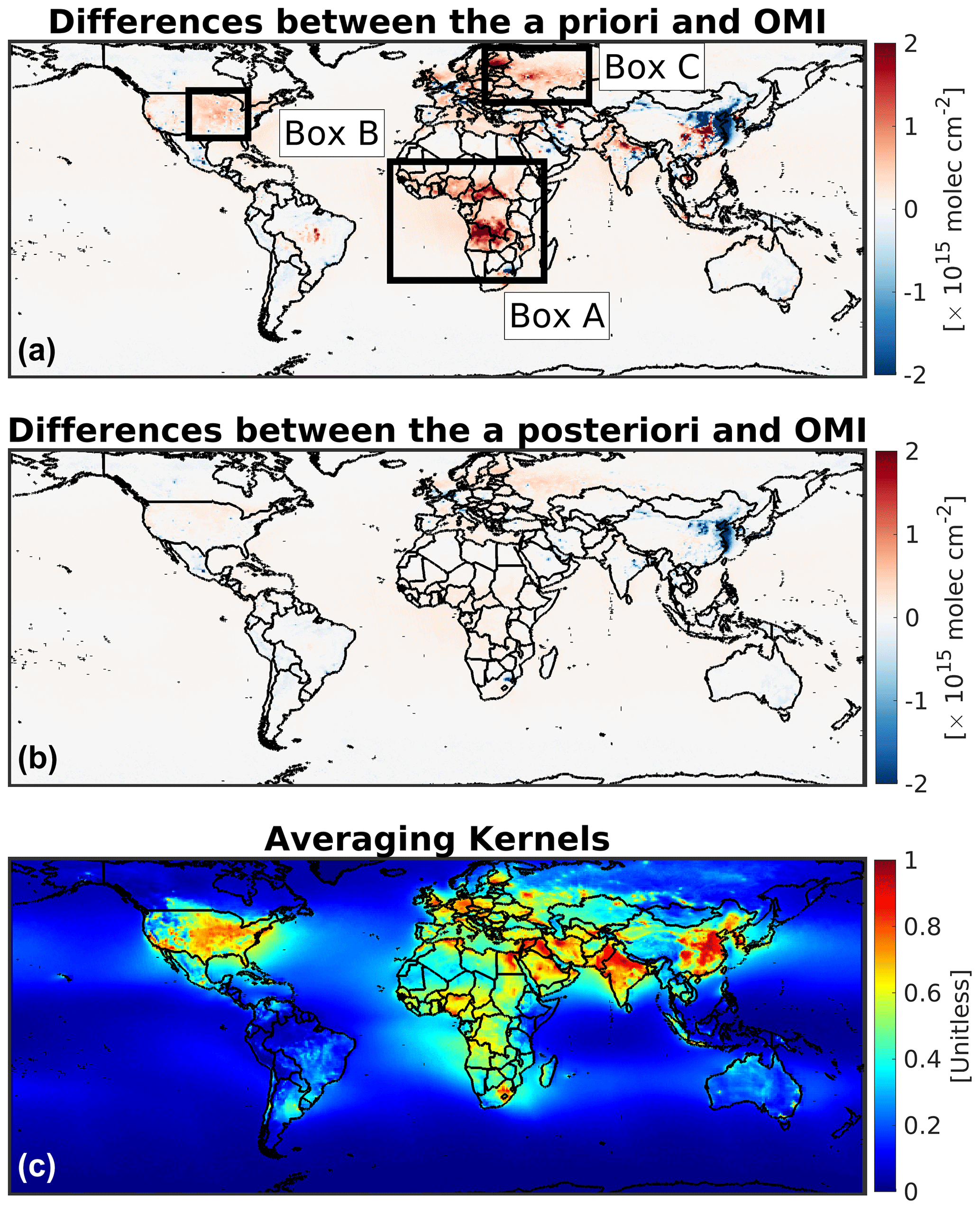
Figure 1 The global maps of the M2GMI tropospheric NO₂ annual difference with respect to those of OMI before (a) and after (b) applying the Bayesian data fusion correction factors in 2005–2019. The mean of the averaging kernels describing the information gained from OMI is shown in panel (c). Grids at high latitudes were removed from the figure due to the too low sample numbers provided by OMI.

Figure 2 illustrates the linear trends of tropospheric NO₂ between 2005 and 2019 observed by OMI and simulated by M2GMI before and after using the OI algorithm. The errors in OMI observations and the constrained M2GMI are considered while calculating the trends. Focusing on the trends of OMI, we observe a consistent picture compared to former studies (Duncan et al., 2016; Choi and Souri, 2015a, b; Krotkov et al., 2016; Jin and Holloway, 2015; Souri et al., 2017). High-income countries, such as the US, those located in western Europe, and Russia (its major cities), have undergone a significant reduction in NO₂ concentrations due to the implementation of emission mitigation regulations. Additionally, low- and medium-income countries, such as those in the Middle East, northern Africa, and India, have seen upward trends in NO₂. Various signs of trends are observed in East Asia. Due to recent effective regulations in China (Zhang et al., 2012), we observe downward trends in the NCP region (Reuter et al., 2014; de Foy et al., 2016; Souri et al., 2017). The downward trend predominantly starting in 2011–2012 counteracts the upward trend in prior years, resulting in statistically insignificant linear trends. Both Japan and South Korea show downward trends during the period of 2005–2019 (Duncan et al., 2016; Souri et al., 2017).

Encouragingly, the prior model simulation of the tropospheric NO₂ trend is consistent with OMI over most of the polluted regions, except for China, where the bottom-up emission inventories used in M2GMI fail to reflect recent mitigation efforts in the NCP region. The posterior estimation has a higher degree of agreement compared to OMI (Sect. S2 in the Supplement). An encouraging observation arising from the comparison of the M2GMI prior and posterior NO₂ trends is the achievement of a higher spatial variance (information) in low- and medium-income countries (e.g., India and Iran). This finding suggests that the emission inventories used in M2GMI lacked adequate spatial information, even at the model spatial resolution.

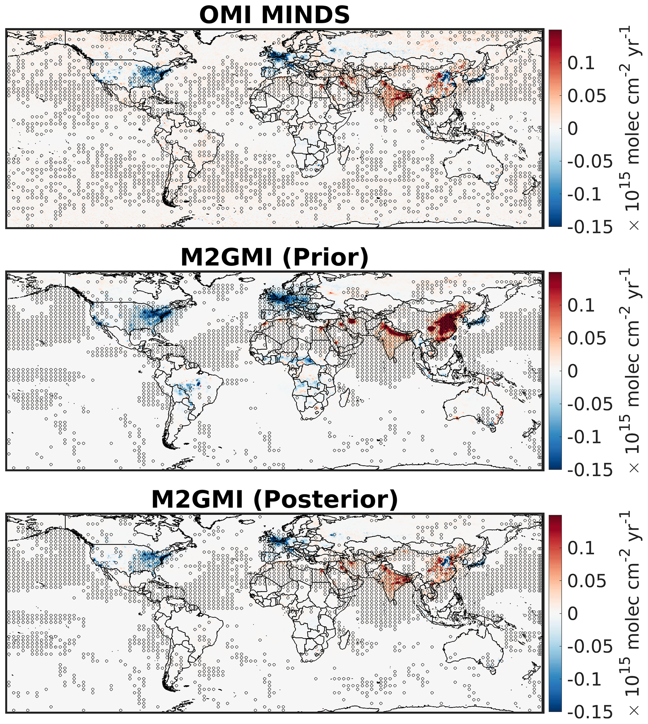
Figure 2 The global maps of linear trends of annual tropospheric NO₂ columns observed by OMI and simulated by M2GMI before and after the Bayesian fusion. The model simulations are sampled at the exact time and location of OMI and are masked if OMI observations were unavailable due to the data quality criteria used. The dots indicate statistically significant trends at the 95 % confidence interval.

3.1.2 Total HCHO columns

We validate the simulated HCHO concentrations, drawing inspiration from the NO₂ comparison framework. Figure 3 illustrates the absolute differences in the simulated HCHO total columns with respect to OMI before and after the Bayesian data fusion application, in addition to AKs. The prior model simulation has considerable skill in capturing the HCHO total columns over several areas, such as the Middle East, Europe, India, and East Asia. However, marked positive biases are discernible in regions with abundant isoprene emissions, such as the Amazon, Southeast Asia, the southeastern US, and central Africa. This outcome is most likely due to an overestimation of biogenic emissions; various investigations have reported a predominantly positive bias (a factor of between 2 and 3) linked to isoprene emissions estimated by MEGAN using satellite measurements in isoprene-rich regions (e.g., Millet et al., 2008; Stavrakou et al., 2009; Marais et al., 2012; Bauwens et al., 2016; Souri et al., 2020a).

The simulated HCHO concentrations are relatively too low over pristine areas, such as high latitudes and mountains. This may be attributed to an underestimation of CH₄ in M2GMI due to assigning its values as background conditions (Strode et al., 2019). The integration of OMI satellite data has proven effective at reducing the biases in areas where HCHO concentrations are large because the signal-to-noise ratio tends to be large, resulting in high AKs. Nonetheless, there are some adjustments over remote areas. In fact, OMI HCHO columns provide more information than OMI NO₂ in remote areas because background HCHO concentrations are not extremely low due to evenly distributed methane and methanol concentrations. It is worth noting that the biases in M2GMI greatly exceed the expected OMI HCHO column biases, suggesting that the adjustments to HCHO improve the model.

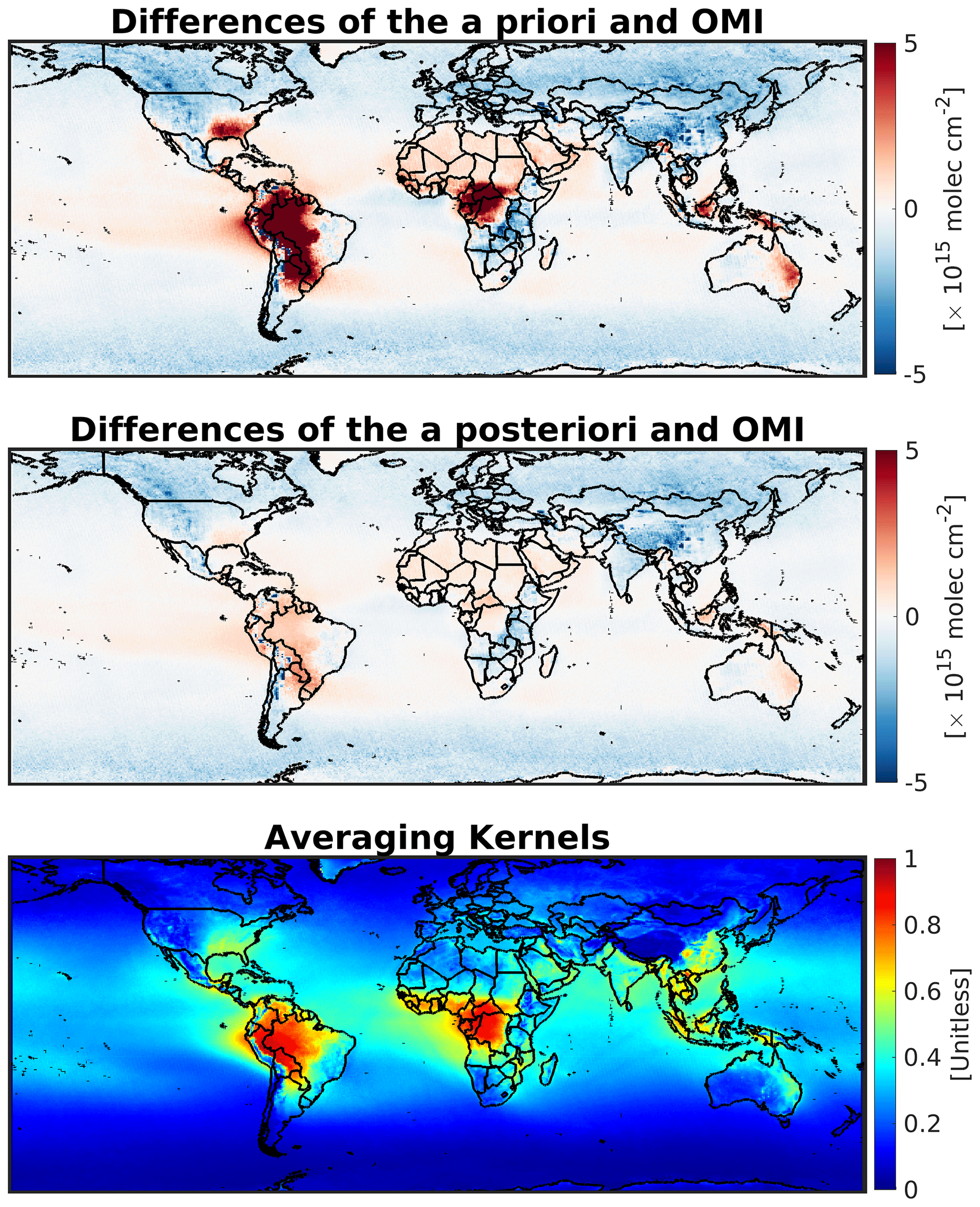
Figure 3 Same as Fig. 1 but for HCHO total columns.

Figure 4 shows the global maps of HCHO total column trends derived from OMI, the prior M2GMI, and the posterior M2GMI. The widespread upward trends in HCHO over India are evident due to a lack of effective efforts to cut emissions related to VOCs (e.g., De Smedt et al., 2015; Kuttippurath et al., 2022; Bauwens et al., 2022). We observe HCHO columns going up in the northwestern US and over oil sands in Canada, possibly due to increased evergreen needleleaf forests and an increase in crude oil production (Zhu et al., 2017), respectively. The downward trends over the southeastern US could be due to a decrease in drought events (Fig. S5 in the Supplement), which significantly affect isoprene emissions and the oxidation of VOCs (Duncan et al., 2009; Naimark et al., 2021; Wang et al., 2022). Alternatively, this downward trend could be partially due to the dampened HCHO production from VOC oxidation due to reduced NO_x emissions (Marais et al., 2012; Wolfe et al., 2016; Souri et al., 2020c). In agreement with previous studies (Stavrakou et al., 2017; Souri et al., 2017, 2020a; Shen et al., 2019), HCHO columns increase over the NCP. HCHO columns tend to decrease over parts of central Africa (e.g., the Democratic Republic of the Congo) and the Amazon basin, potentially due to reduced deforestation rates (De Smedt et al., 2015; Jones et al., 2022). However, large variability in the signs of HCHO trends over these regions is seen: Congo shows an opposite trend to that of the Democratic Republic of the Congo, and the northern portion of the Amazon basin has an increasing trend. Encouragingly, prior knowledge captures the upward trends over India and China along with the downward trends over central Africa. However, the magnitudes and spatial features of these trends are not entirely in line with OMI.

We do not fully understand the HCHO trends over the oceans. Some of these patterns might be caused by transport from nearby sources. For instance, areas around South Asia, South America, and the Gulf of Mexico can be affected by the trends over the land in their vicinity. However, trends over several areas, such as the southern part of the Indian Ocean, Australia, and the Sahara, are not fully explainable by nearby sources. It is possible that certain patterns can be linked to climate variability or OH (Wolfe et al., 2019) affecting the oxidation of background VOCs; in-depth understanding of HCHO trends over the oceans certainly deserves a separate follow-up study.

The posterior estimates line up better with the OMI trends, especially over the Amazon, India, and central Africa (Sect. S3 in the Supplement). The correction factors, however, worsen the trends over the southeastern US and Canada. One possible explanation for this may be the varying errors from the data fusion algorithm, which tend to be reduced more in summertime than in wintertime due to the larger OMI HCHO signal. This results in some degree of inconsistency of the linear trend over these regions, with larger interannual and interdecadal variabilities.

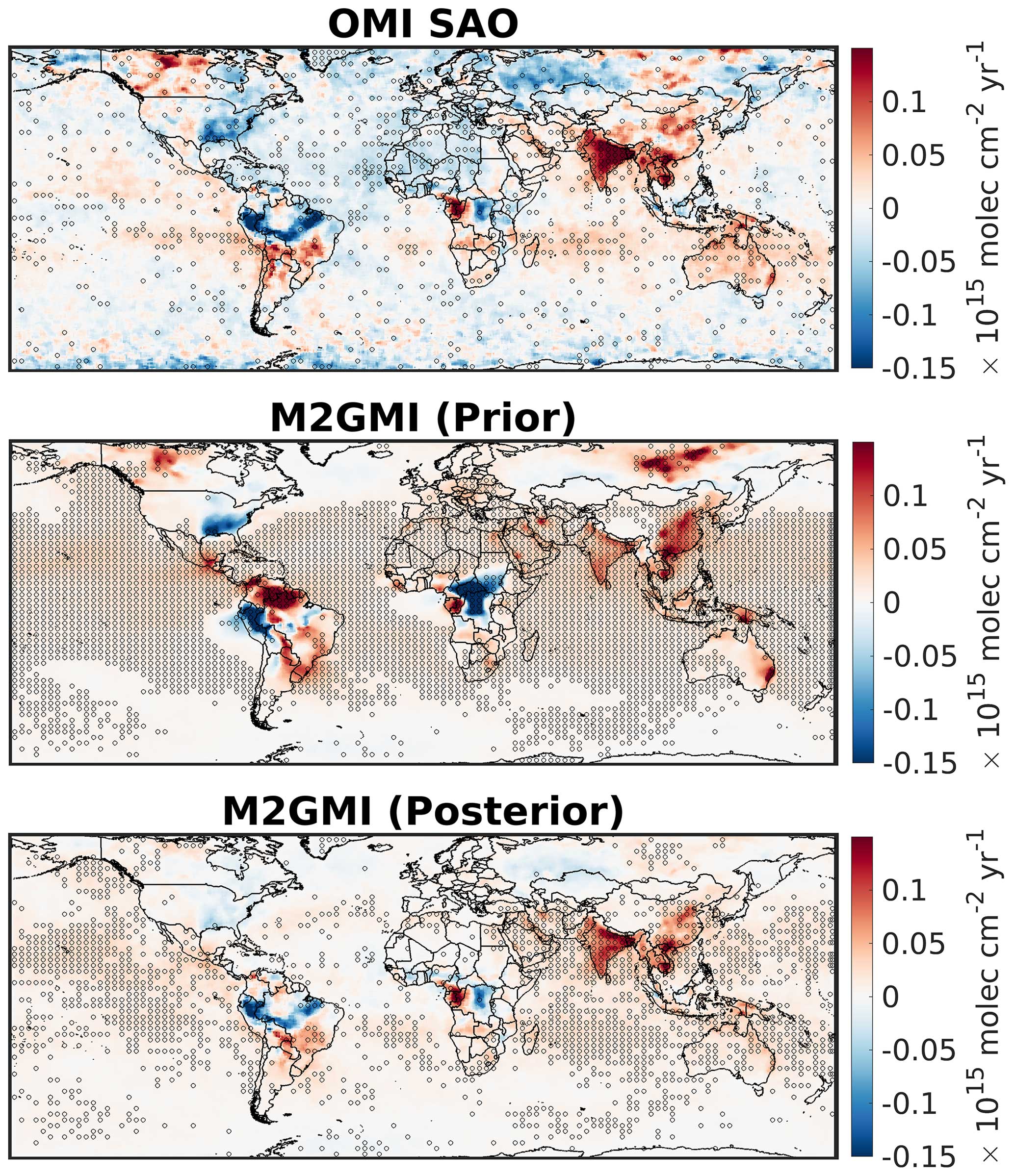
Figure 4 Same as Fig. 2 but for total HCHO columns. The linear trends in OMI SAO are smoothed by a median filter for better visualization.

In summary, we saw that M2GMI NO₂ and HCHO, both inputs to the parameterization of OH, were broadly better presented through the integration of OMI observations. Consequently, the improvement is expected to elevate the level of reliability in the experimental outcomes, particularly in the context of the SOHnitro and SOHform simulations. As for other important compounds, such as stratospheric columns, tropospheric O₃, and water vapor, the comparison of the model with OMI total ozone columns shows a strong degree of agreement (<4 % biases), with no significant trend at the low to middle latitudes (Figs. S1 and S2). The well-documented upward trend in tropospheric ozone in the Northern Hemisphere is well reproduced by M2GMI (Fig. S3). We did not validate GEOS water vapor simulations because of the use of MERRA-2, which is thoroughly validated in Bosilovich et al. (2017). Furthermore, the comparison of integrated water vapor linear trends from our GEOS-5 run (2005–2019) with the satellite data presented in Borger et al. (2022) shows remarkable agreement (Figs. S7–S8).

3.2 Added value of OMI to simulated tropospheric OH

Here, we present the results from three OMI-related experiments (SOMInitro, SOMIform, and SOMInitroform) to understand the effect of OMI adjustments made to M2GMI on TOH. Moreover, we calculate the response of TOH to NO₂ and HCHO using Eq. (5).

Figure 5 consists of three columns, illustrating the percentage adjustments made by OMI NO₂ using OI, the response of TOH to NO₂ concentrations, and the simulated TOH derived from the SOMInitro experiment. The observed pattern of increments aligns with the improvements seen in Fig. 1, with positive (negative) values indicating underestimation (overestimation) of M2GMI. Broadly, the overestimations dominate the underestimations, resulting in a global tropospheric NO₂ reduction of ∼4 %. Upon segregating the increments into four distinct seasons, it becomes evident that the adjustments do not uniformly apply to every season. This non-uniformity is primarily attributed to biases in M2GMI influenced by biomass burning (boxes A and C) (Sect. 3.1.1), both of which exhibit strong seasonality.

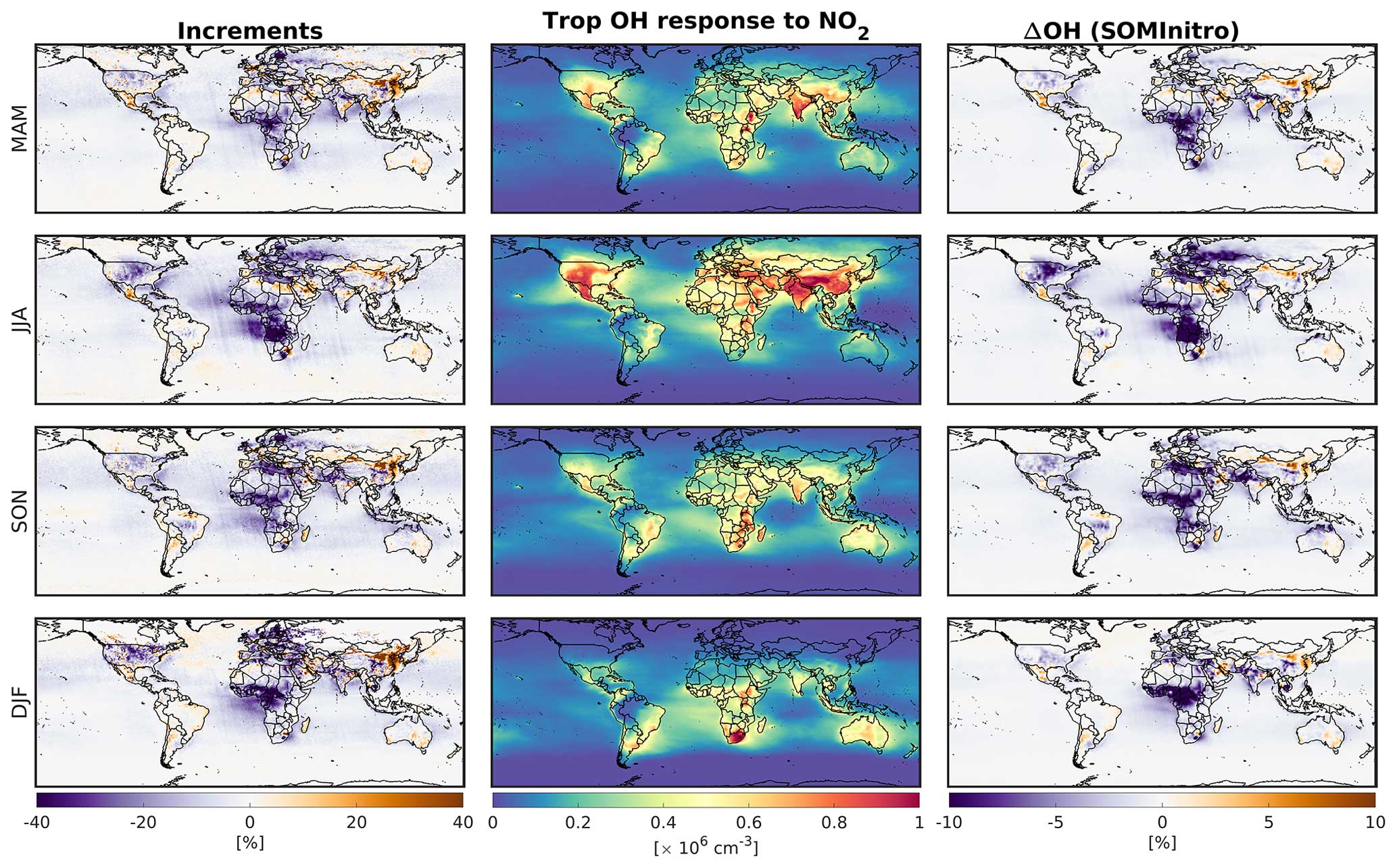
Figure 5 The percentage of the adjustments applied to M2GMI NO₂ fields within the troposphere suggested by OMI tropospheric NO₂ columns for four different seasons (first column), the semi-normalized response of tropospheric OH to tropospheric NO₂ changes based on ECCOH offline calculations (second column), and the resulting effect of the adjustments on the tropospheric OH derived from the online simulation (SOMInitro) (third column). MAM, JJA, SON, and DJF are abbreviations for March–April–May, June–July–August, September–October–November, and December–January–February.

Deciphering the precise chemical processes influencing the response of OH to NO₂ using a machine learning approach is challenging. However, it is widely recognized that reactive nitrogen has a positive feedback on tropospheric OH through increased NO + HO₂ and ozone (Murray et al., 2021; Zhao et al., 2020; He et al., 2021). Considering NO₂ to be a surrogate for reactive nitrogen, similar tendencies are expected, as is evident from the positive numbers from the sensitivity results obtained from offline calculations. The response of TOH to NO₂ displays a pronounced seasonal cycle stemming mainly from photochemistry. It is believed to have some negative values for the sensitivity of OH to NO₂ for extremely polluted regions due to radical termination through NO₂ + OH or ozone titration (Nicely et al., 2018). While we have not identified any negative values in the tropospheric domain, we have observed significant negative values of OH when perturbing NO₂ at the model surface layer (Fig. S26 in the Supplement). This tendency highlights ECCOH's ability to account for nonlinearities.

The impact of adjustments made by OMI NO₂ on TOH is most substantial over regions where both the adjustments and TOH responses to NO₂ are significant. For instance, the large adjustments made over Europe in December–January–February (DJF) do not substantially affect TOH because the response value is low due to reduced photochemistry.

On a global scale, changes to TOH are much milder (1 % reduction) than those occurring regionally. For instance, we see substantial regional impacts (up to 20 %) over many areas, such as central Africa, the US Midwest, the Middle East, and eastern Europe. In light of the global reduction in OH, we observe global column average methane mixing ratios (XCH₄) increasing by 10 ppbv on average (Sect. S4 in the Supplement). This augmentation happens monotonically with an increase of 0.9 ppbv yr⁻¹, ultimately resulting in a ∼15 ppbv difference at the end of the simulation (Fig. S13 in the Supplement). This is essentially due to the long lifetime of CH₄. Likewise, the TOH reduction results in column average CO mixing ratio (XCO) enhancements which transpire more locally than XCH₄ does due to the shorter XCO lifetime. The XCO enhancements reach above 10 ppbv in Africa (Sect. S5).

Figure 6 demonstrates the same scheme as Fig. 5 but with a focus on SOMIform. Marked negative increments are found in regions characterized by elevated isoprene concentrations because of the overestimations of M2GMI biogenic isoprene emissions. Positive increments are mostly confined to high latitudes and certain areas of East Asia (Sect. 3.1.2).

The interplay between HCHO and OH is contingent on the intricate dynamics governing HCHO production from the oxidation of VOCs as well as methane and HCHO loss from various chemical pathways (Valin et al., 2016; Wolfe et al., 2019). In remote areas where HO_x is low, the prevailing sink of HCHO is through photolysis. Conversely, in more polluted areas, the reaction of HCHO + OH emerges as a competing loss pathway. Assuming a steady-state approximation, which is a reasonable assumption for pristine areas, the photolysis loss of HCHO dominates over the reaction with OH, resulting in a linear relationship between HCHO and OH. In other words, high (low) HCHO concentrations are indicative of high (low) TOH. It is because of this that we use HCHO as a proxy of TOH in remote ocean regions. In regions characterized by heightened HO_x levels, OH and HCHO become decoupled. Encouragingly, our implicit parameterization of OH has considerable skill in elucidating these intricate chemical tendencies; specifically, it reveals muted responses in regions with relatively tangible pollution levels, whereas positive responses are evident in ocean regions. Like the results obtained for NO₂, the response map has a seasonal cycle due to photochemistry.

Because of the muted response of TOH to HCHO over land, a substantial portion of geographical regions undergoing significant adjustments made by OMI becomes less important. TOH primarily changes over oceanic areas in a way that it decreases at low latitudes but increases at high latitudes. The largest reduction occurs downwind in the Amazon, where both increments and responses display large magnitudes. As a result of these changes, we see a marginal increase in XCH₄ over the tropics, where OMI increments reduced TOH. The HCHO adjustment did not noticeably affect XCO either (Sect. S5).

Modifications of HCHO by OMI do not signal substantial changes in background VOC oxidation through OH. In fact, TOH changes by this proxy are 1 order of magnitude less than those by OMI NO₂. This tendency is a result of two key factors: (i) the adjustments wield their major influence over the oceans, where M2GMI has a fair performance; and (ii) the amount of information obtained from OMI HCHO (i.e., AKs) remains somewhat limited in remote areas due to low signal-to-noise ratios.

Due to the rather independent nature of the TOH responses to NO₂ and HCHO, where the former prevails over land and the latter over ocean, the concurrent adjustments of HCHO and NO₂ using OMI (i.e., SOMInitroform) result in a rather linear combination of outcomes derived from SOMIform and SOMInitro (Fig. S21 in the Supplement). This linear outcome is characterized by a large decrease in TOH at low latitudes and a moderate increase at high latitudes, resulting in a decrease in global TOH of ∼1 %.

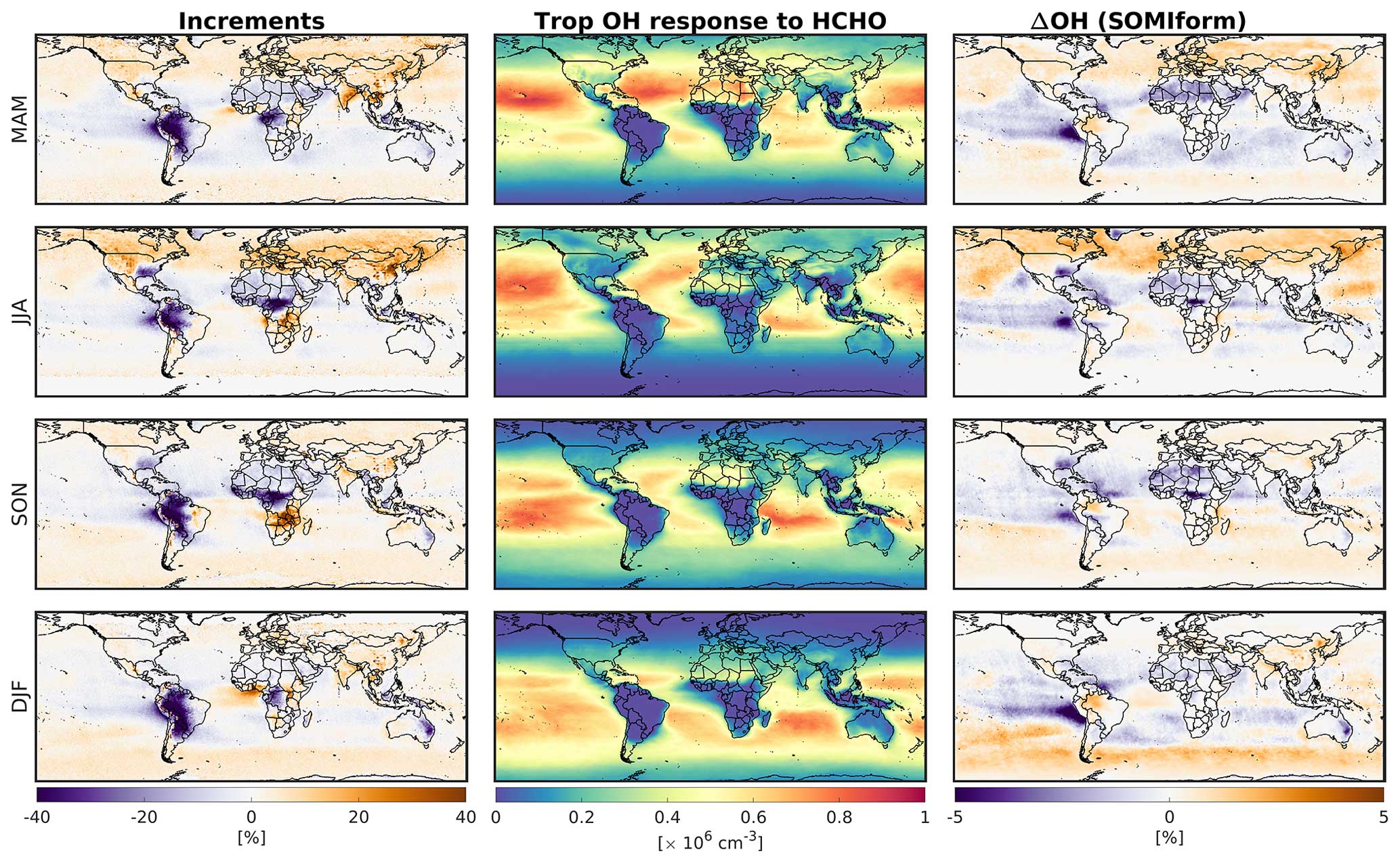
Figure 6 Same as Fig. 5 but for HCHO.

3.3 Synergy of the model and satellite observations for explaining TOH long-term trends

3.3.1 The dominant contributor to TOH trends

Here, we take advantage of the wealth of information from satellites and our well-characterized model used for the inputs to the parameterization of OH to rank the dominant contributor to TOH linear trends. By assuming that TOH follows a linear combination of each individual experiment designed to isolate OH drivers and proxies (i.e., SOHnitro, SOHform, SOHtropozone, SOHstratozone, and SOHwv), wherein second-order (or higher-order) chemical feedback is disregarded, we can determine the biggest contributor to the TOH trend for each model grid box by finding which driver or proxy holds the largest absolute amount. We only label a grid if the absolute linear trend of the dominant driver or proxy surpasses the second most dominant one by 30 %.

Figure 7 illustrates the dominant factor explaining TOH trends. Several patterns can be found from this result. (i) NO₂ plays a significant role in TOH trends in various polluted areas, such as Asia and the Middle East. (ii) The upward trend of TOH over the western Pacific Ocean is primarily attributed to increased tropospheric ozone from Asia (e.g., Lin et al., 2017); also, we observe a significant fraction of TOH over the tropical Atlantic Ocean, increasing because of rising tropospheric ozone from Africa, Central America, and South America (Edwards et al., 2003). (iii) HCHO is convolved with TOH trends over the tropical oceans. (iv) Water vapor plays a pivotal role in shaping TOH trends over the oceans across the globe. (iv) Stratospheric ozone columns are mostly significant over the South Pole due to the ozone healing process (Fig. S2). The next sections will focus on the magnitudes of these trends and the degree to which they can collectively explain the variance in TOH trends compared to Sanalysis.

It is important to recognize that the analysis presented here should be interpreted as a relative assessment of a limited number of TOH drivers and proxies, rather than as an exhaustive evaluation of all the physical and chemical processes that are tied to TOH. Nonetheless, the data presented offer valuable insights into the TOH trends and can be used as a basis for further research.

Figure 7 The major contributor to TOH trends based on the largest absolute trends of TOH drivers and proxies above 30 % of the second most dominant factor.

3.3.2 Magnitudes of linear trends of TOH key inputs

Figure 8 shows the TOH linear trends influenced by NO₂ (SOHnitro), HCHO (SOHform), water vapor (SOHwv), tropospheric ozone (SOHtropozone), and stratospheric ozone (SOHstratozone). Discussions of each parameter follow.

• SOHnitro – the trends in TOH driven by NO₂ show a strong correlation with the a posteriori trend discussed in Sect. 3.1.1, with low- and medium-income countries experiencing an increase in TOH due to rising NO₂ levels, while high-income countries see a reduction in TOH due to the opposite trend. The most significant increase in TOH is observed over India, where both the NO₂ trend and the TOH sensitivity to NO₂ are prominent. The most rapid regional decline in TOH seems to be over the NCP because of NO_x reductions that began after 2011. This finding is particularly noteworthy since M2GMI did not reproduce this trend without OMI as a constraint. The trend in TOH resulting from NO₂ is predominantly anthropogenic in nature. This aligns with the findings of Chua et al. (2023), who observed that the impact of lightning NO_x emissions on TOH trends was relatively minor. The global trend in TOH driven by NO₂ is positive but with considerable variation due to the significant disparities in how anthropogenic NO_x emissions have changed.

• SOHform – we saw that HCHO was a reasonable proxy for TOH over the oceans. Accordingly, the TOH trends are primarily observed over the oceans, especially over the Pacific and Indian oceans. This lines up with the information gathered from the analysis of M2GMI and OMI HCHO observations (Fig. 4). These upward HCHO trends, as discussed in Sect. 3.1.2, may be influenced by transport and dynamics. It is worth noting that the increase in TOH tied to this proxy (HCHO) is a global tendency attributable to the relatively uniform rise in HCHO levels across the oceans.

• SOHwv – water vapor is a primary source of OH. The offline sensitivity of ECCOH captures this tendency (Fig. S22 in the Supplement). Accordingly, the TOH linear trends mirror those of integrated water vapor (IWV) (Fig. S8), with major increases over the oceans. Similar to the other experiments, the global TOH increases because of rising water vapor in the atmosphere. We acknowledge that understanding the reasons for changes in water vapor, which our model shows to agree with Borger et al. (2022), is a complex subject that goes beyond the scope of our research. It requires an in-depth understanding of the water cycle, evapotranspiration and precipitation rates, and the effect of temperature on the air's capacity to hold moisture, known as the Clausius–Clapeyron relationship. However, a great deal of effort has been made to demonstrate that global water vapor levels have increased significantly in recent decades. This is based on reanalysis data, microwave satellites, and in situ measurements (Trenberth et al., 2005; Chen and Liu, 2016; Wang and Liu, 2020; Allan et al., 2022), which is consistent with what our model shows, as it is well constrained by MERRA-2 data.

• SOHtropozone – the impact of tropospheric ozone on OH formation is widely acknowledged (Lelieveld et al., 2016). Likewise, our ECCOH offline sensitivity tests have revealed a largely positive correlation between tropospheric ozone and OH (Fig. S23 in the Supplement). Consequently, the linear trends observed in TOH closely mirror those of tropospheric ozone in M2GMI (Fig. S3). This tendency is especially noticeable in the Atlantic Ocean, East and Southeast Asia, as well as the northern region of the Pacific Ocean, where rising ozone levels have increased TOH. M2GMI suggests that tropospheric ozone levels in the Southern Hemisphere have decreased (Sect. S1), potentially leading to a downward trend in TOH, an observation that has yet to be fully confirmed (e.g., Thompson et al., 2021). This finding is especially important given past research indicating that models tend to exaggerate TOH asymmetry between the Northern Hemisphere and the Southern Hemisphere (Strode et al., 2015; Naik et al., 2013). The decrease in the simulated tropospheric ozone may offer a plausible explanation for this tendency, but further verification is deemed necessary. Like the previous experiments, tropospheric ozone on average leads to a global increase in TOH in 2005–2019.

• SOHstratozone – stratospheric ozone columns reduce UV actinic fluxes, leading to a reduction in tropospheric JO¹D and thus OH, a tendency well reproduced by ECCOH (Fig. S24 in the Supplement). Nonetheless, stratospheric columns did not change noticeably in the tropics and at the middle latitudes, where OH production is important. Consequently, the linear trends are close to zero or faintly negative due to a slight upward trend in the column. This tendency results in a rather uniform decrease in TOH globally.

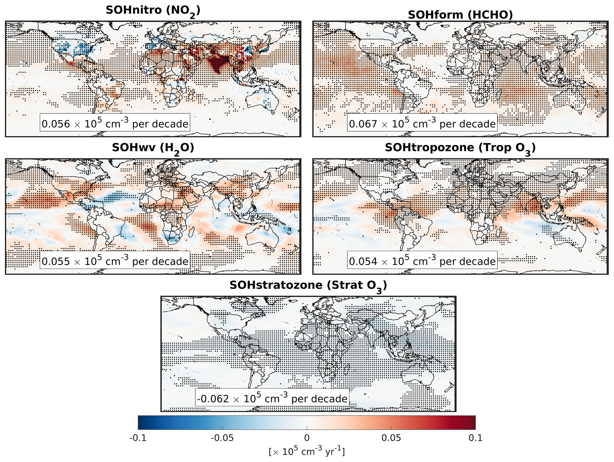
Figure 8 The contribution of each TOH key input (addressed in this study) to TOH in 2005–2019. HCHO, NO₂, and water vapor results are observationally constrained. Stratospheric ozone columns yielded comparable results compared to the total ozone columns observed by OMI. However, a large portion of the tropospheric ozone trend has remained unverified in the Southern Hemisphere. ENSO affects the variability of TOH (Anderson et al., 2021), so we add a linear term to Eq. (4) that is a function of the Niño 3.4 Index. This helps prevent ENSO from affecting the subsequent results. Dots indicate the statistically significant trends.

3.3.3 OMI contributions to TOH trends

It is attractive to gauge the additional information gained from OMI to better represent the linear trends of TOH. To achieve this, we need to analyze three sets of model output: one with OMI scaling factors, one without OMI scaling factors, and one with the NO₂ and HCHO drivers (i.e., SOHnitro and SOHform). The linear trends from these sets of model results are shown in Fig. 9. The trends in the first column illustrate the overall effect of NO₂ and HCHO on TOH trends, while the other two subplots isolate the effect of OMI from the prior information based on M2GMI. M2GMI plays a significant role in shaping the trends in SOHnitro, possibly due to the small discrepancy between the trends in OMI and M2GMI columns over regions where TOH is responsive to the driver. The most significant impact of OMI on NO₂ is visible over the NCP. Concerning HCHO, OMI slows down the upward trends in TOH over the oceans, which was suggested by M2GMI. In general, M2GMI largely dictates the overall shape of TOH trends driven by NO₂ and HCHO, possibly due to the small difference between the model and OMI observations and/or the limited informational content in OMI.

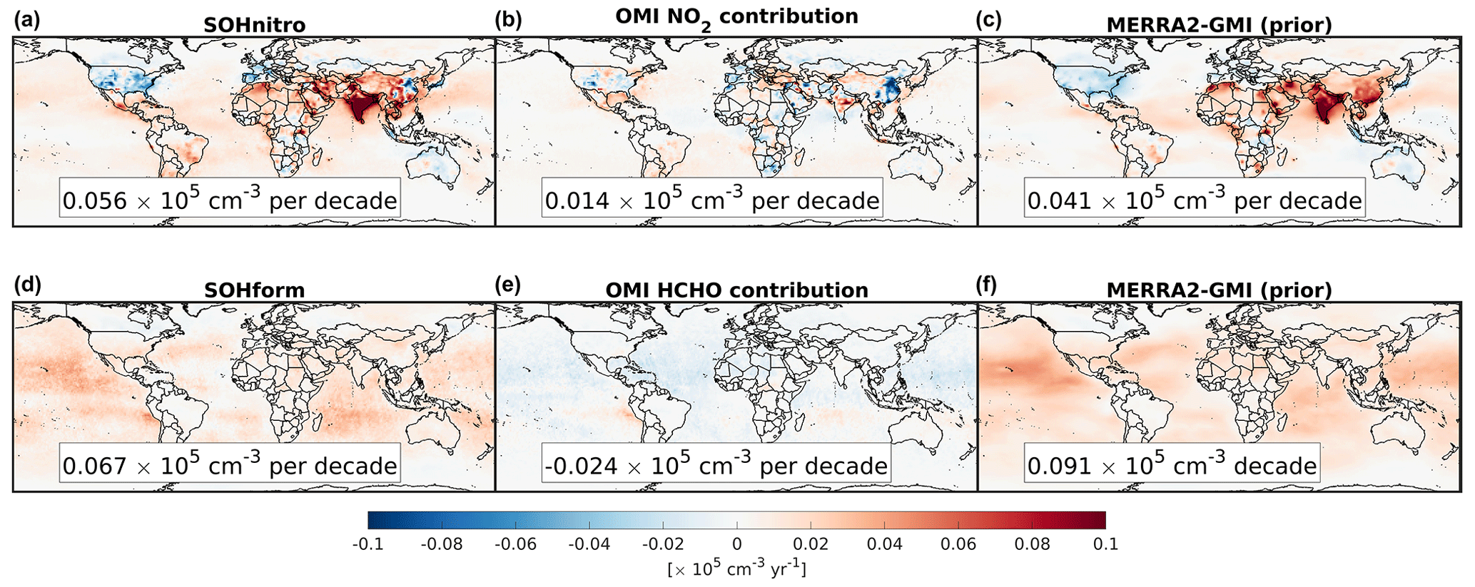
Figure 9 The resulting effect of tropospheric NO₂ and HCHO on TOH linear trends during 2005–2019 (a, d). The contributions of OMI information added on top of the prior knowledge (M2GMI) (b, e). The effect of the prior knowledge on shaping TOH linear trends (c, f).

3.3.4 How well can these experiments explain the simulated trends collectively?

We find that there is a good degree of correlation between the sum of the linear trends and those of Sanalysis (R²=0.65), indicating that a good portion of the variability in the TOH trend can be explained well by these experiments (Fig. S25 in the Supplement). Figure 10a shows the linear trend of TOH from Sanalysis in 2005–2019, and Fig. 10b shows the sum of the linear trends of the five OH key inputs. These maps are one of the most recent and detailed TOH trends available, relative to newer studies (Nicely et al., 2018; Zhao et al., 2020; Chua et al., 2023). The TOH trend from Sanalysis varies greatly, where positive values are prevalent over the northern parts of the Pacific Ocean, the Middle East, central Africa, and several regions over East Asia. Negative trends are found over the US, Southeast Asia, and the southern part of the Pacific Ocean. The linear sum of the experiments strongly aligns with Sanalysis, particularly over the Northern Hemisphere, emphasizing that the selected parameters are sensible choices for reproducing a large portion of the variance in the TOH trend.

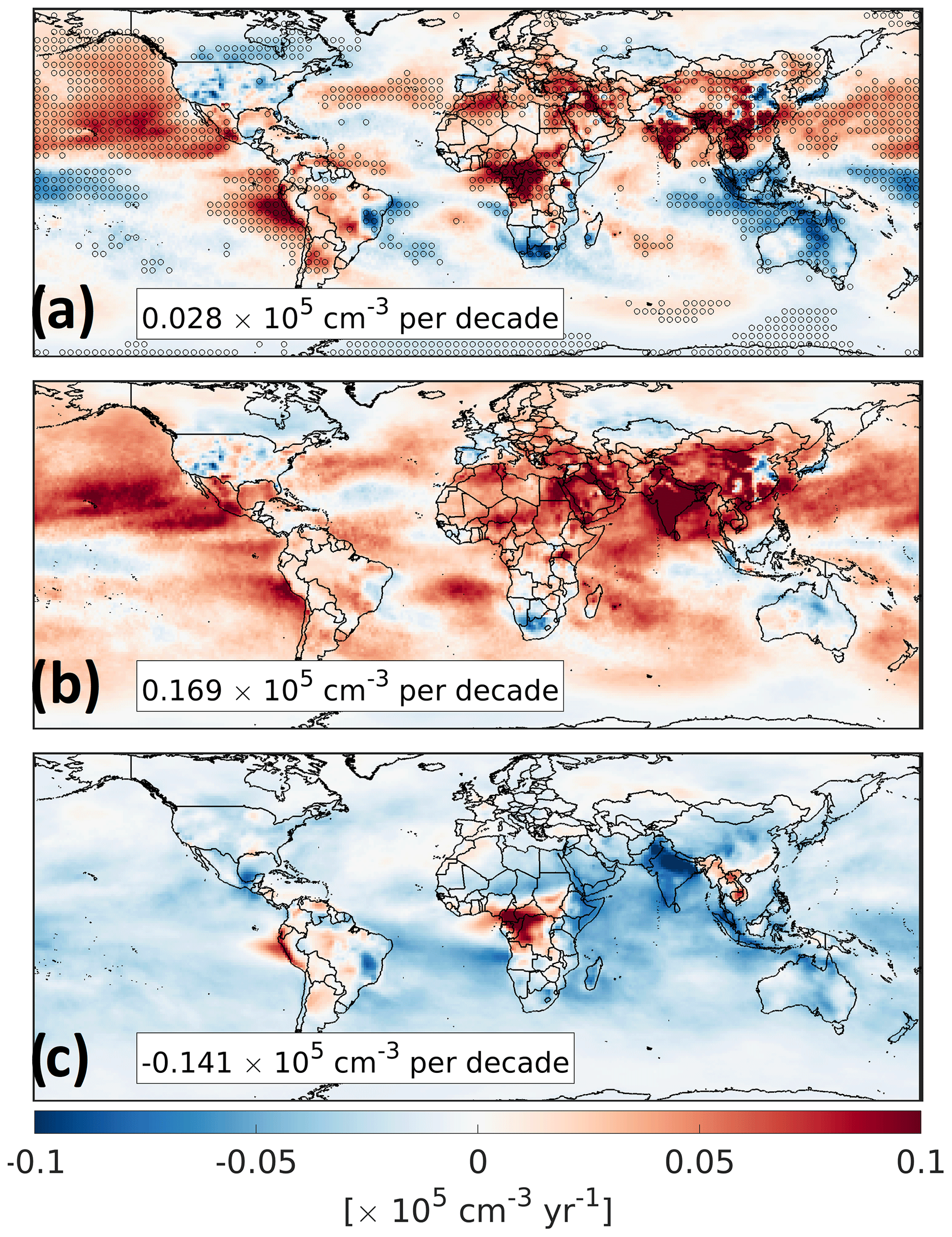
Figure 10 (a) The linear trends derived from the Sanalysis experiment, the “best effort” to simulate the evolution of the CH₄–CO–OH cycle, from 2005 to 2019. The statistically significant trends are superimposed by dots. (b) The linear summation of the five selected TOH influences, i.e., water vapor, NO₂, HCHO, and stratospheric and tropospheric ozone, showing a strong degree of correspondence to the top panel, particularly in the Northern Hemisphere. (c) The unexplained portion of the TOH trends, which was not explainable by the five experiments addressed in this research.

Revealing the unexplained portion of TOH trends, which cannot be attributed to the selected TOH experiments, is necessary. Within the model, various physiochemical factors such as CO, CH₄, dynamics, aerosols, and clouds can impact the TOH trends. Although we will not delve into these drivers in this study, we can identify unexplained parts of TOH trends by subtracting the sum of trends derived from the five primary TOH key inputs from those of Sanalysis, which discounts second-order (or higher-order) chemical feedbacks. Figure 10c displays the unexplained TOH trends between 2005 and 2019. It is readily apparent that there are uniform and significant downward trends in TOH in the tropics and subtropics, where photochemistry is strong. This is most likely triggered by increasing concentrations of CH₄, which is demonstrated in Fig. S10 in the Supplement, causing OH levels to decrease over time. It is very probable that the extent of these downward trends in TOH has been exaggerated in our model because of the simulated CH₄ increasing too rapidly compared to in situ observations. The overestimation of the upward trend in CH₄ in our model compared to in situ observations could be caused by the biases (∼3 %) in sources minus sinks and/or the initial condition. Consequently, the globally averaged TOH trend derived from Sanalysis may be slower than it should be. Lastly, an unexplained strong upward trend in TOH over central Africa lingers.

4 Conclusions

While a comprehensive multi-sensor or multi-species data assimilation and inverse modeling approach, such as Souri et al. (2020a, 2021) or Miyazaki et al. (2020), would be ideal for fully harnessing the potential of satellite information to improve multiple aspects of a model representing OH, this would be prohibitively expensive. Therefore, our simplified approach serves the purpose of understanding the first-order effects of observational adjustments to TOH drivers and proxies before committing substantial resources to the implementation or execution of an observationally constrained full-chemistry model. Here, we implemented the newest version of the parameterization of OH, following Anderson et al. (2022), within NASA's GEOS model, presenting an opportunity to understand and mitigate TOH biases caused by misrepresentation of HCHO and NO₂ concentrations with respect to the state-of-the-art OMI NO₂ and HCHO retrievals using Bayesian data fusion as well as to unravel the intricacies of TOH in its key inputs, such as tropospheric and stratospheric ozone and water vapor.

We found large positive biases in tropospheric NO₂ columns in M2GMI, the archived model used as an input to the parameterization of OH, compared to OMI over Africa, eastern Europe, and the US Midwest. Because of a large positive effect of NO₂ (a surrogate for NO_x) on TOH, a tendency well captured by our implicit parameterization, these overestimations introduced significant regional biases in TOH of up to 20 % and a global overestimation of TOH of 1 %. Consistent with former work, we saw distinct disparities in the signs of linear trends of tropospheric NO₂ over high- and medium-income countries (i.e., negative) and low-income countries (i.e., positive). While M2GMI generally replicated these trends, notable deviations were identified over China, leading to an erroneous trend of TOH.

Pronounced inaccuracies with regards to both the simulated HCHO magnitude and the trend in M2GMI were revealed by OMI over land. However, this proxy for OH was loosely connected to TOH in areas where photolysis was not the major sink of HCHO (Wolfe et al., 2019), especially over land. Over the oceans, where HCHO and TOH were highly correlated, adjustments to M2GMI by OMI HCHO were relatively mild, resulting in small alterations to TOH which were 1 order of magnitude lower than those of NO₂. These mild alterations speak to either an insufficient amount of information in OMI or the reasonable accuracy of M2GMI over pristine areas.

In general, five variables, i.e., NO₂, HCHO, water vapor, tropospheric ozone, and stratospheric ozone, could collectively account for 65 % of the variance in TOH trends globally. To estimate this, we conducted various modeling experiments to isolate the effects of NO₂, HCHO, water vapor, tropospheric ozone, and stratospheric ozone on long-term trends of TOH in 2005–2019 at 1°×1° resolution. Except for tropospheric ozone, these variables were either constrained by observations or aligned with independent observations, boosting confidence in our trend results. Given the robust positive correlation between OH and NO₂, HCHO, water vapor, and tropospheric ozone over regions where photochemistry was active, TOH trends influenced by these variables closely mirrored the trends in their respective drivers and proxies. For instance, high- and medium-income countries exhibited negative TOH trends driven by NO₂. Rising tropospheric ozone over East and South Asia, heavily vetted by various observations (Gaudel et al., 2018), led to an upswing in TOH over the Pacific Ocean. The trend of water vapor, greatly in agreement with independent observations (Borger et al., 2022), was dominantly positive over the oceans, leading to further enhancement of TOH. The rising HCHO over the Pacific and Indian oceans suggested by the constrained M2GMI was associated with increased TOH. The effect of stratospheric ozone on TOH was marginal at the low and middle latitudes due to negligible changes in stratospheric ozone columns in M2GMI, reconfirmed by OMI total ozone column observations.

A large offset between our analysis experiment with varying CO and CH₄ concentrations was observed after removing the sum of the linear trends derived from these five key experiments from the analysis experiment, indicating that our future research using ECCOH should include new experiments isolating the effects of CO, CH₄, and transport (e.g., Gaubert et al., 2017; Zhao et al., 2020). Those experiments will refine the investigation of the unexplained portion of the TOH trend.

The development of an effective parameterization of OH that is capable of integrating advanced satellite-based gas retrievals and improved weather forecast models enabled us to unravel the convoluted response of TOH to various parameters. Nonetheless, it is important to recognize some of the limitations associated with our work: first, the offline nature of the Bayesian data fusion algorithm makes the entire experiment blind to the interconnected responses of various compounds, such as ozone or aerosols, and to adjustments to NO₂ and HCHO. Despite this limitation, our work has provided valuable insights into the first-order effects of adjustments on TOH key inputs. This can help quickly identify areas where our prior knowledge is least reliable for simulating TOH. Second, the machine learning algorithm employed for parameterizing OH is implicit and its response to drivers and proxies is complex, making it difficult to quantitatively verify against full chemistry models. However, by including a vast number of parameters in the parameterization, Anderson et al. (2022) boosted the ability to understand the convoluted chemistry of OH. This has allowed for reproduction of OH for events not included in the training dataset (Anderson et al., 2022, 2023, 2024).

The longevity and stability of Aura's record of observations have played a significant role in constraining and assessing several important variables pertaining to TOH on a global scale. This is exemplified by the wealth of information obtained from OMI NO₂, HCHO, water vapor, total ozone columns, and Microwave Limb Sounder (MLS) temperature and ozone, which are used directly or indirectly in our analysis. However, as Aura's mission comes to an end, there will be a gap in the monitoring of these variables. TROPOMI, OMI's successor, can help fill this gap, but its record of observation is still short; therefore, it is important to invest in research to harmonize data from multiple satellite observations such as OMI and TROPOMI (e.g., Hilboll et al., 2013). This is because each sensor can have different biases and spatial representativities, which can lead to inconsistencies and potentially conflicting values if they are used together.