Aerosol–meteorology feedback diminishes the transboundary transport of black carbon into the Tibetan Plateau

Black carbon (BC) exerts potential effects on climate, especially in the Tibetan Plateau (TP), where the cryosphere and environment are very sensitive to climate change. The TP saw a record-breaking aerosol pollution event during the period from 20 April to 10 May 2016. This paper investigates the meteorological causes of the severe aerosol pollution event, the transboundary transport flux of BC, the aerosol–meteorology feedback, and its effect on the transboundary transport flux of BC during the severe aerosol pollution event using observational and reanalysis datasets as well as simulation based on a coupled meteorology and aerosol/chemistry model, Weather Research and Forecasting model coupled with Chemistry (WRF-Chem). By analyzing weather maps derived from the reanalysis dataset, it is found that the plateau vortex and southerly winds were key factors that contributed to the severe aerosol pollution event. Subsequently, due to the good performance of the WRF-Chem model for the spatiotemporal characteristics of meteorological conditions and aerosols, the transboundary transport flux of BC during the pollution event was investigated. The results show that the vertically integrated cross-Himalayan transport flux of BC decreases from west to east, with the largest transport flux of 20.8 mg m⁻² s⁻¹ occurring at the deepest mountain valley in southwestern TP. Results from simulations with and without aerosol–meteorology feedback show that aerosols induce significant changes in meteorological conditions in the southern TP and the Indo-Gangetic Plain (IGP), with the atmospheric stratification being more stable and the planetary boundary layer height decreasing in both regions, and the 10 m wind speed increasing in the southern TP but decreasing in the IGP. Changes in meteorological conditions in turn lead to a decrease in the surface BC concentration in the southern TP of up to 0.16 µg m⁻³ (50 %) and an increase in the surface BC concentration in the IGP of up to 2.2 µg m⁻³ (75 %). In addition, it is found that the aerosol–meteorology feedback decreases the vertically integrated transboundary transport flux of BC from the central and western Himalayas towards the TP. This study not only provides crucial policy implications for mitigating glacier melt caused by aerosols over the TP but is also of great significance for the protection of the ecological environment of the TP.

1 Introduction

Known as “the Third Pole”, the Tibetan Plateau (TP) plays a significant role in driving climate change in the Northern Hemisphere and even the globe through thermal and dynamical forcing (Wu et al., 2007; Lau et al., 2006). Also, since it has the most concentrated glacier and snow cover outside of the polar regions, the TP supplies a substantial portion of the water demand for almost 2 billion people (Yao et al., 2022). However, numerous studies in recent years have reported that the TP has experienced significant and rapid climate warming during the last few decades (Kang et al., 2010; You et al., 2016, 2021). As a result of this intensive warming, glaciers over the TP have undergone unprecedented widespread losses and accelerated retreats (Kang et al., 2010; Yao et al., 2007). Besides high levels of greenhouse gases (Duan et al., 2006), other factors like atmospheric heating and the reduction in the albedo of the snow also contribute significantly to this climate warming and glacier retreat (Xu et al., 2009; Zhang et al., 2021; Kang et al., 2019b). However, with an average elevation exceeding 4 km, the TP is relatively undisturbed by human activities and is one of the most pristine regions on the earth. Hence, aerosols over the TP are mainly sourced from surrounding regions (Kang et al., 2019b). In particular, with nearly half of the world's population and heavy industry, South and East Asia, which are adjacent to the TP, are the world's hotspots for aerosol pollution (Lelieveld et al., 2016). Driven by atmospheric circulation, aerosols from South and East Asia can be transported to the TP, where they exert a striking effect on the hydrological cycle and climate (Wu et al., 2008; Ramanathan et al., 2005; Liu et al., 2014). Previous studies indicated that aerosols over the TP are primarily transported via typical long-distance transboundary transport events (Kang et al., 2019a). It is therefore of paramount importance to excavate the meteorological causes of the severe aerosol pollution event as well as the transboundary transport flux of aerosols during that event.

Black carbon (BC) exerts a substantial impact on climate through several mechanisms, including by heating the atmosphere by absorbing shortwave and longwave radiation, by darkening the surface of snow and ice and thus accelerating the melt of the cryosphere, and by modifying the optical and microphysical properties of clouds (Kang et al., 2019b; Ramanathan and Carmichael, 2008; Flanner et al., 2007; Skiles et al., 2018). An estimation reported in the literature shows that BC is the second most important type of human forcing after carbon dioxide, with a global climate forcing of 1.2 W m⁻² (Ramanathan and Carmichael, 2008; Chung et al., 2005). Moreover, the radiative forcing of BC in snow and ice is approximately twice as high as that of carbon dioxide and other types of anthropogenic forcing (Flanner et al., 2007; Qian et al., 2011; Hansen and Nazarenko, 2004). In particular, as it is an area that is sensitive to global climate change, the TP has experienced an increase in BC content in recent years (Xu et al., 2009). There is no doubt that BC plays a substantial role in the climate and environmental changes over the TP. However, previous studies primarily focused on the origin of BC and its effect on climate over the TP on annual and seasonal timescales (Yang et al., 2018; Hu et al., 2022b; Rai et al., 2022). The transboundary transport flux of BC towards the TP during the severe aerosol pollution event on the synoptic scale is still unknown, so it should be studied urgently.

Severe aerosol pollution events are usually accompanied by complex aerosol–meteorology feedback. Moreover, numerous studies have revealed that the aerosol–meteorology feedback has a substantial effect on the surface aerosol concentration (Wu et al., 2019; Zhang et al., 2018b; Zhao et al., 2017; Hong et al., 2020; L. Chen et al., 2019; Gao et al., 2016). For instance, some studies have analyzed the aerosol–meteorology feedback and its effect on the surface PM_2.5 concentration during heavy aerosol pollution events in winter in northern China, and they found that positive aerosol–meteorology feedback can increase the surface PM_2.5 concentration (Li et al., 2020; Qiu et al., 2017; Wu et al., 2019). Nonetheless, other studies suggested that the aerosol–meteorology feedback can reduce the surface PM_2.5 concentration in Beijing (Zheng et al., 2015; Gao et al., 2016). Based on in situ observational data, Zhong et al. (2018) analyzed the aerosol–meteorology feedback during several air pollution events in Beijing and concluded that 70 % of the increase in the surface PM_2.5 concentration in the cumulative outbreak stage of haze could be attributed to the aerosol–meteorology feedback. The abovementioned studies mainly focused on the economically developed central and eastern China regions. However, the TP has a very high altitude and complex topography along with a tough environment and scarce in situ observational data. Systematic and comprehensive studies on the aerosol–meteorology feedback in this region are still lacking and this feedback needs urgent investigation. As studies related to the aerosol–meteorology feedback involve sensitivity tests, numerical simulation is the best way to realize the relevant research. In addition, a study conducted by Huang et al. (2020) indicates that the aerosol–meteorology interaction and feedback enhanced the transboundary transport of pollutants between the North China Plain and the Yangzi River Delta regions and thus exacerbated the haze levels in these two regions simultaneously. For the Third Pole region, the effect of the aerosol–meteorology feedback on the transboundary transport flux of BC remains unclear, and this is worth an in-depth study. Therefore, in this study, we attempt to investigate the meteorological causes of the severe aerosol pollution event, the transboundary transport flux of BC, the aerosol–meteorology feedback, and its effect on the transboundary transport flux of BC during the severe aerosol pollution event using observational and reanalysis datasets as well as numerical simulation with an advanced regional climate-chemistry model, Weather Research and Forecasting model coupled with Chemistry (WRF-Chem). This study not only provides crucial policy implications for mitigating glacier melt over the TP; it is also of great significance for the protection of the ecological environment of the TP.

The structure of this paper is organized as follows. Following the “Introduction”, data, the definition of an aerosol pollution event, and the WRF-Chem model configuration and experimental design are described in Sect. 2. In Sect. 3, the meteorological causes of the severe aerosol pollution event, the transboundary transport flux of BC, the aerosol–meteorology feedback, and its effect on the transboundary transport flux of BC during the severe aerosol pollution event are investigated. Section 4 presents the main conclusions.

2 Data, the definition of a severe aerosol pollution event, WRF-Chem model configuration, emissions, and experimental details

2.1 Data

2.1.1 ERA-Interim

To explore the meteorological causes of the severe aerosol pollution event, the geopotential height, air temperature (T), and wind fields at 500 hPa with a horizontal resolution of ${\mathrm{0.05}}^{\circ }\times {\mathrm{0.05}}^{\circ }$ during the period from 20 April to 10 May 2016 were obtained from the European Center for Medium-Range Weather Forecasts interim reanalysis (ERA-Interim). To evaluate the model's meteorological performance, the 2 m air temperature (T₂), 2 m dew point temperature, 10 m wind speed (U₁₀), and wind fields at 500 hPa with a horizontal resolution of ${\mathrm{0.05}}^{\circ }\times {\mathrm{0.05}}^{\circ }$ were also obtained from ERA-Interim. It should be noted that 2 m relative humidity (RH2), which is used to validate the model performance, was calculated from the 2 m dew point temperature and T₂.

2.1.2 AERONET

The identification of aerosol pollution events on the TP is based on quality-assured data from the Aerosol Robotic Network (AERONET), which was established by the US National Aeronautics and Space Administration (NASA) (Holben et al., 1998) and is used to retrieve aerosol properties via sun photometers (Dubovik and King, 2000). AERONET data, including instantaneous data and daily averages obtained by calculating the diurnal average of the instantaneous values (Holben et al., 1998), are available at three levels: level 1.0 (unscreened), level 1.5 (cloud-screened), and level 2.0 (cloud-screened and quality-assured data) (Smirnov et al., 2009). In this paper, the aerosol optical depth (AOD) and fine-mode AOD at a standard wavelength of 500 nm, which are used to define the aerosol pollution event, are obtained via the Spectral Deconvolution Algorithm (SDA) version 3, level 2.0 (O'Neill et al., 2003, 2008). In addition, these AOD data are also used to verify the model performance for the temporal variation in the AOD at different sites over the study area.

2.1.3 MODIS

The Moderate Resolution Imaging Spectroradiometer (MODIS) instrument aboard the Terra and Aqua satellites is designed to cover 36 spectral bands ranging from 0.4 to 15 µm and to have a high spatial resolution, allowing it to retrieve reliable and extensive information about solar radiation, the atmosphere, the oceans, the cryosphere, and the land. The enhanced Deep Blue aerosol retrieval algorithm has substantially improved the Collection 6 aerosol products over the entire land region, especially for deserts and urban regions (Hsu et al., 2013). Herein, the AODs at 550 nm with a horizontal resolution of ${\mathrm{1}}^{\circ }\times {\mathrm{1}}^{\circ }$ and daily temporal resolution from the MODIS instrument on board the Aqua satellite Level-3 Collection 6 products are used during the period from 20 April to 10 May 2016. It should be noted that the MODIS onboard the Aqua satellite passes over the Equator at 13:30 local time.

2.1.4 MERRA-2

The second Modern-Era Retrospective analysis for Research and Applications (MERRA-2), which was introduced to replace the original MERRA reanalysis because of advances in the Goddard Earth Observing System Model version 5 (GEOS-5) data assimilation system, is a NASA atmospheric reanalysis that begins in 1980 (Gelaro et al., 2017). MERRA-2 is the first long-term global reanalysis to assimilate space-based observations of aerosols, including AOD data retrieved from the Advanced Very High-Resolution Radiometer instrument over the oceans (Heidinger et al., 2014), MODIS (Levy et al., 2010), non-bias-corrected AOD data retrieved from the Multiangle Imaging Spectroradiometer (Kahn et al., 2005) over bright surfaces, and ground-based AERONET observations (Holben et al., 1998). This dataset includes all the processes of aerosol transport, deposition, microphysics, and radiative forcing and has considerable utility in showing numerous observable aerosol properties (Gelaro et al., 2017; Randles et al., 2017), including dust, sulfate, organic carbon, BC, and sea salt aerosols (Chin et al., 2002; Colarco et al., 2010). As it was the first long-term aerosol reanalysis dataset, MERRA-2 has been adequately evaluated in previous studies (Buchard et al., 2017; Che et al., 2019; Sun et al., 2019). In this paper, the hourly surface BC concentration (kg m⁻³), which has a spatial resolution given by a longitude-by-latitude grid of approximately ${\mathrm{0.625}}^{\circ }\times {\mathrm{0.5}}^{\circ }$, is used to validate the model performance for BC. In addition, AOD data from MERRA-2 combined with that from MODIS are used to validate the model performance for chemistry.

2.2 Definition of a severe aerosol pollution event

The two main reference sites used in this study are Nam Co Monitoring and Research Station for Multisphere Interactions (Nam Co), situated in inland TP (30.77^∘ N, 90.96^∘ E, 4730 m a.s.l.), and Qomolangma Station for Atmospheric and Environmental Observation and Research (QOMS, 28.36^∘ N, 86.95^∘ E, 4276 m a.s.l.), located on the northern slope of Mt. Everest in the central Himalayas. The Nam Co and QOMS stations joined the AERONET network in 2006 and 2009, respectively, and function continuously to date. Both stations are background stations with few human activities and can be regarded as representative sites for the inland of the TP and the southern TP, respectively (Pokharel et al., 2019). Figure S1 in the Supplement shows that the daily mean of the AOD at a standard wavelength of 500 nm has been above the 95th percentile at Nam Co and QOMS stations since 2006 and 2009, respectively. As can be seen, the most severe aerosol pollution event ever observed and recorded in the remote TP occurred during the period from 27 April to 4 May 2016, persisting for at least 8 days simultaneously at the Nam Co and QOMS sites. Figure 1 presents the temporal variation in daily mean AOD and fine-mode AOD at 500 nm for both stations during the period from 20 April to 10 May 2016. Notably, the changes in daily mean AOD and fine-mode AOD are synchronized, and the value of the daily mean fine-mode AOD is very close to that of the daily mean AOD, indicating that the fine particulate matter dominated this severe aerosol pollution event. Meanwhile, it is also apparent from Fig. 1 that the most polluted period during this pollution event was from 27 April to 4 May. Specifically, at Nam Co station, the observed highest daily mean values of the AOD and fine-mode AOD, 0.65 and 0.64, respectively, appeared on 29 April 2016, while the measured highest daily mean values of AOD and fine-mode AOD at QOMS station, 0.42 and 0.39, respectively, occurred on 1 May 2016. According to the previous study, the baseline values of AOD at Nam Co and QOMS are 0.029 and 0.027, respectively (Pokharel et al., 2019). Thus, the highest AOD observed at Nam Co and QOMS stations during this severe aerosol pollution event was at least one order of magnitude higher than that of the baseline.

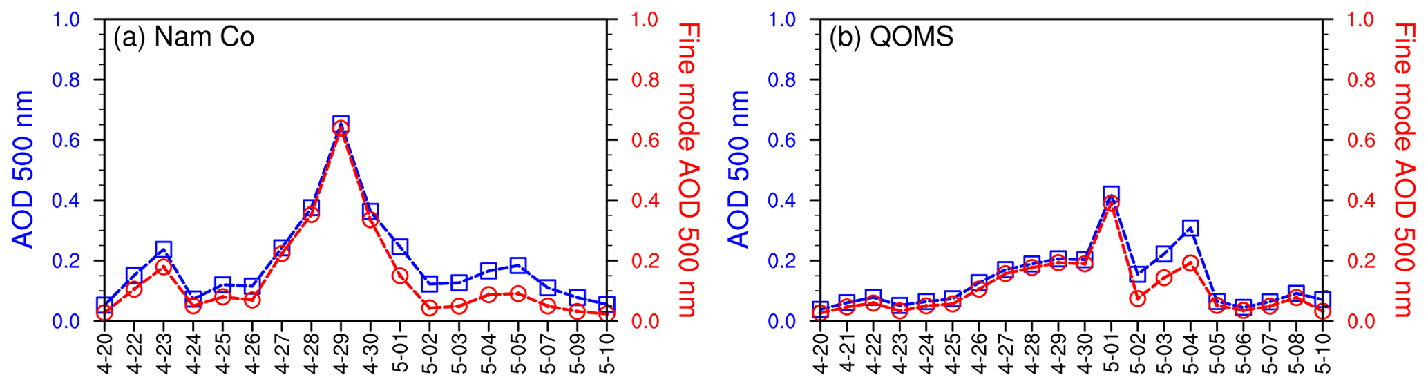
Figure 1 Time series of daily mean AOD (blue) and fine-mode AOD (red) at 500 nm at Nam Co (a) and QOMS (b) stations during the period from 20 April to 10 May 2016.

2.3 WRF-Chem model configuration, emissions, and experimental design

The WRF-Chem model is a fully coupled regional dynamical and chemical transport model that considers the gas-phase chemistry, photolysis, and aerosol mechanism (Grell et al., 2005). The model can simulate the emission, transport, mixing, chemical reactions, and deposition of trace gases and aerosol simultaneously with the meteorological fields. It has been successfully applied in air pollution studies over the TP and adjacent regions (Yang et al., 2018; Chen et al., 2018; Hu et al., 2022b). The version used in this study is based on v3.9.1. As shown in Fig. 2, the simulation domain is centered at 31^∘ N, 87.5^∘ E and covers the whole TP and its surroundings. Numerous previous modeling studies on aerosol–meteorology feedback were carried out using a model domain with a horizontal resolution of 20 km or even coarser (Hu et al., 2022a; Zhang et al., 2018a; Li et al., 2022; Bharali et al., 2019; Gao et al., 2015; Huang et al., 2020). Considering that the topography over the TP is very complex, model simulations in this study are conducted at a 15 km horizontal resolution using Lambert conformal mapping with 259 (west–east) × 179 (north–south) grid cells. For all grids, there are 30 vertical sigma levels extending from the surface to 50 hPa. The key physical parameterization options used in this study include the Noah land surface model (Ek et al., 2003; Chen et al., 2010) and the Monin–Obukhov scheme for the surface layer physical processes (Srivastava and Sharan, 2017), the double-moment Morrison microphysical parameterization (Morrison et al., 2009) with the Grell–Freitas (GF) cumulus scheme (Grell and Freitas, 2014), the Mellor–Yamada–Janjic (MYJ) planetary boundary layer scheme with local vertical mixing (Janjiæ, 1994), and the Rapid Radiative Transfer Model for General circulation models (RRTMG) coupled with the aerosol radiative effect for both longwave and shortwave radiation (Iacono et al., 2008). With respect to the chemical parameterization options, the Carbon-Bond Mechanism version Z (CBMZ) gas-phase chemistry mechanism (Zaveri and Peters, 1999) combined with the Model for Simulating Aerosol Interactions and Chemistry (MOSAIC) aerosol module (Zaveri et al., 2008) was chosen for aerosol simulation. The MOSAIC aerosol scheme uses a segmentation approach to represent the aerosol size distribution with four or eight discrete size bins (Fast et al., 2006). In this paper, the aerosol size is divided into four bins. Aerosol species simulated by the MOSAIC scheme include sulfate, methanesulfonate, nitrate, chloride, carbonate, ammonium, sodium, calcium, BC, primary organic mass, liquid water, and other inorganic mass.

The initial and boundary conditions for meteorological fields are obtained from the National Centers for Environmental Prediction (NCEP) Final Analysis (FNL) data with a ${\mathrm{1}}^{\circ }\times {\mathrm{1}}^{\circ }$ spatial resolution and a 6 h temporal resolution (https://rda.ucar.edu/datasets/ds083.2/, last access: 23 August 2022). Anthropogenic emissions, such as CO, VOCs, NO_x, NH₃, BC, OC, SO₂, PM_2.5, and PM₁₀, are taken from the Emission Database for Global Atmospheric Research (EDGAR)-Hemispheric Transport Air Pollution version 2 (HTAPv2) emission inventory (https://edgar.jrc.ec.europa.eu/dataset_htap_v2, last access: 19 August 2022) for the year 2010. Detailed information on the HTAP inventory can be found in Janssens-Maenhout et al. (2015). The biogenic emissions are based on the Model of Emissions of Gases and Aerosols from Nature (MEGAN) (Guenther et al., 2006; Guenther et al., 2012), and the biomass burning emissions were calculated with high-resolution fire emissions based on the Fire INventory from NCAR (FINN) (Wiedinmyer et al., 2011). In addition, the mozbc utility and the Community Atmosphere Model with Chemistry (CAM-Chem) (Buchholz et al., 2019) dataset are used to create improved chemical initial and boundary conditions. The simulation is conducted from 10 April to 10 May 2016, and the first 10 days are used for model spin-up. The results from 20 April to 10 May 2016 are used for the analysis.

There are two experiments in this study: one is the control experiment (CONT) and the other is the sensitive experiment (SEN). In the CONT, the simulation is conducted using the WRF-Chem model with aerosol–meteorology feedback turned on. The SEN is exactly the same as the CONT except that the feedback between aerosol and meteorology is turned off. The difference between the CONT and the SEN is considered as the effect induced by aerosol–meteorology feedback.

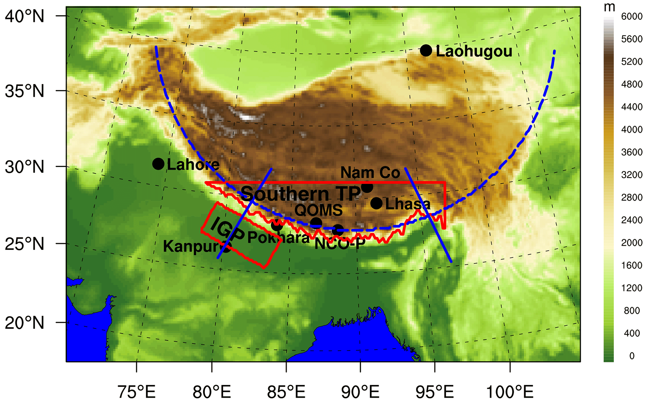
Figure 2 WRF-Chem model domain and terrain (shading; m). Solid black dots denote stations used to verify the model performance for meteorological conditions and aerosols. The regions demarcated by solid red lines denote the southern TP and the Indo-Gangetic Plain. The dashed blue line and two solid lines represent the cross sections used for analysis in this paper.

3 Results and discussion

3.1 Meteorological causes of the severe aerosol pollution event

Excessive emissions and adverse meteorological conditions are the two most important factors influencing air quality (Wang et al., 2019; Y. Chen et al., 2019; Liu et al., 2017; Zhang et al., 2019). The TP, which has a small population density and a low degree of industrialization, is one of the most pristine regions on the earth. Moreover, as mentioned above, from 27 April to 4 May 2016, the AOD at the background stations of Nam Co and QOMS, with few human activities, is significantly higher than that of the baseline, with the highest value being at least one order of magnitude than that of baseline. Therefore, it can be inferred that aerosols over the TP during this severe aerosol pollution event are mainly sourced from adjacent regions by long-range transport, which is consistent with the results reported in a previous study (Kang et al., 2019b). Atmospheric circulation, the main driving force of atmospheric aerosols, plays a substantial role in the long-range transport of aerosols. Therefore, with little change in the emission source, analyzing the meteorological conditions during a severe pollution event is crucial. Figure 3 shows weather maps at 500 hPa based on the ERA-Interim reanalysis dataset. It is found that, during 08:00–14:00 Beijing Time (hereafter “BJT”) on 27 April, straight westerly airflow prevailed at 500 hPa over the TP (Fig. 3a), which transported aerosols from northwestern South Asia to the TP. Subsequently, wind field shear occurred over the plateau at 20:00 on 27 April (Fig. 3b), and a plateau vortex was generated at 02:00 on 28 April (Fig. 3c), which was conducive to the accumulation of aerosols in the inland of the plateau. From 08:00 on 28 April to 08:00 on 29 April, the plateau vortex stabilized over the TP and the aerosol concentrations at Nam Co station continued to increase (figure not shown). At 14:00 on 29 April, the plateau vortex disappeared (Fig. 3d) and the aerosol concentrations peaked at Nam Co station. Meanwhile, a high-pressure system was located on the west side of the plateau, accompanied by a trough on the foreside (Fig. 3d). Thus, southwesterly airflow in front of the trough transported aerosols from northern South Asia to the southern TP (Fig. 3e). As a result, the aerosol concentrations at QOMS station increased and peaked on 1 May. At 14:00 on 1 May, the high-pressure system moved eastward from the west side to the inland of the TP, and northerly winds ahead of this high-pressure system prevailed over the TP (Fig. 3f) and wafted aerosols away from the TP, so aerosol concentrations at QOMS station began to decrease.

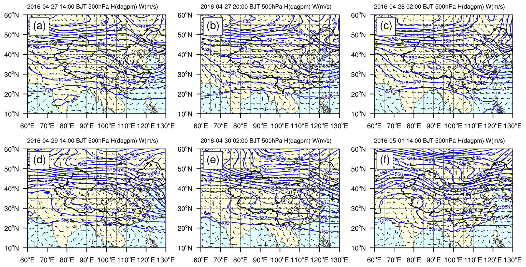
Figure 3 Weather maps at 500 hPa over the study area during the severe aerosol pollution event, based on the ERA-Interim reanalysis dataset. The blue lines are isopleths of geopotential height (unit: dagpm). Wind speed (unit: m s⁻¹) and direction are denoted by wind barbs.

3.2 Evaluating model performance for meteorology and chemistry

3.2.1 Validation of model performance for meteorology

Validating the model performance for meteorology is critical for assuring accuracy when simulating aerosol concentrations. This is because the meteorological conditions are closely associated with aerosol growth, transport, and deposition. Herein, to validate the model performance for meteorological conditions, the temporal variation in the simulated and reanalyzed T₂, RH2, and U₁₀ at Nam Co, QOMS, Kanpur, and Lahore stations is shown in Fig. S2. The model represents the correct temporal trends in T₂ at the four stations reasonably well, although underestimations are detected at Nam Co and QOMS stations. The variation trend in RH2 from the simulation is highly consistent with that obtained from reanalysis at Kanpur and Lahore stations. However, at Nam Co and QOMS stations, a larger discrepancy is observed between simulation and reanalysis, which might be related to the high altitude and complex topography there. For U₁₀, the simulated trends coincide on average with the observed trends at Nam Co, Kanpur, and Lahore stations. The corresponding statistics, including sample size (N), observed mean, simulated mean, mean bias (MB), normalized mean bias (NMB), root mean square error (RMSE), and correlation coefficient (R) between the observations and the simulation at different stations, are shown in Table S1 in the Supplement. The calculations indicate that T₂ is well simulated, with MBs of −4.25, −3.62, 0.03, and 0.07 and R values of 0.69, 0.87, 0.94, and 0.96 at Nam Co, QOMS, Kanpur, and Lahore stations, respectively. RH2 and U₁₀ are less well simulated, especially at Nam Co and QOMS stations, where the altitude is very high and the terrain is fairly complex. To be exact, MBs of 29.68 and −25.82 and R of 0.51 and 0.52 are obtained for RH2 at Nam Co and QOMS stations, respectively, and MBs of 0.91 and 5.66 and R values of 0.30 and 0.55 are detected for U₁₀ at the two stations. However, at Kanpur and Lahore stations, both the RH2 and U₁₀ from reanalysis and simulation are highly consistent, with MBs of −12.56 and 0.85, −13.00 and 0.96, and Rs values of 0.80 and 0.45, 0.78 and 0.22, respectively. On the whole, U₁₀ is overestimated on average at four stations and has a greater range of about 3.43–8.56 m s⁻¹ compared to the reanalyzed values, which have a range of about 2.47–3.39 m s⁻¹. Hence, the simulations are biased, at least in part, since the model grid represents the regional average for 15×15 km² in a domain of great topographic complexity, and the values derived from reanalysis with a horizontal resolution of ${\mathrm{0.05}}^{\circ }\times {\mathrm{0.05}}^{\circ }$ represent regional averages obtained at higher resolution. In addition, the accuracy of the gridded observational data of ERA-Interim is correlated with the restriction on the observations assimilated into the reanalysis and with the different assimilation methods (Chung et al., 2013). Overall, we can conclude that the WRF-Chem model exhibits acceptable performance in simulating temporal variations in meteorological elements.

The spatial distributions of T₂, RH2, and the wind field at 500 hPa from simulation and reanalysis over the domain are presented in Fig. S3. Spatially, both simulation and reanalysis show similar spatial patterns for each of the abovementioned meteorological fields. To be exact, high surface air temperatures mainly appear over regions surrounding the TP; this is especially obvious over South Asia, where the surface air temperature exceeds 30 ^∘C. Previous studies indicated that the surface air temperature over the Indian subcontinent is highest during the pre-monsoon season because the Himalayas block the frigid katabatic winds that flow down from Central Asia during this period (Ji et al., 2011). In contrast, low surface air temperatures mainly occur over the TP. Different from T₂, high RH2 values primarily appear over the TP, the Bay of Bengal, and central and eastern China, but low values occur in the rest of the domain. In particular, RH2 is apparently higher in the southeastern TP than in the inland of the TP because the southeastern TP is in proximity to moisture sourced from the Bay of Bengal. Moreover, the reason why the spatial distribution of T₂ is in antiphase with that of RH2 is that the decrease in T₂ can lead to a decrease in the saturation pressure of water vapor and an increase in RH2 at the surface (Gao et al., 2015). With respect to the 500 hPa wind field, both the simulation and observations show that westerly winds prevail over the entire region. Due to the high topography of the TP, these westerly winds are divided into two branches at appropriate 75^∘ E. One branch flows eastward and the other branch is forced up by the high plateau and subsequently shifts to become a northwesterly wind. Therefore, the WRF-Chem model also effectively simulates the spatial distributions of T₂, RH2, and the 500 hPa wind fields. Overall, this simulation configuration captures the meteorological fields well, which is critical to assuring the simulation accuracy for air pollutant concentrations.

3.2.2 Validation of model performance for AOD and BC

To validate the model performance in simulating spatiotemporal variations in aerosols, ground-based AOD data from AERONET together with reanalyzed AOD data from MERRA-2 are first compared to the simulated AOD. Figure S4 shows the temporal variations in simulated and observed daily mean AOD at Nam Co, QOMS, and Pokhara stations for the period from 20 April to 10 May 2016. As a whole, the WRF-Chem model reasonably reproduces the temporal variations in AOD at each of the above stations, with a larger bias occurring at Nam Co and Pokhara stations and a smaller bias at QOMS station. The specific statistics for N, the observed mean, the simulated mean, MB, NMB, RMSE, and R between the observed and simulated AODs at different stations are shown in Table S2. As one-third of the AOD values at the selected stations in the MERRA-2 dataset during the study period are missing, the statistical description of the reanalyzed and simulated AOD is not presented. The results from Table S2 indicate that MB values of −0.13, −0.01, and −0.57 and R values of 0.58, 0.42, and 0.56 are obtained at Nam Co, QOMS, and Pokhara, respectively. Moreover, the AOD from observations is significantly correlated with that from the simulation at Nam Co and Pokhara stations, with the correlation coefficient passing the 95 % confidence level. In addition, we note that the AOD from the simulation is on average lower than that from observations, which may be due to the assumption of spherical aerosol particles in the model simulation. The optical properties of particles are more sensitive to a nonspherical morphology than a primarily spherical structure (China et al., 2015; He et al., 2015). On the whole, the model effectively reproduces the observed temporal variation in AOD.

The spatial pattern of simulated AOD is consistent with that from either the MODIS or MERRA-2 reanalysis dataset, suggesting that WRF-Chem performs reliably when simulating AOD. Specifically, the AODs from simulation, MODIS, and MERRA-2 show distinct spatial distribution characteristics, with high values in northern South Asia, the Bay of Bengal, Southeast Asia, and the Sichuan Basin and low values over the TP (Fig. S5). This is because northern South Asia, Southeast Asia, and the Sichuan Basin are heavily industrialized and densely populated regions compared to the TP (Bran and Srivastava, 2017). In the Taklimakan Desert, the AOD monitored by satellite is much higher than that obtained from simulation, which is likely due to the uncertainty of the emission inventory. Taken together, the comparison between the simulation from WRF-Chem and observations from AERONET, MODIS, and MERRA-2 shows that the WRF-Chem model captures the overall spatiotemporal characteristics of AOD over the domain.

To verify the capability of this framework for WRF-Chem when simulating the BC concentration, we present the temporal variation in simulated and reanalyzed hourly BC concentrations at Nam Co, QOMS, Lhasa, NCO-P, Laohugou, and Kanpur stations during the period from 20 April to 10 May 2016, as shown in Fig. 4. It is found that, overall, the WRF-Chem model reproduces the temporal variation in reanalyzed BC concentrations at different stations. The specific statistics for N, the observed mean, the simulated mean, MB, NMB, RMSE, and R when comparing the reanalyzed and simulated hourly BC concentrations at different stations are shown in Table S2. As can be seen, MB values of −0.07, 0.14, −0.02, −0.02, 0.02, and 0.72 and R values of 0.67, 0.43, 0.47, 0.50, 0.25, and 0.64 are obtained at Nam Co, QOMS, Lhasa, NCO-P, Laohugou, and Kanpur stations, respectively. The reanalyzed and simulated hourly BC concentrations are strongly correlated at each of the stations, with the correlation coefficient exceeding the 99 % confidence level. Besides the reanalyzed hourly BC concentrations, in situ observations of BC are available for the QOMS station. An intercomparison between the in situ observed, simulated, and MERRA-2 reanalyzed daily mean BC concentrations at the QOMS station was also conducted, as shown in Fig. S6. It is apparent that the temporal variation in simulated daily mean BC concentrations is very close to that of the observed daily mean BC concentrations. The correlation coefficient between the simulated and observed daily mean BC concentrations is 0.867, which exceeds the 99 % confidence level. Hence, the WRF-Chem model exhibits better performance in simulating BC concentrations.

Because the spatial distribution of BC concentrations retrieved from the CAM_Chem dataset is not reasonable (Fig. S7a), an intercomparison between the WRF-Chem simulated and the reanalyzed BC concentrations over the domain was performed to validate the model performance for the spatial distribution of BC concentrations. Figure S7b–c presents the spatial distribution of simulated and reanalyzed BC concentrations over the domain averaged for the period from 20 April to 10 May 2016. It is found that BC concentrations from both the simulation and reanalysis display distinct spatial variability, with low concentrations over the TP and high concentrations over the north of South Asia, Southeast Asia, and the Sichuan Basin. As it is one of the most pristine regions on the earth, the TP has a small population density and a low degree of industrialization, resulting in low BC concentrations. Nonetheless, regions adjacent to the TP with low elevations, like northern South Asia, Southeast Asia, and the Sichuan Basin, have dense populations and high industrialization (Li et al., 2016a, b; Qin and Xie, 2012), so they emit large amounts of BC into the atmosphere, resulting in high BC concentrations. Therefore, the WRF-Chem model can capture the main temporal and spatial features of BC concentrations over the TP and adjacent regions.

Figure 4 Temporal variations in simulated and reanalyzed hourly BC concentrations at Nam Co (a), QOMS (b), Lhasa (c), NCO-P (d), Laohugou (e), and Kanpur  (f) stations for the period from 20 April to 10 May 2016.

3.3 Transboundary transport flux of BC

The foregoing analysis validated the model framework used in this study and found that the results obtained from it are basically satisfactory. As BC is the major component of light-absorbing particles, it exerts a significant impact on climatic and cryospheric changes over the TP due to its strong light absorption and important effect on the albedo of snow and ice (Kang et al., 2010, 2019b; Yang et al., 2018). In this section, the transboundary transport flux of BC during this severe aerosol pollution event is investigated. According to a previous study, the BC transport flux can be calculated by projecting the wind field perpendicularly to the cross line, which is then multiplied by the BC mass concentration (Zhang et al., 2020). More specifically, the BC transport flux is calculated as follows:

$$\begin{array}{}\text{(1)}& \mathrm{TF}=\mathrm{C}\cdot \left(u\cdot \sin \mathit{\alpha }+v\cdot \sin \mathit{\beta }\right),\end{array}$$

where α is the angle between the east–west wind component and the cross line, β is the angle between the south–north wind component and the cross line, and C is the BC mass concentration at the grid along the cross line. Here u and v are the wind components. The flux is estimated at each model level. Positive values represent transport towards the TP, while negative values represent transport away from the TP. Figure 5 presents longitude–height cross sections of BC transport flux along the cross line (shown as the dashed blue lines in Fig. 2) at 15:00 and 03:00 BJT (to represent daytime and nighttime transport, respectively) averaged for the period from 27 April to 4 May (the most polluted period) obtained from the simulation with aerosol–meteorology feedback. Notably, in the central and western Himalayas (to the west of ∼94 ^∘E), BC is imported into the TP during both daytime and nighttime (this is especially obvious at heights below 7 km), although the transport flux during the nighttime is higher than that during the daytime. In the eastern Himalayas (from 94–98^∘ E), BC is imported into the TP during the day but exported slightly from the TP during the night. To the east of ∼98^∘ E, BC is transported away from the TP during the day and night due to the prevailing westerly winds. Generally, the transport across the western Himalayas is controlled by the large-scale westerly, while the transport across the central and eastern Himalayas is primarily dominated by a local southerly (Zhang et al., 2020). Therefore, the difference in BC transport flux between the western and eastern Himalayas is attributed to the influence of a large-scale westerly that is weak over the eastern Himalayas. The stronger diurnal variation of the local southerly (which is directed toward the TP in the daytime and away from the TP in the nighttime) compared to that of the westerly near the surface leads to the large difference in the diurnal variation of the transport between the western and eastern Himalayas. In addition, the largest BC transport flux along the cross line occurs at deeper mountain valley channels (Fig. 5). Zhang et al. (2020) investigated the impact of topography on BC transport to the southern TP during the pre-monsoon season and found that the BC transport across the Himalayas is able to overcome the majority of mountain ridges but that valley transport is more efficient, which is consistent with the results obtained in this study.

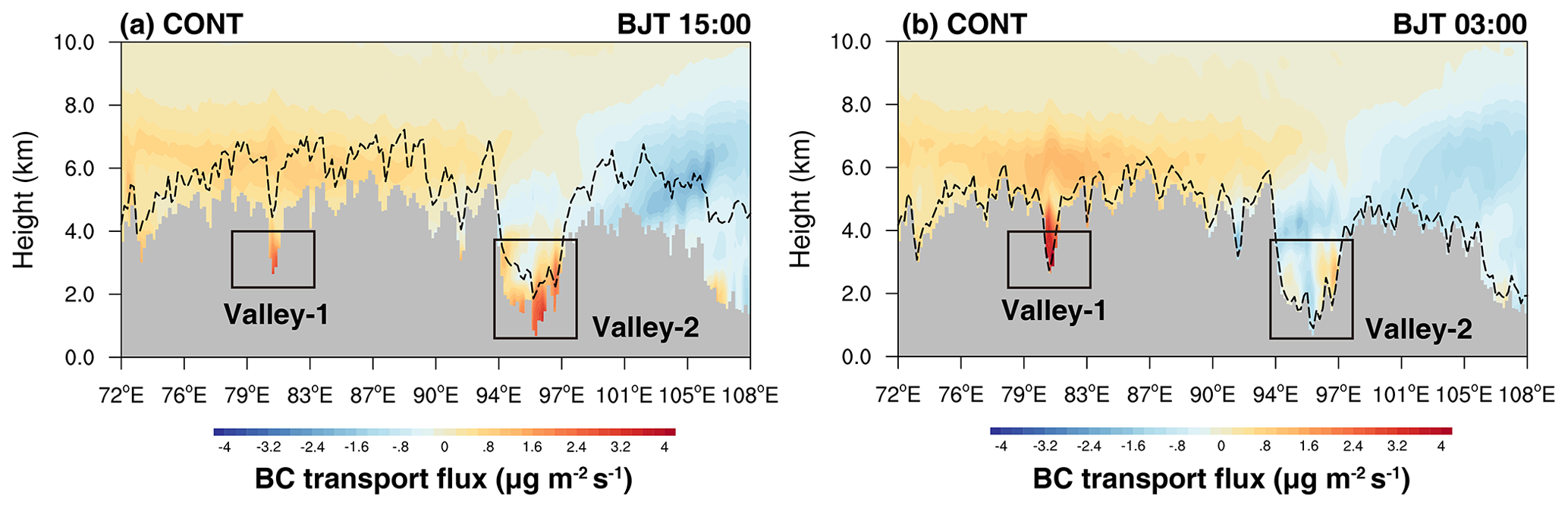
Figure 5 Longitude–height cross sections of BC transport flux along the cross line (shown as the dashed blue line in Fig. 2) at 15:00 and 03:00 BJT averaged for the period from 27 April to 4 May 2016 obtained from simulation with aerosol–meteorology feedback. The planetary boundary layer height (PBLH) along the cross section is shown here as a dashed black line.

As the largest BC transport flux occurs at deeper mountain valleys, the two deepest mountain valley channels along the cross line shown as a solid blue line in Fig. 2 are selected to demonstrate the BC transport flux across mountain valleys during this severe pollution event. The first valley (referred to as “valley-1” hereon) is located in the southwestern TP, while the second valley (referred to as “valley-2” hereon) is located in the southeastern TP. It is seen that, at valley-1, the overall positive values near the surface indicate that BC is imported into the TP during the daytime and nighttime, though the transport flux at night is much higher than that during the daytime (Fig. 5). The averaged BC concentration and transport flux at 03:00 and 15:00 BJT during the period from 27 April to 4 May 2016 across valley-1 from the simulation with aerosol–meteorology feedback also shows that the BC transport flux is much higher during the night than during the daytime (Fig. 6a, b). By checking the surface BC concentration from simulation with aerosol–meteorology feedback, it is found that the surface BC concentration at valley-1 during the night is much higher than that during the daytime (Table 1). Moreover, the vertically integrated BC concentration over the Himalayas is much higher in the nighttime than in the daytime (Fig. S8). With the help of the large westerly winds, BC is then transported to the TP, which provides further evidence for the higher BC transport flux during the night shown in Fig. 6b. At valley-2, the positive near-surface flux values during the daytime and the negative values during the night denote that BC is imported into the TP during the daytime but exported slightly from the TP at night (Fig. 5). To analyze this distinct diurnal variation in BC transport flux, we present the latitude–height cross sections of the BC transport flux and its concentration at 03:00 and 15:00 BJT averaged for the period from 27 April to 4 May 2016 across valley-2 obtained from the simulation with aerosol–meteorology feedback, as shown in Fig. 6c, d. Notably, the deeper planetary boundary layer height (PBLH) and the strong turbulent mixing during the daytime over northern India cause BC to be mixed at a higher altitude (Fig. 6c). Subsequently, the local southerlies boost BC transport across the eastern Himalayas towards the TP. Nevertheless, during the night, the meridional wind is dominated by a northerly over the eastern Himalayan region (Fig. 6d), suggesting that cross-Himalayan transport is directed away from the TP.

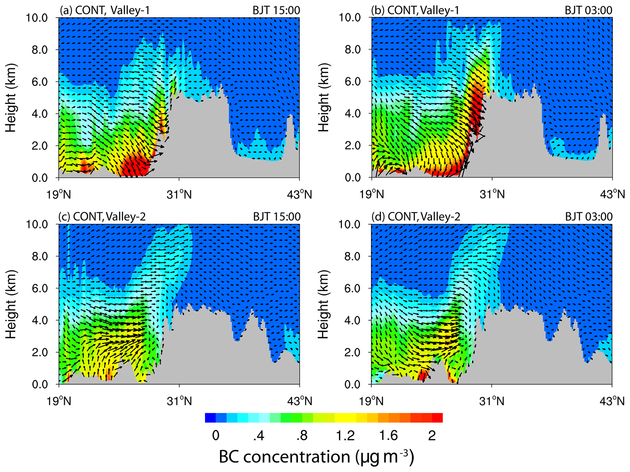
Figure 6 Latitude–height cross sections of BC transport flux (vector) across (a, b) valley-1 and (c, d) valley-2 at 15:00 and 03:00 BJT averaged for the period from 27 April to 4 May 2016 from simulation with aerosol–meteorology feedback. The contours represent the BC concentrations.

Table 1 Surface BC concentrations at two typical mountain valley channels at 15:00 and 03:00 BJT averaged for the period from 27 April to 4 May 2016 from simulation with aerosol–meteorology feedback.

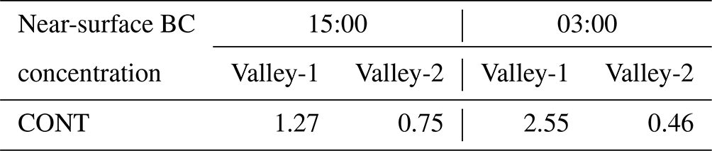
To further demonstrate the overall inflow flux across the Himalayas, the vertically integrated BC mass flux along the longitudinal cross section shown in Fig. 5 from simulation with aerosol–meteorology feedback is shown in Fig. 7. The total mass flux is calculated by integrating the right-hand term of Eq. (1) as follows:

$$\begin{array}{}\text{(2)}& \text{ITF}=\underset{z=z_{\text{sfc}}}{\overset{z=z_{\text{top}}}{\int }}\mathit{\delta }z\cdot C\cdot \left(\mathit{\mu }\cdot \sin \mathit{\alpha }+v\cdot \sin \mathit{\beta }\right),\end{array}$$

where δz is the thickness of each vertical model level. Similarly, positive flux values represent transport towards the TP, while negative values represent transport away from the TP. It is found that there are primarily positive values in the central and western Himalayas (to the west of 92^∘ E) and primarily negative values to the east of 92^∘ E (Fig. 7). Furthermore, the vertically integrated transport flux of BC along the cross line is strongly correlated with the longitudinal degree of the cross line: the correlation coefficient reaches up to −0.89, passing the 99 % confidence level. This indicates that the vertically integrated transport flux of BC along the cross line decreases from west to east. In particular, from 80 to 86^∘ E along the cross line, the correlation coefficient between the terrain height and the vertically integrated transport flux of BC is −0.87, exceeding the 99 % confidence level, suggesting that the lower the valleys, the higher the vertically integrated transport flux across the Himalayas can be. In particular, the largest vertically integrated transport flux, about 20.8 mg m⁻² s⁻¹, occurs at valley-1. However, in the eastern Himalayas (to the east of ∼92^∘ E), the BC is exported from the TP overall, and the vertically integrated transport flux with the largest value (near to zero) occurs at valley-2.

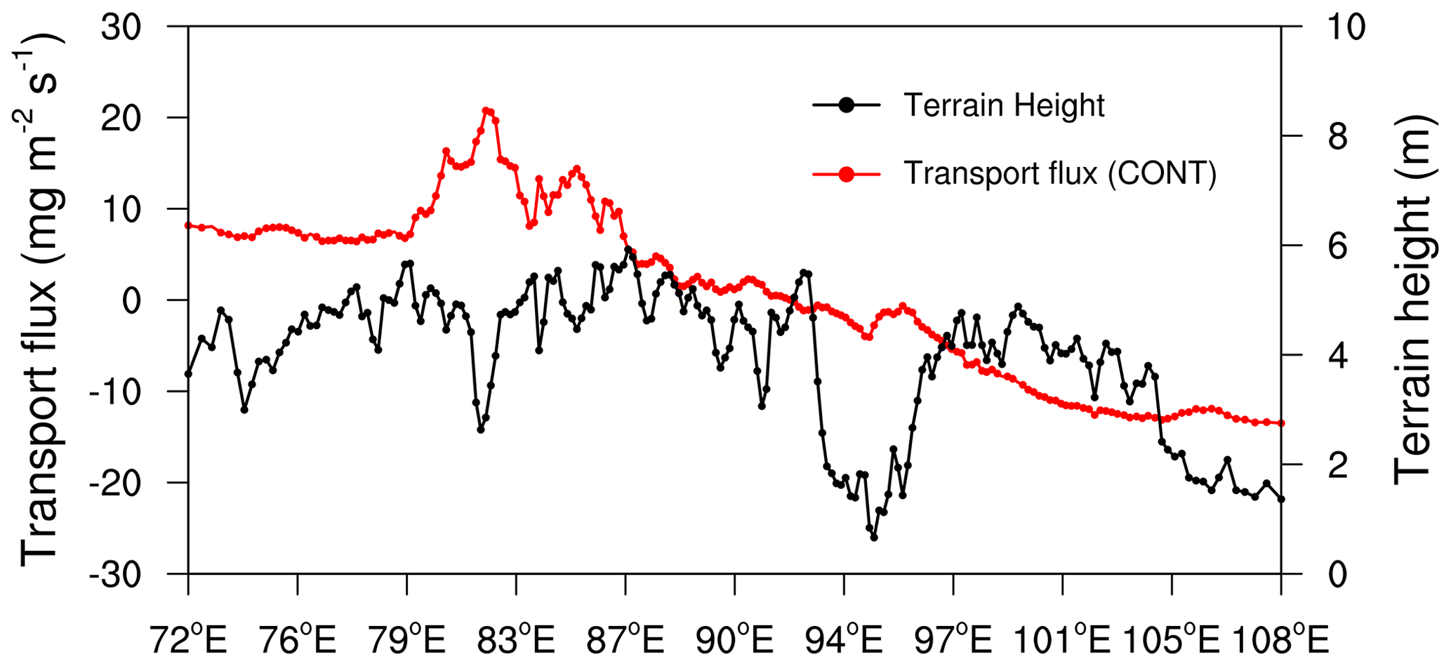
Figure 7 Longitudinal distribution of the vertically integrated BC mass flux (red line) along the cross section shown in Fig. 2 from simulation with aerosol–meteorology feedback. The black line represents the terrain height.

3.4 Aerosol–meteorology feedback during the severe aerosol pollution event

Generally, a severe aerosol pollution event is accompanied by complex feedback between aerosol and meteorology. The analysis above confirms that BC in northern South Asia could have been transported to the TP via the cross-Himalayan transport during this severe pollution event. Moreover, compared to the eastern Himalayas, the western Himalayas contribute more BC to the TP, and BC from the cross-Himalayan transport is mainly concentrated in the southern TP. Therefore, in this section, the feedback between aerosol and meteorology over the western Indo-Gangetic Plain (referred to as “IGP” hereon) and the southern TP during this severe pollution event is analyzed.

To illustrate the aerosol radiative forcing (ARF) and its impacts on T₂, RH2, surface energy, atmospheric stability, wind, and the PBLH over the southern TP and IGP regions, time series of aerosol-induced daily and diurnal changes in meteorological variables (T₂, RH2) and the surface energy budget (latent heat (LH), sensible heat (SH), shortwave (SW) radiation, longwave (LW) radiation, and net energy flux (LH + LW + SH + SW)) averaged for the southern TP and IGP regions are shown in Fig. 8. These time series were calculated by subtracting the model results of SEN from those of CONT. It should be noted that the diurnal change was calculated for the most polluted period from 27 April to 4 May. As can be seen, the daily variation in aerosol-induced area-averaged surface air temperature ranged from −0.1 to 0.1 ^∘C in the southern TP, with discernible decreases of 0.1 ^∘C appearing on 2, 4, 6–7 May (Fig. 8a), and ranged from −1.7 to 1.2 ^∘C in the IGP (Fig. 8c) during the period from 20 April to 1 May. During the most polluted period from 27 April to 4 May, the aerosol-induced surface air temperature ranged from −0.1 to 0.1 ^∘C in the southern TP (Fig. 8a), with decreases of 0.1 ^∘C observed on 2 and 4 May, and decreased by 0.5–1.7 ^∘C in the IGP (Fig. 8c). The daily variation in aerosol-induced area-averaged RH2 displayed a slight change over the southern TP (Fig. 8a), with values ranging from −1.6 % to 2.3 %, and exhibited a greater range of about −10.9 % to 13.7 % in the IGP (Fig. 8c) during the period from 20 April to 1 May. From 27 April to 4 May (the period with high aerosol concentrations), the area-averaged RH2 increased by 0 %–2.3 % and by 0.8 %–13.7 % in the southern TP and IGP, respectively (Fig. 8a, c). For the diurnal change depicted in Fig. 8b and d, during 09:00–20:00 BJT in the daytime, the aerosol-induced area-averaged surface air temperature had a range of about −0.1 to 0.1 ^∘C in the southern TP and decreased by 0.9–2.3 ^∘C in the IGP. At night, the surface air temperature increased by 0.1 ^∘C during 00:00–05:00 BJT in the southern TP (Fig. 8b) and decreased by 0–1.0 ^∘C during 21:00–08:00 BJT in the IGP (Fig. 8d). The corresponding diurnal change in aerosol-induced RH2 indicated that the aerosol-induced RH2 decreased by 0.1 %–0.4 % during 14:00–17:00 BJT in the southern TP but increased during the rest of the day, with the maximum increase of 1.3 % occurring during 09:00–10:00 BJT (Fig. 8b). In the IGP, the aerosol-induced RH2 increased by 3.3 %–7.1 % during 09:00–20:00 BJT in the daytime and increased by 2.6 %–4.5 % during 21:00–08:00 in the nighttime (Fig. 8d). Therefore, the aerosol-induced changes in T₂ and RH2 primarily occur in the daytime.

Generally, positive surface energy values indicate more energy flux toward the surface and vice versa. Figure 8e–h shows the aerosol-induced surface energy changes over the southern TP and IGP. It is found that the SW radiation flux at the surface decreased by 0–13.7 W m⁻² in the southern TP (Fig. 8e) and by 44.5–75.3 W m⁻² in the IGP (Fig. 8g) during the period from 27 April to 4 May due to the absorption and scattering of solar radiation by aerosol. In contrast, LW radiation flux at the surfaces of the southern TP and IGP increased due to the positive radiative forcing of aerosol in the atmosphere, with an increase of 4.1–4.6 W m⁻² observed in the southern TP from 30 April to 1 May (Fig. 8e) and a large increase of 12.3–23.4 W m⁻² observed in the IGP from 27 April to 4 May (Fig. 8g). Because of the aerosol's radiative cooling effects, the LH and SH fluxes from the surface to the atmosphere in both regions decreased. In particular, in the southern TP, the maximum decreases in the LH and SH fluxes, 2.0 and 7.8 W m⁻², respectively, occurred on 30 and 29 April, respectively (Fig. 8e). In the IGP, the LH and SH fluxes decreased by 4.1–7.4 W m⁻² and by 26.6–43.6 W m⁻², respectively, from 27 April to 4 May (Fig. 8g). The net energy flux at the surface decreased by 1.6–18.8 W m⁻² in the southern TP (Fig. 8e) and by 62.7–104.3 W m⁻² in the IGP (Fig. 8g) from 27 April to 4 May. Therefore, the energy arriving at the surfaces of the southern TP and IGP decreased during this severe aerosol pollution event. For the diurnal change in surface energy, during 09:00–20:00 BJT in the southern TP, the SW, LH, SH, and net energy fluxes decreased by 7.8–19.9, 0–2.4, 4.7–12.2, and 13.4–29 W m⁻², respectively, while the LW flux increased by 0.3–2. W m⁻² (Fig. 8f). During 09:00–20:00 BJT in the IGP, the SW, LH, SH, and net energy fluxes decreased by 46.1–144.2, 7.5–16.6, 9.6–100.1, and 54.7–221.5 W m⁻², respectively, whereas the LW flux increased by 8.5–30.5 W m⁻² (Fig. 8h). Therefore, changes in surface energy mainly occur during the daytime.

Figure 8 Time series of aerosol-induced daily changes in (a, c) meteorological variables (T₂ (^∘C), RH2 (%)) and (e, g) the surface energy budget (SH, LH, LW radiation, SW radiation, and net energy flux, Wm⁻²) averaged for the (a, e) southern TP and (c, g) IGP during the period from 20 April to 1 May. Time series of aerosol-induced diurnal changes in (b, d) meteorological variables and (f, h) the surface energy budget averaged for the period from 27 April to 4 May 2016 for the (b, f) southern TP and (d, h) IGP. LH is latent heat, LW is longwave radiation, SH is sensible heat, SW is shortwave radiation, and NET is the sum of the total energy fluxes.

Figure 9 shows the spatial distributions of aerosol-induced changes in T₂ and RH2 and aerosol radiative forcing (ARF) at the bottom of the atmosphere as well as in the atmosphere, calculated by subtracting the model results of SEN from those of CONT averaged during 09:00–20:00 BJT from 27 April to 4 May. As seen in Fig. 9a, the aerosol-induced surface air temperature decreased over most parts of the study area except for the TP, where the surface air temperature increased; this was especially obvious in the northern TP, where the surface air temperature increased by up to 1.0 ^∘C. Because the TP is one of the most pristine regions on the earth and has few human activities, there is significantly less aerosols over the TP compared to the regions surrounding the TP. Consequently, the surface-reaching solar radiation over the TP in the daytime is higher than that over its surroundings, leading to higher surface temperatures. A decrease in the surface-reaching solar radiation during daytime can lead to a decline in the surface air temperature. From Fig. 9a, the largest surface air temperature decrease due to aerosols occurred in South Asia, since South Asia has large amounts of aerosols due to rapid economic growth, industrialization, and unplanned urbanization compared to other regions (Shi et al., 2020). The spatial distribution of aerosol-induced changes in RH2 is opposite to that of T₂, with increased RH2 appearing in most parts of the study area and decreased RH2 on the TP. Specifically, the largest increase in RH2 occurred in northern South Asia, since the aerosol-induced change in the water vapor mixing ratio is very small, and the decrease in temperature can lead to a decrease in the saturation pressure of water vapor and an increase in RH2 at the surface, which is beneficial for the hygroscopic growth of aerosols (Gao et al., 2015). By analyzing the time–altitude distribution of the diurnal cycle of aerosol impacts on temperature and relative humidity (RH) averaged for the southern TP and IGP during the period from 27 April to 4 May , it is found that, consistent with the aerosol-induced changes in T₂ and RH2, the aerosol-induced changes in temperature and RH mainly occurred during daytime as well (Fig. S9). Specifically, in the southern TP, the maximum increase in temperature, up to 0.15 ^∘C, occurred in the middle troposphere (Fig. S9a). However, in the IGP, the temperature decreased near the surface, with a maximum drop of more than 0.3 ^∘C, and it increased in the middle troposphere, with a maximum increase of more than 0.3 ^∘C (Fig. S9c). There is no doubt that such a temperature change increases the stability of the atmosphere over both regions. Note that the temperature increase in the middle troposphere over the southern TP is more significant than that in the IGP, which is possibly correlated with the thermal pump role of the TP (Li and Yanai, 1996; Meehl, 1994; Yanai et al., 1992). The time–altitude distribution of the diurnal cycle of RH is opposite to that of temperature, with RH increasing near the surface and decreasing in the middle troposphere (Fig. S9b and d). To be exact, RH decreased by 1.6 % in the middle troposphere over the southern TP (Fig. S9b); in the IGP, RH increased near the surface by more than 3 % and decreased by more than 3 % in the middle troposphere (Fig. S9d).

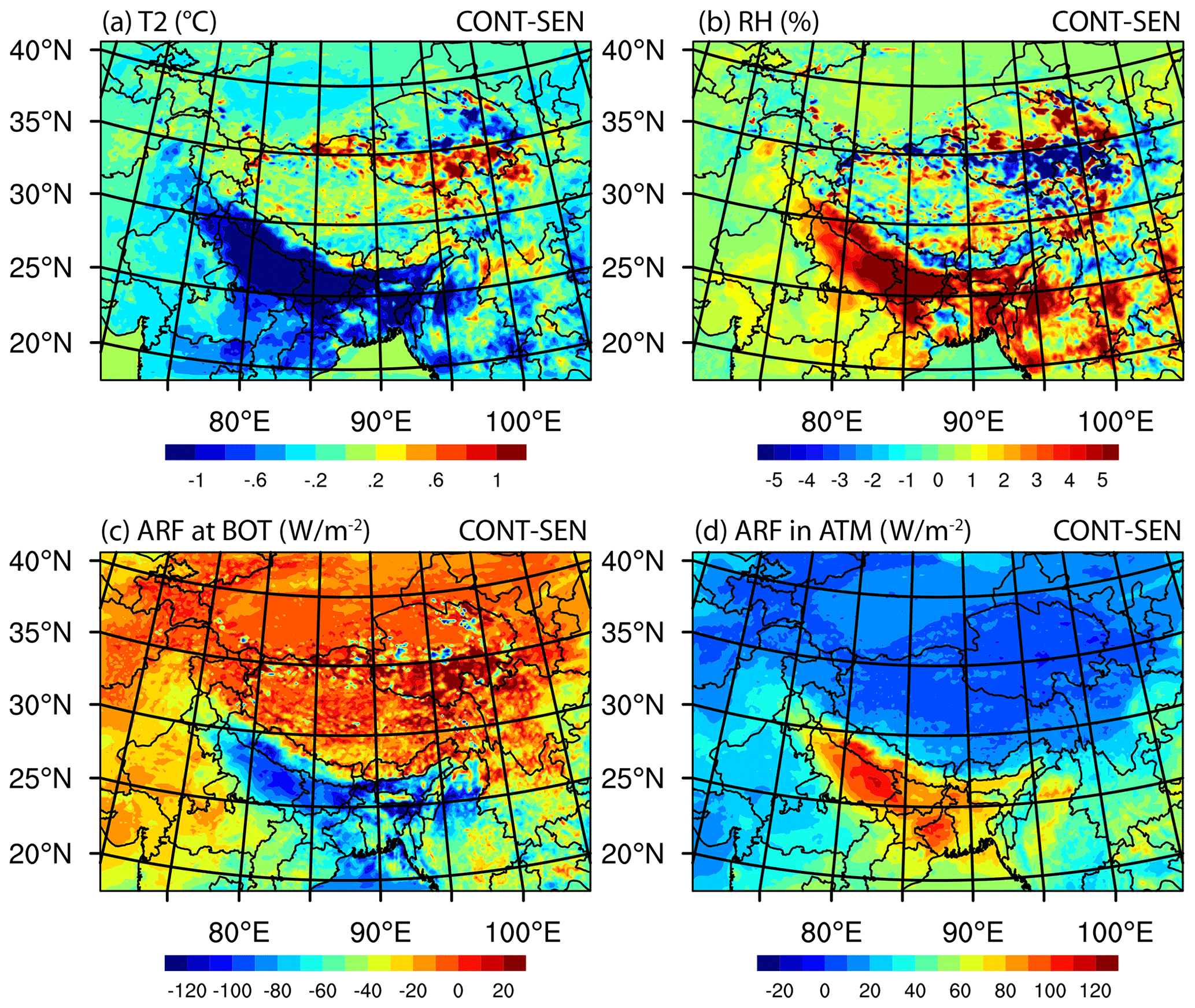
Figure 9 Spatial distributions of the aerosol-induced changes in (a) T₂ (^∘C), (b) RH2 (%), and the aerosol radiative forcing (ARF, W m⁻²) (c) at the bottom of the atmosphere (BOT) and (d) in the atmosphere (ATM) averaged for 09:00–20:00 BJT during the period from 27 April to 4 May 2016.

The ARF at the bottom of the atmosphere is negative over most parts of the study area except for the northern TP, where the ARF is positive and reaches up to 20 W m⁻² (Fig. 9c). The largest negative ARF observed occurred in northern South Asia and the Bay of Bengal, with values in the range of about −40 to −120 W m⁻² (Fig. 9c). Contrary to the spatial distribution of ARF at the bottom of the atmosphere, the ARF in the atmosphere is positive over most parts of the study area, with the largest ARF reaching up to 110 W m⁻² in South Asia (Fig. 9d). Thus, when affected by aerosols, the atmospheric stratification over the study area is expected to be more stable.

According to the above analysis, the aerosol-induced changes in meteorological conditions and ARF have a significant impact on atmospheric stability. The profile of the equivalent potential temperature (EPT) can be used to characterize the stability of the atmosphere. Figure S10 shows the aerosol-induced changes in the EPT profiles at 02:00, 08:00, 14:00, and 20:00 BJT averaged during the period from 27 April to 4 May in the southern TP and IGP. It can be seen that, overall, the impact of aerosols on the EPT is smaller over the southern TP, with values in the range of about 0.08–0.24 K, than over the IGP, with values in a range of about −1.6 to 3.2 K, because of the low aerosol concentrations in the southern TP and the high aerosol concentrations in the IGP. Specifically, at 08:00, 14:00, and 20:00 BJT, the EPT in the southern TP decreased with height in the lower and middle troposphere and increased with height above the middle troposphere (Fig. S10a). However, in the IGP, at 02:00 and 20:00 BJT, the EPT decreased with height below 550 hPa and increased with height above 550 hPa, while at 14:00 BJT, the EPT decreased with height below 650 hPa and increased with height between 650 and 550 hPa (Fig. S10b). Therefore, an obvious temperature inversion was detected in the troposphere over the southern TP and IGP during the severe aerosol pollution event.

Under a more stable atmosphere, the diurnal variation in the surface BC concentration from the control experiment with aerosol–meteorology feedback and the aerosol-induced changes in U₁₀ and PBLH over the southern TP and IGP are presented in Fig. 10. Overall, the surface BC concentration over the southern TP and IGP was high during 20:00–08:00 BJT in the nighttime but low during 08:00–20:00 BJT in the daytime. Over the southern TP, the aerosol-induced PBLH decreased by values of up to 55 m during 09:00–14:00 BJT and by 70 m during 18:00–20:00 BJT, while no obvious change in PBLH was observed at other times of the day (Fig. 10a). In the IGP, the aerosol-induced PBLH decreased during 10:00–20:00 BJT in the daytime, with the largest decrease of 1700 m occurring at 20:00 BJT (Fig. 10b). A lower PBLH constrains the pollutants to diffuse in the vertical direction and is conducive to the accumulation of pollutants near the ground. The aerosol-induced U₁₀ increased in the southern TP, with the maximum increase of 0.2 m s⁻¹ appearing at 19:00 BJT (Fig. 10a). In the IGP, the aerosol-induced U₁₀ decreased, with the largest decrease of 0.7 m s⁻¹ appearing at 20:00 BJT (Fig. 10b). Therefore, the aerosol induced significant changes in the meteorological conditions in the southern TP and IGP during this severe aerosol pollution event.

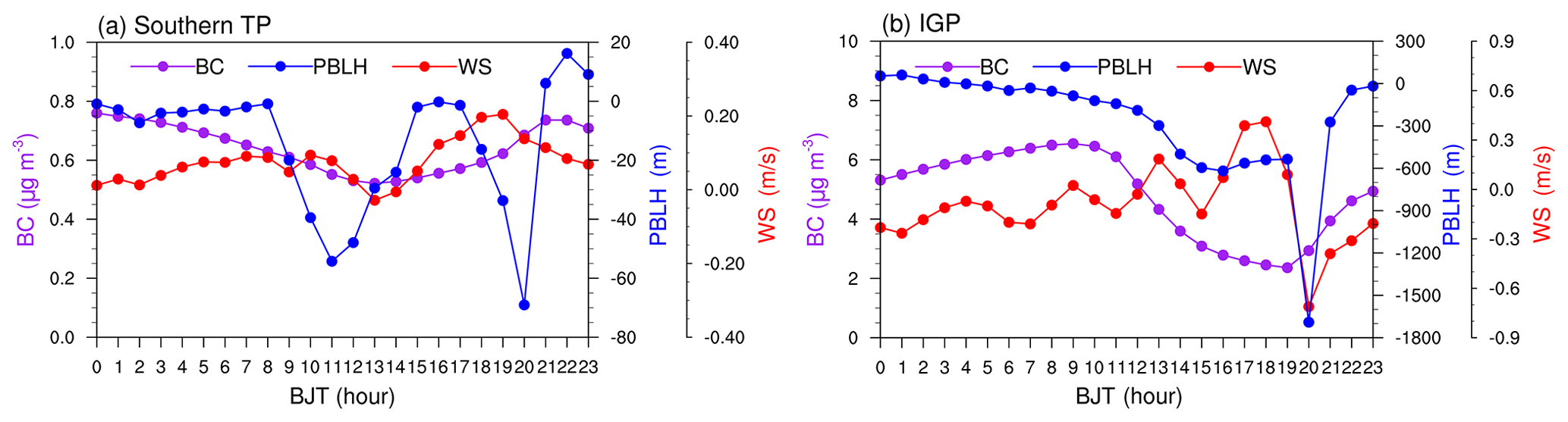
Figure 10 Diurnal variation in the surface BC concentration (µg m⁻³) from the control experiment with aerosol–meteorology feedback (solid purple line) and aerosol-induced diurnal changes in the 10 m wind speed (solid red line, WS, m s⁻¹) and PBLH (solid blue line, m) averaged for (a) the southern TP and (b) the IGP during the period from 27 April to 4 May 2016.

The aerosol-induced changes in meteorological conditions have an important effect on the surface BC concentration, which eventually exerts a potential influence on aerosol pollution as well as weather and climate (Menon et al., 2002). Figure 11a and b show the hourly surface BC concentration from a sensitive experiment without aerosol–meteorology feedback and the impact of aerosol-induced changes in meteorological variables on the hourly surface BC concentration averaged over the southern TP and IGP during the period from 20 April to 1 May. The corresponding diurnal cycles during the most polluted period from 27 April to 4 May are shown in Fig. 11c and d. Here the change in percentage is defined as the difference in surface BC concentration from CONT with aerosol-meteorology feedback and SEN without aerosol-meteorology feedback divided by the surface concentration from SEN without aerosol-meteorology feedback. It can be seen that the aerosol-induced changes in meteorological conditions lead to a decrease in the surface BC concentration of up to 0.16 µg m⁻³ (50 %) in the southern TP. However, in the IGP, the aerosol-induced changes in meteorological conditions result in an increase in the surface BC concentration of up to 2.2 µg m⁻³ (75 %). Moreover, the higher the surface BC concentration, the greater the variation in the surface BC concentration induced by the meteorological conditions. It should be noted that the time when the maximum decrease or increase in the surface BC concentration occurs is not the time when the maximum surface BC concentration occurs. The diurnal changes in surface BC concentration during the most polluted period from 27 April to 4 May over the southern TP indicate that the surface BC concentration is high during 20:00–07:00 BJT in the nighttime and low during 08:00–19:00 BJT in the daytime, with the lowest concentration of 0.6 µg m⁻³ observed at 12:00 BJT. The changes in meteorological conditions lead to a reduction in the surface BC concentration over the southern TP, with the reduction primarily occurring during 11:00–19:00 BJT in the daytime and the largest reduction of 0.06 µg m⁻³ (12 %) appearing at 15:00 BJT. The corresponding diurnal changes in the IGP reveal that the surface BC concentration is high during 23:00–12:00 BJT and low during 13:00–22:00 BJT. The changes in the meteorological conditions result in an increase in the surface BC concentration, with a relatively large increase of about 0.7–1.1 µg m⁻³ occurring during 20:00–13:00 BJT. Therefore, the changes in meteorological conditions enhance the diurnal variation in the surface BC concentration by decreasing the surface BC concentration in the southern TP and increasing the surface BC concentration in the IGP.

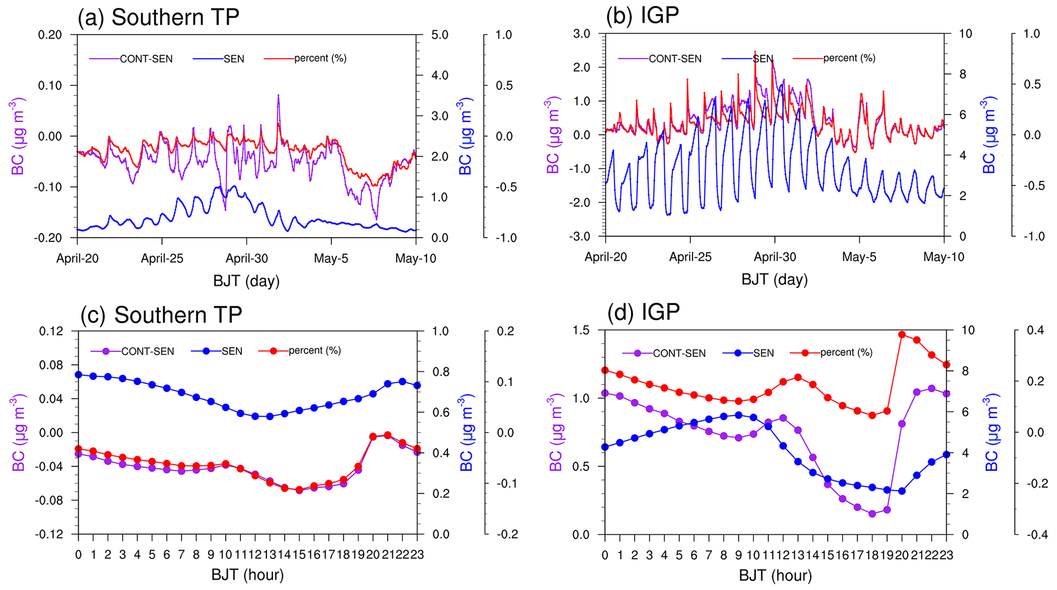
Figure 11 Time series of hourly surface BC concentrations from SEN (solid blue line) averaged for (a) the southern TP and (b) the IGP during the period from 20 April to 10 May 2016 and the corresponding diurnal changes (solid blue line) averaged (c) for the southern TP and (d) the IGP during the period from 27 April to 4 May 2016. The solid purple line denotes the change in the surface BC concentration induced by the meteorological conditions. The solid red line indicates the corresponding change in percentage terms compared to the surface BC concentration from the results of SEN.

Figure S11 shows the impact of aerosol-induced changes in meteorological conditions on the spatial distribution of the surface BC concentration averaged during 09:00–20:00 BJT on 27 April–4 May. Consistent with Fig. 11, the maximum increase in surface BC concentration induced by the changes in meteorological conditions occurs in the IGP (northwestern South Asia), with values greater than 1 µg m⁻³. The corresponding surface BC concentration change in percentage terms is also higher in northwestern South Asia, with values of up to 30 %, and is lower in the southeastern TP, with values of below 30 % (Fig. S11b). Taken together, aerosols result in significant changes in meteorological conditions in the southern TP and IGP, including an obvious decrease in PBLH and U₁₀ along with a more stable atmosphere in the IGP, and a decrease in PBLH but an increase in U₁₀ accompanied by a stable atmosphere in the southern TP. In addition, the aerosol-induced changes in meteorological conditions have a substantial influence on the surface aerosol concentration. For instance, in the IGP, the changes in meteorological conditions induced by aerosols are conducive to the accumulation of aerosols, thereby contributing to the formation of a severe aerosol pollution event. Consequently, a positive feedback mechanism exists between aerosol concentration and aerosol-induced meteorological conditions in the IGP. However, although it is one of the major source regions for the aerosols over the TP, the aerosol-induced changes in meteorological conditions in the IGP are not favorable for aerosol transport to the southern TP.

3.5 Impact of aerosol–meteorology feedback on the transboundary transport flux of BC

As discussed above, during the severe aerosol pollution event, northwestern South Asia contributed more BC to the TP via cross-Himalayan transport, and the largest BC transport flux occurred at a mountain valley in the western Himalayas. Moreover, aerosol–meteorology feedback has a substantial effect on the surface BC concentration over the southern TP and IGP. Yet, the effect the aerosol–meteorology feedback has on the transboundary transport flux of BC remains unclear and deserves further investigation. Therefore, this section aims to demonstrate the impact of aerosol–meteorology feedback on the transboundary transport flux of BC during the severe aerosol pollution event. Figure 12 shows the difference in longitude–height cross sections of the difference in BC transport flux along the cross line (shown as the dashed blue line in Fig. 2) between the simulations with and without aerosol–meteorology feedback at 15:00 and 03:00 BJT averaged for the period from 27 April to 4 May 2016. It can be seen that, during the daytime in the central and western Himalayas (75–90^∘ E), overall, the aerosol–meteorology feedback increases the BC transport flux towards the TP at a height of about 6–7 km but decreases the BC transport flux at heights below 6 km; however, in the eastern Himalayas (90–98^∘ E), the aerosol–meteorology feedback decreases the BC transport flux exported from the TP. During the nighttime, from 80 to 87^∘ E in the central Himalayas, the aerosol–meteorology feedback increases the BC transport flux towards the TP at a height of about 6–7 km but decreases the BC transport flux at heights below 6 km; however, from 87 to 94^∘ E in the eastern Himalayas, the aerosol–meteorology feedback decreases the BC transport flux towards the TP at heights below 7 km, and from 94 to 98^∘ E, the aerosol–meteorology feedback decreases the BC transport flux exported from the TP.

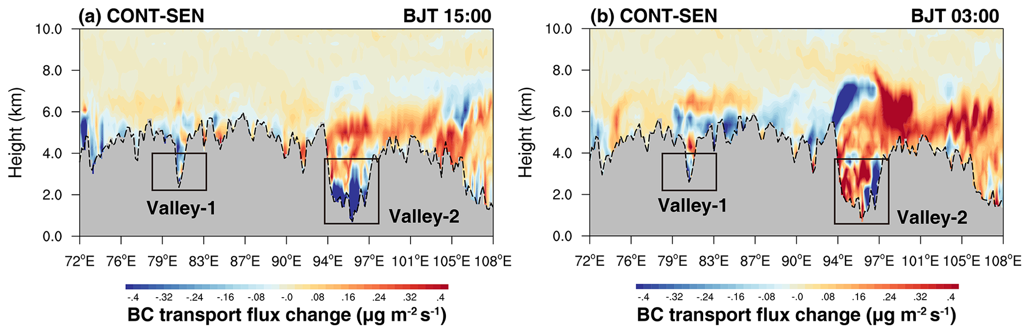
Figure 12 Difference in longitude–height cross sections of the difference in BC transport flux along the cross line (shown as the dashed blue line in Fig. 2) between the simulations with and without aerosol–meteorology feedback at 15:00 and 03:00 BJT averaged for the period from 27 April to 4 May 2016. The difference in PBLH along the cross section is shown here as the dashed black line.

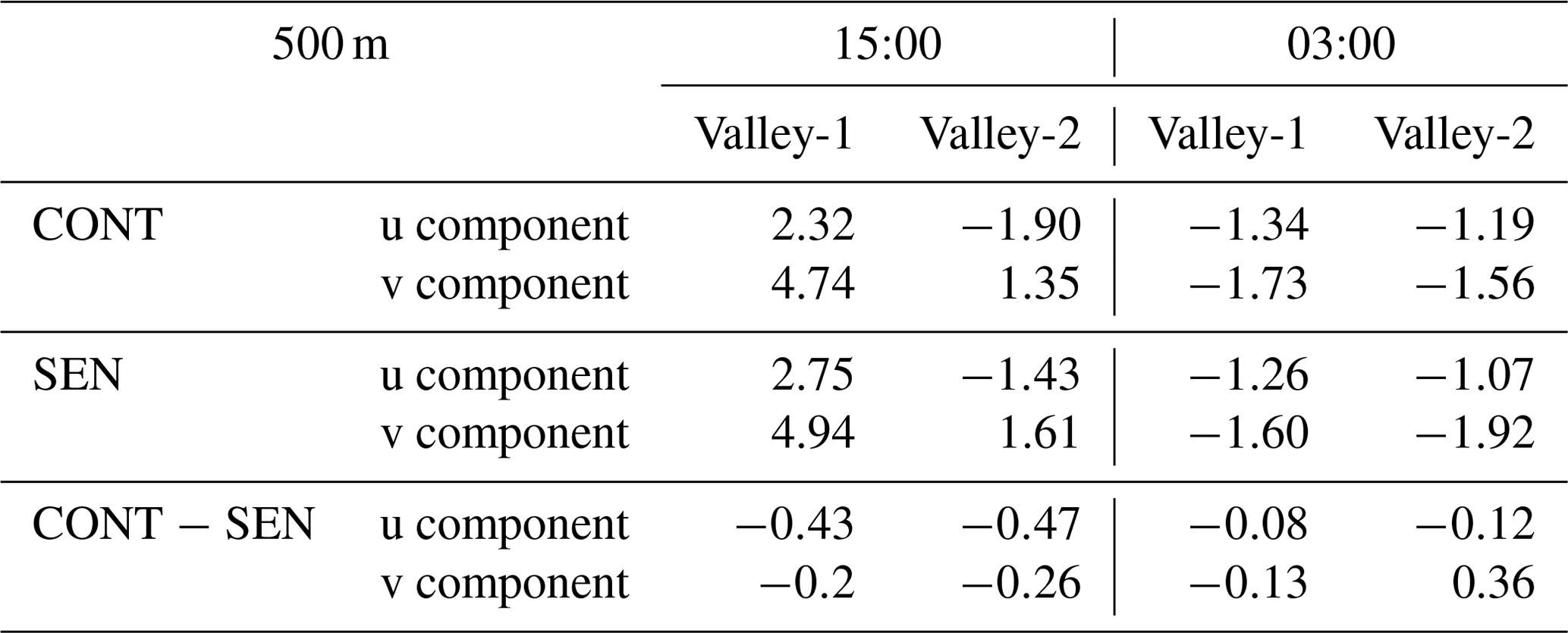
In addition, by analyzing the impact of aerosol–meteorology feedback on the BC transport flux at two typical mountain valley channels, it is found that, at valley-1, the feedback decreases the BC transport flux towards the TP during the daytime and nighttime, and at valley-2, the feedback decreases the BC transport flux towards the TP during the daytime and reduces the BC transport flux away from the TP during the nighttime. To better understand the effect of the aerosol–meteorology feedback on the BC transport flux at the two typical mountain valley channels valley-1 and valley-2, we investigated the mean zonal and meridional wind speeds within 500 m a.g.l. at both valleys during the daytime and nighttime from 27 April to 4 May 2016 (Table 2) from simulations with and without aerosol–meteorology feedback. It is found that, during the daytime, a westerly and a southerly prevail at valley-1 but an easterly and a southerly prevail at valley-2; during the night, an easterly and a northerly prevail at both valleys in both experiments. Specifically, at valley-1, the differences in zonal and meridional wind speeds between the simulations with and without aerosol–meteorology feedback at 15:00 and 03:00 BJT averaged for the period from 27 April to 4 May 2016 show that, during the daytime, the aerosol–meteorology feedback decreases the westerly and southerly wind speeds overall, resulting in a decreased BC transport flux towards the TP; during the night, the aerosol–meteorology feedback leads to increased easterly and northerly wind speeds, strengthening the BC transport flux away from the TP. The corresponding results at valley-2 indicate that, during the daytime, the aerosol–meteorology feedback increases the easterly wind speed but decreases the southerly wind speed, resulting in a decreased transport flux of BC towards the TP; during the night, the aerosol–meteorology feedback increases the easterly wind speed but decreases the northerly wind speed, leading to reduced BC transport flux away from the TP. It should be emphasized that the impacts of the aerosol–meteorology feedback on the BC transport flux averaged within 2000 m a.g.l. at the two typical mountain valley channels (Table S3) are consistent with the corresponding impacts when the BC transport flux is averaged within 500 m a.g.l.

Table 2 The mean zonal and meridional wind speeds at two typical valley channels within 500 m a.g.l. at 15:00 and 03:00 BJT averaged for the period from 27 April to 4 May 2016 from the CONT and SEN experiments. The differences in zonal and meridional wind speeds between the two experiments are also shown. A positive value denotes a westerly or a southerly and a negative value denotes an easterly or a northerly.

Similarly, to analyze the impact of aerosol–meteorology feedback on the vertically integrated transboundary transport flux of BC, the difference between the longitudinal distributions of integrated BC transport flux along the cross line (shown as the dashed blue line in Fig. 2) from the simulations with and without aerosol-meteorology feedback is shown in Fig. 13. As can be seen, with the aerosol–meteorology feedback, the integrated BC transport flux from central and western Himalayas (to the west of 88^∘ E) to the TP decreases overall; however, in the eastern Himalayas, the aerosol–meteorology feedback reduces the integrated transport flux of BC away from the TP (Fig. 13). Therefore, the aerosol–meteorology feedback exerts a substantial effect on the cross-Himalayan transport flux of BC.

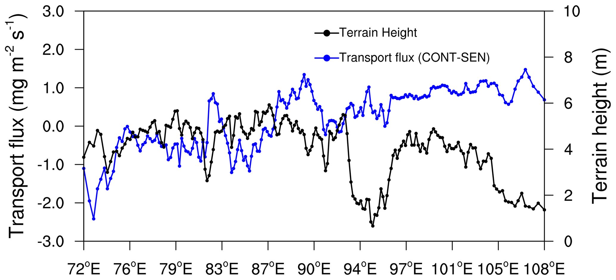
Figure 13 Difference between the longitudinal distributions of vertically integrated BC transport flux along the cross section in Fig. 2 from simulations with and without aerosol–meteorology feedback. The black line represents the terrain height.

4 Conclusions

The worst aerosol pollution episode ever recorded over the TP occurred during the period from 20 April to 10 May 2016. The largest observed AODs at the reference sites of Nam Co and QOMS were 0.65 and 0.42, respectively. In this paper, the meteorological causes of this severe aerosol pollution event, the BC transport flux, and the aerosol–meteorology feedback as well as its effect on BC transport flux during this severe aerosol pollution event were investigated by using observational and reanalysis datasets and WRF-Chem simulation. By analyzing the evolution of weather maps at 500 hPa over the study area during this severe aerosol pollution event, it was found that the plateau vortex plays a critical role in increasing the aerosol concentration in the inland of the TP. However, in the southern TP, the increase in aerosol concentration can be attributed to long-range transport by the southwesterly airflow in front of the trough.

Given the acceptable performance of the WRF-Chem model in simulating meteorological conditions and aerosols, we estimated the cross-Himalayan transport flux of BC. The results show that, in the central and western Himalayas, BC is imported into the TP during the day and night. However, in the eastern Himalayas, BC is imported into the TP during the day but exported slightly from the TP during the night; to the east of ∼98^∘ E, BC is transported away from the TP during the day and night. The vertically integrated transport flux of BC along the cross line during the aerosol pollution event exhibits a decreasing trend overall from west to east, with the largest vertically integrated BC transport flux of 20.8 mg m⁻² s⁻¹ occurring at the deepest mountain valley in southwestern TP.

By designing experiments with or without aerosol–meteorology feedback, the feedback between aerosol and meteorology over the southern TP and IGP during this severe aerosol pollution event was investigated. It was found that during the most polluted period from 27 April to 4 May, aerosols led to a slight change in surface air temperature in the southern TP but a significant decrease in surface air temperature, with values in the range of 0.5–1.7 ^∘C, in the IGP. Vertically, in the southern TP, the largest temperature increase induced by aerosols occurred in the middle troposphere; however, in the IGP, the aerosol-induced temperature decreased near the surface but increased in the middle troposphere. Spatially, the ARF was negative at the bottom of the atmosphere but positive in the atmosphere. As a result, the atmospheric stratification over the study area was more stable. Additionally, affected by aerosols, U₁₀ increased in the southern TP, with the largest increase of 0.2 m s⁻¹ appearing at 19:00 BJT, while U₁₀ decreased in the IGP, with the largest decrease of 0.7 m s⁻¹ appearing at 20:00 BJT. In respect to the PBLH, aerosols led to a decrease of 55 m in the PBLH during 09:00–14:00 BJT and of 60 m during 17:00–20:00 BJT in the southern TP, whereas a decrease in PBLH resulting from aerosols mainly occurred during 10:00–20:00 BJT in the daytime in the IGP, with the largest decrease of 1300 m detected at 20:00 BJT. Therefore, aerosols exert an important effect on meteorological conditions. By contrast, aerosol-induced changes in meteorological conditions can lead to a decrease in the surface BC concentration of up to 0.16 µg m⁻³ (50 %) in the southern TP and an increase in the surface BC concentration of up to 2.2 µg m⁻³ (75 %) in the IGP.

By investigating the impact of aerosol–meteorology feedback on the BC transport flux, it was found that, with the aerosol–meteorology feedback, the vertically integrated transport flux of BC from the central and western Himalayas to the TP decreases overall; however, in the eastern Himalayas, the aerosol–meteorology feedback reduces the vertically integrated transport flux of BC away from the TP. In particular, the corresponding results at two typical mountain valley channels in the southwestern and southeastern TP reveal that the aerosol–meteorology feedback decreases the import of BC towards the TP at the mountain valley channel in the southwestern TP during the daytime and nighttime, while at the mountain valley channel in the southeastern TP, the feedback decreases the import of BC towards the TP during the daytime and reduces the BC transport flux away from the TP during the nighttime.

Based on a severe aerosol pollution event, this study investigated the potential impact of aerosol–meteorology feedback on the transport of BC to the southern TP for a relatively short period. Similar studies that instead focus on a long period of BC transport are necessary to examine whether the results obtained in this study are universal. In addition, a finer grid resolution of the model domain and an improvement in the spatiotemporal resolution of the emission inventory is needed to minimize the model's biases caused by the TP's particularly complex topography. Furthermore, the results of this study show for the first time that the aerosol–meteorology feedback plays a substantial role in the transboundary transport of aerosols to the TP. Aerosols over the TP exert an important effect on the convective system over the TP (Zhao et al., 2020; Zhou et al., 2017). In the monsoon season, the convective activity is very vigorous over the TP. The aerosols that undergo transboundary transport along the slope from the foothill up to the TP via aerosol–meteorology feedback may also play a role. The potential impacts of aerosols on the regional climate over the TP deserve in-depth investigation using a high-resolution model that can resolve the complex topography of the TP.