the Creative Commons Attribution 4.0 License.
the Creative Commons Attribution 4.0 License.
 | 25 Jul 2024
Upper-atmosphere responses to the 2022 Hunga Tonga–Hunga Ha′apai volcanic eruption via acoustic gravity waves and air–sea interaction
Qinzeng Li
Jiyao Xu
Aditya Riadi Gusman
Hanli Liu
Wei Yuan
Weijun Liu
Yajun Zhu
A multi-group of strong atmospheric waves (wave packet nos. 1–5) over China associated with the 2022 Hunga Tonga–Hunga Ha′apai (HTHH) volcano eruptions were observed in the mesopause region using a ground-based airglow imager network. The horizontal phase speed of wave packet nos. 1 and 2 is approximately 309 and 236 m s−1, respectively, which is consistent with Lamb wave L0 mode and L1 mode from theoretical predictions. The amplitude of the Lamb wave L1 mode is larger than that of the L0 mode. The wave fronts of Lamb wave L0 and L1 below the lower thermosphere are vertical, while the wave fronts of L0 mode tilt forward above the lower atmosphere, exhibiting internal wave characteristics which show good agreement with the theoretical results. Two types of tsunamis were simulated; one type of tsunami is induced by the atmospheric-pressure wave (TIAPW), and the other type of tsunami is directly induced by the Tonga volcano eruption (TITVE). From backward ray-tracing analysis, the TIAPW and TITVE were likely the sources of wave packet nos. 3 and 4–5, respectively. The scale of tsunamis near the coast is very consistent with the atmospheric AGWs observed by the airglow network. The atmospheric gravity waves (AGWs) triggered by TITVE propagate nearly 3000 km inland with the support of a duct. The atmospheric-pressure wave can directly affect the upper atmosphere and can also be coupled with the upper atmosphere through the indirect way of generating a tsunami and, subsequently, tsunami-generating AGWs, which will provide a new understanding of the coupling between ocean and atmosphere.
- Article
(12373 KB) - Full-text XML
- BibTeX
- EndNote


Hunga Tonga–Hunga Ha′apai (HTHH) volcano, which erupted at 04:14:45 UT on 15 January 2022, produced the largest volcanic eruption in terms of the energy release of a single event since the Krakatoa volcanic eruption (Symons, 1888) in 1883. This volcanic eruption triggered broad-spectrum atmospheric disturbances (Adam, 2022; Duncombe, 2022; Wright et al., 2022), including Lamb waves (Zhang et al., 2022), acoustic waves, gravity waves (GWs) (Liu et al., 2022), and shock waves (Astafyeva et al., 2022). In addition, the traveling ionospheric disturbances (TIDs) caused by this volcanic eruption have also been reported (Themens et al., 2022; Lin et al., 2022).
Lamb waves are external waves propagating along Earth's surface at the speed of sound (Beer, 1974). They are non-dispersive or nearly non-dispersive (Francis, 1973) and can propagate horizontally over long distances. A Lamb wave mainly occupies the troposphere, and its perturbation pressure decays exponentially with height (Yeh and Liu, 1974). The Lamb waves excited by the Tonga volcano eruptions went around the Earth several times (Amores et al., 2022; Duncombe, 2022). Sepúlveda et al. (2023) found that the wind field strongly affects the morphology and propagation of a Lamb wave. Liu et al. (2023) reproduced the Lamb wave L0 and L1 modes consistently with theoretical predictions (Francis, 1973) using the high-resolution Whole Atmosphere Community Climate Model with the thermosphere/ionosphere extension (WACCM-X). Li et al. (2023) identified the Lamb wave L1 mode using phase-leveling amplitude technology based on a global navigation satellite system (GNSS) total electron content (TEC). Poblet et al. (2023) reported that the strong perturbations in the meteor radar horizontal wind field over South America are caused by the Lamb wave L1 mode associated with the 2022 HTHH volcano eruption.
Acoustic gravity waves (AGWs) are mechanical waves in compressible fluids in a gravity field (Gossard and Hooke, 1975). If the frequencies are much larger than the buoyancy frequency, then AGWs tend towards an acoustic wave mode; when the frequency is much smaller than the buoyancy frequency, then the fluid can be considered incompressible, and the AGWs tend towards internal GWs mode. The term “acoustic gravity waves” is usually used when restoring forces due to both gravity and compressibility is important. AGWs are known to play a significant role in the coupling between the atmosphere or ionosphere and the ocean (Press and Harkrider, 1962; Harkrider and Press, 1967; Donn and Balachandran, 1981; Azeem et al., 2017). Atmospheric-pressure waves are mechanical waves that are related to the density of the atmosphere. Compression and expansion are the high-pressure and low-pressure regions of motion in a medium.
The 2022 HTHH volcano eruption triggered tsunamis that affected the whole world (Carvajal et al., 2022; Ghent and Crowell, 2022). Conventional tsunamis are typically generated by localized sea surface displacements caused by sources such as earthquakes and volcanoes, similar to the tsunamis directly induced by the 2022 Tonga volcano eruption (TITVE). Another type of tsunami is induced by an atmospheric-pressure wave (TIAPW) (Kubota et al., 2022; Gusman et al., 2022). Tsunamis can generate upward-propagating AGWs through the water–air interface and propagate to the thermosphere/ionosphere (Hines, 1972; Peltier and Hines, 1976; Hickey et al., 2009, 2010; Occhipinti et al., 2013; Vadas et al., 2015; Laughman et al., 2017; Nishikawa et al., 2022; Pradipta et al., 2023). Using the red line airglow imager, Makela et al. (2011) detected an airglow disturbance in Hawaii that arrived 1 h earlier than the tsunami generated by the 11 March 2011 Tohoku earthquake. Also using the red line airglow, Smith et al. (2015) observed a tsunami and GWs almost simultaneously in Chile. Inchin et al. (2020) used a three-dimensional (3-D) numerical model to simulate the atmospheric AGWs generated by a tsunami. They found that bathymetry variations significantly affected the tsunamis and the AGWs excited by tsunamis, leading to their nonlinear evolution process. More recently, Inchin et al. (2022) performed the numerical simulations of mesopause airglow radiation fluctuations induced by tsunami-generated AGWs and found that large-scale tsunamis can cause detectable and quantitative disturbances of mesopause airglow through AGWs.
As far as we know, the research on the impact of tsunami-induced atmospheric AGWs on the atmosphere and ionosphere shown above is all related to conventional tsunamis. There are only two rare studies on the ground-based airglow observations of AGWs caused by this conventional tsunami, and both are limited to red line observations (Makela et al., 2011; Smith et al., 2015). However, the observation of tsunami-induced AGWs in the mesopause region observed by ground-based airglow imaging has never been reported. In this study, we first reported the propagation characteristics of the AGWs generated by the tsunamis triggered by the 2022 HTHH volcano eruptions in the mesopause region using the ground-based airglow imager observation network. We then focus on the coupling process of atmospheric-pressure waves triggering tsunamis, and then we look at tsunamis generating atmospheric AGWs through the air–water–air coupling process in the far-field area of the 2022 HTHH volcano eruption.
2.1 Multi-layer airglow imager network
A multi-layer airglow observation network (Xu et al., 2021) was built to study atmospheric disturbances excited by severe weather events, such as thunderstorms (Xu et al., 2015), typhoons (Li et al., 2022), and volcanic activities. Figure 1 shows the distribution of the multi-layer airglow observation network station. The multi-layer airglow observation network mainly includes a hydroxyl radical (OH) airglow network, which has been used to observe the airglow layer at the height of 87 km; an atomic oxygen emission (OI) airglow network has been used to observe the airglow layer at the height of 250 km. In addition, there were 557 nm airglow and Na airglow imagers installed at some stations, such as Xinglong station (40.4° N, 117.6° E) and Lhasa (29.7° N, 91.0° E). The airglow network can provide observations with a high temporal and spatial resolution. The time resolution of an OH airglow imager is 1 min, while the resolution of the OI 557 nm and OI 630 nm airglow imager is 3 min, respectively. The spatial resolution of the airglow imager at the airglow layer is not uniform. The resolutions of OH, OI 557 nm, and OI 630 nm airglow in the zenith direction are 0.27, 0.29, and 0.77 km, respectively, while in the zenith angle of 60° the resolutions are 1.01 (OH), 1.11 (OI 557 nm), and 2.65 km (OI 630 nm), respectively.
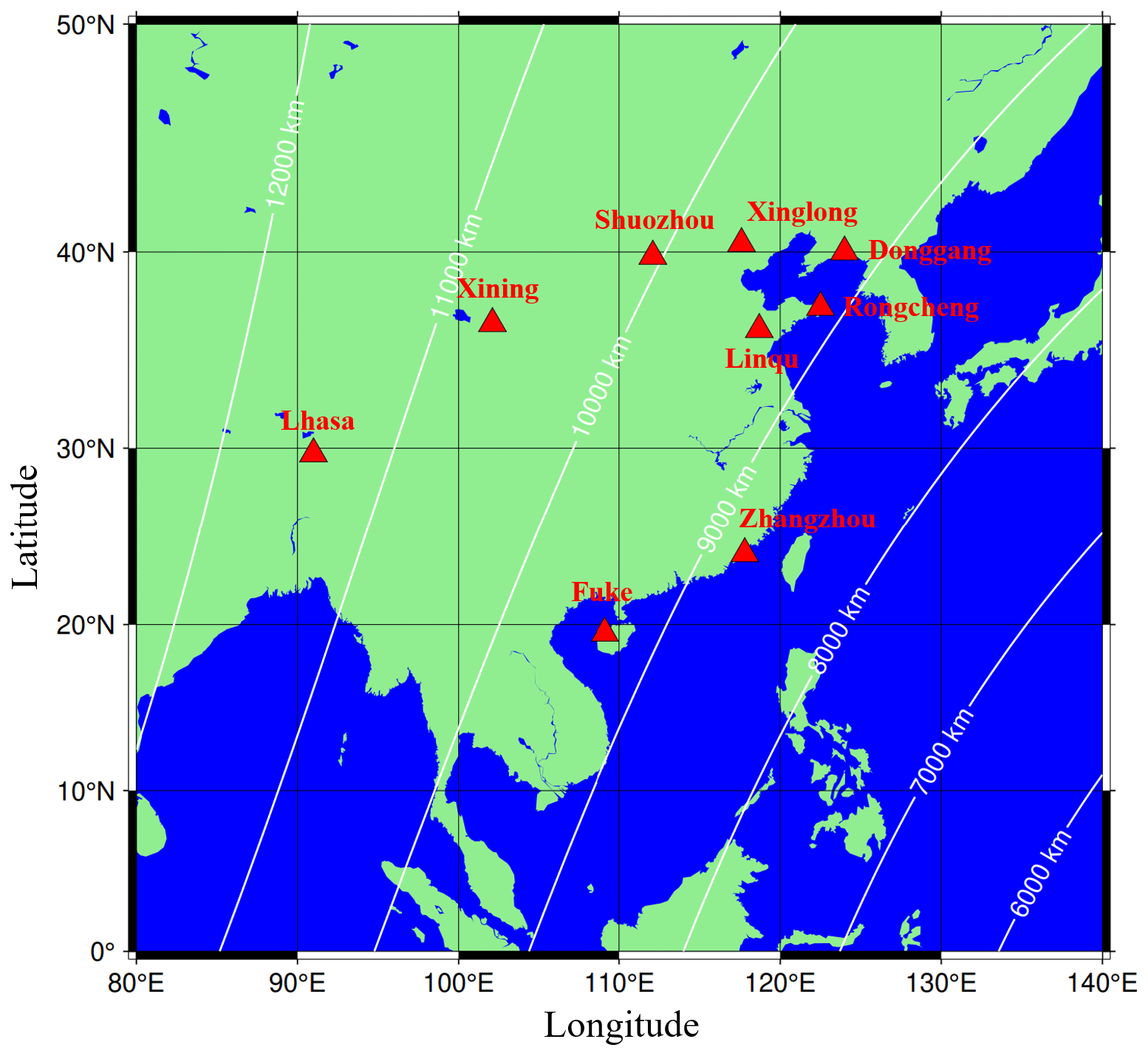
Figure 1The distribution of airglow network stations, along with the large circle centered on the Tonga volcano and its radius length, is marked in the figure.
2.2 Spectral analysis of atmospheric wave parameters
The airglow image was calibrated with the help of standard star map (Garcia et al., 1997) and projected into geospatial space. The background radiation is removed by the time differential (TD) method (Swenson and Mende, 1994) to highlight atmospheric fluctuations. The atmospheric wave parameters (horizontal wavelength λh, observed horizontal phase speed c, and the relative intensity perturbation ) are extracted from the spectral analysis method. Figure 2c presents the two-dimensional cross-spectrum obtained from Fig. 2a and b. Zonal (kx) and meridional (ky) wave numbers are determined from the peak position of the spectra. The horizontal wavelengths λh are obtained from the expression of . The observed speeds c are calculated from the phase (φ) (Fig. 2d) at the maximum peak of the cross-spectrum as , where Δt is the time interval between the two TD images. The amplitudes of intensity perturbations were calculated by integrating the power surrounding the central peaks of the power spectrum. To eliminate noise, the energy of the wave spectrum should be greater than 10 % of the total spectrum (Tang et al., 2005).
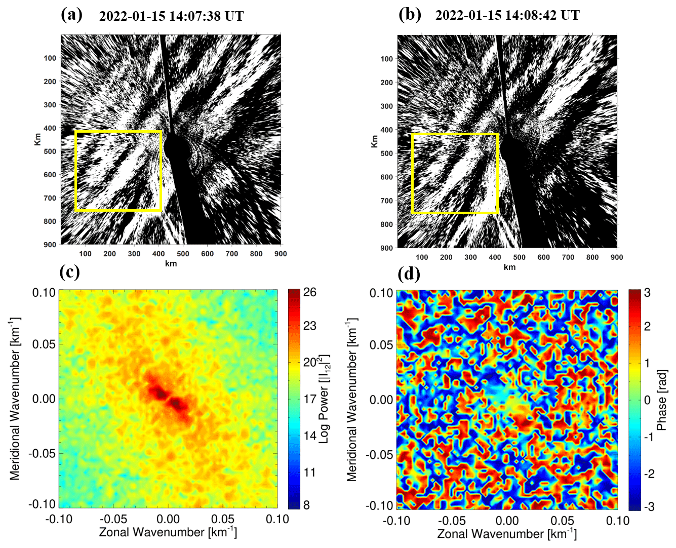
Figure 2The time difference images in panels (a) and (b) have been obtained from the Xinglong OH airglow imager on the night of 15 February 2022. Each image is projected on an area of 900 km×900 km. The (c) cross-spectrum and (d) phase obtained from the yellow box area in panels (a) and (b) using 2-D fast Fourier transform.
2.3 Tsunami simulation model
Tonga submarine volcano erupted on 15 January 2022 and generated tsunamis that were detected around the globe, particularly affecting the Pacific region. In this study, two types of tsunamis were simulated, namely conventional tsunami simulations and atmospheric-pressure, wave-induced tsunami simulations. The linear shallow-water equations in the spherical coordinate system are used to simulate the tsunamis from the localized source and atmospheric-pressure wave. The continuity equation of a linear shallow-water wave model with spherical coordinates is as follows:
where η is the free-surface elevation (m), d is the water depth (m), R is the Earth's radius (6 371 000 m), φ is longitude, and θ is colatitude.
While the momentum equations of the linear shallow-water wave model are
where u is the velocity along the lines of longitude (m s−1), v is the velocity along the lines of latitude, g is the gravitational acceleration (9.81 m s−2), p is the atmospheric pressure (Pa), ρ is the seawater density (1026 kg m−3), and f is the Coriolis coefficient. For the atmospheric-pressure wave-induced tsunami simulation, the moving pressure term is used as an input to the tsunami simulation momentum equation. The atmospheric-pressure wave model is based on the Eq. (1) in Gusman et al. (2022).
For the tsunami simulations from a localized source, a B-spline function (Koketsu and Higashi, 1992) is used below to represent the circular water uplift source at the volcano.
where
xk and xl stand for the coordinates of the knots along the x and y axes, h is the characteristic diameter of water uplift, r is the great-circle distance from the volcano eruption center, and and the other . In this study, the modeling domain covers the Pacific Ocean and some parts of the Indian Ocean and the Caribbean with a grid size of 5 arcmin. For detailed tsunami simulation algorithms, please refer to Gusman et al. (2022).
The models for the 2022 HTHH volcanic eruption used in this study was estimated and validated with observations at offshore DART stations around the Pacific Ocean in a previous study (Figs. 3 and 7 in Gusman et al., 2022).
2.4 Ray-tracing method
The following ray-tracing equations (Lighthill, 1978) describe the propagation path of AGWs.
where xi, ki, , (), and ω are the position vector, wavenumber vector, group speed, and intrinsic frequency, respectively.
Using the dispersion relation of acoustic gravity wave (Yeh and Liu, 1974), we can assess the vertical propagation state of AGWs. The dispersion relation is as follows:
where m is the vertical wave number, k is the horizontal wave number, cs the local speed of sound, is the intrinsic frequency, and u is the background wind speed in the direction of wave propagation from meteor radar observations and ERA5 (Hersbach et al., 2020). is the acoustic cutoff frequency, is the buoyancy frequency, g is the gravitational acceleration, and T is temperature from the Sounding of the Atmosphere using Broadband Emission Radiometry (SABER) instrument on the Thermosphere, Ionosphere, Mesosphere Energetics and Dynamics (TIMED) satellite. When ω>ωa or ω<ωb, m2>0, AGWs can propagate freely, whereas when , m2<0, the wave is evanescent.
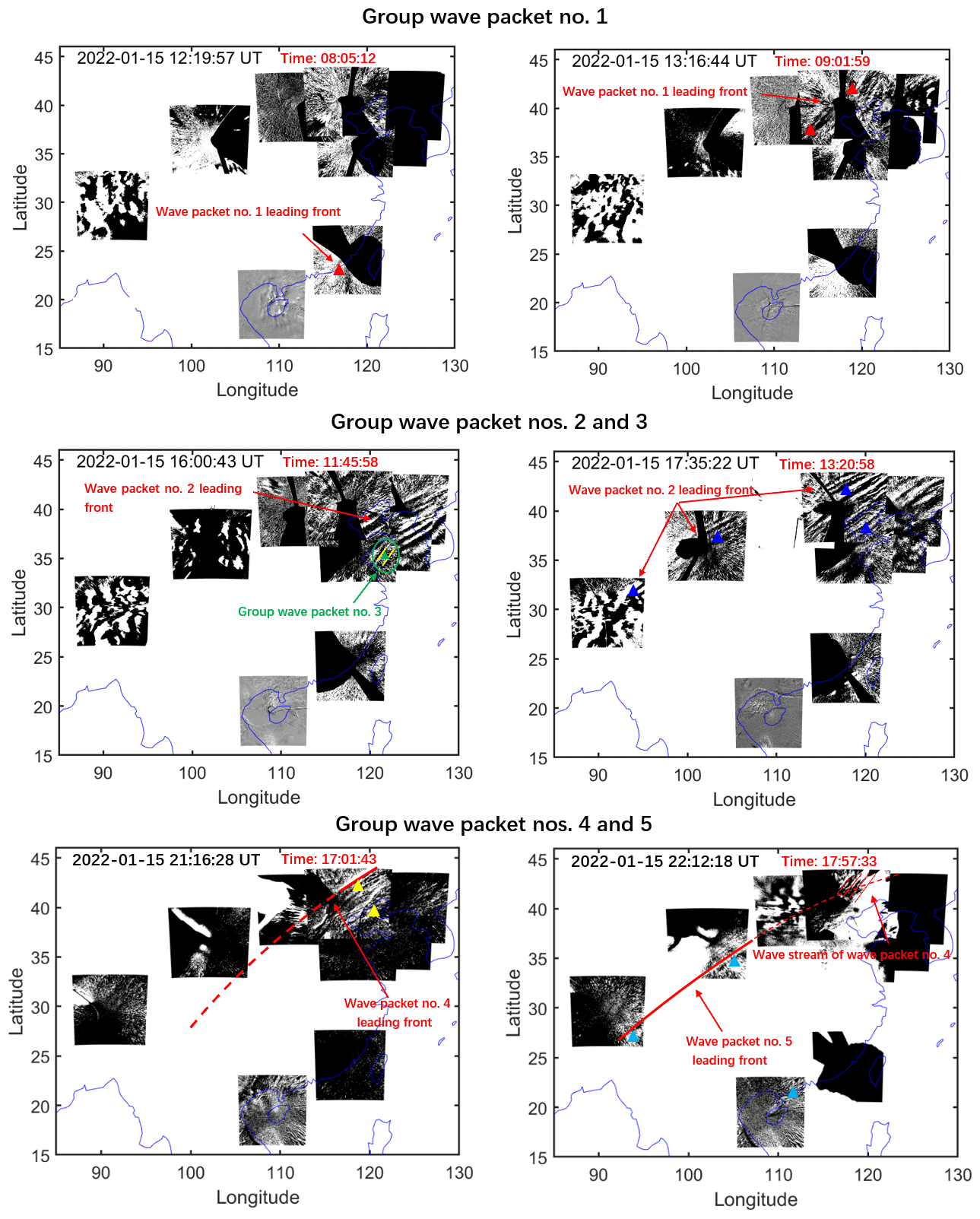
Figure 3Five strong group atmospheric waves associated with the Tonga volcano eruptions were observed in the mesopause region by the ground-based airglow network. Different colored triangles correspond to each wave event sampling point, while red, blue, green, yellow, and cyan correspond to wave packet nos. 1, 2, 3, 4, and 5, respectively. The red time markers in this figure and the following figure represent the lapse time since the volcano eruption.
3.1 Upper-atmospheric airglow responses to HTHH volcanic eruption via Lamb waves
Five groups of atmospheric waves (wave packet nos. 1–5) were observed in the mesopause region by the ground-based airglow network. Refer to the Supplement (https://doi.org/10.5446/66190; Li, 2024c) for the detailed wave propagation status. To eliminate random disturbances, we also made videos of 2 d before and after the volcanic eruption (https://doi.org/10.5446/s_1689; Li, 2024b). From the videos, it can be seen that the OH airglow layer was very calm during this period. Figure 3 shows wave packet no. 1 observed by the airglow imager network (top panels). Wave packet no. 1 entered the view of the airglow network approximately 8 h after the HTHH volcanic eruption (left panel of the top row). A total of 3 h after wave packet no. 1 entered the field of view, wave packet no. 2 was observed by the airglow network. The leading front of wave packet no. 2 has an uninterrupted continuous front, which almost covers the whole Chinese mainland (middle panels). Interestingly, we observed AGWs accompanying wave packet no. 2 (hereafter wave packet no. 3) over the northwestern region of the Yellow Sea (left panel of middle row). Wave packet no. 2 always keeps a stable state in the process of propagation and maintains a regular front when propagating over Lhasa station (29.7° N, 91.0° E). Wave packet no. 4 exhibits strong instability characteristics during propagation. Compared to the continuous leading front of wave packet no. 2, the fronts of wave packet nos. 4 and 5 are separated (bottom panels). We also found that wave packet no. 5 propagates more than 3000 km inland (propagating to the area west of 90° E).
Figure 4 shows the distribution of wave parameters for multi-group of atmospheric waves (wave packet nos. 1–5) from cross-spectral analysis. The phase speed of wave packet no. 1 leading front is approximately 309 m s−1. Wave packet no. 2 displays a slightly slower phase speed, with an average phase speed of 236 m s−1. The horizontal phase speeds of the group with wave packet nos. 3–5 are mainly distributed in the range of 200 to 215 m s−1, which is smaller than that of wave packet nos. 1–2. The horizontal wavelengths of these five grouped wave packets are mainly distributed in 80–105 km, while the observation periods are relatively small and mainly concentrated in 5.7–7.2 min. For amplitude, the average amplitude of the Lamb wave L1 mode (5.4 %) is higher than that of the Lamb wave L0 mode (3.2 %). Wave packet nos. 3, 4, and 5 have relatively small amplitudes, mainly distributed between 0.85 % and 1.25 %.
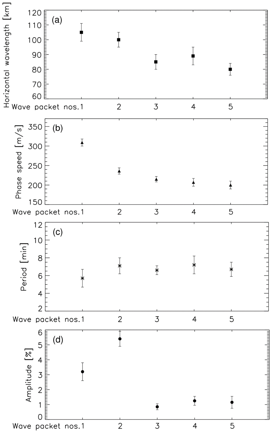
Figure 4Distribution of (a) horizontal wave wavelength, (b) phase speed, (c) period, and (d) amplitude parameters for a multi-group of atmospheric waves (wave packet nos. 1–5). The calculation of wave packet parameters comes from the average value of the wave passing through the sampling points in Fig. 3.
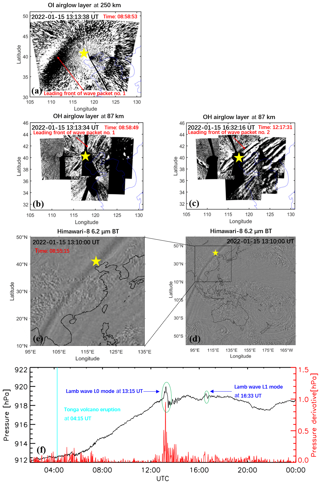
Figure 5(a) OI 630 nm airglow observation at 13:13:18 UT. OH airglow network observations when (b) wave packet no. 1 and (c) wave packet no. 2 pass through the zenith direction of Xinglong station at 13:13:34 and at 16:32:16 UT, respectively. (d, e) Himawari-8 6.2 µm brightness temperature at 13:10:00 UT. (f) The surface time series of surface pressure obtained from Xinglong station. The red line represents the time derivative of the pressure. The sudden change in air pressure at 13:15 UT indicates the arrival time of Lamb wave L0. A small disturbance of air pressure that occurs at 16:33 UT indicates the arrival time of Lamb wave L1. The yellow stars represent the location of Xinglong station.
The HTHH volcano eruption produced Lamb waves that propagated around the globe (Wright et al., 2022), causing sudden changes in surface pressure (Omira et al., 2022; Takahashi et al., 2023). Figure 5f shows the surface air pressure data of Xinglong station (40.4° N, 117.6° E). At 13:15 UT on 15 January 2022, the air pressure dropped sharply from 920 to 917.7 Pa, indicating that a Lamb wave had arrived at the surface of Xinglong station at 13:15 UT. A small disturbance of air pressure occurred at 16:33 UT. Figure 5e and d present the Himawari-8 6.2 µm brightness temperature at 13:10:00 UT (Otsuka, 2022). It can be seen that the leading front of Lamb wave L0 mode happens to pass through the zenith direction of Xinglong station. The time when wave packet no. 1 (Fig. 5b) and wave packet no. 2 (Fig. 5c) reach the zenith direction of Xinglong station from the OH airglow observation is 13:13:34 and 16:32:16 UT, which matches the time for surface pressure disturbances quite well. The phase speed of wave packet no. 1 leading front (∼309 m s−1) is very close to the speed of surface Lamb wave (L0 mode). From the Fig. 5, it can be seen that the phase of the Lamb wave L0 mode is almost vertical from the ground to the stratosphere and then to the mesosphere. Wave packet no. 2, with a slower phase speed (∼236 m s−1), is consistent with the Lamb wave L1 mode in theoretical predictions (Francis, 1973) and simulations from the WACCM-X model (Liu et al., 2023). However, at almost the same time, the wave front observed in the thermosphere (Video Supplement; https://doi.org/10.5446/66280; Li, 2024a) with a slightly faster phase speed of 342 m s−1 is nearly 550 km ahead of the wave front in the mesopause region in the horizontal propagation direction and ahead of time by approximately 30 min (Fig. 5a). This is in good agreement with theoretical and modeling results (Fig. 4 in Lindzen and Blake, 1972; Fig. 2 in Liu et al., 2023), which show that the wave fronts of the Lamb wave below the lower thermosphere are vertical and tilt forward above. As for Lamb wave L1 mode, the ground and mesopause region provide waveguide surfaces, resulting in maximum wave energy between the two layers, while the phase does not change with height (Francis, 1973).
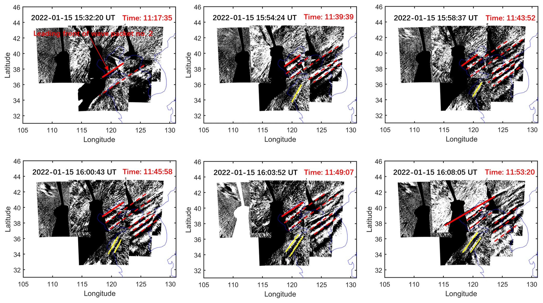
Figure 6The solid red lines indicate leading wave front of wave packet no. 2. The solid yellow lines mark wave packet no. 3; the lines are clearly not parallel to the wave fronts of wave packet no. 2.
As for why the observed Lamb wave L0 shape in the OH airglow layer is not a strong leading wave with much weaker trailing waves, this may be caused by the following factors. It is seen from model simulations that the wave amplitudes of the L0 and L1 modes are not uniform at the wave front. This non-uniformity becomes more pronounced in the upper atmosphere (e.g., Fig. 2 in Liu et al., 2023), probably as a result of the large variation in the background atmosphere propagation conditions. It is thus possible that over certain regions the trailing waves become comparable to the leading wave. It is also possible for the leading wave to gradually dissipate energy and become invisible during propagation by generating trailing waves. In addition, due to the smaller field of view of the airglow imager compared to satellite observations, some structures may be related to local fine structures, especially in the middle and upper layers, where many internal waves have significant amplitudes, which may be relatively more significant than Lamb waves.
As mentioned above, the amplitude of the Lamb wave L1 mode in the mesopause region is greater than that of the L0 mode, which may be due to the fact that the L1 mode is an internal wave below the mesopause (Liu et al., 2023). For an isothermal atmosphere, the Lamb wave L0 mode amplitude grows with altitude z as , where H is the scale height, , and γ is the ratio of specific heats (∼1.4). However, the amplitude of the internal GWs varies as . The amplitude of internal waves increases with height at a rate greater than that of surface modes.
Poblet et al. (2023) reported an observation of the Lamb wave L1 mode in the horizontal wind field of meteor radar, but they do not see the Lamb wave L0 mode and argue that the L0 mode is likely a higher-frequency wave and was averaged out. Stober et al. (2023, 2024) found that the anomalous peak signal in the meteor radar wind field cannot be completely determined to be caused by the Lamb wave generated by the Tonga volcanic eruption. On the one hand, meteor radar observations may have filtered out high-frequency Lamb waves. On the other hand, even if Lamb waves are observed in the upper atmosphere, there is still debate over whether they propagate directly to the upper atmosphere or through multi-step vertical coupling process described by Becker and Vadas (2018), Vadas and Becker (2018), and Vadas et al. (2018, 2023).
Figure 6 shows the time sequence of propagation image of wave packet no. 3. We found that with the propagation of wave packet no. 2, there is an AGW (wave packet no. 3) with a certain angle between its phase plane (solid yellow line) and the phase plane of wave packet no. 2. This implies that the source of wave packet no. 3 is different from that of wave packet no. 2. The horizontal wavelength of wave packet no. 3 near the coast is 84 ± 5 km.
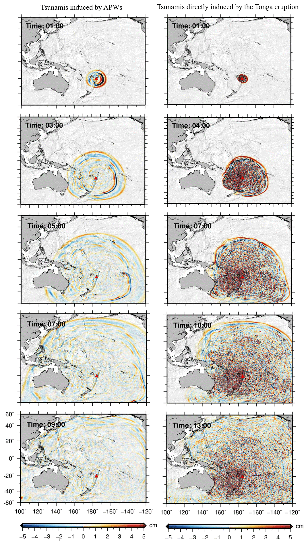
Figure 7Snapshots of simulated tsunamis induced by the atmospheric-pressure wave (left panels) and tsunamis directly induced by the Tonga volcano eruption (right panels).
3.2 Simulation of tsunami induced by HTHH volcano eruption
The 2022 HTHH volcano eruption triggered global atmospheric-pressure waves. The simulated atmospheric-pressure waves propagate at an approximate constant speed of 317 m s−1, and the amplitude decreases with the distance from the volcano (Gusman et al., 2022). Figure 7 shows snapshots of the TIAPW and TITVE simulation results. The leading TIAPW excited by the pressure disturbances travels at the same speed as the atmospheric-pressure wave and is followed by subsequent sea waves generated earlier in the atmospheric-pressure wave propagation which thereafter travels at the conventional tsunami propagation speed. Under a given pressure gradient, the discharge flux in the deep sea is much greater than that in shallow water. A deep-bathymetric feature such as the Kermadec–Tonga Trench can more effectively generate tsunami waves. The wave train following the leading wave traveling over the trench appears to be larger than those traveling in other directions. The propagation speed of TITVE from the shallow-water (long) wave approximation is (Salmon, 2014), where g is the gravitational acceleration, and H0 is the ocean depth. For seawater with a general depth of 4 km, the speed of shallow-water wave is about 200 m s−1. Therefore, the TIAPW is significantly faster than the TITVE. The amplitude of TITVE is greater than that of tsunamis generated by atmospheric-pressure waves. The wave train following the leading wave of TITVE exhibits finer structures with scales smaller than that of TIAPW. We found that the TIAPW arrived along the coast of the Chinese mainland about 4–5 h earlier than the TITVE.
3.3 Upper-atmosphere responses to HTHH volcanic eruption via air–sea interaction
Figure 8 shows the simulation results of TIAPW and TITVE near the coast of the Chinese mainland 11 h (15:15 UT) and 15 h (19:15 UT) after the volcanic eruption, respectively. Air pressure waves are not very efficient at directly exciting tsunamis in shallow water due to the weaker air–sea coupling (Gusman et al., 2022; Yamada et al., 2022). The Yellow Sea is quite shallow, so the amplitude of the leading of TIAPW is very small there. The leading wave is followed by subsequent waves with larger amplitudes, which propagate in the same direction as the leading wave but at the conventional tsunami speed (Gusman et al., 2022). We found that the TIAPW and TITVE on the continental shelf have shorter wavelengths compared with those in the deep ocean. When the tsunamis approached the coast of China, three groups of AGWs (wave packet nos. 3, 4, and 5) were observed by the airglow network. The time at which the AGWs entered the view of the airglow network was very close to the time when the Tonga tsunamis reached the coast of the Chinese mainland. Wave packet no. 3 entered the airglow network at 15:30 UT, and wave packet nos. 4–5 entered the airglow network at 19:40 UT. This strongly suggests that wave packets detected by the airglow network are correlated to the tsunamis near the coast. We found that as the tsunamis approached the coast of China, they diffracted between Taiwan and the Philippines and became discontinuous. And wave packet nos. 4 and 5 that we observed were also discontinuous, which further confirms the correlation between wave packet nos. 4–5 and discontinuous tsunamis. We estimate that the average wavelength of TIAPW near the coast of the Yellow Sea is approximately 82 ± 4 km, which is very consistent with the horizontal wavelengths of the atmospheric AGWs observed by the airglow network, as mentioned above (84 ± 5 km), while the average wavelengths of TITVE near the coast of the Yellow Sea and South Sea are 95 ± 5 km and 86 ± 5 km, respectively.
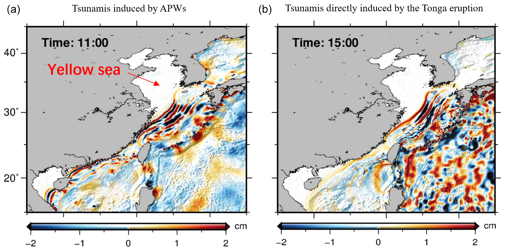
Figure 8Simulated tsunamis induced by the atmospheric-pressure waves (a) and tsunamis directly induced by the Tonga volcano eruption (b) near the coast of the Chinese mainland. The marked time represents the time after the volcanic eruption.
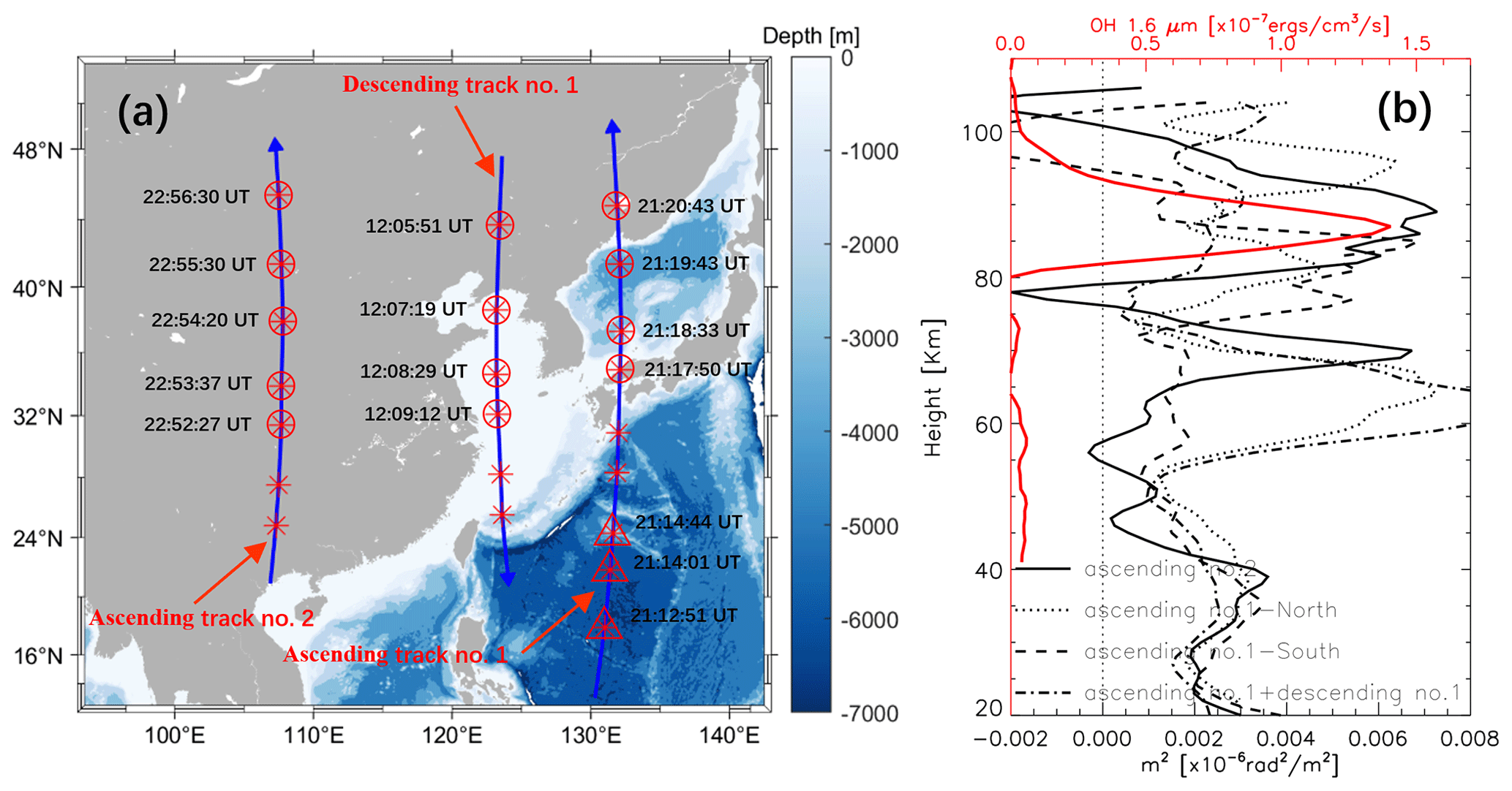
Figure 9(a) Ascending and descending SABER/TIMED satellite tracks over the Chinese mainland. The background is a representative ocean depth map. (b) Square of vertical wave number m2 profiles, with the solid black line profile derived from the ascending track no. 2 (marked by the red circle), the dotted line profile derived from the ascending track no. 1 north (marked by the red circle), the dashed line profile derived from the ascending track no. 1 south (marked by the red triangle), and the dashed–dotted line profile derived from the average of ascending track no. 1 and descending track no. 1 (marked by the red circle) from the SABER/TIMED measurement locations shown in panel (a). The red line represents the OH 1.6 µm emission intensity obtained by SABER/TIMED.
Figure 9a shows three TIMED satellite tracks with descending track no. 1 along the coast of China, ascending track no. 1 located east of the Korean Peninsula, and ascending track no. 2 located in inland China. Figure 9b shows the square of vertical wave number m2 profile (black) derived from the average temperature from the limb viewing of the sounding of the atmosphere using SABER/TIMED measurement locations marked by the red circles and triangles in Fig. 9a. We take the average temperature of ascending track no. 1; descending track no. 1 serves as the background temperature for wave packet no. 3, and ascending track no. 1 serves as the background temperature of wave packet nos. 4–5 when they propagate in the coastal vicinity. We take ascending track no. 2 as the background temperature of wave packet nos. 4–5 when they propagate in inland China. The peak height of the OH airglow layer is 87 km. We found that the propagation of wave packet no. 3 (dashed–dotted line) is in a state of free propagation in the coastal vicinity.
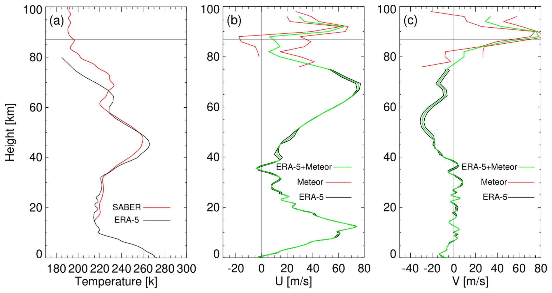
Figure 10The background field used for the ray-tracing analysis for the TIAPW event. (a) Saber temperature (red) comes from the average temperature of ascending track no. 1 and descending track no. 1 in Fig. 9, and the ERA5 temperature (black) comes from the average of 15:00 and 16:00 UT. (b) Meteor zonal wind field (red) and ERA5 zonal wind field (black). (c) Meteor meridional wind field (red) and ERA5 meridional wind field (black). The two red and black lines in panels (b) and (c) are, respectively, from 15:00 and 16:00 UT. The green lines represent the average of two lines. The meteor radar wind field is from Beijing station.
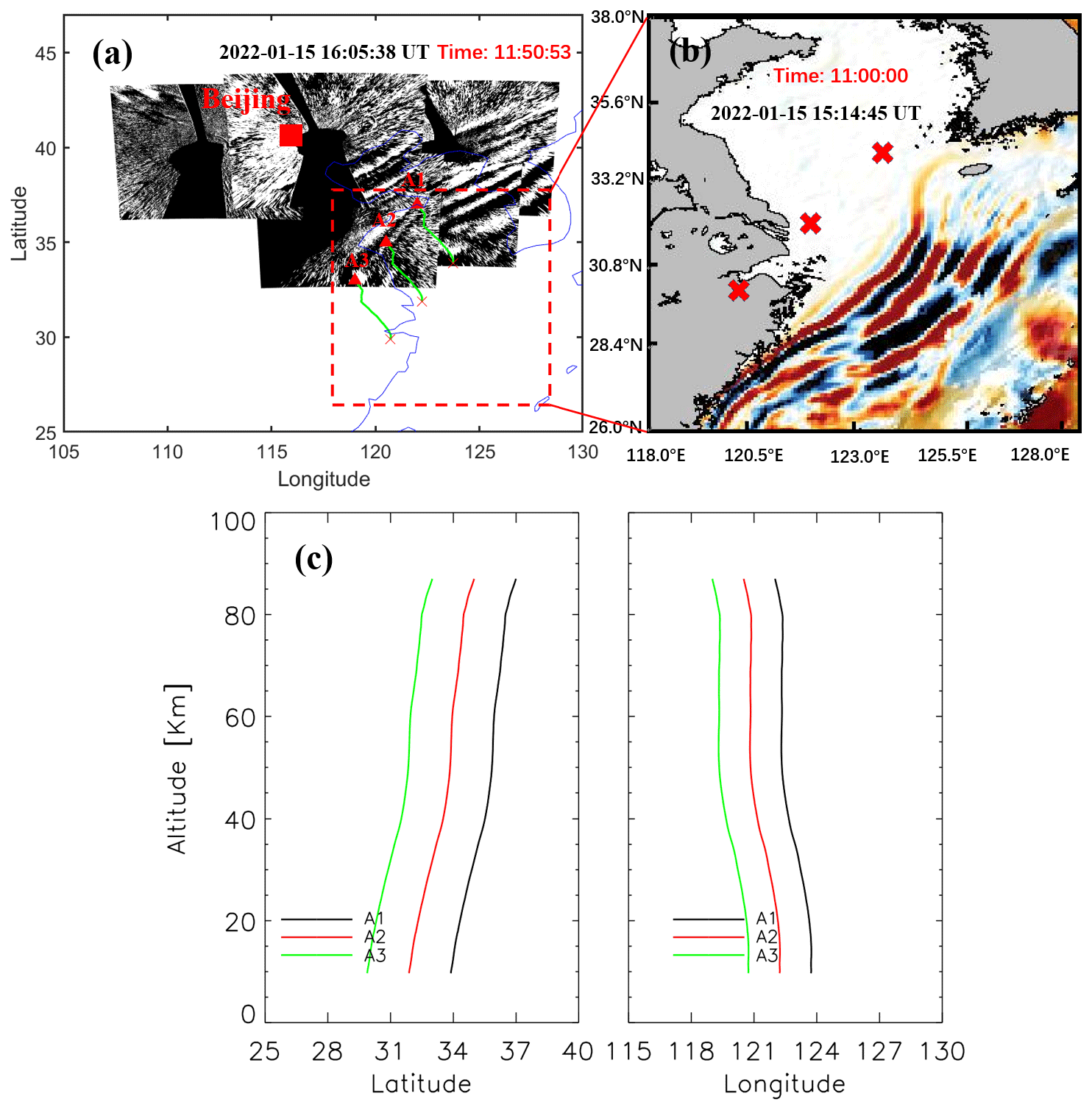
Figure 11(a) Backward ray-tracing results of wave packet no. 3 observed by the OH airglow network. The red triangles and red crosses represent the trace start and termination points, respectively. (b) Simulated tsunamis induced by the atmospheric-pressure wave (TIAPW) corresponding to the dotted rectangular area in panel (a). (c) Ray paths of the wave starting from the seven sampling points in panel (a).
Figure 10 shows the background field used for ray-tracing analysis for the TIAPW event. The temperature comes from TIMED/SABER and ERA5, and wind data comes from meteor radar and ERA5. Meteor radar wind field is from Beijing station (40.3° N, 116.2° E). Figure 11 shows the results of ray tracing for wave packet no. 3. We find that the source location of AGWs over the coast of the Chinese mainland falls near-coast where the tsunami occurred.
A tsunami simulation shows that the surface wave height along the coast of the Chinese mainland is of the order of 2 cm. There have been theoretical (Peltier and Hines, 1976) and observational (Grawe and Makela, 2015, 2017) studies on the relationship between the amplitude of tsunamis and GWs. Peltier and Hines (1976) found that a tsunami amplitude of ±1 cm at sea level can cause a vertical motion of the ionospheric E layer and F layer ±100 m. More direct observational evidence is that Grawe and Makela (2017) provided an airglow observation of tsunami-generated ionospheric signatures over Hawaii caused by the 16 September 2015 Illapel earthquake. They found that vertical disturbances on the sea surface not exceeding 2 cm (Fig. 3b in Grave and Makela, 2017) can create detectable signatures in the ionosphere (Fig. 1 in Grave and Makela, 2017). Therefore, we suggest that the waves with larger amplitudes following the leading of TIAPW interact with the atmosphere after arriving at the coast of the Chinese mainland to generate the upward-propagating AGW packet.
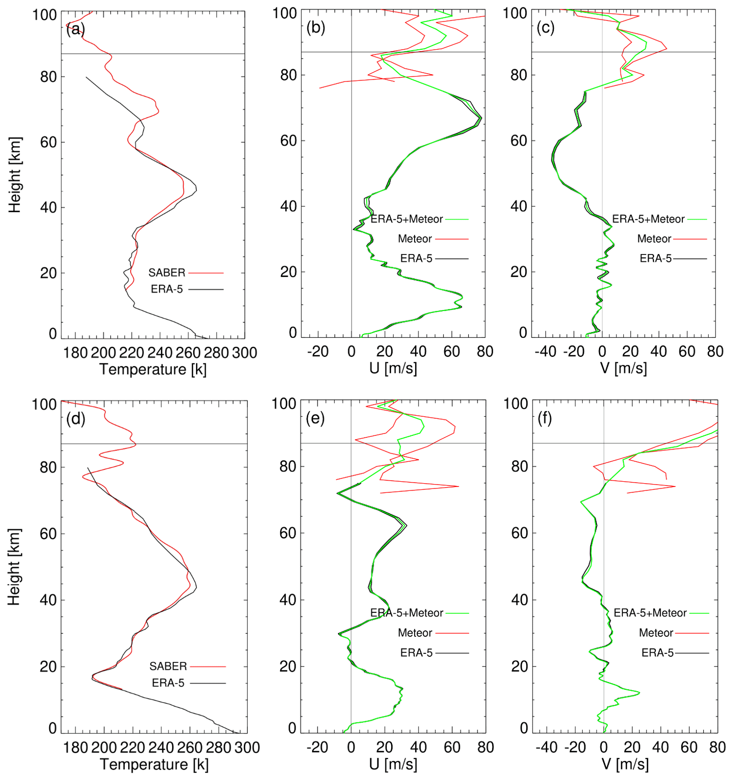
Figure 12Similar to Fig. 10 but for ray-tracing analysis for the TITVE events. The SABER temperature field in panel (a) comes from ascending track no. 1 (21:17:50, 21:18:33, 21:19:43, and 21:20:43 UT) in Fig. 9, and the meteor radar wind fields in panels (b) and (c) come from Beijing station. The SABER temperature field in panel (d) is from ascending track no. 1 (21:12:51, 21:14:01, and 21:14:44 UT) in Fig. 9, and the meteor radar wind fields in panels (e) and (f) are from Ledong station.
According to the theory of AGW dispersion, the AGW propagating obliquely has the following approximate relationship: ; φ is the oblique propagation angle, TB is the buoyancy period, and T is the intrinsic period. Azeem et al. (2017) found disturbances in the ionosphere excited by the 2011 Tohoku tsunamis when they reached the West Coast of the United States. They concluded that the fluctuations observed in TEC satisfy the AGW dispersion relation, and the period and horizontal wavelength of the TEC disturbances increased with distance from the West Coast of the USA.
From the airglow network observations, we found that wave packet nos. 4–5 excited by the tsunamis continue to propagate over the mainland more than 3000 km from the coast. If the AGWs observed by the airglow network propagate freely rather than being constrained by a duct, we will obtain the propagation characteristics similar to that observed by Azeem et al. (2017) in the ionosphere from TEC observations. TB is about 5 min from the SABER/TIMED observation. The period of wave packet no. 3 is between 5.5 and 8.5 min. The minimum propagation angle φ equals 35°, and the corresponding maximum propagation distance L is 125 km from estimation, where Hoh=87 km is the height of OH airglow layer. However, our observation does not satisfy the free oblique propagation dispersion theory of AGWs. In addition, we did not find that the GW horizontal wavelength increased with the distance from the shore, as predicted by the theory of AGW oblique propagation. Therefore, the AGWs excited by the tsunami we observed in the mesopause region may be modulated by a duct.
We did find a duct structure between 80 and 93 km (solid black line in Fig. 9b), while wave packet no. 3 was in a state of free propagation when it propagated around the coastal vicinity of the Chinese mainland (dotted line and dashed line). The duct almost includes the whole OH airglow layer. Therefore, we believe that AGWs generated by TITVE may enter the duct in the process of propagation over the Chinese mainland. The duct structure over the Chinese mainland can explain that the GWs generated by the tsunamis can propagate thousands of kilometers inland.
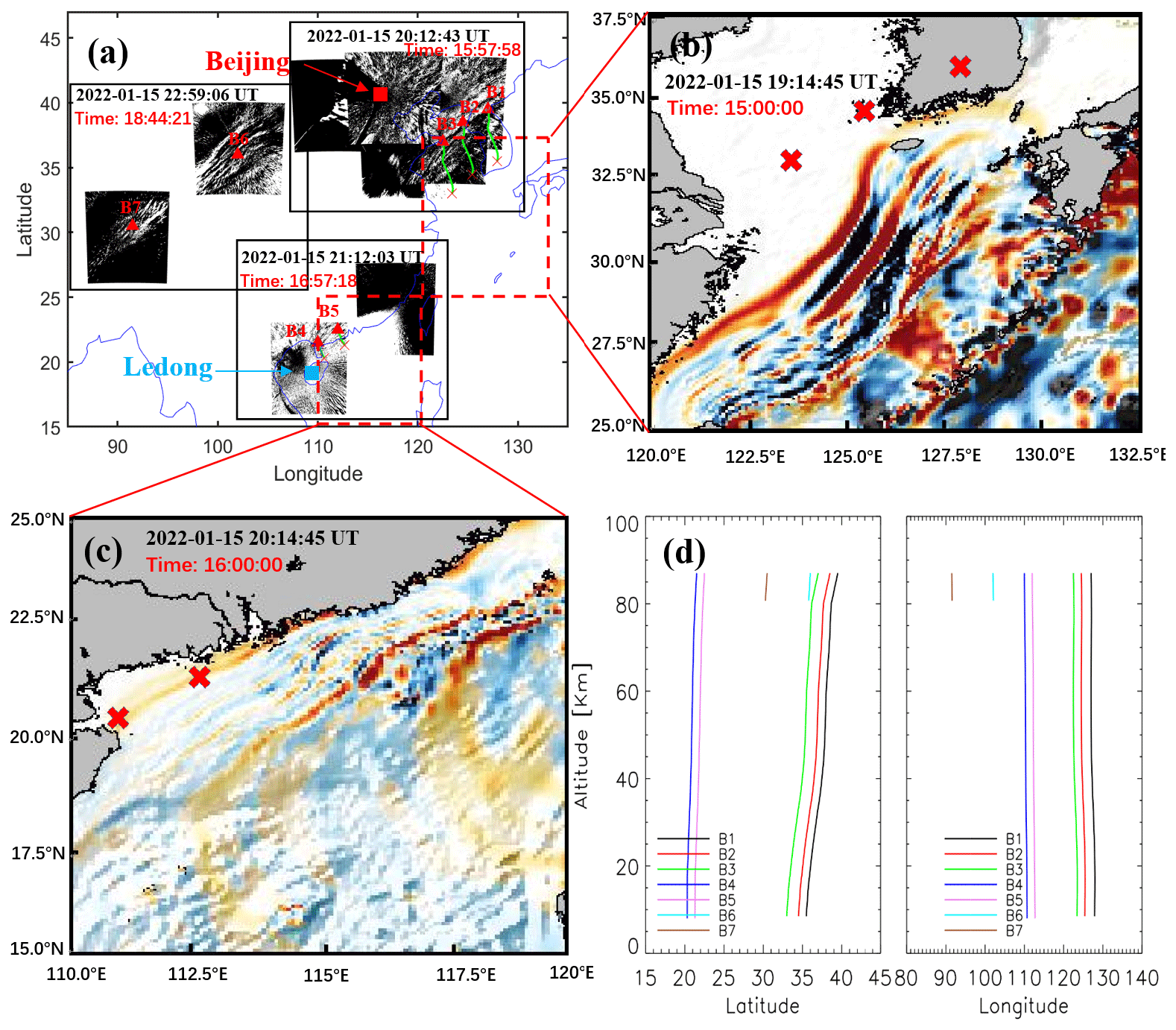
Figure 13(a) Backward ray-tracing results of the fourth and fifth groups of GWs observed by the OH airglow network. The red triangles and red crosses represent the trace start and termination points, respectively. Panels (b) and (c) show the simulated tsunami directly induced by the Tonga volcano eruption (TITVE), corresponding to the dotted rectangular area in panel (a). (c) Ray paths of the wave starting from the seven sampling points in panel (a).
Figure 13 shows the results of ray tracing for wave packet nos. 4–5. The background field used for ray-tracing analysis for wave packet nos. 4–5 is from Fig. 12. The meteor radar wind field is from Ledong station (18.3° N, 109.4° E). The horizontal wavelength of wave packet nos. 4 and 5 is observed near the coast by the OH airglow network at approximately 89 ± 6 km and 80 ± 4 km. We find that the source location of AGWs over the coast of the Chinese mainland falls in the near-tsunami area, while the location of AGW ray termination over the inland is around 80 km (positions B6 and B7 in Fig. 13d), which indicates that the wave meets the evanescent layer (Wrasse et al., 2006). This is consistent with the duct structure obtained through dispersion relation. Therefore, we suggest that TITVE interact with the atmosphere after arriving at the coast of the Chinese mainland to generate the upward-propagating AGW packet. After reaching the mesopause region, this wave packet enters the wave duct structure in the horizontal propagation process, and this wave duct supports wave packet no. 5 to propagate more than 3000 km inland China.
Strong atmospheric disturbances, including Lamb waves, acoustic waves, and GWs, were triggered by the 2022 HTHH volcano eruption. The HTHH submarine volcanic eruption also triggered an unusual tsunami, which can generate atmospheric gravity waves (Fig. 14). We observed five strong groups of atmospheric waves associated with the HTHH volcano eruption from the ground-based airglow network observations.
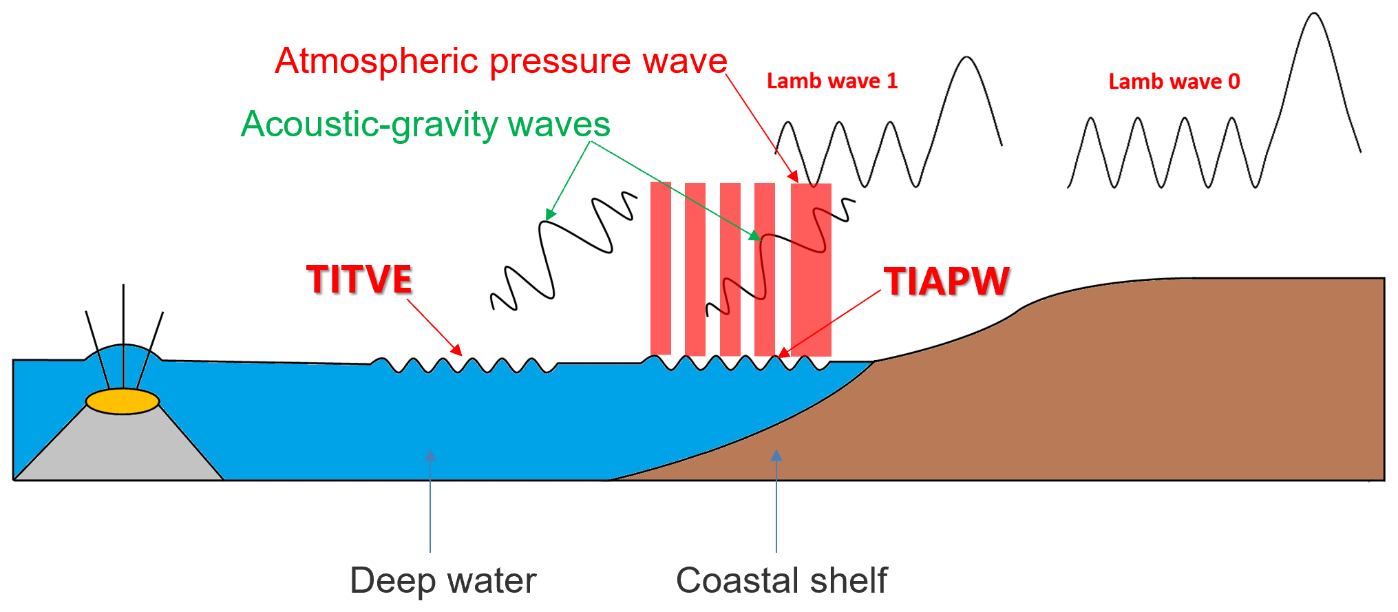
Figure 14The Tonga volcano eruptions triggered two types of tsunamis: one type of tsunami is induced by the atmospheric-pressure wave (TIAPW), and the other type tsunami is directly induced by the Tonga volcano eruption (TITVE). The acoustic gravity waves (AGWs) caused by tsunamis can propagate to the mesopause region.
The phase speed of the wave packet no. 1 leading front is approximately 309 m s−1, which is observed almost simultaneously with the surface Lamb wave L0 mode. The high-frequency wave trains following the wave packet no. 1 leading front observed by the northern OH airglow imager network may also be related to the dissipation of the leading waves. Wave packet no. 2, with an average phase speed of 236 m s−1, may be considered Lamb wave L1 mode, which exhibits internal GW behavior. Wave packet no. 3 and wave packet nos. 4–5 are generated by TIAPW and TITVE from backward ray-tracing analysis. The horizontal phase speed distribution range of wave packet nos. 3–5 is 200 to 215 m s−1, which is smaller than that of wave packet nos. 1–2. For amplitude, the average amplitude of the Lamb wave L1 mode (5.4 %) is higher than that of the Lamb wave L0 mode (3.2 %), while wave packet nos. 3, 4, and 5 have relatively small amplitudes, mainly distributed between 0.85 % and 1.25 %. The horizontal wavelengths of the atmospheric AGWs observed by the airglow network are very consistent with those of the tsunami near the coast. This is the first time that we observed the AGWs in the mesopause region triggered by the tsunamis using optical detection equipment. It is also the first time to report atmospheric gravity waves excited by TIAPW.
When the wave excited by TITVE propagates far away from the coast, the characteristics of AGWs are not consistent with the dispersion of free-propagation AGWs. We find these wave packets are controlled by the duct, which can support the propagation of these GWs for thousands of kilometers after the tsunami was stopped at the coast. Therefore, tsunamis can have a significant impact on the upper atmosphere over inland areas far from the ocean through AGWs.
The 2022 HTHH volcano eruption formed a complex coupling relationship in the land–ocean–atmosphere system (Fig. 14). First, the heat released by the eruption has a direct impact on the ocean, causing temperature changes in the surrounding waters. This can lead to changes in the marine environment, affecting the behavior, distribution, and ecosystem structure of organisms.
Meanwhile, volcanoes release gases such as carbon dioxide and sulfur dioxide. Carbon dioxide is one of the greenhouse gases that can cause an increase in the Earth's temperature, leading to global warming. Sulfur dioxide can cause sulfuric acid mist in the atmosphere, which affects the reflectivity and temperature of the atmosphere and thus affects the global climate.
Moreover, the 2022 HTHH volcano eruptions also trigger atmospheric waves and tsunamis. The surface atmospheric-pressure wave generated by the 2022 HTHH volcano eruption can affect the upper atmosphere. The conventional tsunami triggered by the Tonga volcano generated AGWs. The atmospheric-pressure wave from the eruption generated a fast tsunami never before observed by tsunami observation networks. When the tsunamis reach the coast, their speeds decrease but their amplitudes increase, and the AGWs generated by them will also affect the upper atmosphere. These AGWs play an important coupling role between the ocean and the atmosphere by affecting the density and pressure distribution of the atmosphere during propagation, leading to changes in the wind field and affecting global atmospheric circulation. This study exhibits special dynamic coupling process between the air and sea via acoustic gravity waves (Fig. 14). This indirect impact on the upper atmosphere provides a new perspective for us to study the coupling between the ocean and the atmosphere and a key opportunity to improve the air–sea coupling model, thereby enhancing our future ability to make tsunami warning forecasts.
The multi-layer airglow network data are available at https://data2.meridianproject.ac.cn/data (MPDC, 2024). TIMED/SABER data are accessible from http://saber.gats-inc.com/data.php (Mlynczak et al., 2023). The ERA5 reanalysis data are available for downloaded from the Copernicus Climate Change Service Climate Data Store at https://doi.org/10.24381/cds.bd0915c6 (Hersbach et al., 2023). Himawari-8 data are distributed by the Center for Environmental Remote Sensing (http://www.cr.chiba-u.jp/databases/GEO/H8_9/FD/index_en_V20190123.html, Higuchi et al., 2024; Otsuka, 2022). Meteor radar data were provided by the Beijing National Observatory of Space Environment, Institute of Geology and Geophysics, Chinese Academy of Sciences, through the geophysics center, the National Earth System Science Data Center (http://wdc.geophys.ac.cn, NESCDC, 2024).
A multi-group of strong atmospheric waves observed over China associated with the 2022 Hunga Tonga–Hunga Ha′apai volcano eruptions is available for view (https://doi.org/10.5446/66190, Li, 2024c). An animation series of OH airglow disturbances associated with the 2022 Hunga Tonga–Hunga Ha′apai volcano eruptions is available for view (https://doi.org/10.5446/s_1689, Li, 2024b). A strong wave front observed by an OI 630 nm airglow imager over China associated with the 2022 Hunga Tonga–Hunga Ha′apai volcano eruptions is available for view (https://doi.org/10.5446/66280, Li, 2024a).
JX and QL conceived the idea of the article. QL carried out the data analysis, interpretation, and manuscript preparation. ARG developed and performed the numerical simulations. WL and YZ compiled, processed, and analyzed satellite data. HL, XL, and WY contributed to the data interpretation and manuscript preparation. All authors discussed the results and commented on the paper.
The contact author has declared that none of the authors has any competing interests.
Publisher's note: Copernicus Publications remains neutral with regard to jurisdictional claims made in the text, published maps, institutional affiliations, or any other geographical representation in this paper. While Copernicus Publications makes every effort to include appropriate place names, the final responsibility lies with the authors.
We thank the National Science Foundation of China (grant nos. 42374205 and 41974179). We acknowledge the use of data from the Chinese Meridian Project. We appreciate the TIMED/SABER team for providing the temperature and emission intensity data and the National Earth System Science Data Center for providing the meteor radar data. We also thank the European Centre for Medium-Range Weather Forecasts (ECMWF) for the provision of the ERA5 data and the Center for Environmental Remote Sensing (CERS) for the Himawari-8 data.
This research has been supported by the National Natural Science Foundation of China (grant nos. 42374205, and 41974179) and the Specialized Research Fund of National Space Science Center, Chinese Academy of Sciences (grant no. E4PD3010). The project has also been supported by the Specialized Research Fund for State Key Laboratories. Aditya Riadi Gusman has been supported by the Aotearoa / New Zealand Ministry for Business, Innovation, and Employment (MBIE) through the Rapid Characterisation of Earthquakes and Tsunami (R-CET): Fewer deaths and faster recovery project (Endeavour fund).
This paper was edited by John Plane and reviewed by two anonymous referees.
Adam, D.: Tonga volcano eruption created puzzling ripples in Earth's atmosphere, Nature, 601, 497, https://doi.org/10.1038/d41586-022-00127-1, 2022.
Amores, A., Monserrat, S., Marcos, M., Argüeso, D., Villalonga, J., Jordà, G., and Gomis, D.: Numerical simulation of atmospheric Lamb waves generated by the 2022 Hunga-Tonga volcanic eruption, Geophys. Res. Lett., 49, e2022GL098240, https://doi.org/10.1029/2022GL098240, 2022.
Astafyeva, E., Maletckii, B., Mikesell, T. D., Munaibari, E., Ravanelli, M., Coisson, P., Manta, F., and Rolland, L.: The 15 January 2022 Hunga Tonga eruption history as inferred from ionospheric observations, Geophys. Res. Lett., 49, e2022GL098827, https://doi.org/10.1029/2022GL098827, 2022.
Azeem, I., Vadas, S. L., Crowley, G., and Makela, J. J.: Traveling ionospheric disturbances over the United States induced by gravity waves from the 2011 Tohoku tsunami and comparison with gravity wave dissipative theory, J. Geophys. Res.-Space, 122, 3430–3447, https://doi.org/10.1002/2016JA023659, 2017.
Becker, E. and Vadas, S. L.: Secondary gravity waves in the winter mesosphere: Results from a high-resolution global circulation model, J. Geophys. Res.-Atmos., 123, 2605–2627, https://doi.org/10.1002/2017JD027460, 2018.
Beer, T.: Atmospheric Waves, John Wiley, New York, 300 pp., ISBN 0470061855, 1974.
Carvajal, M., Sepúlveda, I., Gubler, A., and Garreaud, R.: Worldwide signature of the 2022 Tonga volcanic tsunami, Geophys. Res. Lett., 49, e2022GL098153, https://doi.org/10.1029/2022GL098153, 2022.
Donn, W. L. and Balachandran, N. K.: Mount St. Helens eruption of 18 May 1980: Air waves and explosive yield, Science, 213, 539–541, https://doi.org/10.1126/science.213.4507.539, 1981.
Duncombe, J.: The surprising reach of Tonga's Giant atmospheric waves, Eos T. Am. Geophys. Un., 103, https://doi.org/10.1029/2022EO220050, 2022.
Francis, S. H.: Acoustic-gravity modes and large-scale traveling ionospheric disturbances of a realistic, dissipative atmosphere, J. Geophys. Res., 78, 2278–2301, https://doi.org/10.1029/JA078i013p02278, 1973.
Garcia, F. J., Taylor, M. J., and Kelley, M. C.: Two-dimensional spectral analysis of mesospheric airglow image data, Appl. Optics, 36, 7374–7385, https://doi.org/10.1364/AO.36.007374, 1997.
Ghent, J. N. and Crowell, B. W.: Spectral characteristics of ionospheric disturbances over the southwestern Pacific from the 15 January 2022 Tonga eruption and tsunami, Geophys. Res. Lett., 49, e2022GL100145, https://doi.org/10.1029/2022GL100145, 2022.
Gossard, E. E. and Hooke, W. H.: Waves in the Atmosphere, Elsevier, Amsterdam, the Netherlands, 456 pp., 1975.
Grawe, M. A. and Makela, J. J.: The ionospheric responses to the 2011 Tohoku, 2012 Haida Gwaii, and 2010 Chile tsunamis: Effects of tsunami orientation and observation geometry, Earth and Space Science, 2, 472–483, https://doi.org/10.1002/2015EA000132, 2015.
Grawe, M. A. and Makela, J. J.: Observation of tsunami-generated ionospheric signatures over Hawaii caused by the 16 September 2015 Illapel earthquake, J. Geophys. Res.-Space, 122, 1128–1136, https://doi.org/10.1002/2016JA023228, 2017.
Gusman, A. R., Roger, J., Noble, C., Wang, X., Power, W., and Burbidge, D.: The 2022 Hunga Tonga-Hunga Ha′apai Volcano Air-Wave Generated Tsunami, Pure Appl. Geophys., 179, 3511–3525, https://doi.org/10.1007/s00024-022-03154-1, 2022.
Harkrider, D. and Press, F.: The Krakatoa air-sea waves: An example of pulse propagation in coupled systems, Geophys. J. Roy. Astr. S. 13, 149–159, https://doi.org/10.1111/j.1365-246X.1967.tb02150.x, 1967.
Hersbach, H., Bell, B., Berrisford, P., Hirahara, S., Horányi, A., Muñoz-Sabater, J., Nicolas, J., Peubey, C., Radu, R., Schepers, D., Simmons, A., Soci, C., Abdalla, S., Abellan, X., Balsamo, G., Bechtold, P., Biavati, G., Bidlot, J., Bonavita, M., De Chiara, G., Dahlgren, P., Dee, D., Diamantakis, M., Dragani, R., Flemming, J., Forbes, R., Fuentes, M., Geer, A., Haimberger, L., Healy, S., Hogan, R. J., Hólm, E., Janisková, M., Keeley, S., Laloyaux, P., Lopez, P., Lupu, C., Radnoti, G., deRosnay, P., Rozum, I., Vamborg, F., Villaume, S., and Thépaut, J. N.: The ERA5 global reanalysis, Q. J. Roy. Meteor. Soc., 146, 1999–2049, https://doi.org/10.1002/qj.3803, 2020.
Hersbach, H., Bell, B., Berrisford, P., Biavati, G., Horányi, A., Muñoz Sabater, J., Nicolas, J., Peubey, C., Radu, R., Rozum, I., Schepers, D., Simmons, A., Soci, C., Dee, D., and Thépaut, J.-N.: ERA5 hourly data on pressure levels from 1940 to present, Copernicus Climate Change Service (C3S) Climate Data Store (CDS) [data set], https://doi.org/10.24381/cds.bd0915c6, 2023.
Hickey, M. P., Schubert, G., and Walterscheid, R. L.: Propagation of tsunami-driven gravity waves into the thermosphere and ionosphere, J. Geophys. Res., 114, A08304, https://doi.org/10.1029/2009JA014105, 2009.
Hickey, M. P., Schubert, G., and Walterscheid, R. L.: Atmospheric airglow fluctuations due to a tsunami-driven gravity wave disturbance, J. Geophys. Res., 115, A06308, https://doi.org/10.1029/2009JA014977, 2010.
Higuchi, A., Takenaka, H., and Toyoshima, K.: HIMAWARI 8/9 gridded full-disk (FD) data Version 02 (V20190123), Center for Environmental Remote Sensing (CEReS), Chiba University, Japan [data set], http://www.cr.chiba-u.jp/databases/GEO/H8_9/FD/index_en_V20190123.html, last access: 20 January 2024.
Hines, C.: Gravity waves in the atmosphere, Nature, 239, 73–78, https://doi.org/10.1038/239073A0, 1972.
Inchin, P. A., Heale, C. J., Snively, J. B., and Zettergren, M. D.: The dynamics of nonlinear atmospheric acoustic-gravity waves generated by tsunamis over realistic bathymetry, J. Geophys. Res.-Space, 125, e2020JA028309, https://doi.org/10.1029/2020JA028309, 2020.
Inchin, P. A., Heale, C. J., Snively, J. B., and Zettergren, M. D.: Numerical modeling of tsunami-generated acoustic-gravity waves in mesopause airglow, J. Geophys. Res.-Space, 127, e2022JA030301, https://doi.org/10.1029/2022JA030301, 2022.
Koketsu K. and Higashi S.: Three-dimensional topography of the sediment/basement interface in the Tokyo Metropolitan area, Central Japan, B. Seismol. Soc. Am., 82, 2328–2349, https://doi.org/10.1785/BSSA0820062328, 1992.
Kubota, T., Saito, T., and Nishida, K.: Global fast-traveling tsunamis driven by atmospheric Lamb waves on the 2022 Tonga eruption, Science, 377, 91–94, https://doi.org/10.1126/science.abo4364, 2022.
Laughman, B., Fritts, D. C., and Lund, T. S.: Tsunami-driven gravity waves in the presence of vertically varying background and tidal wind structures, J. Geophys. Res.-Atmos., 122, 5076–5096, https://doi.org/10.1002/2016JD025673, 2017.
Li, Q.: A strong wave front observed by an OI 630 nm airglow imager over China associated with the 2022 Hunga Tonga–Hunga Ha′apai volcano eruptions, TIB AV-Portal [video], https://doi.org/10.5446/66280, 2024a.
Li, Q.: Animation series of OH airglow disturbances associated with the 2022 Hunga Tonga–Hunga Ha′apai volcano eruptions, TIB AV-Portal [video], https://doi.org/10.5446/s_1689, 2024b.
Li, Q.: Multi-group of strong atmospheric waves observed over China associated with the 2022 Hunga Tonga–Hunga Ha′apai volcano eruptions, TIB AV-Portal [video], https://doi.org/10.5446/66190, 2024c.
Li, Q., Xu, J., Liu, H., Liu, X., and Yuan, W.: How do gravity waves triggered by a typhoon propagate from the troposphere to the upper atmosphere?, Atmos. Chem. Phys., 22, 12077–12091, https://doi.org/10.5194/acp-22-12077-2022, 2022.
Li, X., Ding, F., Yue, X., Mao, T., Xiong, B., and Song, Q.: Multiwave structure of traveling ionospheric disturbances excited by the Tonga volcanic eruptions observed by a dense GNSS network in China, Space Weather, 21, e2022SW003210, https://doi.org/10.1029/2022SW003210, 2023.
Lighthill, M. J.: Waves in Fluids, Cambridge University Press, Cambridge, UK, New York, 504 pp., ISBN 0-521-01045-4, 1978.
Lin, J.-T., Rajesh, P. K., Lin, C. C. H., Chou, M.-Y., Liu, J.-Y., Yue, J., Hsiao,T., Tsai, H., Chao, H., and Kung, M.: Rapid conjugate appearance of the giant ionospheric Lamb wave signatures in the northern hemisphere after Hunga-Tonga volcano eruptions, Geophys. Res. Lett., 49, e2022GL098222, https://doi.org/10.1029/2022GL098222, 2022.
Lindzen, R. S. and Blake, D.: Lamb waves in the presence of realistic distributions of temperature and dissipation, J. Geophys. Res., 77, 2166–2176, https://doi.org/10.1029/JC077i012p02166, 1972.
Liu, H.-L., Wang, W., Huba, J. D., Lauritzen, P. H., and Vitt, F.: Atmospheric and Ionospheric Responses to Hunga-Tonga Volcano Eruption Simulated by WACCM-X, Geophys. Res. Lett., 50, e2023GL103682, https://doi.org/10.1029/2023GL103682, 2023.
Liu, X., Xu, J., Yue, J., and Kogure, M.: Strong gravity waves associated with Tonga volcano eruption revealed by SABER observations, Geophys. Res. Lett., 49, e2022GL098339, https://doi.org/10.1029/2022GL098339, 2022.
Makela, J. J., Lognonné, P., Hébert, H., Gehrels, T., Rolland, L., Allgeyer, S., Kherani, A., Occhipinti, G., Astafyeva, E., Coïsson, P., Loevenbruck, A., Clévédé, E., Kelley, M. C., and Lamouroux, J.: Imaging and modeling the ionospheric airglow response over Hawaii to the tsunami generated by the Tohoku earthquake of 11 March 2011, Geophys. Res. Lett., 38, e2011GL047860, https://doi.org/10.1029/2011GL047860, 2011.
Mlynczak, M. G., Marshall, B. T., Garcia, R. R., Hunt, L., Yue, J., Harvey, V. L., Lopez-Puertas, M., Mertens, C., and Russell, J.: Algorithm stability and the long-term geospace data record from TIMED/SABER, Geophys. Res. Lett., 50, 1–7, https://doi.org/10.1029/2022GL102398, 2023 (data available at http://saber.gats-inc.com/data.php, last access: 10 January 2024).
MPDC: Airglow data, MPDC [data set], https://data2.meridianproject.ac.cn/data, last access: 15 January 2024.
NESCDC: Meteor data, NESCDC [data set], http://wdc.geophys.ac.cn, last access: 15 January 2024.
Nishikawa, Y., Yamamoto, My., Nakajima, K., Hamama, I., Saito, H., Kakinami, Y., Yamada, M., and Ho, T.: Observation and simulation of atmospheric gravity waves exciting subsequent tsunami along the coastline of Japan after Tonga explosion event, Sci. Rep.-UK, 12, 22354, https://doi.org/10.1038/s41598-022-25854-3, 2022.
Occhipinti, G., Rolland, L., Lognonné, P., and Watada, S.: From Sumatra 2004 to Tohoku-Oki 2011: The systematic GPS detection of the ionospheric signature induced by tsunamigenic earthquakes, J. Geophys. Res.-Space, 118, 3626–3636, https://doi.org/10.1002/jgra.50322, 2013.
Omira, R., Ramalho, R. S., Kim, J., González, P. J., Kadri, U., Miranda,J. M., Carrilho, F., and Baptista,M. A.: Global Tonga tsunami explained by a fast-moving atmospheric source, Nature, 609, 734–740, https://doi.org/10.1038/s41586-022-04926-4, 2022.
Otsuka, S.: Visualizing Lamb waves from a volcanic eruption using meteorological satellite Himawari-8, Geophys. Res. Lett., 49, https://doi.org/10.1029/2022GL098324, 2022 (data available at http://www.cr.chiba-u.jp/databases/GEO/H8_9/FD/index_en_V20190123.html, last access: 20 January 2024).
Peltier, W. and Hines, C.: On the possible detection of tsunamis by a monitoring of the ionosphere, J. Geophys. Res., 81, 1995–2000, https://doi.org/10.1029/JC081i012p01995, 1976.
Poblet, F. L., Chau, J. L., Conte, J. F., Vierinen, J., Suclupe, J., Liu, A., and Rodriguez, R. R.: Extreme horizontal wind perturbations in the mesosphere and lower thermosphere over South America associated with the 2022 Hunga eruption, Geophys. Res. Lett., 50, e2023GL103809, https://doi.org/10.1029/2023GL103809, 2023.
Pradipta, R., Carter, B. A., Currie, J. L., Choy, S., Wilkinson, P., Maher, P., and Marshall, R.: On the propagation of traveling ionospheric disturbances from the Hunga Tonga-Hunga Ha′apai volcano eruption and their possible connection with tsunami waves, Geophys. Res. Lett., 50, e2022GL101925, https://doi.org/10.1029/2022GL101925, 2023.
Press, F. and Harkrider, D. G.: Propagation of acoustic-gravity waves in the atmosphere, J. Geophys. Res., 67, 3889–3908, https://doi.org/10.1029/JZ067i010p03889, 1962.
Salmon, R.: Introduction to ocean waves, Scripps Inst. of Oceanogr., Univ. of Calif., San Diego, USA, 2014.
Sepúlveda, I., Carvajal, M., and Agnew, D. C.: Global winds shape planetary-scale Lamb waves, Geophys. Res. Lett., 50, e2023GL106097, https://doi.org/10.1029/2023GL106097, 2023.
Smith, S. M., Martinis, C. R., Baumgardner, J., and Mendillo, M.: All-sky imaging of transglobal thermospheric gravity waves generated by the March 2011 Tohoku Earthquake, J. Geophys. Res.-Space, 120, 10992–10999, https://doi.org/10.1002/2015JA021638, 2015.
Stober, G., Liu, A., Kozlovsky, A., Qiao, Z., Krochin, W., Shi, G., Kero, J., Tsutsumi, M., Gulbrandsen, N., Nozawa, S., Lester, M., Baumgarten, K., Belova, E., and Mitchell, N.: Identifying gravity waves launched by the Hunga Tonga–Hunga Ha′apai volcanic eruption in mesosphere/lower-thermosphere winds derived from CONDOR and the Nordic Meteor Radar Cluster, Ann. Geophys., 41, 197–208, https://doi.org/10.5194/angeo-41-197-2023, 2023.
Stober, G., Vadas, S. L., Becker, E., Liu, A., Kozlovsky, A., Janches, D., Qiao, Z., Krochin, W., Shi, G., Yi, W., Zeng, J., Brown, P., Vida, D., Hindley, N., Jacobi, C., Murphy, D., Buriti, R., Andrioli, V., Batista, P., Marino, J., Palo, S., Thorsen, D., Tsutsumi, M., Gulbrandsen, N., Nozawa, S., Lester, M., Baumgarten, K., Kero, J., Belova, E., Mitchell, N., Moffat-Griffin, T., and Li, N.: Gravity waves generated by the Hunga Tonga–Hunga Ha′apai volcanic eruption and their global propagation in the mesosphere/lower thermosphere observed by meteor radars and modeled with the High-Altitude general Mechanistic Circulation Model, Atmos. Chem. Phys., 24, 4851–4873, https://doi.org/10.5194/acp-24-4851-2024, 2024.
Swenson, G. R. and Mende, S. B.: OH emission and gravity waves (including a breaking wave) in all-sky imagery from Bear Lake, UT, Geophys. Res. Lett., 21, 2239–2242, https://doi.org/10.1029/94GL02112, 1994.
Symons, G. J.: The Eruption of Krakatoa, and Subsequent Phenomena, Trubner & Co., London, ISBN 978-0343922986, 1888.
Takahashi, H., Figueiredo, C. A. O. B., Barros, D., Wrasse, C. M., Giongo, G. A., Honda, R. H., Vital, L. F. R., Resende, L. C. A., Nyassor, P. K., Ayorinde, T. T., Carmo, C. S., Padua, M. B., and Otsuka, Y.: Ionospheric disturbances over South America related to Tonga volcanic eruption, Earth Planets Space, 75, 92, https://doi.org/10.1186/s40623-023-01844-1, 2023.
Tang, J., Kamalabadi, F., Franke, S. J., Liu, A. Z., and Swenson, G. R.: Estimation of gravity wave momentum flux with spectroscopic imaging, IEEE T. Geosci. Remote, 43, 103–109, https://doi.org/10.1109/TGRS.2004.836268, 2005.
Themens, D. R., Watson, C., Zagar, N., Vasylkevych, S., Elvidge, S., McCaffrey, A., Prikryl, P., Reid, B., Wood, A., and Jayachandran, P. T.: Global propagation of ionospheric disturbances associated with the 2022 Tonga volcanic eruption, Geophys. Res. Lett., 49, e2022GL098158, https://doi.org/10.1029/2022GL098158, 2022.
Vadas, S. L. and Becker, E.: Numerical modeling of the excitation, propagation, and dissipation of primary and secondary gravity waves during wintertime at McMurdo Station in the Antarctic, J. Geophys. Res.-Atmos., 123, 9326–9369, https://doi.org/10.1029/2017JD027974, 2018.
Vadas, S. L., Makela, J. J., Nicolls, M. J., and Milliff, R. F.: Excitation of gravity waves by ocean surface wave packets: Upward propagation and reconstruction of the thermospheric gravity wave field, J. Geophys. Res.-Space, 120, 9748–9780, https://doi.org/10.1002/2015JA021430, 2015.
Vadas, S. L., Zhao, J., Chu, X., and Becker, E.: The excitation of secondary gravity waves from local body forces: Theory and observation, J. Geophys. Res.-Atmos., 123, 9296–9325, https://doi.org/10.1029/2017JD027970, 2018.
Vadas, S. L., Becker, E., Figueiredo, C., Bossert, K., Harding, B. J., and Gasque, L. C.: Primary and secondary gravity waves and large-scale wind changes generated by the Tonga volcanic eruption on 15 January 2022: Modeling and comparison with ICON-MIGHTI winds, J. Geophys. Res.-Space, 128, e2022JA031138, https://doi.org/10.1029/2022JA031138, 2023.
Xu, J., Li, Q., Yue, J., Hoffmann, L., Straka, W. C., Wang, C., Liu, M., Yuan, W., Han, S., Miller, S. D., Sun, L., Liu, X., Liu, W., Yang, J., and Ning, B.: Concentric gravity waves over northern China observed by an airglow imager network and satellites, J. Geophys. Res.-Atmos., 120, 11058–11078, https://doi.org/10.1002/2015JD023786, 2015.
Xu, J., Li, Q., Sun, L., Liu, X., Yuan, W., Wang, W., Yue, J., Zhang, S., Liu, W., Jiang, G., Wu, K., Gao, H., and Lai, C.: The Ground-Based Airglow Imager Network in China: Recent Observational Results, Geophys. Monogr. Ser., 261, 365–394, https://doi.org/10.1002/9781119815631.ch19, 2021.
Yamada, M., Ho, T.-C., Mori, J., Nishikawa, Y., and Yamamoto, M.-Y.: Tsunami triggered by the Lamb wave from the 2022 Tonga volcanic eruption and transition in the offshore Japan region, Geophys. Res. Lett., 49, e2022GL098752, https://doi.org/10.1029/2022GL098752, 2022.
Yeh, K. C. and Liu, C. H.: Acoustic-Gravity Waves in the Upper Atmosphere, Rev. Geophys. Space Ge., 12, 193, https://doi.org/10.1029/RG012i002p00193, 1974.
Wrasse, C. M., Nakamura, T., Tsuda, T., Takahashi, H., Medeiros, A. F., Taylor, M. J., Gobbi, D., Salatun, A., Suratno, E. A., and Admiranto, A. G.: Reverse ray tracing of the mesospheric gravity waves observed at 23° S (Brazil) and 7° S (Indonesia) in airglow imagers, J. Atmos. Sol.-Terr. Phy., 68, 163–181, https://doi.org/10.1016/j.jastp.2005.10.012, 2006.
Wright, C. J., Hindley, N. P., Alexander, M. J., Barlow, M., Hoffmann, L., Mitchell, C. N., Prata, F., Bouillon,M.and Carstens, J., Clerbaux, C., Osprey, S. M., Powell, N., Randall, C. E., and Yue, J.: Surface-to-space atmospheric waves from Hunga Tonga-Hunga Ha′apai eruption, Nature, 609, 741–746, https://doi.org/10.1038/s41586-022-05012-5, 2022.
Zhang, S., Vierinen, J., Aa, E., Goncharenko, L. P., Erickson, P., Rideout, W., Coster, A. J., and Spicher, A.: 2022 Tonga volcanic eruption induced global propagation of ionospheric disturbances via Lamb waves, Frontiers in Astronomy and Space Sciences, 9, 1–10, https://doi.org/10.3389/fspas.2022.871275, 2022.