Climatology of the terms and variables of transformed Eulerian-mean (TEM) equations from multiple reanalyses: MERRA-2, JRA-55, ERA-Interim, and CFSR

A 30-year (1980–2010) climatology of the major variables and terms of the transformed Eulerian-mean (TEM) momentum and thermodynamic equations is constructed by using four global atmospheric reanalyses: the Modern-Era Retrospective analysis for Research and Applications, Version 2 (MERRA-2); the Japanese 55-year Reanalysis (JRA-55); the European Centre for Medium-Range Weather Forecasts (ECMWF) interim reanalysis (ERA-Interim); and the Climate Forecast System Reanalysis (CFSR). Both the reanalysis ensemble mean (REM) and the differences in each reanalysis from the REM are investigated in the latitude–pressure domain for December–January–February and for June–July–August. For the REM investigation, two residual vertical velocities (the original one and one evaluated from residual meridional velocity) and two mass streamfunctions (from meridional and vertical velocities) are compared. Longwave (LW) radiative heating and shortwave (SW) radiative heating are also shown and discussed. For the TEM equations, the residual terms are also calculated and investigated for their potential usefulness, as the residual term for the momentum equation should include the effects of parameterized processes such as gravity waves, while that for the thermodynamic equation should indicate the analysis increment. Inter-reanalysis differences are investigated for the mass streamfunction, LW and SW heating, the two major terms of the TEM momentum equation (the Coriolis term and the Eliassen–Palm flux divergence term), and the two major terms of the TEM thermodynamic equation (the vertical temperature advection term and the total diabatic heating term). The spread among reanalysis TEM momentum balance terms is around 10 % in Northern Hemisphere winter and up to 50 % in Southern Hemisphere winter. The largest uncertainties in the thermodynamic equation (about 50 %) are found in the vertical advection, for which the structure is inconsistent with the differences in heating. The results shown in this paper provide basic information on the degree of agreement among recent reanalyses in the stratosphere and upper troposphere in the TEM framework.

1 Introduction

The transformed Eulerian-mean (TEM) set of equations (Andrews et al., 1987; see also Sect. 2.2 below) is a zonally averaged set of equations of atmospheric motion that describes the zonal mean characteristics of the atmospheric circulation. The response of the zonal mean flow to eddy momentum and heat fluxes is explicitly shown through the so-called Eliassen–Palm (EP) flux divergence term. The residual mean meridional circulation (${\stackrel{\mathrm{‾}}{v}}^{*}$, ${\stackrel{\mathrm{‾}}{\mathit{\omega }}}^{*}$ or ${\stackrel{\mathrm{‾}}{w}}^{*}$) that appears in the TEM equations is known to be a very good approximation of the global mass circulation, also known as the Brewer–Dobson (BD) circulation (Butchart, 2014).

Studies investigating the residual mean meridional circulation, EP flux, and other TEM variables and terms in the real atmosphere typically use global meteorological analysis data, or more specifically global atmospheric reanalysis data (e.g. SPARC, 2022, and the references therein), as these variables and terms are not directly observable. However, there are different versions of reanalyses from different reanalysis-producing centres, and different reanalyses may show substantially different results for the same diagnostics due to different methodological details of the reanalysis systems (SPARC, 2022). SPARC (2022) provided comparisons of some key TEM variables and terms among different reanalyses at climatological or seasonal timescales: tropical upwelling at 70 hPa and EP flux divergence for the 100–70 and 50–3 hPa regions (in its Chapter 5), the residual mean meridional circulation (${\stackrel{\mathrm{‾}}{v}}^{*}$, ${\stackrel{\mathrm{‾}}{w}}^{*}$) as well as temperature and zonal wind up to the 0.1 hPa level (Chapter 11; see also Chapter 3 for a more detailed analysis for temperature and horizontal winds up to 1 hPa), and others. Diabatic heating in the tropical upper troposphere and lower stratosphere was evaluated in Chapters 5 and 8 and ozone data products in the whole stratosphere in Chapter 4.

We note that reanalysis systems are complex and it is difficult to attribute particular differences among the reanalysis data products to particular components of the system. The reanalysis system consists of a forecast model, assimilation scheme, and assimilated observational data. Different reanalyses use different models with different choices of e.g. particular sub-grid-scale parameterizations (see Chapter 2 of SPARC, 2022, for a concise summary of these). The final reanalysis data products are largely determined not by particular choices in the forecast models but rather by the observational data assimilation, i.e. which observational data are assimilated and how they are assimilated, including particular parameter settings in the assimilation scheme. Although differences or issues among reanalyses can only be attributed to particular components through parameter perturbation experiments conducted by the data providers, reanalysis data users can and should identify and highlight issues so that they are more likely to be attributed and addressed in future reanalysis products.

In this paper, we evaluate all major variables and terms of the TEM momentum and thermodynamic equations from four reanalysis datasets at climatological timescales, focusing on their latitude–pressure distributions in the December–January–February (DJF) and June–July–August (JJA) seasons. The analysis periods extend from December 1980 to February 2010 for DJF and from 1981 to 2010 for JJA. Results for the two equinoctial seasons, March–April–May (MAM) and September–October–November (SON), both for 1981–2010, are provided in the Supplement. Distributions of longwave (LW) and shortwave (SW) radiative heating in DJF and JJA are also investigated. The monthly imbalance in the TEM momentum equation is also provided as a residual term that results mainly from sub-grid-scale processes such as (parameterized) gravity wave drag (Sato and Hirano, 2019). The monthly imbalance of the TEM thermodynamic equation is expressed as a residual term that results mainly from the so-called analysis increment, which represents the average difference between the analysis state and the first-guess (forecast) background state (see e.g. Sects. 2.3.1 and 12.1.3 of SPARC, 2022). Parts of these residuals also arise from the use of interpolated pressure-level data rather than model-level and model-grid data at all model time steps. Because we do not have reference observations for the TEM terms and variables, we must rely on reanalyses for these. Uncertainty ranges obtained from multiple recent reanalyses are thus important for evaluating and especially quantifying our current understanding of the atmosphere from the TEM point of view.

The four reanalyses analysed in this paper are the Modern-Era Retrospective analysis for Research and Applications, Version 2 (MERRA-2; Gelaro et al., 2017); the Japanese 55-year Reanalysis (JRA-55; Kobayashi et al., 2015); the European Centre for Medium-Range Weather Forecasts (ECMWF) interim reanalysis (ERA-Interim; Dee et al., 2011); and the Climate Forecast System Reanalysis (CFSR; Saha et al., 2010). Chapter 2 of SPARC (2022) also summarizes the information on key components of all four of these reanalysis systems, including the forecast model, assimilation scheme, and observational data assimilated. The more recent reanalyses ERA5 and JRA-3Q will be evaluated in a separate paper. For these four reanalyses, Chapter 5 (Sect. 5.5.1.1, including Figs. 5.4–5.7) of SPARC (2022) emphasized the following points pertaining to the climatological distributions of (${\stackrel{\mathrm{‾}}{v}}^{*}$, ${\stackrel{\mathrm{‾}}{w}}^{*}$) and EP flux divergence:

• The annual cycle of the SH part of tropical upwelling is weakest for CFSR and strongest for JRA-55, with ERA-Interim and MERRA-2 in between.

• The annual cycle of the NH part of tropical upwelling is much smaller than that of the SH part and very different among reanalyses, with inter-reanalysis spread greater than the seasonal variations.

• Annual cycles of EP flux divergence averaged for the shallow branch (100–70 hPa) and deep branch (50–3 hPa) (Birner and Bönisch, 2011), evaluated separately for the entire NH and SH, show relatively small inter-reanalysis differences.

Chapter 11 of SPARC (2022) further investigated climatological (${\stackrel{\mathrm{‾}}{v}}^{*}$, ${\stackrel{\mathrm{‾}}{w}}^{*}$) in the newer reanalyses MERRA-2, JRA-55, and ERA-Interim relative to the older reanalyses MERRA, JRA-25, and ERA40, concluding that the newer reanalyses should be used to study transport by the residual circulation. In the current paper, we show additional results for these variables that complement those reported in Chapters 5 and 11 of SPARC (2022).

The remainder of this paper is organized as follows. Section 2 introduces the reanalysis datasets analysed in this paper and describes the diagnostics evaluated, namely the variables and terms of the TEM momentum and thermodynamic equations. Section 3 presents the findings for the reanalysis ensemble mean (REM), followed by an analysis of discrepancies in each reanalysis relative to the REM, separately for DJF and JJA. Section 4 summarizes the findings.

2 Data and method

2.1 Reanalysis data

The global atmospheric reanalysis datasets analysed in this paper are, as described in the previous section, MERRA-2, JRA-55, ERA-Interim, and CFSR. The zonal mean diagnostics (see Sect. 2.2) calculated from these reanalysis datasets are provided by Martineau (2022; M22 hereafter) and Wright (2017; W17 hereafter). Martineau et al. (2018) have provided detailed information on these zonal mean datasets. The M22 dataset, referred to as the Reanalysis Intercomparison Dataset (RID), is an updated and enhanced version of that by Martineau (2017; M17 hereafter) as described by Martineau et al. (2018). The M22 dataset includes newly calculated time derivatives of zonal wind and potential temperature and the terms of the TEM thermodynamic equation that supplement the diabatic heating terms provided by W17. Both W17 and M22 are based on pressure-level data provided by each reanalysis centre where these data are available and on model-level fields interpolated to the standard pressure levels where they are not (e.g. diabatic heating terms from ERA-Interim). One important difference between M17 data and M22 data is that the former strictly uses a three-point stencil to evaluate all derivatives and thus has missing data regions near/at the poles and in the lower and upper boundary regions, while the latter provides values of derivatives also in such regions, although these values are sometimes unrealistic. Therefore, in this paper, we use M22 data but apply a mask so that the regions with missing data are the same as those in the M17 dataset. We analyse monthly means of the common grid data, with the same latitudinal grids (2.5° resolution) and pressure levels for all reanalyses, for both the M22 and W17 datasets. Note that W17 mistakenly provided JRA-55 common grid data on a finer latitudinal and vertical grid; we have subset these data to the common grid points for use in this paper. Tables 1 and 2 of Martineau et al. (2018) show the original horizontal grid resolution and all pressure levels for the original grid data, along with the pressure levels corresponding to the common grid. The W17 dataset provides total diabatic heating, diabatic heating due to LW radiation, and that due to SW radiation separately (see Martineau et al., 2018, Sect. 3.6, for a detailed explanation).

We also analyse monthly and zonal mean ozone data from all four reanalyses prepared by Davis (2020) (see also Chapter 4 of SPARC, 2022) in conjunction with SW radiative heating data. These analysed ozone distributions are provided to the forecast model for use in radiation calculations for MERRA-2, JRA-55, and CFSR; however, for ERA-Interim, climatological ozone distributions are used instead (see e.g. Chapters 2 and 4 of SPARC, 2022). Therefore, results of the analysis for ERA-Interim ozone in this paper are for reference purposes only.

Figure 1 Latitude–pressure distributions of the REM for 30-year DJF means (December 1980–February 1981 to December 2009–February 2010) of zonal mean (a) temperature (contour interval: 5 K), (b) potential temperature (contour interval: 100 K), (c) zonal wind (contour interval: 5 m s⁻¹, with dotted for negative/westward), (d) ${\stackrel{\mathrm{‾}}{v}}^{*}$ (contours: ± 0.05, ± 0.1, ± 0.2, ± 0.5, ± 1, … m s⁻¹, with dotted for negative/southward), (e) ${\stackrel{\mathrm{‾}}{w}}^{*}$ (contours: ± 0.1, ± 0.2, ± 0.5, ± 1, ± 2, … mm s⁻¹, with dotted for negative/downward), (f) ${\stackrel{\mathrm{‾}}{w}}_{{\stackrel{\mathrm{‾}}{v}}^{*}}^{*}$ (contours and dotted: same as for e), (g) ${\mathrm{\Psi }}_{{\stackrel{\mathrm{‾}}{v}}^{*}}^{*}$ (contours: ± 0.1, ± 0.2, ± 0.5, ± 1, ± 2, … kg m⁻¹ s⁻¹, with dotted for negative/anticlockwise), and (h) ${\mathrm{\Psi }}_{{\stackrel{\mathrm{‾}}{\mathit{\omega }}}^{*}}^{*}$ (contours and dotted: same as for g). See Sect. 2.2 for the details of the two different vertical wind estimates and the two different mass streamfunctions. The pink curve in all panels shows the location of the DJF mean climatological tropopause based on the REM.

2.2 Calculation of the TEM variables and terms

In the following we primarily use pressure coordinates because we use pressure-level data products in this paper, although the vertical axes for all the following figures use the logarithm of pressure. Symbols used below follow the definitions of Martineau et al. (2018) except for those explicitly defined here. Note again that we use the common grid data for all reanalyses with a top level at 1 hPa; see Table 2 and Fig. 1 of Martineau et al. (2018) for actual pressure levels considered and the calculation of diagnostics including derivatives, respectively. The residual mean meridional circulation (${\stackrel{\mathrm{‾}}{v}}^{*}$, ${\stackrel{\mathrm{‾}}{\mathit{\omega }}}^{*}$) in pressure coordinates is defined as (Martineau et al., 2018)

$$\begin{array}{}\text{(1)}& {\displaystyle }{\stackrel{\mathrm{‾}}{v}}^{*}=\stackrel{\mathrm{‾}}{v}-{\displaystyle \frac{\partial }{\partial p}}\left({\displaystyle \frac{\stackrel{\mathrm{‾}}{v{}^{\prime }\mathit{\theta }{}^{\prime }}}{\frac{\partial \stackrel{\mathrm{‾}}{\mathit{\theta }}}{\partial p}}}\right),\text{(2)}& {\displaystyle }{\stackrel{\mathrm{‾}}{\mathit{\omega }}}^{*}=\stackrel{\mathrm{‾}}{\mathit{\omega }}+{\displaystyle \frac{\mathrm{1}}{a\cos \mathit{\varphi }}}{\displaystyle \frac{\partial }{\partial \mathit{\varphi }}}\left({\displaystyle \frac{\stackrel{\mathrm{‾}}{v{}^{\prime }\mathit{\theta }{}^{\prime }}\cos \mathit{\varphi }}{\frac{\partial \stackrel{\mathrm{‾}}{\mathit{\theta }}}{\partial p}}}\right).\end{array}$$

The M22 RID dataset includes ${\stackrel{\mathrm{‾}}{v}}^{*}$ and ${\stackrel{\mathrm{‾}}{\mathit{\omega }}}^{*}$ (with the latter in units of Pa s⁻¹). While ${\stackrel{\mathrm{‾}}{\mathit{\omega }}}^{*}$ is the vertical wind in pressure coordinates, it is often useful to see the values of vertical wind in log-pressure coordinates: ${\stackrel{\mathrm{‾}}{w}}^{*}$ in units of metres per second. The conversion from ${\stackrel{\mathrm{‾}}{\mathit{\omega }}}^{*}$ to ${\stackrel{\mathrm{‾}}{w}}^{*}$ is

$$\begin{array}{}\text{(3)}& {\stackrel{\mathrm{‾}}{w}}^{*}=-{\displaystyle \frac{H}{p}}{\stackrel{\mathrm{‾}}{\mathit{\omega }}}^{*},\end{array}$$

where H is a mean scale height usually set to be 7 km in middle-atmosphere studies (Andrews et al., 1987).

The primitive equation version of the TEM momentum equation is written as

$$\begin{array}{}\text{(4)}& \begin{array}{rl}{\displaystyle \frac{\partial \stackrel{\mathrm{‾}}{u}}{\partial t}}& =f{\stackrel{\mathrm{‾}}{v}}^{*}-{\stackrel{\mathrm{‾}}{v}}^{*}{\displaystyle \frac{\mathrm{1}}{a\cos \mathit{\varphi }}}{\displaystyle \frac{\partial \left(\stackrel{\mathrm{‾}}{u}\cos \mathit{\varphi }\right)}{\partial \mathit{\varphi }}}-{\stackrel{\mathrm{‾}}{\mathit{\omega }}}^{*}{\displaystyle \frac{\partial \stackrel{\mathrm{‾}}{u}}{\partial p}}\\ & +{\displaystyle \frac{\mathrm{1}}{a\cos \mathit{\varphi }}}\mathbf{\nabla }\cdot \mathit{F}+\stackrel{\mathrm{‾}}{{\mathit{\epsilon }}_u},\end{array}\end{array}$$

where F is the Eliassen–Palm (EP) flux from waves resolved by the reanalysis, i.e. including Rossby and synoptic-scale waves but excluding the majority of the gravity wave spectrum (see Eqs. 7 and 8 of Martineau et al., 2018, for the definition of EP flux and its divergence for the primitive equation version). Since a common 2.5° resolution grid is used, the contributions of smaller-scale waves captured on the finer grids used by some reanalyses are excluded. $\stackrel{\mathrm{‾}}{{\mathit{\epsilon }}_u}$ is the residual term which includes the effects of parameterized processes such as gravity waves (Sato and Hirano, 2019), convective processes, and turbulent and numerical diffusion; effects arising from analysis increments; effects associated with using previously interpolated pressure-level data; and errors in the numerical methods (i.e. to evaluate all derivatives). The M22 RID dataset includes all the terms of this equation except for $\stackrel{\mathrm{‾}}{{\mathit{\epsilon }}_u}$, which is calculated in this paper as the residual from all other terms in Eq. (4) based on monthly means.

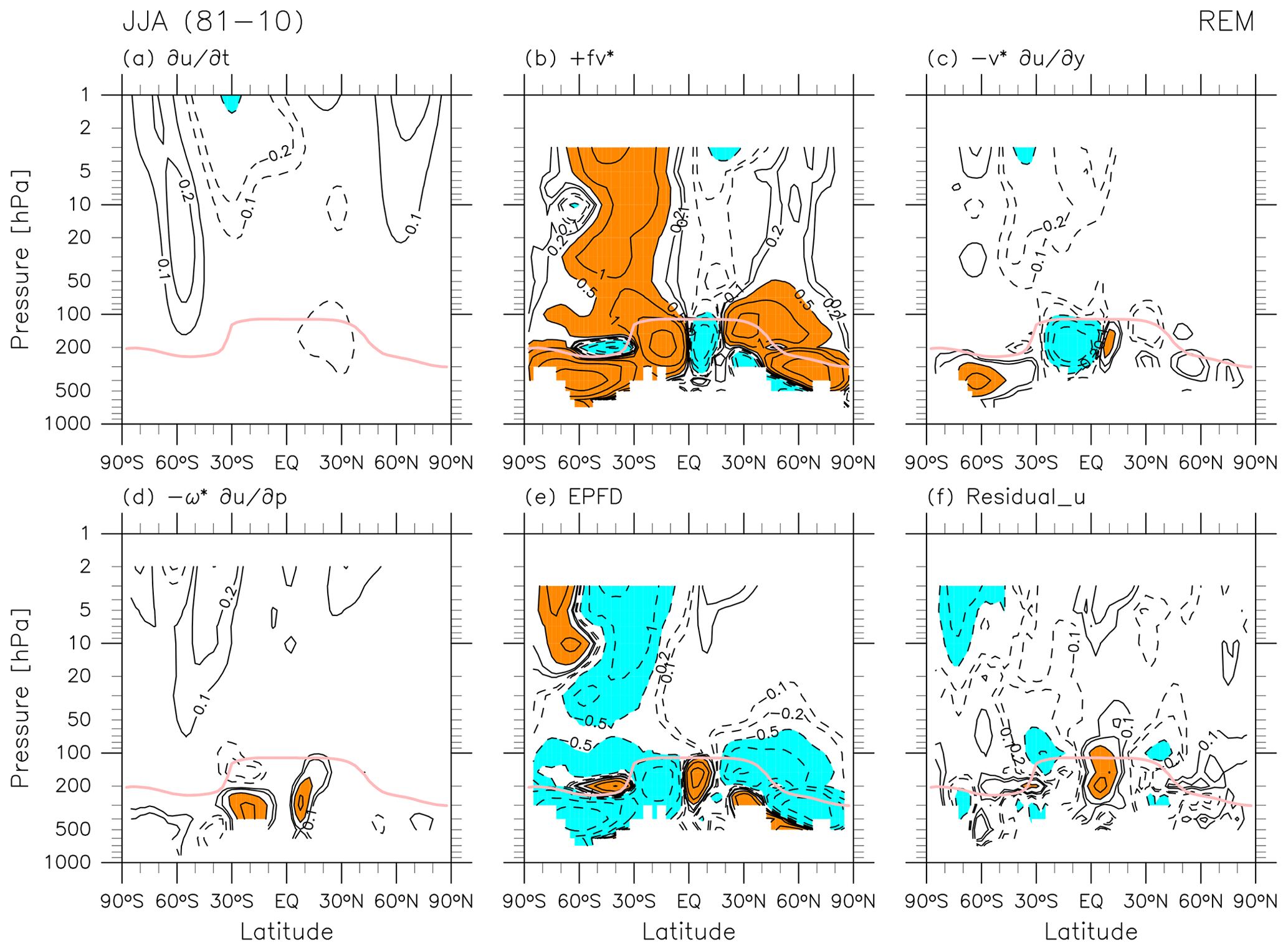
Figure 2 Latitude–pressure distributions of the REM for 30-year DJF means (December 1980–February 1981 to December 2009–February 2010) of each term in the TEM momentum equation, Eq. (4): (a) zonal wind tendency term, (b) Coriolis term, (c) meridional advection term, (d) vertical advection term, (e) EP flux divergence term, and (f) the residual term $\stackrel{\mathrm{‾}}{{\mathit{\epsilon }}_u}$. The sign of each term is defined as that shown in Eq. (4). Contours are located at ± 0.1, ± 0.2, ± 0.5, ± 1, ± 2, … m s⁻¹ d⁻¹ with dotted contours for negative values in all panels; orange shading indicates values greater than 0.5 m s⁻¹ d⁻¹, while light blue shading indicates values smaller than −0.5 m s⁻¹ d⁻¹. The pink curve in all panels shows the location of the REM DJF mean climatological tropopause.

The TEM thermodynamic equation is written as

$$\begin{array}{}\text{(5)}& \begin{array}{rl}{\displaystyle \frac{\partial \stackrel{\mathrm{‾}}{\mathit{\theta }}}{\partial t}}& =-{\stackrel{\mathrm{‾}}{v}}^{*}{\displaystyle \frac{\mathrm{1}}{a}}{\displaystyle \frac{\partial \stackrel{\mathrm{‾}}{\mathit{\theta }}}{\partial \mathit{\varphi }}}-{\stackrel{\mathrm{‾}}{\mathit{\omega }}}^{*}{\displaystyle \frac{\partial \stackrel{\mathrm{‾}}{\mathit{\theta }}}{\partial p}}-{\displaystyle \frac{\partial }{\partial p}}\left({\displaystyle \frac{\stackrel{\mathrm{‾}}{v{}^{\prime }\mathit{\theta }{}^{\prime }}\frac{\partial \stackrel{\mathrm{‾}}{\mathit{\theta }}}{\partial \mathit{\varphi }}}{a\frac{\partial \stackrel{\mathrm{‾}}{\mathit{\theta }}}{\partial p}}}+\stackrel{\mathrm{‾}}{\mathit{\omega }{}^{\prime }\mathit{\theta }{}^{\prime }}\right)\\ & +\stackrel{\mathrm{‾}}{Q_{\mathrm{total}}}+\stackrel{\mathrm{‾}}{{\mathit{\epsilon }}_{\mathit{\theta }}},\end{array}\end{array}$$

where $\stackrel{\mathrm{‾}}{Q_{\mathrm{total}}}$ is the zonal mean total diabatic heating due to either physical parameterizations (MERRA-2, ERA-Interim, and CFSR) or the sum of all diabatic heating terms provided by the reanalysis product (JRA-55) (see also Sect. 2.1) and $\stackrel{\mathrm{‾}}{{\mathit{\epsilon }}_{\mathit{\theta }}}$ is the residual term which includes the effects of analysis increments, effects associated with using pressure-level data, and errors in the numerical methods. The summation of the first three terms on the right-hand side of this equation is mathematically equivalent to the summation of the second to fourth terms on the left-hand side of Eq. (12) in Martineau et al. (2018), which is the Eulerian mean, not TEM. The M22 RID dataset includes all terms of Eq. (5) except for Q_total and $\stackrel{\mathrm{‾}}{{\mathit{\epsilon }}_{\mathit{\theta }}}$. For Q_total, we use the W17 dataset (see Martineau et al., 2018). $\stackrel{\mathrm{‾}}{{\mathit{\epsilon }}_{\mathit{\theta }}}$ is calculated in this paper as the residual from all other terms of Eq. (5) based on monthly means. The residual term $\stackrel{\mathrm{‾}}{{\mathit{\epsilon }}_{\mathit{\theta }}}$ is mathematically the same as $\stackrel{\mathrm{‾}}{\mathit{\chi }}$ in Eq. (12) of Martineau et al. (2018), although they are numerically different (see Folder 1 in the Supplement) owing to numerical differences between the summation of the first three terms on the right-hand side of Eq. (5) and the summation of the second to fourth terms on the left-hand side of Eq. (12) in Martineau et al. (2018).

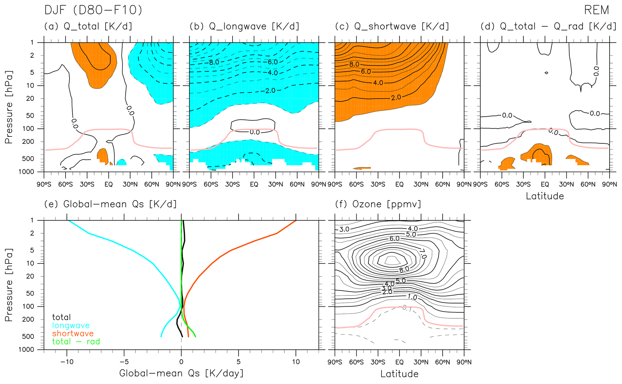
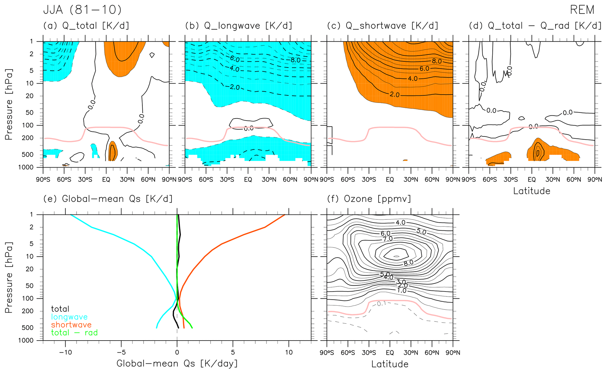
Figure 3 Latitude–pressure distributions of the REM for 30-year DJF means (December 1980–February 1981 to December 2009–February 2010) of zonal mean (a) total diabatic heating (in terms of temperature, not potential temperature; the same for b–e), (b) longwave radiative heating, (c) shortwave radiative heating, and (d) diabatic heating due to processes other than radiative transfer. The contour interval in (a–d) is 1 K d⁻¹, with dotted contours for negative values; regions with values greater than +1 K d⁻¹ are coloured in orange, while those with values smaller than −1 K d⁻¹ are coloured in light blue. The pink curve in all panels shows the location of the REM DJF mean climatological tropopause. (e) Vertical distribution of global-mean diabatic heating (black: total; light blue: longwave radiative; orange: shortwave radiative; light green: other than radiative). (f) As for (a), but for ozone mixing ratio (contour interval is 0.5 parts per million by volume (ppmv), with the 0.1 and 0.05 ppmv contours shown as dotted lines).

Considering the TEM continuity equation,

$$\begin{array}{}\text{(6)}& {\displaystyle \frac{\mathrm{1}}{a\cos \mathit{\varphi }}}{\displaystyle \frac{\partial }{\partial \mathit{\varphi }}}\left({\stackrel{\mathrm{‾}}{v}}^{*}\cos \mathit{\varphi }\right)+{\displaystyle \frac{\partial {\stackrel{\mathrm{‾}}{\mathit{\omega }}}^{*}}{\partial p}}=\mathrm{0},\end{array}$$

we can define a streamfunction ${\mathrm{\Psi }}_p^{*}$ for pressure coordinates (in units of Pa m s⁻¹) as

$$\begin{array}{}\text{(7)}& {\displaystyle }{\stackrel{\mathrm{‾}}{v}}^{*}=+{\displaystyle \frac{\mathrm{1}}{\cos \mathit{\varphi }}}{\displaystyle \frac{\partial {\mathrm{\Psi }}_p^{*}}{\partial p}},\text{(8)}& {\displaystyle }{\stackrel{\mathrm{‾}}{\mathit{\omega }}}^{*}=-{\displaystyle \frac{\mathrm{1}}{a\cos \mathit{\varphi }}}{\displaystyle \frac{\partial {\mathrm{\Psi }}_p^{*}}{\partial \mathit{\varphi }}}.\end{array}$$

Therefore, with appropriate boundary conditions, we can calculate ${\mathrm{\Psi }}_p^{*}$ from one of the following:

$$\begin{array}{}\text{(9)}& {\displaystyle }{\mathrm{\Psi }}_p^{*}=+\cos \mathit{\varphi }{\int }_{\mathrm{TOA}}^p{\stackrel{\mathrm{‾}}{v}}^{*}\mathrm{d}p{}^{\prime },\text{(10)}& {\displaystyle }{\mathrm{\Psi }}_p^{*}=-a{\int }_{\mathrm{SP}}^{\mathit{\varphi }}{\stackrel{\mathrm{‾}}{\mathit{\omega }}}^{*}\mathrm{d}\mathit{\varphi }{}^{\prime },\text{(11)}& {\displaystyle }{\mathrm{\Psi }}_p^{*}=-a{\int }_{\mathrm{NP}}^{\mathit{\varphi }}{\stackrel{\mathrm{‾}}{\mathit{\omega }}}^{*}\mathrm{d}\mathit{\varphi }{}^{\prime },\end{array}$$

where TOA stands for the nominal top of atmosphere, SP for the South Pole, and NP for the North Pole (note that dϕ^′ is negative in Eq. 11). ${\mathrm{\Psi }}_p^{*}$ calculated from ${\stackrel{\mathrm{‾}}{v}}^{*}$ is often used in middle-atmosphere studies (e.g. Abalos et al., 2015) because ${\stackrel{\mathrm{‾}}{v}}^{*}$ data may be more reliable than ${\stackrel{\mathrm{‾}}{\mathit{\omega }}}^{*}$ in reanalysis data (as meridional wind observations are assimilated, while vertical winds are not). On the other hand, values of ${\mathrm{\Psi }}_p^{*}$ calculated from ${\stackrel{\mathrm{‾}}{v}}^{*}$ are rather sensitive to the treatment of upper-boundary conditions (i.e. TOA in the integral); in some cases they are sensitive even down to the lower stratosphere depending on the height of the top data level. Thus, some works (e.g. Sato and Hirano, 2019) use ${\mathrm{\Psi }}_p^{*}$ calculated from ${\stackrel{\mathrm{‾}}{\mathit{\omega }}}^{*}$. In this paper, we calculate both streamfunctions and compare the two. When calculating ${\mathrm{\Psi }}_p^{*}$ calculated from ${\stackrel{\mathrm{‾}}{v}}^{*}$, we follow Chapter 5 of SPARC (2022, Sect. 5.2.1) for the treatment of the upper boundary (i.e. TOA in the integral). In short, we create monthly ${\stackrel{\mathrm{‾}}{v}}^{*}$ data at the top two levels (1 and 2 hPa for the common grid dataset), where they are missing in M17, by extrapolation and with some assumptions. We then set the top boundary conditions to 0 hPa and the 0–1 hPa layer so that the average ${\stackrel{\mathrm{‾}}{v}}^{*}$ for the 0–1 hPa layer is half the ${\stackrel{\mathrm{‾}}{v}}^{*}$ at 1 hPa, which corresponds to setting ${\stackrel{\mathrm{‾}}{v}}^{*}=\mathrm{0}$ at 0 hPa. For ${\mathrm{\Psi }}_p^{*}$ calculated from ${\stackrel{\mathrm{‾}}{\mathit{\omega }}}^{*}$, we use Eq. (10) for the Southern Hemisphere (SH) and Eq. (11) for the Northern Hemisphere (NH) and set values at the Equator to the average of the values calculated using Eqs. (10) and (11).

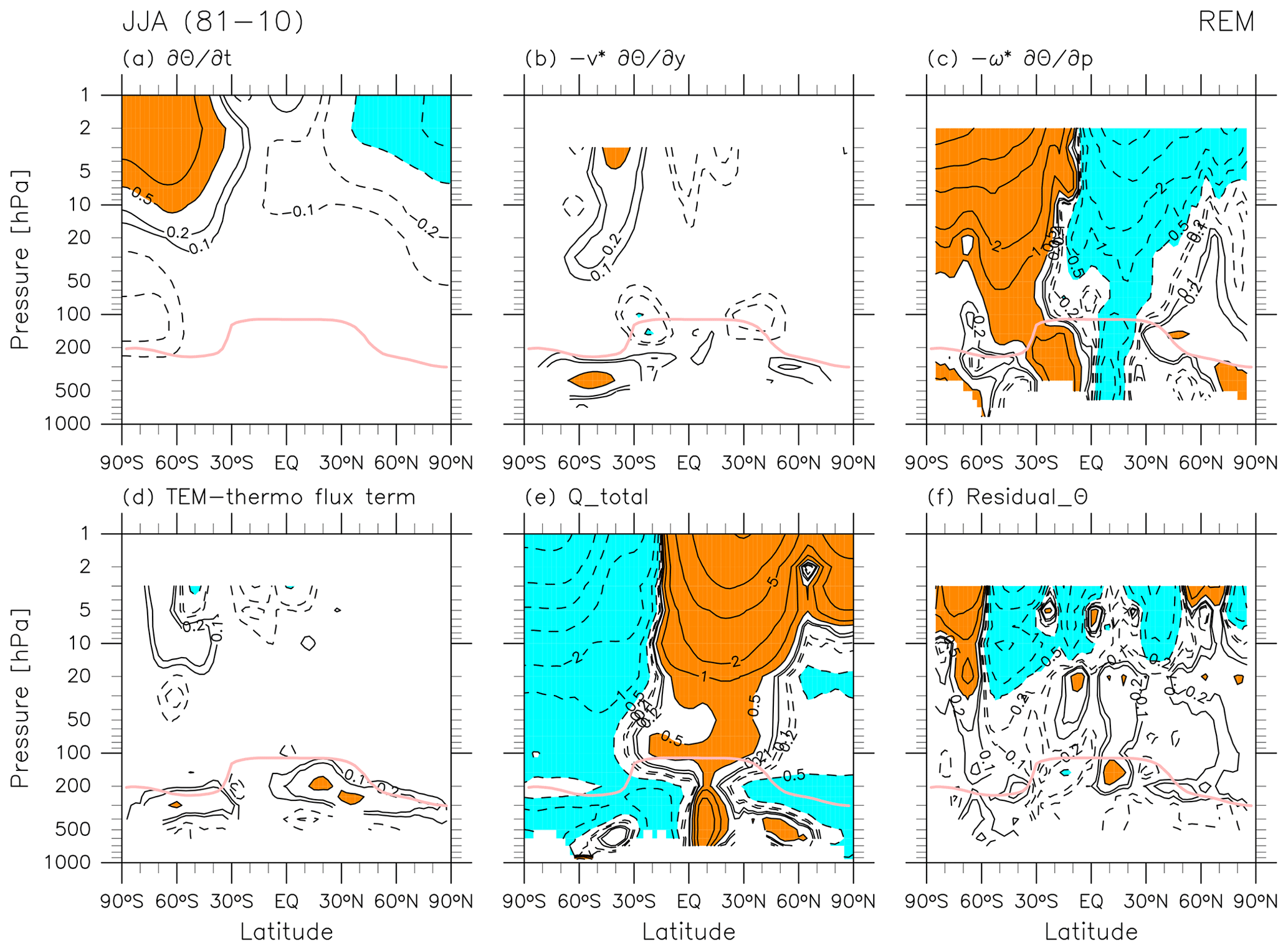
Figure 4 Latitude–pressure distributions of the REM for 30-year DJF means (December 1980–February 1981 to December 2009–February 2010) of each term in the TEM thermodynamic equation, Eq. (5): (a) potential temperature tendency term, (b) meridional advection term, (c) vertical advection term, (d) wave flux term (the third term of right-hand side of Eq. 5), (e) total diabatic heating term, and (f) the residual term $\stackrel{\mathrm{‾}}{{\mathit{\epsilon }}_{\mathit{\theta }}}$. The sign of each term is defined as in Eq. (5). Contours are located at ± 0.1, ± 0.2, ± 0.5, ± 1, ± 2, … K d⁻¹ with dotted contours for negative values in all panels; orange shading indicates values greater than 0.5 K d⁻¹, while light blue shading indicates values smaller than −0.5 K d⁻¹. The pink curve in all panels shows the location of the REM DJF mean climatological tropopause.

In Sect. 3, as for many previous studies (e.g. Abalos et al., 2015; Sato and Hirano, 2019; Chapter 5 of SPARC, 2022), the streamfunction in log-pressure coordinates (i.e. the mass streamfunction Ψ^*) is shown in units of kilograms per metre per second (kg m⁻¹ s⁻¹). Conversion to the mass streamfunction is accomplished by

$$\begin{array}{}\text{(12)}& {\mathrm{\Psi }}^{*}={\displaystyle \frac{H}{R{T}_s}}{\mathrm{\Psi }}_p^{*}={\displaystyle \frac{\mathrm{1}}{g_{\mathrm{0}}}}{\mathrm{\Psi }}_p^{*},\end{array}$$

where R is the gas constant for dry air, T_s is a constant reference temperature set as 240 K, and g₀ is the global average gravitational constant at mean sea level (Andrews et al., 1987, their Sects. 1.1.1 and 3.1.1). Hereafter, the mass streamfunction calculated from ${\stackrel{\mathrm{‾}}{v}}^{*}$ is referred to as ${\mathrm{\Psi }}_{{\stackrel{\mathrm{‾}}{v}}^{*}}^{*}$ and that calculated from ${\stackrel{\mathrm{‾}}{\mathit{\omega }}}^{*}$ as ${\mathrm{\Psi }}_{{\stackrel{\mathrm{‾}}{\mathit{\omega }}}^{*}}^{*}$.

Finally, we also calculate ${\stackrel{\mathrm{‾}}{\mathit{\omega }}}^{*}$ and ${\stackrel{\mathrm{‾}}{w}}^{*}$ from ${\mathrm{\Psi }}_{{\stackrel{\mathrm{‾}}{v}}^{*}}^{*}$ through Eqs. (8) and (3) (${\stackrel{\mathrm{‾}}{\mathit{\omega }}}_{{\stackrel{\mathrm{‾}}{v}}^{*}}^{*}$ and ${\stackrel{\mathrm{‾}}{w}}_{{\stackrel{\mathrm{‾}}{v}}^{*}}^{*}$, respectively) and compare them with the original ${\stackrel{\mathrm{‾}}{\mathit{\omega }}}^{*}$ and ${\stackrel{\mathrm{‾}}{w}}^{*}$ in Sect. 3.

2.3 Climatological tropopause location

The climatological latitudinal distribution of tropopause pressure is shown in the figures in Sect. 3. The tropopause is defined here as the lowermost location above 5 km altitude where the magnitude of the temperature decrease with respect to log-pressure height ($z=-H\ln (p/p_s$), with p_s=10⁵ Pa) becomes less than 2 K km⁻¹, using linear interpolation to estimate the exact point. The same definition is used for all latitudes. We use 30-year (1981–2010) climatological mean temperature distributions from monthly averaged common grid reanalysis data to determine climatological tropopause locations. Therefore, the tropopause as shown in the following figures is for illustrative purposes only.

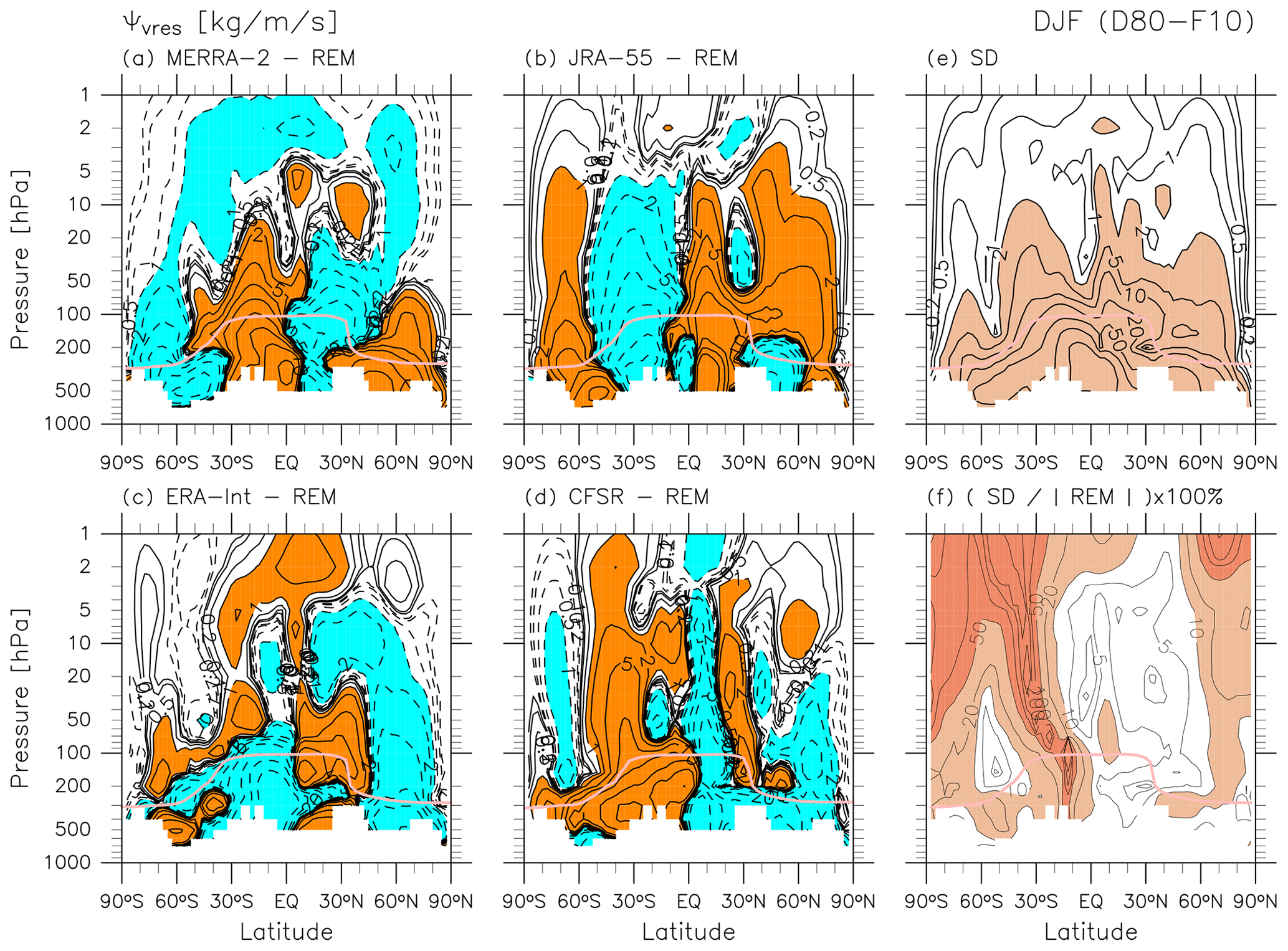
Figure 5 Latitude–pressure distributions of 30-year DJF means (December 1980–February 1981 to December 2009–February 2010) of the ${\mathrm{\Psi }}_{{\stackrel{\mathrm{‾}}{v}}^{*}}^{*}$ anomaly with respect to the REM for (a) MERRA-2, (b) JRA-55, (c) ERA-Interim, and (d) CFSR. Contours are located at ± 0.1, ± 0.2, ± 0.5, ± 1, ± 2, … kg m⁻¹ s⁻¹ with dotted contours for negative values in all panels; orange shading indicates values greater than 1 kg m⁻¹ s⁻¹, while light blue shading indicates values smaller than −1 kg m⁻¹ s⁻¹. (e) Inter-reanalysis differences for ${\mathrm{\Psi }}_{{\stackrel{\mathrm{‾}}{v}}^{*}}^{*}$ presented as standard deviation (SD; contours at 0.1, 0.2, 0.5, 1, 2, … kg m⁻¹ s⁻¹; light red shading for values greater than 2 kg m⁻¹ s⁻¹). (f) Inter-reanalysis differences for ${\mathrm{\Psi }}_{{\stackrel{\mathrm{‾}}{v}}^{*}}^{*}$ presented as SD divided by the absolute value of the REM in percent (contours are at 1, 2, 5, 10, 20, …%, light red shading marks values greater than 10 %, and dark red shading marks values greater than 50 %). The pink curve in all panels shows the location of the DJF mean climatological tropopause for each reanalysis in panels (a)–(d) and for the REM in panels (e) and (f).

3 Results and discussion

3.1 DJF

3.1.1 REM for DJF

Figure 1 shows the REM climatological latitude–pressure distributions of the TEM variables for DJF. Values in the lower troposphere are often missing because MERRA-2 does not provide pressure-level data below the Earth surface and because zonal means were not calculated in M22 for latitude bands with one or more missing data points in longitude. During DJF, the tropical tropopause is colder than all other seasons, and the NH polar stratosphere is colder than the SH polar stratosphere. The distributions of temperature and zonal wind agree quite well with the thermal wind balance in the zonal mean (not shown directly). The residual mean meridional circulation (i.e. the advective part of the stratospheric BD circulation) shows the following characteristics: (1) upwelling in the tropics (with two local maxima around 70–50 hPa – one around 12.5° N and the other around 15° S – and a minimum in the equatorial lower stratosphere; note that the closed contours around 70–30 hPa at the Equator in ${\stackrel{\mathrm{‾}}{w}}^{*}$ show a minimum; see also Chapter 5 of SPARC, 2022, their Figs. 5.2 and 5.5); (2) poleward flow in the stratosphere, i.e. northward flow in the NH and southward flow in the SH; and (3) downwelling in the extratropics. The NH northward flow is much stronger than the SH southward flow during DJF. The ${\stackrel{\mathrm{‾}}{v}}^{*}$ distribution also clearly shows the shallow branches of the BD circulation in the mid-latitude lower stratosphere (200–100 hPa in NH and 200–50 hPa in SH). Within these distributions, we also see the upper-tropospheric branch of the Hadley cells in the tropics, with the tropical-to-NH (clockwise) cell being stronger during DJF (see e.g. Schneider and Bordoni, 2008). Equatorward flow along the mid-latitude tropopause in both hemispheres is evident in all four reanalyses (see Folder 2 in the Supplement) and is associated with EP flux divergence due to resolved waves there (see Fig. 2) as discussed by Birner et al. (2013).

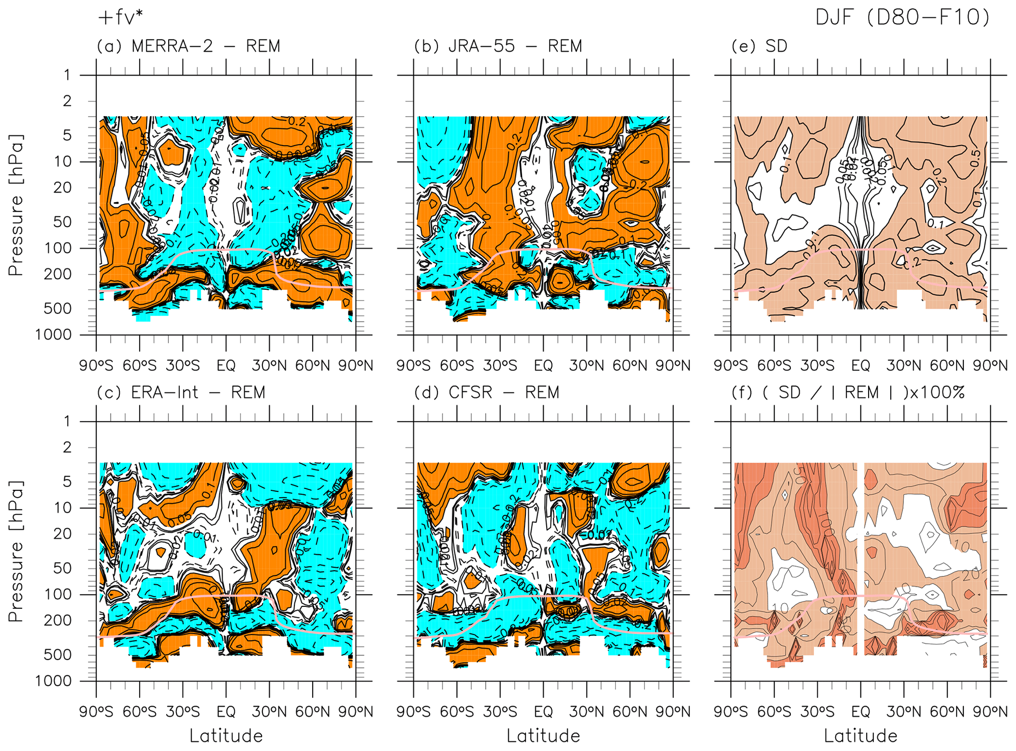
Figure 6 As for Fig. 5, but for the Coriolis term. For (a–e), contours are located at ± 0.01, ± 0.02, ± 0.05, ± 0.1, ± 0.2, … m s⁻¹ d⁻¹ with dotted contours for negative values in all panels. For (a–d), orange shading indicates values greater than 0.05 m s⁻¹ d⁻¹, while light blue shading indicates values smaller than −0.05 m s⁻¹ d⁻¹. For (e), light red shading marks values greater than 0.1 m s⁻¹ d⁻¹. For (f), contours are located at 1, 2, 5, 10, 20, …%, light red shading marks values greater than 10 %, and dark red shading marks values greater than 50 %.

Figure 1 also compares ${\stackrel{\mathrm{‾}}{w}}^{*}$ and ${\stackrel{\mathrm{‾}}{w}}_{{\stackrel{\mathrm{‾}}{v}}^{*}}^{*}$, the latter of which is estimated from ${\stackrel{\mathrm{‾}}{v}}^{*}$ through the streamfunction calculation (i.e. through the continuity equation). The two vertical velocity fields show reasonable agreement in the troposphere and in the lower stratosphere up to 10 hPa, but differences even with this roughly logarithmic contouring are evident in the upper stratosphere. In general, reanalysis meridional wind products are strongly constrained by observations through data assimilation. By contrast, vertical velocities in reanalysis products are highly dependent on the specific implementation of data assimilation. For example, in early reanalyses using 3-dimensional variational (3D-Var) assimilation, vertical winds are primarily determined by the underlying forecast model (e.g. Sect. 6 of Kalnay et al., 1996). In more recent reanalysis systems using 4D-Var assimilation techniques, vertical velocities are influenced by observational data indirectly through data assimilation constraints on horizontal winds. Because vertical velocities are small and computed indirectly from horizontal divergence, even small assimilation increments in horizontal winds can have large influences on vertical velocities (Uma et al., 2021). These effects can produce substantial noise in reanalysis estimates of vertical velocity (Wohltmann and Rex, 2008; Hoffmann et al., 2019). Monge-Sanz et al. (2007, 2012) showed how advances in the assimilation schemes resulted in more realistic vertical wind fields and also that improvements were still needed. Therefore, estimates of ${\stackrel{\mathrm{‾}}{\mathit{\omega }}}^{*}$ and ${\stackrel{\mathrm{‾}}{w}}^{*}$ from ${\stackrel{\mathrm{‾}}{v}}^{*}$ may still be more reliable for studies of particular atmospheric processes in particular regions. It should be noted that estimation through the streamfunction has its own issues, as the streamfunction from Eq. (9) is sensitive to conditions applied for the “TOA” (including the choice of the data top, e.g. 1 hPa versus 0.1 hPa) even down to the lower stratosphere. Therefore, looking at both estimates of residual vertical velocity and trusting only the common features may be a good approach. Note also that in this paper we use the common grid dataset for which the top is located at 1 hPa for the purpose of comparisons of different reanalyses. The use of original grid data (or model-level data) with higher tops would improve estimates of ${\stackrel{\mathrm{‾}}{\mathit{\omega }}}^{*}$ and ${\stackrel{\mathrm{‾}}{w}}^{*}$ from ${\stackrel{\mathrm{‾}}{v}}^{*}$.

Figure 1 also shows and compares the two streamfunctions ${\mathrm{\Psi }}_{{\stackrel{\mathrm{‾}}{v}}^{*}}^{*}$ and ${\mathrm{\Psi }}_{{\stackrel{\mathrm{‾}}{\mathit{\omega }}}^{*}}^{*}$ (see Sect. 2.2 for the details). During DJF, the NH cells for both the BD circulation and the Hadley circulation are more pronounced than their SH counterparts. This is in overall agreement with the results from Michelson Interferometer for Passive Atmospheric Sounding (MIPAS) satellite observations (von Clarmann et al., 2021), with a cautionary note that their climatology was computed for the shorter period 2002–2012. We also note quantitative differences between the two streamfunctions with a roughly logarithmic contouring in Fig. 1 not only in the upper stratosphere (above the 10 hPa level) but also in the lower stratosphere. These differences arise due to the reasons discussed in the previous paragraph.

Figure 7 As for Fig. 6, but for the EP flux divergence term.

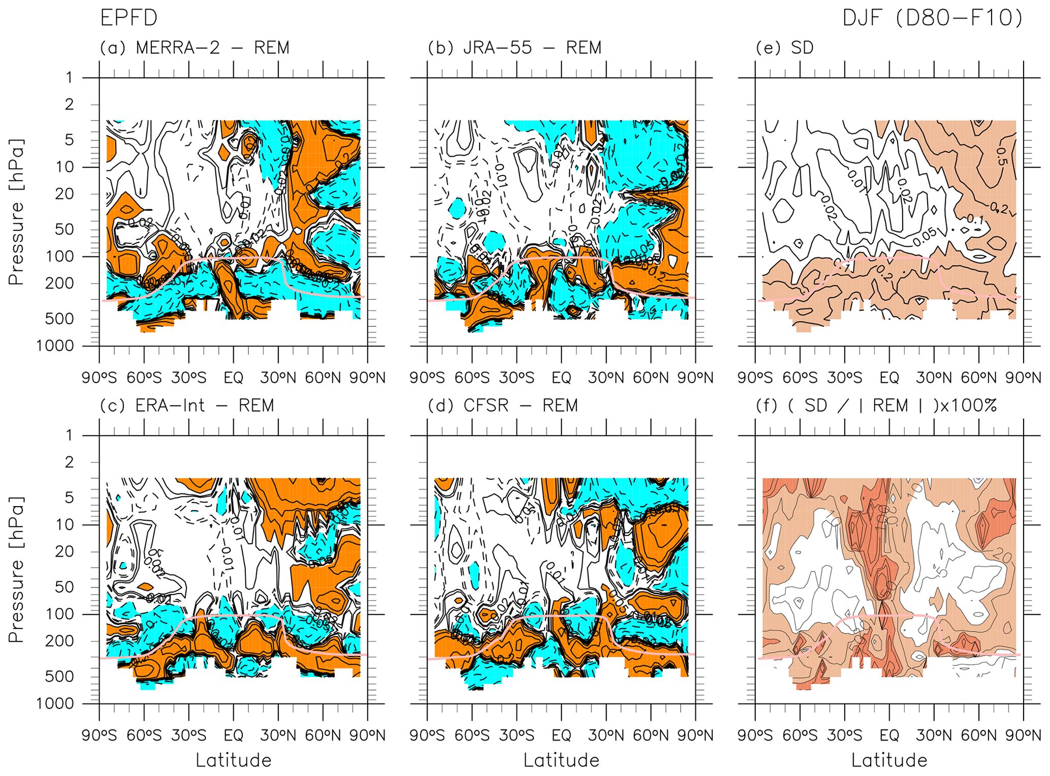
Figure 2 shows the REM climatological distributions of all terms in the TEM momentum equation, Eq. (4) (in units of m s⁻¹ d⁻¹), for DJF. The sign of each term is defined as in Eq. (4). The major terms in the stratosphere at monthly timescales are the Coriolis term and the EP flux divergence term (the latter due to resolved waves), with strong signals extending much higher in the NH than in the SH during this season. These results illustrate the main mechanisms driving the BD circulation, namely that EP flux convergence arising mainly from the dissipation of upward-propagating Rossby waves in the extratropical stratosphere and synoptic-scale waves in the subtropical lower stratosphere results in poleward flow (Sect. 4 of Butchart, 2014). During DJF, the existence of a polar night jet in the NH (Fig. 1c) enables Rossby waves to propagate higher in the NH stratosphere, producing greater EP flux convergence and driving stronger poleward flow in the NH. Along the mid-latitude tropopause in both hemispheres (around 40° N and 200 hPa and around 50–60° S and 200–300 hPa), signals in the EP flux divergence due to resolved waves correspond to equatorward flow (see Figs. 1d, 2b, and 2e; Birner et al., 2013). The momentum balance in the troposphere is more complicated in this TEM framework, with additional contributions from the meridional and vertical advection terms. As noted in Sect. 2.2, the residual term $\stackrel{\mathrm{‾}}{{\mathit{\epsilon }}_u}$ includes the effects of parameterized processes such as gravity waves, convective processes, turbulent and numerical diffusion, errors in the numerical methods, and adjustments arising from analysis increments. The main contribution to $\stackrel{\mathrm{‾}}{{\mathit{\epsilon }}_u}$ in the stratosphere comes from the forcing due to dissipating gravity waves (Sato and Hirano, 2019), while contributions from diffusion and cloud processes may also be important in the troposphere (see Folder 4 in the Supplement for investigation of zonal accelerations due to the parameterizations provided for the four reanalysis datasets). Negative signals in $\stackrel{\mathrm{‾}}{{\mathit{\epsilon }}_u}$ in the mid-latitude lower stratosphere may result in part from unresolved forcing due to gravity waves generated by the subtropical jets (e.g. Kawatani et al., 2004; Plougonven and Snyder, 2007) and the orography (e.g. Kuchar et al., 2020). See also Podglajen et al. (2020) for a comparison of reanalyses with long-duration, quasi-Lagrangian balloon observations in the equatorial and Antarctic lower stratosphere with respect to gravity wave spectra. We also find negative signals in $\stackrel{\mathrm{‾}}{{\mathit{\epsilon }}_u}$ in the NH high-latitude upper stratosphere, which may result in part from gravity waves generated by the winter polar night jet and the orography.

Figure 3 shows REM climatological distributions of diabatic heating for DJF, with particular attention to the radiative heating. Note that all heating terms shown in Fig. 3 are with respect to temperature tendency, not potential temperature tendency, to facilitate comparison with the previous literature. Andrews et al. (1987, Chapter 2) discuss radiative heating in the stratosphere and lower mesosphere based on results from e.g. Kiehl and Solomon (1986), who used radiative transfer models and satellite observations of temperature and ozone. More recent assessments of middle-atmosphere radiative heating include those by Gettelman et al. (2004), Fueglistaler et al. (2009), SPARC (2010, Chapter 3), Ming et al. (2016), and Tao et al. (2019; their Fig. 3). For LW heating, major contributions in the stratosphere include cooling to space by CO₂ (roughly three-fourths) and O₃ (roughly a fourth), with that by H₂O having a non-negligible contribution (Andrews et al., 1987, their Fig. 2.1). Weak positive LW heating around the tropical tropopause region is due to absorption of fluxes from below by O₃. Negative LW heating in the troposphere is mainly attributable to H₂O. For SW heating, absorption by O₃ is the major component in the stratosphere, together with the latitudinal and seasonal distribution of solar insolation at the TOA, which is much greater in the SH than in the NH during DJF (see e.g. Liou, 2002). The REM ozone distribution for DJF is also shown in Fig. 3 for reference (see the caveat for ERA-Interim in the last paragraph of Sect. 2.1). Other components of diabatic heating include convective heating and large-scale condensation heating, primarily in the troposphere; heating by turbulent mixing in regions of shear-flow instability; and heating due to parameterized gravity waves (depending on the parameterized scheme). In the stratosphere, the distribution of the total diabatic heating is almost entirely determined by the balance between LW cooling and SW heating (Fig. 3d–e). Although the total diabatic heating is nearly zero in the global mean (Fig. 3e), during DJF it comprises heating in the SH stratosphere and cooling in the NH stratosphere.

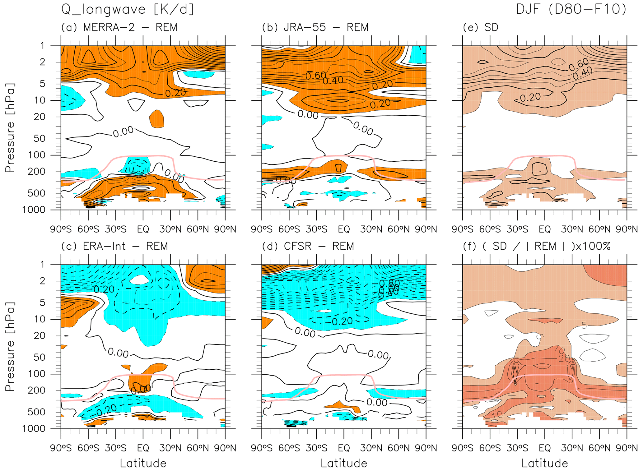
Figure 8 As for Fig. 5, but for longwave radiative heating. For (a–e), the contour interval is 0.1 K d⁻¹ with dotted contours for negative values in all panels. For (a–d), orange shading indicates values greater than 0.1 K d⁻¹, while light blue shading indicates values smaller than −0.1 K d⁻¹. For (e), light red shading marks values greater than 0.1 K d⁻¹. For (f), contours are located at 1, 2, 5, 10, 20, …%, light red shading marks values greater than 5 %, and dark red shading marks values greater than 10 %.

Figure 4 shows REM climatological distributions of all terms in the TEM thermodynamic equation, Eq. (5) (in units of K d⁻¹), during DJF. The sign of each term is defined as in Eq. (5). The major terms in the stratosphere at monthly timescales are the vertical advection term and the total diabatic heating term (essentially radiative heating, as shown in Fig. 3), but other terms show noticeable contributions at higher latitudes in the middle-to-upper stratosphere. Most notably, values of the residual term $\stackrel{\mathrm{‾}}{{\mathit{\epsilon }}_{\mathit{\theta }}}$ are on the same order of magnitude as those for the two major terms in the NH stratosphere during DJF. As noted in Sects. 1 and 2.2, the main component of $\stackrel{\mathrm{‾}}{{\mathit{\epsilon }}_{\mathit{\theta }}}$ is the analysis increment, defined as the difference between the analysis state and the first-guess (forecast) background state. Figure 4f indicates that there are large differences between the observationally constrained analysis and the forecast model in the NH mid-to-upper stratosphere during DJF.

Figure 9 As for Fig. 8, but for shortwave radiative heating.

3.1.2 Differences in each reanalysis from the REM for DJF

The variables and terms discussed in this section include the mass streamfunction of the residual mean meridional circulation calculated from ${\stackrel{\mathrm{‾}}{v}}^{*}$ (${\mathrm{\Psi }}_{{\stackrel{\mathrm{‾}}{v}}^{*}}^{*}$), the two major terms of the TEM momentum equation, LW and SW radiative heating, and the two major terms of the TEM thermodynamic equation. Differences with respect to the REM for each reanalysis are shown in the following figures, along with inter-reanalysis spreads presented as standard deviation (SD) and relative SD (i.e. SD divided by the absolute value of REM). See Folder 3 in the Supplement for other major TEM variables and terms including temperature and zonal wind. For temperature, differences among different reanalyses become greater at higher altitudes because of weaker observational constraints. In the upper stratosphere, JRA-55 is colder than the REM, and CFSR is warmer, with MERRA-2 and ERA-Interim in the middle. For zonal wind, the differences are largest in the tropics (because of a weaker thermal wind constraint) and in the low-to-mid-latitude upper stratosphere, as also shown in Chapters 3 and 11 of SPARC (2022).

Figure 5 shows differences for the mass streamfunction ${\mathrm{\Psi }}_{{\stackrel{\mathrm{‾}}{v}}^{*}}^{*}$ during DJF. The differences change sign across latitudes, suggesting differences in the structure of the residual mean meridional circulation among different reanalyses (e.g. the separation location between the shallow and deep branches). In the lower stratosphere below the 10 hPa level, the main (NH) cell of the BD circulation (Fig. 1g) is generally stronger for JRA-55 and weaker for MERRA-2. This discrepancy can also be seen in the distributions of ${\stackrel{\mathrm{‾}}{v}}^{*}$ based on these two reanalyses (Folder 3 in the Supplement). Inter-reanalysis standard deviations relative to the REM (Fig. 5f) indicate differences of 2 %–10 % among these reanalyses in the main (NH) cell of the BD circulation. Note that these fractional differences can be quite large in regions where the REM is close to zero; thus we must always refer back to the REM distribution to identify the important regions. The features for ${\mathrm{\Psi }}_{{\stackrel{\mathrm{‾}}{v}}^{*}}^{*}$ described above are generally in good agreement with those for ${\mathrm{\Psi }}_{{\stackrel{\mathrm{‾}}{\mathit{\omega }}}^{*}}^{*}$ (Folder 3 in the Supplement). Differences in the individual components of the residual circulation (${\stackrel{\mathrm{‾}}{v}}^{*}{\stackrel{\mathrm{‾}}{w}}^{*}$) can also be found in Folder 3 in the Supplement. For example, differences in ${\stackrel{\mathrm{‾}}{w}}^{*}$ during DJF (Folder 3 in the Supplement) show vertical bands with widths of roughly 20–30° in latitude and are therefore difficult to describe concisely.

Figures 6 and 7 show differences in each reanalysis relative to the REM during DJF for the two major terms of the TEM momentum equation, i.e. the Coriolis term and the EP flux divergence term. The distribution of differences in the Coriolis term matches that of differences in ${\stackrel{\mathrm{‾}}{v}}^{*}$ (Folder 3 in the Supplement). In the mid-latitude lower stratosphere below the 10 hPa level, generally positive differences (stronger poleward flows) are found in JRA-55 and negative differences (weaker poleward flow) in MERRA-2. Figure 6f shows that inter-reanalysis fractional differences for $f{\stackrel{\mathrm{‾}}{v}}^{*}$ are generally less than 10 % in the NH extratropical stratosphere and SH lower stratosphere, where strong poleward flows are found in the REM (Fig. 1d). In the winter hemisphere where we expect wave-driven ${\stackrel{\mathrm{‾}}{v}}^{*}$, Fig. 7 shows that differences in the EP flux divergence term exhibit generally negative differences (more convergence) in JRA-55 and positive differences (less convergence) in MERRA-2. Large differences (both positive and negative) are found in the NH middle-to-upper stratosphere and in the extratropical lower stratosphere in both hemispheres, both regions where the EP flux divergence has significant values in the REM, indicating differences in Rossby and synoptic-scale wave activity across the four reanalyses. Differences in resolved wave activity in the stratosphere can be caused in part by different treatments of unresolved gravity waves in the reanalyses (see differences in the residual term in Folder 3 in the Supplement), which can affect the resolved wave field through a set of dynamical interactions termed the compensation mechanism by Cohen et al. (2013, 2014) (see also Hájková and Šácha, 2024). Moreover, Eichinger et al. (2020) have shown that the choice of gravity wave parameterization scheme in a climate model influences the resolved wave field throughout the model domain, often in the opposite sense to compensation. Inter-reanalysis fractional standard deviations are generally less than 10 % in the extratropical stratosphere (Fig. 7f). Figures 2e and 7 are complementary to Fig. 5.4 in Chapter 5 of SPARC (2022), which shows the seasonal cycles of EP flux divergence averaged for the shallow (100–70 hPa) and deep (50–3 hPa) branches of the BD circulation in the NH and SH separately. Figure 7 indicates that averaging over the whole hemisphere obscures large local inter-reanalysis differences.

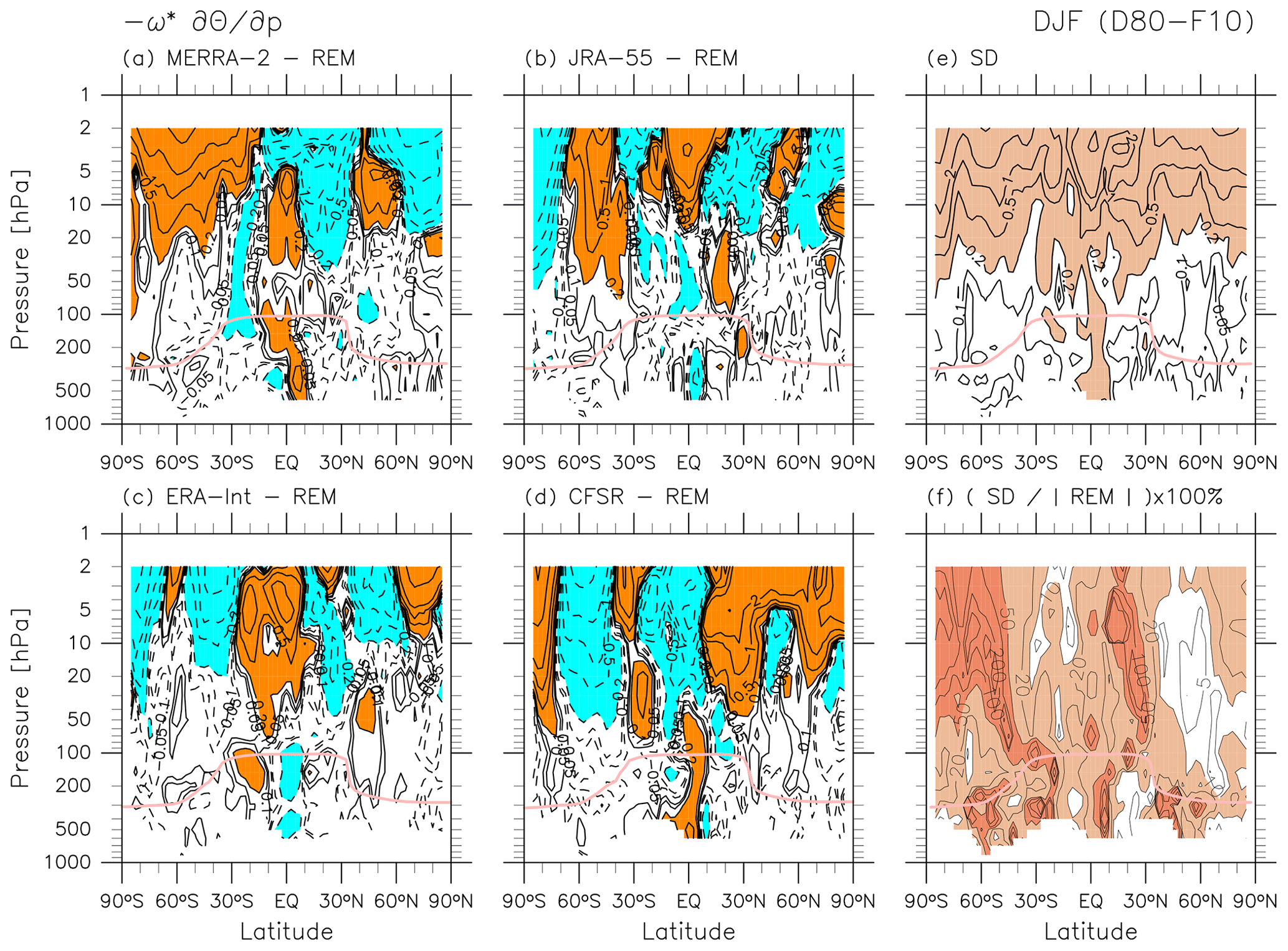
Figure 10 As for Fig. 5, but for the vertical potential temperature advection term of the TEM thermodynamic equation. For (a–e), contours are located at ± 0.05, ± 0.1, ± 0.2, ± 0.5, ± 1, … K d⁻¹ with dotted contours for negative values for all the panels. For (a–d), orange shading indicates values greater than 0.2 K d⁻¹, while light blue shading indicates values smaller than −0.2 K d⁻¹. For (e), light red shading indicates values greater than 0.2 K d⁻¹. For (f), contours are located at 1, 2, 5, 10, 20, … %, light red shading marks values greater than 10 %, and dark red shading marks values greater than 50 %.

Figure 8 shows differences in LW radiative heating during DJF. The greatest absolute differences are found in the upper stratosphere (fractional differences of 5 %–10 % generally and >10 % in the winter polar upper stratosphere), with MERRA-2 and JRA-55 being more positive than the REM and ERA-Interim and CFSR being more negative. Strong negative differences in CFSR and strong positive differences in JRA-55 are consistent with temperature differences between these two reanalyses, i.e. warmer in CFSR and colder in JRA-55 (Folder 3 in the Supplement; Chapter 3 of SPARC, 2022). In the middle atmosphere, the cooling-to-space (or Newtonian cooling) approximation works well to explain the dependence of LW radiative cooling on local temperature (e.g. Liou, 2002, their Sect. 4.5.2). Thus, the differences in LW heating in the upper stratosphere shown in Fig. 8 may be largely determined by differences in temperature. By contrast, LW heating differences in the troposphere and around the tropopause are probably related mainly to differences in the distribution of clouds (Fueglistaler and Fu, 2006; Wright et al., 2020; Chapter 8 of SPARC, 2022). Large fractional differences (10 %–50 % and even larger in some regions) are found around the tropopause globally and in the tropical-to-subtropical lower stratosphere where heating due to O₃ absorption of upwelling LW radiation fluxes from the troposphere is also important (Fig. 8f).

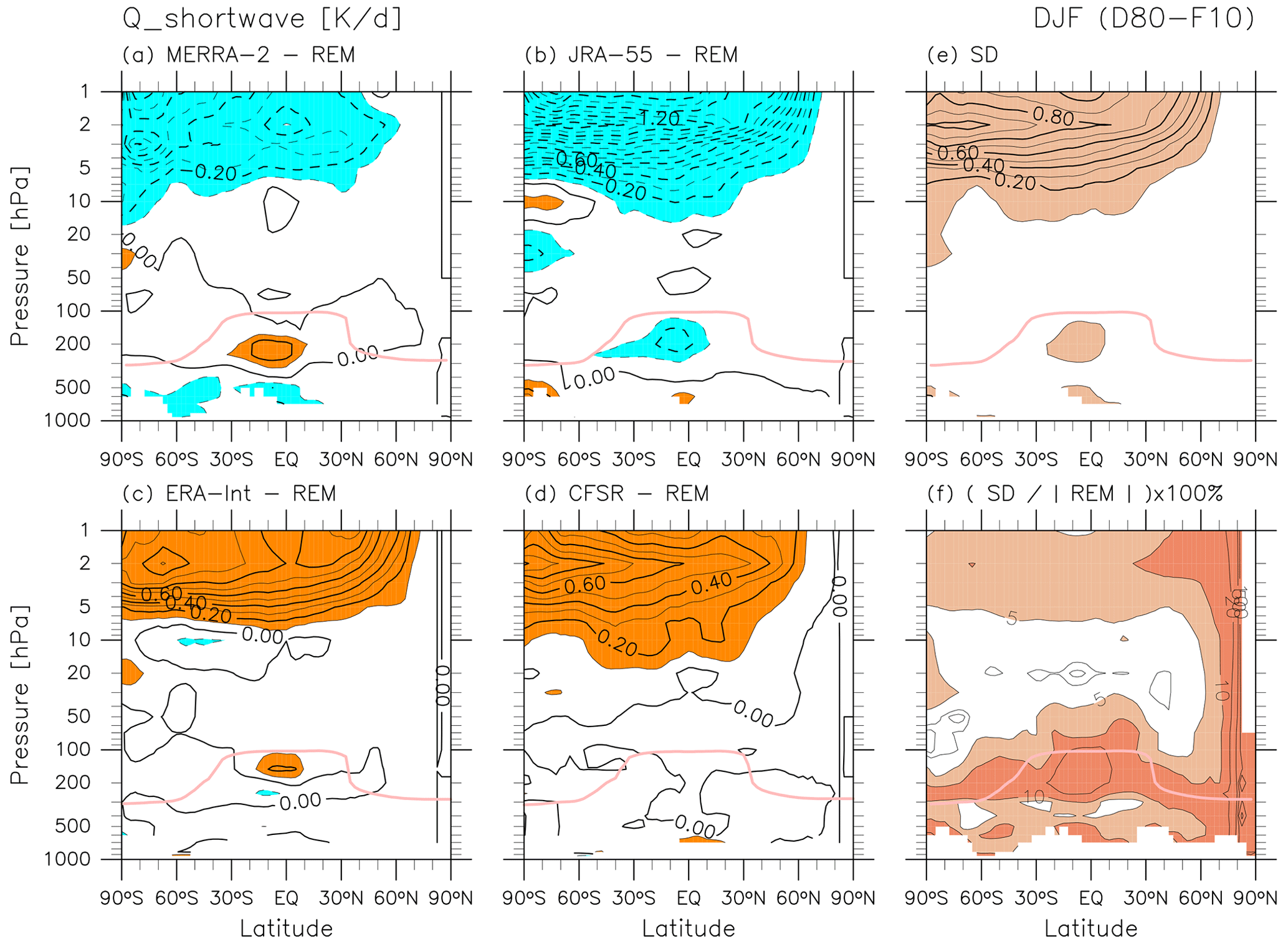
Figure 9 shows differences in SW radiative heating during DJF. The greatest absolute differences are found in the sunlit region of the upper stratosphere (fractional differences of 5 %–10 %). The strong negative differences in JRA-55 are consistent with negative differences in ozone concentration in this reanalysis relative to others (Folder 3 in the Supplement; Chapter 4 of SPARC, 2022). By contrast, strong positive differences in CFSR and negative differences in MERRA-2 cannot be fully understood from differences in ozone concentrations between these two reanalyses, implying the existence of other factors. Such factors may include details of the radiative transfer schemes, as these two forecast models use different broadband models for both SW and LW and make different assumptions for the prescribed distributions of radiatively active gases (see Chapter 2 of SPARC, 2022), both of which will impact the stratospheric radiative equilibrium in ways that are difficult to untangle. Note that ERA-Interim uses climatological ozone distributions for radiative transfer calculations. Differences in SW radiative heating in the tropical upper troposphere, where fractional differences exceed 50 %, may be related to differences in the cloud distribution (Wright et al., 2020; Chapter 8 of SPARC, 2022). Large fractional differences (10 %–50 %) are also evident around the extratropical tropopause.

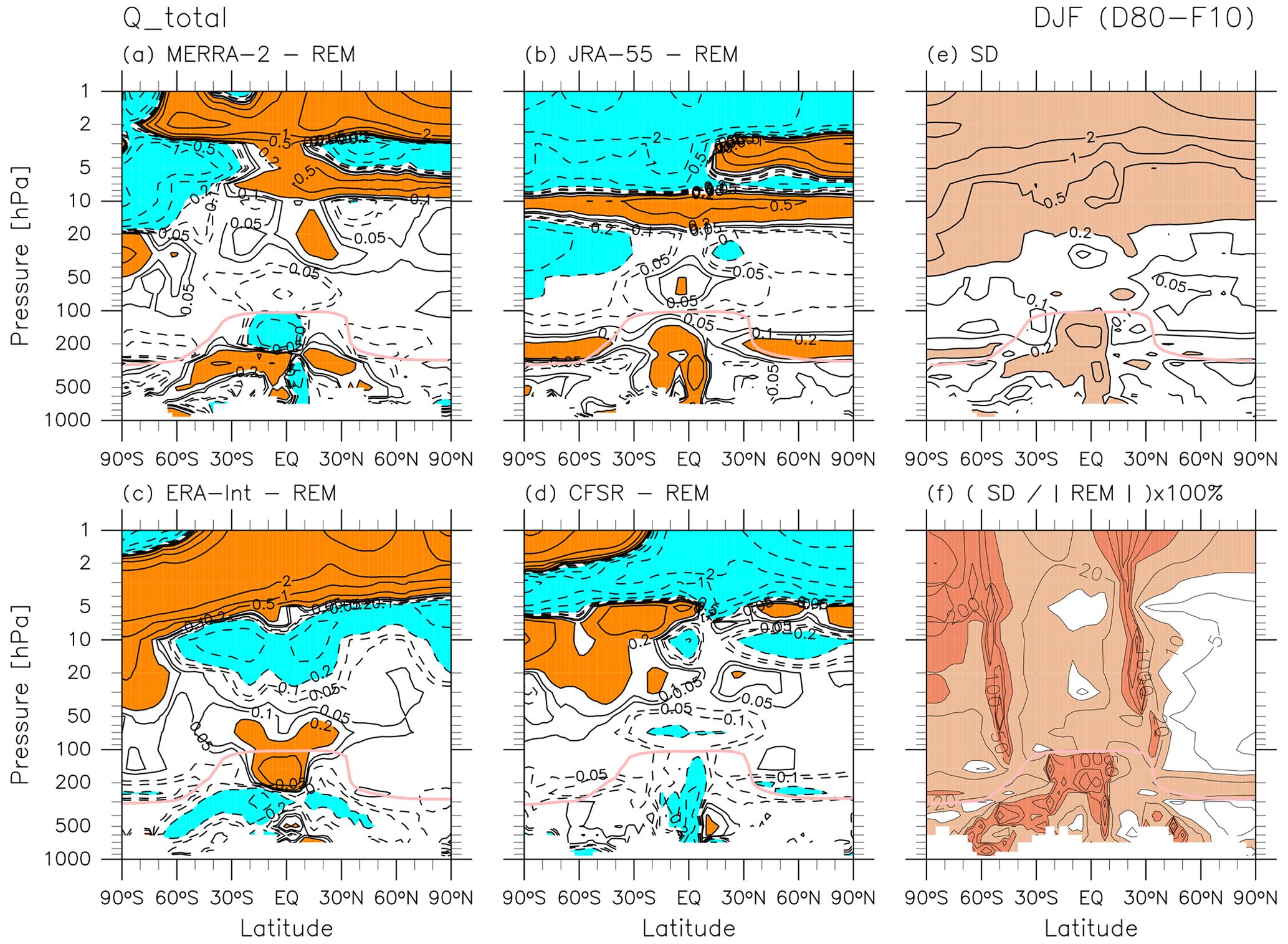
Figure 11 As for Fig. 10, but for the total diabatic heating term of the TEM thermodynamic equation.

Figure 12 As for Fig. 1, but for the 30-year JJA (1981–2010) mean.

Figure 13 As for Fig. 2, but for the 30-year JJA (1981–2010) mean.

Figures 10 and 11 show differences in each reanalysis relative to the REM during DJF for the two major terms of the TEM thermodynamic equation, i.e. the vertical temperature advection term and the total diabatic heating term. The distribution of differences in the vertical temperature advection term reflects inter-reanalysis differences in ${\stackrel{\mathrm{‾}}{\mathit{\omega }}}^{*}$ and ${\stackrel{\mathrm{‾}}{w}}^{*}$ (i.e. vertical bands of positive and negative anomalies, suggesting differences in the structure of the circulation among the reanalyses; Folder 3 in the Supplement) in addition to those in temperature (with greater differences at higher altitudes; Folder 3 in the Supplement). Figure 10f shows that fractional inter-reanalysis differences for the vertical temperature advection term are generally less than 50 % in locations where the term has absolute values greater than 1 K d⁻¹ in the REM (Fig. 4c). This result is consistent with the findings of Abalos et al. (2015), who showed ∼40 % uncertainty in tropical upwelling magnitude. In the NH mid-latitude stratosphere, fractional differences are generally even less than 10 %. Figure 11 shows that differences in the total diabatic heating term show horizontal bands of large positive and negative anomalies in the middle-to-upper stratosphere and large values in the troposphere; these come from combined inter-reanalysis differences in both LW and SW heating (Figs. 8 and 9, respectively). In the upper stratosphere, for the case of CFSR, overestimation of LW cooling is greater than that of SW warming, contributing to a negative total heating difference. ERA-Interim shows the opposite, with overestimation of SW warming exceeding that of LW cooling, resulting in a positive total heating difference. In contrast, for JRA-55, underestimation of LW cooling is less than that of SW warming, leading to a negative total heating difference, while MERRA-2 shows the opposite, leading to a positive total heating difference. Due to the complexity of all these factors, distributions of differences in the two major terms of the TEM thermodynamic equation do not correspond well to each other. Figure 11f shows that fractional inter-reanalysis differences in the SH net heating region (see Fig. 4e) are generally less than 50 %, while those in the NH net cooling region are generally less than 10 %.

The results presented in this section demonstrate that modern global reanalysis systems still need to improve momentum and thermodynamic balance in the middle atmosphere even on the climatological zonal mean scale.

Figure 14 As for Fig. 3, but for the 30-year JJA (1981–2010) mean.

Figure 15 As for Fig. 4, but for the 30-year JJA (1981–2010) mean.

Figure 16 As for Fig. 5, but for the 30-year JJA (1981–2010) mean.

3.2 JJA

3.2.1 REM for JJA

Figure 12 shows the REM climatological latitude–pressure distributions of the TEM variables for JJA. During this season, the SH polar lower stratosphere becomes quite cold and the NH upper stratosphere is warmer than the SH upper stratosphere. As during other seasons, the distributions of temperature and zonal wind agree well with the thermal wind balance in the zonal mean (not shown directly). The BD circulation during this season shows one cell covering the SH and the tropics in the middle-to-upper stratosphere (i.e. the upper branch) and two cells in the lower stratosphere and around the tropopause (i.e. the shallow branches) as observable in both (${\stackrel{\mathrm{‾}}{v}}^{*}$, ${\stackrel{\mathrm{‾}}{w}}^{*}$) and mass streamfunction. As during DJF, the tropical upwelling during this season also has two maxima in the NH and SH subtropics and a minimum in the equatorial lower stratosphere, with the NH subtropical upwelling being much stronger during JJA (in other words, the summer-side tropical upwelling is stronger). We also see the upper-tropospheric branch of the Hadley cells in the tropics, with the tropical-to-SH (anticlockwise) cell being stronger during JJA (thus the winter-side cell is always stronger; see also Fig. 1 and e.g. Schneider and Bordoni, 2008). Northward flow around the SH mid-latitude tropopause is evident in all four reanalyses (see Folder 2 in the Supplement) and is associated with EP flux divergence due to resolved waves there (see Fig. 13 and Birner et al., 2013).

Figure 12 also compares ${\stackrel{\mathrm{‾}}{w}}^{*}$ and ${\stackrel{\mathrm{‾}}{w}}_{{\stackrel{\mathrm{‾}}{v}}^{*}}^{*}$ during JJA. Agreement between the two is weaker than that for DJF (Fig. 1), with more evident differences in the lower stratosphere. As in Fig. 1, comparison of the two mass streamfunctions during JJA in Fig. 12 indicates quantitative differences not only in the upper stratosphere but also in the lower stratosphere.

Figure 13 shows the REM climatological distributions of all terms in the TEM momentum equation for JJA. As for DJF (Fig. 2), the major terms in the stratosphere at monthly timescales are the Coriolis term and the EP flux divergence term but with strong signals extending much higher in the SH than in the NH during JJA because of the existence of the polar night jet in the SH. There are positive signals in EP flux divergence (due to resolved waves) in the SH polar upper stratosphere that are not well balanced with the Coriolis term but are rather balanced by the residual term $\stackrel{\mathrm{‾}}{{\mathit{\epsilon }}_u}$, part of which is due to unresolved forcing from gravity waves. This signature is found in all four reanalyses (see Folder 2 in the Supplement). This pattern may correspond to results from a high-top, high-resolution model analysed by Watanabe et al. (2008, their Fig. 9), who showed strong EP flux convergence due to gravity waves and EP flux divergence due to planetary waves at high altitudes in the high-latitude SH region for July. Around the SH mid-latitude tropopause, signals in the EP flux divergence due to resolved waves correspond to northward flow (see Figs. 12d, 13b, and 13e; Birner et al., 2013). Finally, negative signals in $\stackrel{\mathrm{‾}}{{\mathit{\epsilon }}_u}$ in the mid-latitude lower stratosphere in both hemispheres, as also found for DJF (Fig. 2f), may result in part from unresolved forcing due to gravity waves generated by the subtropical jets (e.g. Kawatani et al., 2004; Plougonven and Snyder, 2007) and the orography (Kuchar et al., 2020). As for DJF, the analysis of zonal acceleration due to parameterizations is provided in Folder 4 in the Supplement. See also Podglajen et al. (2020) for a comparison of reanalyses with long-duration balloon observations.

Figure 14 shows REM climatological distributions of diabatic heating for JJA. In the stratosphere, the distribution of total solar irradiance at the TOA results in distributions of total and radiative heating that are roughly in a mirror image across the Equator to those for DJF (Fig. 3) (e.g. Liou, 2002). The total (and net radiative) diabatic heating is positive in the tropical and mid-latitude stratosphere and strongly negative at high altitudes in the high-latitude SH.

Figure 17 As for Fig. 6, but for the 30-year JJA (1981–2010) mean.

Figure 15 shows REM climatological distributions of all terms in the TEM thermodynamic equation during JJA. As for DJF (Fig. 4), the major terms in the stratosphere at monthly timescales are the vertical advection term and the total (mainly radiative) diabatic heating term, but other terms show noticeable contributions at higher latitudes in the middle-to-upper stratosphere. Furthermore, values of the residual term $\stackrel{\mathrm{‾}}{{\mathit{\epsilon }}_{\mathit{\theta }}}$ are on the same order of magnitude as those for the two major terms in the upper stratosphere, indicating that large differences between the assimilated state and forecast model in this part of the atmosphere also extend to JJA.

Figure 18 As for Fig 7, but for the 30-year JJA (1981–2010) mean.

3.2.2 Differences in each reanalysis from the REM for JJA

The main characteristics of differences in temperature and zonal wind during JJA are similar to those during DJF. Namely, for temperature, the differences among different reanalyses become larger at higher altitudes, and for zonal wind the differences are largest in the tropics and in the low-to-mid-latitude upper stratosphere (Folder 3 in the Supplement). Figure 16 shows differences for ${\mathrm{\Psi }}_{{\stackrel{\mathrm{‾}}{v}}^{*}}^{*}$ during JJA. In the lower stratosphere below the 10 hPa level, the main (SH) cell of the BD circulation (Fig. 12g) is overall stronger for JRA-55 and weaker for MERRA-2 and ERA-Interim (see also differences in ${\stackrel{\mathrm{‾}}{v}}^{*}$ in Folder 3 in the Supplement). Inter-reanalysis standard deviations relative to the REM (Fig. 16f) indicate fractional differences of 5 %–50 % (larger than those for DJF) among these reanalyses in the main (SH) cell of the BD circulation. The features for ${\mathrm{\Psi }}_{{\stackrel{\mathrm{‾}}{v}}^{*}}^{*}$ described above are again generally in agreement with those for ${\mathrm{\Psi }}_{{\stackrel{\mathrm{‾}}{\mathit{\omega }}}^{*}}^{*}$ (Folder 3 in the Supplement).

Figure 19 As for Fig. 8, but for the 30-year JJA (1981–2010) mean.

Figure 20 As for Fig. 9, but for the 30-year JJA (1981–2010) mean.

Figures 17 and 18 show differences in each reanalysis relative to the REM during JJA for the two major terms of the TEM momentum equation (see also Chapter 5 of SPARC, 2022, their Fig. 5.4). Differences in the Coriolis term (Fig. 17) reflect differences in ${\stackrel{\mathrm{‾}}{v}}^{*}$ (Folder 3 in the Supplement). In the mid-latitude lower stratosphere below the 10 hPa level, JRA-55 shows generally positive differences (stronger poleward flows) and MERRA-2 shows generally negative differences (weaker poleward flow), similar to the differences identified for DJF (Fig. 6). Figure 17f shows that fractional differences among the reanalyses for $f{\stackrel{\mathrm{‾}}{v}}^{*}$ are generally less than 50 % (larger than those for DJF) in the SH extratropical stratosphere and NH lower stratosphere, where strong poleward flows are found in the REM (Fig. 12d). In the winter hemisphere, where we expect wave-driven ${\stackrel{\mathrm{‾}}{v}}^{*}$, Fig. 18 shows generally negative differences in the EP flux divergence term (more convergence) in JRA-55 but more mixed results in other reanalyses compared to the DJF case. Large differences in the EP flux divergence term are found in the SH middle-to-upper stratosphere and in the extratropical lower stratosphere in both hemispheres, indicating differences in Rossby and synoptic-scale wave activity across the four reanalyses. As discussed for DJF, it is possible that the differences in the residual term may play a role in the differences in the resolved wave activity but that the interaction between the resolved and unresolved drag differs slightly from that which occurs in the NH during DJF (Cohen et al., 2013; Eichinger et al., 2020; Hájková and Šácha, 2024). Inter-reanalysis fractional standard deviations are generally less than 50 % in the extratropical stratosphere and less than 10 % in the mid-latitude lower-to-middle stratosphere (Fig. 18f); these numbers are again larger than those for the DJF case. Note also the complexity of the anomaly patterns shown in Fig. 18.

Figure 21 As for Fig. 10, but for the 30-year JJA (1981–2010) mean.

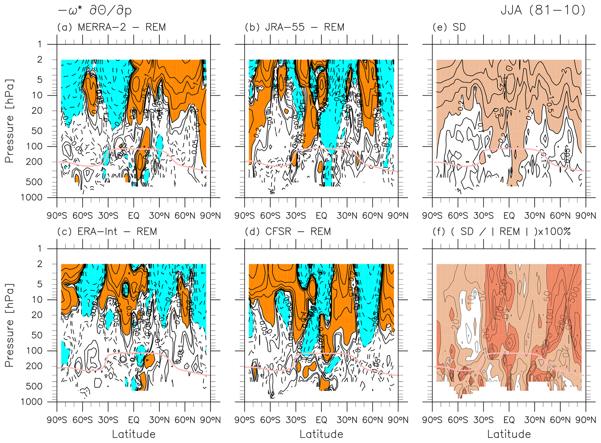
Figure 19 shows differences in LW radiative heating during JJA. The difference patterns are broadly similar to those for DJF (Fig. 8), with the greatest absolute differences again found in the upper stratosphere (fractional differences of 5 %–10 % generally and >10 % in the winter polar stratosphere). Overall, LW heating in MERRA-2 and JRA-55 are more positive than the REM, and ERA-Interim and CFSR are more negative. Furthermore, strong negative differences in CFSR and strong positive differences in JRA-55 are again consistent with the temperature differences in these two reanalyses, i.e. warmer in CFSR and colder in JRA-55 (Folder 3 in the Supplement; Chapter 3 of SPARC, 2022). Thus, the LW heating differences in the upper stratosphere shown in Fig. 19 may be, as for DJF (Fig. 8), largely determined by differences in temperature. As for DJF (Fig. 8f), large fractional differences in LW heating (>10 %) are found around the tropopause globally and in the tropical-to-subtropical lower stratosphere (Fig. 19f), where LW absorption by O₃ is important.

Figure 20 shows differences in SW radiative heating during JJA. Again, as for DJF, the greatest absolute differences are found in the sunlit region of the upper stratosphere (fractional differences of 5 %–10 %), and the strong negative differences in JRA-55 are consistent with negative differences in ozone concentration in this reanalysis (Folder 3 in the Supplement; Chapter 4 of SPARC, 2022). By contrast, differences in ozone distributions cannot fully explain the anomalies in CFSR and MERRA-2. Differences in the tropical upper troposphere during JJA are quite similar for both LW and SW heating to those during DJF and may again be related to differences in the cloud distribution (Wright et al., 2020; Chapter 8 of SPARC, 2022).

Figures 21 and 22 show differences in each reanalysis relative to the REM for the two major terms of the TEM thermodynamic equation during JJA. As for the DJF case, differences in the vertical temperature advection term (Fig. 21) reflect inter-reanalysis differences in ${\stackrel{\mathrm{‾}}{\mathit{\omega }}}^{*}$ and ${\stackrel{\mathrm{‾}}{w}}^{*}$ (i.e. vertical bands of anomalies; Folder 3 in the Supplement) in addition to those in temperature (with greater differences at higher latitudes; Folder 3 in the Supplement). Differences in the total diabatic heating term (Fig. 22) reflect the features in both LW and SW heating (Figs. 19 and 20, respectively) so that the difference patterns in the two major terms of the TEM thermodynamic equation do not correspond well to each other. Fractional inter-reanalysis differences for both (Figs. 21f and 22f) are generally less than 50 % in regions where these terms have large positive or large negative values (Fig. 15), with those in the SH mid-latitude lower-to-middle stratosphere generally less than 10 %.

Again, these results show considerable room for improvement in momentum and thermodynamic balance in modern global reanalysis systems even on the climatological zonal mean scale.

Figure 22 As for Fig. 11, but for the 30-year JJA (1981–2010) mean.

4 Summary

In this paper, the major variables and terms of the TEM momentum and thermodynamic equations were evaluated in the latitude–pressure domain by using four global atmospheric reanalysis datasets, MERRA-2, JRA-55, ERA-Interim, and CFSR, at climatological timescales (1980–2010) in the DJF and JJA seasons (results for MAM and SON have been shown in the Supplement). The characteristics of the REM from these four reanalyses were investigated, along with differences from the REM for each reanalysis. For the REM, variables investigated include residual vertical velocity evaluated from residual meridional velocity through the continuity equation (i.e. using the mass streamfunction), the mass streamfunctions from both residual meridional and vertical velocities, and LW and SW radiative heating. For the TEM equations, the residual terms were also calculated and investigated for their potential usefulness. The residual term for the momentum equation should include the effects of processes parameterized in the reanalysis system such as gravity waves, convective processes, turbulent and numerical diffusion, effects arising from analysis increments, effects associated with using previously interpolated pressure-level data, and errors in the numerical methods (i.e. the evaluation of derivatives). The residual term for the thermodynamic equation should include the effects of analysis increments, defined as differences between the analysis state and the first-guess (forecast) background state in the reanalysis system, as well as effects associated with using pressure-level data and errors in the numerical methods. For differences among different reanalyses, the variables and terms presented in the main text include the mass streamfunction, LW and SW heating, the two major terms of the TEM momentum equation (the Coriolis term and the EP flux divergence term), and the two major terms of the TEM thermodynamic equation (the vertical temperature advection term and the total diabatic heating term).

A comparison between the original residual vertical velocity and the one estimated from residual meridional velocity revealed that the two vertical velocity fields show reasonable agreement in the troposphere and in the lower stratosphere up to 10 hPa, but differences are evident in the upper stratosphere. Because both have their own issues, looking at both estimates of residual vertical velocity and trusting only the common features may be a good approach for studies that need greater accuracy (e.g. those on long-term trends). A comparison between the two mass streamfunctions, one calculated from residual meridional velocity and the other from residual vertical velocity, shows quantitative differences not only in the upper stratosphere (above the 10 hPa level) but also in the lower stratosphere. Estimates of diabatic heating, in particular the LW and SW radiative heating, from modern global atmospheric reanalyses can be considered as the latest “observation-based” (but also highly model-dependent) estimates, against which those from climate models may be evaluated.

The major terms of the TEM momentum equation are the Coriolis term and the EP flux divergence due to waves resolved by the reanalysis grid spacing, which together illustrate the wave-driven stratospheric meridional BD circulation. The residual term of the TEM momentum equation shows interesting signals in the mid-latitude lower stratosphere above the subtropical jets and in the polar upper stratosphere that may result in part from unresolved forcing due to gravity waves generated by the subtropical and polar night jets and the orography. The major terms of the TEM thermodynamic equation are the vertical temperature advection term and the total diabatic heating term in the stratosphere, with the latter almost entirely from radiative heating. Values of the residual term are on the same order of magnitude as those for the two major terms in the middle-to-upper stratosphere, indicating large differences between the observationally constrained analysis and the forecast model at these altitudes.

Differences in each reanalysis from the REM and inter-reanalysis spreads for selected TEM variables and the major terms of TEM momentum and thermodynamic equations were also presented and discussed.

For ${\mathrm{\Psi }}_{{\stackrel{\mathrm{‾}}{v}}^{*}}^{*}$ during DJF, the main NH cell of the BD circulation is generally stronger for JRA-55 and weaker for MERRA-2, with inter-reanalysis fractional differences of 2 %–10 %. For ${\mathrm{\Psi }}_{{\stackrel{\mathrm{‾}}{v}}^{*}}^{*}$ during JJA, the main SH cell of the BD circulation is generally stronger for JRA-55 and weaker for MERRA-2 and ERA-Interim, with inter-reanalysis fractional differences of 5 %–50 %.

The distribution of differences in the Coriolis term reflects that of differences in ${\stackrel{\mathrm{‾}}{v}}^{*}$. During both DJF and JJA, JRA-55 generally shows stronger poleward flows and MERRA-2 generally shows weaker poleward flows in the mid-latitude lower stratosphere, with inter-reanalysis fractional differences of <10 % for DJF and up to 50 % for JJA in the winter extratropical stratosphere and in the summer lower stratosphere, where strong poleward flows are found in the REM. For the EP flux divergence term in the winter hemisphere, where we expect wave-driven ${\stackrel{\mathrm{‾}}{v}}^{*}$, we found differences that correspond qualitatively to those in the Coriolis term, particularly during DJF. Inter-reanalysis fractional differences in the extratropical stratosphere are generally <10 % during DJF and <50 % during JJA.

For LW radiative heating during both DJF and JJA, the greatest absolute differences are found in the upper stratosphere (fractional differences of 5 %–10 % generally and >10 % in the winter polar (upper for DJF) stratosphere), with MERRA-2 and JRA-55 being more positive and ERA-Interim and CFSR being more negative. These differences appear to be largely determined by differences in temperature. Also, during both seasons, large fractional differences (10 %–50 % and even greater in some regions in particular seasons) are found around the tropopause globally and in the tropical-to-subtropical lower stratosphere where heating due to O₃ absorption of upwelling LW radiation fluxes from the troposphere is influential. For SW radiative heating during both seasons, the greatest absolute differences are found in the sunlit region of the upper stratosphere (fractional differences of 5 %–10 %) and the greatest fractional differences are found in the tropical upper troposphere (>50 %) and around the extratropical tropopause (10 %–50 %).

For the two major terms of the TEM thermodynamic equation, differences in the vertical temperature advection term during both seasons reflect those in ${\stackrel{\mathrm{‾}}{\mathit{\omega }}}^{*}$ and ${\stackrel{\mathrm{‾}}{w}}^{*}$ (i.e. vertical bands of anomalies) in addition to those in temperature (with greater differences at higher altitudes), while differences in the total diabatic heating term reflect the combined differences in LW and SW heating. The net result is that the difference patterns in these two terms do not correspond well to each other. Fractional inter-reanalysis differences for both terms during both seasons are generally <50 % in regions where these terms have large positive or large negative values, while those in the winter mid-latitude lower-to-middle stratosphere are generally less than 10 %.

The results for these differences in each reanalysis from the REM and inter-reanalysis spreads illustrate the need for modern global reanalysis systems to further improve momentum and thermodynamic balance even on the climatological zonal mean scale.

The results shown in this paper provide fundamental information on the quality of recent global atmospheric reanalyses in the stratosphere and upper troposphere in the zonal mean TEM framework. Our analysis indicates that the calculated residual term of the TEM momentum equation can be useful to investigate the role of gravity waves in the stratosphere if the impact of gravity waves exceeds the impact of assimilation increments in the momentum balance. Note that the role of gravity waves for the zonal momentum budget is expected to be more accurately constrained in more recent reanalyses, which have higher resolutions and resolve more of the gravity wave spectrum (e.g. Li et al., 2023; Gupta et al., 2021). The calculated residual term in the TEM thermodynamic equation can likewise be useful to investigate analysis increments, highlighting regions and possibly processes where the forecast models need further improvement.