Identifying decadal trends in deweathered concentrations of criteria air pollutants in Canadian urban atmospheres with machine learning approaches

This study investigates long-term trends of criteria air pollutants, including NO₂, CO, SO₂, O₃ and PM_2.5, and O_x (meaning NO₂+O₃) measured in 10 Canadian cities during the last 2 to 3 decades. We also investigated associated driving forces in terms of emission reductions, perturbations due to varying weather conditions and large-scale wildfires, as well as changes in O₃ sources and sinks. Two machine learning methods, the random forest algorithm and boosted regression trees, were used to extract deweathered mixing ratios (or mass concentrations) of the pollutants. The Mann–Kendall trend test of the deweathered and original annual average concentrations of the pollutants showed that, on the timescale of 20 years or longer, perturbation due to varying weather conditions on the decadal trends of the pollutants are minimal (within ±2 %) in about 70 % of the studied cases, although it might be larger (but at most 16 %) in the remaining cases. NO₂, CO and SO₂ showed decreasing trends in the last 2 to 3 decades in all the cities except CO in Montréal. O₃ showed increasing trends in all the cities except Halifax, mainly due to weakened titration reaction between O₃ and NO. O_x, however, showed decreasing trends in all the cities except Victoria, because the increase in O₃ is much less than the decrease in NO₂. In three of the five eastern Canadian cities, emission reductions dominated the decreasing trends in PM_2.5, but no significant trends in PM_2.5 were observed in the other two cites. In the five western Canadian cities, increasing or no significant trends in PM_2.5 were observed, likely due to unpredictable large-scale wildfires overwhelming or balancing the impacts of emission reductions on PM_2.5. In addition, despite improving air quality during the last 2 decades in most cities, an air quality health index of above 10 (representing a very high risk condition) still occasionally occurred after 2010 in western Canadian cities because of the increased large-scale wildfires.

1 Introduction

Criteria air pollutants can harm human health and the natural environment. According to Health Impacts of Air Pollution in Canada 2021 report (Health Canada, 2021), it is estimated that air pollution of NO₂, O₃ and PM_2.5 caused 15 300 deaths per year, corresponding to 42 deaths per 100 000 population in Canada in 2016. To protect human health and the environment, the Canadian Council of Ministers of the Environment (CCME) developed the Canadian Ambient Air Quality Standards (CAAQS) for PM_2.5, O₃, SO₂ and NO₂. CAAQS are supported by four color-coded management levels with each management level being determined by the amount of a pollutant within an air zone, from which recommendations on air quality management actions are provided. Following this standard, multiphase mitigation measures have been implemented to largely reduce anthropogenic air pollutant emissions in recent decades (ECCC, 2023a). Air quality in Canadian urban atmospheres meets CAAQS very well in recent years, as reported in Air Quality Canadian Environmental Sustainability Indictors (ECCC, 2023b).

Nevertheless, the World Health Organization (WHO, 2021) updated the global air quality guidelines (AQG) on NO₂, SO₂, CO, O₃ and PM_2.5 in 2021, based on accumulated strong evidence that air pollution can affect public health even at very low concentrations. In the WHO 2021 AQG, NO₂ annual average concentration is set as 10 µg m⁻³, equivalent to ∼5 ppb at annual average temperatures of 6–10 °C across Canada; annual average and 24 h average PM_2.5 concentrations are set as 5 and 15 µg m⁻³, respectively; and peak season mean 8 h O₃ concentration is set as 60 µg m⁻³. An urgent issue for all areas of the world is to overcome challenges to further lower ambient NO₂, O₃ and PM_2.5 concentrations in order to meet the WHO 2021 AQG (Dabek-Zlotorzynska et al., 2019; Griffin et al., 2020; Xu et al., 2019; Jeong et al., 2020; Al-Abadleh et al., 2021; Wang et al., 2021; Zhang et al., 2022; Bowdalo et al., 2022).

In search of the most efficient mitigation measures for criteria pollutants, the effectiveness of existing measures on air pollution reduction needs to be first examined. For this purpose, long-term trends in concentrations of the criteria air pollutants need to be quantified, and the driving forces of the trends, besides anthropogenic emission reductions, should be identified. Several studies have investigated the decadal trends of some criteria pollutants in Canada in the past decade. For example, Chan and Vet (2010) reported upward trends in O₃ mixing ratio from 1997–2006 at dozens of sites in Canada. Xu et al. (2019) and Zhang et al. (2022) also found increasing trends in O₃ mixing ratio from 1996–2016 at multiple sites in Windsor, Ontario, which was attributed to the reduced titration effect of NO with O₃. They also reported that the 95th percentile O₃ mixing ratio exhibited a decreasing trend and attributed the decrease to anthropogenic emission reductions. Mitchell et al. (2021) reported that the 99th percentile O₃ mixing ratios exhibited a decreasing trend from 2000–2018 at urban and regional sites in Nova Scotia, but such a trend was not found for low-to-moderate percentile O₃ mixing ratios. Bari and Kindzierski (2016) found no significant trends in PM_2.5 mass concentration, although they did find decreasing trends in organic carbon and elemental carbon from 2007–2014 in Edmonton. Jeong et al. (2020) reported a 34 % decrease in PM_2.5 mass concentration from 2004–2017 in Toronto and attributed the decrease to the reduced coal-fired power plant emissions. Wang et al. (2022a) reported significant decreasing trends in organic and elemental carbon in PM_2.5 from 2003–2019 at seven urban sites in Canada. Studies on other criteria pollutants are very limited (Feng et al., 2020; Jeong et al., 2020).

O₃ mixing ratios, especially at high levels, are strongly affected by meteorological conditions; thus, trends on the decadal scale can be perturbed by varying weather conditions from year to year (Simon et al., 2015; Xing et al., 2015; Ma et al., 2021; Lin et al., 2022). Interannual variations of weather conditions also have a strong impact on the decadal trends of other criteria pollutants (Lin et al., 2022). Air quality models are useful tools to analyze emission-driven air quality trends and meteorological impacts (Foley et al., 2015; Astitha et al., 2017; Vu et al., 2019), but most modeling results suffer from large uncertainties which could exceed changes in annual means of simulated pollutant concentrations. Machine learning techniques such as the random forest (RF) algorithm and boosted regression trees (BRTs) have been demonstrated to be powerful tools to decouple impacts of emission changes and perturbations from varying weather and/or meteorological conditions, enabling the derivation of deweathered trends in air pollutant concentrations (Grange et al., 2018; Grange and Carslaw, 2019; Ma et al., 2021; Mallet, 2021; Shi and Brasseur, 2020; Wang et al., 2020; Munir et al., 2021; Lovric et al., 2021; Lin et al., 2022). The advantages and limitations of the RF algorithm and BRTs have been described in detail in earlier studies (Grange et al., 2018; Grange and Carslaw, 2019). Briefly, the BRT method is fast to train and make predictions but suffers heavily from overfitting, which may result in unreliable predictions. The RF method can control the overfitting but yields a poor prediction for outliers for large percentiles. Thus, using two methods with different strengths and weaknesses, although their predictions are similar in many ways, can constrain methodology uncertainties and better evaluate perturbations due to varying weather conditions than using only one method, as has been demonstrated in our earlier study (Lin et al., 2022).

This study attempts to deduct the perturbations due to varying weather conditions on the observed mixing ratios (or mass concentrations) of some criteria air pollutants in Canada during the past 2 to 3 decades and thereby investigates their emission-driven trends. We used the RF algorithm and BRTs to generate the deweathered mixing ratios (or concentrations) of NO₂, SO₂, CO, O₃, O_x and PM_2.5 during the past decades in 10 cities equally distributed in eastern and western Canada. Considering that the machine learning methods may suffer from a weakness in accurately predicting large percentile concentrations of the studied criteria air pollutants, we also applied our previously developed identical-percentile autocorrelation analysis method to better quantify the perturbations due to extreme events such as large-scale wildfires on large percentile PM_2.5 concentrations (Yao and Zhang, 2020; Lin et al., 2022). The Mann–Kendall (M–K) trend test was then employed to resolve the trends in the deweathered mixing ratios (or mass concentrations). Pearson correlation analysis was further conducted for the deweathered and original mixing ratios (or mass concentrations) of the air pollutants against the corresponding provincial-level emissions. City-level emissions were used in the analysis in cases with large differences between air pollutant concentrations and provincial-level emissions. In addition, the Air Quality Heath Index (AQHI, https://weather.gc.ca/airquality/pages/index_e.html, last access: 2 July 2024), a health protection tool designed in Canada to advise the public to adjust outdoor activities based on air pollution levels, was also analyzed with particular attention to the trends with AQHI being above 7 and 10, respectively. This study provides a thorough assessment of the emission-driven trends in the studied criteria pollutants on the timescale of 2 to 3 decades across Canadian urban atmospheres, knowledge from which is much needed in developing future emission control policies of the concerned pollutants.

2 Methodology

2.1 Monitoring sites and data sources

Ten major cities, including five in eastern Canada (Halifax, Québec, Montréal, Toronto and Hamilton) and five in western Canada (Winnipeg, Calgary, Edmonton, Vancouver and Victoria), from the National Air Pollution Surveillance (NAPS) program are selected for investigating decadal trends of the monitored criteria pollutants (Table S1 in the Supplement). The NAPS program has long-term air quality data of a uniform standard across Canada (Dabek-Zlotorzynska et al., 2011, 2019; Jeong et al., 2020; Yao and Zhang, 2020; Wang et al., 2021, 2022a). The NAPS program includes both continuous and time-integrated measurements of gaseous and particulate air pollutants. Continuous data are available as hourly concentrations and are quality-assured as specified in the Ambient Air Monitoring and Quality Assurance/Quality Control Guidelines (https://open.canada.ca/data/en/dataset/1b36a356-defd-4813-acea-47bc3abd859b, last access: 2 July 2024).

Multiple monitoring sites exist in most cities, but only one urban background site was selected in each city mentioned above based on the following criteria: with the most complete dataset of the five selected criteria pollutants (NO₂, CO, SO₂, O₃ and PM_2.5), with the longest data record, and with valid data in each year (Table S1). In cases with a data gap longer than a year, e.g., in Québec, Halifax and Calgary, data at a nearby urban background site (within 1 km) were then used to fill the gap. If no site within 1 km is available, then the data gap is left unfilled. SO₂, CO, NO_x and PM_2.5 emission data at the provincial level in Canada are obtained from https://www.canada.ca/en/environment-climate-change/services/environmental-indicators/air-pollutant-emissions.html (last access: 2 July 2024). City-level air pollutant emissions from various registered facilities since 2002 were obtained from https://www.canada.ca/en/services/environment/pollution-waste-management/national-pollutant-release-inventory.html (last access: 2 July 2024).

Besides the monitored criteria pollutants described above, AQHI is also calculated in this study at 3 h resolution using the following formula (Stieb et al., 2008; To et al., 2013):

$$\begin{array}{rl}\mathrm{AQHI}& =(\mathrm{100}/\mathrm{10.4})\times \left[\right(e^{\mathrm{0.000537}\times {\mathrm{O}}_{\mathrm{3}}}-\mathrm{1})\\ & +(e^{\mathrm{0.000871}\times {\mathrm{NO}}_{\mathrm{2}}}-\mathrm{1})+(e^{\mathrm{0.000537}\times {\mathrm{PM}}_{\mathrm{2.5}}}-\mathrm{1})],\end{array}$$

in which O₃ and NO₂ represent their respective 3 h average original mixing ratios (in ppb), and PM_2.5 represents its 3 h average original concentration (in µg m⁻³). The calculated AQHI is rounded to the nearest positive integer. AQHI between 1–3 represents excellent air quality that is safe for outdoor activities. Outdoor activities may be reduced at AQHI between 4–6 for certain members of the population with some health issues. AQHI values between 7 and 10 and >10 correspond to high and very high health risk conditions, respectively. Note that four alternative AQHI-Plus amendments have been proposed for wildfire seasons, and the AQHI-Plus values are always larger than the corresponding AQHI values (Yao et al., 2020). One of AQHI-Plus amendments has been implemented in late 2016 in British Columbia. The AQHI-Plus amendments are not used in this study since it is not implemented across the whole of Canada.

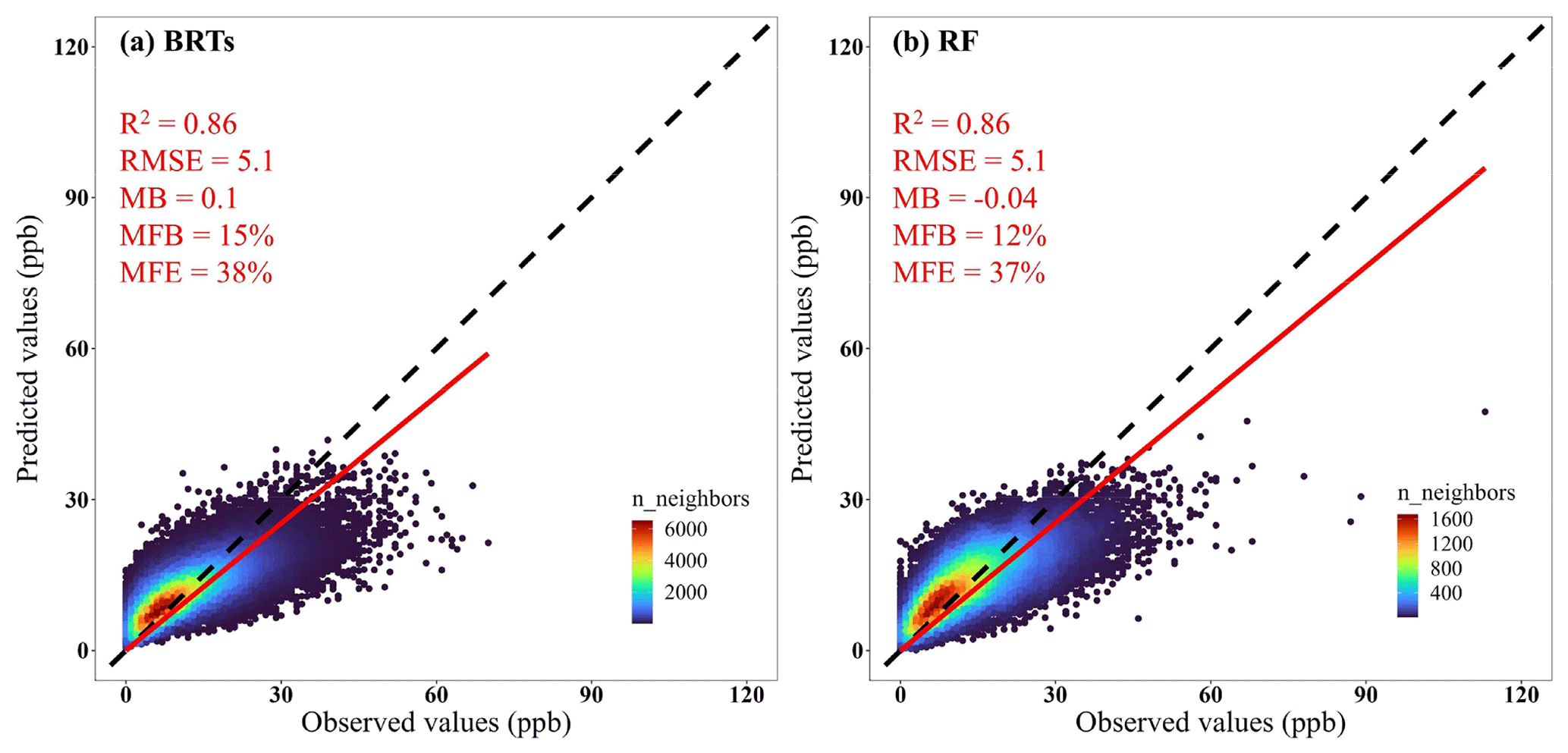
Figure 1 Performance evaluation of the predicted NO₂ hourly mixing ratios by BRTs and the RF algorithm against those observed in Halifax during 1996–2017. Red lines represent linear regression, and the color bar reflects data number density. Note that different observational data sets are shown between (a) and (b) because the inputs for the two packages (BRTs and RF) are randomly divided into two groups for training and testing.

2.2 Statistical analysis

In this study, two popular machine learning packages, including the “rmweather” R package (Grange et al., 2018) and the “deweather” R package (Carslaw and Ropkins, 2012; Carslaw and Taylor, 2009), were used to perform the RF algorithm and the BRTs, respectively. Besides the monitored hourly average mixing ratio (or mass concentration) of a pollutant, temporal variables (hour, day, weekday, week and month) and meteorological parameters (wind speed, wind direction, ambient temperature, relative humidity and dew point) are also needed as additional independent inputs to the machining learning process. The hourly meteorological data were obtained from the meteorological observational station at a nearby airport in each city, which are accessible from the NOAA Integrated Surface Database (ISD) by using the “worldmet” R package (Carslaw, 2021). The meteorological data from the nearest airport in every city should reflect synoptic weather conditions, which have been used in existing machine learning studies (Vu et al., 2019; Mallet, 2021; Wang et al., 2020; Dai et al., 2021; Ma et al., 2021). Additional meteorological parameters such as boundary layer height, total cloud cover, surface net solar radiation, surface pressure, total precipitation and air mass clusters have also been used in some studies to improve the performance of the machine learning methods (Hou et al., 2022; Shi et al., 2021; Lin et al., 2022). These additional meteorological parameters were not included in the present study but could be included in future analyses. Nevertheless, good performance can still be achieved in the present study mainly because of the multi-decade length of the datasets, as demonstrated by an example shown in Fig. 1. Note that the inputs for the two packages were randomly divided into two groups, and the user cannot control the division, i.e., the training dataset that used 80 % of the data and a testing dataset that used the remaining 20 %. Thus, the testing datasets were different between the RF algorithm and the BRTs. Note that all input parameters and output variables, i.e., the predicted hourly average mixing ratio (or mass concentration) of a pollutant, for testing were the same as those used for learning. Moreover, the training and testing were conducted for every pollutant at every site.

Five statistical metrics, including coefficient of determination (R²), root mean square error (RMSE), mean bias (MB), mean fractional bias (MFB) and mean fractional error (MFE), were calculated to evaluate the performance of the two machine learning methods. In the literature, criteria and goal values have not been set for the statistical metrics for the purpose of evaluating machine learning prediction performance. Alternatively, the criteria and goal values for MFE and MFB proposed by the United States Environmental Protection Agency (US EPA) are adopted here, which are MFE ≤75 % and MFB $\le \pm \mathrm{60}\mathit{\%}$ for the criteria value and MFE ≤50 % and MFB $\le \pm \mathrm{30}\mathit{\%}$ for the goal value (US EPA, 2007).

Figure 1 shows predictions against observations of NO₂ mixing ratio in Halifax using the testing datasets during 1996–2017, as an example for evaluating the performance of the two machine learning methods (P value <0.01 for all the correlation). MFB and MFE values were far below their respective goal values for both RF algorithm and BRTs set by US EPA. R² and RMSE were 0.86 and 5.1, respectively, for both methods. MB is −0.04 for RF algorithm and 0.1 for BRTs. The values of these metrics indicated that the predictions reproduced the observations well. However, the two machine learning methods overall underpredicted NO₂ mixing ratios to a small extent based on the regression lines slightly below the 1:1 line. The underestimation was mainly due to sporadic, large values in the measurement of NO₂ mixing ratio, which did not provide sufficient samples for the machine learning methods to learn and yield good predictions. For all the pollutants in all the cities investigated in this study, the machine learning predictions generally met the goal values set by the US EPA, except for PM_2.5 in some western Canadian cities such as Calgary and Edmonton with the predictions only meeting criteria values because of the perturbation from large-scale wildfires.

Following the approach described in earlier studies (Hou et al., 2022; Lin et al., 2022), the two machine learning methods were run for 1000 times with meteorological variables randomly resampled from the entire datasets during the study period. The average model prediction from the 1000 model runs represents the meteorologically normalized pollutant concentration at a particular time. We also tested averaging 2000 and 3000 model predictions, which produced consistent results with those of using 1000 model predictions. Thus, averaging 1000 model predictions was used for meteorological normalization in this study.

As mentioned above, the machine learning methods suffer from a weakness in accurately predicting high concentration values for large percentiles. We thus applied the identical-percentile autocorrelation analysis method developed in our previous study to quantify the perturbations due to extreme events such as large-scale wildfires on the large percentile concentration values (Yao and Zhang, 2020; Lin et al., 2022). This method has five steps for data processing and analysis. The first step is to construct a long-term average data series at hourly resolution covering 365 d by averaging the corresponding hourly data from all the years of the study period. The second step is to pair a data series at any given year to the long-term average data series, and if there were any data gaps (missing hours) in the former data series, data for these hours in the latter series were also removed so that the two data series have exactly the same size. The third step is to rearrange all the hourly data from the smallest to the largest value in each of the data series generated in step 2 and then conduct correlation analysis between the pair of data series. Inflection points in the large and small percentile zone were first visibly identified/guessed and referenced as upper and lower inflection points, respectively. The pair of data between the lower and upper inflection points were correlated repeatedly by varying values of the two inflection points in search of the highest R² values. The fourth step is to predict the large percentile values exceeding the upper inflection point using the regression equation with the highest R² generated in step 3. The final step is to obtain the perturbations due to extreme events on the large percentile concentrations by subtracting the observed values from the predicted values.

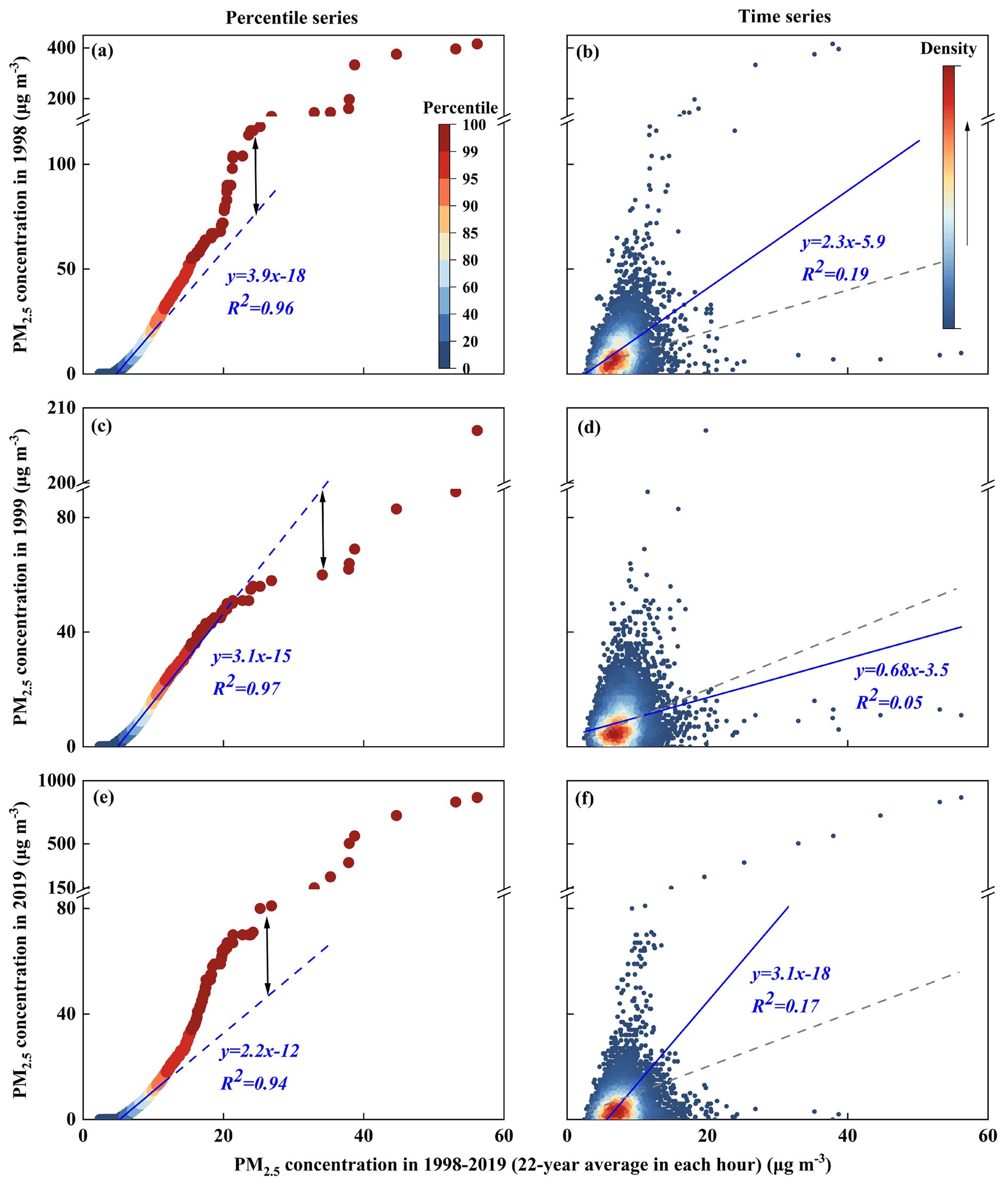
Figure 2 Correlations between hourly PM_2.5 concentration in a single year and 22-year average PM_2.5 concentration in each hour of the year in Edmonton. Panels (a), (c), and (e) show percentile series of PM_2.5 in 1998, 1999, and 2019, respectively, against the corresponding 22-year average series. Panels (b), (d), and (f) show time series of PM_2.5 in 1998, 1999, and 2019, respectively, against the corresponding 22-year average series. Blue straight dashed lines in (a), (c) and (e) represent the regression curves within linear ranges and their extensions out of the ranges; vertical arrows represent the distance between the predicted values from the regression curve. Blue straight lines and dark blue dashed lines in (b), (d) and (f) represent the regression curves and 1:1 lines, respectively.

Figure 2 shows three examples calculating the perturbations due to varying weather conditions and large-scale wildfires on the large percentile concentrations of PM_2.5 in 1998, 1999 and 2019 in Edmonton. Large-scale wildfires occurred in 1998 and 2019 (Fig. S1), but there is no record in 1999. In 1998, data points outside the 4.5th–94th percentile range were screened out through steps 1–3, and the remaining data points were used to obtain a regression equation, which shows [PM_2.5]_{data  in  1998} = [PM_2.5]_{long-term  average} × 3.9–18 (R²=0.96, P<0.01) (Fig. 2a). [PM_2.5]_{data  in  1998} and [PM_2.5]_{long-term  average} represent the same identical percentile values of PM_2.5 in reorganized data series of 1998 and the long-term average through steps 1–3, respectively. The similar definition is applicable for [PM_2.5]_{data  in  1999} and [PM_2.5]_{data  in  2019} presented below. In 1999, data points within the 4.5th–99.7th percentile range resulted in a regression equation of [PM_2.5]_{data  in  1999}= [PM_2.5]_{long-term  average} × 3.1–15 (R²=0.97, P<0.01) (Fig. 2c). In 2019, data points within the 5.4th–96th percentile range resulted in [PM_2.5]_{data  in  2019}= [PM_2.5]_{long-term  average} × 2.2–12 (R²=0.94, P<0.01) (Fig. 2e). Note that step 3 is critical to obtain these excellent correlations (Fig. 2a, c and e) as compared with those without step 3 (Fig. 2b, d and f).

The perturbation due to the extreme weather conditions or the extreme events on the 100th percentile PM_2.5 value, i.e., the maximum value in this study, at a particular year (y) can be calculated as

$$\begin{array}{rl}& [{\mathrm{PM}}_{\mathrm{2.5}}{]}_{\text{perturbation\hspace{0.17em} at\hspace{0.17em} 100th},y}=[{\mathrm{PM}}_{\mathrm{2.5}}{]}_{\text{predicted\hspace{0.17em} at\hspace{0.17em} 100th},y}\\ & -[{\mathrm{PM}}_{\mathrm{2.5}}{]}_{\text{observed\hspace{0.17em}at\hspace{0.17em} 100th},y},\end{array}$$

[PM_2.5]${}_{\text{predicted\hspace{0.17em} at\hspace{0.17em} 100th},y}=$ [PM_2.5]_{long-term  average  at  100th} $\times k_y+b_y$ ,

where [PM_2.5]_{observed  at  100th,y} represents the 100th percentile PM_2.5 value observed in y year, and k_y and b_y represent the slope and intercept, respectively, of the regression equation with the highest R² in the y year generated through steps 1–3. Similarly, the perturbation inherent from the large percentile values from the final upper inflection point (mth) to 100th percentile in a particular year can be calculated as

$$\begin{array}{rl}& [{\mathrm{PM}}_{\mathrm{2.5}}{]}_{\text{perturbation\hspace{0.17em} at}\ge m\mathrm{th},y}=[{\mathrm{PM}}_{\mathrm{2.5}}{]}_{\text{predicted\hspace{0.17em} at}\ge m\mathrm{th},y}\\ & -\left[{\mathrm{PM}}_{\mathrm{2.5}}{]}_{\text{observed\hspace{0.17em} at}\ge m\mathrm{th},y,}\right[{\mathrm{PM}}_{\mathrm{2.5}}{]}_{\text{predicted\hspace{0.17em} at}m\mathrm{th},y}\\ & =[{\mathrm{PM}}_{\mathrm{2.5}}{]}_{\text{long-term\hspace{0.17em} average\hspace{0.17em} at}m\mathrm{th}}\times k_y+b_y.\end{array}$$

The calculated values from [PM_2.5]${}_{\text{perturbation\hspace{0.17em} at}\ge m\mathrm{th},y}$ to [PM_2.5]_{perturbation  at 100th,y} in the y year were averaged as [PM_2.5]_{perturbation  average,y}. The perturbation contribution to the corresponding original annual average equals to [PM_2.5]${}_{\text{perturbation\hspace{0.17em} average},y}\times$ (1 m %) in y year, and the values were 3.0 µg m⁻³ in 1998, 0.2 µg m⁻³ in 1999 and 1.7 µg m⁻³ in 2019 in Edmonton, corresponding to strong, minimal and moderate perturbations, respectively, from large wildfires.

The M–K trend test is a non-parametric test applicable to any type of data distribution and is employed to resolve the trends in the time series of the deweathered and original annual average concentration of each pollutant. Qualitative trends revolved by the M–K trend test include (1) an increasing or decreasing trend with a P value of <0.05 and (2) no significant trend including a probably increasing or decreasing trend, a stable trend, and a no-trend with all the other conditions (Aziz et al., 2003; Kampata et al., 2008; Yao and Zhang, 2020). The extracted trends and associated driving factors are discussed in detail below.

Table 1 Regression of (BRTs and RF) deweathered against original annual average NO₂ mixing ratios, annual decreasing rate (ppb yr⁻¹), and overall decreasing percentage (%) of deweathered and original NO₂ mixing ratios (P<0.05 for all the decreasing trends), with correlation (R²) of deweathered and original NO₂ mixing ratios against provincial total NO_x emissions and transportation NO_x emissions (P<0.05, except those marked with “–” for which p>0.05), as well as percentage decreases (%) of the provincial total NO_x emissions and transportation NO_x emissions (P<0.05 for all the decreasing trends, except increasing trends in NO_x emission from 1990–2010 in Winnipeg and Calgary^a) in 10 Canadian cities during the last decades (^b since 1990; bold font numbers represent cases with smaller deceasing percentages in NO₂ mixing ratios than in corresponding provincial emissions; italic numbers represent R²>0.8; and italic bold numbers represent an increasing trend).

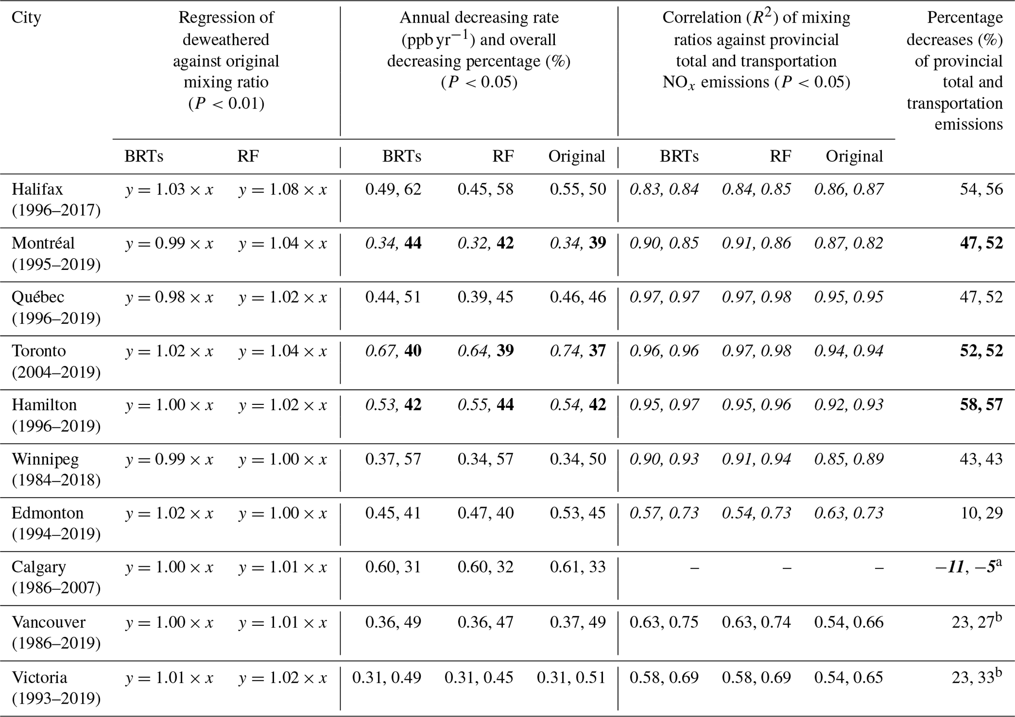
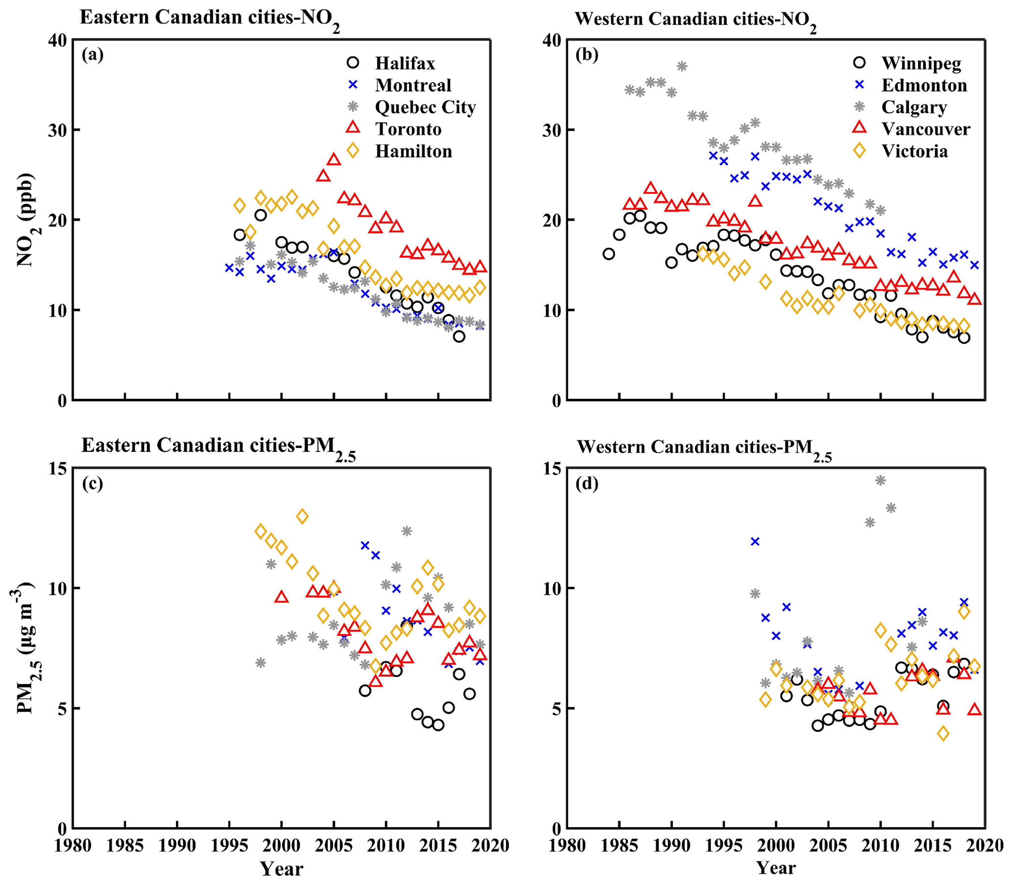
Figure 3 Trends of original annual average NO₂ (a, b) and PM_2.5 (c, d) in five eastern (a, c) and five western (b, d) Canadian cities.

3 Results

3.1 Trends in deweathered and original NO₂ mixing ratios

Figure 3a and b show decadal variations in the original annual averages of NO₂ mixing ratios in the 10 Canadian cities. The BRT-deweathered and RF-deweathered hourly averages of NO₂ mixing ratios are shown in Fig S2, in which the deweathered results were also interpreted in terms of increased or reduced emissions of NO_x. The decadal trends resulted from annual averages of BRT-deweathered, RF-deweathered and original NO₂ mixing ratios are listed in Table 1.

The deweathered and original annual average NO₂ mixing ratios in any of the 10 cities both showed consistent decreasing trends in the last 2–3 decades (P<0.05 through M–K trend test). The BRT-deweathered and RF-deweathered annual averages highly correlated with the original values with R²>0.95 and P<0.01 (Table 1). The slopes of zero-intercept regression equations between the deweathered and original annual average NO₂ mixing ratios were mostly within 0.98–1.04, indicating ≤4 % differences between the deweathered and original annual values. These results indicated that the perturbation due to varying weather conditions only exerted minor influences on the original annual averages. The only exception is the RF-deweathered annual averages in Halifax (with a slope of 1.08); however, this may not suggest that the perturbation due to varying weather conditions was as high as 8 % since the BRT-deweathered annual averages in the same city showed a slope of only 1.03, indicating that the uncertainties in the slope associated with the RF-deweathered averages can be as large as 5 % (8 % minus 3 %) because of its poor prediction for large outlier values.

The annual decreasing rates in the deweathered and original NO₂ mixing ratios in the studied cities varied from 0.31 to 0.74 ppb yr⁻¹, and the overall percentage decreases ranged from 37 % to 62 % during the last 2 to 3 decades (Table 1). Our results suggested that varying weather conditions likely played a negligible role in the annual decreasing rates of NO₂ mixing ratio in two eastern (Montréal and Hamilton) and four western (Winnipeg, Calgary, Vancouver and Victoria) Canadian cities, as can be seen from the very close annual decreasing rates between the deweathered and original annual average mixing ratios, despite methodology uncertainties in generating deweathered mixing ratios as mentioned above. In the remaining four cities, the annual decreasing rates were always larger in the original than the deweathered annual average NO₂ mixing ratio, with the largest differences in Toronto (0.07–0.10 ppb yr⁻¹), followed by Halifax (0.06–0.10 ppb,yr⁻¹), Edmonton (0.06–0.08 ppb yr⁻¹) and Québec (0.02–0.07 ppb yr⁻¹), suggesting that varying weather conditions contributed appreciably to the annual decreasing rate. The annual decreasing rates were highly city-dependent, but there were no significant differences between eastern and western cities (P>0.05). With continuously decreasing NO₂ mixing ratios in the last decades (Fig. 3), annual average NO₂ fell to below 10 ppb by 2019 in half of the studied cities (Halifax, Montréal, Québec, Winnipeg and Victoria), meeting the WHO 2021 guideline. Additional efforts are still needed to lower the NO₂ level in the rest of the cities, especially in Toronto and Edmonton in which annual average NO₂ values were still as high as 15 ppb in 2019.

NO₂ in urban atmospheres was mainly formed by the rapid titration reaction of NO with O₃, with NO largely released from anthropogenic emissions, especially the transport sector (Pappin et al., 2016; Casquero-Vera et al., 2019; Dabek-Zlotorzynska et al., 2019; Feng et al., 2020; Griffin et al., 2020; Al-Abadleh et al., 2021). The correlations between the annual average NO₂ mixing ratios and corresponding provincial NO_x emissions were thereby analyzed below (Table 1). Note that the online air pollutant emission inventory in Canada reports the emissions since 1990 (ECCC, 2021), so the correlation analysis only covers the period of 1990–2019. Strong correlations (R²=0.82–0.98) were obtained in all of the five eastern Canadian cities. The overall decreasing percentages of the deweathered and original NO₂ mixing ratios in Halifax and Québec were roughly the same as those of the provincial grand total NO_x emissions and transportation NO_x emissions, but in Montréal, Toronto and Hamilton the former decreasing percentages were smaller than the latter ones. In contrast, the overall decreasing percentages in NO₂ mixing ratio in the five western Canadian cities were substantially larger than the corresponding decreasing percentages of the provincial grand total NO_x emissions and transportation NO_x emissions, and the correlations (R²=0.54–0.94) between NO₂ mixing ratio and provincial emission were not as good as those in eastern cities. The extreme case occurred in Calgary, where NO₂ mixing ratio decreased by 31 %–33 % during 1990–2007 when the grand total NO_x emissions and transportation NO_x emissions in Alberta increased by 11 % and 5 %, respectively, noting that a much shorter period of data was used in this than other cities. The city-level NO_x emissions recorded from various facilities in Calgary increased from 68 t in 2002 to 262 t in 2007 (Table S2), which cannot explain the decrease in NO₂ mixing ratios.

3.2 Trends in deweathered and original mixing ratios of CO and SO₂

As mentioned earlier, CO and SO₂ in Canadian cities well met the CAAQS in recent years. The original annual average mixing ratios of CO and SO₂ in the 10 cities generally met the WHO 2021 air quality guidelines in the last decade, except SO₂ in Hamilton (Fig. S4). Thus, the analysis results on deweathered and original mixing ratios of SO₂ and CO in the nine cities and CO in Hamilton were only briefly summarized below, leaving SO₂ in Hamilton to be discussed separately.

The annual averages of the deweathered CO mixing ratios were reasonably consistent with the original annual averages in five cities, e.g., the slopes of the deweathered mixing ratios against the original ones varied from 0.97 to 1.03 in Montréal, Hamilton, Winnipeg, Edmonton, Vancouver and Victoria, although somewhat large differences between the deweathered and original mixing rations were seen in Québec with a slope of 1.12 (RF vs. original) and Toronto with a slope of 0.92 (BRTs vs. original). The original and deweathered annual averages of CO decreased by ≥82 % in the last 2 to 3 decades in six cities, including Halifax (90 %–92 %), Calgary (90 %–91 %), Winnipeg (84 %–88 %), Edmonton (86 %–86 %), Toronto (83 %–86 %) and Vancouver (82 %–83 %) (Table S3), followed by 66 %–70 % in Hamilton and less than 60 % in Québec (56 %–58 %) and Victoria (57 %–59 %). Large percentage decreases in baseline CO mixing ratios across North America were reported before (Zhou et al., 2017). The deweathered and original annual averages of CO mixing ratio significantly correlated with the corresponding provincial grand total emissions and transportation emissions of CO (R²=0.68–0.96, P<0.01) in these nine cities. The overall percentage decreases in CO mixing ratio in Québec and Victoria were approximately the same as those in the corresponding provincial transportation emissions of CO; however, the former percentage decreases were evidently larger than the latter ones in the other seven cities mentioned above. In Montréal, no significant trends were obtained in the deweathered and original CO mixing ratios during 1995–2010 (P>0.05), despite the fact that the provincial total CO emissions and transportation CO emissions decreased by 37 % and 53 %, respectively, during the same period.

The deweathered and original annual average mixing ratios of SO₂ decreased by 89 %–97 % in the last 2 to 3 decades in four cities, including Winnipeg (95 %–97 %), Vancouver (90 %–95 %), Toronto (89 %–95 %) and Halifax (90 %–93 %), followed by 79 %–86 % in Montréal, 78 %–85 % in Québec, 73 %–82 % in Victoria, 62 %–64 % in Calgary and 52 %–55 % in Edmonton (Table S4). Large percentage decreases in SO₂ mixing ratio have been reported in rural atmospheres across North America during the last 2 to 3 decades (Xing et al., 2015; Feng et al., 2020). Since 1990, the overall decreasing percentages in SO₂ mixing ratio in Halifax, Toronto, Calgary and Vancouver were evidently larger than those of the corresponding provincial grand total SO₂ emissions. In Montréal, Québec, Winnipeg and Edmonton, the percentage decreases in SO₂ mixing ratio were close to those in the corresponding provincial grand total SO₂ emissions during the same periods. Although SO₂ mixing ratio in Victoria decreased by 73 %–82 % during 1999–2019, the corresponding provincial grand total SO₂ emission did not decrease much during the same period. However, the city-level SO₂ emissions from registered facilities in Victoria decreased from 217 t in 2002 to near zero in 2019 (Table S2), supporting the decreases in SO₂ mixing ratios. Note that the differences between the two deweathered mixing ratios of SO₂ were enlarged to some extent in comparison with other pollutants, e.g., with the differences being 10 %–12 % for SO₂ but only 2 %–5 % for NO₂ (as presented above), in Montréal, Toronto and Winnipeg. The increased uncertainties led to the difference between the RF-deweathered and original SO₂ mixing ratios being up to 16 % in Winnipeg, based on the slope of 1.16 listed in Table  S4. The difference between the BRT-deweathered and original SO₂ mixing ratios was, however, only 4 %, suggesting that the perturbation due to varying weather conditions might be within 4 %–16 %. Again, the RF algorithm suffers from a weakness in predicting large outlier values.

In Hamilton, the annual average of the deweathered SO₂ mixing ratios were highly consistent with those of the original data as indicated by the close to 1.0 slopes. The deweathered and original annual averages of SO₂ mixing ratios decreased by 23 %–28 % during 1996–2019, which were substantially smaller than the 81 % decrease of the corresponding provincial grand total SO₂ emissions during the same period. Such a large discrepancy indicates that the reduction in SO₂ emission in Hamilton likely substantially lagged behind the average provincial level. This is indeed the case since SO₂ emissions from registered facilities in Hamilton (Table S2) fluctuated around $\mathrm{8.67}\pm \mathrm{1.75}\times {\mathrm{10}}^{\mathrm{3}}$ t yr⁻¹ during 2002–2009 and then increased to $\mathrm{1.14}\pm \mathrm{0.13}\times {\mathrm{10}}^{\mathrm{4}}$ t yr⁻¹ during 2010–2018. This also caused the weak correlations between annual average SO₂ mixing ratio in this city and provincial total SO₂ emission (R²=0.42–0.57, P<0.05). In addition, the original annual average SO₂ mixing ratio increased from 3.2–3.5 ppb in 2016–2017 to 4.8–5.0 ppb in 2018–2019 when provincial total SO₂ emission changed little. Thus, reducing local SO₂ emissions in Hamilton is critical to further lower SO₂ mixing ratio in this city in order to meet the CAAQS and the WHO 2021 guideline, despite the existence of other factors such as regional transport (Zhou et al., 2017; Ren et al., 2020).

3.3 Trends in deweathered and original O₃ and O_x mixing ratios

The original annual averages of O₃ and O_x are shown in Fig. S5 and the analysis results of deweathered and original annual averages are listed in Table S5. Increasing trends in the deweathered and original annual average O₃ mixing ratio were obtained in nine cities during the last 2 to 3 decades, with Halifax as an only exception that showed no significant trend (P>0.05) during 2000–2017. Theoretically, the increasing trends in the O₃ mixing ratios could be caused by the enhanced tropospheric photochemical formation of O₃ and/or the weakened titration reaction between O₃ and NO due to the substantial reduction of NO emissions (Simon et al., 2015; Zhou et al., 2017; Sicard et al., 2020; Mitchell et al., 2021; Wang et al., 2022b) (more discussion in Sect. 4.2 below). In contrast, the decreasing trends in the deweathered and original annual average O_x mixing ratios were generally obtained, except in Victoria where there was no significant trend (P>0.05) during 2000–2017. The opposite long-term trends between O₃ and O_x suggested that the increase in O₃ is much less than the decrease in NO₂, which does not support the hypothesis of the enhanced tropospheric formation of O₃.

The deweathered and original annual average O₃ mixing ratios increased by 10 ppb in Edmonton from 1981–2019, 8 ppb in Hamilton from 1996–2019 and Calgary from 1986–2014, and <7 ppb in the other cities (Fig. S5, Table S5). The increased O₃ mixing ratio was likely caused by the reduced titration reaction between O₃ and NO, considering the reduced photochemical formation of O₃ in the troposphere (Simon et al., 2015; Xing et al., 2015). Varying weather conditions likely exerted a negligible influence on the decade increases in O₃ mixing ratio in Edmonton, Hamilton, Calgary and Vancouver on the basis of the almost identical increases in deweathered and original annual averages. However, the comparison between deweathered and original annual averages also showed that varying weather conditions did cause an increase of 2 ppb out of the total of 7 ppb increase in the original annual average O₃ in Winnipeg from 1985–2018, and 1 ppb increase in Montréal from 1997–2010 and in Toronto from 2003–2019. In contrast, varying weather conditions likely caused a 1 ppb decrease in Québec from 1995–2019 and in Victoria from 1999–2019.

The deweathered and original annual average O_x mixing ratios decreased by 10–12 ppb in Vancouver from 1986–2019, 10 ppb in Halifax from 2000–2019 and in Toronto from 2003–2019, 8–10 ppb in Edmonton from 1981–2019, and <6 ppb in the other cities (Fig. S5 and Table S5). Based on the simultaneously monitored NO mixing ratios and the method reportedly used for estimating the primary NO₂ emission (Kurtenbach et al., 2012; Simon et al., 2015; Casquero-Vera et al., 2019; Xu et al., 2019), the reduced primary NO₂ emissions likely accounted for only 1–2 ppb decrease in O_x in the 10 cities and generally acted as a minor contributor to the decrease in O_x.

Table 2 Regression of (BRTs and RF) deweathered against original annual average PM_2.5 mass concentrations, annual decreasing rate (µg m⁻³ yr⁻¹) and overall decrease (µg m⁻³) of deweathered and original PM_2.5 mass concentrations, and percentage decreases (%) of the provincial total PM_2.5 emissions in 10 Canadian cities during the last decades (decreasing trends were obtained with P<0.05 except those marked with “–” for which P>0.05; and bold font numbers represent cases with increasing trends).

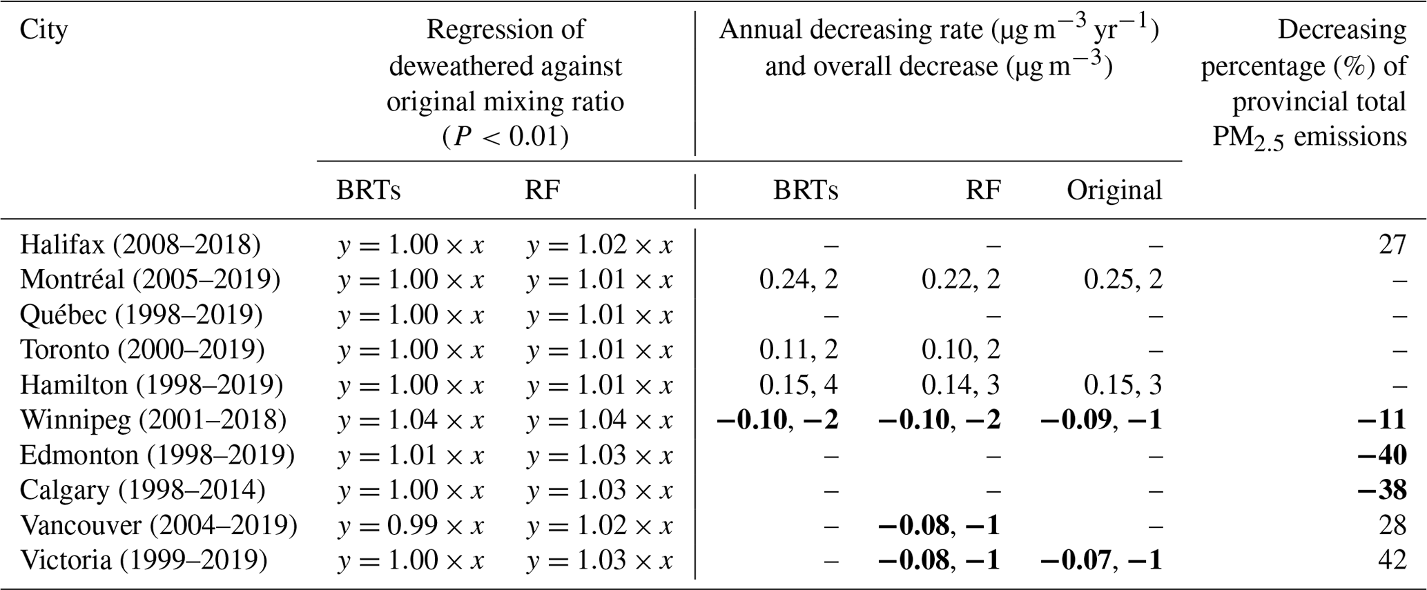
3.4 Trends in deweathered and original PM_2.5 mass concentrations

Opposite decadal trends were observed between eastern and western Canadian cities in the deweathered and original PM_2.5 mass concentrations (Table 2, Figs. 3c and d, and S6). In eastern Canadian cities, either decreasing or no significant trends were obtained in the last 2 decades. The decreasing trends (P<0.05) were identified in the RF-deweathered, BRT-deweathered and original annual average PM_2.5 in Montréal from 2005–2019 and in Hamilton from 1998–2019. The overall decreases were only 2 µg m⁻³ with the decreasing rate of 0.22–0.25 µg m⁻³ yr⁻¹ in Montréal and 3–4 µg m⁻³ and 0.14–0.15 µg m⁻³ yr⁻¹ in Hamilton. The decreasing trends (P<0.05) were also identified in the RF-deweathered and BRT-deweathered PM_2.5 in Toronto from 2000–2019 with an overall decrease of only 2 µg m⁻³ and a decreasing rate of only 0.10–0.11 µg m⁻³ yr⁻¹. However, no significant trend (P>0.05) was identified in the original annual average PM_2.5 in Toronto, implying that the perturbation due to varying weather conditions likely canceled out the mitigation effects of air pollutants. Note that there were no decreasing trends in the provincial total primary PM_2.5 emissions in Quebec and Ontario during the periods when PM_2.5 mass concentration decreased in the three abovementioned cities. This was not surprising, because the major chemical components in PM_2.5 were derived mainly from secondary sources (Dabek-Zlotorzynska et al., 2019; Jeong et al., 2020; Wang et al., 2021). The decreasing provincial emissions of SO₂, NO_x, and volatile organic emissions in Quebec and Ontario likely have reduced the amounts of their oxidized products in PM_2.5 (Xing et al., 2015; Yao and Zhang, 2019, 2020; Feng et al., 2020; Jeong et al., 2020; ECCC, 2021; Wang et al., 2021, 2022a). No significant trends (P>0.05) were identified in the deweathered and original PM_2.5 concentrations in Halifax from 2008–2018 or in Québec from 1998–2019, which need further investigation.

In western Canadian cities, either increasing or no significant trends were extracted in the deweathered and original annual average PM_2.5 mass concentrations. Increasing trends (P<0.05) were identified in the RF-deweathered, BRT-deweathered and original annual average PM_2.5 in Winnipeg from 2001–2018 with an overall increase of only 1–2 µg m⁻³ and an increasing rate of 0.09–0.10 µg m⁻³ yr⁻¹. Increasing trends (P<0.05) were identified in the RF-deweathered and original annual average PM_2.5 in Victoria from 1999–2019 with an overall increase of only 1 µg m⁻³ and an increasing rate of 0.07–0.08 µg m⁻³ yr⁻¹, but no significant trend was identified in the BRT-deweathered annual average PM_2.5. An increasing trend was obtained only in the RF-deweathered annual average PM_2.5 in Vancouver from 2004–2019, and no significant trends were identified in the BRT-deweathered and original annual average PM_2.5. The inconsistency between the trends extracted from the three different annual average PM_2.5 data series was mostly because of the small magnitudes of the actual interannual changes and thus the trends, which are on the same order of magnitude as the methodology uncertainties. Considering the decreasing trends in NO₂, CO and SO₂ mixing ratios discussed above and the reported decreasing trends in secondary chemical components of PM_2.5 in Western Canada (Wang et al., 2021, 2022a), the increasing trends in the deweathered and/or original annual average PM_2.5 observed in some western Canadian cities were likely caused by increased natural emissions, such as from the increased large-scale wildfires in recent years.

It is noticed that a few spikes always appeared in the BRT-deweathered PM_2.5 concentrations in the five western Canadian cities since 2010 (Fig. S6). Most of these spikes were associated with large-scale wildfire emissions (Littell et al., 2009; Collier et al., 2016; Landis et al., 2018; Matz et al., 2020). For example, wildfires caused large and rapid increases in PM_2.5 mass concentration from ≤10 to >400 µg m⁻³ in Edmonton during 10–12 August 1998 and on 30 May 2019 (Fig. S1). During these periods, the BRT method predicts the spikes of PM_2.5. However, the RF method seemingly failed to learn the wildfire signals and missed predicting the spikes associated with largely increased natural emissions because of its inherent weakness.

To further explore the causes for the different trends in PM_2.5 between eastern and western Canadian cities, the 95th–100th percentile PM_2.5 mass concentration data in each year were averaged into annual value and were examined below. The top 5 % PM_2.5 exhibited decreasing trends (P<0.05) in four eastern Canadian cities and no significant trend (P>0.05) in Halifax (Fig. S7). The decreasing trends further confirmed the mitigation effects of air pollutants on PM_2.5. However, annual average PM_2.5 was still as high as 8.8 µg m⁻³ in Hamilton in 2019; 7.0–7.7 µg m⁻³ in Québec, Toronto, and Montréal; and 5.6 µg m⁻³ in Halifax. If keeping the same decreasing rates as mentioned above, it would take another 1 to 3 decades to lower annual average PM_2.5 by 2–4 µg m⁻³ in order to meet the WHO 2021 guideline.

No significant trends (P>0.05) were identified in the 95th–100th percentile PM_2.5 mass concentrations in the five western Canadian cities. Note that a large standard deviation of the 95th–100th percentile PM_2.5 mass concentration was found in some years in the five western cities, indicating a high variability. However, this is not the case in the eastern Canadian cities. The episodic PM_2.5 events likely canceled out the mitigation effects in the western Canadian cities. The annual average PM_2.5 were 6.6–6.8 µg m⁻³ in 2019 in Winnipeg, Edmonton and Victoria, which need great additional mitigation efforts in order to reduce to a level below 5 µg m⁻³ in the presence of the episodes caused by natural emissions. Note that the annual average PM_2.5 was already lower than 5 µg m⁻³ in Vancouver and that the annual average was 8.4 µg m⁻³ at the study site in Calgary in 2014. The value slightly decreased to 7.6 µg m⁻³ in 2019 at another site ∼5 km from the study site in Calgary.

3.5 Trends in AQHI in the 10 Canadian cities

Decreasing trends in AQHI were obtained in nine cities (P<0.05), with Calgary as an only exception (Figs. S9 and S10). The annual average AQHI decreased by 8 %–29 % during the last 2 decades to the levels of 1.8 to 3.0 during 2017–2019 in the nine cities. In Calgary, the annual averages AQHI narrowed around 3.4±0.2 during 1998–2010. In the five eastern cities, AQHI above 10 occurred at <0.3 % frequency before 2010 but none after 2010. AQHI between 7–10 occurred at <4 % frequency before 2010 and below 0.5 % after 2010. In the five western cities, AQHI above 10 occurred at <0.3 % frequency, and AQHI between 7–10 occurred at <2 % frequency during the last 2 decades. Note that AQHI above 10 still occurred at <0.3 % frequency even after 2010 because of the large-scale wildfires. In fact, the occurrence frequencies of AQHI between 7–10 and above 10 were a bit higher after 2010 (<0.3 %) than before 2010 in Vancouver and Victoria due to the increased wildfire events in the most recent decade.

On seasonal average, AQHI above 10 occurred most in summer (from June to August) in most cities, e.g., Victoria (1.1 %), Vancouver (0.8 %), Edmonton (0.7 %) and Winnipeg (0.1 %) in 2018. AQHI above 10 also occurred in winter (from December to February next year) and spring (from March to May) in some cities, e.g., Edmonton (0.3 % in the spring of 2019 and 0.1 %–0.3 % in the winter of 2012–2013) and Winnipeg (0.1 % in the spring of 2018).

4 Discussion

4.1 Perturbations due to varying weather conditions on the decadal trends

Perturbations due to varying weather conditions on the decadal trends of the studied pollutants are presented in detail in Sect. 3 above, and key findings are briefly summarized here. The perturbations are defined as the percentage differences between the trends of the original and deweathered annual average concentrations. In ∼70 % of the study cases covering all the selected criteria pollutants in the 10 cities, the perturbation due to varying weather conditions had an influence of within ±2 % on the decadal trends of the original annual averages over the 20-year period. In the remaining cases, relatively larger perturbations were identified, but at most 16 %, keeping in mind that a portion of the percentage differences between the trends of the original and deweathered annual average concentrations was likely caused by errors inherent from BRT and RF predictions.

Specifically, in all the cases except CO in Québec (for which the calculated perturbation is 7 % from BRTs and 12 % from RF), at least one of the two machining leaning methods generated a perturbation smaller than 5 %. For example, the top three largest perturbations obtained from using one of the two machining leaning methods were all for SO₂, including 16 % from RF in Winnipeg, 14 % from BRTs in Montréal and 13 % from RF from BRTs in Toronto; however, the corresponding perturbations from using another one of the two machining leaning methods were quite smaller (4 %, 0.2 % and 3 %, respectively), indicating possible large methodology uncertainties. Thus, perturbations due to varying weather conditions should be generally small on the 2-decade timescale in most cases.

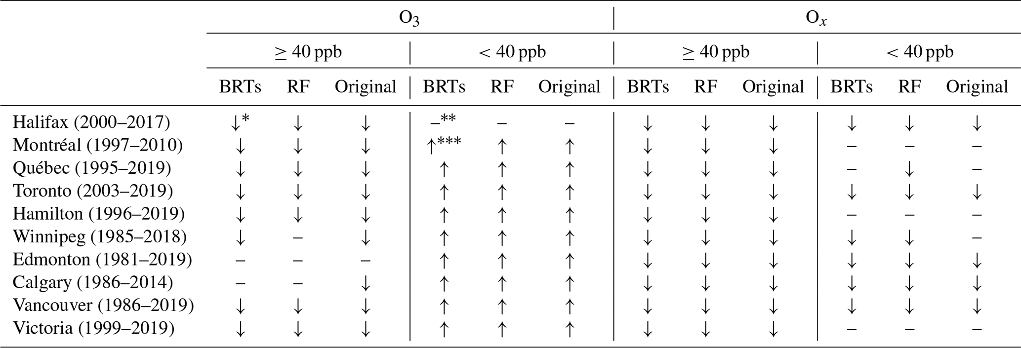
Table 3 Trends in deweathered and original annual average O₃ and O_x mixing ratios at levels below and above 40 ppb in 10 Canadian cities during the last decades (^* decreasing tends with P<0.05; ${}^{**}$ no trend or stable trend with P>0.10; ${}^{***}$ increasing trend with P<0.05).

4.2 Trend analysis of O₃ net sinks and sources

As reported in literature, a large fraction of ground-level O₃ at middle-to-high latitude zones comes from secondary reactions associated with natural sources (Barrie et al., 1988; Van Dam et al., 2013; Cooper et al., 2005; Seinfeld and Pandis, 2006; Mitchell et al., 2021). The natural signal usually has a spring maximum related to stratosphere–troposphere exchange as well as increasing photochemistry, among other potential factors (Chan and Vet, 2010; Monks et al., 2015; Strode et al., 2018; Xu et al., 2019). The contributions from stratosphere–troposphere exchange are approximately 40 ppb, while the sinks associated with natural and anthropogenic factors in the atmospheric boundary layer may decrease the ground-level O₃ to levels lower than 40 ppb (Barrie et al., 1988; Van Dam et al., 2013; Chan and Vet, 2010; Monks et al., 2015; Mitchell et al., 2021). On the other hand, enhanced tropospheric photochemical reactions under favorable meteorological conditions may increase the ground-level O₃ to levels higher than 40 ppb, causing severe O₃ pollution (Monks et al., 2015; Simon et al., 2015; Seinfeld and Pandis 2006; Xu et al., 2019). In fact, 40 ppb has been widely used as the threshold value for assessing O₃ impacts on ecosystem health (e.g., the AOT40 index) (Avnery et al., 2011). Thus, O₃ data with mixing ratios lower and higher than 40 ppb were analyzed separately below, with the former case representing net O₃ sinks occurring in the atmospheric boundary layer and the latter one representing net O₃ sources occurring therein (Table 3).

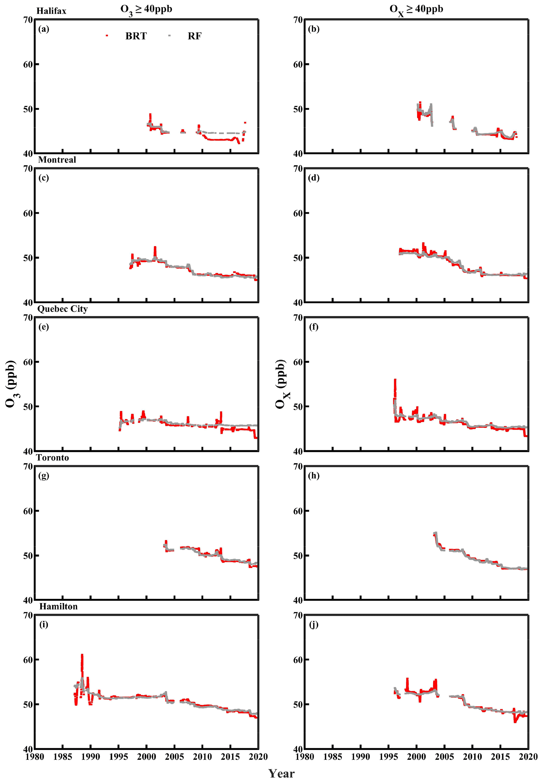
Figure 4 Deweathered hourly mixing ratios of O₃ (left column) and O_x (right column) at levels ≥40 ppb in five eastern Canadian cities.

In the cases with O₃ mixing ratios ≥40 ppb, the deweathered and original values, however, exhibited decreasing trends (P<0.05) in all of the five eastern cities and two western cities (Victoria and Vancouver) (Figs. 4 and S8 and Table 3). The overall decreases in O₃ with mixing ratios ≥40 ppb were 2 ppb in Halifax from 2000–2017, in Montréal and Québec from 1995–2019, and in Victoria from 1999–2019 (figure not provided); 4 ppb in Toronto from 2003–2019; 5–6 ppb in Hamilton from 1987–2019; and 12 ppb in Vancouver from 1986–2019 (but only 2 ppb from 2000–2019). Again, a few spikes and troughs occurred in the BRT-deweathered values possibly because of unpredictably increased and decreased emissions of O₃ precursors, respectively. In the cases with O_x mixing ratios ≥40 ppb, the decreasing trends were obtained in all of the 10 cities. These results further implied that the tropospheric photochemical formation of O₃ likely reduced in 7 of the 10 cities during the last 2 to 3 decades.

In the cases with O₃ mixing ratios ≥40 ppb in the remaining three western cities, the decreasing trends (P<0.05) were obtained in the BRT-deweathered and original values and no significant trend (P>0.05) in the RF-deweathered values in Winnipeg; the decreasing trend was obtained only in the original values in Calgary; and no significant trends in the deweathered and original values in Edmonton. These trend results implied that the responses of the fraction of O₃ to emission reductions of its precursors were too weak to be confirmed, especially in the presence of perturbation due to varying weather conditions.

In the cases with O₃ mixing ratios <40 ppb, the trends were almost the same as those from using the full dataset of O₃ mixing ratios. This consistency suggested that the increasing trends in O₃ mixing ratio in the nine Canadian cities were mainly due to the reduced O₃ sinks.

4.3 The perturbation from large-scale wildfires on PM_2.5 trend in western Canadian cities

Wildfire emissions become important contributors to air pollution in North America with global warning and increased extreme weather conditions such as heat waves and severe droughts (Andreae and Merlet, 2001; Littell et al., 2009; Marlon et al., 2013; Barbero et al., 2015; Abatzoglou and Williams, 2016; Randerson et al., 2017; Mardi et al., 2021). For example, Meng et al. (2019) estimated that wildfires accounted for 17.1 % of the total population-weighted exposure to PM_2.5 for Canadians during 2013–2015 and 2017–2018. The large contribution was not surprising, because large wildfires can rapidly increase hourly PM_2.5 mass concentration from a few µg m⁻³ to >400 µg m⁻³ (Landis et al., 2018 and Fig. S1). The estimated annual economic cost attributable to PM_2.5 pollution reached CAD 410 million to USD 1.8 billion for acute health impacts and CAD 4.3 billion to CAD 19 billion for chronic health impacts in western Canada (Landis et al., 2018; Matz et al., 2020). In the USA, wildfire emissions were reported to account for up to 25 % of annual primary PM_2.5 emissions (Barbero et al., 2015).

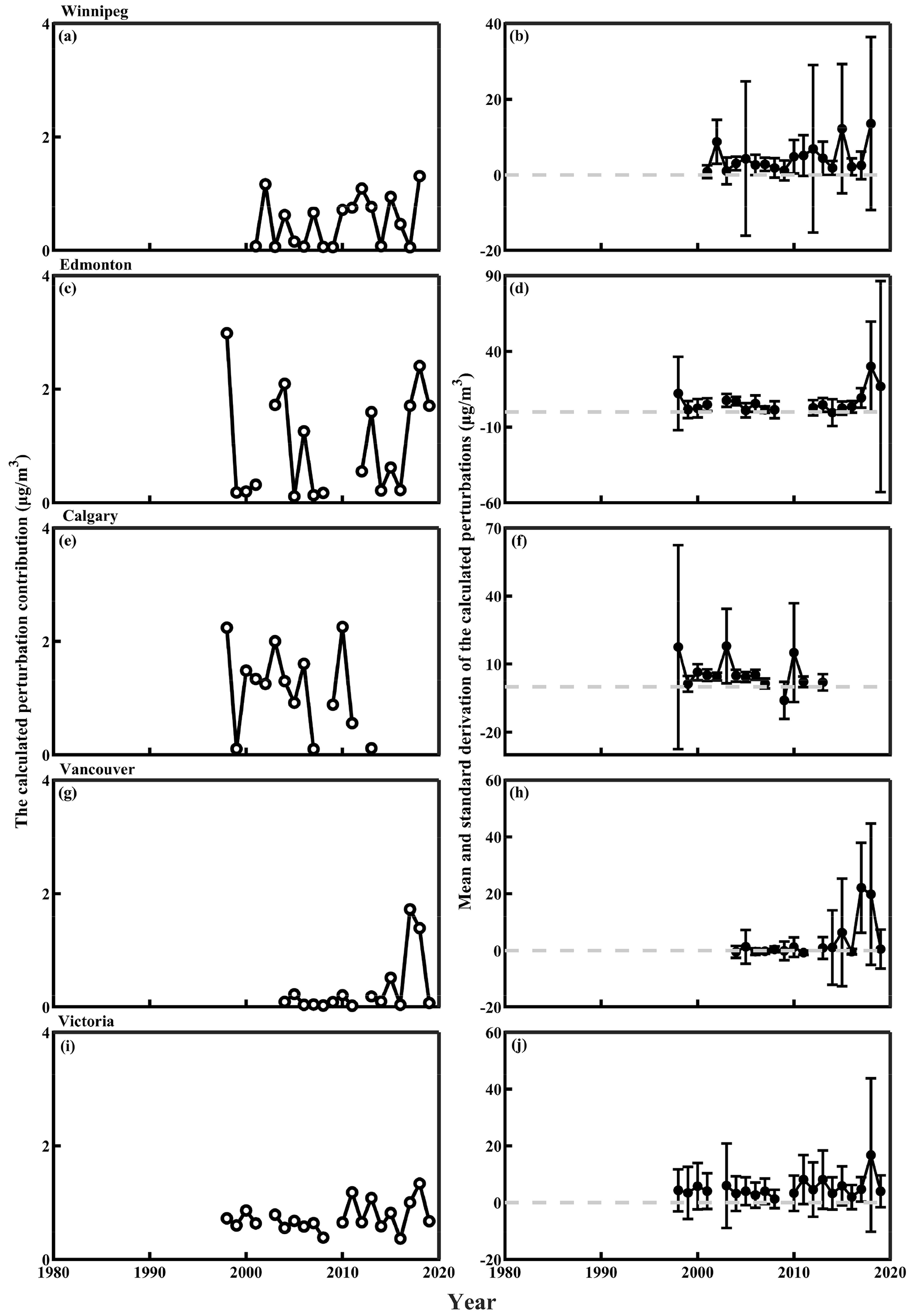
Figure 5 The calculated perturbation contribution to the corresponding original annual average PM_2.5 concentration (left column) and the mean and standard derivation of the calculated perturbation (right column) in five western Canadian cities.

Due to the wide occurrence of small-scale wildfires, most of the emitted air pollutants from these sources and subsequent long-range transport can be considered natural background pollution. The key issue is to quantify the abnormally increased contributions from large-scale wildfires to annual average PM_2.5 in each year and their perturbations on long-term trends in PM_2.5. Using the method described in Sect. 2, the perturbation contributions in Winnipeg were estimated to be around $\mathrm{0.5}.\pm \mathrm{0.4}$ µg m⁻³ in 2001–2018, with larger values of 1.1–1.3 µg m⁻³ associated with large-scale wildfires in 2002, 2012 and 2018 (Fig. 5a). The larger perturbation contributions in 2012 and 2018 indeed led to an increasing trend in PM_2.5 from 2001–2018 in this city (Table 2). The perturbation contributions were, however, smaller than 0.2 µg m⁻³ in 2001, 2003, 2005, 2006, 2008, 2009, 2014 and 2017, and such small values may be related to varying weather conditions rather than large-scale wildfires.

In Edmonton, the perturbation contributions were around 1.0±0.9 µg m⁻³ in 1998–2019 (Fig. 5b). However, the largest contribution was 3.0 µg m⁻³ in 1998, followed by 2.4 µg m⁻³ in 2018 and 2.1 µg m⁻³ in 2004, respectively, because of large-scale wildfires. The perturbation contributions from large-scale wildfires were large enough to cancel out the mitigation effect of air pollutants on annual averages of PM_2.5 in Edmonton. In Calgary, the perturbation contributions were around $\mathrm{1.2}.\pm \mathrm{0.7}$ µg m⁻³ in 1998–2013, depending on if large-scale wildfires occurred in any particular year. For example, the perturbation contributions were smaller than 0.2 µg m⁻³ in 1999, 2007 and 2013, while the contributions reached 2.2–2.3 µg m⁻³ in 1998 and 2010.

In Victoria, the perturbation contributions were around 0.7±0.2 µg m⁻³ in 1998–2019. The perturbation contribution in each year was, however, larger than 0.4 µg m⁻³, suggesting that the wildfires were always important contributors. In Vancouver, the perturbation contributions largely decreased to $\mathrm{0.3}.\pm \mathrm{0.5}$ µg m⁻³ in 2004–2019. However, the maximum value still reached 1.7 µg m⁻³ in 2017, followed by 1.4 µg m⁻³ in 2018 and 0.5 µg m⁻³ in 2015. The large perturbation likely overwhelmed or canceled out the effects of emission reductions on annual average PM_2.5.

5 Conclusions

Through analysis of deweathered and original annual average concentrations of selected criteria air pollutants measured in 10 major cities in Canada during the last 2 to 3 decades, we have generated the following decadal trends for these pollutants: (1) decreasing trends in NO₂, CO and SO₂ mainly due to reduced primary emissions across Canada, except no significant trend in CO in Montréal; (2) increasing trends in O₃ mainly due to the reduced titration effect across Canada, except no significant trend in O₃ in Halifax; and (3) roughly opposite trends in PM_2.5 between eastern and western Canada, resulting from the combined effects of emission reductions and the occurrence of large-scale wildfires.

The overall percentage decrease in NO₂ during the last 2 to 3 decades among the 10 cities ranged from 37 % to 62 %, and the annual decreasing rates varied from 0.31 to 0.74 ppb yr⁻¹. The overall percentage decrease in CO varied from 57 % to 92 % and the annual decreasing rate ranged from 0.010 to 0.076 ppm yr⁻¹ between nine cities. The corresponding numbers for SO₂ are from 23 % to 93 % and from 0.04 to 0.63 ppb yr⁻¹ among the 10 cities. By only considering O₃ mixing ratio ≥40 ppb, annual average O₃ decreased by 2–4 ppb in most cities during the past 2 to 3 decades but not in Calgary and Edmonton, and no consistent decreasing trend was identified in Winnipeg, implying that the mitigation effects of air pollutants on O₃ were too weak to be confirmed.

The mitigation effects on PM_2.5 were detected on the basis of the identified decreasing trends in three of the five eastern cities regardless of using original or deweathered annual average data, but this is not the case in the other two eastern cities. In the five western cities, the perturbation due to large-scale wildfires greatly affected original annual average PM_2.5 and was large enough to cancel out the mitigation effects in some years, leading to no decreasing trends and in some cases even increasing trends.

Excluding Calgary, the annual average AQHI showed a significant decrease by 8 %–29 % during the last 2 decades to levels between 1.8 and 3.0 in 2017–2019. However, large-scale wildfire events still occasionally elevated AQHI to a level of above 10 (very high risk) (<0.3 % frequency) in western Canadian cities after 2010. Thus, large-scale wildfires have become a key factor in causing severe air pollution in Canadian cities, as was seen in the most recent very large scale wildfires occurring in Canada from the later spring to the earlier summer in 2023 that resulted in severe air pollution across Canada and New York through long-range transport. Urgent work should be conducted for assessing the impacts of large-scale wildfires on human health and climate change, besides investigating their occurrence and control mechanisms and transport pathways. In-depth studies are also needed to explore the causes of the non-decreasing trends in O₃ with mixing ratios ≥40 ppb in some western Canadian cities, results from which are critical for making future control policies.