the Creative Commons Attribution 4.0 License.
the Creative Commons Attribution 4.0 License.
 | 03 Jul 2024
The influence of extratropical cross-tropopause mixing on the correlation between ozone and sulfate aerosol in the lowermost stratosphere
Johannes Schneider
Katharina Kaiser
Horst Fischer
Peter Hoor
Daniel Kunkel
Hans-Christoph Lachnitt
Andreas Marsing
Lenard Röder
Hans Schlager
Laura Tomsche
Christiane Voigt
Andreas Zahn
Stephan Borrmann
The chemical composition of the upper troposphere/lower stratosphere region (UTLS) is influenced by horizontal transport of air masses, vertical transport within convective systems and warm conveyor belts, rapid turbulent mixing, as well as photochemical production or loss of species. This results in the formation of the extratropical transition layer (ExTL), which is defined by the vertical structure of CO and has been studied until now mostly by means of trace gas correlations. Here, we extend the analysis to include aerosol particles and derive the sulfate–ozone correlation in central Europe from aircraft in situ measurements during the CAFE-EU (Chemistry of the Atmosphere Field Experiment over Europe)/BLUESKY mission. The mission probed the UTLS during the COVID-19 period with significantly reduced anthropogenic emissions. We operated a compact time-of-flight aerosol mass spectrometer (C-ToF-AMS) to measure the chemical composition of non-refractory aerosol particles in the size range from about 40 to 800 nm. In our study, we find a correlation between the sulfate mass concentration and O3 in the lower stratosphere. The correlation exhibits some variability exceeding the mean sulfate–ozone correlation over the measurement period. Especially during one flight, we observed enhanced mixing ratios of sulfate aerosol in the lowermost stratosphere, where the analysis of trace gases shows tropospheric influence. However, back trajectories indicate that no recent mixing with tropospheric air occurred within the last 10 d. Therefore, we analyzed volcanic eruption databases and satellite SO2 retrievals from the TROPOspheric Monitoring Instrument (TROPOMI) for possible volcanic plumes and eruptions to explain the high amounts of sulfur compounds in the UTLS. From these analyses and the combination of precursor and particle measurements, we conclude that gas-to-particle conversion of volcanic SO2 leads to the observed enhanced sulfate aerosol mixing ratios.
- Article
(14994 KB) - Full-text XML
- BibTeX
- EndNote


The chemical composition of upper-tropospheric aerosol particles is highly variable because primary aerosols from natural and anthropogenic ground sources reach this altitude (Martinsson et al., 2019), and secondary aerosols are formed here from gas-to-particle conversion. However, the stratospheric aerosol composition is less complex as the main component is particulate sulfate (SO) with concentrations between 0.1 and 40 µg m−3 accompanied by minor tropospheric compounds (Deshler, 2008; Murphy et al., 2013; Brimblecombe, 2014; Kremser et al., 2016).
The stratospheric aerosol layer, also known as the Junge layer (Junge and Manson, 1961), is part of the lowermost stratosphere (LMS) and is located roughly between 15 and 25 km (Hofmann and Rosen, 1981). The chemical composition of the aerosol layer underlies seasonal variations induced by the Brewer–Dobson circulation (Martinsson, 2005; Friberg et al., 2014) and volcanic activity, which may increase the aerosol optical depth (AOD) by up to 40 % (Friberg et al., 2018). Sulfate aerosol is formed due to oxidation of carbonyl sulfide (OCS) and sulfur dioxide (SO2) (Crutzen, 1976; Brühl et al., 2012; Solomon et al., 2011; Kremser et al., 2016) and has an average radius under undisturbed conditions of 170 nm (e.g., Tilmes and Mills, 2014). Both precursor gases have their main sources in the troposphere. OCS is the main sulfur-containing trace gas in the atmosphere, with direct emissions by the oceans or biomass burning as well as photochemical production by oceanic emissions like dimethyl sulfide (DMS) or carbon disulfide (CS2) (Andreae, 1990; Brühl et al., 2012; Kremser et al., 2016). SO2 is primarily emitted by industrial processes like the fossil fuel burning. While degassing volcanoes contribute to the tropospheric SO2 budget (Voigt et al., 2014), explosive eruptions can directly inject SO2 into the lower stratosphere (Kremser et al., 2016). Other direct sulfate aerosol sources are aircraft which emit soot and volatile sulfate-containing particles at cruise altitudes into the upper troposphere/lower stratosphere (UTLS) (Voigt et al., 2010; Williamson et al., 2021; Tomsche et al., 2022).
Transport processes of aerosol particles into the UTLS have been the subject of several studies, for example with a focus on tropical processes or the Asian tropopause aerosol layer (ATAL) (e.g., Appel et al., 2022; Fadnavis et al., 2013; Froyd et al., 2009; Höpfner et al., 2019). Tracer correlations of aerosol particles with ozone (O3) and nitrous oxide (N2O) based on high-altitude in situ measurements have also been used in the context of polar vortex dynamics after a major volcanic eruption (Borrmann et al., 1993, 1995). In those studies, the temporal evolution of the correlation between the mixing ratios of sulfate aerosol, surface area for aerosol particles with a size between roughly 10 nm and more than 1 µm as well as O3 inside and outside of the polar vortex was analyzed over the course of 22 months after the Mt. Pinatubo eruption in 1991. The observations revealed a slow development of a linear correlation between the O3 versus aerosol number and surface mixing ratios in the midlatitude UTLS, which degraded again later on. This demonstrated the suitability of aerosol properties as dynamical tracers once the microphysical processes like new particle formation, coagulation and condensational growth following a volcanic eruption into the stratosphere ceased. Furthermore, a temporally stable equilibrium of particle size or surface area has been established.
In the extratropics, the chemical composition of the tropopause region is influenced not only by the Brewer–Dobson circulation, but also by convection, mixing along the subtropical and polar frontal jet streams, breaking of gravity and Rossby waves as well as vertical wind shear (e.g., Gettelman et al., 2011; Kaluza et al., 2021). This forms a transition layer above the tropopause called the extratropical transition layer (ExTL), where tropospheric as well as stratospheric influence is observed (Hoor et al., 2004; Hegglin et al., 2009; Gettelman et al., 2011; Konopka and Pan, 2012; Barré et al., 2013). The effect of these small-scale mixing processes on the chemical composition of aerosol particles in the ExTL has not been well known until now (Kunkel et al., 2019). The lifetime of atmospheric aerosol particles with diameters lower than 1 µm can reach 1 month or more (Jaenicke, 1980). This is sufficient for the particles to be transported up into the tropopause region over long distances and, subsequently, by mixing processes into the stratosphere. Furthermore, the lifetime of more than 1 month corresponds to the timescale that gas-to-particle conversion needs to form sulfate aerosol particles from SO2 as a precursor gas in the UTLS (Jurkat et al., 2010; Gorkavyi et al., 2021; Rollins et al., 2017).
In our study, we use tracer–tracer correlations as a tool for mixing diagnostics to identify stratospheric air masses and the underlying mixing processes. The basic principle of this method is to use a tropospheric tracer with sources in the troposphere and a rather constant stratospheric background, e.g., carbon monoxide (CO) and water vapor (H2O), and a tracer with only a stratospheric increase or decrease and a fairly constant mixing ratio in the troposphere, e.g., O3 or N2O. In a scatterplot with the tropospheric tracer on the abscissa and the stratospheric tracer on the ordinate, one would expect two separated reservoirs that are not connected if no mixing processes occur. If mixing takes place, both reservoirs are connected by mixing lines, where the mixing ratios are between the two regimes, depending on the state of mixing (Fischer et al., 2000; Hoor et al., 2002).
With this study we want to introduce particulate sulfate as a stratospheric tracer in the correlation with O3 and find processes that are responsible for the variability of the correlation between sulfate aerosol and O3 mixing ratios. Therefore, we use in situ aircraft measurements from the CAFE-EU (Chemistry of the Atmosphere Field Experiment over Europe)/BLUESKY mission, conducted in spring 2020 from Oberpfaffenhofen, Germany.
2.1 Data overview
The CAFE-EU/BLUESKY measurement campaign was conducted with the research aircraft HALO (High Altitude and Long Range Research Aircraft) and DLR-Falcon, both operated by the German Aerospace Center (DLR). The measurement flights were performed over central Europe and the North Atlantic between 16 May and 9 June 2020, partly co-located with both aircraft (see Fig. 1). The measurements were conducted during the first COVID-19 lockdown in Germany and Europe, such that the main goal of the campaign was to investigate the atmospheric changes during reduced industrial activity and lower emissions compared to other times (Voigt et al., 2022). This point leads to flight planning during the campaign with a focus on urban areas and low-altitude profiles and less on studying processes in the UTLS region. Therefore, it was not possible to conduct measurements over the complete vertical extent of the ExTL during May 2020. Nevertheless, we were able to obtain measurement data up to 14 km altitude representing the chemical composition of the UTLS. During the campaign period, air traffic was significantly reduced over Europe by up to 80 % (Schumann et al., 2021a, b). Krüger et al. (2022) found substantial reduction in aerosol particles in the lower troposphere in this period, and Reifenberg et al. (2022) could explain the observed reduction in some tracer concentrations with the reduced emissions of pollutants. Tomsche et al. (2022) investigated the SO2 concentrations in the UTLS region above Europe, which was influenced by changes in sulfur sources such as aviation as well as sinks. Here we focus on the transport processes in the extratropical transition layer, which has been probed with a set of instrumentation on board HALO and DLR-Falcon.
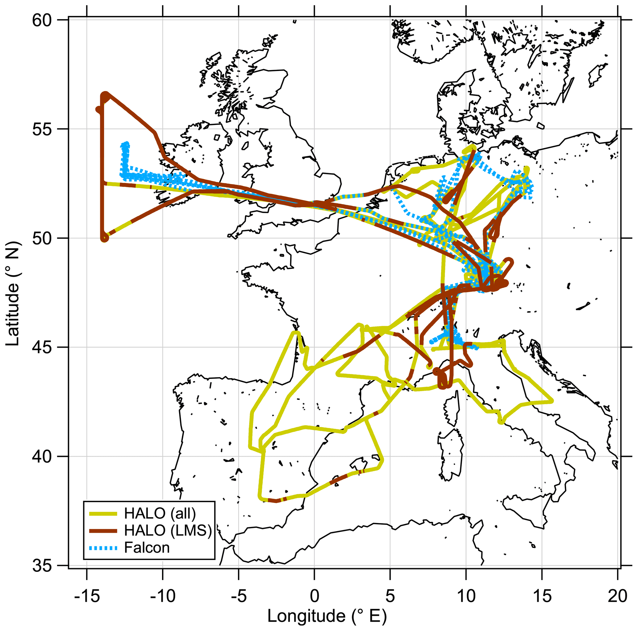
Figure 1Overview map of all measurement flights performed during the CAFE-EU/BLUESKY measurement campaign between 16 May and 9 June 2020. The HALO flight path as solid line is divided into the complete dataset (yellow) and stratospheric (brown) segments, while the DLR-Falcon flight path is shown as a dashed blue line.
2.2 Instrumentation
For our study, we use the chemical composition of aerosol particles measured on board HALO and trace gas measurements on board HALO and DLR-Falcon. The chemical composition of non-refractory aerosol particles was measured on HALO with a compact time-of-flight aerosol mass spectrometer (C-ToF-AMS) for particles in the size range between 40 and 800 nm (Drewnick et al., 2005; Schulz et al., 2018) and with this within the same size range as previous studies (e.g., Borrmann et al., 1995). We obtain quantitative information on the mass concentration of sulfate, nitrate, ammonium, organic matter and chloride normalized to STP (standard temperature and pressure) conditions. The measurement interval of the C-ToF-AMS during the campaign was 30 s, resulting in a spatial resolution of about 6 km in the UTLS region. The accuracy of the AMS is about 30 % (Bahreini et al., 2009; Canagaratna et al., 2007; Middlebrook et al., 2012). In the following, we use the mixing ratio instead of the mass concentration for comparison with the trace gas measurements. Integrated into the C-ToF-AMS, we use an optical particle counter (OPC) manufactured by GRIMM (OPC 1.129) to measure the aerosol size distribution in 31 size channels from 250 nm to larger than 32 µm.
In addition to the aerosol chemical composition and size data, we use trace gas measurements, like SO2, CO, H2O, O3 and nitric acid (HNO3), on board HALO and DLR-Falcon.
CO measurements on HALO were performed with the quantum cascade laser absorption spectrometer TRISTAR (Tadic et al., 2017; Röder et al., 2023) with a total measurement uncertainty of 3 % at 10 s time resolution. O3 on HALO was measured by FAIRO, which measured on the basis of a UV photometer and chemiluminescence (Zahn et al., 2012). On board DLR-Falcon, CO and O3 were measured with a cavity ring-down spectrometer (PICARRO G2401) and a dual-cell UV photometer (TE 49C), respectively. Both instruments were calibrated before and after the flights with standards that can be traced back to the GAW Hohenpeissenberg station. The precision and accuracy of the CO and O3 measurements are 3 ppbv/5 ppbv and 3 %/5 %, respectively. An additional in situ dataset is provided by the atmospheric chemical ionization mass spectrometer (AIMS) deployed on DLR-Falcon and includes information on gaseous SO2, HNO3 and SF5 (pentafluorosulfanyl). For the detection of upper-tropospheric and lower-stratospheric SO2 and HNO3 mixing ratios, the AIMS uses SF reagent ions (Voigt et al., 2014; Jurkat et al., 2016; Marsing et al., 2019; Tomsche et al., 2022). The 1-sigma detection limit is 0.0006 to 0.0017 ppbv and 0.005 to 0.009 ppbv for SO2 and HNO3, respectively. The total uncertainty for SO2 is 22.7 % (Tomsche et al., 2022) and 16 % for HNO3 (Ziereis et al., 2022).
2.3 Meteorology and trajectories
In addition to the in situ measurement data, we use model data interpolated onto the flight path of both aircraft. For meteorological information, we use the ERA5 reanalysis dataset with a temporal resolution of 6 h and a grid spacing of 1° in the horizontal and a vertical spacing of approximately 500 m in the UTLS (Hersbach et al., 2020). Based on the native variables, we additionally calculated potential vorticity (PV) and equivalent latitude. The equivalent latitude is a framework to account for reversible transport under adiabatic conditions and thus get information on potential diabatic transport or mixing. For the calculation, for different isentropes a PV contour line with the same potential vorticity and potential temperature is transformed into a pole-centered circle. The equivalent latitude is the enclosing latitude of this circle (e.g., Lary et al., 1995; Hegglin et al., 2006; Krause et al., 2018). These calculations are done over isentropic surfaces from 240 up to 2000 K from the ERA5 reanalysis data interpolated onto potential temperature.
For our analysis of the air mass origin and possible transport pathways, we use trajectories calculated with the Lagrangian analysis tool (LAGRANTO; Sprenger and Wernli, 2015). Therefore, we initialize a set of 231 trajectories every 30 s along the flight path. The starting points of each trajectory set are placed in a three-dimensional cross around the initial point of the flight path to gain a better statistic and to minimize interpolation errors between the measurements and the model grid. More specifically, we take the location of the aircraft and add five additional points every 0.01° in all four horizontal directions (north, east, south and west), resulting in 21 points arranged in a cross shape (including the aircraft position and location). This cross pattern of 21 points is repeated at 10 additional vertical levels in 1 hPa steps, 5 levels above the flight altitude and 5 levels below the flight altitude. Thus, we get a total of 231 trajectory starting locations at each release time, providing information for 10 d back in time with quantities such as potential temperature and potential vorticity.
3.1 Part 1: correlation of particulate sulfate and ozone
O3 is a suitable tracer for identifying stratospheric air masses due to the photochemical production of O3 in the stratosphere and its low abundance in the troposphere and its local chemical lifetime of years in the lower stratosphere. There are several ways of identifying the tropopause and thus the lower boundary of the stratosphere from measured O3 mixing ratios. For example, fixed threshold values of typically 70 or 100 ppbv have been used (e.g., Bethan et al., 1996; Staehelin, 2003). This method has the disadvantage of neglecting the seasonal cycle of O3, and thus the threshold value can be too low or too high when periods exceeding 1 month are analyzed. Another way of determining the O3-based tropopause is to take the seasonal cycle into account by using a daily threshold for the O3 tropopause. This method is described in Zahn et al. (2004) and Thouret et al. (2006) on the basis of long-term observations. In our study we use the method of Zahn et al. (2004) to calculate daily O3 thresholds for the tropopause. Figure 2 shows the seasonal cycle of the O3 mixing ratio at the chemical tropopause and the 2 PVU (potential vorticity units, 10−6 m2 s−1 K kg−1) dynamical tropopause, both calculated following Zahn et al. (2004). For the period of our study (16 May to 9 June), we only see small differences in the results between the chemical and dynamical tropopause since both thresholds are close together around 120 ppbv O3 during the time of our measurements. We extracted all stratospheric data (i.e., all data points with O3 mixing ratios larger than the daily threshold) and calculated the frequency distribution of the potential vorticity from the ERA5 dataset (Fig. 2) to verify that the chemical tropopause inferred from the measured O3 mixing ratios and the calculated thresholds correspond to the dynamical tropopause. This shows that the vast majority of the stratospheric data points have PV values larger than 2 PVU. In Fig. 2, we observe two modes in the PV distribution of the stratospheric data which can be explained by the different stratospheric ages of the sampled air masses (Bönisch et al., 2009). The first mode results from air freshly mixed into the stratosphere with PV values close to the dynamical tropopause. The second mode with values larger than 8 PVU describes air originating from the high stratosphere with no tropospheric influence. In total, less than 4 % of the stratospheric data points have PV values below the 2 PVU threshold. Thus, we use the definition of the chemical tropopause based on O3 mixing ratios following Zahn et al. (2004) in this study.
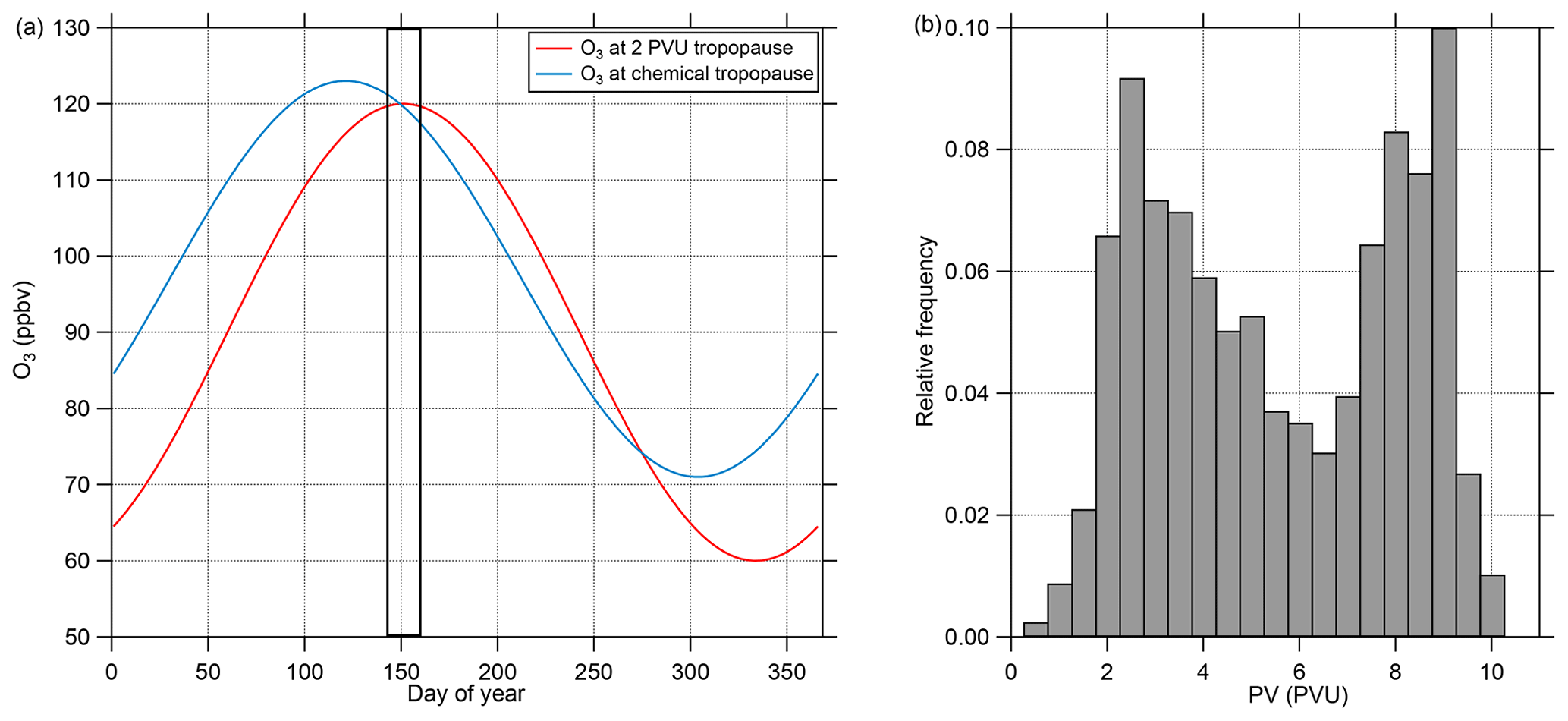
Figure 2(a) Calculated seasonal cycle of O3 mixing ratios at the 2 PVU dynamical tropopause and the chemical tropopause, both calculated following Zahn et al. (2004). The measurement period is marked with the solid frame. (b) Relative frequency of PV values interpolated to the AMS data points from CAFE-EU/BLUESKY identified as stratospheric using the calculated O3 mixing ratios at the chemical tropopause. Less than 4 % of the data points show PV values lower than 2 PVU, indicating a negligible amount of tropospheric air. The complete stratospheric dataset holds 2049 data points, which represent 100 % of this subset.
Besides O3, there are other trace gases used as indicators of stratospheric air masses, e.g., H2O or N2O. Moreover, within limits, aerosol particle properties can be applied as well (Borrmann et al., 1993, 1995). A good example is the mass concentration of particulate sulfate, which increases in the stratosphere due to the formation from precursors, which takes 30 to 60 d and reaches its maximum in the Junge layer, where particulate sulfate is present in the form of binary solution droplets with inclusions of sulfuric acid (Junge and Manson, 1961; Brühl et al., 2012; Kremser et al., 2016). Thus, we expect a positive correlation between particulate sulfate and O3 in the stratosphere. The observations made on HALO during the CAFE-EU/BLUESKY campaign confirm this (Fig. 3). Here, two distinct regimes appear in the correlation plot of particulate sulfate and O3. In the tropospheric regime, the sulfate mass concentration shows high variability at O3 levels below 100 ppbv, depending on the source regions within the boundary layer, e.g., industrial areas. In the stratosphere, we observe a linear correlation between the two species with a slope of 900 to 2300 ppbv ppbv−1, but with variations between the individual measurement flights, i.e., on short timescales of a few days. Note that the accuracy of the C-ToF-AMS of about 30 % (Bahreini et al., 2009) does not affect the observed different slope regimes in the correlation of sulfate aerosol and ozone, because the quantities determining the accuracy (ionization efficiency, collection efficiency and inlet transmission efficiency) do not change over the short period of a 2-week measurement campaign.
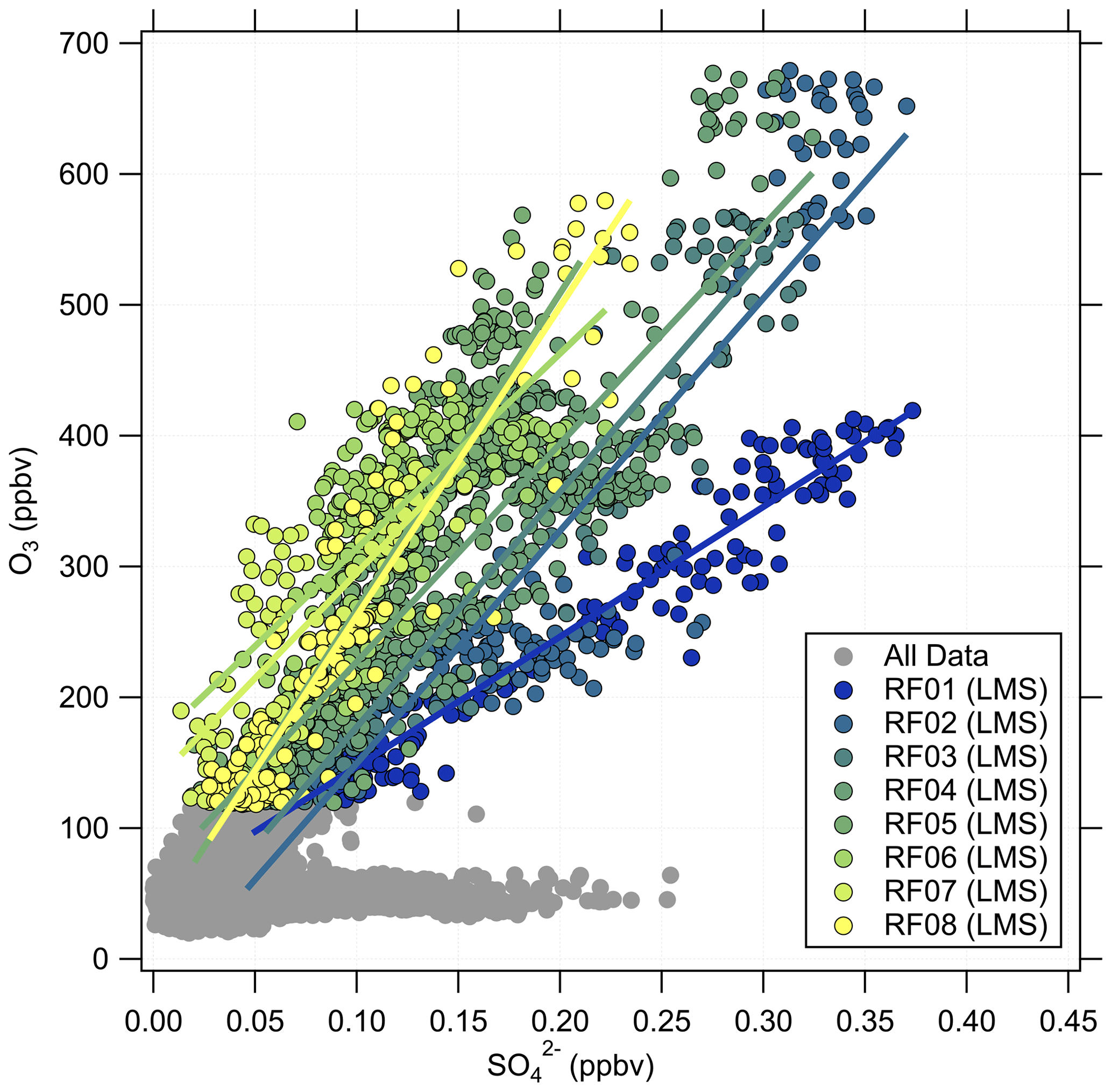
Figure 3Correlation between the particulate sulfate mixing ratio and the O3 mixing ratio for the full CAFE-EU/BLUESKY dataset. The color-coded data points indicate the stratospheric data derived from the chemical tropopause O3 mixing ratios. The grey data show the complete dataset, including the tropospheric data. The solid color-coded lines represent the linear regressions for the individual flights.
This analysis shows that the correlation between particulate sulfate and O3 can be used as a tool for analyzing air masses in terms of their stratospheric character. The variations in the slope and compactness of the correlation appear on short timescales of a few days. The aim of this study is to understand these variations and link them to possible atmospheric processes. There are a number of different pathways by which sulfur species can be transported from the troposphere into the stratosphere and thus be a possible reason for the observed variability (e.g., Kremser et al., 2016). Feinberg et al. (2019) show the modeled atmospheric sulfur budget under volcanically quiescent conditions and the pathways that lead to the formation of particulate sulfate in the stratosphere. Among these pathways, the most efficient one is the mixing of precursor gases such as OCS and SO2 into the stratosphere, where OCS is oxidized to SO2 and SO2 is further converted to sulfuric acid, forming sulfate aerosol. It is important to emphasize that this budget is valid for volcanically quiescent conditions, because in the presence of volcanic eruptions an additional large source of SO2 adds up to the other pathways. In this case, SO2 is transported in the eruption column up into the free troposphere or even the UTLS region, depending on the strength of the eruption. Then SO2 is converted to sulfuric acid and particulate sulfate, also in the upper troposphere or even in the stratosphere (Kremser et al., 2016).
The low sulfate mixing ratios at the chemical tropopause (Fig. 3) show that direct mixing of high sulfate aerosol concentrations from the troposphere to the stratosphere was not observed during the campaign, so some other processes need to be taken into account. This observation of low particulate sulfate aerosol amounts at the chemical tropopause is very robust over the whole campaign period, and there it might be controlled by atmospheric processes that need more investigation.
Previous studies with a focus on the Raikoke eruption in 2019 determined no significant contribution from this volcanic eruption (Tomsche et al., 2022; Reifenberg et al., 2022). The following section will show the possible influence of cross-tropopause mixing, especially of the precursor gas SO2 and the potential influence of a more recent volcanic eruption.
3.2 Part 2: case study on aerosol chemical composition related to mixing processes
Volcanic influence is one of the possibilities that can explain the observed variability in the correlation. One major eruption occurred in 2019 with the Raikoke volcano. However, Tomsche et al. (2022) and Reifenberg et al. (2022) showed that this eruption did not have a significant impact on the measurements during CAFE-EU/BLUESKY. In the following, we focus on a case study to explain the variability of the particulate sulfate correlation with O3, especially for research flight RF01, as the slope in the O3–SO correlation for this flight clearly differs from the other flights (see Fig. 3).
The anticorrelation between CO and O3 can be used to identify mixing processes between the troposphere and stratosphere (Fischer et al., 2000; Hoor et al., 2002). The presence of mixing lines connecting the sampled tropospheric and stratospheric air masses indicates recent mixing processes. In Fig. 4, most of the stratospheric data of the whole campaign dataset lie in a region of anticorrelated CO and O3. Thus, it can be concluded that the measured air masses in the stratosphere are influenced by tropospheric air that was mixed across the tropopause. As expected, the correlation in Fig. 4b shows much higher particulate sulfate mixing ratios at higher O3 levels in the stratosphere and lower mixing ratios close to the tropopause. However, we can identify an anomaly of high particulate sulfate mixing ratios (yellow points) at about 400 ppbv O3 and 40 ppbv CO (see also Figs. C1 and C4). Here, the measured mixing ratios of sulfate aerosol are in the range we would expect higher up in the stratosphere.
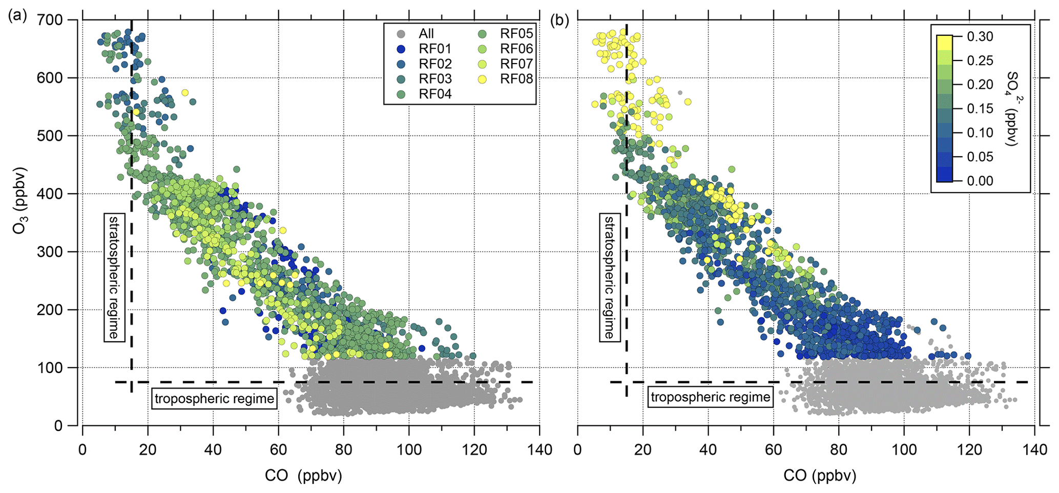
Figure 4(a) CO–O3 correlation for all data points in grey and the stratospheric data color-coded with the flight numbers. (b) The same correlation, but the stratospheric data are color-coded with the sulfate aerosol mixing ratio. In addition, the dashed lines indicate the mean tropospheric and stratospheric regimes without mixing processes.
In the following, we will analyze whether this anomaly is caused by a cross-tropopause mixing event and whether such events can explain the observed variability in the SO4–O3 correlation. For this analysis, we binned our dataset along equivalent latitude, which can be used as a dynamical tracer (Butchart and Remsberg, 1986; Hegglin, 2005), and potential temperature to see where the anomaly is located (see Fig. 5). The observed sulfate anomaly occurs in Fig. 5b between 40 and 45° N at potential temperatures between 345 and 350 K. It is not connected to the observed stratospheric aerosol layer that starts at higher altitudes, above the 370 K isentrope (see Fig. 5). The potential vorticity indicates that this region is in the vicinity of the jet stream, and with this mixing processes might have occurred or even be present. The O3 distribution does not show such an anomalous observation as found in the particulate sulfate (Fig. 5a), but we can observe the expected increase from the troposphere to the stratosphere. This location of the anomaly is in good agreement with the previous observation that the anomaly is located on a mixing line in the CO–O3 correlation in a transition regime between the troposphere and the stratosphere.
We further investigate the meteorology over the campaign period to determine whether the anomaly might be influenced by mixing processes. In particular, we use the vertical wind shear S2 and the static stability N2 (see also Appendix B) to identify regions with higher potential for mixing processes. Kaluza et al. (2021) and Kunkel et al. (2019) showed in their study that, in regions with high vertical wind shear ( s−2), conditions are favorable for rapid mixing. Figure 6 shows the analysis of the stability parameters mentioned above along with the resulting gradient Richardson number. The vertical wind shear shows high values in the region of the sulfate anomaly (see Fig. 6b), exceeding the mentioned threshold for enhanced mixing. This also results in a reduction in the gradient Richardson number in the same bin to values close to the critical threshold of 0.25 (see Fig. 6c), which indicates favorable conditions for turbulence. The static stability shows the expected transition from tropospheric to stratospheric values (see Fig. 6a). However, regarding the stability analysis, we probed several regions which show favorable conditions for instability and cross-tropopause mixing. Nevertheless, here we focus on the region with the strongest signal, where the observed sulfate anomaly was measured.
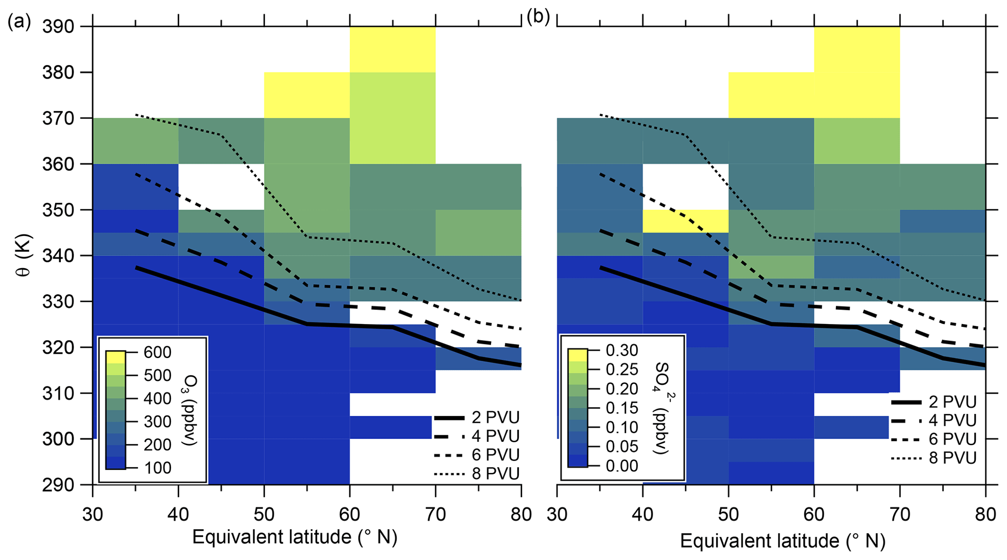
Figure 5Median of the O3 mixing ratio (a) and sulfate aerosol mixing ratio (b) in the θ-equivalent latitude space. Below 350 K, we use 5 K vertical resolution and 10∘-equivalent latitude bins. Above 350 K, we enlarge the vertical bins to 10 K to obtain a higher statistical evaluation basis (see Fig. A1). In general, only bins with more than 10 data points are evaluated. We added the 2 to 8 PVU lines to show the location of the dynamical tropopause and the extent of the ExTL into the stratosphere. We only show the region of interest for our study between 30 and 80° N.
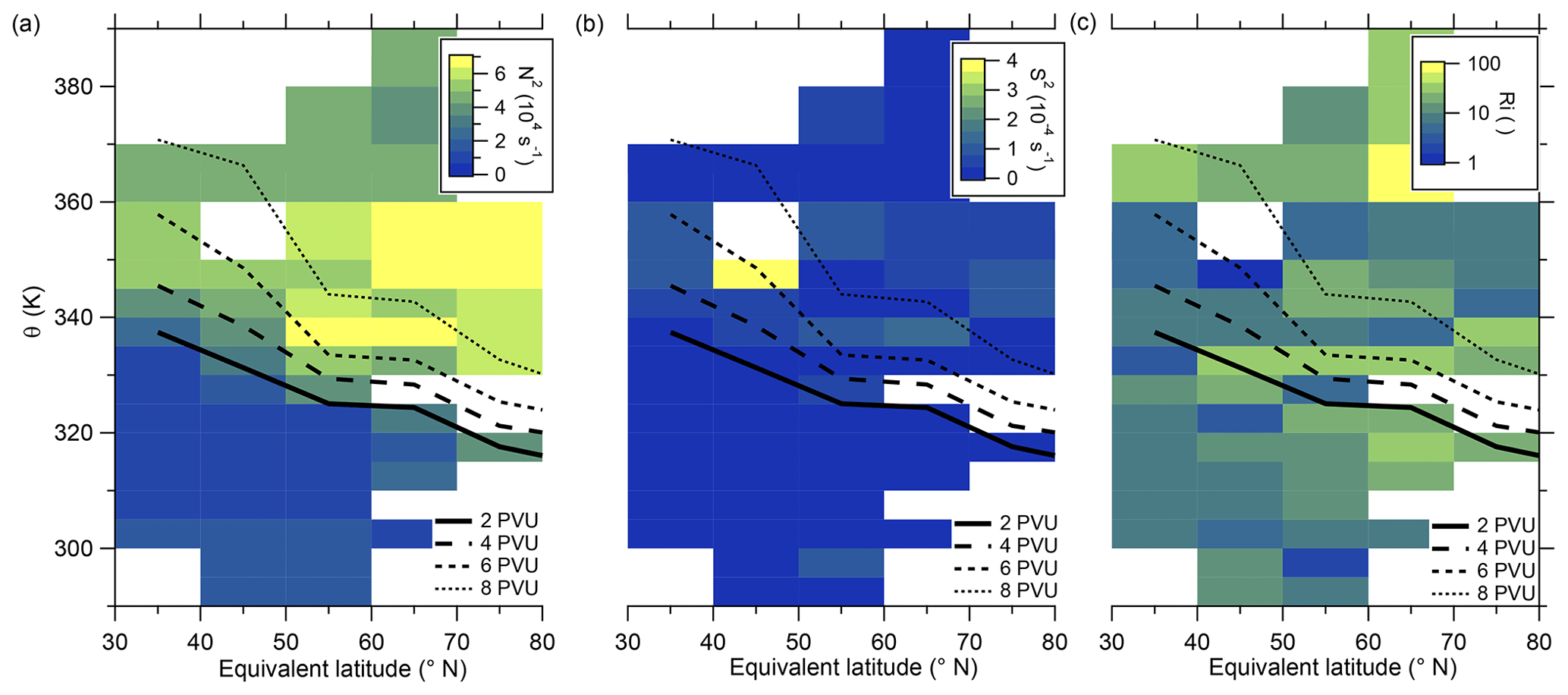
Figure 6Median of static stability N2 (a), vertical wind shear S2 (b) and gradient Richardson number (c) in the θ-equivalent latitude space. Below 350 K, we use 5 K vertical resolution and 10°-equivalent latitude bins. Above 350 K, we enlarge the vertical bins to 10 K to obtain a higher statistical evaluation basis (see Fig. A1). In general, only bins with more than 10 data points are evaluated. We added the 2 to 8 PVU lines to show the location of the dynamical tropopause and the extent of the ExTL into the stratosphere. We only show the region of interest for our study between 30 and 80° N.
These findings suggest that mixing occurred in this measurement region and is one influence on the variation of the SO4–O3 correlation. To prove this, we investigated the data in the region of the sulfate anomaly in more detail. Therefore, we extracted the data points that contribute to the anomaly. In total, there are 45 measurement points from the C-ToF-AMS in the bin between 40 and 50° N and Θ=345 to 350 K. The majority of these points (41 points) were sampled during research flight RF01 in a time span of 20 min (see Fig. 3). The flight was conducted on 23 May 2020 over Germany, while the anomaly was measured in an area over Lower Saxony (see also Figs. C1, C2 and C4). A time series of the measurements from this flight is shown in Figs. 7 and E3, while the period of the anomaly is marked with a colored box.
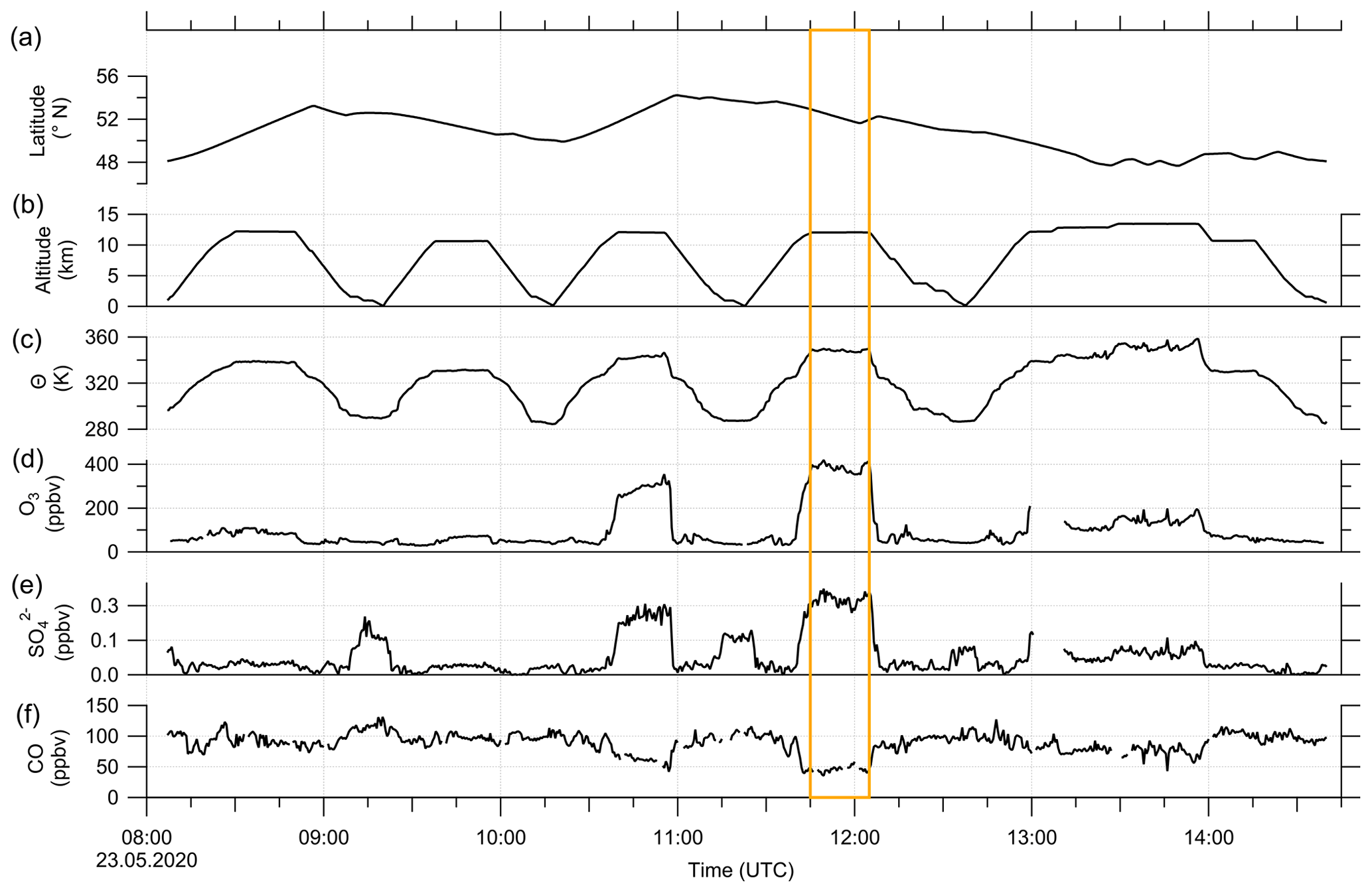
Figure 7Time series of in situ measurements during research flight RF01 on 23 May 2020 in 30 s time steps. (a) Latitude, (b) altitude, (c) potential temperature θ, (d) O3 mixing ratios, (e) sulfate aerosol mixing ratios and (f) CO mixing ratios. The orange box marks the period with the observed sulfate anomaly described in the text and shown in Fig. C1. In addition, we added a time series of all aerosol species to the Appendix (see Fig. E3).
Figure 4 reveals the correlation between CO and particulate sulfate in the lower troposphere as well as the positive correlation between particulate sulfate and O3 and the anticorrelation between sulfate and CO in the stratosphere. To identify mixing from the measurements, we use two types of scatterplots. The first is the previously introduced scatterplot using CO and O3 with different color coding (Fig. 8a–c), and the second is the scatterplot with H2O and O3 (Hegglin et al., 2009) (see Fig. 8d–f). This figure contains only data measured on 23 May 2020. The H2O–O3 method follows the same principle, with high water vapor mixing ratios in the troposphere and a constant stratospheric background value around 5 ppmv (Hegglin et al., 2009). In our dataset, the lowest observed H2O values are around 10 ppmv, indicating that we did not fully reach stratospheric background conditions. All of these scatterplots show two separate branches of mixing lines. This feature is most obvious in the H2O–O3 correlation. Here, one mixing line connects the tropopause with around H2O = 40 ppmv and O3 = 100 ppbv and the LMS with decreasing H2O (down to 10 ppmv) at O3 = 400 ppbv. This mixing line also includes the measured sulfate anomaly and was observed over northern Germany (see Figs. 7 and C4). The second mixing line is not as pronounced, starting at drier air masses with H2O = 20 ppmv and only reaching up to O3 = 200 ppbv. These observations were made later on the flight over southern Germany (see also Figs. 7 and C4).
Regardless of the type of scatterplot, we observe an increase in the particulate sulfate mixing ratio and potential temperature along the mixing line, starting at the tropopause and extending into the stratosphere (Fig. 8). In contrast, we also observe a decrease in the CO mixing ratio. This result is consistent with the assumption that tropospheric air enters the stratosphere at lower potential temperatures with lower amounts of sulfate aerosol, correspondingly higher mixing ratios of precursor gases, and higher CO. In the stratosphere, gas-to-particle conversion of OCS and SO2 will lead to an increase in particulate sulfate. In contrast to sulfate, CO will decrease during the transport into the stratosphere, by both dilution and photochemical destruction, with an atmospheric lifetime of 1 to 3 months (Seinfeld and Pandis, 2016). This is almost the same time as the calculated e-folding time of gas-to-particle conversion of SO2 to sulfate aerosol in the midlatitude LMS region (Jurkat et al., 2010).
Further evidence that the anomaly is caused by tropospheric influence is the lower O3 values and the water vapor mixing ratios. If the air masses were of stratospheric origin, we would expect O3 mixing ratios higher than 400 ppbv and a water vapor mixing ratio around 5 ppmv. Instead, we observe lower O3 mixing ratios and water vapor mixing ratios around 10–20 ppmv.
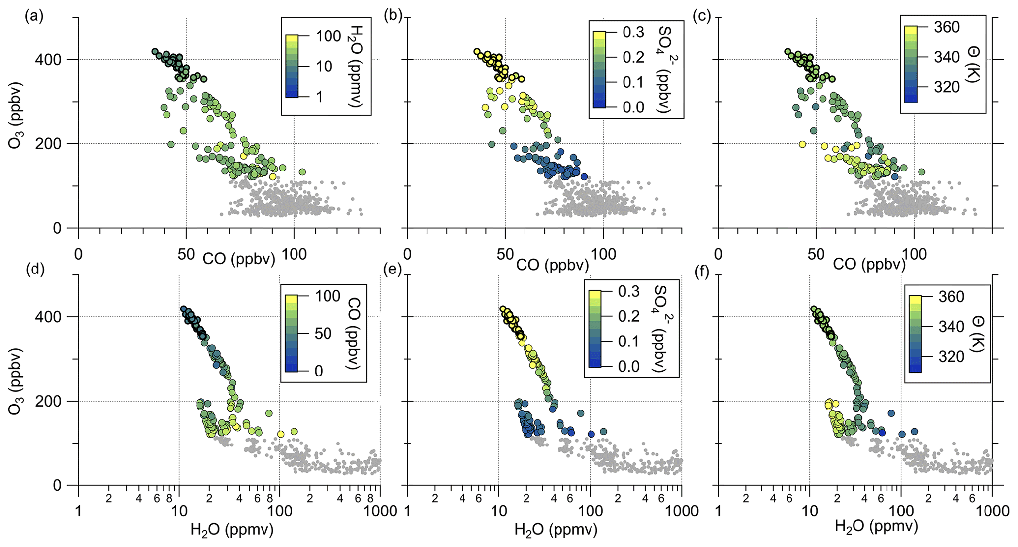
Figure 8Tracer–tracer correlations for 23 May 2020 to identify mixing processes. The CO–O3 correlations are color-coded with (a) H2O, (b) SO and (c) θ. The H2O–O3 correlations are color-coded with (d) CO, (e) SO and (f) θ. The data correspond to the blue-colored data in Fig. 3 and the sulfur anomaly in Fig. 5.
Similarly to the HALO measurements, we analyzed measurements conducted on DLR-Falcon for this analysis. DLR-Falcon performed a measurement flight on the same day and sampled in the area where the anomaly was encountered just 40 min later than HALO (Fig. C2), which allows a comparison of the measurements on both platforms with respect to dynamical processes. DLR-Falcon does not reach the same high altitudes as HALO, so the air masses were probed at lower levels and thus show higher CO mixing ratios. This time, we use the scatterplot of CO and HNO3 to identify mixing in combination with gas-to-particle conversion (Fig. 9b). HNO3 was already introduced as a stratospheric tracer by Proffitt et al. (1989) and Arnold et al. (1989) and utilized because the O3 data for DLR-Falcon are not available for this flight. Additionally, we added the measurements from HALO to this figure (Fig. 9a) to directly link them to the process of gas-to-particle conversion. We identify a mixing line in the scatterplots, connecting the troposphere and stratosphere. The HALO measurements in Fig. 9a show an increase in the total particle number concentration along the mixing line, whereas the SO2 mixing ratios on this mixing line (Fig. 9b) show a reduction with respect to the measured tropospheric maxima of 0.1 ppbv, which is an indication of gas-to-particle conversion along this mixing line. This conclusion is also supported by the correlation of the total particle number concentration with the individual species of chemical composition, measured by the C-ToF-AMS (see Fig. E5). Here we can see that the particles forming and growing are mainly sulfate aerosol particles, and the particles do not have a pure tropospheric composition. The process of gas-to-particle conversion requires a source of high mixing ratios of precursor gases, in this case SO2. In addition, due to the high solubility of SO2, it requires a very fast and mostly dry process for transport into the UTLS. One possible process that fulfills these conditions is volcanic eruptions, which leads to the assumption that the observed sulfate aerosol particles are most likely formed by volcanic influence.
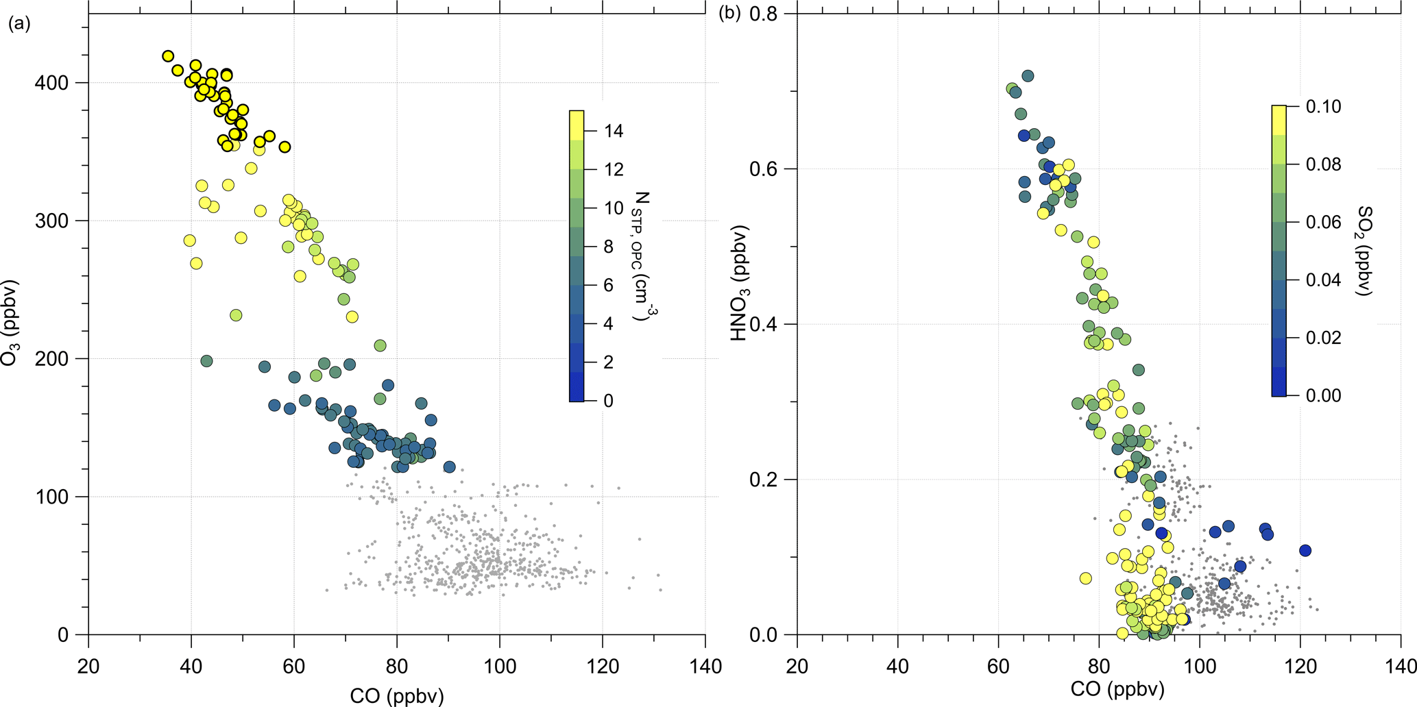
Figure 9Scatterplot of CO and O3 measured on HALO (a) and CO and HNO3 measured on DLR-Falcon (b) for the investigated flight on 23 May 2020. In panel (a) the color code shows the total particle number concentration by the OPC. For the DLR-Falcon measurements in panel (b), we color-coded with the SO2 mixing ratio. Both measurement platforms observe a mixing line in the probed area. Whereas the total aerosol number concentration is increasing along this mixing line, the SO2 measurements show a reduction. This is one possible indicator for the process of gas-to-particle conversion.
As a complement to the measurement data, we analyzed the meteorological situation along the flight path for the period of the anomaly (Fig. B1). The flight path was located just above the maximum of the subtropical jet stream and a layer of strong vertical wind shear (Fig. B1a). Further, we see that the flight path crossed a layer of a low-gradient Richardson number (Fig. B1b) and later continued slightly above this layer. This indicated a region of instability which is an important factor in mixing processes.
The previous discussion has shown that mixing between tropospheric and stratospheric air masses most likely occurred before and during the in situ measurements.
Hereafter, we examine the origin of the air masses comprised of high mixing ratios of sulfate aerosol. Therefore, we exploit LAGRANTO back trajectories, starting at a grid around the flight path with 230 trajectories for each measurement point. The trajectories are calculated 10 d backward to see whether the air masses show any fresh influence from the troposphere or a rather stable flow within the lowermost stratosphere. For our analysis, we filtered the trajectories by selecting only those with a minimum potential temperature below 345 K and with an increase of at least 5 K potential temperature. Figure 10 shows that the selected trajectories are close together and move with the jet stream. The trajectories crossed the region of East Asia within 10 d before the measurement, and most of them crossed China and its megacities like Chengdu and Shanghai. The time series of potential temperature shows that no boundary layer air masses were transported to the measurement region in the last 10 d (Fig. 10a), considering the assumption that the trajectories can resolve convective uplift. As a consequence, the enhanced particulate sulfate needs to be older than 10 d and was most likely not directly mixed into the LMS as particulate sulfate, and this also supports the findings in the previous analysis (see, e.g., Figs. 9 and E5).
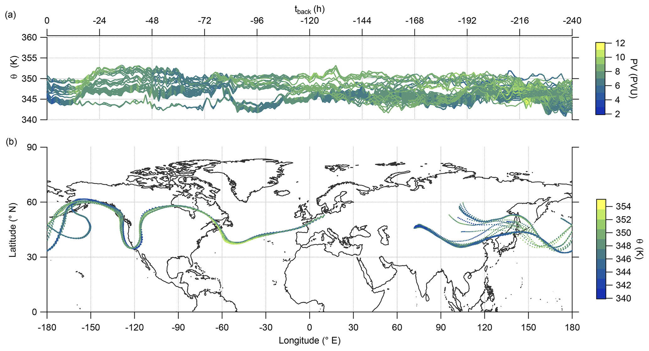
Figure 10LAGRANTO 10 d back trajectories for cases with enhanced SO in the lowermost stratosphere. The upper panel (a) shows a time series of θ color-coded with PV. The lower panel (b) shows the position of the trajectories on the map with θ as the color code.
Alternatively, the sulfate aerosol, as mentioned earlier, could originate from gas-to-particle conversion of SO2 that was mixed into the LMS. To examine this hypothesis, we start from Fig. 9, which shows that, close to the tropopause, the SO2 values are quite high and decrease along the mixing line, whereas the aerosol total number concentration increases. This is an indicator of ongoing gas-to-particle conversion in combination with cross-tropopause mixing. To confirm this possible process, it needs a strong source of SO2 which is strong enough to transport the SO2 in a short time to high altitudes with as few as possible moist processes to not wash it out from the atmosphere. One possible source of such a process could be volcanic activities. Therefore, we searched for volcanic eruptions in the period of 2 months before the measurements, corresponding to the e-folding time of about 50 to 60 d (Jurkat et al., 2010). For the analysis, we used volcanic eruption databases in combination with daily TROPOspheric Monitoring Instrument (TROPOMI) retrievals in different volcanically active regions to identify possible source regions. Thereby, we identified the Kamchatka Peninsula in Russia as an origin of enhanced SO2 emissions in the beginning of April 2020. This corresponds to the archived reports by the Kamchatka Volcanic Eruption Response Team (KVERT) (Institute of Volcanology and Seismology FEB RAS, 2023). In the report for 8 April 2020, an explosive eruption of the Sheveluch volcano is described, with a volcanic cloud height reaching up to 10 km and thus into the tropopause region. We performed HYSPLIT (Stein et al., 2015) forward-dispersion simulations of the Sheveluch volcano plume and analyzed the eruption plume in the model at different heights to get a broad overview of the distribution. Therefore, we calculated forward trajectories at heights between 9000 and 11 000 m with a vertical resolution of 500 m. In the following, we only consider the levels up to 9000 m (see Fig. D1) and between 10 000 and 11 000 m (see Fig. 11), because here the model shows differences in the plume and indicates possible mixing into the stratosphere.
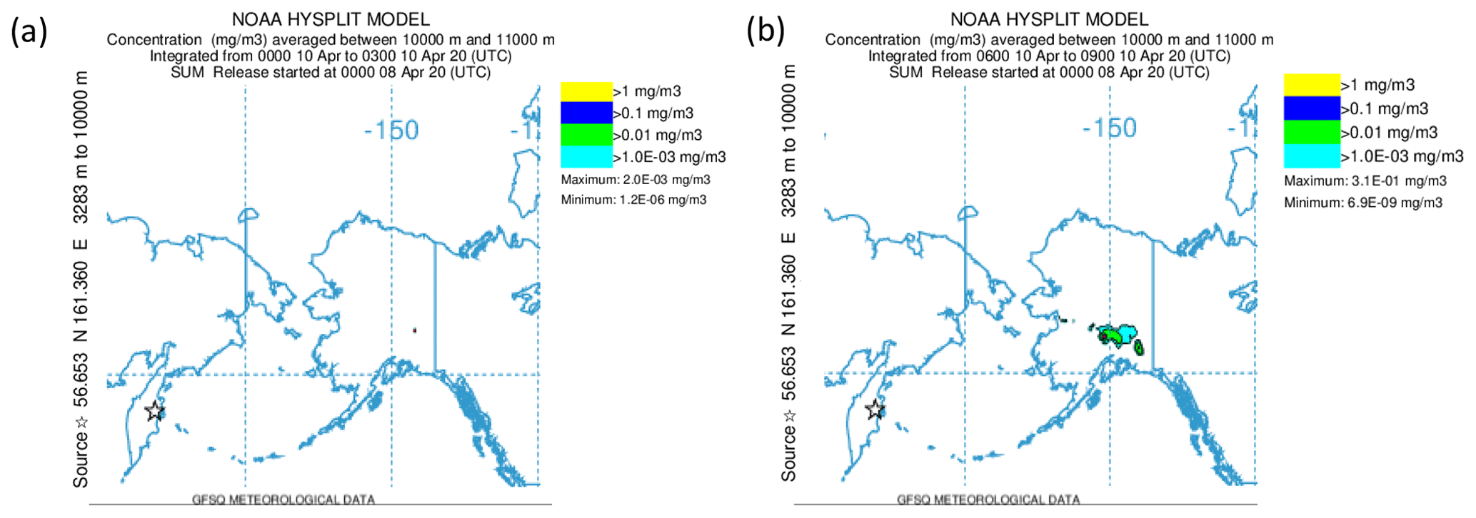
Figure 11NOAA HYSPLIT dispersion model simulation (Stein et al., 2015) for the Sheveluch eruption on 8 April 2020 on the basis of GFS meteorological data. The particle concentration between 10 000 and 11 000 m is depicted. Panel (a) shows the averaging period on 10 April 2020 from 00:00 until 03:00 UTC, and panel (b) shows the next period on 10 April 2020 from 06:00 until 09:00 UTC.
We observe a large volcanic plume up to 9000 m which is distributed, spread and stretched within the first 3 d over the North Pacific, reaching over Alaska and also eastwards, close to the Hudson Bay, Canada (see Fig. D1). For the layer between 10 000 and 11 000 m, the results look completely different (see Fig. 11). Here, we observe no signal of the volcanic plume on the first day. However, more areas with volcanic plume influence occur over Alaska, reaching towards Canada during the second day. These affected areas increase over time. Thus, the HYSPLIT dispersion model results also support the hypothesis of mixing volcanic emissions into the stratosphere within the first 3 d. This is an additional indicator of the mixing of SO2 into the stratosphere, resulting in higher SO2 mixing ratios compared to the background. After the mixing of SO2 into the LMS, the process of gas-to-particle conversion starts and forms particulate sulfate aerosol over several weeks. This results in the observation of higher mixing ratios of particulate sulfate in the LMS roughly 7 weeks after the eruption, especially for research flight RF01, where the flight path was close to the jet stream and crossed one filament of volcanically influenced air masses.
Usually, trace gas correlations, such as CO–O3 or H2O–O3, have been used to study mixing processes between the troposphere and stratosphere. In our study, we showed that, in addition to trace gas measurements, aerosol measurements, especially particulate sulfate, can also be applied to identify troposphere–stratosphere exchange. Furthermore, we showed that the method to define the chemical tropopause proposed by Zahn et al. (2004) is in agreement with the dynamical tropopause definition for our campaign and is thus suitable for the separation of stratospheric and tropospheric air masses. Similar to the correlation between CO and O3, the correlation of SO and O3 in the lowermost stratosphere also showed some variability induced by mixing events. In a case study during the CAFE-EU/BLUESKY mission, we observed air masses with high sulfate mixing ratios in the lowermost stratosphere, reaching values that are typically found at higher altitudes in the stratospheric aerosol layer. Meteorological and dynamical parameters such as vertical wind shear and gradient Richardson number indicated that mixing across the tropopause occurred in this region and along the transport and air mass history. Additionally, we found that this anomaly of higher particulate sulfate in the lowermost stratosphere occurred during one single flight. During this flight, we found one mixing line in the CO–O3 correlation with increasing sulfate aerosol mixing ratios and total aerosol number concentration towards the stratosphere. In addition, we used measurements of the quasi co-located DLR-Falcon aircraft. In the same tracer–tracer correlation framework, using HNO3 instead of O3, we also found one mixing line. In contrast to the increasing sulfate aerosol for the HALO measurements, we observed decreasing mixing ratios of SO2, which is a precursor gas for particulate sulfate. The combination of the sulfate aerosol mixing ratio, the total aerosol number concentration as well as the reduction in SO2 in the same measurement region led to the hypothesis of upward mixing of precursor gases and ongoing gas-to-particle conversion in the lowermost stratosphere. Here, we could identify volcanic activities on the Kamchatka Peninsula, Russia, and the explosive eruption of the Sheveluch volcano as a possible source of the SO2 in the tropopause region. The Sheveluch eruption injected SO2 directly into the upper troposphere, from where it was mixed into the stratosphere, with subsequent gas-to-particle conversion to sulfate aerosol. We can thus conclude that the chemical composition of the aerosol in the lowermost stratosphere is affected by small-scale mixing processes and that the ExTL can thus also be characterized by aerosol properties. In addition to direct mixing of aerosol particles, the process of mixing of precursor gases with subsequent gas-to-particle conversion also needs to be considered, as we showed in our case study. We intend to use this method in the future with data obtained during previous airborne measurements in the UTLS to extend the analysis to a larger scale. Furthermore, we aim to compare the results with chemistry climate model studies to see whether chemical transport models can represent small-scale mixing across the tropopause and the associated gas-to-particle conversion processes. Another study should investigate how models represent the influence of volcanic eruptions on the lowermost stratosphere.
In the following, we explain the adjustment of our bin scheme for the two-dimensional binning analysis. Figure A1b shows the data distribution for the evenly distributed bin scheme in the vertical. Here, we see that many bins in the LMS contain less than 10 data points, so we could expect some bias in the median. Therefore, we enlarge the vertical bins at 350 K and above to 10 K to include more data points in one vertical bin and increase the statistic of the analysis without losing information.
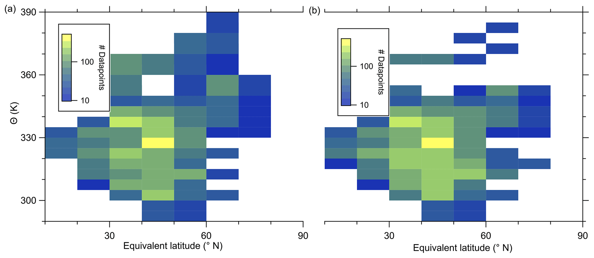
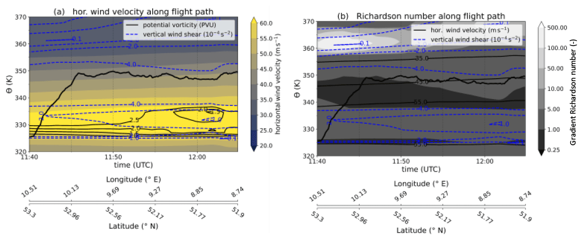
Figure B1Meteorological cross sections along the flight path, calculated on the basis of ERA5 reanalysis data (Hersbach et al., 2020). Panel (a) contains the horizontal wind speed as a filled contour, the flight altitude as a black bold solid line, the PV contour as thin black lines and the vertical wind shear as dashed blue contour lines. In panel (b) the filled contour changed to the gradient Richardson number, and the thin black lines are contour lines of the horizontal wind speed. Latitude and longitude values are added to the time series for reference.
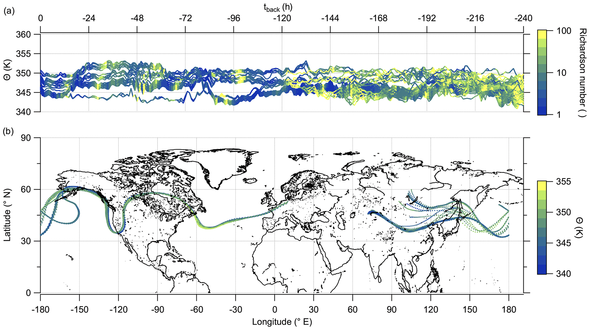
Figure B2LAGRANTO 10 d back trajectories for cases with enhanced SO in the lowermost stratosphere starting in northern Germany. (a) Time series of θ color-coded with the gradient Richardson number as a marker for potentially instable regions along the trajectories. (b) The position of the trajectories on the map and the potential temperature as a color code.
This section offers some meteorological analysis for the flight segment with the observed particulate sulfate anomaly (see Fig. B1). Afterwards, we show some additional data along the back trajectories. More precisely, we show the time series of the Richardson number to indicate potential instable regions the air masses have crossed before the measurement (see Fig. B2). First we want to introduce the used variables for our stability analysis, similar to, e.g., Kaluza et al. (2019) or Kunkel et al. (2019):
Turbulence may occur at a gradient Richardson number lower than 0.25.
The following figures are supporting information on the observed anomaly of higher mixing ratios of particulate sulfate. This includes a detailed view of research flight RF01, where the anomaly was observed (Fig. C1). Figure C2 locates the flight segment of the anomaly on the map, including the quasi co-located DLR-Falcon flight path and the sulfur dioxide mixing ratio measured on DLR-Falcon. The last figure (Fig. C3) highlights two selected research flights and their corresponding accuracy within the correlation of the complete dataset.
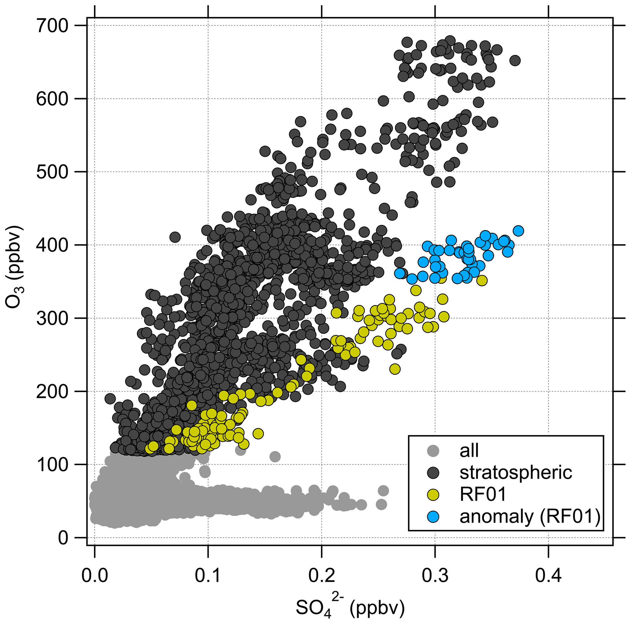
Figure C1Scatterplot of the in situ measured SO and O3 containing or including all the campaign data in bright grey. Stratospheric data points are colored in dark grey. The mixing event of research flight RF01 is indicated in yellow and the sulfate anomaly identified during this flight in blue.
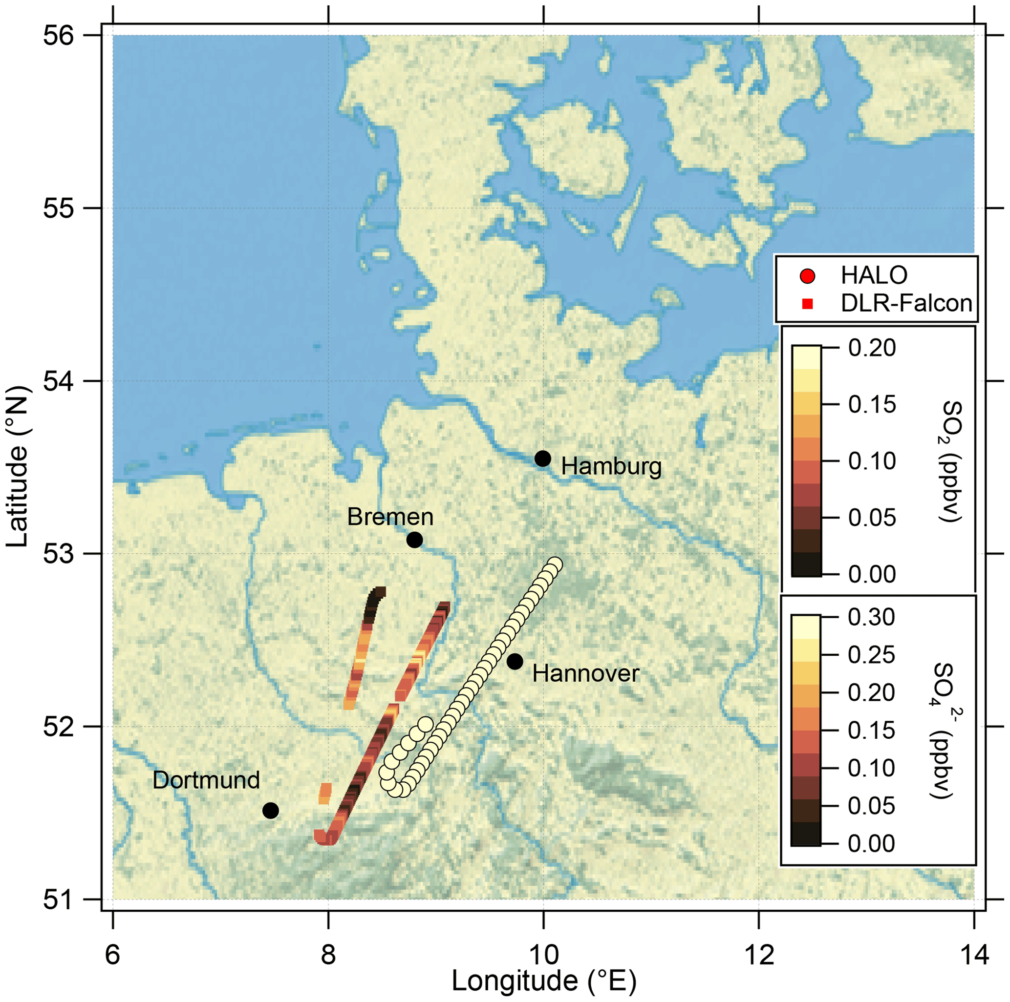
Figure C2Location of the analyzed flight segment during the research flight on 23 May 2020 between 11:45 and 12:05 UTC, where the mixing event in the vicinity of the jet stream was observed. The flight path of HALO is shown with the filled circles color-coded with the sulfate mixing ratio, and the flight path of DLR-Falcon is shown with the filled squares color-coded with the SO2 mixing ratio. The map was created from public-domain GIS data found on the Natural Earth website (http://www.naturalearthdata.com, last access: 2 January 2024).
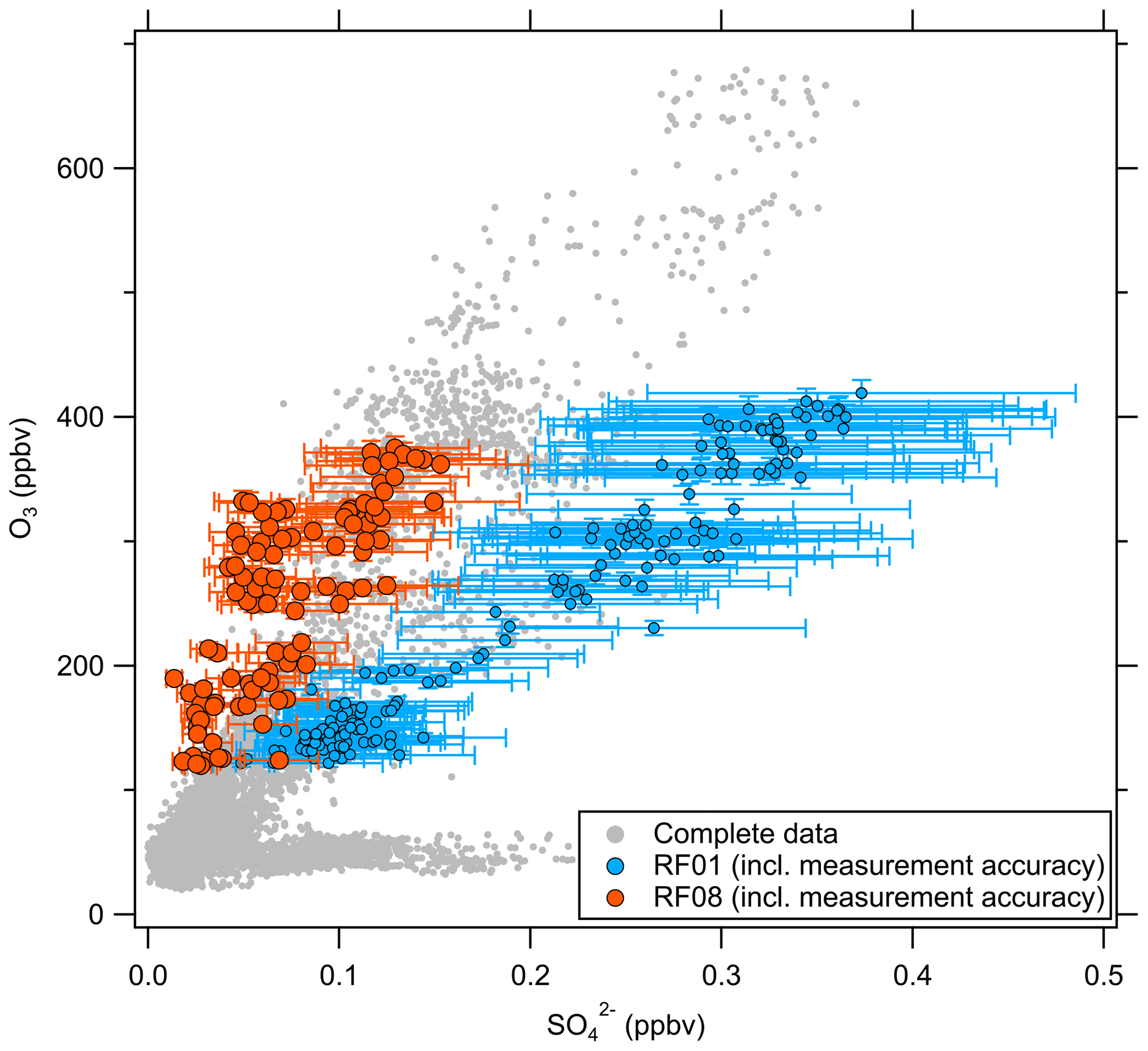
Figure C3Scatterplot of particulate sulfate against O3 for the complete campaign dataset. The data points for flights RF01 and RF08 are highlighted together with their measurement accuracy as examples.
The following maps (Fig. C4) of the measured stratospheric air during RF01 help to interpret both mixing lines found in Fig. 8. Herewith, we can differentiate between the measured elevated particulate sulfate over northern Germany and the more subtropical air over southern Germany with respect to their characteristics.
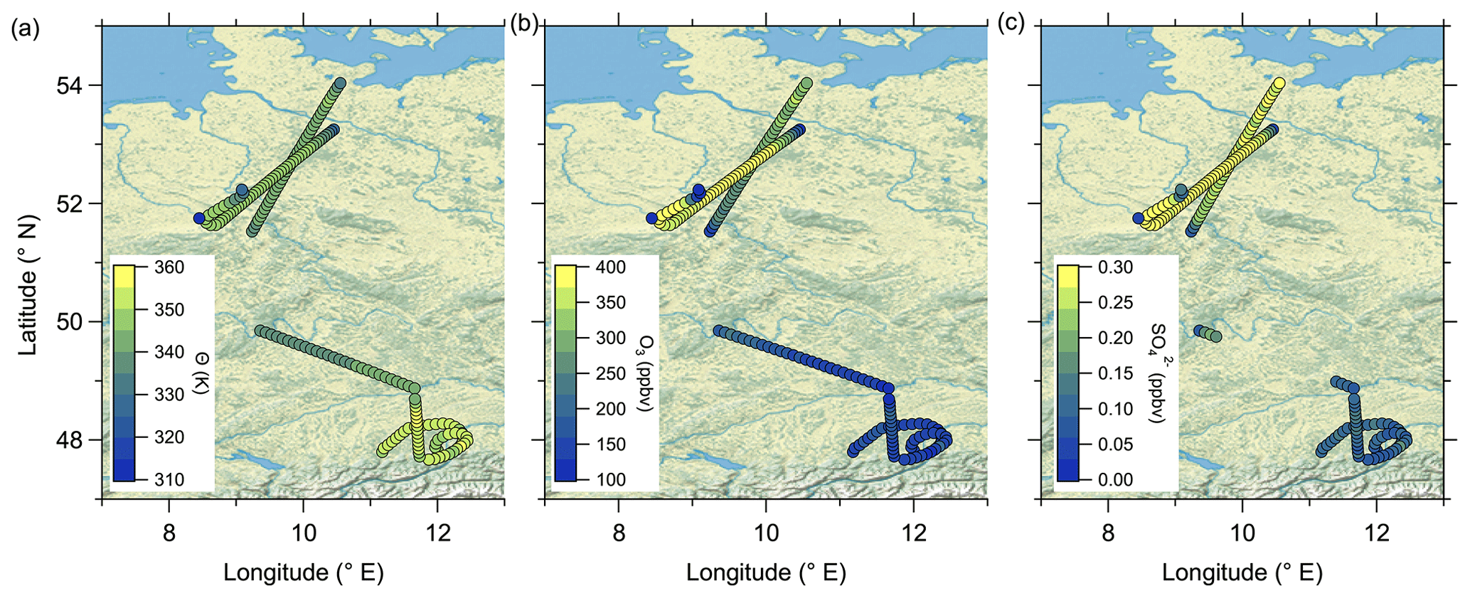
Figure C4The stratospheric flight segments of RF01 on 23 May 2020 are shown and color-coded with (a) potential temperature θ, (b) O3 mixing ratios and (c) particulate sulfate mixing ratios. The map was created from public-domain GIS data found on the Natural Earth website (http://www.naturalearthdata.com, last access: 2 January 2024).
The figure shown in this section is in addition to Fig. 11 and shows similar variables but for the altitude range from sea level up to 9000 m to show the entire volcanic main plume and its distribution.
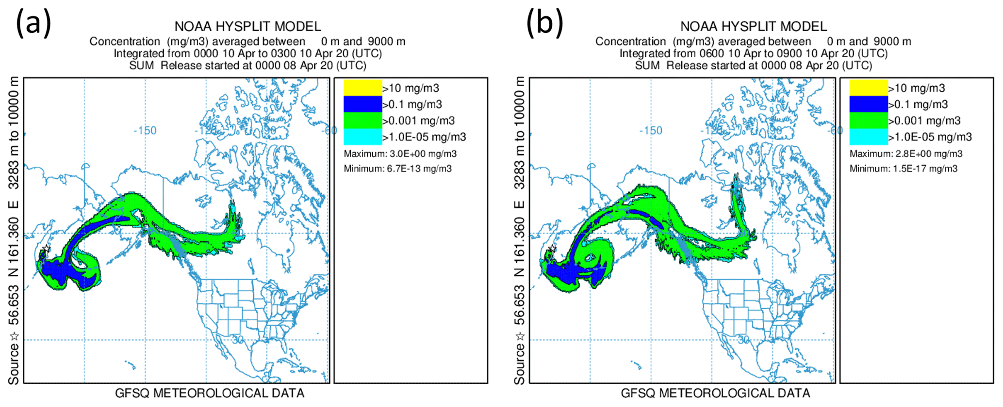
Figure D1NOAA HYSPLIT dispersion model simulation for the Sheveluch eruption on 8 April 2020 on the basis of GFS meteorological data (Stein et al., 2015). The location of the Sheveluch volcano is given by a little star. Further, the particle concentration averaged between sea level and 9000 m is shown. Panel (a) includes the averaging period on 10 April 2020 from 00:00 to 03:00 UTC, and panel (b) shows the next period on the same day from 06:00 to 09:00 UTC.
This section gives an overview of the complete dataset produced by the C-ToF-AMS in combination with the OPC that is integrated into the instrument system. In the following, we show vertical profiles of the aerosol species measured by the AMS relative to the potential temperature and the geometric altitude to support the anomalous observation of the sulfate concentration described in the case study.
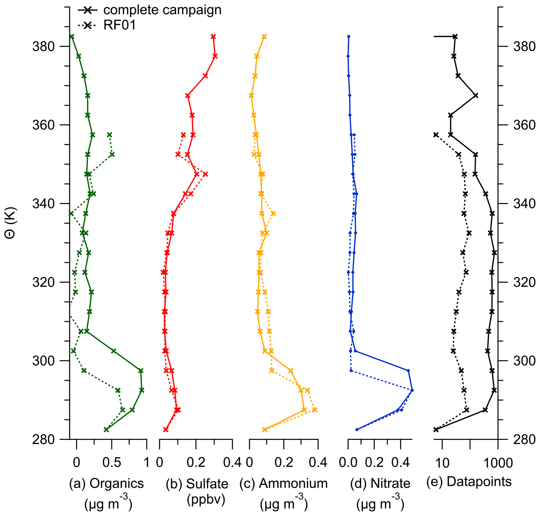
Figure E1Binned vertical profiles for 5 K potential temperature bins for all species measured by the C-ToF-AMS: (a) organic aerosol, (b) sulfate aerosol, (c) ammonium aerosol and (d) nitrate aerosol. The number of data points for each bin is shown in panel (e). The vertical profiles are divided into the complete dataset (solid lines) and data only from case study RF01 (dotted lines).
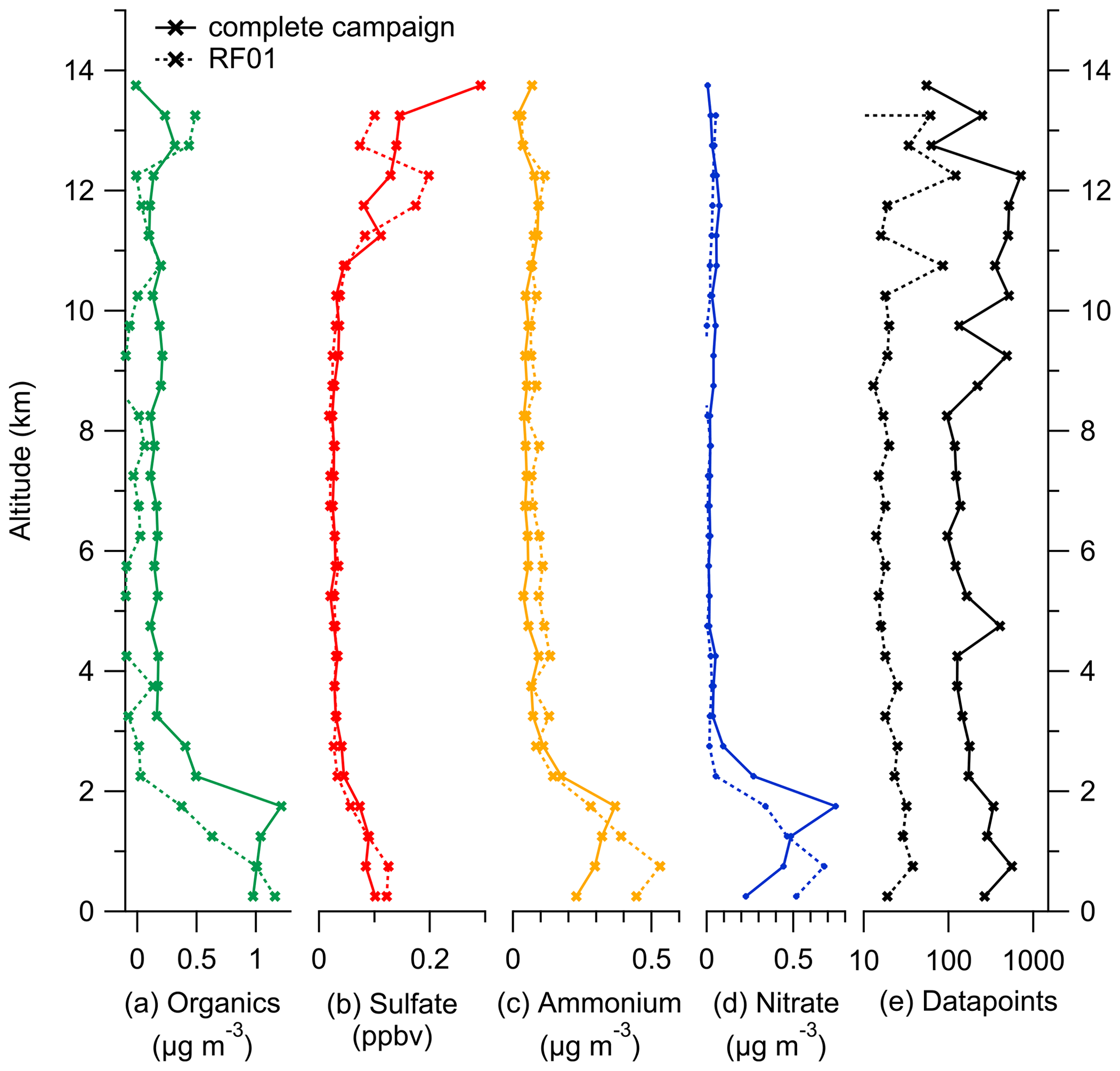
Figure E2Binned vertical profiles for 500 m altitude bins for all species measured by the C-ToF-AMS: (a) organic aerosol, (b) sulfate aerosol, (c) ammonium aerosol and (d) nitrate aerosol. The number of data points for each bin is shown in panel (e). The vertical profiles are divided into the complete dataset (solid lines) and data only from case study RF01 (dotted lines).
The following plot shows the time series of the altitude and the aerosol measurements conducted by the C-ToF-AMS during RF01. The orange box indicates the time period when the sulfate anomaly was observed. Further, the different chemical composition of the probed air masses is visible, similar to the described characteristics in Figs. C4 and 7.
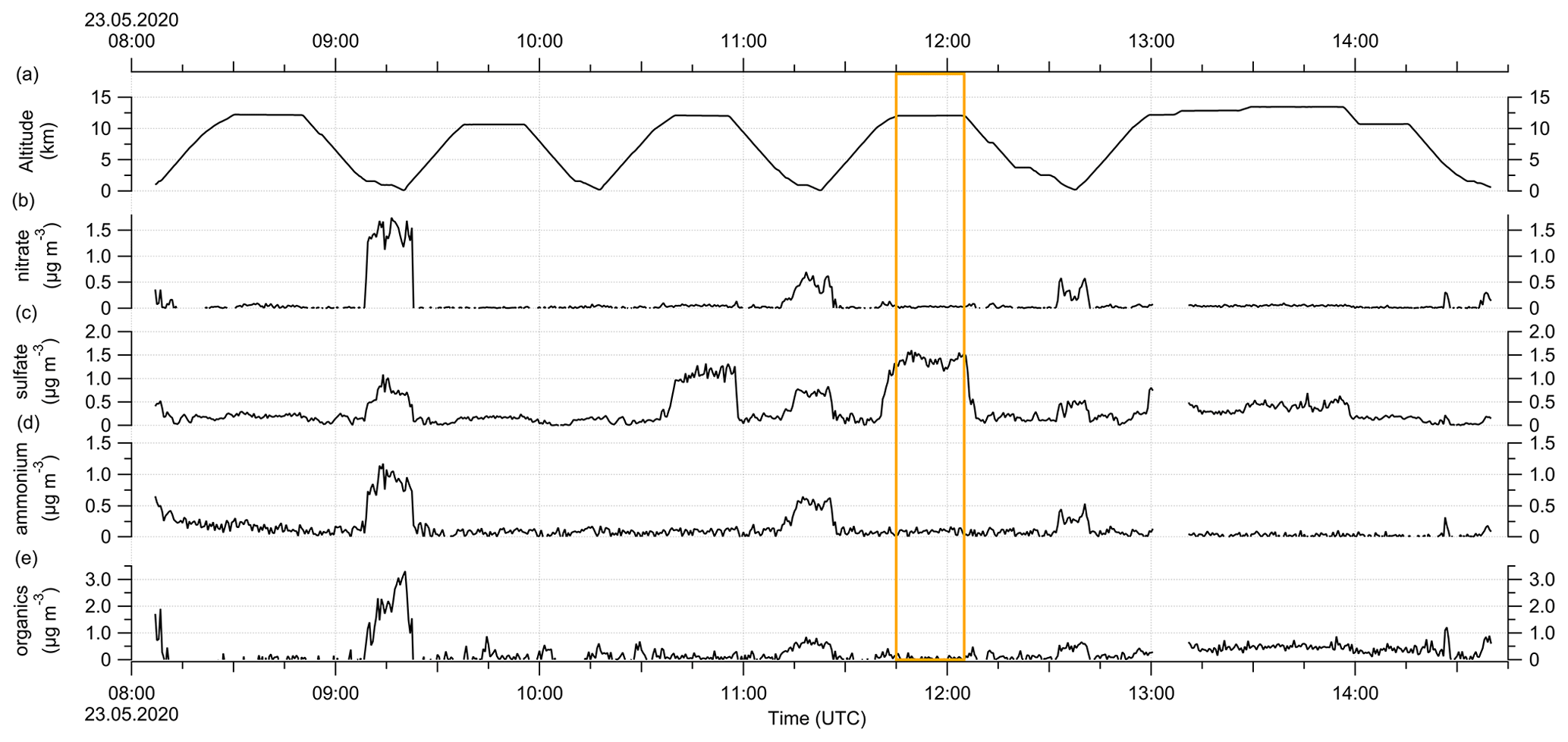
Figure E3Time series of the aerosol measurements during RF01 on 23 May 2020 in 30 s time steps. (a) Altitude, (b) nitrate aerosol, (c) sulfate aerosol, (d) ammonium aerosol and (e) organic aerosol mass concentration. The orange box marks the period with the observed sulfate anomaly described in the text and shown in Fig. C1.
In addition to the chemical composition analysis, we looked at the aerosol size distribution and number concentration measured by the OPC. Therefore, we compare different stratospheric measurement periods. In Fig. E4, we show the size distribution corresponding to the 20 min of the sulfate anomaly and compare it with 20 min measurements for the stratospheric part over southern Germany under background conditions. During the anomaly, we observe up to 2 times more particles within the individual size bins below 1 µm.
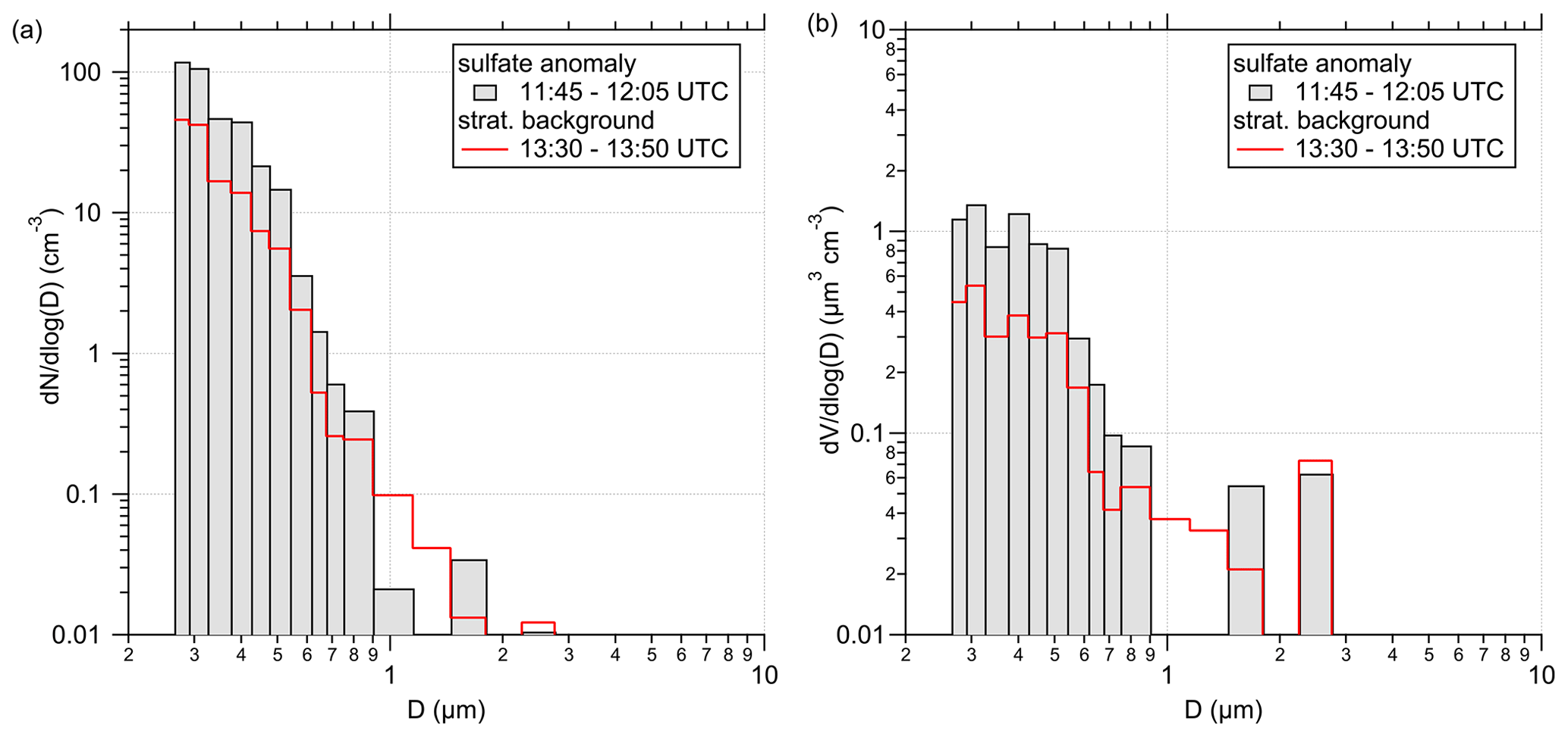
Figure E4Size (a) and volume distribution (b), STP-corrected and measured by the OPC. The distributions are averaged over a 20 min time period for two different measurement regimes. One is the described sulfate anomaly (grey-filled bars), and the other is a time period of the stratospheric background (red lines) later during this flight as a comparison.
To illustrate the chemical composition of the formed particles in Fig. 9a, we correlate the total number concentration N with the individual aerosol species in the next figure.
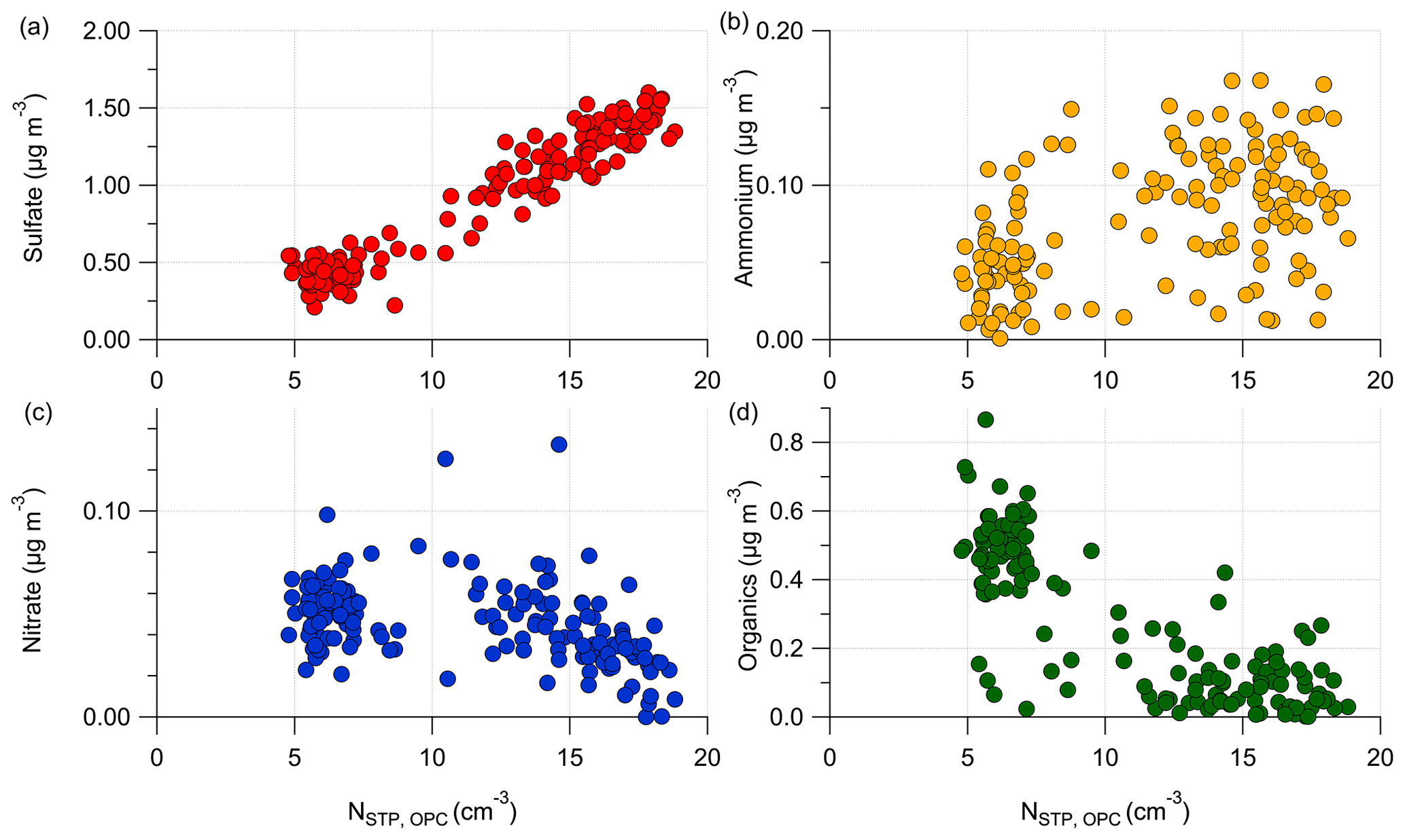
Figure E5Correlation of the total aerosol number concentration N, STP-corrected and measured by the OPC with the aerosol species measured by the C-ToF-AMS: (a) with particulate sulfate, (b) with ammonium, (c) with nitrate and (d) with organic aerosol. The shown data represent the stratospheric measurements during RF01.
Data measured on board HALO are available on request from the HALO database at https://halo-db.pa.op.dlr.de/mission/120 (HALO, 2024a). The DLR-Falcon basic aircraft data and the AIMS data are available on request from the HALO database at https://halo-db.pa.op.dlr.de/mission/119 (HALO, 2024b) or on request to the authors. The trajectories are published on Zenodo (Kunkel and Joppe, 2024) (https://doi.org/10.5281/ZENODO.11092106).
PJ set up the study together with JS, performed the data analysis and prepared the manuscript. KK and JS provided the AMS and OPC data and supported the analysis. LT, AM and CV provided the SO2 and HNO3 data. HS provided CO and O3 data from DLR-Falcon. AZ provided the O3 data from HALO. HF and LR provided CO data from HALO. HCL and DK provided model data and back trajectories as well as the code for the cross sections along the flight path. All the co-authors commented on the manuscript and discussed the presented results.
The contact author has declared that none of the authors has any competing interests.
Publisher’s note: Copernicus Publications remains neutral with regard to jurisdictional claims made in the text, published maps, institutional affiliations, or any other geographical representation in this paper. While Copernicus Publications makes every effort to include appropriate place names, the final responsibility lies with the authors.
Philipp Joppe is funded by the Deutsche Forschungsgemeinschaft (DFG, German Research Foundation) – TRR 301 – project ID 428312742, “The tropopause region in a changing atmosphere”, subproject A04 coordinated by Johannes Schneider, Stephan Borrmann and Franziska Köllner. Laura Tomsche and Christiane Voigt are also funded by the TRR 301 – project ID 428312742 in subproject A01. The HALO measurement flights during CAFE-EU/BLUESKY were funded by the Max Planck Society. The authors thank the DLR team for making a campaign possible during the COVID-19 lockdown in Germany.
The authors thank the NOAA Air Resources Laboratory for providing the HYSPLIT dispersion calculations on their website.
This research has been supported by the Deutsche Forschungsgemeinschaft (grant no. 428312742).
The article processing charges for this open-access publication were covered by the Max Planck Society.
This paper was edited by Eduardo Landulfo and reviewed by two anonymous referees.
Andreae, M. O.: Ocean-atmosphere interactions in the global biogeochemical sulfur cycle, Mar. Chem., 30, 1–29, https://doi.org/10.1016/0304-4203(90)90059-l, 1990. a
Appel, O., Köllner, F., Dragoneas, A., Hünig, A., Molleker, S., Schlager, H., Mahnke, C., Weigel, R., Port, M., Schulz, C., Drewnick, F., Vogel, B., Stroh, F., and Borrmann, S.: Chemical analysis of the Asian tropopause aerosol layer (ATAL) with emphasis on secondary aerosol particles using aircraft-based in situ aerosol mass spectrometry, Atmos. Chem. Phys., 22, 13607–13630, https://doi.org/10.5194/acp-22-13607-2022, 2022. a
Arnold, F., Schlager, H., Hoffmann, J., Metzinger, P., and Spreng, S.: Evidence for stratospheric nitric acid condensation from balloon and rocket measurements in the Arctic, Nature, 342, 493–497, 1989. a
Bahreini, R., Ervens, B., Middlebrook, A. M., Warneke, C., de Gouw, J. A., DeCarlo, P. F., Jimenez, J. L., Brock, C. A., Neuman, J. A., Ryerson, T. B., Stark, H., Atlas, E., Brioude, J., Fried, A., Holloway, J. S., Peischl, J., Richter, D., Walega, J., Weibring, P., Wollny, A. G., and Fehsenfeld, F. C.: Organic aerosol formation in urban and industrial plumes near Houston and Dallas, Texas, J. Geophys. Res.-Atmos., 114, D00F16 , https://doi.org/10.1029/2008jd011493, 2009. a, b
Barré, J., El Amraoui, L., Ricaud, P., Lahoz, W. A., Attié, J.-L., Peuch, V.-H., Josse, B., and Marécal, V.: Diagnosing the transition layer at extratropical latitudes using MLS O3 and MOPITT CO analyses, Atmos. Chem. Phys., 13, 7225–7240, https://doi.org/10.5194/acp-13-7225-2013, 2013. a
Bethan, S., Vaughan, G., and Reid, S. J.: A comparison of ozone and thermal tropopause heights and the impact of tropopause definition on quantifying the ozone content of the troposphere, Q. J. Roy. Meteorol. Soc., 122, 929–944, https://doi.org/10.1002/qj.49712253207, 1996. a
Bönisch, H., Engel, A., Curtius, J., Birner, Th., and Hoor, P.: Quantifying transport into the lowermost stratosphere using simultaneous in-situ measurements of SF6 and CO2, Atmos. Chem. Phys., 9, 5905–5919, https://doi.org/10.5194/acp-9-5905-2009, 2009. a
Borrmann, S., Dye, J. E., Baumgardner, D., Wilson, J. C., Jonsson, H. H., Brock, C. A., Loewenstein, M., Podolske, J. R., Ferry, G. V., and Barr, K. S.: In-situ measurements of changes in stratospheric aerosol and the N2O-aerosol relationship inside and outside of the polar vortex, Geophys. Res. Lett., 20, 2559–2562, https://doi.org/10.1029/93gl01694, 1993. a, b
Borrmann, S., Dye, J. E., Baumgardner, D., Proffitt, M. H., Margitan, J. J., Wilson, J. C., Jonsson, H. H., Brock, C. A., Loewenstein, M., Podolske, J. R., and Ferry, G. V.: Aerosols as dynamical tracers in the lower stratosphere: Ozone versus aerosol correlation after the Mount Pinatubo eruption, J. Geophys. Res.-Atmos., 100, 11147–11156, https://doi.org/10.1029/95jd00016, 1995. a, b, c
Brimblecombe, P.: The Global Sulfur Cycle, 559–591 p., Elsevier, https://doi.org/10.1016/b978-0-08-095975-7.00814-7, 2014. a
Brühl, C., Lelieveld, J., Crutzen, P. J., and Tost, H.: The role of carbonyl sulphide as a source of stratospheric sulphate aerosol and its impact on climate, Atmos. Chem. Phys., 12, 1239–1253, https://doi.org/10.5194/acp-12-1239-2012, 2012. a, b, c
Butchart, N. and Remsberg, E. E.: The Area of the Stratospheric Polar Vortex as a Diagnostic for Tracer Transport on an Isentropic Surface, J. Atmos. Sci., 43, 1319–1339, https://doi.org/10.1175/1520-0469(1986)043<1319:taotsp>2.0.co;2, 1986. a
Canagaratna, M. R., Canagaratna, M. R., Jayne, J. T., Jimenez, J. L., Allan, J., Alfarra, M. R., Alfarra, M. R., Zhang, Q., Zhang, Q., Zhang, Q., Onasch, T. B., Onasch, T. B., Drewnick, F., Coe, H., Middlebrook, A. M., Delia, A. E., Williams, L. R., Trimborn, A., Northway, M. J., Northway, M. J., DeCarlo, P. F., Kolb, C. E., Davidovits, P., and Worsnop, D. R.: Chemical and microphysical characterization of ambient aerosols with the aerodyne aerosol mass spectrometer, Mass Spectro. Rev., 26, 185–222, https://doi.org/10.1002/mas.20115, 2007. a
Crutzen, P. J.: The possible importance of CSO for the sulfate layer of the stratosphere, Geophys. Res. Lett., 3, 73–76, https://doi.org/10.1029/GL003i002p00073, 1976. a
Deshler, T.: A review of global stratospheric aerosol: Measurements, importance, life cycle, and local stratospheric aerosol, Atmos. Res., 90, 223–232, https://doi.org/10.1016/j.atmosres.2008.03.016, 2008. a
Drewnick, F., Hings, S. S., DeCarlo, P. F., Jayne, J. T., Gonin, M., Fuhrer, K., Weimer, S., Jimenez, J. L., Demerjian, K. L., Borrmann, S., Borrmann, S., and Worsnop, D. R.: A New Time-of-Flight Aerosol Mass Spectrometer (TOF-AMS) – Instrument Description and First Field Deployment, Aerosol Sci. Technol., 39, 637–658, https://doi.org/10.1080/02786820500182040, 2005. a
Fadnavis, S., Semeniuk, K., Pozzoli, L., Schultz, M. G., Ghude, S. D., Das, S., and Kakatkar, R.: Transport of aerosols into the UTLS and their impact on the Asian monsoon region as seen in a global model simulation, Atmos. Chem. Phys., 13, 8771–8786, https://doi.org/10.5194/acp-13-8771-2013, 2013. a
Feinberg, A., Sukhodolov, T., Luo, B.-P., Rozanov, E., Winkel, L. H. E., Peter, T., and Stenke, A.: Improved tropospheric and stratospheric sulfur cycle in the aerosol–chemistry–climate model SOCOL-AERv2, Geosci. Model Dev., 12, 3863–3887, https://doi.org/10.5194/gmd-12-3863-2019, 2019. a
Fischer, H., Wienhold, F. G., Hoor, P., Bujok, O., Schiller, C., Siegmund, P., Ambaum, M., Scheeren, H. A., and Lelieveld, J.: Tracer correlations in the northern high latitude lowermost stratosphere: Influence of cross-tropopause mass exchange, Geophys. Res. Lett., 27, 97–100, https://doi.org/10.1029/1999GL010879, 2000. a, b
Friberg, J., Martinsson, B. G., Andersson, S. M., Brenninkmeijer, C. A. M., Hermann, M., Van Velthoven, P. F. J., and Zahn, A.: Sources of increase in lowermost stratospheric sulphurous and carbonaceous aerosol background concentrations during 1999–2008 derived from CARIBIC flights, Tellus B, 66, 23428, https://doi.org/10.3402/tellusb.v66.23428, 2014. a
Friberg, J., Martinsson, B. G., Andersson, S. M., and Sandvik, O. S.: Volcanic impact on the climate – the stratospheric aerosol load in the period 2006–2015, Atmos. Chem. Phys., 18, 11149–11169, https://doi.org/10.5194/acp-18-11149-2018, 2018. a
Froyd, K. D., Murphy, D. M., Sanford, T. J., Thomson, D. S., Wilson, J. C., Pfister, L., and Lait, L.: Aerosol composition of the tropical upper troposphere, Atmos. Chem. Phys., 9, 4363–4385, https://doi.org/10.5194/acp-9-4363-2009, 2009. a
Gettelman, A., Hoor, P., Pan, L. L., Randel, W. J., Hegglin, M. I., and Birner, T.: THE EXTRATROPICAL UPPER TROPOSPHERE AND LOWER STRATOSPHERE, Rev. Geophys., 49, RG3003, https://doi.org/10.1029/2011RG000355, 2011. a, b
Gorkavyi, N., Krotkov, N., Li, C., Lait, L., Colarco, P., Carn, S., DeLand, M., Newman, P., Schoeberl, M., Taha, G., Torres, O., Vasilkov, A., and Joiner, J.: Tracking aerosols and SO2 clouds from the Raikoke eruption: 3D view from satellite observations, Atmos. Meas. Tech., 14, 7545–7563, https://doi.org/10.5194/amt-14-7545-2021, 2021. a
HALO: HALO: Mission: CAFE-EU, HALO [data set], https://halo-db.pa.op.dlr.de/mission/120 (last access: 26 June 2024), 2024a. a
HALO: Mission: BLUESKY, HALO [data set], https://halo-db.pa.op.dlr.de/mission/119 (last access: 26 June 2024), 2024b. a
Hegglin, M. I.: Determination of eddy diffusivity in the lowermost stratosphere, Geophys. Res. Lett., 32, L13812, https://doi.org/10.1029/2005gl022495, 2005. a
Hegglin, M. I., Brunner, D., Peter, T., Hoor, P., Fischer, H., Staehelin, J., Krebsbach, M., Schiller, C., Parchatka, U., and Weers, U.: Measurements of NO, NOy, N2O, and O3 during SPURT: implications for transport and chemistry in the lowermost stratosphere, Atmos. Chem. Phys., 6, 1331–1350, https://doi.org/10.5194/acp-6-1331-2006, 2006. a
Hegglin, M. I., Boone, C. D., Manney, G. L., and Walker, K. A.: A global view of the extratropical tropopause transition layer from Atmospheric Chemistry Experiment Fourier Transform Spectrometer O3, H2O, and CO, J. Geophys. Res., 114, D00B11, https://doi.org/10.1029/2008JD009984, 2009. a, b, c
Hersbach, H., Bell, B., Berrisford, P., Hirahara, S., Horányi, A., Muñoz-Sabater, J., Nicolas, J., Peubey, C., Radu, R., Schepers, D., Simmons, A., Soci, C., Abdalla, S., Abellan, X., Balsamo, G., Bechtold, P., Biavati, G., Bidlot, J., Bonavita, M., Chiara, G., Dahlgren, P., Dee, D., Diamantakis, M., Dragani, R., Flemming, J., Forbes, R., Fuentes, M., Geer, A., Haimberger, L., Healy, S., Hogan, R. J., Hólm, E., Janisková, M., Keeley, S., Laloyaux, P., Lopez, P., Lupu, C., Radnoti, G., Rosnay, P., Rozum, I., Vamborg, F., Villaume, S., and Thépaut, J.-N.: The ERA5 global reanalysis, Q. J. Roy. Meteorol. Soc., 146, 1999–2049, https://doi.org/10.1002/qj.3803, 2020. a, b
Hofmann, D. J. and Rosen, J. M.: On the Background Stratospheric Aerosol Layer, J. Atmos. Sci., 38, 168–181, https://doi.org/10.1175/1520-0469(1981)038<0168:otbsal>2.0.co;2, 1981. a
Hoor, P., Fischer, H., Fischer, H., Fischer, H., Fischer, H., Lange, L., Lelieveld, J., and Brunner, D.: Seasonal variations of a mixing layer in the lowermost stratosphere as identified by the CO-O3 correlation from in situ measurements, J. Geophys. Res., 107, ACL 1-1–ACL 1-11, https://doi.org/10.1029/2000jd000289, 2002. a, b
Hoor, P., Gurk, C., Brunner, D., Hegglin, M. I., Wernli, H., and Fischer, H.: Seasonality and extent of extratropical TST derived from in-situ CO measurements during SPURT, Atmos. Chem. Phys., 4, 1427–1442, https://doi.org/10.5194/acp-4-1427-2004, 2004. a
Höpfner, M., Ungermann, J., Borrmann, S., Wagner, R., Spang, R., Riese, M., Stiller, G., Appel, O., Batenburg, A. M., Bucci, S., Cairo, F., Dragoneas, A., Friedl-Vallon, F., Hünig, A., Johansson, S., Krasauskas, L., Legras, B., Leisner, T., Mahnke, C., Möhler, O., Molleker, S., Müller, R., Neubert, T., Orphal, J., Preusse, P., Rex, M., Saathoff, H., Stroh, F., Weigel, R., and Wohltmann, I.: Ammonium nitrate particles formed in upper troposphere from ground ammonia sources during Asian monsoons, Nat. Geosci., 12, 608–612, https://doi.org/10.1038/s41561-019-0385-8, 2019. a
Institute of Volcanology and Seismology FEB RAS: VONA/KVERT Information Release, Institute of Volcanology and Seismology FEB RAS, KVERT, http://www.kscnet.ru/ivs/kvert/van/?n=2023-161 (last access: 26 June 2024), 2023. a
Jaenicke, R.: Atmospheric aerosols and global climate, J. Aerosol Sci., 11, 577–588, https://doi.org/10.1016/0021-8502(80)90131-7, 1980. a
Junge, C. E. and Manson, J. E.: Stratospheric aerosol studies, J. Geophys. Res., 66, 2163–2182, https://doi.org/10.1029/JZ066i007p02163, 1961. a, b
Jurkat, T., Voigt, C., Arnold, F., Schlager, H., Aufmhoff, H., Schmale, J., Schneider, J., Lichtenstern, M., and Dörnbrack, A.: Airborne stratospheric ITCIMS measurements of SO2, HCl, and HNO3 in the aged plume of volcano Kasatochi, J. Geophys. Res., 115, D00L17, https://doi.org/10.1029/2010JD013890, 2010. a, b, c
Jurkat, T., Kaufmann, S., Voigt, C., Schäuble, D., Jeßberger, P., and Ziereis, H.: The airborne mass spectrometer AIMS – Part 2: Measurements of trace gases with stratospheric or tropospheric origin in the UTLS, Atmos. Meas. Tech., 9, 1907–1923, https://doi.org/10.5194/amt-9-1907-2016, 2016. a
Kaluza, T., Kunkel, D., and Hoor, P.: Composite analysis of the tropopause inversion layer in extratropical baroclinic waves, Atmos. Chem. Phys., 19, 6621–6636, https://doi.org/10.5194/acp-19-6621-2019, 2019. a
Kaluza, T., Kunkel, D., and Hoor, P.: On the occurrence of strong vertical wind shear in the tropopause region: a 10-year ERA5 northern hemispheric study, Weather Clim. Dynam., 2, 631–651, https://doi.org/10.5194/wcd-2-631-2021, 2021. a, b
Konopka, P. and Pan, L. L.: On the mixing-driven formation of the Extratropical Transition Layer (ExTL), J. Geophys. Res.-Atmos., 117, D18301, https://doi.org/10.1029/2012jd017876, 2012. a
Krause, J., Hoor, P., Engel, A., Plöger, F., Grooß, J.-U., Bönisch, H., Keber, T., Sinnhuber, B.-M., Woiwode, W., and Oelhaf, H.: Mixing and ageing in the polar lower stratosphere in winter 2015–2016, Atmos. Chem. Phys., 18, 6057–6073, https://doi.org/10.5194/acp-18-6057-2018, 2018. a
Kremser, S., Thomason, L. W., von Hobe, M., Hermann, M., Deshler, T., Timmreck, C., Toohey, M., Stenke, A., Schwarz, J. P., Weigel, R., Fueglistaler, S., Prata, F. J., Vernier, J.-P., Schlager, H., Barnes, J. E., Antuña-Marrero, J.-C., Fairlie, D., Palm, M., Mahieu, E., Notholt, J., Rex, M., Bingen, C., Vanhellemont, F., Bourassa, A., Plane, J. M. C., Klocke, D., Carn, S. A., Clarisse, L., Trickl, T., Neely, R., James, A. D., Rieger, L., Wilson, J. C., and Meland, B.: Stratospheric aerosol-Observations, processes, and impact on climate, Rev. Geophys., 54, 278–335, https://doi.org/10.1002/2015rg000511, 2016. a, b, c, d, e, f, g
Krüger, O. O., Holanda, B. A., Chowdhury, S., Pozzer, A., Walter, D., Pöhlker, C., Andrés Hernández, M. D., Burrows, J. P., Voigt, C., Lelieveld, J., Quaas, J., Pöschl, U., and Pöhlker, M. L.: Black carbon aerosol reductions during COVID-19 confinement quantified by aircraft measurements over Europe, Atmos. Chem. Phys., 22, 8683–8699, https://doi.org/10.5194/acp-22-8683-2022, 2022. a
Kunkel, D. and Joppe, P.: Sulfate anomaly during CAFE-EU/BLUESKY 10 days LAGRANTO back trajectories, Zenodo [data set], https://doi.org/10.5281/ZENODO.11092106, 2024. a
Kunkel, D., Hoor, P., Kaluza, T., Ungermann, J., Kluschat, B., Giez, A., Lachnitt, H.-C., Kaufmann, M., and Riese, M.: Evidence of small-scale quasi-isentropic mixing in ridges of extratropical baroclinic waves, Atmos. Chem. Phys., 19, 12607–12630, https://doi.org/10.5194/acp-19-12607-2019, 2019. a, b, c
Lary, D. J., Chipperfield, M. P., Pyle, J. A., Norton, W. A., and Riishøjgaard, L. P.: Three‐dimensional tracer initialization and general diagnostics using equivalent PV latitude–potential‐temperature coordinates, Q. J. Roy. Meteorol. Soc., 121, 187–210, https://doi.org/10.1002/qj.49712152109, 1995. a
Marsing, A., Jurkat-Witschas, T., Grooß, J.-U., Kaufmann, S., Heller, R., Engel, A., Hoor, P., Krause, J., and Voigt, C.: Chlorine partitioning in the lowermost Arctic vortex during the cold winter 2015/2016, Atmos. Chem. Phys., 19, 10757–10772, https://doi.org/10.5194/acp-19-10757-2019, 2019. a
Martinsson, B. G.: Characteristics and origin of lowermost stratospheric aerosol at northern midlatitudes under volcanically quiescent conditions based on CARIBIC observations, J. Geophys. Res., 110, D12201, https://doi.org/10.1029/2004JD005644, 2005. a
Martinsson, B. G., Friberg, J., Sandvik, O. S., Hermann, M., van Velthoven, P. F. J., and Zahn, A.: Formation and composition of the UTLS aerosol, npj Clim. Atmos. Sci., 2, 40, https://doi.org/10.1038/s41612-019-0097-1, 2019. a
Middlebrook, A. M., Bahreini, R., Bahreini, R., Bahreini, R., Jimenez, J. L., and Canagaratna, M. R.: Evaluation of Composition-Dependent Collection Efficiencies for the Aerodyne Aerosol Mass Spectrometer using Field Data, Aerosol Sci. Technol., 46, 258–271, https://doi.org/10.1080/02786826.2011.620041, 2012. a
Murphy, D. M., Froyd, K. D., Schwarz, J. P., and Wilson, J. C.: Observations of the chemical composition of stratospheric aerosol particles, Q. J. Roy. Meteorol. Soc., 140, 1269–1278, https://doi.org/10.1002/qj.2213, 2013. a
Proffitt, M. H., Powell, J. A., Tuck, A. F., Fahey, D. W., Kelly, K. K., Krueger, A. J., Schoeberl, M. R., Gary, B. L., Margitan, J. J., Chan, K. R., Loewenstein, M., and Podolske, J. R.: A chemical definition of the boundary of the Antarctic ozone hole, J. Geophys. Res.-Atmos., 94, 11437–11448, https://doi.org/10.1029/jd094id09p11437, 1989. a
Reifenberg, S. F., Martin, A., Kohl, M., Bacer, S., Hamryszczak, Z., Tadic, I., Röder, L., Crowley, D. J., Fischer, H., Kaiser, K., Schneider, J., Dörich, R., Crowley, J. N., Tomsche, L., Marsing, A., Voigt, C., Zahn, A., Pöhlker, C., Holanda, B. A., Krüger, O., Pöschl, U., Pöhlker, M., Jöckel, P., Dorf, M., Schumann, U., Williams, J., Bohn, B., Curtius, J., Harder, H., Schlager, H., Lelieveld, J., and Pozzer, A.: Numerical simulation of the impact of COVID-19 lockdown on tropospheric composition and aerosol radiative forcing in Europe, Atmos. Chem. Phys., 22, 10901–10917, https://doi.org/10.5194/acp-22-10901-2022, 2022. a, b, c
Röder, L. L., Ort, L., Lelieveld, J., and Fischer, H.: Determination of Temporal Stability and Instrument Performance of an airborne QCLAS via Allan-Werle-plots, https://doi.org/10.21203/rs.3.rs-3619758/v1, pREPRINT (Version 1) available at: Research Square, 2023. a
Rollins, A. W., Thornberry, T. D., Watts, L. A., Yu, P., Rosenlof, K. H., Mills, M., Baumann, E., Giorgetta, F. R., Bui, T. V., Höpfner, M., Walker, K. A., Boone, C., Bernath, P. F., Colarco, P. R., Newman, P. A., Fahey, D. W., and Gao, R. S.: The role of sulfur dioxide in stratospheric aerosol formation evaluated by using in situ measurements in the tropical lower stratosphere, Geophys. Res. Lett., 44, 4280–4286, https://doi.org/10.1002/2017gl072754, 2017. a
Schulz, C., Schneider, J., Amorim Holanda, B., Appel, O., Costa, A., de Sá, S. S., Dreiling, V., Fütterer, D., Jurkat-Witschas, T., Klimach, T., Knote, C., Krämer, M., Martin, S. T., Mertes, S., Pöhlker, M. L., Sauer, D., Voigt, C., Walser, A., Weinzierl, B., Ziereis, H., Zöger, M., Andreae, M. O., Artaxo, P., Machado, L. A. T., Pöschl, U., Wendisch, M., and Borrmann, S.: Aircraft-based observations of isoprene-epoxydiol-derived secondary organic aerosol (IEPOX-SOA) in the tropical upper troposphere over the Amazon region, Atmos. Chem. Phys., 18, 14979–15001, https://doi.org/10.5194/acp-18-14979-2018, 2018. a
Schumann, U., Bugliaro, L., Dörnbrack, A., Baumann, R., and Voigt, C.: Aviation Contrail Cirrus and Radiative Forcing Over Europe During 6 Months of COVID‐19, Geophys. Res. Lett., 48, e2021GL092771, https://doi.org/10.1029/2021gl092771, 2021a. a
Schumann, U., Poll, I., Teoh, R., Koelle, R., Spinielli, E., Molloy, J., Koudis, G. S., Baumann, R., Bugliaro, L., Stettler, M., and Voigt, C.: Air traffic and contrail changes over Europe during COVID-19: a model study, Atmos. Chem. Phys., 21, 7429–7450, https://doi.org/10.5194/acp-21-7429-2021, 2021b. a
Seinfeld, J. H. and Pandis, S. N.: Atmospheric chemistry and physics: from air pollution to climate change, John Wiley & Sons, 39 pp., ISBN 978-1-118-94740-1, 2016. a
Solomon, S., Daniel, J. S., Neely, R. R., Vernier, J.-P., Dutton, E. G., and Thomason, L. W.: The Persistently Variable “Background” Stratospheric Aerosol Layer and Global Climate Change, Science, 333, 866–870, https://doi.org/10.1126/science.1206027, 2011. a
Sprenger, M. and Wernli, H.: The LAGRANTO Lagrangian analysis tool – version 2.0, Geosci. Model Dev., 8, 2569–2586, https://doi.org/10.5194/gmd-8-2569-2015, 2015. a
Staehelin, J.: Ozone Measurements and Trends (Troposphere), in: Encyclopedia of Physical Science and Technology, 539–561 pp., Elsevier, https://doi.org/10.1016/b0-12-227410-5/00037-5, 2003. a
Stein, A. F., Draxler, R. R., Rolph, G. D., Stunder, B. J. B., Cohen, M. D., and Ngan, F.: NOAA’s HYSPLIT Atmospheric Transport and Dispersion Modeling System, B. Am. Meteorol. Soc., 96, 2059–2077, https://doi.org/10.1175/bams-d-14-00110.1, 2015. a, b, c
Tadic, I., Parchatka, U., Königstedt, R., and Fischer, H.: In-flight stability of quantum cascade laser-based infrared absorption spectroscopy measurements of atmospheric carbon monoxide, Appl. Phys. B, 123, 1–9, 2017. a
Thouret, V., Cammas, J.-P., Sauvage, B., Athier, G., Zbinden, R., Nédélec, P., Simon, P., and Karcher, F.: Tropopause referenced ozone climatology and inter-annual variability (1994–2003) from the MOZAIC programme, Atmos. Chem. Phys., 6, 1033–1051, https://doi.org/10.5194/acp-6-1033-2006, 2006. a
Tilmes, S. and Mills, M.: Stratospheric Sulfate Aerosols and Planetary Albedo, 771–776 pp., Springer Netherlands, ISBN 9789400757844, https://doi.org/10.1007/978-94-007-5784-4_11, 2014. a
Tomsche, L., Marsing, A., Jurkat-Witschas, T., Lucke, J., Kaufmann, S., Kaiser, K., Schneider, J., Scheibe, M., Schlager, H., Röder, L., Fischer, H., Obersteiner, F., Zahn, A., Zöger, M., Lelieveld, J., and Voigt, C.: Enhanced sulfur in the upper troposphere and lower stratosphere in spring 2020, Atmos. Chem. Phys., 22, 15135–15151, https://doi.org/10.5194/acp-22-15135-2022, 2022. a, b, c, d, e, f
Voigt, C., Schumann, U., Jurkat, T., Schäuble, D., Schlager, H., Petzold, A., Gayet, J.-F., Krämer, M., Schneider, J., Borrmann, S., Schmale, J., Jessberger, P., Hamburger, T., Lichtenstern, M., Scheibe, M., Gourbeyre, C., Meyer, J., Kübbeler, M., Frey, W., Kalesse, H., Butler, T., Lawrence, M. G., Holzäpfel, F., Arnold, F., Wendisch, M., Döpelheuer, A., Gottschaldt, K., Baumann, R., Zöger, M., Sölch, I., Rautenhaus, M., and Dörnbrack, A.: In-situ observations of young contrails – overview and selected results from the CONCERT campaign, Atmos. Chem. Phys., 10, 9039–9056, https://doi.org/10.5194/acp-10-9039-2010, 2010. a
Voigt, C., Jessberger, P., Jurkat, T., Kaufmann, S., Baumann, R., Schlager, H., Bobrowski, N., Giuffrida, G., and Salerno, G.: Evolution of CO2, SO2, HCl, and HNO3 in the volcanic plumes from Etna, Geophys. Res. Lett., 41, 2196–2203, https://doi.org/10.1002/2013GL058974, 2014. a, b
Voigt, C., Voigt, C., Lelieveld, J., Lelieveld, J., Schlager, H., Schlager, H., Schneider, J., Schneider, J., Curtius, J., Curtius, J., Meerkötter, R., Meerkötter, R., Sauer, D., Sauer, D., Bugliaro, L., Bugliaro, L., Bohn, B., Bohn, B., Crowley, J. N., Crowley, J. N., Erbertseder, T., Erbertseder, T., Groß, S., Groß, S., Hahn, V., Hahn, V., Li, Q., Li, Q., Mertens, M., Mertens, M., Pöhlker, M. L., Pöhlker, M. L., Pozzer, A., Pozzer, A., Schumann, U., Schumann, U., Tomsche, L., Tomsche, L., Williams, J., Williams, J., Zahn, A., Zahn, A., Andreae, M., Andreae, M., Borrmann, S., Borrmann, S., Bräuer, T., Bräuer, T., Dörich, R., Dörich, R., Dörnbrack, A., Dörnbrack, A., Edtbauer, A., Edtbauer, A., Ernle, L., Ernle, L., Fischer, H., Fischer, H., Giez, A., Giez, A., Granzin, M., Granzin, M., Grewe, V., Grewe, V., Harder, H., Harder, H., Heinritzi, M., Heinritzi, M., Holanda, B. A., Holanda, B. A., Jöckel, P., Jöckel, P., Kaiser, K., Kaiser, K., Krüger, O. O., Krüger, O. O., Lucke, J., Lucke, J., Marsing, A., Marsing, A., Martin, A., Martin, A., Matthes, S., Matthes, S., Pöhlker, C., Pöhlker, C., Pöschl, U., Pöschl, U., Reifenberg, S., Reifenberg, S., Ringsdorf, A., Ringsdorf, A., Scheibe, M., Scheibe, M., Tadic, I., Tadic, I., Zauner-Wieczorek, M., Zauner-Wieczorek, M., Henke, R., Henke, R., Rapp, M., and Rapp, M.: Cleaner skies during the COVID-19 lockdown, B. Am. Meteorol. Soc., 103, E1796–E1827, https://doi.org/10.1175/bams-d-21-0012.1, 2022. a
Williamson, C. J., Kupc, A., Rollins, A., Kazil, J., Froyd, K. D., Ray, E. A., Murphy, D. M., Schill, G. P., Peischl, J., Thompson, C., Bourgeois, I., Ryerson, T. B., Diskin, G. S., DiGangi, J. P., Blake, D. R., Bui, T. P. V., Dollner, M., Weinzierl, B., and Brock, C. A.: Large hemispheric difference in nucleation mode aerosol concentrations in the lowermost stratosphere at mid- and high latitudes, Atmos. Chem. Phys., 21, 9065–9088, https://doi.org/10.5194/acp-21-9065-2021, 2021. a
Zahn, A., Brenninkmeijer, C. A. M., and van Velthoven, P. F. J.: Passenger aircraft project CARIBIC 1997–2002, Part I: the extratropical chemical tropopause, Atmos. Chem. Phys. Discuss., 4, 1091–1117, https://doi.org/10.5194/acpd-4-1091-2004, 2004. a, b, c, d, e, f
Zahn, A., Weppner, J., Widmann, H., Schlote-Holubek, K., Burger, B., Kühner, T., and Franke, H.: A fast and precise chemiluminescence ozone detector for eddy flux and airborne application, Atmos. Meas. Tech., 5, 363–375, https://doi.org/10.5194/amt-5-363-2012, 2012. a
Ziereis, H., Hoor, P., Grooß, J.-U., Zahn, A., Stratmann, G., Stock, P., Lichtenstern, M., Krause, J., Bense, V., Afchine, A., Rolf, C., Woiwode, W., Braun, M., Ungermann, J., Marsing, A., Voigt, C., Engel, A., Sinnhuber, B.-M., and Oelhaf, H.: Redistribution of total reactive nitrogen in the lowermost Arctic stratosphere during the cold winter 2015/2016, Atmos. Chem. Phys., 22, 3631–3654, https://doi.org/10.5194/acp-22-3631-2022, 2022. a
- Abstract
- Introduction
- Methods
- Results
- Conclusions
- Appendix A: Supporting information about the two-dimensional binned cross sections
- Appendix B: Supporting information about the meteorological cross sections
- Appendix C: Supporting information about the sulfate anomaly
- Appendix D: Supporting information about the HYSPLIT dispersion simulation
- Appendix E: Additional measurement data conducted by the C-ToF-AMS
- Data availability
- Author contributions
- Competing interests
- Disclaimer
- Acknowledgements
- Financial support
- Review statement
- References