Wind-driven emissions of coarse-mode particles in an urban environment

Quantifying surface–atmosphere exchange rates of particles is important for understanding the role of suspended particulate matter in radiative transfer, clouds, precipitation, and climate change. Emissions of coarse-mode particles with a diameter greater than 0.5 µm provide giant cloud condensation nuclei and ice nuclei. These emissions are critical for understanding the evolution of cloud microphysical properties yet remain poorly understood. Here we introduce a new method that uses lidar retrievals of the elastic backscatter and Doppler velocity to obtain surface number emissions of particles with a diameter greater than 0.53 µm. The technique is applied to study particle number fluxes over a 2-month period from 1 June to 10 August 2022 during the TRACER campaign at an urban site near Houston, TX, USA. We found that all the observed fluxes were positive (upwards), indicating particle emission from the surface. The fluxes followed a diurnal pattern and peaked near noon local time. Flux intensity varied through the 2 months with multi-day periods of strong fluxes and multi-day periods of weak fluxes. Emission particle number fluxes peaked near ∼ 100 cm⁻² s⁻¹. The daily averaged emission fluxes correlated with friction velocity and were anticorrelated with surface relative humidity. The emission flux can be parameterized as F= 3000 u^*4, where u^* is the friction velocity in m s⁻¹ and the emission flux F is in cm⁻² s⁻¹. The u^* dependence is consistent with emission from wind-driven erosion. Estimated values for the mass flux are in the lower range of literature values from non-urban sites. These results demonstrate that urban environments may play an important role in supplying coarse-mode particles to the boundary layer. We anticipate that quantification of these emissions will help constrain aerosol–cloud interaction models that use prognostic aerosol schemes.

1 Introduction

Atmospheric particulate matter plays an important role in modulating atmospheric processes and causes changes in direct radiative forcing, warm and cold cloud microphysical structure, and precipitation initiation (Andreae and Rosenfeld, 2008; Levin and Cotton, 2009). Atmospheric particulate matter spans sizes between ∼ 3 nm for newly formed particles and up to tens of microns for large dust particles and bioaerosol such as pollen. Particles with a diameter > 1 µm are usually referred to as coarse-mode particles. Coarse-mode particles are predominantly produced by mechanical processes such as windblown dust, sea spray, and bioaerosols (Horvath et al., 1990; Seinfeld and Pandis, 2016; Andreae and Rosenfeld, 2008) where emissions are controlled by wind speeds. Examples are the production of dust from eroding soils (Kok et al., 2012) and the production of aerosol from agitated ocean surfaces (Vignati et al., 2010). Coarse-mode particles play an important role in the atmosphere by providing giant (> 1 µm, Yin et al., 2000) and ultra-giant (> 10 µm, Johnson, 1982) cloud condensation nuclei, which in turn may influence warm rain initiation (Feingold et al., 1999; Yin et al., 2000; Cheng et al., 2009). Furthermore, concentrations of particles greater than 0.5 µm in diameter have been shown to correlate with ice-nucleating particle concentrations (Georgii, 1959; DeMott et al., 2010), which in turn influences first ice initiation in mixing phase clouds. Knowledge of concentration and emission fluxes is critical for understanding aerosol–cloud–climate interactions on a global scale.

Characterization of the atmospheric coarse-mode particle concentration is challenging. Low number concentrations, often far less than 10 cm⁻³ (Hussein et al., 2018; Moran-Zuloaga et al., 2018; Perring et al., 2015), necessitate large flow rates in particle counters to obtain good counting statistics. Aerosol inlets in airborne platforms have 50 % cut sizes in the 1–10 µm diameter range and thus can artificially truncate the sampling of the coarse mode (Blomquist et al., 2001). New ground-based inlets may extend this sampling range. However, quantitative characterization of transmission efficiency remains difficult due to instrumental constraints (Bullard et al., 2017).

Characterization of the emission and deposition rates for supermicron particles is also challenging. The eddy covariance technique is one method to study turbulent particle transport across a dividing plane. This technique uses the covariance of vertical motion with particle number or mass and uses this quantity to derive emission fluxes. A few studies used the eddy covariance technique to measure the sea spray aerosol flux from bubble bursting (Nilsson et al., 2001; Norris et al., 2012). Eddy covariance has also been used to study deposition velocities for supermicron particles (Gallagher et al., 1997). However, most measurements in that regime have been performed using other techniques (Farmer et al., 2021, and references therein).

Light detection and ranging (lidar) is a remote sensing method that uses light in the form of a pulsed laser that can be used to measure the spatial distribution of aerosol optical properties. The absence of inlets and the potential for high-resolution spatial sampling makes this technique attractive to characterize (aerosol) fluxes. Several prior studies used either a Doppler lidar alone or a Doppler lidar colocated with a second lidar to estimate latent heat fluxes (Lareau, 2020; Behrendt et al., 2020), aerosol backscatter flux (Pal et al., 2010), or mass flux (Engelmann et al., 2008; Wang et al., 2021). Pal et al. (2010) suggested that fluctuations in elastic backscatter correspond to fluctuations in aerosol number concentration. These authors, however, did not further explore the possibility of retrieving aerosol number fluxes from these data.

Here we use data from a Doppler lidar to obtain the backscatter flux using the eddy covariance technique from Doppler vertical velocity and attenuated backscatter at z= 105 m. Building upon prior studies, we relate backscatter to particle number concentration by calibrating the lidar retrievals against ground-based aerosol size distribution measured by an optical particle counter and radiosonde-interpolated relative humidity at the lidar sample height. Based on this calibration, aerosol number fluxes for particles with diameter D > 0.53 µm are retrieved. Fluxes over a 2-month period are analyzed. Implications for particle emission sources and ice nucleation particle number concentrations are discussed.

2 Methods

2.1 TRACER

The main goal of the TRacking Aerosol Convection interactions ExpeRiment (TRACER) campaign was to study aerosol–cloud interactions during deep convection over the Houston area. The US Department of Energy (DOE) Atmospheric Radiation Measurement (ARM) deployed the Aerosol Mobile Facility (AMF) at the La Porte site in Houston, TX, between 1 October 2021 and 30 September 2022. The AMF deployment collected a variety of in situ meteorological and aerosol data as well as data using multiple remote sensing platforms. Figure 1 provides an overview of the measurement site. The AMF was located at the La Porte municipal airport in the southeastern region of the Houston metropolitan region. An intensive observation period (IOP) took place between 1 June and September 2022.

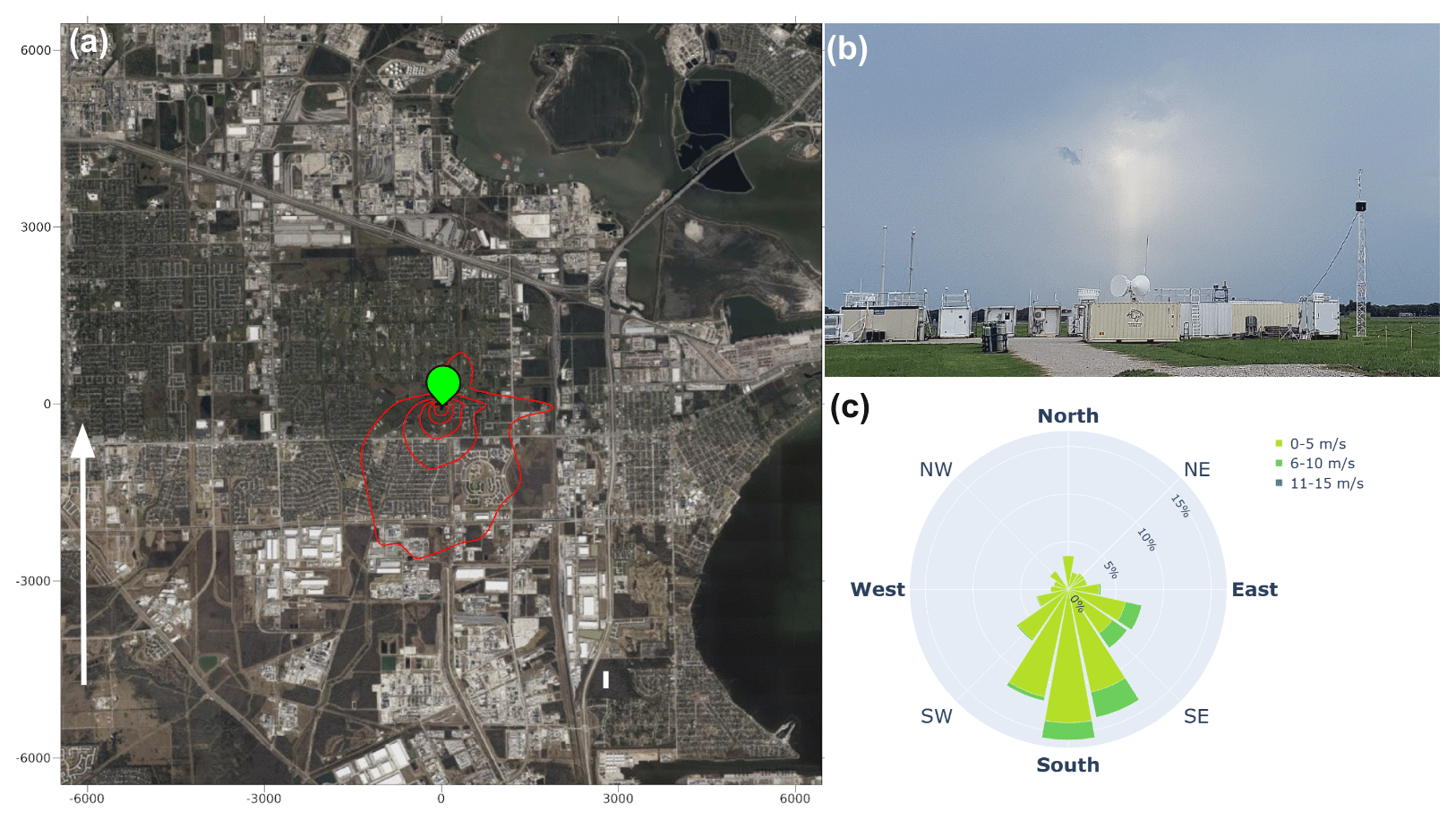
Figure 1 (a) The location of the AMF (green location marker) with a red polygon representing the flux footprint area. Map data: © Google, CNES/Airbus, Houston–Galveston area council, Landsat/Copernicus, Maxar Technologies, Texas General Land Office, US Geological Survey, USDA/FPAC/GEO, 2023. The white arrow gives the prevailing wind direction during the campaign. (b) Picture of the AMF setup. (c) Wind rose diagram for wind direction and speed during the sampling period.

2.2 Meteorology data

The Eddy Correlation Flux Measurement System (ECOR) provides measurements of the latent and sensible heat flux, as well as the friction velocity (Sullivan et al., 2021). The instrument uses a Windmaster 3D sonic anemometer (Gill Instrument, Saltmarsh Park, 67 Gosport Street, Lymington, Hampshire. SO41 9EG, United Kingdom) and infrared gas analyzer (LI 7500 and LI 7700) to measure high-frequency correlations between vertical velocity, air temperature, and water vapor density, resulting in vertical flux data at 30 min time resolution. The ECOR sensor height is ∼ 3 m. Latent and sensible heat flux values from the ECOR are used to calculate the saturation ratio flux (Supplement). The ARM Surface Meteorology Systems provided surface wind, pressure, temperature, relative humidity, visibility, and precipitation measurements at 1 min time resolution and at a sampling height of 8 m. For upper-air observation data, ARM provided interpolated sonde data containing relative humidity, specific humidity, temperature, horizontal wind, potential temperature, and dew point temperature on a fixed time–height grid. The data have 332 levels with a 1 min time resolution from the surface to a maximum of about 40 km. It is based on four launches per day.

2.3 Optical particle spectrometer

The AMF housed an optical particle counter (Grimm model 11-D, GRIMM Aerosol Technik GmbH & Co.KG, Dorfstraße 9, Ainring, 83404, Germany). The size distribution is binned into 31 equidistant channels ranging from 0.29 to 31.15 µm. Data are reported at 6 s of time resolution. The instrument includes a temperature and relative humidity sensor inside the optical block to monitor the thermodynamic state of the sample flow. The sample is dried to a relative humidity between 17 % and 40 % using a single-tube Nafion dryer: MD-700 by Perma Pure (1001 New Hampshire Ave, Lakewood, New Jersey 08701, USA).

2.4 Doppler lidar

2.4.1 Instrument

The DOE ARM program maintains a network of coherent Doppler lidar instruments, which are manufactured by Halo Photonics (Brockamin, Leigh, Worcestershire United Kingdom WR6 5LA GB). The Doppler lidar transmits at a wavelength of 1.548 µm, with ∼ 150 ns (22.5 m) pulse width and < 100 µJ pulse energy at a rate of 15 kHz, providing time- and range-resolved measurements of attenuated backscatter and radial velocity (Newsom and Krishnamurthy, 2020; Newsom et al., 2017). When operated in vertical fixed-point mode, the system measures vertical velocity at 1 Hz temporal and 30 m vertical spatial resolution. The lowest acceptable range gate is 105 m. The primary scattering mechanism is atmospheric aerosol. To date, the main application of this instrument has been the observation of turbulence within the boundary layer (Newsom et al., 2015; Williams and Qiu, 2023). When operated in hemispheric scanning mode, the instrument yields 2D wind fields as a function of height. The DOE ARM program collected the lidar data. The instruments are operated by DOE personnel, and data are distributed through publicly accessible archives (Newsom and Krishnamurthy, 2021; Shippert et al., 2022). Data in the archive have undergone a first pass of data processing. The vertical fixed-point data files, which are primarily used here, contain attenuated backscatter coefficients, signal-to-noise ratios, and vertical velocities at approximately 1 s intervals.

2.4.2 Relationship between particle size distribution and lidar backscatter

The lidar backscatter is attenuated by the two-way transmission through the atmosphere. The true backscatter can be found via (Platt and Collins, 2015)

$$\begin{array}{}\text{(1)}& \mathit{\beta }\left(r\right)={\displaystyle \frac{{\mathit{\beta }}_{\mathrm{att}}\left(r\right)}{\mathrm{1}-\mathrm{2}\mathrm{LR}{\int }_{r_{\mathrm{1}}}^{r_{\mathrm{2}}}{\mathit{\beta }}_{\mathrm{att}}\left(r\right)\mathrm{d}r}},\end{array}$$

where β(r) is the true backscatter coefficient, β_att(r) is the measured attenuated backscatter coefficient, LR is the lidar ratio defined in Eq. (2), and the integration is carried out between ranges r₁ and r₂. In Eq. (1) it is assumed that the lidar ratio does not vary with range. The true backscatter coefficient and attenuated backscatter coefficient are equal in the first range gate. The lidar ratio represents the ratio of the extinction cross-section and 180^∘ backscatter cross-section and varies between 5 and ∼ 100 sr. Its value depends on the wavelength, aerosol refractive index, aerosol size distribution, aerosol hygroscopicity, and the presence of absorbing gases in the atmosphere. Most prior studies have focused on systems with wavelengths 355, 532, and 1064 nm. Consequently, there is limited information about values for LR for wavelength > 1 µm. However, the lidar backscatter and lidar ratio can be estimated from the aerosol size distribution, aerosol hygroscopicity, and Mie theory.

$$\begin{array}{}\text{(2)}& {\displaystyle }{\mathit{\alpha }}_{\mathrm{mie}}={\int }_{\mathrm{0}}^{\mathrm{\infty }}{\displaystyle \frac{\mathit{\pi }{D}^{\mathrm{2}}}{\mathrm{4}}}{Q}_{\mathrm{ext}}\left(\mathit{\lambda },m,D\right){\displaystyle \frac{\mathrm{d}N}{\mathrm{d}\ln D}}\mathrm{d}\ln D\text{(3)}& {\displaystyle }{\mathit{\beta }}_{\mathrm{mie}}={\int }_{\mathrm{0}}^{\mathrm{\infty }}{\displaystyle \frac{\mathit{\pi }{D}^{\mathrm{2}}}{\mathrm{4}}}{Q}_{\mathrm{back}}\left(\mathit{\lambda },m,D\right){\displaystyle \frac{\mathrm{d}N}{\mathrm{d}\ln D}}\mathrm{d}\ln D\end{array}$$

Here, α_mie is the extinction coefficient derived from Mie theory, β_mie is the aerosol lidar backscatter coefficient derived from Mie theory, D is the particle diameter (m), Q_ext and Q_back are the extinction and backscatter efficiencies determined from Mie theory, d$N/\mathrm{d}$lnD is the aerosol size distribution in units of spectral density, λ is the wavelength (of the lidar), and $m=n+ki$ is the complex aerosol refractive index with a real (n) and imaginary (k) component. The integration is performed over the entire size distribution. The Mie solution assumes that the particles are spherical. The modeled lidar ratio is

$$\begin{array}{}\text{(4)}& \mathrm{LR}={\displaystyle \frac{{\mathit{\alpha }}_{\mathrm{mie}}}{{\mathit{\beta }}_{\mathrm{mie}}}}.\end{array}$$

The effects of scattering and extinction by molecules are not considered here.

At elevated relative humidity particles may swell and take up water. The refractive index of the mixed particle can be obtained from the volume-weighted average of the refractive indexes of the dry aerosol and water (Shettle and Fenn, 1979) and the water content estimated using the aerosol hygroscopicity parameter (Petters and Kreidenweis, 2007):

$$\begin{array}{}\text{(5)}& m=m_{\mathrm{w}}+\left(m_{\mathrm{aer}}-m_{\mathrm{w}}\right){\left(k{\displaystyle \frac{a_{\mathrm{w}}}{\mathrm{1}-a_{\mathrm{w}}}}+\mathrm{1}\right)}^{-\mathrm{1}},\end{array}$$

where m is the refractive index of the wet particle, m_w is the refractive index of pure water, m_aer is the refractive index of the dry aerosol particle, a_w= RH/100 % is water activity neglecting the Kelvin effect, and κ is the hygroscopicity parameter. The refractive indices $m=n+ki$ include a real (n) and imaginary (k) component. Equation (5) is derived by combining Eq. (6) in Shettle and Fenn (1979) and Eq. (1) in Carrico et al. (2010).

Figure 2 illustrates the change in optical properties with RH as modeled via Eqs. (1)–(5) and using the average size distribution measured by the OPC on 2 August 2022. A few notable trends can be summarized as follows. The backscatter coefficient β_mie varies $\sim \pm$50 % between 0 % and 80 % RH. However, most of the variability is within ±20 %. The function only weakly depends on the assumed hygroscopicity parameter. For real refractive indices n > 1.5, the backscatter coefficient can decrease with increasing RH. Increasing the RH increases this scattering cross-section due to hygroscopic growth. However, the backscatter decreases due to a decrease in the refractive index. For aerosols with a larger refractive index, the latter effect can dominate in the 40 %–90 % RH range. The modeled lidar ratio varies between ∼ 20 and 80 sr. Under dry conditions, the main controlling factor of the lidar ratio is the refractive index. Larger values of n amplify backscatter and thus result in a lower lidar ratio. Larger values of k amplify extinction and thus increase the lidar ratio. The lidar ratio can increase up to a factor of 2 with increasing RH, consistent with previous similar numerical simulations (Ackermann, 1998; Zhang et al., 2022).

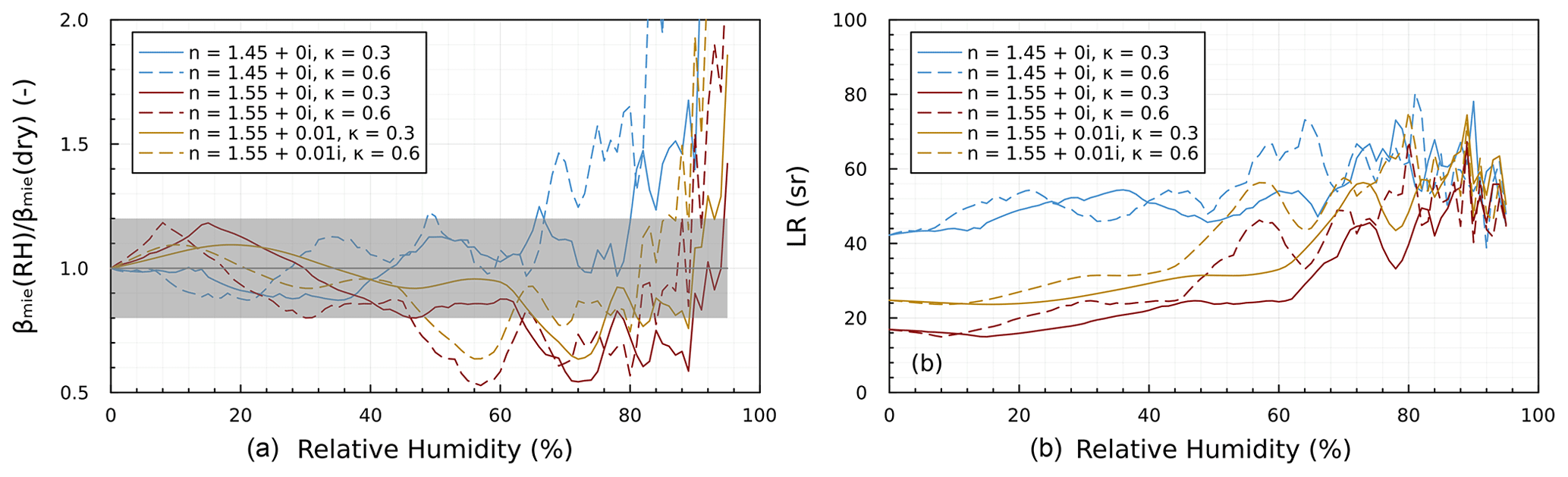
Figure 2 Change in aerosol optical properties with relative humidity as a function of refractive index and hygroscopicity. (a) Change in β_mie as a function of relative humidity. Color indicates the assumed refractive index. Solid and dashed lines correspond to κ= 0.3 and κ= 0.6, respectively. The gray shading indicates ±20 % variability. (b) Lidar ratios as a function of relative humidity.

The modeled β_mie is primarily sensitive to changes in aerosol number concentration and to a lesser extent the shape of the size distribution of particles in the 1 < D < 10 µm diameter range. Figure 3 shows a statistical analysis of the relationship between the aerosol size distribution and optical properties for 2 August 2022. The assumed refractive index is m= 1.55 + 0i. The value was picked arbitrarily due to a lack of knowledge of the refractive index of the aerosol and is used for illustration purposes. The aerosol size distribution shown in Fig. 3a (red fitted line) shows a coarse mode with a mode diameter ∼ 1 µm. Figure 3b shows that particles 2 < D < 6 µm contribute most of the signal to the total backscatter coefficient. Figure 3c shows the correlation of the integrated number concentration for particles D > 3 µm against the total β_mie. Linear regression of these data (R²= 0.98) can be used to relate an observed β to aerosol number concentration. The regression yields an intercept value that corresponds to the β_mie that is not explained by particles D > 3 µm. As indicated in Fig. 2a, the modeled β_mie depends weakly on RH. This implies a dependence of the regression slope on RH. Indeed, the example in Fig. 3d shows a slightly smaller slope for the assumed RH = 80 %. The regression analysis can be applied to arbitrary lower size cuts for the integrated number concentration. One would expect the strength of the correlation to decrease if smaller size particles were included. For example, the correlation for number concentration with D > 0.01 µm and total β_mie is likely small, since Aitken- and accumulation-mode particles insignificantly contribute to the backscatter. However, number concentrations within the coarse mode will be strongly autocorrelated if the shape of the coarse-mode distribution is unchanged. In this case, the numbers of D > 1 µm, D > 3 µm, and D > 7 µm will all yield a strong correlation with the total β_mie. Figure 3c tests the extent to which the correlation degrades for different lower size thresholds. This example shows R² > 0.75 even for a lower threshold D_lo= 0.53 µm but essentially no correlation for D_lo < 0.5 µm. The degradation of the correlation is evident as larger scatter in Fig. 3e and f compared to Fig. 3a. Although the details change due to day-to-day variability of the shape of the size distribution, the assumed refractive index, and the assumed hygroscopicity, the overall trends in Fig. 3b–f are repeatable. It is proposed that the empirical regressions shown in Fig. 3d–f, combined with a sensible D_lo, can be used to retrieve aerosol number concentration N(D > D_lo) from measured lidar backscatter coefficients.

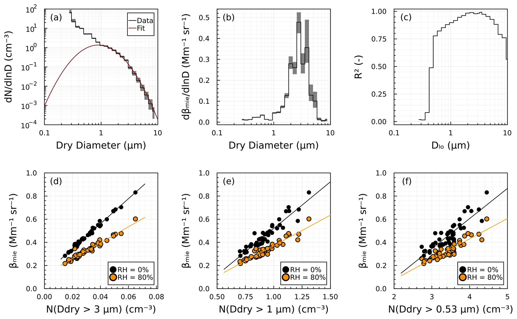
Figure 3 Statistical analysis of 1 d of aerosol size distributions. (a) Average aerosol size distribution measured by the OPC. The gray shading indicates the interquartile range. The red line shows a lognormal fit to the coarse mode. (b) Average size-resolved modeled β_mie, expressed as spectral density. The gray shading indicates the interquartile range. (c) Pearson correlation coefficient between N(D_dry > D_lo), the OPC integrated number of particles with diameter exceeding a lower threshold D_lo, and β_mie at RH = 0 %. (d) Correlation between integrated β_mie (all sizes) and measured number concentration > 3 µm. Each point corresponds to a 30 min time average. Solid lines indicate a linear fit. Colors indicate the assumed relative humidity. (e) Same as panel (d) but for number concentration > 1 µm. (f) Same as panel (d) but for number concentration > 0.53 µm.

Optical models like the one given by Eqs. (1)–(5) have been used successfully to relate OPC size distributions and backscatter for lidar returns from polar stratospheric clouds and cirrus clouds (Cairo et al., 2011; Snels et al., 2021). Here, however, the aerosol refractive index, the aerosol hygroscopicity, the contribution from molecular absorption to extinction, and the particle aspherical shape are unknown. Furthermore, the Doppler lidar backscatter is obtained via factory calibration (Newsom and Krishnamurthy, 2020). A back-of-the-envelope comparison of aerosol optical depth inferred from lidar backscatter against aerosol optical depth from the AErosol RObotic NETwork (AERONET) at a nearby site shows that the lidar backscatter correlates strongly with aerosol optical depth, but its value may be biased high. Combined, these uncertainties are too large to rely on the optical model alone to relate observed inverted backscatter to particle number concentration. Instead, this work relies on empirical correlations between the lidar-observed attenuated backscatter at z= 105 m (the lowest range gate) stratified by relative humidity and surface-based particle number concentration. Note that the two-way attenuation of the backscatter close to the ground is minimal and attenuated backscatter at z = 105 m approximately equals the true backscatter.

Figure 4 summarizes the campaign average correlation between the lidar-observed attenuated backscatter at z= 105 m and particle number concentrations D_lo > 0.53, D_lo > 1.03, and D_lo > 3.25 µm. The height z= 105 m is the lowest range gate to the surface that has complete time coverage above the signal-to-noise ratio. The shown correlations are analogous to those shown from the model in Fig. 3c. For the regression analysis, a lower threshold in number concentration was imposed (N > 2, 0.5, and 0.02 cm⁻³ for D_lo > 0.53, > 1.03, and D_lo > 3.25 µm, respectively). Below this threshold the correlations are poor, and the regression analysis obscured the intercept value. The correlations show the same pattern as the model. An intercept of the regression line for N= 0 cm⁻³ indicates the portion of the backscatter that is not explained by particles with D > D_lo. The change in the slope with RH is relatively small and shows a slight decrease in backscatter at 50 % < RH < 65 %, which is qualitatively comparable to the trends in Fig. 2a. The Pearson correlation coefficients are similar for the three shown cutoff sizes. Moving the lower size threshold to the lowest diameter measured by the OPC (D_lo > 0.28 µm) results in poor correlations (R² < 0.2) for all RHs. This consistency with the model simulations in Fig. 3d is satisfying. The R² values decrease with increasing RH. At RH > 90 %, the correlation is poor (0.2 < R² < 0.5). This suggests either increasing interference of other backscattering particles at higher RH or increasing uncertainty due to uncertainty in the RH value itself. Specifically, the comparisons between the interpolated sonde product and the ground-based meteorological station suggest that the precision of the interpolated sonde RH is not better than ±7 % in absolute RH units (supporting information). Furthermore, the R² values decrease with height, suggesting interference from backscatter attenuation and/or decorrelation of the aerosol at height z with those at the surface. In summary, the results in Fig. 4 suggest that backscatter fluctuations are indicative of particle number concentration if backscatter exceeds the value of the intercept, if a threshold D_lo > 0.53 µm is selected, and if RH < 90 %.

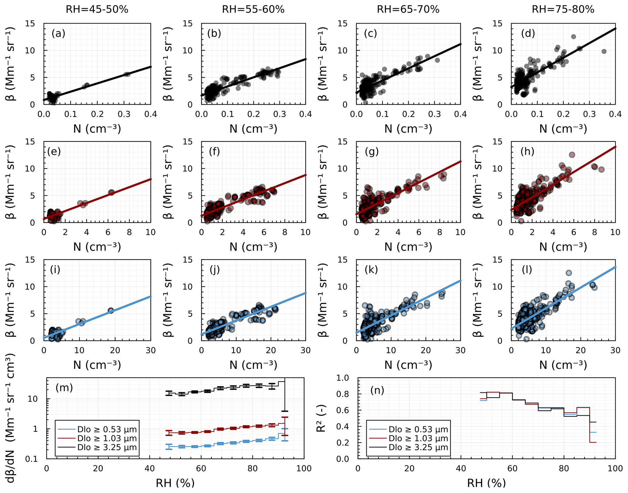
Figure 4 Panels (a–l): correlation of aerosol number concentration between the lidar-observed backscatter at z= 105 m and particle number concentrations D_lo > 3.25 µm (a–d), D_lo > 1.03 (e–h), and D_lo > 0.53 (i–l). The data are stratified by ambient relative humidity of 45 %–50 % (a, e, i), 55 %–60 % (b, f, j), 65 %–70 % (c, g, k), and 75 %–80 % (d, h, l). Panel (m) shows the slope of the regression line as a function of cutoff diameter D_lo and relative humidity using intervals [RH, RH + 5 %]. Panel (n) shows the Pearson correlation coefficient R² for the regression as a function of cutoff diameter D_lo and relative humidity using intervals [RH, RH + 5 %].

2.4.3 Derivation of backscatter flux

Backscatter flux is obtained using the eddy covariance technique,

$$\begin{array}{}\text{(6)}& F_{\mathit{\beta }}=<w^{\prime }{\mathit{\beta }}^{\prime }>,\end{array}$$

where w^′ and β^′ are the instantaneous fluctuations of vertical velocity and attenuated backscatter and < > indicates the time average. The measured backscatter coefficients are thresholded at a signal-to-noise ratio of −17 dB, which corresponds to a velocity precision of 20 cm s⁻¹ (Newsom and Krishnamurthy, 2020). The backscatter coefficient data show occasional spikes, possibly due to the transit of larger objects through the beam including birds. These spikes were removed using the following despiking algorithm. A low-pass filter with a cutoff frequency of 0.01 Hz and a fourth-order Butterworth filter function are applied to the backscatter coefficient. Values outside the 0.01 and 0.99 quantiles of the ratio of filtered and measured backscatter are considered spikes and replaced with the value from the filtered data, which approximately corresponds to the average ±100 s of the removed data point. This ensures continuity in the data during the spike event.

The Doppler lidar operates in fixed-point vertical orientation in contiguous blocks ∼ 780 s in length with vertical velocity and backscatter reported at ∼ 1 Hz frequency. This is followed by ∼ 120 s breaks while the instrument plan position indicator scans. The temporal spacing between consecutive timestamps is 1.025 ± 0.15 s. Here each contiguous block is used to derive a particle flux. First, the despiked backscatter data were detrended using a linear fit (Behrendt et al., 2020). Despiking removes spurious peaks from the data, while detrending subtracts both the mean and possible linear trends from the time series. Both are needed to compute accurate fluxes. Figure 5 shows an example of a contiguous block showing detrended and despiked vertical velocity and backscatter data. The corresponding signal variances are ${\mathit{\sigma }}_w^{\mathrm{2}}=$ 0.79 m² s⁻² and ${\mathit{\sigma }}_{\mathit{\beta }}^{\mathrm{2}}=$ 0.093 Mm⁻² sr⁻², respectively. The calculated backscatter flux is F_β= < $w^{\prime }{\mathit{\beta }}^{\prime }>=$ 1.6 × 10⁻⁵ s⁻¹ sr⁻¹.

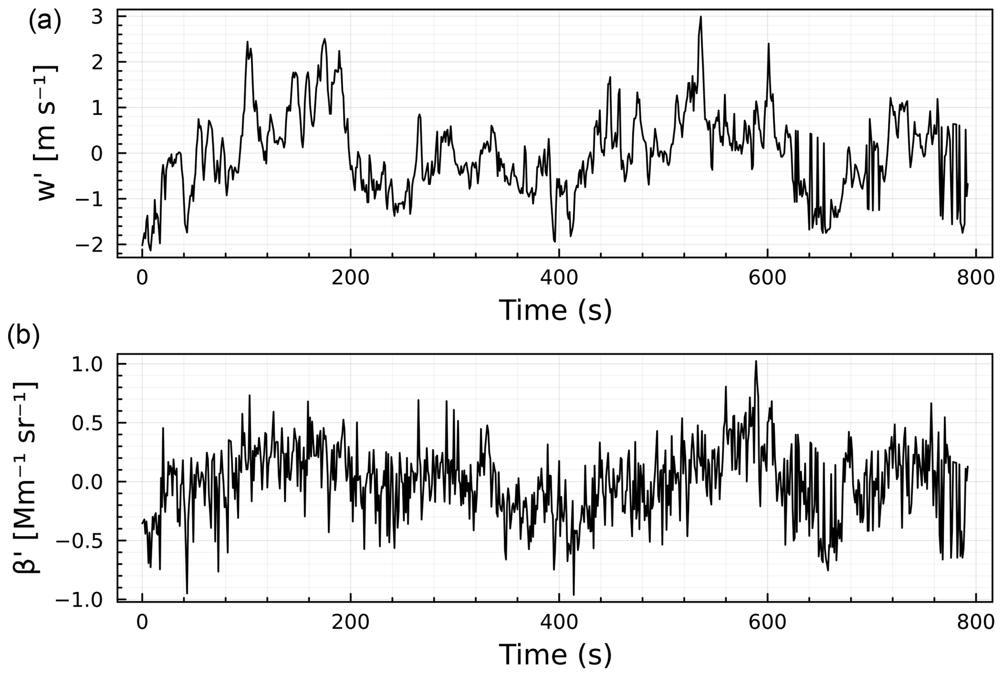
Figure 5 Example 780 s contiguous block of detrended and despiked (a) vertical velocity (w^′) and (b) backscatter data (β^′).

The lidar vertical velocity and backscatter data contain uncorrelated random noise stemming from a finite number of scatterers in the sampling volume and low photon counting statistics (Lenschow et al., 2000). The variance from uncorrelated noise can be separated from the signal using various methods. One common approach is the autocovariance method (Lenschow et al., 2000; Wulfmeyer et al., 2016). First, the autocovariance function A_x(τ) of the time series is computed via

$$\begin{array}{}\text{(7)}& A_x\left(\mathit{\tau }\right)=\mathrm{cov}\left(x_t,x_{t+\mathit{\tau }}\right),\end{array}$$

where x_t is the time series of interest, τ is the lag time, and cov is the covariance function. A_x(0) equals the variance of x_t. Next A_x(τ) from the data is fit to a model of the form

$$\begin{array}{}\text{(8)}& A_{\mathrm{model}}\left(\mathit{\tau }\right)=\mathit{\nu }-k{\mathit{\tau }}^{\left(\frac{\mathrm{2}}{\mathrm{3}}\right)},\end{array}$$

where ν and k are fitted parameters. The fit is obtained for lags up to the first zero crossing of A_x(τ). The model extrapolated to zero lag A_model(0) equals the noise-free variance. The variance attributed to noise is

$$\begin{array}{}\text{(9)}& {\mathit{\delta }}_x^{\mathrm{2}}=A_x\left(\mathrm{0}\right)-A_{\mathrm{model}}\left(\mathrm{0}\right).\end{array}$$

Finally, the integral timescale, I, is obtained from the fit parameters via

$$\begin{array}{}\text{(10)}& I={\displaystyle \frac{\mathrm{2}}{\mathrm{5}}}{\left({\displaystyle \frac{v}{k}}\right)}^{\frac{\mathrm{3}}{\mathrm{2}}}.\end{array}$$

Figure 6 shows an example of the autocovariance method applied to the contiguous data block shown in Fig. 5. The autocovariance (Eq. 7, black lines) is largest for lag zero and decreases for larger lag times. The model (Eq. 8, red lines) shows that the decrease with increasing lag is well-modeled using the $\mathrm{2}/\mathrm{3}$ power-law relationship. The derived noise variances, taken from the difference between the calculated covariance and model at lag time zero (Eq. 9), are δ²= 0.161 m² s⁻² and δ²= 0.052 Mm⁻² sr⁻² for vertical velocity and backscatter data, respectively. The integral timescales derived from Eq. (10) are I= 21 and I= 24 s, for vertical velocity and backscatter data, respectively. The contribution of the noise variance to the total variance, evaluated as ${\mathit{\delta }}^{\mathrm{2}}/{\mathit{\sigma }}^{\mathrm{2}}$ is ∼ 0.2 and ∼ 0.56 for the vertical velocity and backscatter data, respectively. This indicates that significant noise is present in the data. The derived integral timescales for the two series are similar. For lags > ∼ 50 s, the autocorrelation for both time series is minimal. The example in Fig. 6 illustrates how δ² and I were determined for each contiguous flux segment.

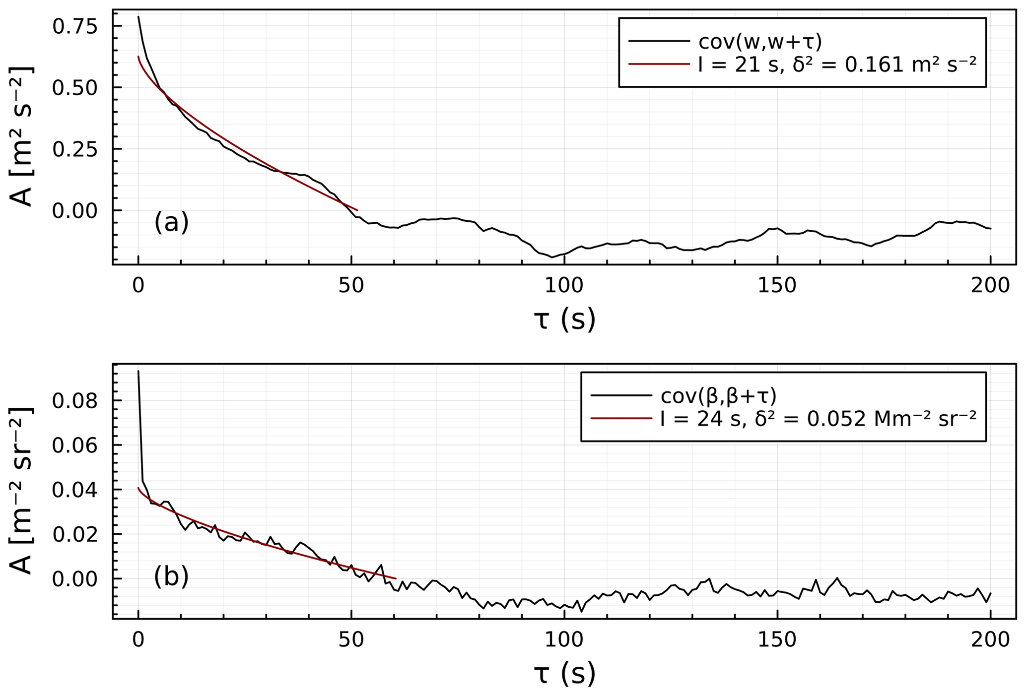
Figure 6 Autocovariance function for the data shown in Fig. 5. (a) Vertical velocity and (b) backscatter data. Black: A_x(τ), red: A_model(τ).

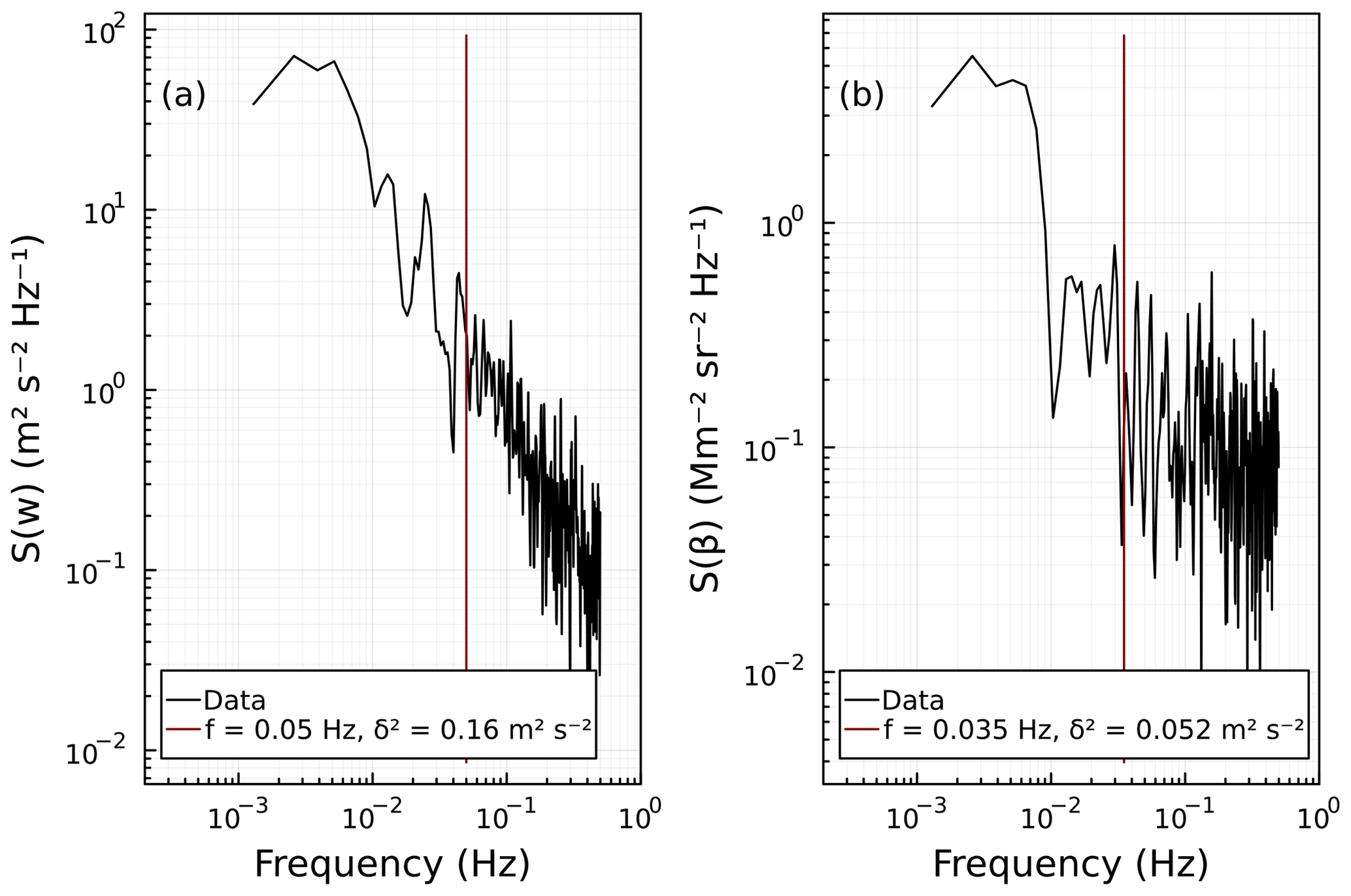
Figure 7 Spectral decomposition of the total variance for (a) vertical velocity and (b) backscatter for the contiguous data segment shown in Fig. 5. The integral ∫Sdf equals the total variance. The red line corresponds to the frequency cutoff such that the integral from the frequency cutoff to the Nyquist frequency corresponds to the noise variance δ² derived from the autocovariance analysis in Fig. 6.

Spectral analysis is used to estimate the frequency where noise overwhelms the signal. Figure 7 shows the spectral decomposition of the variance of vertical velocity S(w) and backscatter S(β) data. The spectra for S(β) are flat for frequencies larger than 0.035 Hz, which indicates white noise. Integrating ∫S(β)df from 0.035 Hz to the Nyquist frequency equals the noise variance ${\mathit{\delta }}_{\mathit{\beta }}^{\mathrm{2}}$ derived from the autocovariance analysis. Conversely, the spectra for S(w) do not flatten. Thus, the transition to white noise cannot be used to determine the noise limit. An estimate of the noise variance ${\mathit{\delta }}_w^{\mathrm{2}}$ can be found by integrating ∫S(w)df from 0.05 Hz to the Nyquist frequency. The visual depiction and the magnitude of these thresholds are similar for other contiguous segments. This suggests that derived backscatter fluxes for frequencies > ∼ 0.035 Hz are not well-resolved due to noise in the lidar signal.

2.4.4 Quality control and uncertainties

1. Random noise error. The random noise error in the flux F_β is approximated for each contiguous segment using Eq. (A22) in Wulfmeyer et al. (2016):

   $$\begin{array}{}\text{(11)}& {\mathit{\sigma }}_{\mathrm{noise}}\cong \sqrt{<{{\mathit{\beta }}^{\prime }}^{\mathrm{2}}>{\displaystyle \frac{{\mathit{\delta }}_w^{\mathrm{2}}}{N}}+<{w^{\prime }}^{\mathrm{2}}>{\displaystyle \frac{{\mathit{\delta }}_{\mathit{\beta }}^{\mathrm{2}}}{N}}},\end{array}$$

   where σ_noise is the uncertainty in the flux due to random noise, and ${\mathit{\delta }}_w^{\mathrm{2}}$ and ${\mathit{\delta }}_{\mathit{\beta }}^{\mathrm{2}}$ are noise variances derived from the autocovariance analysis.

2. Limit of detection (LOD). An alternative method to identify fluxes that are dominated by noise is the lag method (Spirig et al., 2005; Emerson et al., 2018; Islam et al., 2022). First, a lag is applied to the vertical velocity data. If the lag is sufficiently large, the computed $<w^{\prime }{\mathit{\beta }}^{\prime }>$ has contributions only from statistical noise. This can be taken as the limit of detection for the flux. The lag should be chosen to be sufficiently large to ensure that the autocovariance is zero, i.e., some multiple of the integral timescale. The median value of the integral timescale of the flux was ∼ 11 s and the 99th percentile is 63 s. We consider a lag of 200 s sufficient to evaluate the limit of detection using this method.

3. Sample statistics. The error associated with the limited number of eddies sampled within a flux segment can be estimated using Eq. (9) In Lareau (2020):

   $$\begin{array}{}\text{(12)}& {\mathit{\sigma }}_{\mathrm{sample}}=\mathrm{2}{\displaystyle \frac{I_{F\mathit{\beta }}}{T}}\left[F_{\mathit{\beta }}-\left({\mathit{\sigma }}_w^{\mathrm{2}}-{\mathit{\delta }}_w^{\mathrm{2}}\right)\left({\mathit{\sigma }}_{\mathit{\beta }}^{\mathrm{2}}-{\mathit{\delta }}_{\mathit{\beta }}^{\mathrm{2}}\right)\right],\end{array}$$

   where σ_sample is the uncertainty due to sample statistics, I_Fβ is the integral timescale of the flux, T is the sampling period (780 s), ${\mathit{\sigma }}_w^{\mathrm{2}}$ and ${\mathit{\sigma }}_{\mathit{\beta }}^{\mathrm{2}}$ are the total variances of vertical velocity and backscatter, respectively, and ${\mathit{\delta }}_w^{\mathrm{2}}$ and ${\mathit{\delta }}_{\mathit{\beta }}^{\mathrm{2}}$ are the noise variances of vertical velocity and backscatter, respectively. Note that the integral timescales of the individual parameters w and β are similar (mean I ∼ 22 and 26 s, respectively), but the integral timescale of the flux $<w^{\prime }{\mathit{\beta }}^{\prime }>$ is shorter (mean I ∼ 11 s).

4. Deviation from ensemble average. The flux error due to the departure of the observation from the domain-averaged flux is estimated via (Lareau, 2020; Lenschow et al., 1994)

   $$\begin{array}{}\text{(13)}& {\mathit{\sigma }}_{\mathrm{ensemble}}\cong \mathrm{2}{\displaystyle \frac{I_{F\mathit{\beta }}}{T}}{F}_{\mathit{\beta }}.\end{array}$$

5. Flux loss correction. Horst (1997) proposed correcting fluxes for sensors with a reduced frequency response by applying a cospectral transfer function to the ogive of the kinematic heat flux, computing the flux loss, and then correcting the observed flux for the missing contribution. This correction is built on the assumption that cospectra for fluxes of different scalar quantities are similar.

   $$\begin{array}{}\text{(14)}& F_{\mathrm{corr}}=F_{\mathit{\beta }}\left[\mathrm{1}+{\left(\mathrm{2}\mathit{\pi }{n}_{\mathrm{m}}{\displaystyle \frac{{\mathit{\tau }}_{\mathrm{c}}<u>}{z_{\mathrm{m}}}}\right)}^a\right]\end{array}$$

   Here, F_β is the measured flux, n_m= 0.085 and $\mathit{\alpha }=\mathrm{7}/\mathrm{8}$ are constants for neutral and unstable conditions, τ_c is the characteristic time constant of the sensor, $<u>$ is the mean wind speed at the sample height, and z_m is the measurement height. For stable stratification, α= 1 and n_m= 2 − 1.915$/$(1 + 0.5 $z/L$), where $z/L$ is the stability parameter, z is the measurement height, and L is the Obukhov stability length calculated from the surface ECOR data using the expression in Launiainen (1995). For unstable conditions $z/L$ < 0. Figure 7 and similar analyses for other flux segments suggest that the cutoff frequency for instrument noise is ∼ 0.035 Hz. The relationship between the 3 dB cutoff frequency and the $\mathrm{90}/\mathrm{10}$ response time of an instrument is estimated from the resistor–capacitor circuit analog of a low-pass filter. In that system the characteristic response time is given by a simple analytical solution ${\mathit{\tau }}_{\mathrm{c}}=\mathrm{0.35}/f$, where f is the 3 dB cutoff frequency (Andrews, 1999). Using 0.035 Hz as the cutoff frequency yields an estimate of τ_c ∼ 10 s. For unstable conditions, typical ratios for $F_{\mathrm{corr}}/F_{\mathit{\beta }}$ are ∼ 1.3–1.5.

6. Stationarity. A key assumption underlying the measurement of eddy correlation flux is stationarity. Strictly, stationarity implies that the temporal derivatives of the mean field approach zero during the flux detection period, i.e., d$w/\mathrm{d}t$ = 0, d$T/\mathrm{d}t$ = 0, and d$\mathit{\beta }/\mathrm{d}t=$ 0. Stationarity is rarely fully satisfied. Here we use the following metric to characterize stationarity (Foken and Wichura, 1996). The flux segment is divided into 5 min intervals. Then the relative difference between the flux of the entire segment and the mean of the fluxes from the 5 min flux legs is evaluated. Values less than 30 % are stationary. The stationarity metric, hereafter referred to as ξ, is reported alongside the $<w^{\prime }{\mathit{\beta }}^{\prime }>$ data.

7. Turbulence intensity. Reduced turbulence causing limited air mixing may result in a low bias of retrieved fluxes. At surface sites, the friction velocity u^* can be used to identify periods of limited air mixing (Papale et al., 2006; Barr et al., 2013). It is unclear if a u^* criterion can be applied to lidar data at z= 105. We therefore evaluated the turbulent kinetic energy (TKE) at z= 105 m from the colocated hemispheric scanning Doppler lidar. TKE can be used as a screening criterion to determine if the sample is inside the turbulent mixed layer (Vakkari et al., 2015). We use a criterion of TKE < 10⁻⁵ cm⁻² s⁻³ to flag periods wherein reduced turbulence may potentially have biassed the flux. The threshold was picked qualitatively as an indication of the presence of turbulence based on Fig. 4a in Vakkari et al. (2015). As will be discussed later, our conclusions are not sensitive to this threshold.

8. Precipitation. Precipitation may bias the measured Doppler velocity from lidar and can produce spurious backscatter returns (Aoki et al., 2016). Some of these may be removed by the despiking algorithm. Nevertheless, the flux data where any precipitation was measured during a flux segment were flagged and removed in subsequent data analysis.

9. Flux footprint. The flux footprint parameterization by Kljun et al. (2015) was used to calculate the footprint. An advantage of this model is that it can be used outside surface layer conditions and for non-Gaussian turbulence. Variations in lateral velocity and turbulence fluxes are considered. This parameterization is suitable for measurement heights > 20 m. Friction velocity used in this parameterization was obtained from the scanning Doppler lidar deployed at TRACER. Planetary boundary layer height was obtained from the North American Mesoscale Forecast System (NAM) model. Coniglio et al. (2013) compared different PBL schemes with radiosonde observations and came up with the conclusion that the NAM model produced the smallest mean absolute error. Hence the NAM model was used in this study. The surface temperature from the surface meteorological station at the site was used as the temperature at z= 105 m due to the lack of high-resolution temperature data at that height. However, the calculated flux footprints are not sensitive to the choice of temperature variable.

2.4.5 Example backscatter flux data

Figure 8 demonstrates the application of the various data quality control and uncertainties metrics. Figure 8a shows a 3 d time series of the noise-thresholded and despiked backscatter curtain for broader context. The backscatter shows values more than 100 Mm⁻¹ sr⁻¹ during nighttime (UTC) at z∼ 400 m (pink colors), likely due to the presence of low clouds. Since our analysis focuses on z= 105 only, no additional cloud screening was performed on the dataset. Backscatter signals up to 1500 m are retrieved at approximately noon local time. Figure 8b shows the derived backscatter flux with stable conditions identified via $z/L$ > 0 being grayed out. Superimposed in red is the limit of detection (LOD) derived for each contiguous segment using the lag analysis. The observed fluxes significantly exceed the values from the LOD analysis. Note that the LOD fluxes can be positive or negative. In contrast, the observed F_β values are all positive (indicating particle emission from the surface). Figure 8c shows that most flux values are from data that pass the stationarity test, i.e., abs(ξ) < 0.3. Figure 8d shows flux-loss-corrected hourly averaged flux values during unstable conditions only. The gray shading comprises the cumulative uncertainty of σ_noise, σ_sample , and σ_ensemble and remains small relative to the absolute value of the retrieved backscatter flux. Taking the combined data quality and uncertainty metrics into account, the data in Fig. 8 show that the backscatter fluxes are statistically significant.

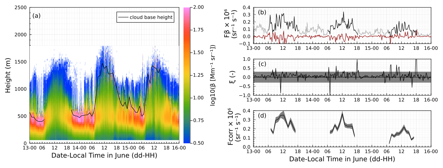
Figure 8 The 3 d time series starting 13 June 2022. (a) Time–height noise-thresholded attenuated backscatter curtain. Colors correspond to the log₁₀ of the backscatter value in units of Mm⁻¹ sr⁻¹. The solid black line shows the cloud-base height retrieved by the ceilometer. Periods with no cloud-base height data correspond to clear-sky conditions. (b) Black: backscatter flux at z= 105 m for each contiguous segment with $z/L<\mathrm{0}$ (unstable conditions), gray: backscatter flux at z= 105 m for each contiguous segment with $z/L<\mathrm{0}$ (stable conditions), red: limit of detection (LOD) computed using the lag method. (c) Stationarity metric ξ. The gray shading denotes the ±30 % threshold given by Foken and Wichura (1996). (d) Hourly averaged fluxes for unstable conditions after the application of the flux loss correction. The gray shading indicates the combined uncertainty derived from σ_noise $+{\mathit{\sigma }}_{\mathrm{sample}}+{\mathit{\sigma }}_{\mathrm{ensemble}}$.

2.4.6 Number flux from backscatter flux

Fluctuations in elastic backscatter correspond to fluctuations in aerosol number concentration (Pal et al., 2010). As demonstrated in Figs. 3 and 4, the Doppler lidar is sensitive to particle number concentration D > ∼ 0.5 µm. The relationship between backscatter and particle number is

$$\begin{array}{}\text{(15)}& \mathit{\beta }\left(S\right)={\left({\displaystyle \frac{\partial \mathit{\beta }}{\partial N}}\right)}_{\mathrm{S}}N\left(S\right)+c\left(S\right),\end{array}$$

where S is the saturation ratio (S= RH/100 %), β(S) is the backscatter at saturation ratio S, N(S) is the number concentration of particles larger than a specified threshold diameter, ($\partial \mathit{\beta }/\partial N{)}_{\mathrm{S}}$ is the slope, and c(S) is the intercept of the regression lines shown in Fig. 4a–l. In practice, ($\partial \mathit{\beta }/\partial N{)}_{\mathrm{S}}$ and c(S) were empirically evaluated in intervals [S; S + 0.05]. The ambient S value is obtained at the lidar height and sample time from the interpolated sonde product. The closest calibrated slopes and intercepts are used to derive N(S) from the observed β(S).

Figure 9 summarizes the retrieved particle number concentration from lidar backscatter via Eq. (15). Here retrievals are limited to conditions wherein RH < 90 %, there is no precipitation, and the observed backscatter exceeds 1.5 times the intercept value in Eq. (15). The latter limit is necessary to avoid retrievals where the backscatter is dominated by signals unrelated to particle number concentration. The cutoff value was selected to filter most noise while maintaining sufficient signal coverage. Increasing the value to > 1.5 does not further improve the accuracy of the comparison between the lidar and OPC shown in Fig. 9. The lidar-retrieved concentrations are visibly noisier, which is likely due to the noise in the backscatter data (Figs. 6 and 7) and the fact that the calibrated slopes were obtained from the campaign average, thus not accounting for variations in refractive index and hygroscopicity in the retrieval. Nevertheless, the retrieval captures the broad trends in particle number concentration, including the transition from lower-concentration to higher-concentration periods on 11 June, 15 July, and 20 July. Pearson correlation coefficients between the OPC and lidar-derived number concentrations are R²= 0.74 for the time series shown in Fig. 9c–e. The R² values are not identical but very similar, which is explained by the autocorrelation of number concentration within the coarse mode, i.e., because the shape of the coarse mode is approximately constant throughout the campaign. Overall, the results in Fig. 9 confirm that the variability in backscatter is related to changes in coarse-mode particle number concentration.

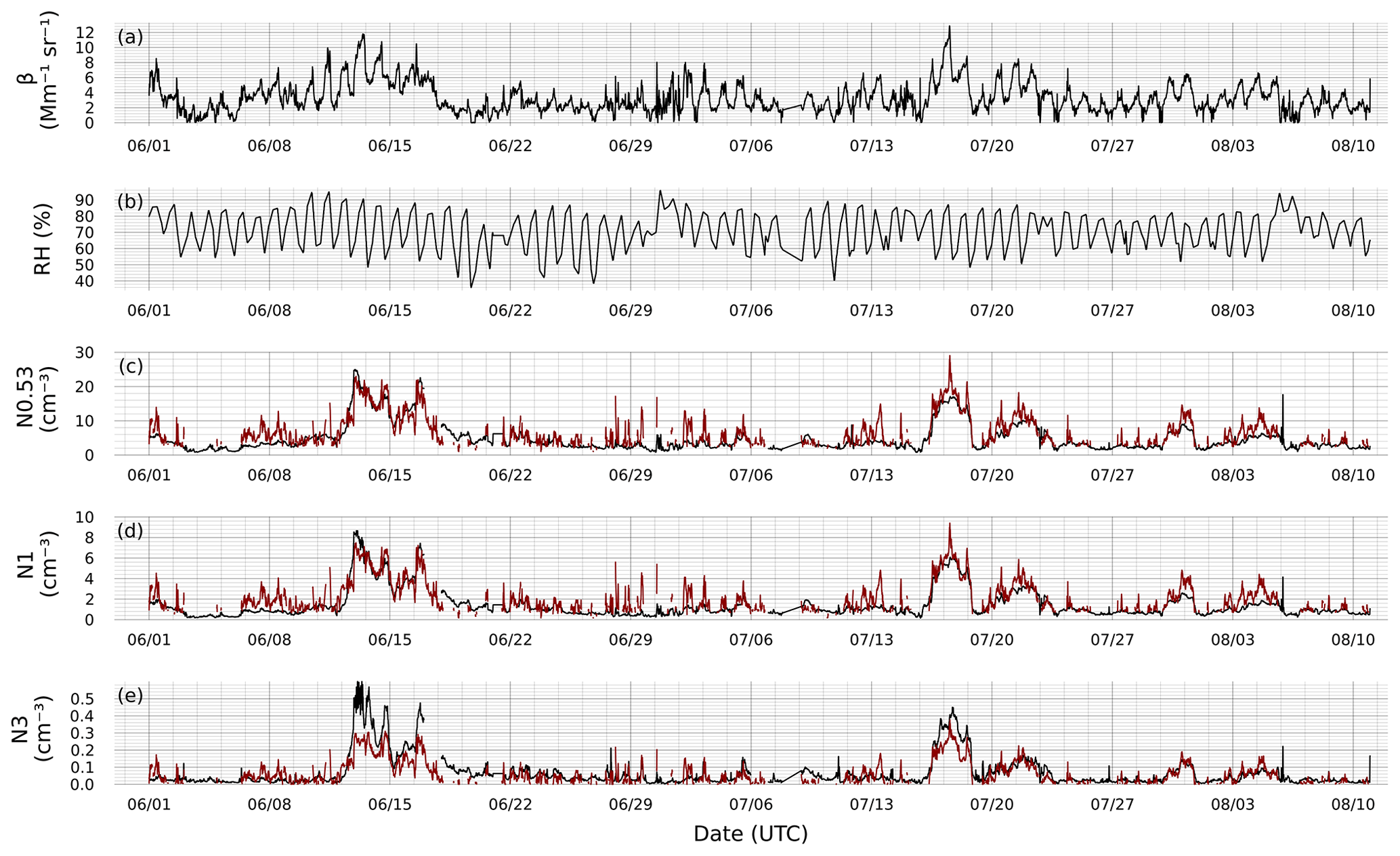
Figure 9 (a) Attenuated lidar backscatter at z= 105. (c) Relative humidity at z= 105 m from the interpolated sonde product. Data are presented at 30 min temporal resolution. (c) Particle number concentration for particles D > 0.53 µm measured at the surface by the OPC (black) and retrieved from the backscatter via Eq. (15). (d) Same as (c) for D > ∼ 1 µm size particles. (e) Same as (c) for D > ∼ 3 µm size particles.

Based on the preceding paragraph, we assert that high-frequency fluctuations in backscatter are related to high-frequency fluctuations in number concentration. To obtain the number flux from backscatter flux, high-frequency fluctuations in relative humidity also need to be considered (Fairall, 1984). This is because hygroscopic growth increases the particle size, which in turn affects the backscatter. During periods of intense sensible and latent heat flux, there are systematic differences in relative humidity or saturation ratio in updrafts and downdrafts, resulting in a saturation ratio flux. This saturation ratio flux can lead to an apparent particle flux that is not related to turbulent transport. Thus, turbulent flux measurements require correction for false fluxes during periods of high saturation ratio flux (Fairall, 1984; Kowalski, 2001; Vong et al., 2004; Islam et al., 2022).

To derive the influence of saturation ratio fluctuations on the lidar-derived number flux, we use an equation analogous to Eq. (18) in Fairall (1984):

$$\begin{array}{}\text{(16)}& {\mathit{\beta }}^{\prime }={\left({\displaystyle \frac{\partial \mathit{\beta }}{\partial N}}\right)}_{\mathrm{S}}{N}^{\prime }+{\left({\displaystyle \frac{\partial \mathit{\beta }}{\partial S}}\right)}_N{S}^{\prime }.\end{array}$$

Therefore, the number flux can be written as

$$\begin{array}{}\text{(17)}& \begin{array}{rl}<w^{\prime }{N}^{\prime }>& =<w^{\prime }{\mathit{\beta }}^{\prime }>/{\left({\displaystyle \frac{\partial \mathit{\beta }}{\partial N}}\right)}_{\mathrm{S}}-{\left({\displaystyle \frac{\partial \mathit{\beta }}{\partial S}}\right)}_N/\\ & {\left({\displaystyle \frac{\partial \mathit{\beta }}{\partial N}}\right)}_{\mathrm{S}}<w^{\prime }{S}^{\prime }>,\end{array}\end{array}$$

where $<w^{\prime }{N}^{\prime }>$ is the eddy covariance flux of particles and $<w^{\prime }{S}^{\prime }>$ is the saturation ratio flux. Evaluation of the terms ($\partial \mathit{\beta }/\partial S{)}_N$, ($\partial \mathit{\beta }/\partial N{)}_{\mathrm{S}}$, and $<w^{\prime }{S}^{\prime }>$ is provided in the Supplement. Note that the saturation ratio flux depends on the latent and sensible heat flux and can be either positive or negative. Furthermore, $<w^{\prime }{N}^{\prime }>$ is a net flux and includes contributions from surface emissions and dry deposition. The emission flux can be obtained by removing the estimated contribution from particle dry deposition (Nilsson et al., 2021):

$$\begin{array}{}\text{(18)}& F_{\mathrm{emission}}=<w^{\prime }{N}^{\prime }>+v_{\mathrm{d}}<N>,\end{array}$$

where v_d is the dry deposition velocity, and $<N>$ is the average number concentration. Note that by our convention positive $<w^{\prime }{N}^{\prime }>$ corresponds to an upward flux. In the absence of emissions (F_emission= 0), the observed $<w^{\prime }{N}^{\prime }>$ would be negative (downward), reflecting the dry deposition process and using the convention that the deposition velocity is a positive number. Deposition velocity is a function of particle diameter and land use type. Precise values remain poorly constrained within data showing approximately 2 orders of magnitude in scatter (Emerson et al., 2020). Here we consider v_d= 1 cm s⁻¹ as an approximate upper bound for particles in the 0.5 to 5 µm size range depositing on a grassland surface (Emerson et al., 2020).

Combining all the correction included in Eqs. (14), (17), and (18), the emission flux can be conceptually decomposed into four terms:

$$\begin{array}{}\text{(19)}& F_{\mathrm{emission}}=F+F_{\mathrm{flc}}+F_{\mathrm{wS}}+F_{\mathrm{dep}},\end{array}$$

where F= $<w^{\prime }{\mathit{\beta }}^{\prime }>/(\partial \mathit{\beta }/\partial N{)}_{\mathrm{S}}$ is the first-order conversion from backscatter to number flux and F_flc is the additional flux computed from the flux loss correction due to the low-frequency response of the Doppler lidar (Sect. 2.4). If no correction is required F_flc= 0. The sign of F_flc is the same sign as F. The term F_wS is the apparent contribution to the flux due to variation in the saturation ratio in updrafts and downdrafts. F_wS= −($\partial \mathit{\beta }/\partial S{)}_N/(\partial \mathit{\beta }/\partial N{)}_{\mathrm{S}}<w^{\prime }{S}^{\prime }>$ and can be either positive or negative. The term $F_{\mathrm{dep}}=v_{\mathrm{d}}<N>$ is always positive.

3 Results

Figure 10 shows a time series of the daily averaged lidar-retrieved emission flux for particles D > 0.53 µm. Only contiguous flux segments exceeding the limit of detection during unstable conditions are included. This excludes nighttime periods. Furthermore, flux legs with precipitation present and flux legs where turbulent kinetic energy was below 10⁻⁵ cm⁻² s⁻³ were excluded. Increasing the turbulent kinetic energy threshold filters more data but does not alter the overall trends shown in Fig. 10. Averaging over the entire day reduces the random errors from noise and short sampling periods (Fig. 8) and thus those errors are not further considered here. Several days show missing fluxes (white areas). These are predominantly from days on which all the < $w^{\prime }{\mathit{\beta }}^{\prime }>$ fluxes were below the limit of detection. All of the base flux values (F, black color), which are derived from the backscatter flux without further correction, are positive. This suggests that the site is dominated by emissions. Applying the flux loss correction (gold colors), which accounts for the reduced frequency response of the lidar, increases the base flux by ∼ 30 %–50 %. The correction for saturation ratio flux (F_wS) increases the flux further. The systematic increase is because on average $<w^{\prime }{S}^{\prime }>$ is negative during the daytime. However, the correction is small. The correction shown for dry deposition is based on an assumed v_d= 1 cm s⁻¹. In general, this correction is small relative to the reported emission flux values. However, the contribution may be appreciable during high-concentration periods. Nevertheless, the red band in Fig. 10 is likely an overestimate, as the true deposition velocity is likely an order of magnitude, or perhaps 2 orders of magnitude, lower than the assumed v_d= 1 cm s⁻¹ in Fig. 10 (Emerson et al., 2020).

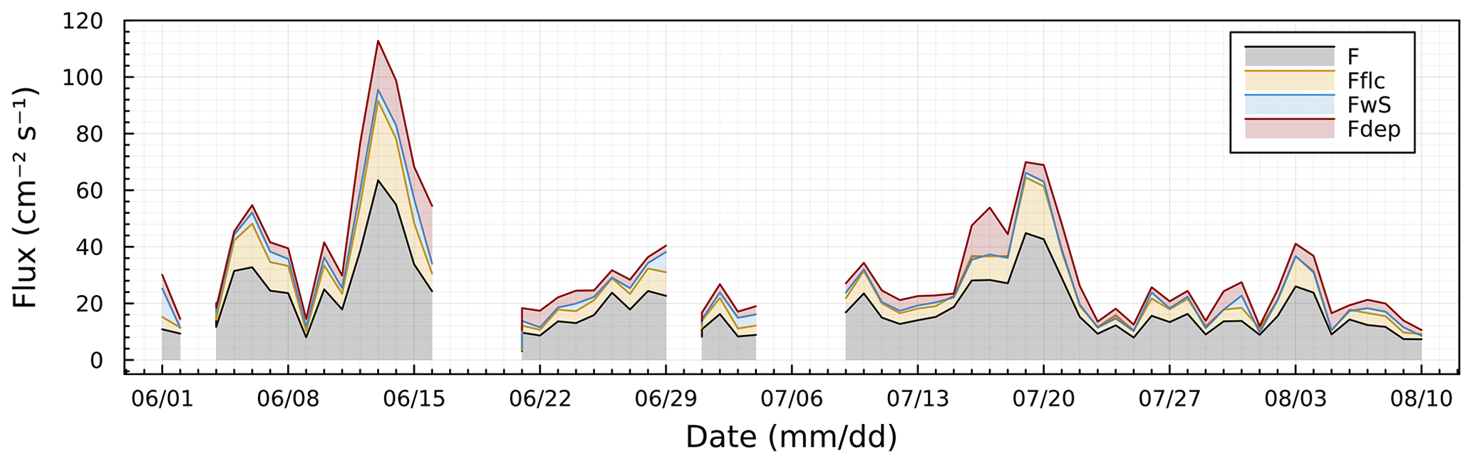
Figure 10 Temporal trend of daily averaged lidar-retrieved daytime emission flux for particles D > 0.53 µm. Colors correspond to the contributions to the emission flux as given in Eq. (19). Here F is the first-order conversion from backscatter to number flux, F_flc is the additional flux computed from the flux loss correction due to a low-frequency response of the Doppler lidar, F_wS is the apparent contribution to the flux due to variation in the saturation ratio in updrafts and downdrafts, and F_dep is the maximum estimated contribution of the deposition velocity to the flux. White areas correspond to dates on which fluxes were below the detection limit or insufficient data were available to compute flux corrections.

The emission fluxes in Fig. 10 range from ∼ 10 to ∼ 100 cm⁻² s⁻¹. For an assumed boundary layer height of 1 km and a day length of 100 000 s, a sustained flux of 10 cm⁻² s⁻¹ corresponds to an increase in number concentration of 10 cm⁻³ throughout the boundary layer due to the emission flux. Thus, the emission is significant relative to the background concentration, which varies between 1 and 20 cm⁻³ (Fig. 9c). Time series like Fig. 10 can be created for particle fluxes D > 1 and D > 3 µm. The temporal trend is identical to the data shown in Fig. 10 because they are scaled to the same backscatter flux. However, the magnitudes of the flux values are reduced to 33 % and 1.5 % of the emission flux for particles D > 0.53 µm, respectively. The flux footprint evaluated only for included flux segments (i.e., unstable conditions) is 3.1 ± 2.4 km (mean ±1 standard deviation) and includes a mix of grassland fields, asphalted surfaces, and urban housing developments. The footprint in Fig. 1 is an illustrative example of a simulated 2D footprint at the site. The time series show significant autocorrelation, with multi-day periods of higher fluxes, followed by multi-day periods of lower fluxes. This begs the following question. What are the sources of the emissions?

Possible candidate sources include dust emitted from the soil or biological particles emitted from vegetation. These sources would be expected to scale with meteorological conditions. For example, windblown soil dust would be expected to correlate with friction velocity (Kok et al., 2012). Biological emissions might be expected to respond to relative humidity (Wright et al., 2014; Yadav et al., 2022), with higher relative humidity triggering emission. Due to the sustained emission of coarse particles over long periods of time, it seems unlikely that anthropogenic point sources account for the emission. For example, hypothetical activities like traffic as well as airport landings and takeoffs would be expected to have a punctuated signal in the observed time series of particle flux. These would manifest in peaks with, for example, rush hour or weekday–weekend cycles. No such periodicity is apparent in the high-time-resolution flux data (not shown here). Natural sources, therefore, appear to be the most likely candidate.

Exploratory statistical analysis was performed by visually examining scatterplots between the observed daily averaged emission flux and potential explanatory variables, including wind speed, wind direction, friction velocity, surface temperature, surface relative humidity, latent heat flux, sensible heat flux, flux footprint, Monin–Obukhov length, and soil moisture (Supplement). Two candidate variables were identified from this statistical analysis to result in strong emissions: low surface relative humidity and high wind speed and friction velocity. Note that the fluxes are obtained during the daytime when the relative humidity is generally lowest due to surface heating. Further note that the Pearson correlation coefficient for a linear relationship between friction velocity and flux is poor. However, the relationship is fully consistent with that of a power law.

Figure 11 summarizes the dependency of the daily averaged emission flux on surface-derived friction velocity. In this analysis, only the first three terms on the right-hand side of Eq. (19) are included. Corrections for the deposition flux are not considered because the value is negligible for the expected typical value of v_d= 0.1 cm s⁻¹. The largest observed emission flux coincides with high friction velocity and low relative humidity. The emission flux scales approximately with u^*4, which is consistent with windblown dust emissions (e.g., Fig. 37 and discussion in Kok et al., 2012). Indeed, the emission flux can be parameterized as F= 3000 u^*4, where u^* is the friction velocity in m s⁻¹ and the emission flux F is in cm⁻² s⁻¹. It is important to note that the comparison to windblown desert dust is only an analogy, as the emission mechanisms are likely different from the saltation process occurring in sandy areas. We further note that no relationship was found between fluxes and soil moisture. Thus, the anticorrelation with relative humidity may or may not be coincidental. It is possible that days with sustained winds also had low relative humidity. However, it is also plausible that low relative humidity aided the lofting of the dust, especially from dust situated on asphalted and other urban surfaces. Longer-term studies will be needed to understand the emission mechanisms and important parameters that influence emissions.

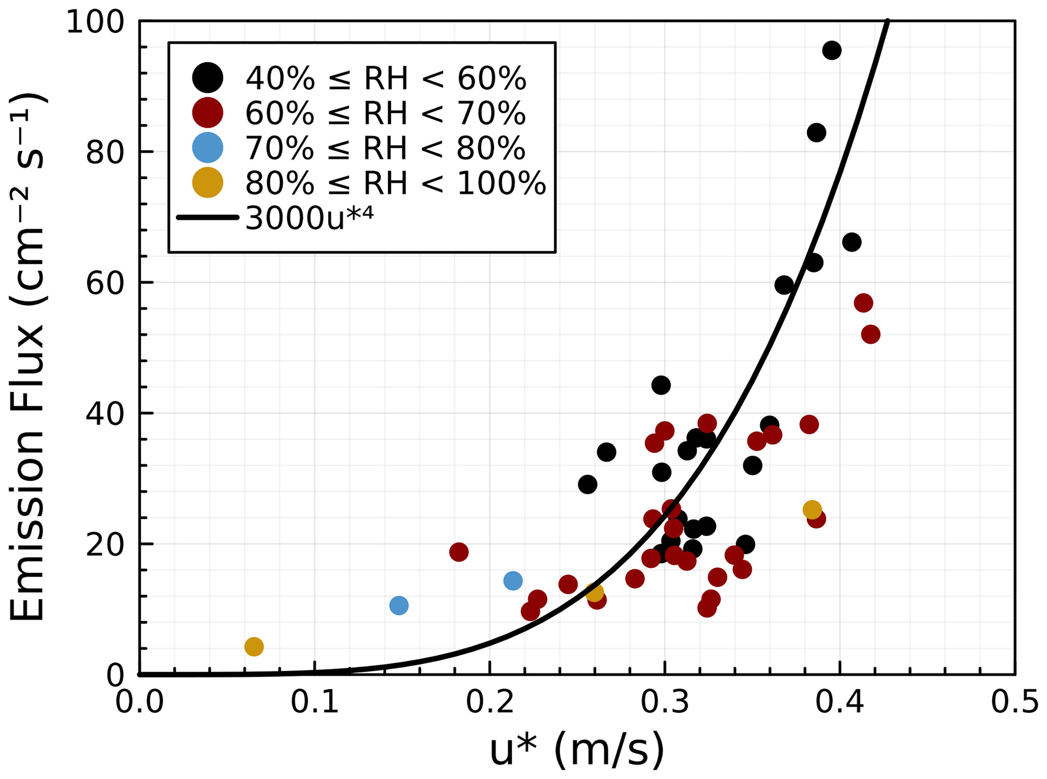
Figure 11 Variation of the daily averaged emission flux with surface-derived friction velocity. Colors show data stratification by relative humidity. The solid line illustrates an example of a power-law dependency of the emission flux.

4 Discussion and implications

This work has laid out a new methodology on how coherent Doppler lidar data can be used to obtain emission number fluxes. First, it was shown that Doppler lidar can be used to measure backscatter flux using the eddy covariance technique. Implementing the current state-of-the-science uncertainty analyses demonstrated that the backscatter fluxes are statistically significant (Fig. 8). Random errors due to signal noise were present but did not dominate the signal. Next, it was shown that lidar attenuated backscatter at z= 105 m can be related to particle number concentration above a size threshold using an empirical calibration between attenuated backscatter stratified by relative humidity and particle number concentration above a certain size threshold measured by an optical particle counter at the surface. Three thresholds were considered: D > 0.53, D > 1, and D > 3 µm. It was shown that this calibration led to a good correlation between particle number concentration inferred from lidar backscatter and particle number concentration observed at the surface (Fig. 9). This calibration was applied to derive the particle number emission fluxes from the backscatter flux, including flux loss correction for bias from a reduced frequency response by the lidar (Fig. 7 and Sect. 2, Horst 1997), correction for bias due to saturation ratio flux (Fairall, 1983), and correction for bias due to particle deposition (Nilssen et al., 2021). The magnitude of these corrections was shown to be appreciable but not dominant. The largest of these corrections was the flux loss correction due to a reduced frequency response, which led to ∼ 30 %–50 % reduction in the observed emission flux (Fig. 10). The temporal trend of the flux showed strong autocorrelation with multi-day periods of higher followed by multi-day periods of lower emission fluxes. The emission flux was correlated with wind speed and friction velocity and anticorrelated with surface relative humidity (Fig. 11). This suggests that the emissions are due to mechanical erosion from urban surfaces.

We are not aware of other coarse-mode particle flux measurements in urban environments. To place these emission data in context, we compare the emission flux reported here to other field measurements of emission fluxes from eroding soils (see Fig. 37 in Kok et al., 2012). Those measurements report mass fluxes varying between 10 and 100 000 µg m⁻² s⁻¹. The approximate mass for a 1 µm particle (roughly the mass-mode diameter of the coarse-mode distribution) is ∼ 10⁻⁶ µg. Applying this factor to the emission number flux in Fig. 11 yields emission fluxes between 0.1 and 1 µg m⁻² s⁻¹, which is much lower than the range of dust fluxes (Kok et al., 2012). The composition of the coarse mode in urban environments shows contributions from road dust, tire debris, and biological particles (Wu and Boor, 2021). We would expect the reported emissions to emanate from dust located on asphalted surfaces and exposed soil from grasslands and gardens.

Significant data quality screening and averaging were applied to the dataset here. This led to the exclusion of flux data under stable conditions (Monin–Obukhov length > 0) and in the presence of precipitation. These data are not necessarily bad. However, evaluating data under stable conditions, which predominantly occurred during nighttime and also coincided with low u^* and TKE conditions, will require more in-depth analysis to understand the importance and accuracy of the flux loss correction and footprint expansion that occurs in that regime. Furthermore, we mostly considered daily average fluxes. Higher-time-resolution data are available (e.g., Fig. 8d). These data are noisier (high variability from flux leg to flux leg) and generally show a diurnal trend with peak fluxes occurring near local noon. Understanding and fully quantifying these higher-time-resolution emission patterns may be important for understanding the influence of the emissions on cloud formation. The retrievals in this work were limited to a single vertical level at z= 105 m. In principle, this method will be suitable to also retrieve flux profiles, i.e., the variation of particle number flux with height. This work did not further pursue this for several reasons. First, the calibration of the signal against the surface optical particle counter (Fig. 4) becomes less certain when applied to backscatter at higher altitudes. This is due to increasing uncertainty due to elevated relative humidity (Fig. S1), the potential decoupling of higher layers from surface observations, and the loss of signal due to the two-way attenuation of the backscatter signal. Those issues can be overcome, at least in principle, by incorporating vertical profile measurements of particle concentration and by applying appropriate inversion to convert attenuated backscatter to backscatter. Second, measurements at higher altitudes will require careful screening for cloud events, boundary layer height, and boundary layer evolution. This is illustrated in Fig. 8a, which shows how clouds and a low signal-to-noise ratio would complicate automated evaluation of a time series at z= 1000 m. In summary, evaluation of vertical profiles may be possible in future studies but will require additional data and a case-by-case analysis approach. In aggregate, the applied methodology resulted in a first-pass analysis of the data. Some of the assumptions may be relaxed with additional analyses, resulting in additional information that may be derived from this and similar datasets.

Overall, the results here are promising to obtain emission fluxes using remote sensing techniques. One advantage of this approach is that the technique is relatively low-maintenance, thus allowing long-term measurements. The fluxes are obtained at 100 m or higher. Therefore, a high-frequency response instrument sampling at 10 Hz is not as critical because turbulent eddies are more coherent at higher altitudes. Another advantage is that the flux footprint increases with height, thus allowing the sampling of emissions from an area of several square kilometers. However, the lidar-derived number fluxes also have several limitations. The lidar backscatter is a convolution integral property, e.g., Eq. (3), that is sensitive to relative humidity. The relationship between backscatter and number flux will always be subject to the limitation of the assumptions made in the analysis. For example, a campaign-averaged calibration was used to relate backscatter to particle number, which neglects potential variations in the shape of the coarse-mode size distribution, variations in aerosol refractive index, variations in particle shape, and variations in aerosol hygroscopicity. The seriousness of these assumptions is difficult to evaluate because a large enough dataset is required to build the calibration in Fig. 4. Future studies may consider a longer-term dataset, subdivide the calibration into multiple time periods, and then evaluate the influence of using different calibrations on the retrieved number flux. Another limitation is the inherent noisiness of lidar backscatter data due to instrument noise and limited photon backscatter from the control volume. This might limit the application of this technique to regions where sufficient backscatter is available, as defined by a high signal-to-noise ratio. The overall limit of detection appears to exceed values of expected dry deposition fluxes in the sampled size range. For example, the largest estimate for the deposition flux is ∼ 10 cm⁻² s⁻¹ (Fig. 10). More realistic values of the dry deposition velocity would result in deposition fluxes of 1 or 0.1 cm⁻² s⁻¹. These values are unlikely to be resolvable with the Doppler lidar in this configuration and environment. Despite these limitations, the technique may have broad applicability to evaluate surface emissions from deserts, oceans, urban landscapes, and biologically active ecosystems, which all may release appreciable coarse-mode particles through wind- and weather-driven processes.