Unveiling the optimal regression model for source apportionment of the oxidative potential of PM₁₀

The capacity of particulate matter (PM) to generate reactive oxygen species (ROS) in vivo leading to oxidative stress is thought to be a main pathway in the health effects of PM inhalation. Exogenous ROS from PM can be assessed by acellular oxidative potential (OP) measurements as a proxy of the induction of oxidative stress in the lungs. Here, we investigate the importance of OP apportionment methods for OP distribution by PM₁₀ sources in different types of environments. PM₁₀ sources derived from receptor models (e.g., EPA positive matrix factorization (EPA PMF)) are coupled with regression models expressing the associations between PM₁₀ sources and PM₁₀ OP measured by ascorbic acid (OP_AA) and dithiothreitol assay (OP_DTT). These relationships are compared for eight regression techniques: ordinary least squares, weighted least squares, positive least squares, Ridge, Lasso, generalized linear model, random forest, and multilayer perceptron. The models are evaluated on 1 year of PM₁₀ samples and chemical analyses at each of six sites of different typologies in France to assess the possible impact of PM source variability on PM₁₀ OP apportionment. PM₁₀ source-specific OP_DTT and OP_AA and out-of-sample apportionment accuracy vary substantially by model, highlighting the importance of model selection according to the datasets. Recommendations for the selection of the most accurate model are provided, encompassing considerations such as multicollinearity and homoscedasticity.

1 Introduction

Ambient particulate matter (PM) is one of the key contributors to atmospheric pollution and is responsible for approximately 7 million premature deaths worldwide yearly (WHO, 2021). Many epidemiological studies have linked PM exposure to adverse health effects including (i) acute effects studies using time series and related studies to evaluate the immediate impact of PM exposure (Bell et al., 2004; Dominici, 2004; Pope and Dockery, 2006; Peng et al., 2009) and (ii) cohort studies aiming to evaluate the long-term effects of chronic PM exposure (Pelucchi et al., 2009; Crouse et al., 2012, 2015; Beelen et al., 2014; Ayres et al., 2008; Yu et al., 2021). These studies mainly focused on the association with PM mass concentrations. However, various research shows that the impacts of PM also depend on other factors such as chemical composition, size distribution, particle morphology, and biological mechanisms (Brook et al., 2010) . The capacity of PM to generate reactive oxygen species (ROS) in vivo has recently been introduced as a pivotal indicator of PM biological mechanism with direct implications for oxidative stress and cellular damage (Li et al., 2008; Lodovici and Bigagli, 2011; Mudway et al., 2020; Nelin et al., 2012; Rao et al., 2018; Ayres et al., 2008; Akhtar et al., 2010; Leni et al., 2020). The quantification of the PM capacity to oxidize biological media is called “oxidative potential” (OP) (Bates et al., 2019; Daellenbach et al., 2020; Dominutti et al., 2023). Various acellular assays of OP have been introduced, differentiating ROS generation mechanisms of PM (Dominutti et al., 2023; Calas et al., 2018). Dithiothreitol (DTT) and ascorbic acid (AA) assays are two of the commonly used procedures in the literature (Liu and Ng, 2023).

The relationship between PM chemical components and OP activities may indicate which components are the most prone to generating ROS (Calas et al., 2019; Godri et al., 2011; Yang et al., 2014; Janssen et al., 2014; Crobeddu et al., 2017; Szigeti et al., 2015, 2016; Calas et al., 2018). However, this research pathway struggles with the co-variation between measured and unmeasured PM components (Calas et al., 2018; Weber et al., 2018). An alternative approach is to examine the association between OP and sources of PM obtained using receptor models such as chemical mass balance, positive matrix factorization (PMF), or principal component analysis. PMF is the most popular method for its ability to quantify PM source contributions without extensive prior information on specific sources at the site studied (Belis et al., 2013; Viana et al., 2008; Paatero and Tappert, 1994; Brown et al., 2015; Paatero and Hopke, 2009).

Regression analysis is the most common and effective way to estimate the redox activity of receptor-model-derived PM sources (Bates et al., 2015; Deng et al., 2022; Li et al., 2023; Liu et al., 2018; Shangguan et al., 2022; Verma et al., 2014; J. Wang et al., 2020; Yu et al., 2019). Generally, this is achieved by regression analyses to characterize the relationship between OP activities (nmol min⁻¹ m⁻³) and PM source contributions (µg m⁻³). This approach provides the OP activities attributed to each microgram of each source (nmol min⁻¹ µg⁻¹), denoted as “intrinsic OP”, which can be used to calculate the contribution of each source for each observation day. Numerous regression models can be used for such OP source apportionment (SA), with multiple linear regression fitted by ordinary least squares (OLS) being the most common regression technique (Bates et al., 2015; Deng et al., 2022; Li et al., 2023; Liu et al., 2018; Shangguan et al., 2022; Verma et al., 2014; Y. Wang et al., 2020; Yu et al., 2019). Further, some studies exclude sources with negative intrinsic OP, assuming that negative OP activities are geochemically nonsensical (Bates et al., 2018; Weber et al., 2018). Additionally, weighted least squares can be used to introduce a weighting term, generally using the OP analysis uncertainties to take into account the measurement uncertainties of the OP assays (Borlaza et al., 2021; Daellenbach et al., 2020; Dominutti et al., 2023; Fadel et al., 2023; in't Veld et al., 2023; Weber et al., 2021). Finally, non-linear models, such as multilayer perceptron, have been used to try to capture possible non-linearities between OP activities and PM sources (Borlaza et al., 2021; Elangasinghe et al., 2014; D. Wang et al., 2023). However, no study to date has compared the performance and applicability of these various regression models. Each model entails different assumptions which should be carefully considered when selecting a given model.

This study aims to evaluate the variability in PM₁₀ OP SA techniques by comparing eight regression techniques: multiple linear regression fitted by OLS, weighted least squares (WLS), positive least squares (PLS), ridge regression (Ridge), least absolute shrinkage and selection operator (Lasso), generalized linear model (GLM), random forest (RF), and multilayer perceptron (MLP). These techniques are applied to apportion PM₁₀ OP_AA and PM₁₀ OP_DTT to PM₁₀ sources at six sites in France. The PM₁₀ SA outputs have been published by Weber et al. (2021), using a harmonized PMF methodology based on 1 year of sampling with similar chemical analyses for a large set of chemical tracers. The results of the PM₁₀ OP SA models are compared with regard to the estimated intrinsic PM₁₀ OP of each source, the out-of-sample accuracy of the apportionment, and the assumptions inherent in each model. The most appropriate model at each site is compared with OLS to quantify the difference between choosing a model based on data characteristics vs. using the most common approach. Finally, this study provides guidelines for selecting the most suitable model in the strategy for OP contribution regarding sources of PM₁₀. This holds particular significance in the context of the implementation of OP monitoring as a novel air quality metric as foreseen in research programs (such as RI-Urbans) and in the process of the revision of European Directive 2008/50/CE.

2 Methodology

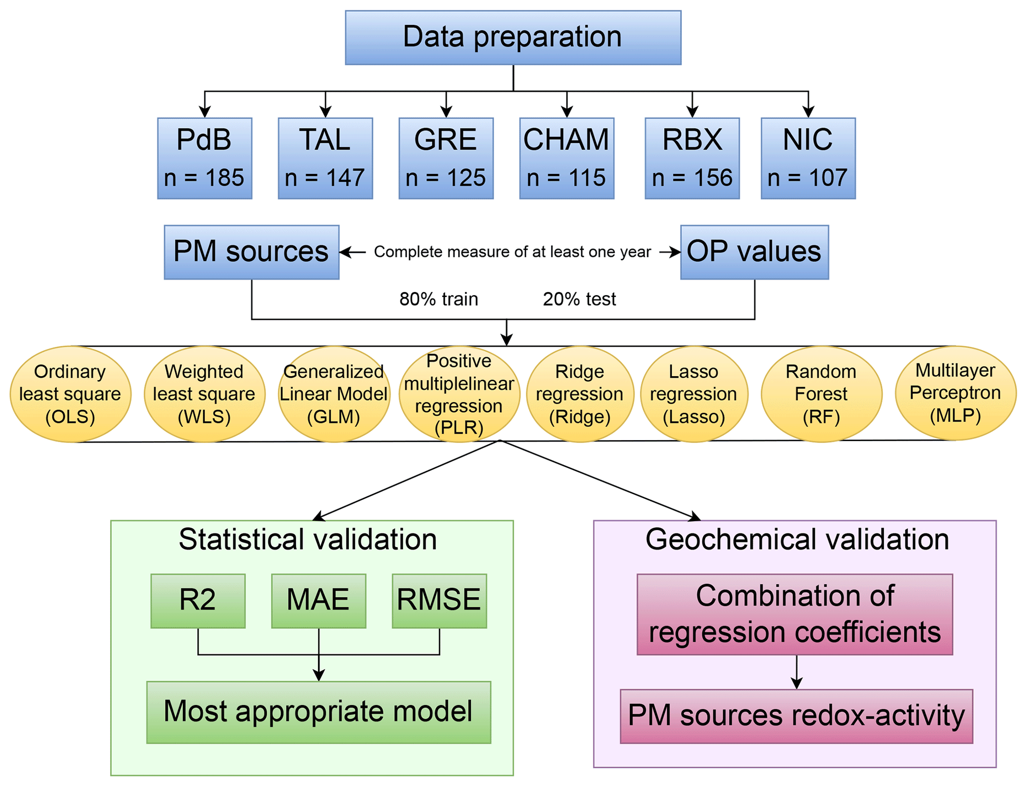
2.1 General organization of the study

Figure 1 illustrates the general workflow of this study. Sections 2.2, 2.3, and 2.4 describe the methods used to analyze the temporal evolution of PM₁₀ sources and PM₁₀ OP, identify collinearity among PM₁₀ sources, and examine homoscedasticity in the relationship between PM₁₀ OP and PM₁₀ sources. Section 2.5 describes the eight regression techniques (OLS, WLS, PLS, Ridge, Lasso, GLM, RF, and MLP), used for PM₁₀ OP SA. Each technique is applied to each site separately using PM₁₀ OP_v (nmol min⁻¹ m⁻³) as the dependent variable and PM₁₀ sources (µg m⁻³) as independent variables. The coefficient of the regression, called the “intrinsic PM₁₀ OP” of the source (nmol min⁻¹ µg⁻¹), represents the capacity of each µg of PM₁₀ from the given source to generate oxidative stress; the higher the intrinsic PM₁₀ OP of a source, the more redox-active. Each model is trained on a randomly selected (without replacement) 80 % subsample of the dataset and validated on the remaining 20 %. This process is repeated 500 times to estimate uncertainty, a method particularly needed for sources with strong seasonality. For WLS, PLS, Ridge, and Lasso models, PM₁₀ OP analytical errors were used as a weighting, implying that the PM₁₀ OP with the high analysis uncertainties has less influence on the model. These eight regression techniques were applied to find the relationship between PM₁₀ OP and PM₁₀ sources; however, PLS, Ridge, and Lasso were performed twice, with and without weighting, and consequently there are 11 results of regression techniques that will be presented. Section 2.6 describes the statistical validation of the models using root mean square error (RMSE), mean absolute error (MAE), and R-squared (R²). The geochemical validation is based on the regression coefficient (the intrinsic PM₁₀ OP) of each source. These are calculated separately for the training and testing data and averaged across the 500 sampling iterations.

Figure 1 Workflow comparison of the methodology for PM₁₀ OP source apportionment.

2.2 Study sites and PM₁₀ sources

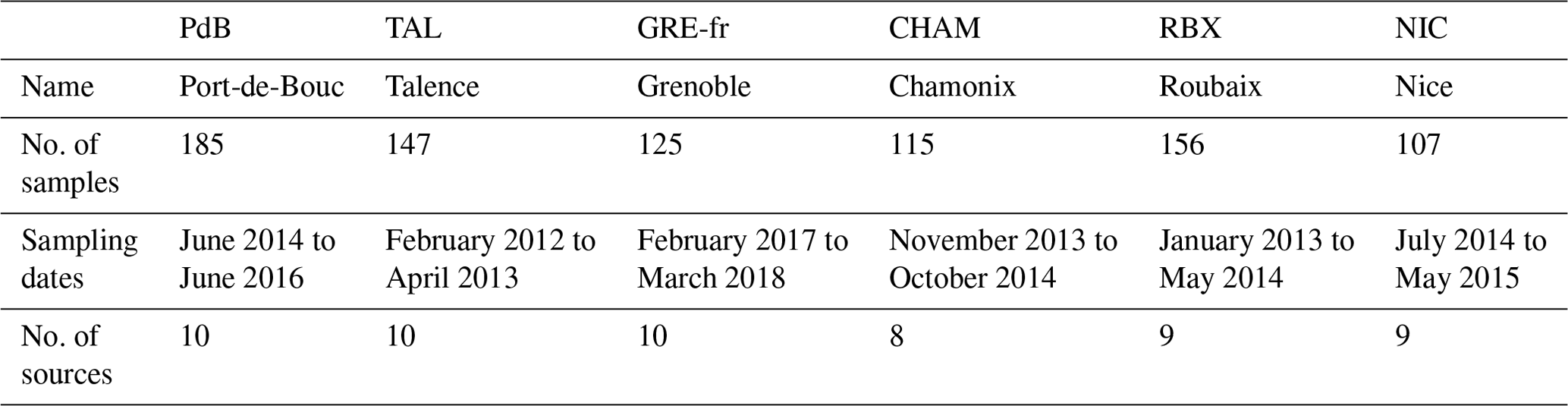
Six French sites are selected in this work for their different typologies: Roubaix and Nice (traffic sites within urban areas), Port-de-Bouc (industrial hotspot), Talence (urban background site), Grenoble and Chamonix (urban background sites in an alpine valley). At each site, sampling was conducted over at least 1 year to capture the complete annual evolution of PM₁₀ and its components. These sites and sampling series have been used and described by Weber et al. (2019).

In brief, daily filter samples were collected on pre-heated Pallflex quartz fiber filters every third day through high-volume sampling (DA80, Digitel). These filters were analyzed to determine the PM chemical species and OP activities. Further details regarding the chemical species and PM₁₀ OP analysis methodology can be found in Weber et al. (2019, 2021). Briefly, elemental carbon (EC) and organic carbon (OC) were analyzed using the EUSAAR2 thermo-optical protocol with a Sunset Laboratory analyzer. Major ionic components (Cl⁻, NO${}_{\mathrm{3}}^{-}$, SO${}_{\mathrm{4}}^{\mathrm{2}-}$, NH${}_{\mathrm{4}}^{+}$, Na⁺, K⁺, Mg²⁺, Ca²⁺) and methanesulfonic acid (MSA) were measured by ion chromatography (IC). Anhydro sugars and saccharides (including levoglucosan, mannosan, arabitol, sorbitol, and mannitol) were analyzed by high-performance liquid chromatography with pulsed amperometric detection (HPLC-PAD). Major and trace elements (Al, Ca, Fe, K, As, Ba, Cd, Co, Cu, La, Mn, Mo, Ni, Pb, Rb, Sb, Sr, V, and Zn) were determined by inductively coupled plasma atomic emission spectroscopy or mass spectrometry (ICP-AES or ICP-MS). Furthermore, colocated PM₁₀ measurements were conducted automatically at each site using the Tapered Element Oscillating Microbalance equipped with a Filter Dynamics Measurement System (TEOM-FDMS).

We used the PM₁₀ sources identified by Weber et al. (2019), who performed a separate PMF for each site using a harmonized approach for all sites (the same chemical species and measurement methods, the same procedure to estimate uncertainties, and the same constraints on the preliminary solutions). Table 1 provides a data description, including the sampling duration, the number of samples collected, and the PM₁₀ sources identified at each site, while Fig. 2 presents the location of the sites in France together with the respective proportion of each PM₁₀ source at each site.

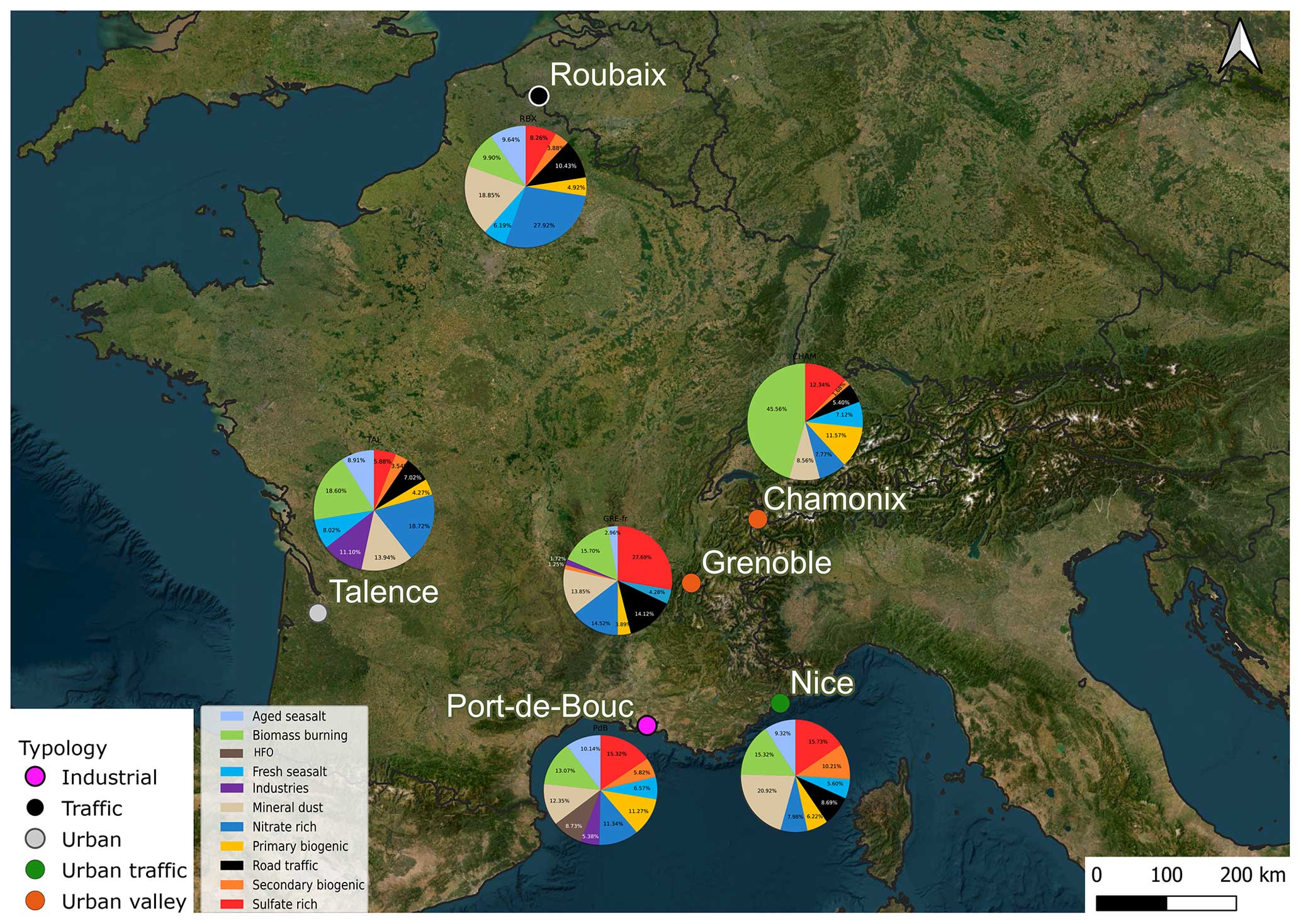
Figure 2 The location of the sites selected for this study. The small colored dots represent the typology of the sites. The pie charts are the PM₁₀ source apportionment for each site with the colors identifying the PM₁₀ sources. Background photography from ESRI satellite imagery.

Table 1 Data description.

2.3 OP analysis

PM₁₀ OP assays were performed on PM₁₀ extracted from the filters using simulated lung fluid, as detailed in Calas et al. (2017, 2018). The AA assay involved ascorbic acid, a natural antioxidant in the lungs inhibiting lipid and protein oxidation in the lining fluid, using the method presented by Kelly and Mudway (2003) and further described by Calas et al. (2018). Conversely, the DTT assay used dithiothreitol (DTT) as a chemical surrogate for cellular reducing agents, specifically nicotinamide adenine dinucleotide and nicotinamide adenine dinucleotide phosphate oxidase, thereby replicating in vivo interactions between PM₁₀ and biological oxidants (Cho et al., 2005; Calas et al., 2018). Both assays measured the consumption of AA or DTT during the assay, i.e., the rate of the transfer of electrons from AA or DTT to oxygen. The assays were conducted with 96-well plates of UV-transparent quality (CELLSTAR, Greiner Bio-One), and absorption measurements were acquired using a TECAN spectrophotometer (Infinite M200 Pro) at the wavelengths of 265 nm for the AA assay and 412 nm for the DTT assay (Calas et al., 2017, 2018, 2019). Each sample extraction was subjected to four analyses; the PM₁₀ OP in this study represents the mean and the analysis uncertainty is the standard deviation of these four PM₁₀ OP analyses. After analysis, the PM₁₀ OP activities of each sample were blank-subtracted using laboratory and field blanks, and normalized using the air sampling volumes and the mass concentration. The resulting OP_V represents the PM₁₀ OP due to PM₁₀ per cubic meter of air (nmol min⁻¹ m⁻³). To simplify the denotation of PM₁₀ OP, OP is used to represent PM₁₀ OP throughout this article.

2.4 Collinearity and heteroscedasticity tests

The result of a regression model strongly depends on the characteristics of the dataset because each model makes assumptions about the data. Two critical assumptions in OLS regression analysis are that (1) there is little collinearity between independent variables (the PM₁₀ sources in this study) and (2) the variance of the regression residuals is constant (called “homoscedasticity”). These assumptions should be tested in different ways.

2.4.1 Collinearity

Collinearity occurs when one or more of the independent variables is close to a linear combination of the other independent variables. When collinearity is present, small changes in the data can cause large changes in estimated coefficients, and the estimated standard errors of the coefficients are large. The variance inflation factor (VIF) is an indicator of the collinearity between independent variables (Craney and Surles, 2002; O'Brien, 2007; Rosenblad, 2011). The VIF of a specific source is calculated as

$$\begin{array}{}\text{(1)}& {\mathrm{VIF}}_i={\displaystyle \frac{\mathrm{1}}{\mathrm{1}-R_i^{\mathrm{2}}}},i=\mathrm{1},\mathrm{\dots },p-\mathrm{1},\end{array}$$

where p is the number of PM₁₀ sources and R² is the coefficient of determination of a multiple linear regression model between the ith source and the other sources. The VIF values of a PM₁₀ source present a range between 1 and ∞. The higher the VIF values, the greater the collinearity between this PM₁₀ source and the other sources. A VIF value between 5 and 10 is commonly interpreted as moderate collinearity, while values greater than 10 indicate high collinearity (Craney and Surles, 2002).

2.4.2 Heteroscedasticity

Heteroscedasticity occurs when the variance of regression residuals is not constant but varies for different values of the dependent variable. In this case, the estimated standard errors of the regression coefficients are not reliable. The Goldfeld–Quandt test was developed by Goldfeld and Quandt (1965) to evaluate residual variance in a regression model. To implement the Goldfeld–Quandt test, an OLS regression was performed between OP and PM₁₀ sources to identify the residual of OP prediction. Next, the PM₁₀ sources and corresponding residual are divided into three segments: the upper segment is the group with higher PM₁₀ source concentration, the lower segment is the group with lower PM₁₀ source concentration, and the middle segment, constituting 10 % of the moderate PM₁₀ concentration, is excluded. A subsequent regression analysis is then conducted on the two remaining subgroups to determine the ratio of residual sums of squares. Finally, an F test is conducted on this ratio to assess whether the variances are the same, with a p value below 0.05 interpreted as evidence of heteroscedasticity.

The variance inflation factor (VIF) and the Goldfeld–Quandt test were performed in Python 3.9, using the statsmodels 0.14.0 package (Seabold and Perktold, 2010).

2.5 Regression models

The fundamental principle of regression models in this study is to use the PM₁₀ sources to predict OP activities by identifying the parameters (coefficients and residuals) that minimize an error term (Hastie, 2009). A simple regression model can be represented by Eq. (2), which defines the estimated function of the regression model, and by Eq. (3), which estimates the residuals:

$$\begin{array}{}\text{(2)}& {\displaystyle }\widehat{y}=f\left(X\right)+e,\text{(3)}& {\displaystyle }e=y-\widehat{y},\end{array}$$

where $\widehat{y}$ is the estimated OP (nmol min⁻¹ m⁻³), X is the PM₁₀ source contribution (µg m⁻³), y is the observed OP (nmol min⁻¹ m⁻³), and e denotes the residuals (nmol min⁻¹ m⁻³). Each model has certain assumptions and a minimization term, as presented in the next section.

2.5.1 Ordinary least squares (OLS)

OLS is a linear regression technique that minimizes the residual sum of squares. This model is based on several assumptions: (1) linearity – the relationship between OP and PM₁₀ sources is linear; (2) independence – the PM₁₀ sources must be independent, with no collinearity; (3) homoscedasticity – the variance of residuals is constant across all values of PM₁₀ sources; and (4) normality – the residuals are normally distributed. In the OLS model, the estimated equation and objective to minimize are defined as follows:

$$\begin{array}{}\text{(4)}& {\displaystyle }\widehat{y}={\mathit{\beta }}_{\mathrm{0}}+\sum _{\mathrm{1}}^p{\mathit{\beta }}_i\cdot x_i,\text{(5)}& {\displaystyle }\mathrm{Minimize}\sum _{i=\mathrm{1}}^m{\left(y_i-\widehat{y_i},\right)}^{\mathrm{2}}\end{array}$$

where β₀ denotes the intercept (nmol min⁻¹ m⁻³), β_i represents the regression coefficient (intrinsic OP, nmol min⁻¹ µg⁻¹) of source i, x_i is the concentration of source i (µg m⁻³), p is the number of PM₁₀ sources, and m is the number of observations.

2.5.2 Weighted least square (WLS)

The assumptions and the minimization term in WLS closely align with those in OLS. The only difference is that WLS accounts for heteroscedasticity by introducing a weighting term for individual OP observations whose variance is assumed to be related to the variance of the residuals. The estimation equation in WLS is the same as that of OLS, but the objective to minimize is expressed as

$$\begin{array}{}\text{(6)}& \begin{array}{rl}& \mathrm{Minimize}\sum _{i=\mathrm{1}}^m{\left(y_i-\widehat{y_i}\right)}^{\mathrm{2}}\cdot w_i,\\ & w_i={\displaystyle \frac{\mathrm{1}}{{\mathrm{SD}}_i^{\mathrm{2}}}},\end{array}\end{array}$$

where w_i is the weight assigned to each observation and SD_i is the OP analysis variance of each observation.

2.5.3 Positive least squares (PLS)

The assumptions for PLS primarily include linearity, independence, and normality. PLS can be applied with weighting if there is heteroscedasticity in the data. PLS extends OLS with the constraint that the regression coefficients must be non-negative. The estimation equation and the error term, PLS, are similar to OLS (without weighting) and WLS (applying weighting). To ensure the positivity of coefficients, a specific condition must be met.

$$\begin{array}{}\text{(7)}& {\mathit{\beta }}_i\ge \mathrm{0},\forall i\mathrm{in}\mathrm{PM}\mathrm{sources}\end{array}$$

2.5.4 Ridge

Shrinkage methods such as Ridge regression try to produce a more interpretable model or reduce error in the presence of collinearity by selecting a subset of the independent variables. Ridge regression is introduced by Hoerl and Kennard (1970), and it incorporates a penalty term that shrinks the coefficients towards 0. Ridge regression minimizes the residual sum of squares plus a penalty term proportional to the sum of squares of the coefficients (L2 regularization) as shown in Eqs. (8) and (9). Consequently, Ridge regression reduces the influence of a PM₁₀ source that exhibits minimal impact on OP prediction without excluding it from the model.

$$\begin{array}{}\text{(8)}& {\displaystyle }\mathrm{Minimize}\sum _{i=\mathrm{1}}^m{\left(y_i-\widehat{y_i}\right)}^{\mathrm{2}}+\mathit{\lambda }\cdot \sum _{j=\mathrm{1}}^p{\mathit{\beta }}_j^{\mathrm{2}}\text{(9)}& {\displaystyle }\mathrm{Minimize}{\displaystyle \frac{\mathrm{1}}{\mathrm{2}m}}\sum _{i=\mathrm{1}}^m{w}_i{\left(y_i-\widehat{y_i}\right)}^{\mathrm{2}}+\mathit{\lambda }\cdot \sum _{j=\mathrm{1}}^p{\mathit{\beta }}_j^{\mathrm{2}}\end{array}$$

Here, λ is the parameter representing the amount of shrinkage; the larger λ, the greater the shrinkage. The hyperparameter tuning was implemented with different values of λ (5, 1, 0.5, 0.1, 0.01, 0.005, 0.001, 0.0005, and 0.0001). The best λ for every site varied from 0.005 to 0.01, and in this study, 0.01 was selected. Ridge can be applied with weighting to account for heteroscedasticity.

2.5.5 Least absolute shrinkage and selection operator (Lasso)

Lasso (Tibshirani, 1996) is a shrinkage method that uses a penalty term proportional to the sum of the absolute regression coefficients (L1 regularization). This penalty term shrinks the coefficients of a source with a low impact on OP prediction to 0, effectively removing it from the model. This results in a sparse model that may be easier to interpret and may reduce error on out-of-sample data. However, Lasso is more sensitive to outliers than Ridge regression and is less stable when data are collinear. Lasso can be applied with weighting to account for heteroscedasticity.

$$\begin{array}{}\text{(10)}& {\displaystyle }\mathrm{Minimize}\sum _{i=\mathrm{1}}^m{\left(y_i-\widehat{y_i}\right)}^{\mathrm{2}}+\mathit{\lambda }\cdot \sum _{j=\mathrm{1}}^p\left|{\mathit{\beta }}_j\right|\text{(11)}& {\displaystyle }\mathrm{Minimize}{\displaystyle \frac{\mathrm{1}}{\mathrm{2}m}}\sum _{i=\mathrm{1}}^m{w}_i{\left(y_i-\widehat{y_i}\right)}^{\mathrm{2}}+\mathit{\lambda }\cdot \sum _{j=\mathrm{1}}^p\left|{\mathit{\beta }}_j\right|\end{array}$$

Similar to Ridge, λ is the parameter representing the amount of shrinkage;  λ is selected as 0.01 in this study by running the hyperparameter tuning using the same values as for Ridge.

2.5.6 Generalized linear model (GLM)

Generalized linear models, as introduced by McCullagh (1989), provide a framework for regression analysis that can contain non-normal error distributions and capture non-linear relationships between OP activities and PM₁₀ sources. GLMs allow for error variance that is a function of the predicted value, hence accounting for heteroscedasticity. Key assumptions underlying GLM include (1) independence, (2) the non-normal distribution of OP, and (3) that the relationship between the PM₁₀ sources and the transformed OP (logarithm in this study) is linear. The mathematical expression for GLM can be represented as follows:

$$\begin{array}{}\text{(12)}& \log \left(\widehat{y}\right)={\mathit{\beta }}_{\mathrm{0}}+\sum _{\mathrm{0}}^p{\mathit{\beta }}_i\cdot x_i,\end{array}$$

where β₀ denotes the intercept, β_i represents the regression coefficient of source i, and x_i is the concentration of source i.

2.5.7 Random forest (RF)

RF, an ensemble learning method introduced by Breiman (2001), combines multiple decision trees to make predictions. In the reference implementation, each tree is grown on a bootstrap sample of the data, and a random subset of the available features is evaluated at each node to choose the best split. The predictions of all trees are averaged to give the RF final prediction. RF is customizable via hyperparameters such as the number of trees, the size of the bootstrap sample, and the number of features to evaluate at each node. For hyperparameter tuning, 5-fold cross-validation was used on the training data. The training dataset was separated into five parts: four parts were used for training and the remaining part was used for validation. This process was repeated five times, and the hyperparameter value producing the lowest mean RMSE across the five parts was selected. The hyperparameter tuning is shown in Sect. S1.1 in the Supplement.

RF does not assume a specific equation to express the relationship between OP activities and PM₁₀ sources, with the result that intrinsic OP could not be computed in this regression model. Nevertheless, RF can estimate the relative importance of each PM₁₀ source in OP prediction. This study estimated the permutation importance of each PM₁₀ source as the mean increase in the mean squared error of predicted OP when the values of the PM₁₀ source were permuted.

2.5.8 Multilayer perception (MLP)

MLP is an artificial neural network that consists of multiple layers of interconnected nodes or neurons organized in a feedforward structure (Akhtar et al., 2018; Chianese et al., 2018; Bourlard and Wellekens, 1989). These layers include an input layer (PM₁₀ sources), one layer or several hidden layers, and an output layer (OP_AA or OP_DTT activities). In MLP, the neurons in the hidden layers are linked to the previous neurons by the connection weight, where every neuron is independent and has a different weight. The output of each neuron depends on its inputs and an activation function, which, if non-linear, allows the model to capture non-linear relationships. The implementation of MLP includes three steps: (1) forward pass to training model – the input is passed to the model, multiplied with an initial weight, bias is added at every layer, and the output of the model is then calculated; (2) error calculation – after applying step 1, the output of the model and the observed data are used to calculate the error; (3) backward pass – the error is propagated back through the network, and the weights are then adjusted to minimize overall error. These three steps are repeated until the error is minimized.

The choice of hyperparameters to ensure the MLP model robustness is processed by hyperparameter tuning using 5-fold cross-validation, as shown in Sect. S1.2. Thanks to hyperparameter tuning, the two hidden layers and a logistic sigmoid activation function were selected in this study to capture the non-linear relationships between OP activities and PM₁₀ sources.

All regression models were performed using the Python package statsmodels 0.14.0 (Seabold and Perktold, 2010) and scikit-learn 1.3.1 (Pedregosa et al., 2011).

2.5.9 Performance of the models

The performance metrics R-square (R²), mean absolute error (MAE), and root mean square error (RMSE) were used to assess the goodness of fit of the models, as described by Kuhn and Johnson (2013). R² quantifies the ability of the model to explain the variance in the data. R² = 1 indicates a perfect fit. RMSE represents the aggregation of the individual differences between predicted OP and measured OP, while MAE assesses the average magnitude of errors between them. Lower RMSE and MAE values indicate a better fit, with a perfectly fitting model yielding an RMSE or MAE of 0. Equations (13), (14), and (15), respectively, define R², MAE, RMSE. These indicators are computed for the training and testing data of each sampling iteration and averaged across the 500 sampling iterations.

$$\begin{array}{}\text{(13)}& {\displaystyle }\begin{array}{rl}{R}^{\mathrm{2}}& =\mathrm{1}-{\displaystyle \frac{\mathrm{Sum}\mathrm{of}\mathrm{Squared}\mathrm{Residuals}}{\mathrm{Total}\mathrm{Sum}\mathrm{of}\mathrm{Squares}}}=\mathrm{1}\\ & -{\displaystyle \frac{{\sum }_{i=\mathrm{0}}^m{\left(y_i-\widehat{y_i}\right)}^{\mathrm{2}}}{{\sum }_{i=\mathrm{0}}^m{\left(y_i-\widehat{y_i}\right)}^{\mathrm{2}}}}\end{array}\text{(14)}& {\displaystyle }\mathrm{MAE}={\displaystyle \frac{{\sum }_{i=\mathrm{0}}^m\left|y_i-\widehat{y_i}\right|}{m}}\text{(15)}& {\displaystyle }\mathrm{RMSE}=\sqrt{{\displaystyle \frac{{\sum }_{i=\mathrm{0}}^m{\left(y_i-\widehat{y_i}\right)}^{\mathrm{2}}}{m}}}\end{array}$$

3 Result and discussion

Assessments of collinearity and homoscedasticity are addressed in Sect. 3.1. Model performance, including key performance metrics and identification of the optimal model, is detailed in Sect. 3.2. Section 3.3 compares the intrinsic OP estimated by the different models. Section 3.4 compares the intrinsic OP between the combined best-fit and reference models. Lastly, Sect. 3.5 proposes recommendations for selecting an appropriate model.

3.1 Dataset characteristics

The contributions of identified sources (µg m⁻³) and the OP_v activities (nmol min⁻¹ m⁻³) in each site are presented in Fig. 3, illustrating variations in annual average OP activities and PM₁₀ source contributions by site. Most sites, including traffic and industrial sites, show higher OP_DTT activities than OP_AA. Conversely, for the alpine valley sites, CHAM presents higher OP_AA than OP_DTT, while GRE-fr experiences similar levels of OP_AA and OP_DTT. Additionally, the average OP activities in every site are not proportional to the average PM concentration. For instance, CHAM and NIC had lower PM₁₀ concentrations but higher OP activities than other sites, while TAL showed high PM₁₀ concentrations but relatively lower OP activities.

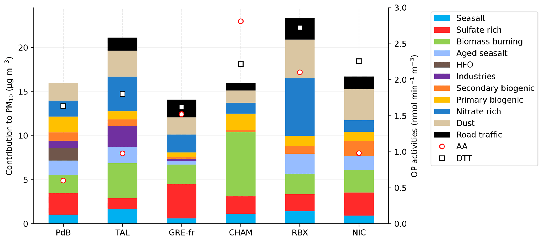
Figure 3 The contribution of sources to PM₁₀ and the OP activities in six sites. The left y axis and bar show the contribution of PM sources in µg m⁻³. The right y axis, circles, and squares show the mean OP_v activities in nmol min⁻¹ m⁻³, with the red circle indicating OP_AA and the black square indicating OP_DTT.

The variations observed in the levels of PM₁₀ and OP across six sites can be attributed to distinctions in the identified sources and their respective contributions. These disparities are contingent upon the unique typologies of each site, which are discussed in Weber et al. (2021). Further, we can observe a significant seasonality in the OP activities (Table S1 in the Supplement). The strong seasonality of OP in alpine valley sites has been addressed in previous studies (Borlaza et al., 2021; Dominutti et al., 2023; Weber et al., 2018, 2021), with thermal inversions during winter increasing pollutant concentrations and OP activities compared with summer. Conversely, OP activities in cold and warm periods in other sites are not significantly different.

The PM₁₀ sources and their distribution vary among sites (Fig. 3) because of the difference in typology and local activities. For instance, in the industrial site (PdB), two specific sources are identified: shipping emissions (HFO), with an annual mean contribution of 1.39 µg m⁻³, and industrial sources at 0.86 µg m⁻³. The urban background site TAL also appears to be influenced by industrial sources (2.34 µg m⁻³), which might, however, be partly due to biases induced by the application of the harmonized receptor model protocol (Weber et al., 2019). Note that the application of a site-specific PMF procedure for this site leads to a much lower contribution of this source category but relatively similar contributions of other sources (Favez, 2017). GRE-fr, an urban background site in an alpine valley, presents significant long-range transport sources, with secondary sulfate contributing 3.90 µg m⁻³ followed by biomass burning at 2.21 µg m⁻³. As expected, biomass burning is an abundant source in CHAM, accounting for 7.28 µg m⁻³ of the PM contribution, while the traffic sites RBX and NIC displayed high contributions of traffic sources (at 2.43 and 1.45 µg m⁻³, respectively).

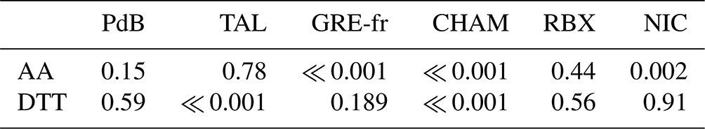
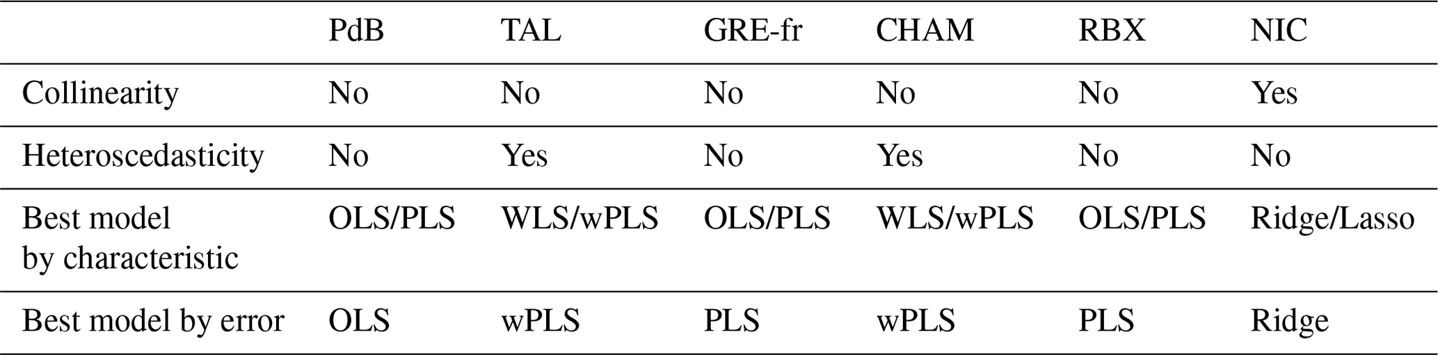
The presence of multicollinearity and homoscedasticity was tested to assess the data characteristics of every site. The only site with evidence of collinearity was NIC, where the VIF of the traffic source was equal to 5.0. For all other sites, VIF values are below 5, indicating limited collinearity among sources. This is expected, as the PMF analysis is constrained to avoid collinearity between sources. VIF values for each site can be found in Table S2.

The presence of heteroscedasticity is commonly found when the dependent variable (or OP in this study) exhibits a large difference between the minimum and maximum values or when the error variance varies proportionally with an independent variable (PM₁₀ sources). The heteroscedasticity was assessed by applying the Goldfeld–Quandt test. Table 2 presents the p values of the Goldfeld–Quandt test, indicating homoscedasticity of OP prediction when p>0.05. This test reveals that heteroscedasticity was detected in CHAM, in GRE-fr, in NIC for OP_AA, and in CHAM and TAL for OP_DTT (Table 2). We observed a large difference between the cold and warm periods for both OP_AA and OP_DTT in CHAM, similar to what was seen for OP_AA in GRE-fr (Table S1), which can be the reason for the presence of heteroscedasticity. For NIC and TAL, there is an insignificant difference between the cold and warm periods, which indicates the presence of heteroscedasticity may be because of the relationship between the PM₁₀ sources and error variance. When heteroscedasticity is detected, unweighted regression for OP prediction according to the source may not accurately reflect the uncertainty in the intrinsic OP of each source. The scatterplots representing the relationship between the regression analysis residuals and the fitted values (for observed OP) are available in Figs. S1 and S2 in the Supplement.

Table 2 The p value of the Goldfeld–Quandt heteroscedasticity test.

3.2 Performance of regression models

The 11 regression models, with or without the weighting for some of them, were tested by comparing their performance metrics between the measured and reconstructed OPs. For each run (n=500 iterations), the R², RMSE, and MAE were computed for the testing and training dataset, resulting in 500 values for each performance metric. Figure 4 presents the mean R² values of the training datasets as well as the mean and the standard deviation of the testing datasets of the OP_AA models across the 500 sampling iterations, and Fig. 5 presents the mean RMSE and MAE. The same result pattern was found for OP_DTT, as presented in Tables S3, S4, S5. The WLS, wPLS, wRidge, and wLasso models incorporated weighting, while the OLS, PLS, Ridge, Lasso, GLM, RF, and MLP models were unweighted.

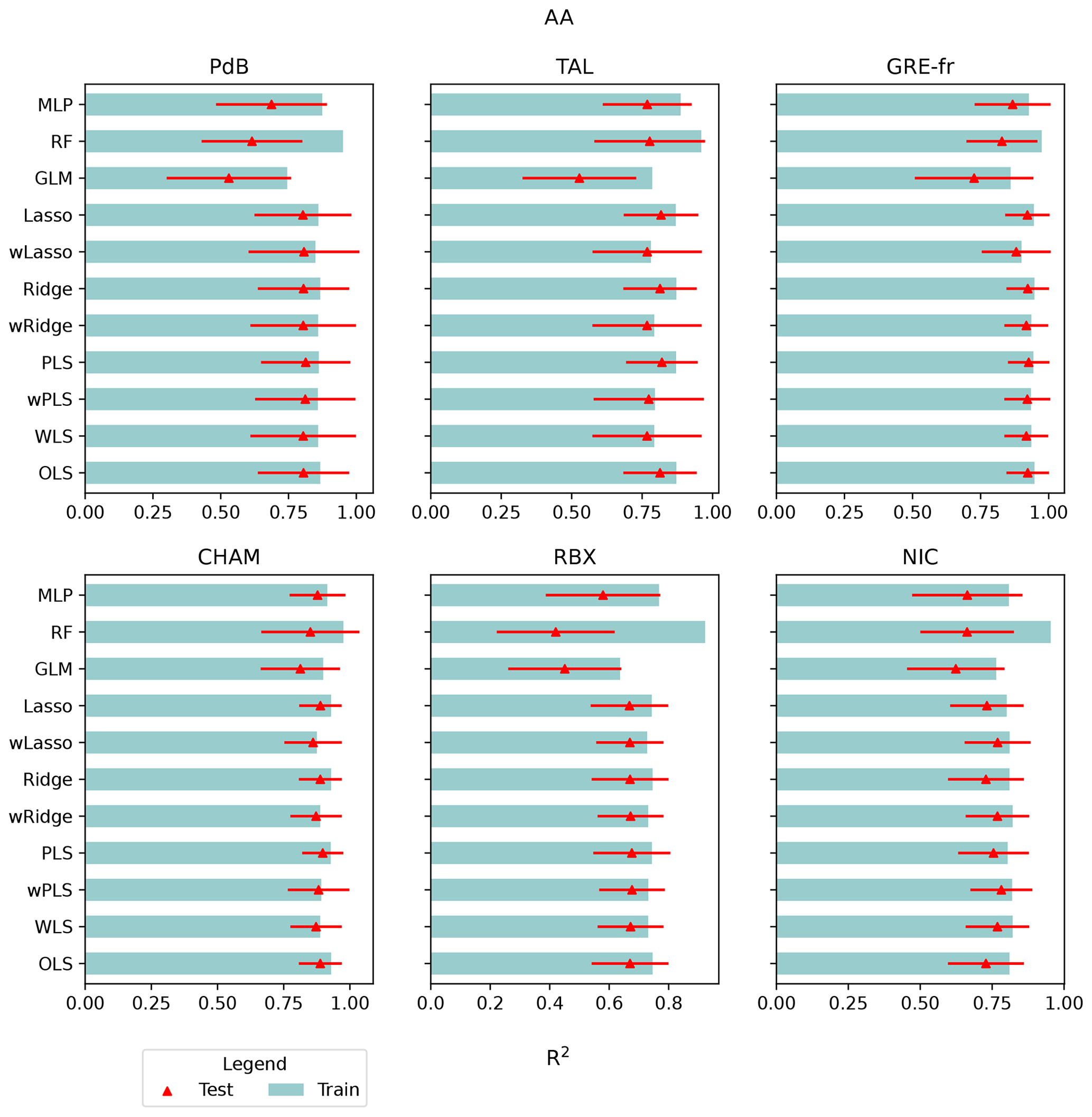
Figure 4 The R² values of 11 OP_AA models in six sites. The mean R² of the training data is shown by the blue bars, the mean R² of the testing data is shown by the red triangled, and the standard deviation of the R² of the testing data is shown by the red bars. The y axis represents the models, and the x axis denotes the R² values.

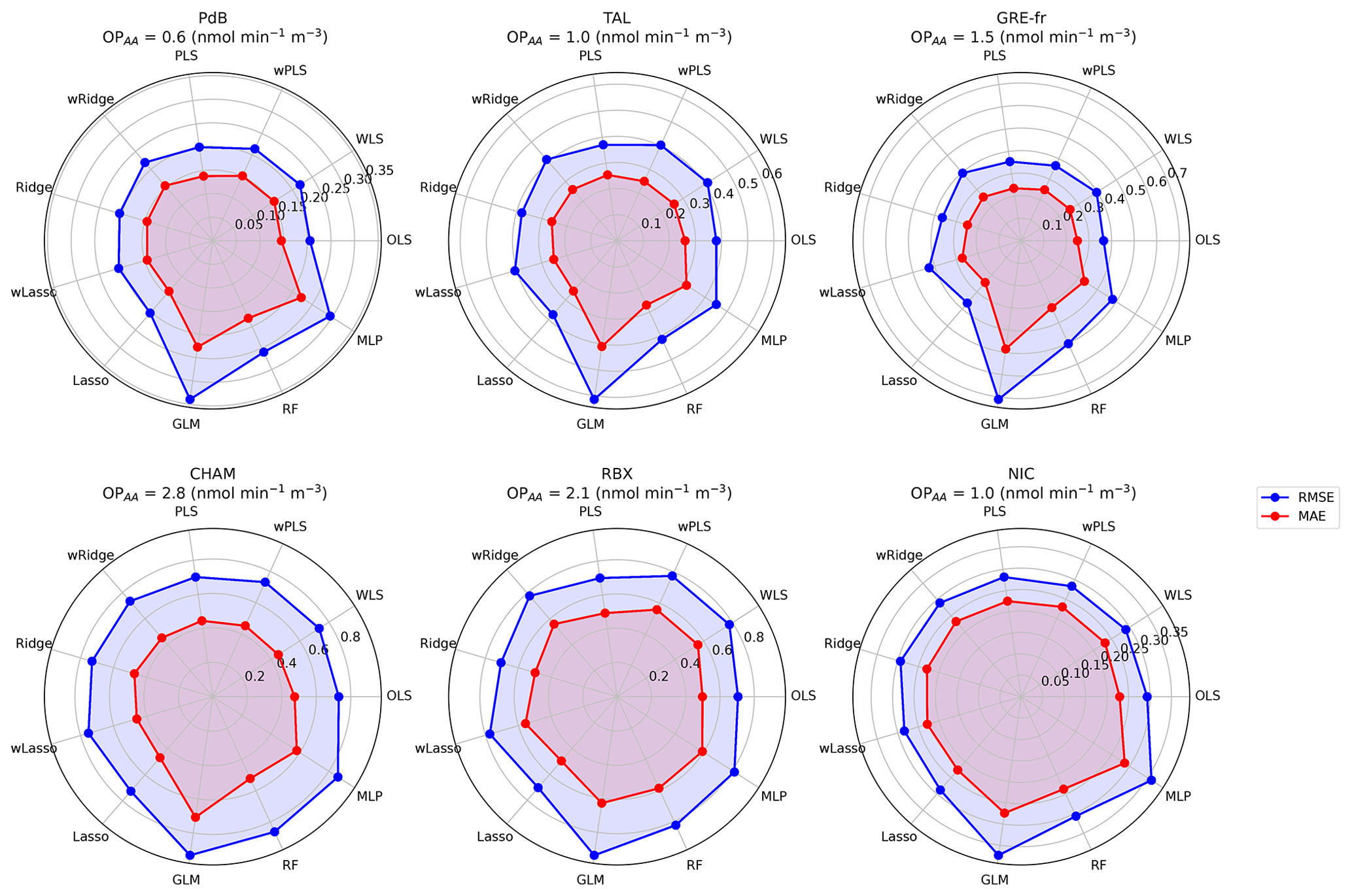
Figure 5 The MAE and RMSE of 11 OP_AA models in every site for the testing data. Blue and red lines represent the RMSE and the MAE, respectively. The values in the figure are the mean of the RMSE and MAE of 500 iterations.

OP predictions across all sites are statistically validated, with testing R² values in RBX, NIC, PdB, TAL, CHAM, and GRE-fr observed to be 0.66, 0.76, 0.76, 0.78, 0.87, and 0.90, respectively. The lowest mean test set RMSE values are 0.70, 0.28, 0.21, 0.37, 0.70, and 0.31 nmol min⁻¹ m⁻³, respectively, for the same sites. The lowest mean test set MAE values are 0.49, 0.23, 0.14, 0.25, 0.45, and 0.21 nmol min⁻¹ m⁻³, respectively. Notably, the GLM model exhibits the lowest R² values and the highest RMSE for all sites (Tables S3–S5). These results strongly suggest that the relationship between OP_AA and PM₁₀ sources is not log-linear.

Differences in MAE, RMSE, and R² between the training and testing database for RF and MLP are significant across the sites. Notably, RF displays a large difference in R² , with a gap of up to 0.6 in RBX (R² training: 0.92; R² testing: 0.27). Similar gaps were found in RMSE and MAE. RF consistently performed best on the training set, characterized by the highest R² and the lowest MAE and RMSE values, but had lower test set R² values than the other models (except GLM). Conversely, MLP exhibited training R² values comparable to other models but lower test R² values. These findings suggest overfitting: the flexible algorithms identify relationships in the training data that do not generalize to the testing data. This observation may be attributed to the limitations of data coverage, possibly failing to fully represent the underlying relationships, leading to poor performance in the testing datasets (Matsuki et al., 2016; Benkendorf and Hawkins, 2020; Stockwell and Peterson, 2002; Wisz et al., 2008; Hernandez et al., 2006; Hawkins, 2004; Raudys and Jain, 1991). Pearce and Ferrier (2000) recommended that the minimum number of samples for robust performance should be over 250 for GLM model, while Raudys and Jain (1991) showed that the minimum number of samples is based on the complexity of the model and the number of predictors. Additionally, Harrell (2016) suggested that the number of predictors (PM sources) should be below the number of samples divided by 15, a threshold not reached in this analysis. For example, in NIC, the minimum number of samples should be 135 for the training set (9 PM sources × 15), while in total, we have only 107 samples. Therefore, we can also recommend that, for optimal performance of RF and MLP, the number of samples and PM sources should satisfy these thresholds.

The WLS, OLS, wPLs, wRidge, and wLasso models show more robust performances with fewer differences between the training and testing data. At most sites, there is very little difference between the R², RMSE, and MAE of OLS and Ridge, with or without weighting, and often between PLS and Lasso as well. This consistency is observed even in the collinearity case of NIC, where VIF = 5. The difference between these models is a maximum of 0.06 in R², 0.01 in MAE, and 0.1 in RMSE, indicating that these models work well for OP prediction. Nevertheless, it is worth noting that every model exhibits different assumptions that have to be respected. The assumption violations may lead to unreliable regression coefficients (intrinsic OP) even though the prediction is good (Williams et al., 2013; Cohen et al., 2002).

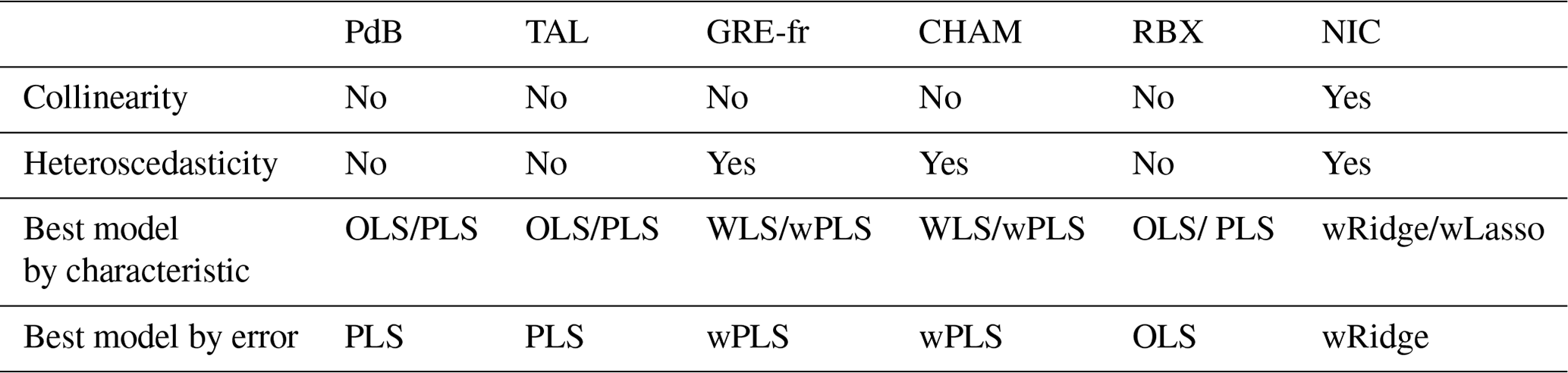
The best model for each site was selected based on both data characteristics (collinearity and heteroscedasticity) and testing data performance. For sites with collinearity, Ridge and Lasso were considered the most appropriate. For sites with heteroscedasticity, models with weights were considered the most appropriate. For sites with neither collinearity nor heteroscedasticity, OLS and PLS were considered the most appropriate. Tables 3 and 4 present the best OP_AA and OP_DTT prediction models for each site. It follows that the best model is not necessarily the same one for both series of OP for a given site. As a rule, the model that exhibits the best performance metrics (the best model by error in Table 3 for OP_AA and Table 4 for OP_DTT) is suited to be the best model chosen by data characteristics; therefore, choosing a model according to data characteristics help to obtain more reliable OP predictions.

Table 3 Criteria for selection of the best model for OP_AA.

Table 4 Criteria for selection of the best model for OP_DTT.

3.3 Effect of the choice of a model on intrinsic OP

It is particularly important to try to define the best way of calculating the more accurate intrinsic OP of PM sources and the contribution of sources to OP, since these values are fundamental inputs in all the works of large-scale modeling of OP with chemical transport models (CTM) (Daellenbach et al., 2020; Vida et al., 2024). Figures 6 and 7 show the variations in intrinsic OP for all the models, focusing on the results of NIC as an example. The evaluation of the five other sites is presented in Figs. S3–S7 for OP_AA and Figs. S8–S12 for OP_DTT. The differences in equations, error term minimizations, and assumptions can explain the differences in intrinsic OP per µg of source among the eight regression models. While the R² , RMSE, and MAE values are similar among models (except for GLM, RF, and MLP), the intrinsic OP values significantly differ between the models with and without weighting and between the linear and non-linear regression models. The average intrinsic OP of 500 iterations is discussed in this section, since these values are generally used to calculate the contribution of the PM₁₀ source to OP in prior studies (Borlaza et al., 2021; Dominutti et al., 2023; Weber et al., 2018). The mean and standard deviation of intrinsic OP_AA and OP_DTT for the six sites are shown in Tables S6 and S7, respectively.

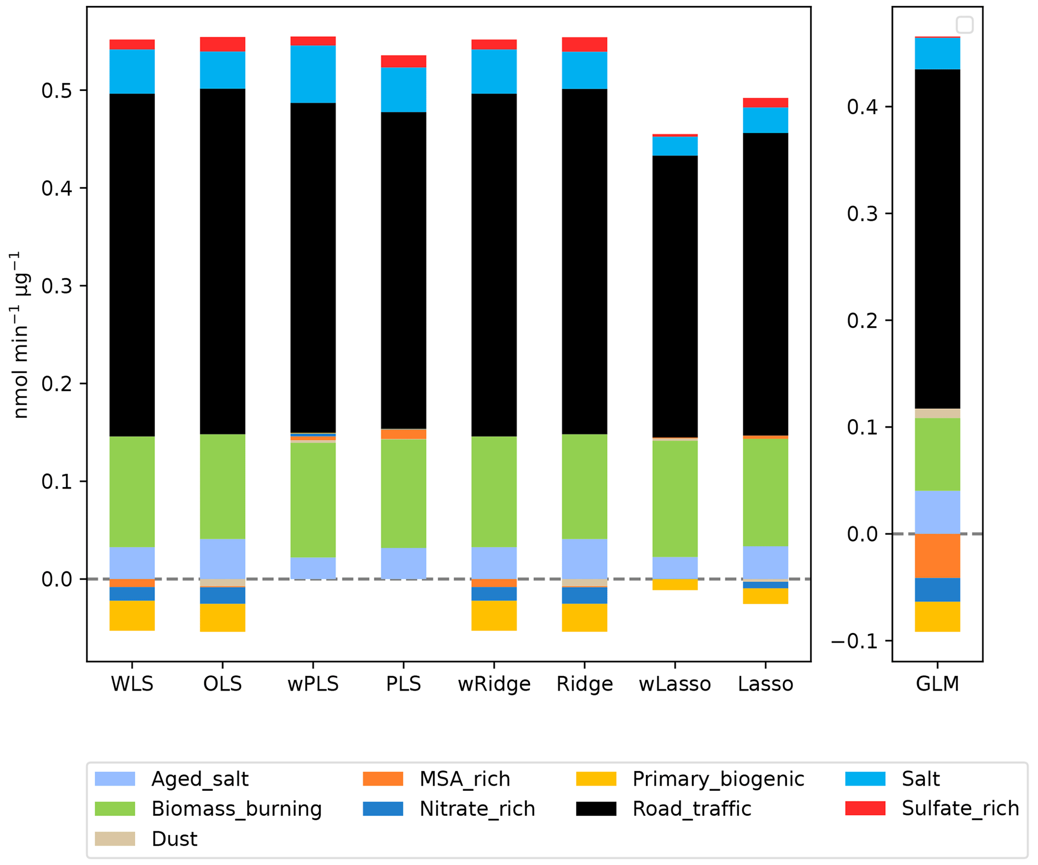
Figure 6 Intrinsic OP_AA values of the different PM₁₀ sources at Nice obtained with the different models.

The intrinsic OP_AA of PM₁₀ sources at NIC is the same between WLS and wRidge and between the OLS and Ridge, revealing that the moderate collinearity of the road traffic source did not affect the estimated intrinsic OP_AA. PLS sets the intrinsic OP_AA of some sources to 0, therefore producing slightly different results. Lasso regression sets the intrinsic OP_AA of some sources to 0 and shrinks the estimates for all other sources toward 0. GLM produces intrinsic OP_AA values that represent a multiplicative change on the log scale, and thus they are not directly comparable to the other models. However, the direction and importance of the sources are similar to the other models. Whatever the model, road traffic appears as the source with the highest intrinsic OP_AA, followed by biomass burning, aged salt, salt, and sulfate-rich sources, in NIC. Traffic and biomass burning sources have been similarly recognized as significant contributors to OP_AA in prior studies (Borlaza et al., 2021; Dominutti et al., 2023; Stevanović et al., 2023). The intrinsic OP of the dominant sources is stable, indicating that all these models could give the same information about the intrinsic OP of the main sources. Conversely, the differences are larger between models for the sources with small to very small intrinsic OP (MSA-rich, primary biogenic, nitrate-rich, and dust sources), whose intrinsic OP varies from positive to negative among models.

The OP_DTT intrinsic values in NIC (Fig. 7) display minimal variation among the WLS and wPLS. This consistency is linked to the absence of negative intrinsic values. On the other hand, even though there is the presence of moderate collinearity, wRidge still has the same result as WLS and wPLS. In line with the OP_AA results, the wLasso and GLM models exhibit distinct responses compared with the other models. The intrinsic OP_DTT of all sources varies depending on the presence or absence of weighting. While the WLS models tend to amplify the influence of some sources (aged sea salt, primary biogenic, sea salt, and sulfate-rich sources), the OLS reduces the intrinsic OP_DTT of these sources. Conversely, MSA-rich, nitrate, and road traffic sources undergo less influence in WLS but more influence in OLS. Different from OP_AA, OP_DTT prediction shows more variation among models, highlighting the effect of choosing a model on evaluating the intrinsic OP_DTT of PM₁₀ sources.

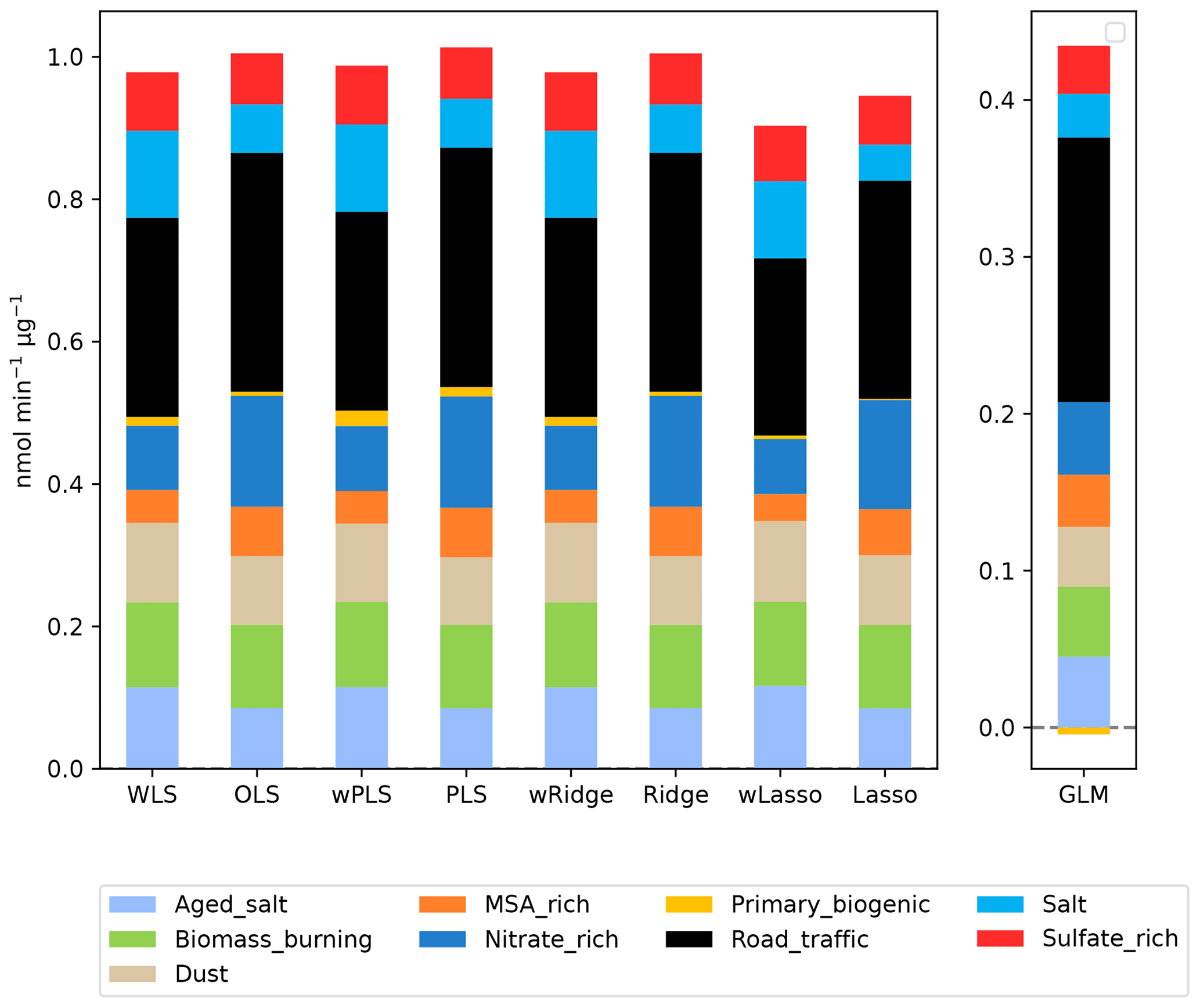
Figure 7 Variations in the intrinsic OP_DTT of the different PM₁₀ sources at Nice obtained with the different models.

The comparison of intrinsic OP among regression models in NIC demonstrated that OP_DTT and OP_AA intrinsic values exhibit variation across different models with and without weighting, illustrating that the choice of the model significantly influences the values obtained for intrinsic OP of PM₁₀ sources (a similar pattern is observed for all other sites and shown in Figs. S3–S7 for OP_AA and Figs. S8–S12 for OP_DTT). Because of the difference in intrinsic OP across models, a comparison between the best-performing and most commonly used models (OLS) is presented in the following section to elucidate the advantage of choosing a model based on data characteristics (Sect. 3.4).

3.4 Comparisons between the best site-specific model and OLS

In this section, the intrinsic OP of the best model is selected for each site as discussed in Sect. 3.2, and the intrinsic values of each source are compared with the ones returned by the OLS model. The OLS model is used as a representative of usual practices that do not consider the database characteristics (Williams et al., 2013). The average intrinsic OP value of each PM₁₀ source is calculated from all 500 bootstrapping iterations for all sites where that particular source is identified. Intrinsic OP values obtained in this way from the best model (the best model presented in Table 3 for OP_AA and Table 4 for OP_DTT) encompassing all six sites are called “the intrinsic OP of the best model”, and the intrinsic OP values derived from the OLS from all six sites are called the “intrinsic OP of the reference model”.

A meaningful comparison of the two series of intrinsic values requires two conditions. First, intrinsic OP should be consistent across all sites. While recognizing that intrinsic OP values depend on diverse factors, we assumed the sites share fairly uniform PM₁₀ chemical source profiles in France. This is demonstrated by evaluating the Pearson distance and standardized identity distance similarity indicators of the source chemical profiles (Belis et al., 2015; Weber et al., 2019), and Fig. S13 indicates consistent profiles of sources for the six sites. Consequently, we could expect to observe minimal divergence in intrinsic OP values among these sites. Second, we postulate that negative intrinsic OP values are possible since previous studies have reported that total PM₁₀ intrinsic OP can be modulated due to the synergetic/antagonistic effects involving, for example, soluble copper, quinones, and bacteria (Borlaza et al., 2021; Pietrogrande et al., 2022; Samake et al., 2017; S. Wang et al., 2018; Xiong et al., 2017). Samake et al. (2017) demonstrated that the presence of bacterial cells in aerosol decreases the redox activity of Cu and 1,4-naphthoquinone, with a maximum decrease of 60 % compared with the oxidative reactivity considered individually. Pietrogrande et al. (2022) indicated that the mixture of Cu, Fe, 9,10-phenanthrene quinone, and 1,2-naphthoquinone reduces the rate consumption of AA and DTT by up to 50 % depending on the quantity of each chemical. Wang et al. (2018) reported that the mixing of Cu, naphthalene secondary organic aerosol (SOA), and phenanthrene SOA only achieved half of the DTT rate consumption compared with the separately considered consumption. Xiong et al. (2017) showed the presence of antagonists in the interaction of Fe and quinones; nevertheless, it was much lower than those in the other studies (under 10 %). These references reported that the antagonistic effects of a mixture can significantly reduce the consumption rate of OP_DTT and OP_AA, and this impact varies widely from 10 % to 60 % depending on the type of chemical species and the quantity of each species in the mixture. Consequently, we consider here that the intrinsic OP value of an individual site for a given source could be negative only within a range of at most 60 % of the mean combined intrinsic OP value of this source across all sites. Negative intrinsic OP exceeding this criterion may result from the mathematical construction of the model. The comparison between the intrinsic OP_AA of the best model and the reference model is presented in Sect. 3.4.1 and that of OP_DTT is shown in Sect. 3.4.2.

3.4.1 OP_AA activities

The results of the comparison of OP_AA intrinsic values (Fig. 8 and Table S8) show that the anthropogenic sources have the highest intrinsic OP values in both the best model and the reference model. Among these sources, road traffic appears as the most prominent potent fraction, followed by biomass burning, HFO, and industrial sources. These results are aligned with prior research (Calas et al., 2019; Daellenbach et al., 2020; Dominutti et al., 2023; Fadel et al., 2023; Fang et al., 2016; in't Veld et al., 2023; Weber et al., 2018; Zhang et al., 2020) which has highlighted the sensitivity of OP_AA to concentrations of metals, black carbon, and organic carbon. The differences between the best model and the reference model were insignificant for these sources, demonstrating that the best model and the reference model consistently captured similar patterns for the most critical sources of OP activities.

However, the interquartile ranges (IQR) of the intrinsic OP values are consistently narrower for the best model across all sources, accounting for less divergence in intrinsic OP values across sites. Moreover, the median intrinsic OP values obtained from the best model closely approximated the mean values, indicating the absence of extreme intrinsic OP values. For instance, in the case of road traffic, the mean and median values were 0.24 and 0.23 nmol min⁻¹ µg⁻¹, respectively. Conversely, the reference model exhibited a large difference between the mean and median values, implying lower consistency across sites and sampling iterations. The same result was observed in biomass burning source, in which the median and mean intrinsic OP in the best model had fewer discrepancies. Further, the biomass burning intrinsic OP in GRE-fr of the best model is more consistent with those in other sites (best: 0.30 nmol min⁻¹ µg⁻¹; reference: 0.35 nmol min⁻¹ µg⁻¹).

When considering sources with low intrinsic OP, the variability can be larger between the two methods. As an example, for the sulfate-rich sources, the median intrinsic OP values were positive (0.002 nmol min⁻¹ µg⁻¹), while the mean intrinsic OP values were negative (−0.008 nmol min⁻¹ µg⁻¹). The mean intrinsic OP in the best model exhibited fewer negative values in individual sites than in the reference model (for aged salt, salt, primary biogenic, MSA-rich, sulfate-rich, and nitrate-rich sources). In addition, the best model showed the least disparate intrinsic OP among individual sites, for instance, the aged salt sources in GRE-fr and the primary biogenic and salt sources in CHAM. Furthermore, the best model displayed an intrinsic OP meaningful in terms of geochemical validation, which was shown in the salt, primary biogenic, and sulfate-rich sources. For instance, in the reference model, the average intrinsic OP of the primary biogenic source in NIC (−0.03 nmol min⁻¹ µg⁻¹), the intrinsic OP of salt in GRE-ft (−0.07 nmol min⁻¹ µg⁻¹), and the sulfate-rich source in CHAM (−0.05 nmol min⁻¹ µg⁻¹) represented a 100 % reduction compared with the mean intrinsic OP of all sites. Moreover, negative intrinsic OP was observed in NIC (primary biogenic), and some extreme values were observed in GRE-fr (aged salt, salt) and CHAM (salt, primary biogenic, MSA-rich; where heteroscedasticity was presented) in the OLS model, which underscores that the model assumptions on data characteristics proving false could impact the accuracy of OP prediction. Consequently, these results highlight the advantage of considering the data in the model selection.

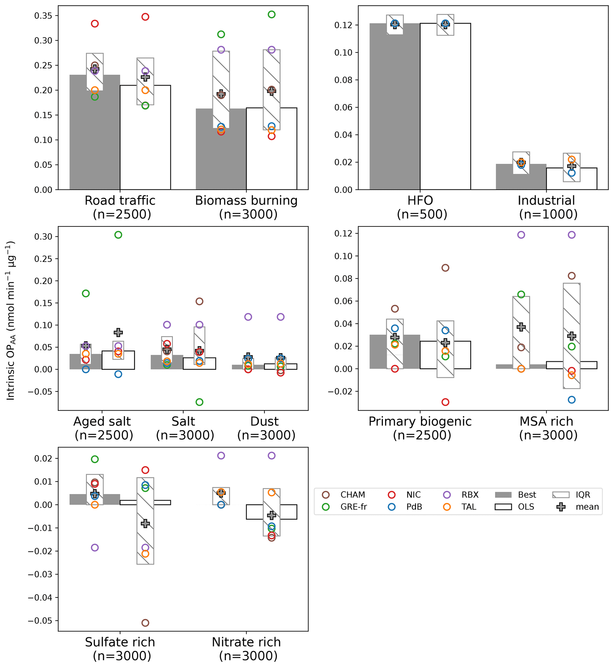
Figure 8 Intrinsic OP_AA estimated by the best model and the reference method in the six sites. The y axis represents the intrinsic OP values in nmol min⁻¹ µg⁻¹, and the x axis represents the sources. The gray bars are the median intrinsic OP values of the best models in the six sites (n=500 bootstrapping × number of sites where the given source is detected) for each source. The white bars are the same median intrinsic OP values for the reference (OLS) model. The gray plus symbol represents the mean of intrinsic OP values. The hatched bars are the interquartile ranges of the intrinsic OP values. The dots represent the mean intrinsic OP of all sites, including gray – Chamonix, green – Grenoble, red – Nice, blue – Port-de-Bouc, purple – Roubaix, and orange – Talence.

The detailed comparison of intrinsic OP_AA between the best model and the reference model is categorized into four groups and discussed in detail in Sect. S9. These groups include (1) anthropogenic sources without nitrate and sulfate (road traffic, biomass burning, HFO, and industrial sources); (2) natural inorganic sources (aged sea salt, sea salt, dust); (3) biogenic sources (primary biogenic and MSA-rich sources); and (4) nitrate and sulfate-rich sources.

3.4.2 OP_DTT activities

Similar to OP_AA, for OP_DTT the IQR of the best model is narrower for most of the sources than the IQR of the reference model (OLS). Except for road traffic, industrial, and MSA-rich sources, the IQR is slightly higher in the best model (Fig. 9 and Table S9). In the two models, the mean intrinsic OP is essentially unchanged, where traffic is the most critical source (0.27 ± 0.10) followed by HFO (0.18 ± 0.01), biomass burning (0.12 ± 0.03), dust (0.12 ± 0.07), primary biogenic (best: 0.10 ± 0.06; reference: 0.12 ± 0.08) and MSA-rich sources (best: 0.11 ± 0.09; reference: 0.09 ± 0.09). The minimum difference between the two models in the dominant sources again confirms the conclusion in the OP_AA comparison, demonstrating the similar pattern of the best model and the reference model in the most crucial sources of OP. For both the best and the reference models, OP_DTT activities showed sensitivity to more sources compared with OP_AA, as discussed in previous studies (Borlaza et al., 2021; Calas et al., 2019; Dominutti et al., 2023; Fadel et al., 2023).

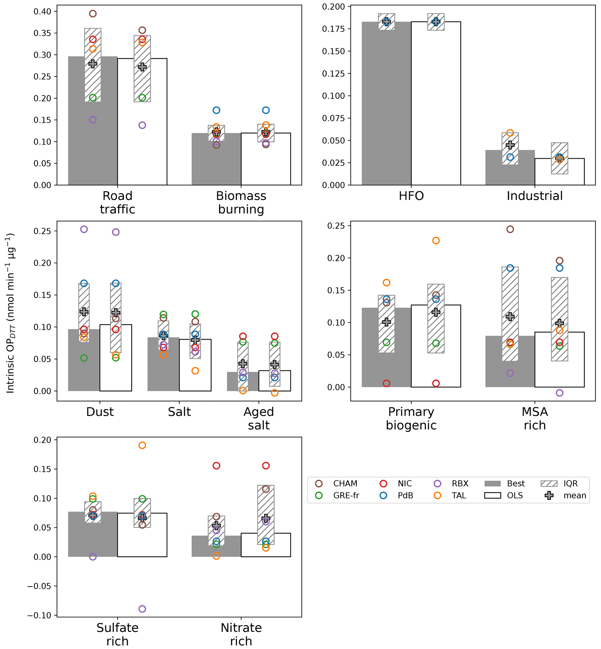
Figure 9 Intrinsic OP_DTT estimated by the best model and the reference model in the six sites. The y axis represents the intrinsic OP values in nmol min⁻¹ µg⁻¹, and the x axis represents the sources. The gray bars are the median intrinsic OP values of the best models in the six sites (n=500 bootstrapping × number of sites where the given source is detected) for each source. The white bars are the same median intrinsic OP values for the reference (OLS) model. The gray plus symbol represents the mean of intrinsic OP values. The hatched bars are the interquartile ranges of the intrinsic OP values. The dots represent the mean intrinsic OP of all sites, including gray – Chamonix, green – Grenoble, red – Nice, blue – Port-de-Bouc, purple – Roubaix, and orange – Talence.

While the best model and reference model give the same mean intrinsic OP_DTT for all sites, the mean OP_DTT at each individual site can vary substantially between the two models. The best model exhibited the positive intrinsic OP for all sources, while the reference model displayed negative intrinsic OP in RBX (MSA-rich and sulfate-rich sources). Especially in the case of sulfate-rich sources in RBX, the negative intrinsic OP in the reference model passed the threshold of the negative value, which presented a 110 % reduction compared to the mean intrinsic OP of all sites. This is also found in the OP_AA comparison, which confirmed that the best model generates a geochemical meaningful intrinsic OP. In addition, the best model exhibited consistent intrinsic OP across sites, especially for the dust, salt, primary biogenic, and sulfate-rich sources in TAL (heteroscedasticity is presented in this site), where intrinsic OP in TAL in the best model is more similar to the other sites. For instance, the reference model showed that the intrinsic OP in TAL is 0.20 nmol min⁻¹ µg⁻¹, far from the mean of all sites (0.07 nmol min⁻¹ µg⁻¹). We observed the same for the intrinsic OP of the nitrate-rich source in CHAM (where the heteroscedasticity is detected), which displayed a less dissimilar OP in CHAM compared with the other site in the best model. This again validates the conclusion in the OP_AA comparison, demonstrating that respecting the model assumption is essential for obtaining a robust OP SA result.

The comparison of intrinsic OP between the best model and the reference model highlights the importance of considering the database characteristics when selecting a model for OP SA. For all the datasets studied here, using the best model for each site delivered more robust results, with reduced uncertainty and reduced differences in intrinsic OP across sites, and it provided a more geochemically meaningful intrinsic OP. The recommendation for selecting a model based on the characteristics of the database is presented in Sect. 3.5.

3.5 Guidelines for the selection of a regression model for OP SA

Our results have highlighted the benefits of choosing a model that matches the characteristics of the data to improve the robustness of the OP SA method. For this reason, this section develops a workflow to help make model selection decisions. Before selecting a regression for OP SA, the first question is whether the PM₁₀ sources are collinear and the second is whether the residual variance of the regression between OP and PM₁₀ mass is constant. These two questions represent the characteristics of PM₁₀ sources and OP activities, which vary according to the study site.

Figure 10 Workflow in model selection considering the data characteristics.

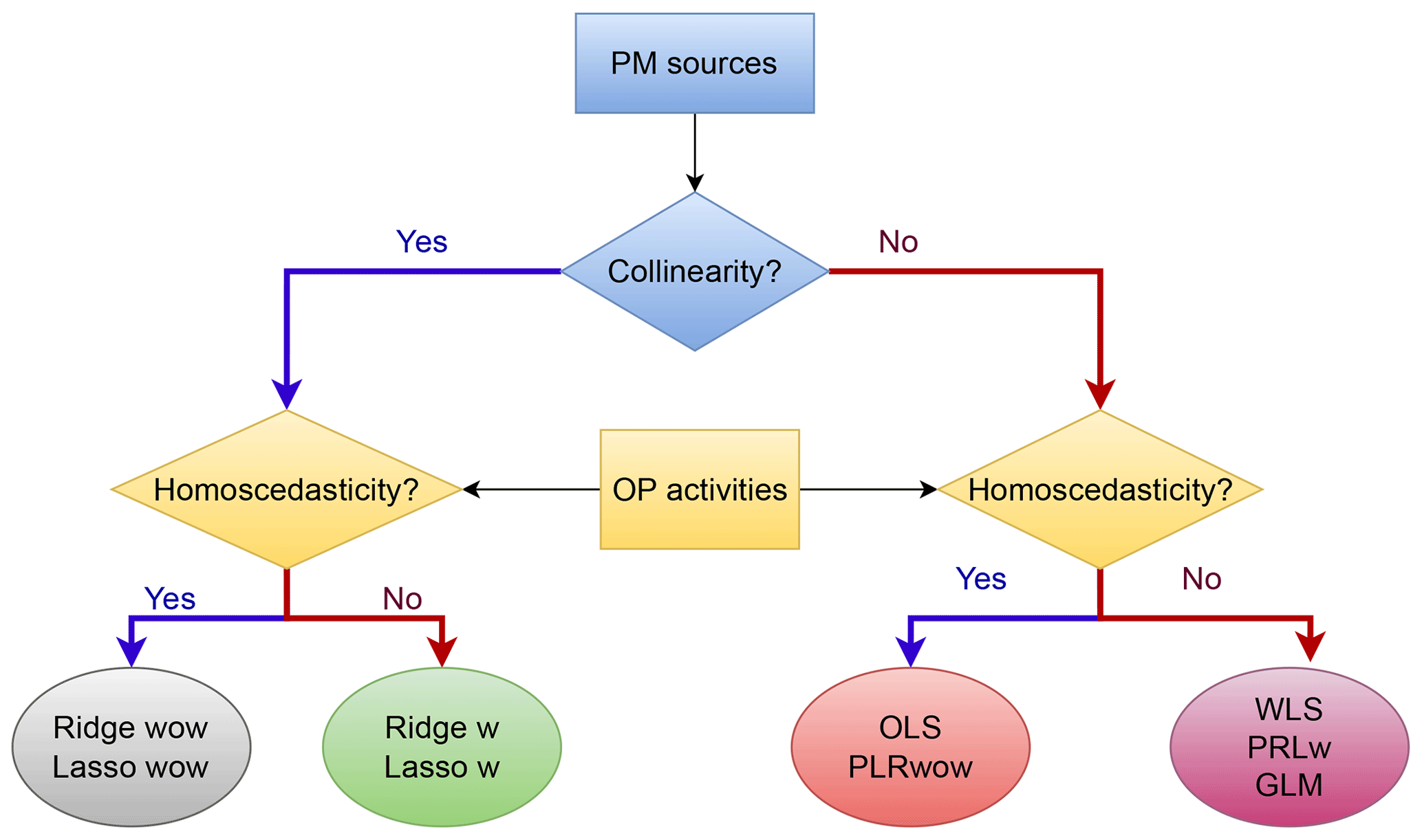
For data exhibiting collinearity between sources and generating a residual variance that varies according to the value of the PM₁₀ sources, weighted regularization regression can help to reduce collinearity and to match the model assumption about the residual. On the other hand, unweighted Ridge and Lasso are introduced for data showing collinearity and homoscedasticity. Additionally, data with no collinearity are suitable for OLS and unweighted PLS in the case of homoscedasticity, while WLS and weighted PLS are used for data with heteroscedasticity.

If the number of predictors (PM₁₀ sources) is below the number of samples divided by 15, RF and MLP can also be employed to capture possible non-linear relationships between the OP and PM₁₀ sources. However, cross-validation must be used to ensure that there is no over-fitting. In addition, these models do not estimate intrinsic OP (nmol min⁻¹ µg⁻¹) but only the importance of each PM₁₀ source to the OP prediction. This is a major drawback, since the intrinsic OP of sources is a prerequisite for the modeling effort of OP with CTM. However, RF and MLP could be useful for OP prediction in the case of larger datasets generated by online instruments.

For each data characteristic there is more than one model that is suitable. Out-of-sample performance metrics should be employed to identify the most accurate of these models.

Finally, these techniques of OP apportionment could not be performed well with uncertain PMF-derived sources. The PMF results sometimes do not adequately represent PM mass concentration for several reasons, such as the lack of a trace species to identify a source, an insufficient sample size, the source contribution being too small to be identified (under 1 %), or collinearity issues. Important information could be missed because of these problems in PMF implementation, which is explained by the model's low accuracy. Our study did not encounter this problem, since the PMF is harmonized and performed according to European recommendations which could perform the regression technique well and make it possible to obtain a very satisfactory successive OP modeled in comparison with observations after regression techniques (R² from 0.7 to 0.9). However, this problem could potentially happen, and for these cases, we could recommend either subtracting the total source contribution from the PM mass concentration to get the part that PMF cannot simulate. The information in this part may contain vital sources. Alternatively, it is possible to re-execute the PMF to validate the result and ensure the robustness of the chemical profile and the contribution of sources.

Limitations and perspectives of the study:

• This study compares eight regression models but is not exhaustive; further research could add more regression techniques to evaluate result variations across models. The potential techniques that could be applied for OP SA are gradient boosting techniques for resolving regression models or supervised machine learning techniques which enable the investigation of linear and non-linear regression relationships. However, the consistently strong performance of ordinary linear regression across six locations in France suggests that there may be little to gain from applying more complex models in areas with similar PM₁₀ sources.

• PMF coupled with a regression model remains a popular approach for OP SA. Notably, the uncertainties in PMF are typically addressed in chemical profiles but not in contributions. Incorporating uncertainty from variations in contributions into models could enhance their robustness compared with relying only on absolute PMF results.

• Observations ranged between 100 and 200 samples at each site, which may be insufficient to obtain a fair performance of GLM, decision tree, and neural network models, even though this number of samples is sufficient to address SA through the PMF model for offline analyses. Therefore, this study outlines well the limitations of GLM, RF, and MLP for offline datasets. Future investigations should be performed in an extended dataset, such as long-term or real-time measurement data, to investigate the performance of machine learning algorithms.

• This study only focused on the two most popular OP assays of PM₁₀ (OP_DTT and OP_AA). However, there are various OP assays available, such as OP_DCFH, OP_OH, OP_FOX, OP_GSH and OP_ESR, and different sizes of PM (PM₁, PM_2.5, PM₅). Further research should include more OP assays, which can be helpful in evaluating the performance of various regression models for different OP and different PM sizes.

• This study used the analytical uncertainty as the weighting for the weighted model. However, the weighting can be selected based on different ways, as reported by Montgomery et al. (2012): (1) prior information from the theoretical model, (2) using the residual extracted from the OLS model, (3) selecting the weighting based on the uncertainty of the instrument if the dependent variable is measured by a different method, and (4) selecting the weighting based on the error of these observations if the dependent variable is the average of different observations.

4 Conclusion

The results of the OP SA marked an important milestone as they were revealed for the first time through the use of eight regression models, including OLS, WLS, PLS, GLM, Ridge, Lasso, RF, and MLP. This in-depth analysis was carried out on a complete set of data collected from six sites with different characteristics. The approach of selecting a suitable model for each site based on specific data characteristics resulted in a more consistent intrinsic OP across sites, in stark contrast to the variation observed when using the basic OLS model. The revelations of the study have provided concrete recommendations for the judicious selection of an appropriate regression model based on the unique characteristics of the dataset. These guidelines should help to improve the accuracy of OP assessments and contribute to the refinement of air quality assessment methods. In addition, the implications of this research extend to the implementation of OP monitoring as a new measure of air quality, particularly on European supersites. As this initiative aligns with the ongoing revision process of European Directive 2008/50/CE, the findings of the study assume a pivotal role in shaping the methodologies underpinning air quality assessments on a broader regulatory level.