the Creative Commons Attribution 4.0 License.
the Creative Commons Attribution 4.0 License.
 | 12 Jun 2024
Diagnosing uncertainties in global biomass burning emission inventories and their impact on modeled air pollutants
Wenxuan Hua
Sijia Lou
Xin Huang
Zilin Wang
Aijun Ding
Large uncertainties persist within current biomass burning (BB) inventories, and the choice of these inventories can substantially impact model results when assessing the influence of BB aerosols on weather and climate. We evaluated discrepancies among BB emission inventories by comparing carbon monoxide (CO) and organic carbon (OC) emissions from seven major BB regions globally between 2013 and 2016. Mainstream bottom-up inventories, including the Fire INventory from NCAR 1.5 (FINN1.5) and Global Fire Emissions Database version 4s (GFED4s), along with the top-down inventories Quick Fire Emissions Dataset 2.5 (QFED2.5) and Visible Infrared Imaging Radiometer (VIIRS-)based Fire Emission Inventory version 0 (VFEI0), were selected for this study.
Global CO emissions range from 252 to 336 Tg, with regional disparities reaching up to a 6-fold difference. Dry matter is the primary contributor to the regional variation in CO emissions (50 %–80 %), with emission factors accounting for the remaining 20 %–50 %. Uncertainties in dry matter often arise from biases in calculating bottom fuel consumption and burned area, influenced by vegetation classification methods and fire detection products. In the tropics, peatlands contribute more fuel loads and higher emission factors than grasslands. At high latitudes, increased cloud fraction amplifies the discrepancy in estimated burned area (or fire radiative power) by 20 %. The global OC emissions range from 14.9 to 42.9 Tg, exhibiting higher variability than CO emissions due to the corrected emission factors in QFED2.5, with regional disparities reaching a factor of 8.7.
Additionally, we applied these BB emission inventories to the Community Atmosphere Model version 6 (CAM6) and assessed the model performance against observations. Our results suggest that the simulations based on the GFED4s agree best with the Measurements of Pollution in the Troposphere (MOPITT-)retrieved CO. While comparing the simulation with the Moderate Resolution Imaging Spectroradiometer (MODIS) and AErosol RObotic NETwork (AERONET) aerosol optical depth (AOD), our results reveal that there is no global optimal choice for BB inventories. In the high latitudes of the Northern Hemisphere, using GFED4s and QFED2.5 can better capture the AOD magnitude and diurnal variation. In equatorial Asia, GFED4s outperforms other models in representing day-to-day changes, particularly during intense burning. In Southeast Asia, we recommend using the OC emission magnitude from FINN1.5 combined with daily variability from QFED2.5. In the Southern Hemisphere, the latest VFEI0 has performed relatively well. This study has implications for reducing the uncertainties in emissions and improving BB emission inventories in further studies.
- Article
(4438 KB) - Full-text XML
-
Supplement
(2628 KB) - BibTeX
- EndNote


In recent years, extreme wildfire events have occurred frequently around the world (Balshi et al., 2009; Knorr et al., 2016; Yang et al., 2019; Junghenn Noyes et al., 2022). The size of these fires has consistently broken records over the last few decades (Westerling et al., 2006; Westerling and Bryant, 2008; Brando et al., 2020), threatened lives and infrastructure, and continuously jeopardized the global economy. Wildfires are also one of the most important sources of biomass burning (BB) emissions, which can emit loads of gaseous and particulate pollutants (Ferek et al., 1998; Adams et al., 2019) that are detrimental to regional air quality and human health (Reid et al., 2005, Reid and Mooney, 2016). Additionally, BB aerosols, predominantly black carbon (BC) and organic carbon (OC), can affect regional climate by absorbing and/or scattering solar radiation, acting as cloud condensation nuclei, and altering cloud albedo (Spracklen et al., 2011; Boucher et al., 2013). Recent studies have shown that aerosols produced by biomass burning can significantly affect changes in temperature, cloud fraction, precipitation, and even the circulation structure (Christian et al., 2019; Yang et al., 2019; Yu et al., 2019; Carter et al., 2020; Jiang et al., 2020; Ding et al., 2021; Huang et al., 2023). However, these changes in meteorology are sensitive to the choice of BB emission inventory.
Previous studies often found that there is a significant deviation between the gaseous or particulate pollutants simulated by the model and the satellite retrieval value (Bian et al., 2007; Chen et al., 2009; Carter et al., 2020); one of the most important reasons comes from the uncertainties in emission inventories. For example, Bian et al. (2007) applied six different BB emission inventories, the Global Fire Emissions Database versions 1 and 2 (GFED1 and GFED2), Arellano1, Arellano2, Duncan1, and Duncan2, to the Unified Chemistry Transport Model (UCTM). They reported that although the total global CO of the six BB emission inventories was within 30 % of each other, the model results suggested that regional deviations can be much higher by 2–5 times, especially in the Southern Hemisphere. Therefore, bias in emission inventories can often significantly impact the direct and indirect effects of models on aerosol assessments (Liu et al., 2018; Ramnarine et al., 2019; Carter et al., 2020; L. Liu et al., 2020). Carter et al. (2020) compared simulated black carbon (BC) and organic carbon (OC) concentrations with measurements from the Interagency Monitoring of Protected Visual Environments (IMPROVE) observation network from May to September. They suggested that using the Fire INventory from NCAR 1.5 (FINN1.5) inventory improves model results in eastern North America, while using the GFED4s, the Quick Fire Emissions Dataset 2.4 (QFED2.4), and the Global Fire Assimilation System 1.2 (GFAS1.2) inventories shows better agreement with observations in western North America. They also noted that population-weighted BB PM2.5 concentrations in Canada and the adjacent United States could vary between 0.5 and 1.6 µg m−3 in 2012 by using different BB emissions. Liu et al. (2018) used the global Community Atmosphere Model 5 (CAM5) and three different BB emission inventories to analyze the uncertainties in the aerosol radiative effects in the northeastern United States in early April 2009. They found that aerosols exhibited a stronger cooling effect when CAM5 used the QFED2.4 inventory rather than the GFED3.1 and GFED4s inventories, with additional cooling of −0.7 and −1.2 W m−2 through the aerosol direct radiative effect and the aerosol–cloud radiative effect, respectively. On a global basis, Ramnarine et al. (2019) used the GEOS-Chem-TwO-Moment Aerosol Sectional (GEOS-Chem-TOMAS) global model and found that the direct radiative effects and indirect effects of aerosols driven by the FINN1.5 emission inventory in 2010 were 70 % and 10 % lower than those driven by GFED4, respectively. Therefore, to better estimate regional aerosol–radiation/aerosol–cloud interactions in wildfire regions, it is necessary to understand the differences in emission inventories from biomass combustion and the main drivers of uncertainties.
In general, BB emission inventories are based on bottom-up or top-down methods to infer the emission source intensity. The bottom-up approach, also known as the fire detection and/or burned area method, estimates emissions based on surface data such as fuel loading, active fire counts, and/or burned area. Currently, the widely used BB inventories based on the bottom-up approach include Duncan (Duncan et al., 2003), GFED (van der Werf et al., 2006, 2010, 2017), FINN (Wiedinmyer et al., 2011), and the Global Inventory for Chemistry-Climate Studies-GFED4S (G-G) (Mieville et al., 2010). The top-down approach uses satellite observations of fire radiative power (FPR), a method to measure the radiative energy release rate of burning vegetation, to estimate emissions by fuel consumption. The BB inventories based on the top-down method include Arellano (Arellano et al., 2004; Arellano and Hess, 2006), GFAS (Kaiser et al., 2012), Fire Energetics and Emission Research (FEER) (Ichoku and Ellison, 2014), QFED (Darmenov et al., 2015), the Fire Emissions Estimate Via Aerosol Optical Depth (FEEV-AOD) (Paton-Walsh et al., 2012), and the recently released Visible Infrared Imaging Radiometer (VIIRS-)based Fire Emission Inventory version 0 (VFEI0) (Ferrada et al., 2022). On a global scale, the average annual BB emissions of CO and OC can differ by a factor of 3 to 4, with the global emissions fluctuating in the range of 280–580 and 13–50 Tg yr−1, respectively. The bias may be even greater when focusing on emissions in specific regions (Bian et al., 2007; Liousse et al., 2010; Williams et al., 2012; Carter et al., 2020; Lin et al., 2020b; T. Liu et al., 2020). For example, the estimated CO emission of the Arellano inventory in South America during the burning peak season of September 2000 is 4 times greater than that of the GFED1 inventory (Bian et al., 2007). A recent study has even found that since 2008, OC emissions from QFED2.5 in the Middle East have been approximately 50 times larger than those from GFED3 and GFED4 (Pan et al., 2020).
Several previous studies have analyzed the reason for the huge emission bias. According to Darmenov et al. (2015), the emissions Ei (mass of pollutant i) is the sum of the products of the emission factor (EF) and the dry matter (DM) for each biome. While earlier studies suggested that the uncertainty in BB emissions arises mainly from differences in emission factors (e.g., Alvarado et al., 2010; Akagi et al., 2011; Urbanski et al., 2011), more recent studies point out that uncertainty in dry matter also plays an important role (Paton-Walsh et al., 2010, 2012; Carter et al., 2020). For example, Paton-Walsh et al. (2012) assessed the difference in CO emissions from the February 2009 Australian fire and found that total CO emissions in GFED3.1 were roughly 3 times higher than those in FINN1, with DM contributing up to 80 %. Carter et al. (2020) evaluated emissions from various North American BB inventories over the 2004–2016 period and found that changes in DM were very close to the emission trend, suggesting that uncertainty in potential DM rather than EF across North America was the primary factor.
The accuracy of BB inventories is influenced by land cover and land use (LULC) data, impacting both EFs and DM (Wiedinmyer et al., 2006; Ferrada et al., 2022). In a study by Wiedinmyer et al. (2006), three distinct LULC products were employed to drive a regional BB emissions model. The variations in LULC products led to discrepancies in fuel consumption, resulting in an annual bias of up to 26 % in North and central America. Moreover, EFs are closely tied to different biomes, introducing uncertainty into BB emission inventories with varied biome classifications (Ferrada et al., 2022). In addition to LULC products, uncertainties are introduced by fire detection products (such as FRP and burned area products), affected by factors such as satellite transit time and cloud obscuration. For example, Paton-Walsh et al. (2012) found that in an Australian fire called Black Friday in February 2009, the burned areas of FINN1 were barely half of those of GFED3.1. T. Liu et al. (2020) reported that compared with the active fire area used in FINN1.5, the burned area product selected by GFED4s is less sensitive to the satellite overpass time and cloud obscuration. These results indicate that LULC and fire detection products are key factors leading to bias in BB emission estimation.
Although previous work has generated biomass burning emission inventories and attempted to reduce their uncertainties (Duncan et al., 2003; Arellano et al., 2004; Arellano and Hess, 2006; van der Werf et al., 2006, 2010, 2017; Bian et al., 2007; Mieville et al., 2010; Wiedingmyer et al., 2011; Kaiser et al., 2012; Paton-Walsh et al., 2012; Ichoku and Ellison, 2014; Darmenov et al., 2015; Liu et al., 2018; Ramnarine et al., 2019; Carter et al., 2020; Lin et al., 2020b; T. Liu et al., 2020; Pan et al., 2020; Zhang et al., 2020; Ferrada et al., 2022), they did not analyze the reasons why DM and EF exhibited large differences among various emission inventories, which may vary over time and location. Here, this study aims to explore the underlying reasons for the differences in BB emission inventories in major combustion regions around the world, thereby attempting to reduce the uncertainties of the impact of BB emission inventories on model results. To minimize the interference of anthropogenic emissions on model results, we selected combustion regions satisfying the following conditions: (1) regional BB CO emissions are above 20 Tg yr−1; (2) BB CO emissions contribute more than 70 % of the total. We ultimately selected seven major burning areas as shown in Fig. 1, including boreal North America (BONA), southern hemispheric South America (SHSA), northern hemispheric Africa (NHAF), southern hemispheric Africa (SHAF), boreal Asia (BOAS), Southeast Asia and India (SEAS), and equatorial Asia (EQAS).
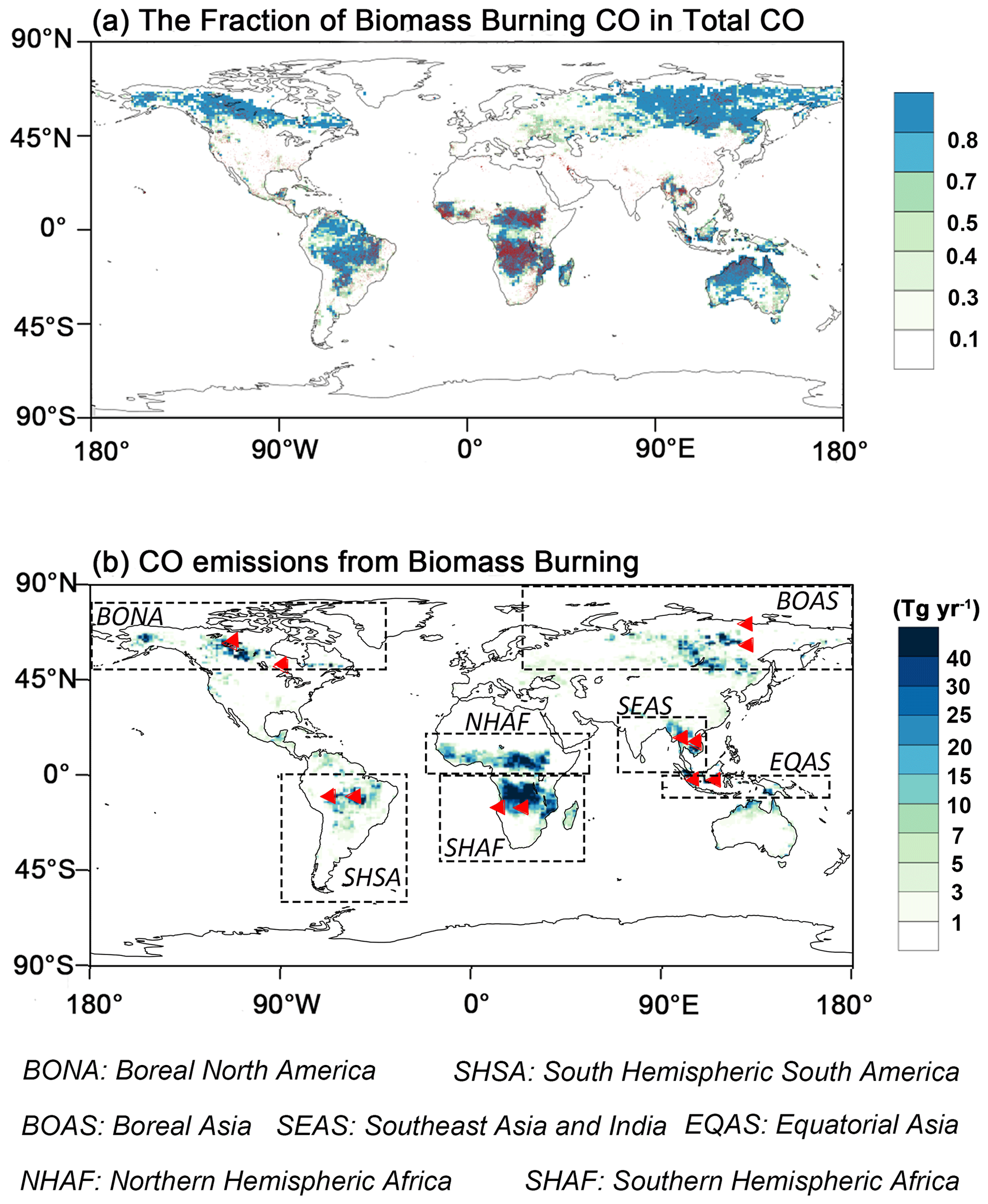
Figure 1(a) The fraction of BB CO emissions to the sum of anthropogenic and BB CO emissions (CO_BB/CO_Total) during 2013–2016 and (b) the spatial distribution of CO emissions (FINN1.5 was used as an example). The red dots in (a) are the fire points from the MCD14DL satellite product. In (b), seven regions with high BB emissions taken from those applied by van der Werf et al. (2006, 2010) are marked with black boxes, and the red triangles represent 12 AERONET stations. In this study, the seven major BB regions include boreal North America (BONA), boreal Asia (BOAS), Southeast Asia (SEAS), equatorial Asia (EQAS), Northern Hemisphere Africa (NHAF), Southern Hemisphere Africa (SHAF), and Southern Hemisphere South America (SHSA).
In this study, we compare several widely used datasets (FINN1.5, GFED4s, and QFED2.5) and the recently released VFEI0. The former two datasets are based on the bottom-up method, while the latter two are based on the top-down method. Specific details of these BB inventories are described in Sect. 2. In Sect. 3, we explore the differences in CO and OC emissions among the four inventories, examining the contributions of DM and EFs to these differences, respectively. For the first time, we evaluate the biases in CO column concentrations and AOD driven by BB inventories in the Community Earth System Model version 2.1 (CESM2)-CAM6 model. Based on our findings, we provide recommendations on which inventory should be adopted across various regions. Section 4 presents the conclusion and discussion, and our research is expected to offer insights into reducing the uncertainties with BB emission datasets.
2.1 Biomass burning emission inventories
We simultaneously diagnosed the differences between two bottom-up approach inventories and two top-down approach inventories, including FINN1.5, GFED4s, and QFED2.5, which are commonly used in the current atmospheric model, as well as the recently released VFEI0. Details about the emission inventories and the satellite products they use are listed in Table 1 and Text S1 in the Supplement.
Table 1Brief introduction to the four BB inventories.
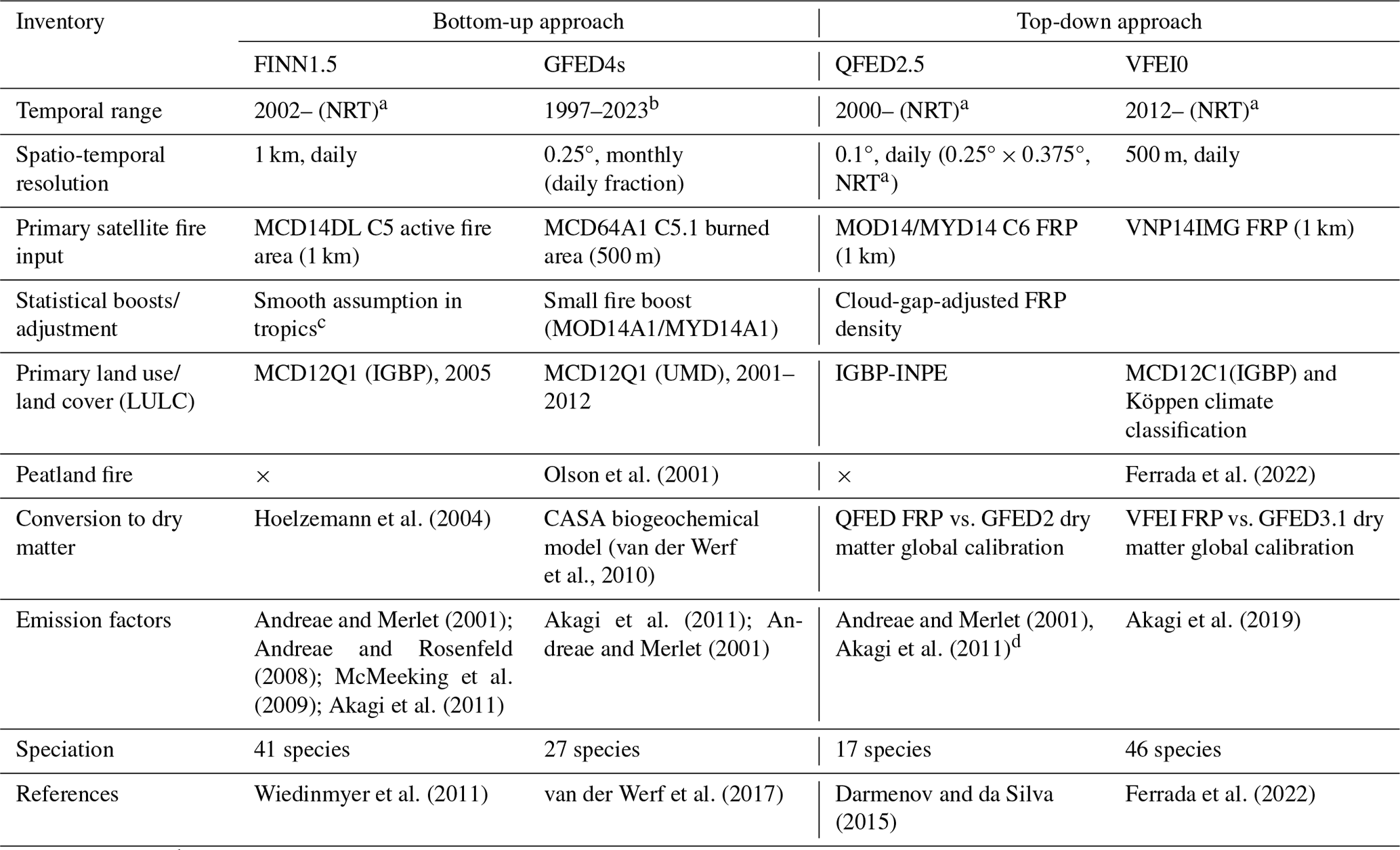
a NRT – near real time. b 2017–2022 are beta version releases. c In the equatorial region (30° N–30° S), each detected fire will be counted as 2 d, assuming the second day's fire will continue to be half the size of the previous day's. d Particulate-matter-related emissions from biomass burning (e.g., BC, OC, NH3, SO2, and PM2.5) were corrected from emission factors based on MODIS AOD.
2.1.1 Bottom-up (burned area) inventories
In this study, both FINN1.5 and GFED4s adopt a bottom-up approach (also called the burned area method), and the details are shown in Table 1. FINN1.5 uses the Moderate Resolution Imaging Spectroradiometer (MODIS) product MCD14DL for burned area calculations. This active fire detection product monitors real-time fire points larger than 0.05 km2. However, it is important to note that if a fire occurs when the satellite is not in transit or is obscured by clouds during transit, it will not be detected (Firms, 2017). Additionally, FINN1.5 assumes that every fire detected at the Equator (30° N–30° S) will persist the next day at half the size of the previous day's fire (Table 1). However, this assumption may not accurately reflect real-world conditions (Wiedinmyer et al., 2011; Pan et al., 2020). The land cover classification in FINN1.5 is based on MCD12Q1 (IGBP, version 2005). According to the IGBP land cover classification, each fire is initially assigned to 1 of 16 land use/land cover (LULC) classes and then lumped into 6 generic categories, including tropical forest, temperate forest, boreal forest, savanna and grasslands, woody savannas and shrublands, and cropland (Table S1 in the Supplement, Wiedingmyer et al., 2011). Emission factors (EFs) for various gaseous and particulate species are determined from a dataset compiled by Akagi et al. (2011) and Andreae and Merlet (2001), with these EFs varying for different LULC types. Currently, FINN1.5 has been providing daily global emissions from biomass burning since 2002, including 41 species, with a spatial resolution of 1 km2 (Table 1).
GFED4s differs in that it primarily uses the MCD64A1 Collection 5.1 burned area product (Giglio et al., 2013; Randerson et al., 2018), capable of detecting fires larger than 500 m×500 m. For small fire areas, GFED4s incorporates active fire detection products (MOD14A1 and MYD14A1), compensating to some extent for the lower spatial resolution of the original product MCD64A1 (van der Werf et al., 2017). In general, burned area products reduce uncertainty in fire detection due to satellite non-transit and cloud/smoke obscuration when a burn occurs by identifying day-to-day surface variations, such as charcoal and ash deposition, vegetation migration, and changes in vegetation structure (Boschetti et al., 2019). Similar to FINN1.5, each fire in GFED4s is initially assigned to 1 of 16 LULC subcategories and then lumped into 6 categories, with the inclusion of an additional biome, peatland (Table S1). EFs for various species follow Akagi et al. (2011) and Andreae and Merlet (2001), varying across different biome categories. Currently, GFED4s has been providing daily global emissions from biomass burning since 1997, including 27 species, with a spatial resolution of 0.25°×0.25° (Table 1). However, since 2017, the DM provided by GFED4s has been derived from a linear relationship between past emissions and MODIS FRP data for the 2003–2016 period.
2.1.2 Top-down (fire radiative power) inventories
In this study, both QFED2.5 and VFEI0 use a top-down approach known as the fire radiative power (FRP) method. In contrast to the bottom-up approach, the top-down approach relies on satellite products detecting fire-radiated power rather than fire point detection. QFED2.5 uses MODIS Collection 6 MOD14/MYD14 level 2 products to estimate fire radiative power and pinpoint fire locations using MOD03/MYD03 (Darmenov et al., 2015; T. Liu et al., 2020). The FRPs are integrated over time to obtain fire radiative energy (FRE), which is converted to DM using an empirical coefficient α. The initial α values are obtained from Kaiser et al. (2009) and are adjusted monthly based on global emissions of GFED2 in 2003–2007. QFED2.5 classifies land cover using the International Geosphere-Biosphere Programme (IGBP-INPE) dataset, aggregating 17 land cover classes into 4 broad vegetation types (Table S1, Darmenov and da Silva, 2015). Initially, EFs for various species in QFED2.5 also follow Akagi et al. (2011) and Andreae and Merlet (2001). But for certain species, including organic carbon (OC), black carbon (BC), ammonia (NH3), sulfur dioxide (SO2), and particulate matter with a diameter < 2.5 µm (PM2.5), QFED2.5 incorporates a scaling factor to enhance the EFs. QFED2.5 has been providing daily global BB emissions since 2000, including 17 species, with a spatial resolution of 0.1°×0.1° (Table 1).
VFEI0 also adopts the top-down method but uses the VNP14IMG.001 FRP product from the Visible Infrared Imaging Radiometer (VIIRS) I-band. This product has a higher resolution (375 m at nadir) compared to MODIS (1 km resolution at nadir), enabling the detection of smaller and colder flames (Ferrada et al., 2022). VFEI0 uses an empirical coefficient α derived from the linear regression of GFED3.1 DM and VIIRS FRP to convert detected FRE into DM. VFEI0 uses MCD12C1 (IGBP, version 2015) as the underlying LULC data, supplemented by Köppen climate classification (Beck et al., 2018), defining 10 subcategories in VFEI0 (Table S1). VFEI0 groups these subcategories into six biomes, corresponding to EFs provided by Andreae (2019). Currently, VFEI0 has been offering daily BB emissions since 20 January 2012, covering 46 emitted species with a horizontal resolution of 0.005°×0.005° (Table 1).
2.2 The calculation of EFs and DM
To calculate regional EFs and DM, we adopt the approach outlined by Carter et al. (2020). Initially, we divide CO emissions per grid by the EF applied to each biome, yielding DM:
where b represents one of the seven biomes in Table S1, and x represents the location grid. This calculation of DM using CO is reasonably representative, given that the inventories are not adjusted for CO emission factors. After calculating DMb,x for each grid, we derive a regional average emission factor by dividing total CO emissions by total DM for each major BB region:
These calculations enable us to discern the influence of LULC classification on BB emission inventories. For a specific biome type within a given region, we calculate EF by dividing the CO emissions of that particular biome classification by the sum of the value from each biome in the respective region:
where b represents one of the seven biome classifications in this study (Table S1).
Furthermore, for the two bottom-up inventories, we invert the fuel consumption for each vegetation biome b within a given area:
Here, the DM corresponding to each biome in FINN1.5 and GFED4s is obtained using Eq. (1), and BA represents the total burned area derived from the emission inventory.
2.3 Quantitative statistical methods
As described in Sect. 2.1, fire detection is greatly affected by cloud/smoke obscuration in the bottom-up approach. For example, if there are clouds/smoke at high altitudes while fire occurs on the ground, the MCD14DL active fire detection product used in FINN1.5 may miss these fire points. In addition, the combustion that is too small in size and too low in temperature cannot be effectively monitored due to the low brightness temperature contrast with the surrounding environment. In contrast, the burned area product (mainly MCD64A1) used by GFED4s determines the burning information based on the changes such as surface albedo and is, therefore, less affected by clouds/smoke. For inventories based on the top-down approach, the emission inventories also differ to a large extent due to the cloud/smoke obscuration, since QFED2.5 uses a “sequential method” to correct for missing FRPs during cloud/smoke obscuration, whereas VFEI0 does not. Thus, in this study, the symmetrical mean absolute percentage error (SMAPE) and Pearson's R are used to assess the difference in sensitivity to clouds/smoke between the two BB products based on the bottom-up (or top-down) approach. The specific algorithm is as follows:
where X and Y are fire detection data from two different datasets (e.g., burned area from FINN1.5 and GFED4s or FRP from VFEI0 and QFED2.5). We divided these fire detection data into three groups according to the cloud fractions less than 0.4, 0.4–0.7, and greater than 0.7, and the number n represents valid samples in different cloud fraction groups. SMAPE ranges from 0 % to 200 %, with smaller values indicating smaller differences, while Pearson's R ranges from 0 to 1, with smaller values implying less correlation.
In order to quantify the effect of cloud obscuration on BB datasets, we selected the most intensely burning regions in BONA in July for this study. For consistency, we re-interpolated the fire detection data used in the four BB datasets, as well as the MODIS MCD06 cloud fraction data, to the same horizontal resolution (0.25°×0.25°). Considering the continuity of combustion, we took every 5°×5° as a sample area in the northern US to ensure that if a large burn occurred, the area would be detected to some extent, avoiding errors due to differences between the inventories. At the same time, we excluded the samples in the same time and location, where the emissions are all zero. Finally, a total of 1888 samples were obtained for the burned area group, with 534, 541, and 813 samples for low (< 0.4), medium (0.4–0.7), and high (> 0.7) cloud fraction, respectively. A total of 1682 samples were obtained for the FRP group, with 860, 390, and 432 samples under low, medium, and high cloud fraction, respectively. It is worth noting that we use the average FRP of MOD and MYD for QFED2.5 since the VFEI0 FRP is the average between day- and nighttime observations. Moreover, our approach cannot rule out the case of missing measurements when two sets of BB inventories are both obscured by the cloud. However, the main goal of this paper is to explore the causes of uncertainties in emission inventories; the specific case of omission due to cloud obscuration depends on the development of satellite detection technology and is not part of the purpose of this study.
2.4 CESM2-CAM6 model
The Community Earth System Model version 2.1 (CESM2) is a new generation of the coupled climate–Earth system models developed by the National Center for Atmospheric Research (NCAR). In this study, we used the global Community Atmosphere Model version 6 (CAM6) (Danabasoglu et al., 2020). Gas-phase chemistry was represented by the Model for Ozone and Related chemical Tracers tropospheric chemistry (MOZART-T1; Emmons et al., 2020). The wet deposition of soluble gaseous compounds in CAM6-Chem is based on the scheme of Neu and Prather (2012), which describes the process of in-cloud cleaning and under-cloud cleaning. The formation of secondary organic aerosols (SOAs) is from a volatility basis set (VBS) approach developed by Tilmes et al. (2019). Properties and processes of aerosol species of black carbon (BC), primary organic aerosols (POAs), SOAs, sulfate, dust, and sea salt are calculated by the Modal Aerosol Module (MAM4) described by Liu et al. (2016). CAM6 uses a horizontal resolution of nominal 1° (1.25°×0.9°, longitude by latitude) and 32 vertical levels from the surface to 2.26 hPa (∼ 40 km).
In this study, four BB emission inventories (FINN1.5, GFED4s, QFED2.5, and VFEI0) are regridded to a horizontal resolution of 1.25° (longitude) × 0.9° (latitude) and then applied to the model. All simulations are performed for 5 years, while horizontal winds and temperature are nudged toward the Modern-Era Retrospective analysis for Research and Applications version 2 (MERRA-2) reanalysis data (GMAO, 2015) every 6 h. Simulations are conducted for 2012–2016, with the first year used for initialization and model spin-up. Daily BB emissions are applied in this study, whereas the vertical distribution of fire emissions is followed Freitas et al. (2006, 2010). Anthropogenic and biogenic emissions in this study are from the Community Emissions Data System (CEDS) and the Model of Emissions of Gases and Aerosols from Nature version 2.1 (MEGANv2.1), respectively, at 2010 levels (Guenther et al., 2012; Hoesly et al., 2018).
2.5 Measurement data
The Measurements of Pollution in the Troposphere (MOPITT) is aboard the Earth Observing System (EOS)/Terra satellite launched by NASA (Warner et al., 2001). MOPITT is the first instrument to observe the global concentration and has been providing the column concentration and volume mixing ratio of global carbon monoxide (CO) since 1999. We used MOPITT CO gridded monthly means (near- and thermal infrared radiances) V009 (MOP03JM_9; NASA Langley Atmospheric Science Data Center DAAC, retrieved from https://doi.org/10.5067/TERRA/MOPITT/MOP03JM.009, NASA/LARC/SD/ASDC, 2024), which has a horizontal resolution of 1°×1°. It should be noted that to compare the CO column concentration simulated by CESM2-CAM6 with MOPITT CO, we calculated the simulated CO column concentrations by cumulative integration from 900 to 100 hPa isobaric height (Deeter et al., 2022). We also used the daily AOD (550 nm) and cloud fraction data from the MODIS products MOD08_D3 (MODIS/Terra Aerosol Cloud Water Vapor Ozone Daily L3; Platnick et al., 2015) and MCD06COSP (MODIS (Aqua/Terra) Cloud Properties level 3 daily, Webb et al., 2017), respectively.
The observations of AERONET (http://AERONET.gsfc.nasa.gov/, last access: 11 February 2023; Holben et al., 1998) from 12 sites are used in this study. These AERONET stations were selected since they are close to BB source regions. As marked in Fig. 1b, these sites include sites in BONA (Yellowknife, Aurora (62.5° N, 114.4° W), Pickle Lake (51.4° N, 90.2° W)), BOAS (Tiksi (71.6° N, 128.9° E), Yakutsk (61.7° N, 129.4° E)), SHAF (Namibe (15.2° S, 12.2° E), Mongu Inn (15.3° S, 23.1° E)), SHSA (Alta Floresta (9.9° S, 56.1° W), Rio Branco (9.9° S, 67.9° W)), EQAS (Palangkaraya (2.2° S, 113.9° E), Jambi (1.6° S, 103.6° E)), SEAS (Omkoi (17.8° N, 98.4° E), Ubon Ratchathani (15.2° N, 104.9° E)).
Each observed AOD represents real atmospheric conditions, and therefore, in addition to BB aerosols, biogenic aerosols, anthropogenic aerosols, dust, and sea salts are also integrated in MODIS and AERONET datasets.
CO and OC are the main species emitted from biomass burning (van der Werf et al., 2010; Carter et al., 2020), but emissions vary widely. In this study, we compare the differences in CO and OC emissions (representing gaseous and particulate pollutants, respectively) in four BB inventories and investigate in detail the key reasons for the differences in emission inventories.
3.1 The contribution of dry matter and emission factors to the difference in CO emission
The total global CO emissions from the four BB emission inventories selected for this study are in the range of 252–336 Tg, with GFED4s being the highest and FINN1.5 the lowest. To quantify the differences in CO emissions among the four datasets, we use the standard deviation (SD) to characterize the absolute difference and the coefficient of variation (cv; calculated as the ratio of SD to the mean) to characterize the relative differences (Fig. 2a). The larger the cv, the greater the difference between emission inventories. We have ranked the seven major BB regions in the world according to the differences in CO emissions between the four sets of inventories, with the differences being, in descending order, EQAS, BONA, SEAS, SHAF, NHAF, BOAS, and SHSA.
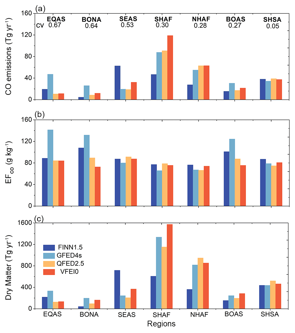
Figure 2(a) Average annual CO emissions of the four biomass burning emission inventories across seven major BB regions during 2013–2016. The cv, defined as the ratio of the standard deviation to the mean, is the coefficient of variation among the emissions of the four datasets. Panels (b) and (c) are the same as (a) but for the emission factor of CO (EFCO) and dry matter.
This study points to a high variability of different BB emission inventories in EQAS, which is inconsistent with previous studies (T. Liu et al., 2020; Pan et al., 2020). Previous studies mainly focused on emission differences of particulate pollutants, such as BC and OC (Bian et al., 2007; Paton-Walsh et al., 2012; Carter et al., 2020; Lin et al., 2020b; Pan et al., 2020), thus assuming that the inventory differences in equatorial Asia are smaller than those in southern hemispheric Africa and northern hemispheric Africa. In contrast, this study analyzes the differences between particulate and gaseous pollutant emissions separately when comparing the differences in BB emission inventories. For example, GFED4s classifies a large portion of EQAS land cover as peatland (Kasischke and Bruhwiler, 2002; Stockwell et al., 2016; van der Werf et al., 2006, 2010, 2017) and suggests that this organic-matter-rich soil emits a large amount of CO when burned. The other three inventories either do not include peatland (FINN1.5 and QFED2.5) or only consider peatlands to be a small fraction of the burned area in EQAS (VFEI0), thus estimating CO emissions much smaller than GFED4s. In addition, the extent of peatland fires in EQAS increased significantly during the strong El Niño event (Page et al., 2002). Considering that a strong El Niño event also occurred in 2015–2016, these increases in peatland fires further amplify the discrepancy between GFED4s and other emission inventories on CO estimates.
As shown in Fig. 2, the distribution pattern of DM differences is very similar to that of CO emission differences, indicating that DM is the main reason for dominating the difference in the four emission inventories. In comparison, the difference in DM contributes 50 %–80 % to the regional CO emission differences, and the comprehensive EFs contribute the remaining 20 %–50 %. However, in EQAS, BONA, and BOAS, the contribution of comprehensive EFs to BB emission differences in the four datasets is comparable to that of DM (Fig. 2). In the following sections, we further analyze the main causes of the differences in DM and EFs.
3.2 Primary causes of DM inconsistency in the bottom-up inventories
To investigate the underlying causes of the differences in DM, we first compared DM between emission inventories produced by the bottom-up and up-down approaches. The difference in DM estimated by the top-down method is small, and the DM ratio of QFED2.5 to VFEI0 does not exceed 2 in different regions. However, DM estimated by the bottom-up approach varied widely, with the DM ratio as high as 4.7 in BONA for GFED4s and FINN1.5 during the 2013–2016 fire season. Therefore, we need to focus on the main reasons for DM variance in emission inventories based on the bottom-up approach.
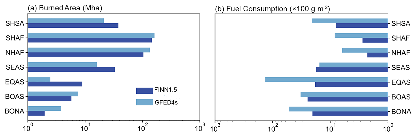
Figure 3Annual burned area (a) and fuel consumption (b) of two bottom-up datasets (FINN1.5 and GFED4s) across seven regions from 2013 to 2016.
According to Eq. (2), DM equals the product of the burned area, fuel load, and FB in the bottom-up inventories, with the product of the last two terms being fuel consumption. Figure 3 compares the burned area and fuel consumption of GFED4s and FINN1.5 emission inventories for the seven largest BB regions. The GFED4sFINN1.5 ratio represents the relative difference in burned area or fuel consumption between the two emission inventories. In general, the difference in burned area between the two inventories varies greatly with latitude, and the ratio of GFED4s to FINN1.5 fluctuates in the range of 0.28–1.94. In contrast, differences in fuel consumption between the two inventories were more consistent, with GFED4s consistently having higher fuel consumption than FINN1.5 in all regions except SEAS. In the next sections, we discuss the main reasons for the differences in burned area and fuel consumption between the two datasets.
3.2.1 Effect of land cover on burned area
As shown in Fig. 3a, the differences in the burned area between the bottom-up emission inventories are highly variable. At high latitudes, the burned area of GFED4s is significantly higher than that of FINN1.5, especially in BONA, where the burned area of GFED4s is twice that of FINN1.5. In contrast, the burned area of GFED4s in the equatorial region is much lower than that of FINN1.5 and even 60 % smaller in EQAS. This is a result of the difference in fire detection between the two datasets. As shown in Table 1, FINN1.5 uses the MCD14 DL fire point product, while GFED4s uses the hybrid burned area product, mainly using MCD64A1 combined with the fire point products MOD14A1/MYD14A1 to enhance the detection of small fires.
These two sets of products have their advantages in detection ability under different vegetation type conditions. The hybrid burned area product detects burned areas over a period of time (up to days), while the fire point product detects burned areas primarily in near real time (Roy et al., 2008). In addition, the burned area used in GFED4s (hybrid burned area product) is not affected by the vegetation canopy when the leaf area index (LAI) is less than 5. Therefore, a higher burned area is estimated in GFED4s in BONA and BOAS than in FINN1.5. However, in areas with more broadleaf forests and grasslands, such as EQAS, SEAS, and SHSA (Fig. S1 in the Supplement), the MCD14DL fire point product used in FINN1.5 performed better in capturing understory fires that occurred in closed canopies (Cochrane and Laurance, 2002; Cochrane, 2003; Alencar et al., 2005; Roy et al., 2008). It also has an advantage in capturing sporadic and fragmented small fires in grasslands and agricultural fields due to its high resolution (T. Liu et al., 2020). Furthermore, FINN1.5 assumes that each detected fire in the equatorial region will continue to burn for 2 d and that the next day's fire will continue to be half the size of the previous day's (Table 1). Thus, the burned area of FINN1.5 in the tropical zone is 2.6 times higher than that of GFED4s, which is consistent with previous studies (Wiedinmyer et al., 2011; Pan et al., 2020). At the Equator, the burned area in grassland/agricultural fields and forests estimated by FINN1.5 is 1–3 and 4–6 times higher than in GFED4s, respectively (not shown).
It is worth noting that in Africa (NHAF and SHAF), although the dominant burnable vegetation is grassland (Fig. S1), unlike the sporadic small fires that occur in grassland in the other five regions, large continuous fires often occur in African savannas (T. Liu et al., 2020). Therefore, the hybrid burned area product used in GFED4s is more effective in detecting all fire events occurring over time, with 10 %–20 % higher burned area than FINN1.5.
3.2.2 Effect of cloud obscuration on burned area
In addition to the vegetation, cloud occlusion can likewise bias the satellite detection of burned area. Figure S2 in the Supplement shows the time series of AOD measured by satellite or ground-based data at the Pickle Lack site of BONA from June to August 2013. In contrast to the high AOD values observed for the AERONET network, MODIS AOD often in missing measurements when the MODIS cloud fraction is larger than 0.5 thus may lead to a low value. Furthermore, AERONET AOD varies dramatically over a short period, suggesting that different detection principles (such as detecting fire points in near real time during satellite overpass time or estimating the accumulation of burned area over time through changes in surface albedo over multiple satellite overpass times) can significantly affect the burned area product under high-cloud-fraction/high-smoke conditions (Paton-Walsh et al., 2012; T. Liu et al., 2020; Pan et al., 2020). Although some assumptions are made in FINN1.5 in the equatorial regions as described above to improve the effect of cloud obscuration on burned area detection, these assumptions are not used for middle and high latitudes. GFED4s uses a hybrid burned area product and is relatively unaffected by cloud obscuration. By fusing the MCD64A1 product with the MOD14A1/MYD14A1 products with multi-temporal satellite data, GFED4s is able to determine the approximate date and extent of fires through post-fire ash deposition, vegetation migration, and land surface changes (van der Werf et al., 2017; Boschetti et al., 2015, 2019).
To quantitatively assess the impact of cloud obscuration on different emission inventory estimates, we perform analyses in areas with high cloud fraction (Fig. S3 in the Supplement) and intense biomass burning and that are unaffected by the smoothing hypothesis used in FINN1.5. We selected the regions of North America with the most intense biomass burning (Alberta and Saskatchewan, Canada; 50–70° E, 100–130° W; Fig. S4 in the Supplement) and analyzed the relationship between the burned area and cloud fraction for bottom-up inventories in July from 2013 to 2016 (Fig. S5 in the Supplement). As shown in Fig. 4, with the increase in cloud fraction, the SMAPE of the two bottom-up emission inventories increases from 150 % to 180 %, while the Pearson correlation declines from 0.85 to around 0.75. These results demonstrate that the uncertainty in the burned area for two bottom-up emission inventories increases by ∼ 20 % during high-cloud-fraction conditions compared to low-cloud-fraction conditions.
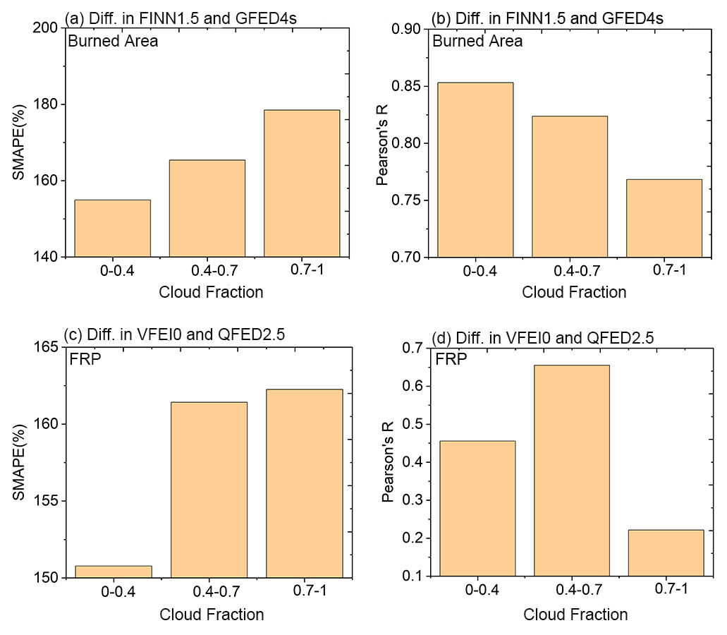
Figure 4The differences in (a, b) burned areas and (c, d) total FRP detected by two inventories under different cloud fraction conditions in a pilot region of BONA. These differences are quantified by two indicators: SMAPE and Pearson's R. Cloud fraction data are calculated from the MODIS product MCD06COSP.
3.2.3 Causes of fuel consumption differences
Fuel consumption is another factor that affects DM differences between two BB emission inventories. As shown in Fig. 3b, the fuel consumption of GFED4s is 30 %–75 % higher than that of FINN1.5 in almost all BB areas except SEAS. The difference in fuel consumption between the two emission inventories is larger in the tropics than in the high latitudes. As shown in Fig. 5, at high latitudes (e.g., BONA and BOAS) and in the equatorial region (such as EQAS), relatively high fuel consumption comes from peatlands in GFED4s. According to previous studies, peatlands, a type of soil rich in organic matter, store large amounts of carbon underground (van der Werf et al., 2010, 2017; Gibson et al., 2018; Kiely et al., 2021; Vetrita et al., 2021) and emit large amounts of CO when burned. Peatlands contribute 30 %–60 % of the total fuel consumption in BONA, BOAS, and EQAS (Fig. 5a–c).
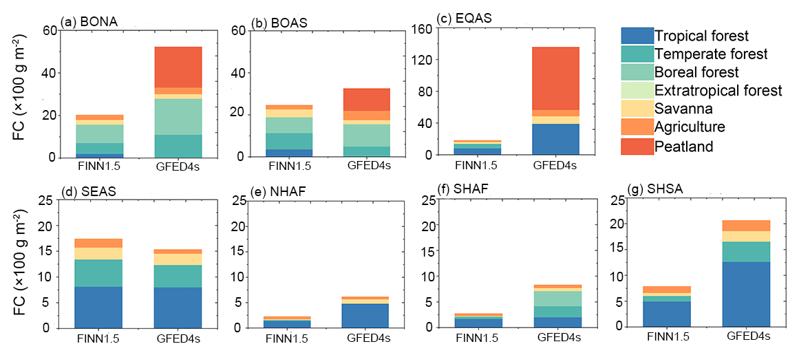
Figure 5Annual average fuel consumption of two bottom-up datasets (FINN1.5 and GFED4s) across seven regions from 2013 to 2016. The contributions of the seven biomes are shown in different colors.
Besides peatlands, GFED4s tends to have higher fuel consumption than FINN1.5 due to forest contributions. Forests (including tropical, temperate, and boreal forests) account for more than 50 % of the fuel consumption in all burning regions except EQAS, where peatlands dominate the fuel consumption. Moreover, forest fuel consumption in GFED4s is generally much higher than in FINN1.5 except in BOAS and SEAS (Fig. 5). Since fuel consumption is equal to the product of fuel load and FB (the percentage of specific plants that can be adequately burned, Eq. 2), different vegetation classifications may be responsible for large differences in fuel consumption between emission inventories. For example, for woody vegetation such as forests, GFED4s assumes a range of FB between 40 %–60 % for temperate and tropical forests and 20 %–40 % for boreal forests, while FINN1.5 assumes that all woody vegetation burns no more than 30 % (van der Werf et al., 2010; Wiedinmyer et al., 2011). Thus, in terms of FB alone, the forest fuel consumption of GFED4s is therefore 0.67–1.3 times greater than that of FINN1.5, which is one of the main reasons for the difference in fuel consumption.
3.3 Primary causes of DM inconsistency in the top-down approach
We also analyze the causes of the difference in DM between BB emission inventories estimated by the top-down method. According to Eq. (3), it is evident that the empirical factor and the radiative energy of the fire are the key factors that cause the discrepancy in the top-down emission inventories. The QFED2.5 and VFEI0 inventories we have chosen use different satellites for the fire detection products. For example, for the fire radiative power product, QFED2.5 is based on the Moderate Resolution Imaging Spectroradiometer (MODIS) inversion of the NASA Terra and Aqua combined satellites, while VFEI0 is based on the Visible Infrared Imaging Radiometer (VIIRS) inversion of the combined polar-orbiting satellites Suomi NPP and NOAA-20, although the algorithms are similar. However, there are systematic deviations due to different satellites, specific tests and metadata, and resolutions. The VIIRS 375 m fire product used by VFEI0 has a finer resolution and is more advantageous for small fire spot detection than other coarser-resolution (1 km) fire spot detection products. The FRP density used in VFEI0 is much higher than that of QFED2.5 due to the fine horizontal resolution.
The estimations of FRP and DM are strongly influenced by the horizontal resolution of satellite products. For example, in the BONA region during July (the month with the most intense burning at the position of 50–70° N, 100–130° W), the total QFED FRP (average FRP measured by MOD and MYD) is 1.5 times higher than VFEI0 (Fig. S6 in the Supplement). Additionally, the differing α values between QFED2.5 and VFEI0 in BONA can potentially result in higher DM in QFED2.5 compared to VFEI0 by a factor of 1.3–3.8. However, the actual DM in the QFED2.5 inventory is 30 % lower than in VFEI0. The relatively high FRP density used in VFEI0 (Fig. S7 in the Supplement) results in a higher DM than in QFED2.5 due to its superior horizontal resolution, enabling the precise delineation of fire areas. It is important to note that while the empirical factor also influences the amount of DM, its impact should not be as significant as the difference caused by the horizontal resolution of satellite products (Kaiser et al., 2012; Darmenov et al., 2015; Ferrada et al., 2022).
Previous studies have shown that cloud occlusion also causes bias in FRP detection (T. Liu et al., 2020). We also take BONA as a pilot region to analyze the influence of cloud fraction on FRP in QFED2.5 and VFEI0. According to Fig. 5c and d, the SMAPE of the two emission inventories rises as the cloud fraction increases, and the Pearson correlation is noticeably low under the maximum cloud fraction. While QFED2.5 uses the sequential approach (Sect. 2.1) to correct for the missing FRP in cloud-obscured fires, this correction is not considered in VFEI0. Therefore, although the two top-down emission inventories use similar algorithms, significant bias occurs under high-cloud-fraction conditions, with QFED2.5 estimating DM much higher than VFEI0.
3.4 Primary causes of EF inconsistencies
Although DM differences dominate the inconsistencies in CO emissions across major BB regions, the contribution of EFs is still not negligible in some regions. For example, in EQAS, BONA, and BOAS, the contribution of EFs is up to 50 %, which is comparable to that of DM. The comprehensive EFs of GFED4s are higher in BONA, BOAS, and EQAS regions than in other inventories, with vegetation classification being one of the most important factors (Fig. 6). For example, in EQAS at low latitudes, peatlands in GFED4s account for 65 % of the regional comprehensive EF. In contrast to GFED4s, FINN1.5 and QFED2.5 do not consider this organic-matter-rich land as a source of burning, and they classify this category of land cover type as savanna or grass. The CO emission factor for peatlands is 4 times higher than the CO emission factor for savanna or grass (Table 2), ultimately making the comprehensive EF for GFED4s 60 %–70 % higher than that of the other three datasets. It is worth noting that although the classification of peatland exists in VFEI0 (Ferrada et al., 2022) due to differences in terrestrial ecological divisions (Olson et al., 2001; https://www.worldwildlife.org/, last access: 9 June 2023), peatland identification areas are much smaller than in the GFED4s inventory. Therefore CO emissions from peatlands in GFED4s are much higher than in the VFEI0 inventory (Fig. 3-9a; Ferrada et al., 2022).
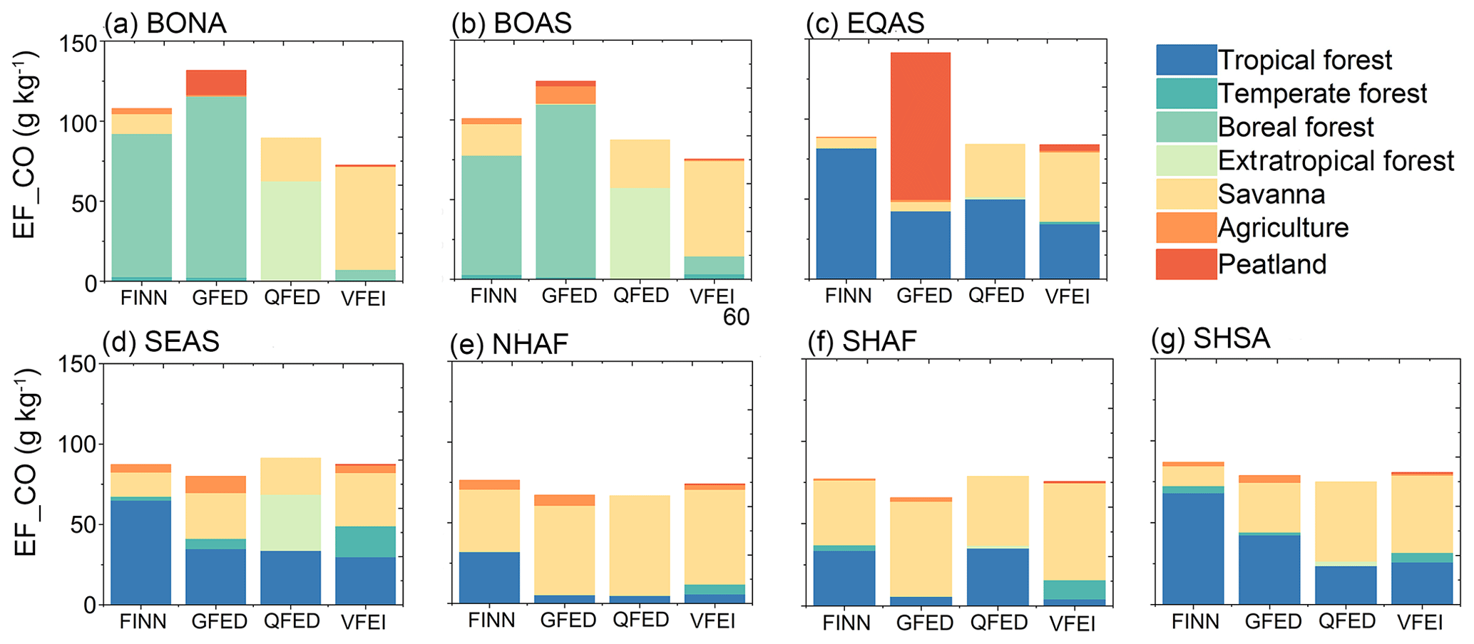
Figure 6Regional comprehensive emission factors for the four datasets (FINN1.5, GFED4s, QFED2.5, and VFEI0) in seven regions from 2013 to 2016. The contributions of the seven biomes are shown in different colors.
Table 2CO and OC emission factors used in the four biomass burning emission inventories.
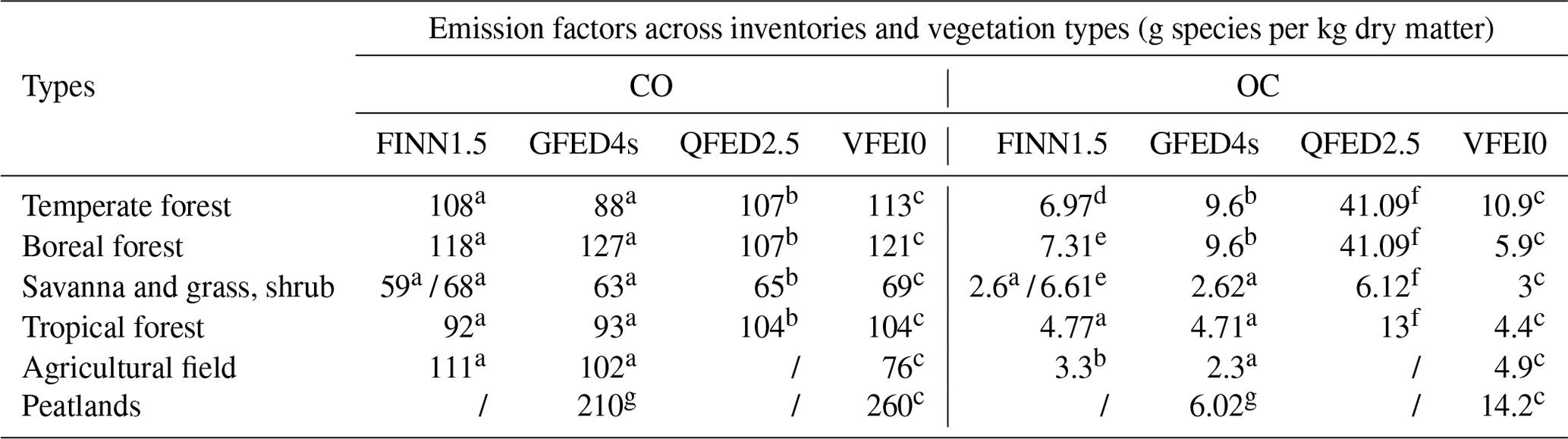
a Akagi et al. (2011). b Andreae and Merlet (2001). c Andreae (2019). d Andreae and Rosenfeld (2008). e McMeeking et al. (2009). f QFED2.5 PM-related emission factors are obtained by multiplying the base EF multiplied by its biome-specific enhancement factor. g Emission factors for peatland are the average of lab measurements of Yokelson et al. (1997) and Christian et al. (2003).
In both BONA and BOAS, we find that the comprehensive EFs in the four datasets are ranked as follows: , where the EF of GFED4s is about 1.5 times higher than that of VFEI0. Unlike the low-latitude regions, the classification of forests in different emission inventories is the main reason for the difference in comprehensive EF in high-latitude regions. At high latitudes (50–70° N), GFED4s, QFED2.5, and FINN1.5 identify more forests than VFEI0 (Table S1) because the former three classify some shrubs (e.g., closed shrublands and woody savanna) as forests, while the latter classifies them as grassland. Forests contribute to 70 % or more of the comprehensive EFs at high latitudes in the first three emission inventories but only 8 % to the comprehensive EF in VFEI0. The remaining gap in the absolute contribution of forests is caused by the difference in the selected emission factors and the horizontal resolution of the satellite products.
3.5 Contribution of DM and EFs to differences in OC emissions
The above analysis completes the comparison of gaseous pollutant CO among different emission inventories. In this section, we take OC as an example to compare the emission differences of particulate pollutants. As shown in Fig. 7, the global OC emissions of the four datasets range from 14.9 to 42.9 Tg, with the highest emissions from QFED2.5, which is consistent with previous studies (Carter et al., 2020; Pan et al., 2020). According to the statistical method in Sect. 3.1, we quantified the magnitude of OC emission differences between regions and ranked them as follows: . Compared to the CO emission differences (Fig. 2), the difference in OC emissions becomes larger for BOAS and smaller for the low-latitude regions of SEAS and EQAS. Since DM should be consistent in the same emission inventories for a given time and area, the magnitude of emissions for different species depends on changes in emission factors. Considering that the emission factors of aerosol-related emission species such as OC, BC, NH3, SO2, and PM2.5 have been corrected based on the satellite-retrieved AOD of the QFED2.5 emission inventory (Table 2), the EFs of OC in QFED2.5 are much higher than those of the other three emission inventories (Fig. 7b). As a result, the OC EFs in the QFED2.5 emission inventory were enlarged by a factor of 1.8–4.5 through the correction of BOAS, SEAS, and EQAS (Table 2). In contrast, the other three emission inventories were not corrected for OC EFs.
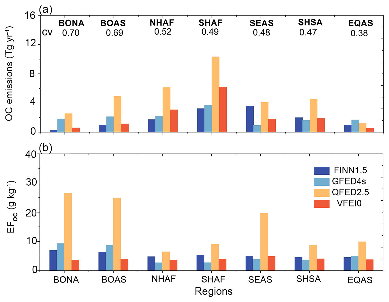
Figure 7(a) Average annual OC emissions of the four biomass burning emissions inventories across seven major BB regions during 2013–2016. The cv, defined as the ratio of the standard deviation to the mean, is the coefficient of variation among the emissions of the four datasets. Panel (b) is the same as (a) but for the emission factor of OC (EFoc).
Unlike the CO EFs, the OC EFs of GFED4s in equatorial regions are largely consistent with the FINN1.5 and VFEI0 emission inventories. Although burning organic-matter-rich soil substrates is generally thought to release large amounts of CO, their ability to release OC is similar to that of vegetation such as shrubs and some forests. Thus, despite CO emissions bias in EQAS being largely affected by peatlands, differences in OC emissions among the four inventories are not significant.
Compared with Pan et al. (2020), it is obvious that the top-down approach will not lead to an increase in emission deviation of the particulate-phase species. The correction of EFs, however, is the root cause of the increased bias in OC emissions. Pan et al. (2020) reported that QFED2.5 and FEER1.0 had the highest global OC emissions, while GFAS1.2 had much lower OC emissions. In this study, the largest OC emission also appears in QFED2.5, but the global total OC emissions of the recently released VFEI0 are relatively low.
4.1 Comparison of simulations with MOPITT CO
One of the main goals of this study is to provide a confidence assessment of the BB emission inventories by comparing model simulations with observations. A comparison between model simulations using different emission inventories and ground-based/satellite-retrieved data for the respective fire seasons (Table 3) of the main BB regions is explored below. In this study, we compared the model results with measurements from two perspectives: the spatial distribution of BB pollutants and the time-varying characteristics of BB pollutants.
Table 3Comparison of CESM-CAM6-simulated CO column averages and satellite-retrieved CO column averages during the fire season. Italics indicate simulated values that are closest to the satellite observations.
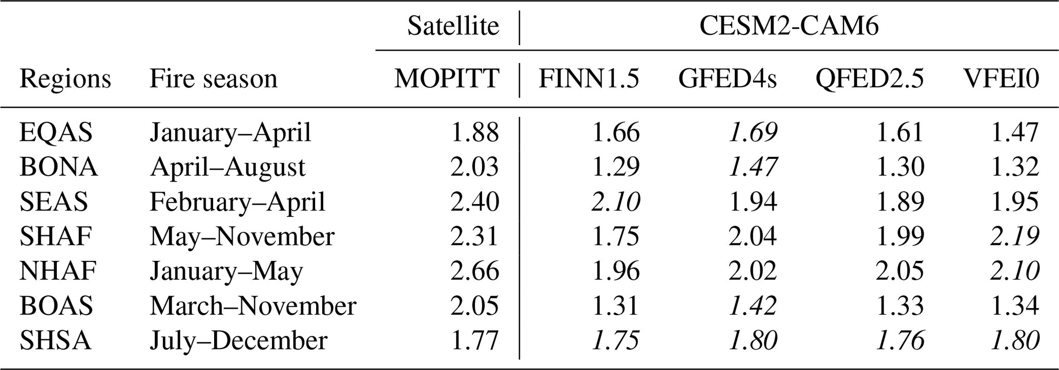
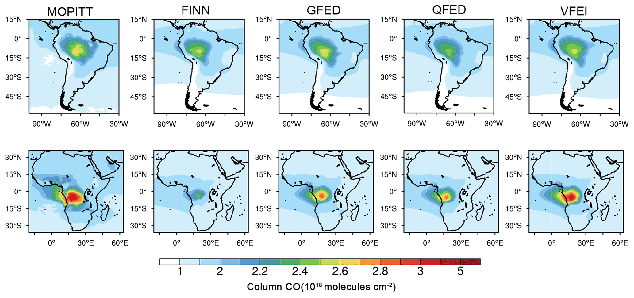
Figure 8Spatial distribution of CO column burdens from MOPITT and CESM2-CAM6 simulations during the fire season (Table 3). The text above each plot identifies the name of the satellite inversion dataset or emission inventory dataset applied by the model, namely FINN1.5, GFED4s, QFED2.5, and VFEI0.
Figure 8 depicts the spatial distribution of CO column burdens in SHSA and SHAF during the fire seasons. In SHSA, the simulated CO column burdens using different emission inventories are all consistent with the spatial distribution pattern of the MOPITT CO column burden, with the peak value located in the Amazon rainforest. However, the central value of the MOPITT CO column burden is as high as 2.8×10¹⁸ , which is slightly higher than the simulated results. Among the four sets of emission inventories, the peak amplitude and spatial distribution of simulated CO column burdens are closest to the satellite-retrieved data after applying GFED4s and VFEI0. In SHAF, however, the model underestimated the peak CO column burden after applying all emission inventories except VFEI0.
In addition to SHSA and SHAF, a comparison of regionally averaged CO column burdens between our simulations and MOPITT CO in major BB regions is also shown in Table 3. In the Northern Hemisphere, our simulations are significantly underestimated compared to MOPITT CO, while those in the Southern Hemisphere are consistent with satellite retrievals. Surprisingly, the simulated spatial distributions and magnitudes of CO in the Southern Hemisphere using the recently released VFEI0 agree very well with observations. In contrast, the underestimation of CO concentrations in the Northern Hemisphere is partly due to uncertainty in anthropogenic emissions, as we assume anthropogenic emissions at 2010 levels, which are lower than those during the 2013–2016 period.
Note that simulated CO concentrations are 30 %–40 % lower than MOPITT CO at high latitudes. Besides the impact of emission inventories, there are also large uncertainties in satellite-retrieved CO concentrations (Lin et al., 2020a; Pan et al., 2020). In addition, OH loss, long-range transport, and photochemical reactions involved in the CESM2-CAM6 model simulations also lead to uncertainties in simulated CO. For example, MOZART-4x contains an additional OH oxidation pathway for CO, which may lead to lower CO concentrations (Lamarque et al., 2012; He and Zhang, 2014; Barré et al., 2015; Brown-Steiner et al., 2018; Emmons et al., 2020). In comparison, the simulated CO using GFED4s is closest to the MOPITT CO value in terms of spatial distribution and peak magnitude at high latitudes in the Northern Hemisphere, which is superior to other emission inventories.
4.2 Comparison of simulations with MODIS AOD
We compared MODIS-derived aerosol optical depth (AOD) data with simulated AOD in major BB areas. Figure 9 shows the spatial distribution of AOD in SHSA and SHAF during their fire seasons. The simulated AOD is significantly higher than the MODIS AOD in SHSA. Note that primary organic aerosols (POAs) associated with BB account for only 15 %–23 % of the total AOD in the Amazon, while secondary organic aerosols (SOAs) account for approximately 50 % of the total AOD. Furthermore, overestimation of simulated AOD occurs throughout the year, not just during the fire season. Considering the high biogenic emissions in this region, the overestimation of AOD could be attributed to the formation of biogenic SOA (He et al., 2015; Tilmes et al., 2019). In SHAF, the spatial distribution and magnitude of simulated AOD using GFED4s and VFEI0 are close to those of the MODIS AOD. In comparison, our results show that AOD is significantly underestimated using FINN1.5 but largely overestimated using QFED2.5.
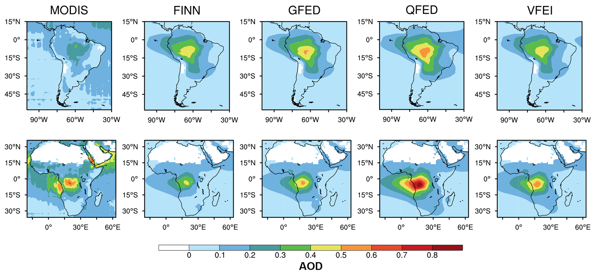
Figure 9The same as Fig. 8 but for AOD.
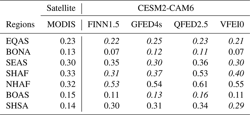
Table 4 shows the mean values of model-simulated AOD and satellite measurements for each region during its fire season. The influence of the BB emission inventory has little effect on the simulated AOD value in the Southern Hemisphere, and the regional average AOD deviation is within 20 %. In contrast, the average deviation of simulated AOD driven by the four BB inventories can be as high as 40 % in the high latitudes of the Northern Hemisphere. Comparatively, GFED4s and QFED2.5 are more suited to high latitudes in the Northern Hemisphere, whereas VFEI0 is the most suitable for the Southern Hemisphere for AOD simulations. In Africa, QFED2.5 is not recommended due to its considerable overestimation.
Table 4The same as Table 3 but for AOD. Italics indicate simulated values that are closest to the satellite observations.
4.3 Comparison of simulations with ground-based measurements
In the above sections, we merely discuss the spatial distribution and the magnitude of pollutants during fire seasons. To further analyze whether each dataset can effectively capture the instantaneous combustion of BB, we compared the value of simulated daily AOD with that of ground-based observations (Fig. 10). To be more representative, we selected stations in each BB region with a large amount of data during the fire seasons, allowing for a comprehensive assessment of the global BB emission inventories. The specific locations of the 12 selected AERONET sites are shown as red triangles in Fig. 1b.
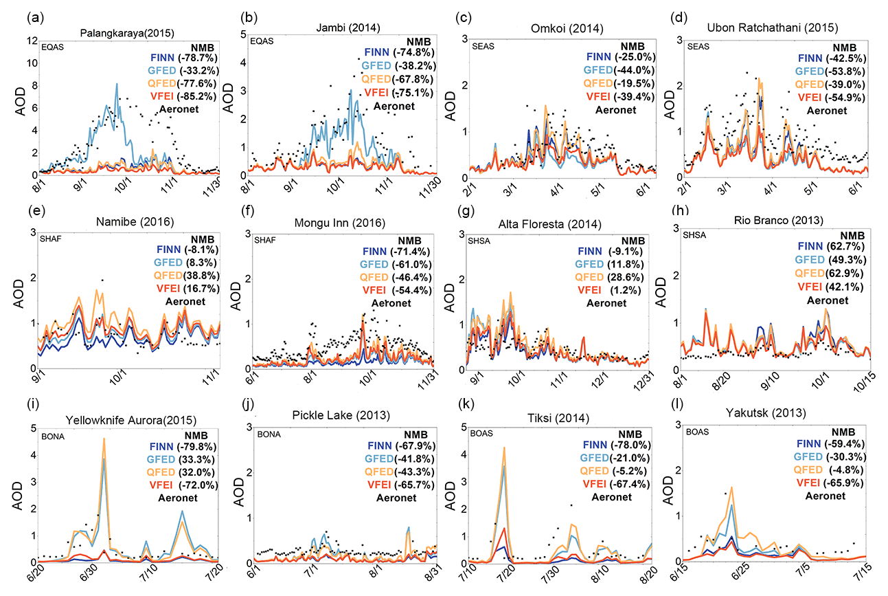
Figure 10Comparison between AOD simulated by CESM2-CAM6 using the four datasets (FINN1.5, GFED4s, QFED2.5, and VFEI0) and AERONET ground-based observations during fire seasons. These AERONET sites are (a) Palangkaraya (2.2° S, 113.9° E), (b) Jambi (1.6° S, 103.6° E), (c) Omkoi (17.8° N, 98.4° E), (d) Ubon Ratchathani (15.2° N, 104.9° E), (e) Namibe (15.2° S, 12.2° E), (f) Mongu Inn (15.3° S, 23.1° E), (g) Alta Floresta (9.9° S, 56.1° W), (h) Rio Branco (9.9° S, 67.9° W), (i) Yellowknife (Aurora) (62.5° N, 114.4° W), (j) Pickle Lake (51.4° N, 90.2° W), (k) Tiksi (71.6° N, 128.9° E), and (l) Yakutsk (61.7° N, 129.4° E).
At EQAS sites such as Palangkaraya and Jambi, the observed AOD from September to November 2014/2015 is generally higher than 1, with peaks exceeding 5, reflecting the intense BB events (Fig. 10a and b). Only simulations using GFED4s were consistent with observed AOD during strong BB events, with a slight underestimation of 33 %–38 %, while none of the other simulations could capture the BB process. Considering the significant contribution of peatlands to BB emissions in EQAS in GFED4s, our results suggest that it is important to include the burning of organic-matter-rich soils in BB emission inventories. At SEAS sites such as Omkoi and Ubon Ratchathani, the peak AOD occurs from February to April at a value of about 2, and all simulations applying the four emission inventories capture the observed changes in AOD (Fig. 10c and d). However, due to the uncertainty in anthropogenic emissions, the simulated AOD is usually smaller than the actual observed value in EQAS. Note that simulations using QFED2.5 are the most consistent with observed AOD during intense biomass burning events.
At the Namibe station of SHAF (Fig. 10e), the simulated AOD agrees best with the measured results after using FINN1.5 and GFED2.5, with normalized mean bias (NMB) values within ± 8 %, indicating these two emission inventories can characterize the day-to-day variability of the intense BB process. However, Namibe is located downwind of the dust source, and dust aerosols contribute more than 50 % to the total AOD in this area. To better evaluate the performance of the four BB emission inventories in SHAF, we chose another site, Mongu Inn, located in the interior of southern hemispheric Africa, where dust and sea salt accounted for 20 %–30 % of the total AOD. At Mongu Inn, all simulations underestimate AOD by 46 %–71 %, and only the QFED2.5 and VFEI0 emission inventories can capture a few peaks during intense biomass burning events (Fig. 10f). In SHSA, while Figs. 9 and 10h show an overall overestimation of simulated AOD compared to MODIS AOD, at the Brazilian Alta Floresta site east of the Amazon, simulated AOD agrees very well with the ground-based observations (Fig. 10g). In general, the simulations using the VFEI0 emission inventory for the Southern Hemisphere are close to the measurements.
At high latitudes, simulations driven by GFED4s and QFED2.5 better capture the observed peak AOD, with regional NMB values of less than 40 % (Fig. 10i–l), suggesting that these two simulations can reproduce the intense BB process. In contrast, FINN1.5 and VFEI0 are obviously not suitable for describing the BB process in these sites, and the simulated AOD is underestimated by 60 %–80 %.
In this study, we examine four commonly used BB emission inventories (two bottom-up inventories (GFED4s and FINN1.5) and two top-down inventories (QFED2.5 and VFEI0)) to better understand the uncertainties associated with BB emissions. We analyze variations in CO and OC emissions across seven major BB regions worldwide from 2013 to 2016. We explore the differences between gaseous and particulate emission inventories, quantifying the impact of vegetation classification, cloud cover, and emission factors on inventory bias. Additionally, we apply these inventories to the global model CESM2-CAM6 to assess the model's performance in simulating pollutants against satellite and ground-based observations.
The total global CO emissions exhibit significant variability among the four inventories, with annual averages ranging from 252 to 336 Tg and a maximum deviation rate exceeding 30 %. In certain regions such as BONA, changes in CO emissions are even larger – GFED4s emits 5.8 times more CO than FINN1.5. DM is identified as the primary contributor to variance among BB emission inventories, accounting for 50 %–80 % of regional bias, while comprehensive EFs contribute the remaining 20 %–50 %. Interestingly, the contributions of DM and comprehensive EFs to emission inventory differences are comparable across equatorial regions and Northern Hemisphere high latitudes.
The uncertainty in DM arises from underlying fuel consumption and burned area, linked to the vegetation classification, fire detection product algorithm, and cloud/smoke masking. Vegetation classification significantly impacts fuel loading and the fraction of biomass burned, with discrepancies contributing to biases in fuel consumption. In regions at both low and high latitudes (except Southeast Asia), FINN1.5 exhibits a fuel consumption term that is less than 50 % of GFED4s, with the vegetation classification methodology contributing primarily to this bias. Different fire detection products introduce bias in estimated burned area, affecting uncertainty in DM. Satellite transit/cloud obscuration influences DM by affecting burned area/fire radiative energy. Cloud cover at high latitudes substantially impacts emission uncertainty, with bias increasing by 20 % in July in BONA with higher cloud fraction.
We extend our analysis to particulate pollutants, using OC emissions as an example. Global average annual OC emissions vary widely among the four inventories, ranging from 14.9 to 42.9 Tg, demonstrating greater variability than gaseous species like CO. BB OC emissions exhibit large variability at high latitudes in the Northern Hemisphere, with QFED2.5 adjusting emission factors based on satellite aerosol optical thickness (AOD) to enhance particulate matter emissions.
Applying four BB emission inventories to CESM2-CAM6, we compare model-simulated CO column concentrations with the MOPITT satellite inversion CO column concentrations. According to our simulations, CO simulated using GFED4s is closest to satellite observations in almost all regions except southern Asia and Africa. We also compared model results with AOD retrieved from MODIS satellites or measured by AERONET. Simulated AOD at high northern latitudes is often underestimated when using current mainstream BB emission inventories. For example, the simulated regional average AOD is 8 %–46 % lower than MODIS in North America. Unlike the high latitudes, the simulated AOD is significantly overestimated at the Equator, and the regional average AOD simulated by the model in northern hemispheric Africa is 66 %–91 % higher than that simulated by MODIS. In addition, comparing model-simulated AOD with AERONET ground-based observations, we find that GFED4s performs best in EQAS for daily variability during intense burning. In SEAS, although FINN1.5 can better represent the magnitude of the overall OC emissions in the BB season, QFED2.5 can capture the day-to-day variation characteristics of intense combustion. In the Southern Hemisphere, the latest VFEI0 emission inventory performs well, and the simulated AOD is able to capture the BB processes.
Our study assesses the global applicability of BB emission inventories and has some implications for future studies. Overall, the GFED4s and QFED2.5 inventories for the northern high latitudes capture the magnitude of and daily variation in OC emitted throughout the BB season. These two emission inventories outperformed the others when applied to studies of interactions between BB aerosol and weather/climate. In the Southern Hemisphere, the spatial distribution and daily variation characteristics of CO and AOD simulated by the model are closest to the observed values when the latest VFEI0 emission inventory is applied. For the Equator, the situation is more complicated, and we recommend combining emission inventories according to the research objectives. For example, GFED4s performs best in day-to-day changes during intense burning in equatorial Asia. In Southeast Asia, combining OC magnitude in FINN1.5 and daily variation in QFED2.5 is the optimal choice.
It is worth noting that emission factors (as listed in Table 2) significantly contribute to the differences in BB emissions. However, actual emission factors vary widely depending on the different states of combustion (Pokhrel et al., 2021). Further study is needed to understand the impact of combustion efficiency on the BB EFs and optimize them.
The GFED4s emission datasets are available from https://doi.org/10.3334/ORNLDAAC/1293 (Randerson et al., 2018). The FINN1.5 emissions can be accessed from NCAR's Atmospheric Chemistry Observations and Modeling repository https://www.acom.ucar.edu/Data/fire/ (last access: 16 August 2023, Wiedinmyer et al., 2011). The QFED2.5 emissions are available from NASA's Center for Climate Simulation public repository at https://portal.nccs.nasa.gov/datashare/iesa/aerosol/emissions/QFED/v2.5r1/ (last access: 16 August 2023, Darmenov et al., 2015). The VFEI0 emissions can be accessed at https://doi.org/10.5281/zenodo.6474058 (last access: 16 August 2023, Ferrada, 2022). MODIS AOD are available from https://doi.org/10.5067/MODIS/MOD08_D3.061 (last access: 16 August 2023, Platnick et al., 2015a), and cloud fraction can be accessed at https://doi.org/10.5067/MODIS/MOD06_L2.061 (last access: 16 August 2023, Platnick et al., 2015b). MODIS Collection 61 NRT Hotspot/Active Fire Detections MCD14DL are available from https://doi.org/10.5067/FIRMS/MODIS/MCD14DL.NRT.0061 (last access: 16 August 2023, Giglio et al., 2018). MOPITT CO can be obtained from https://doi.org/10.5067/TERRA/MOPITT/MOP03JM.009 (last access: 16 August 2023, NASA/LARC/SD/ASDC, 2024). The AERONET data can be accessed at https://aeronet.gsfc.nasa.gov/cgi-bin/webtool_aod_v3 (last access: 10 May 2022, Giles et al., 2019). The Modern-Era Retrospective analysis for Research and Applications, version 2 (MERRA-2) reanalysis datasets used in this study are available from https://doi.org/10.5067/SUOQESM06LPK (last access: 21 May 2020, GMAO, 2015). Additional data and scripts related to the modeling results are available at https://zenodo.org/records/10939422 (last access: 8 April 2024, Hua, 2024).
The supplement related to this article is available online at: https://doi.org/10.5194/acp-24-6787-2024-supplement.
SL and AD designed the research, WH and SL conducted the data analysis and model simulations, and WH and SL took the lead in writing the paper with contributions from all authors.
The contact author has declared that none of the authors has any competing interests.
Publisher's note: Copernicus Publications remains neutral with regard to jurisdictional claims made in the text, published maps, institutional affiliations, or any other geographical representation in this paper. While Copernicus Publications makes every effort to include appropriate place names, the final responsibility lies with the authors.
We appreciate that the 12 sites used in this study are made accessible by the AERONET networks. We sincerely thank the site PIs and data managers of those networks. We acknowledge the use of data and/or imagery from NASA's Fire Information for Resource Management System (FIRMS) (https://earthdata.nasa.gov/firms, last access: 6 May 2022), part of NASA's Earth Observing System Data and Information System (EOSDIS).
This research has been supported by the National Natural Science Foundation of China (grant nos. 42325506, 42075095, 42105095) and the international cooperation project of the Jiangsu Provincial Science and Technology Agency (BZ2017066).
This paper was edited by N'Datchoh Evelyne Touré and reviewed by two anonymous referees.
Adams, C., McLinden, C. A., Shephard, M. W., Dickson, N., Dammers, E., Chen, J., Makar, P., Cady-Pereira, K. E., Tam, N., Kharol, S. K., Lamsal, L. N., and Krotkov, N. A.: Satellite-derived emissions of carbon monoxide, ammonia, and nitrogen dioxide from the 2016 Horse River wildfire in the Fort McMurray area, Atmos. Chem. Phys., 19, 2577–2599, https://doi.org/10.5194/acp-19-2577-2019, 2019.
Akagi, S. K., Yokelson, R. J., Wiedinmyer, C., Alvarado, M. J., Reid, J. S., Karl, T., Crounse, J. D., and Wennberg, P. O.: Emission factors for open and domestic biomass burning for use in atmospheric models, Atmos. Chem. Phys., 11, 4039–4072, https://doi.org/10.5194/acp-11-4039-2011, 2011.
Alencar, A., Nepstad, D., and Moutinho, P.: Carbon emissions associated with forest fires in Brazil, in: Tropical Deforestation and Climate Change, IPAM: Belém, Portugal, p. 23, 2005.
Alvarado, M. J., Logan, J. A., Mao, J., Apel, E., Riemer, D., Blake, D., Cohen, R. C., Min, K.-E., Perring, A. E., Browne, E. C., Wooldridge, P. J., Diskin, G. S., Sachse, G. W., Fuelberg, H., Sessions, W. R., Harrigan, D. L., Huey, G., Liao, J., Case-Hanks, A., Jimenez, J. L., Cubison, M. J., Vay, S. A., Weinheimer, A. J., Knapp, D. J., Montzka, D. D., Flocke, F. M., Pollack, I. B., Wennberg, P. O., Kurten, A., Crounse, J., Clair, J. M. St., Wisthaler, A., Mikoviny, T., Yantosca, R. M., Carouge, C. C., and Le Sager, P.: Nitrogen oxides and PAN in plumes from boreal fires during ARCTAS-B and their impact on ozone: an integrated analysis of aircraft and satellite observations, Atmos. Chem. Phys., 10, 9739–9760, https://doi.org/10.5194/acp-10-9739-2010, 2010.
Andreae, M. and Rosenfeld, D.: Aerosol–cloud–precipitation interactions. Part 1. The nature and sources of cloud-active aerosols, Earth-Sci. Rev., 89, 13–41, 2008.
Andreae, M. O.: Emission of trace gases and aerosols from biomass burning – an updated assessment, Atmos. Chem. Phys., 19, 8523–8546, https://doi.org/10.5194/acp-19-8523-2019, 2019.
Andreae, M. O. and Merlet, P.: Emission of trace gases and aerosols from biomass burning, Global Biogeochem. Cy., 15, 955–966, 2001.
Arellano Jr., A. F. and Hess, P. G.: Sensitivity of top-down estimates of CO sources to GCTM transport, Geophys. Res. Lett., 33, L21807, https://doi.org/10.1029/2006GL027371, 2006.
Arellano Jr., A. F., Kasibhatla, P. S., Giglio, L., van der Werf, G. R., and Randerson, J. T.: Top-down estimates of global CO sources using MOPITT measurements, Geophys. Res. Lett., 31, L01104, https://doi.org/10.1029/2003GL018609, 2004.
Balshi, M. S., McGuire, A. D., Duffy, P., Flannigan, M., Kicklighter, D. W., and Melillo, J.: Vulnerability of carbon storage in North American boreal forests to wildfires during the 21st century, Glob. Change Biol., 15, 1491–1510, 2009.
Barré, J., Gaubert, B., Arellano, A. F., Worden, H. M., Edwards, D. P., Deeter, M. N., Anderson, J. L., Raeder, K., Collins, N., and Tilmes, S.: Assessing the impacts of assimilating IASI and MOPITT CO retrievals using CESM-CAM-chem and DART, J. Geophys. Res.-Atmos., 120, 10501–10529, 2015.
Beck, H. E., Zimmermann, N. E., McVicar, T. R., Vergopolan, N., Berg, A., and Wood, E. F.: Present and future Köppen-Geiger climate classification maps at 1 km resolution, Scientific Data, 5, 1–12, 2018.
Bian, H., Chin, M., Kawa, S., Duncan, B., Arellano, A., and Kasibhatla, P.: Sensitivity of global CO simulations to uncertainties in biomass burning sources, J. Geophys. Res.-Atmos., 112, D23308, https://doi.org/10.1029/2006JD008376, 2007.
Boschetti, L., Roy, D. P., Justice, C. O., and Humber, M. L.: MODIS–Landsat fusion for large area 30 m burned area mapping, Remote Sens. Environ., 161, 27–42, 2015.
Boschetti, L., Roy, D. P., Giglio, L., Huang, H., Zubkova, M., and Humber, M. L.: Global validation of the collection 6 MODIS burned area product, Remote Sens. Environ., 235, 111490, https://doi.org/10.1016/j.rse.2019.111490, 2019.
Boucher, O., Randall, D., Artaxo, P., Bretherton, C., Feingold, G., Forster, P., Kerminen, V.-M., Kondo, Y., Liao, H., Lohmann, U., Rasch, P., Satheesh, S. K., Sherwood, S., Stevens, B., and Zhang, X. Y.: Clouds and aerosols, Climate change 2013: The physical science basis, Contribution of working group I to the fifth assessment report of the intergovernmental panel on climate change, Cambridge University Press, 571–657, https://doi.org/10.1017/CBO9781107415324.016, 2013.
Brando, P. M., Soares-Filho, B., Rodrigues, L., Assunção, A., Morton, D., Tuchschneider, D., Fernandes, E., Macedo, M., Oliveira, U., and Coe, M.: The gathering firestorm in southern Amazonia, Science Advances, 6, eaay1632, https://doi.org/10.1126/sciadv.aay1632, 2020.
Brown-Steiner, B., Selin, N. E., Prinn, R., Tilmes, S., Emmons, L., Lamarque, J.-F., and Cameron-Smith, P.: Evaluating simplified chemical mechanisms within present-day simulations of the Community Earth System Model version 1.2 with CAM4 (CESM1.2 CAM-chem): MOZART-4 vs. Reduced Hydrocarbon vs. Super-Fast chemistry, Geosci. Model Dev., 11, 4155–4174, https://doi.org/10.5194/gmd-11-4155-2018, 2018.
Carter, T. S., Heald, C. L., Jimenez, J. L., Campuzano-Jost, P., Kondo, Y., Moteki, N., Schwarz, J. P., Wiedinmyer, C., Darmenov, A. S., da Silva, A. M., and Kaiser, J. W.: How emissions uncertainty influences the distribution and radiative impacts of smoke from fires in North America, Atmos. Chem. Phys., 20, 2073–2097, https://doi.org/10.5194/acp-20-2073-2020, 2020.
Chen, Y., Li, Q., Randerson, J. T., Lyons, E. A., Kahn, R. A., Nelson, D. L., and Diner, D. J.: The sensitivity of CO and aerosol transport to the temporal and vertical distribution of North American boreal fire emissions, Atmos. Chem. Phys., 9, 6559–6580, https://doi.org/10.5194/acp-9-6559-2009, 2009.
Christian, T. J., Kleiss, B., Yokelson, R. J., Holzinger, R., Crutzen, P. J., Hao, W. M., Saharjo, B. H., and Ward, D. E.: Comprehensive laboratory measurements of biomass - burning emissions: 1. Emissions from Indonesian, African, and other fuels, J. Geophys. Res.-Atmos., 108, 4719, https://doi.org/10.1029/2003JD003704, 2003.
Christian, K., Wang, J., Ge, C., Peterson, D., Hyer, E., Yorks, J., and McGill, M.: Radiative forcing and stratospheric warming of pyrocumulonimbus smoke aerosols: First modeling results with multisensor (EPIC, CALIPSO, and CATS) views from space, Geophys. Res. Lett., 46, 10061–10071, 2019.
Cochrane, M. A.: Fire science for rainforests, Nature, 421, 913–919, 2003.
Cochrane, M. A. and Laurance, W. F.: Fire as a large-scale edge effect in Amazonian forests, J. Trop. Ecol., 18, 311–325, 2002.
Danabasoglu, G., Lamarque, J. F., Bacmeister, J., Bailey, D., DuVivier, A., Edwards, J., Emmons, L., Fasullo, J., Garcia, R., and Gettelman, A.: The community earth system model version 2 (CESM2), J. Adv. Model. Earth Sy., 12, e2019MS001916, https://doi.org/10.1029/2019MS001916, 2020.
Darmenov, A., da Silvia, A., and Koster, R.: The Quick Fire Emissions Dataset (QFED): Documentation of versions 2.1, 2.2 and 2.4, NASA Technical Report Series on Global Modeling and Data Assimilation NASA TM-2015-104606, Volume 38, http://gmao.gsfc.nasa.gov/pubs/docs/Darmenov796.pdf (last access: 8 April 2024), 2015.
Deeter, M., Francis, G., Gille, J., Mao, D., Martínez-Alonso, S., Worden, H., Ziskin, D., Drummond, J., Commane, R., Diskin, G., and McKain, K.: The MOPITT Version 9 CO product: sampling enhancements and validation, Atmos. Meas. Tech., 15, 2325–2344, https://doi.org/10.5194/amt-15-2325-2022, 2022.
Ding, K., Huang, X., Ding, A., Wang, M., Su, H., Kerminen, V.-M., Petäjä, T., Tan, Z., Wang, Z., and Zhou, D.: Aerosol-boundary-layer-monsoon interactions amplify semi-direct effect of biomass smoke on low cloud formation in Southeast Asia, Nat. Commun., 12, 1–9, 2021.
Duncan, B. N., Martin, R. V., Staudt, A. C., Yevich, R., and Logan, J. A.: Interannual and seasonal variability of biomass burning emissions constrained by satellite observations, J. Geophys. Res.-Atmos., 108, ACH 1-1–ACH 1-22, 2003.
Emmons, L. K., Schwantes, R. H., Orlando, J. J., Tyndall, G., Kinnison, D., Lamarque, J.-F., Marsh, D., Mills, M. J., Tilmes, S., Bardeen, C., Buchholz, R. R., Conley, A., Gettelman, A., Garcia, R., Simpson, I., Blake, D. R., Meinardi, S., and Pétron, G.: The Chemistry Mechanism in the Community Earth System Model Version 2 (CESM2), J. Adv. Model. Earth Sy., 12, e2019MS001882, https://doi.org/10.1029/2019MS001882, 2020.
Ferek, R. J., Reid, J. S., Hobbs, P. V., Blake, D. R., and Liousse, C.: Emission factors of hydrocarbons, halocarbons, trace gases and particles from biomass burning in Brazil, J. Geophys. Res.-Atmos., 103, 32107–32118, 1998.
Ferrada, G. A., Zhou, M., Wang, J., Lyapustin, A., Wang, Y., Freitas, S. R., and Carmichael, G. R.: Introducing the VIIRS-based Fire Emission Inventory version 0 (VFEIv0), Geosci. Model Dev., 15, 8085–8109, https://doi.org/10.5194/gmd-15-8085-2022, 2022.
Firms, L.: Collection 6 NRT hotspot/active fire detections MCD14DL, https://earthdata.nasa.gov/firms, last access: 21 June 2017.
Freitas, S., Longo, K., and Andreae, M.: Impact of including the plume rise of vegetation fires in numerical simulations of associated atmospheric pollutants, Geophys. Res. Lett., 33, L17808, https://doi.org/10.1029/2006GL026608, 2006.
Freitas, S. R., Longo, K. M., Trentmann, J., and Latham, D.: Technical Note: Sensitivity of 1-D smoke plume rise models to the inclusion of environmental wind drag, Atmos. Chem. Phys., 10, 585–594, https://doi.org/10.5194/acp-10-585-2010, 2010.
GMAO: Global Modeling and Assimilation Office (GMAO), MERRA-2 tavg3_3d_mst_Ne: 3d,3-Hourly,Time-Averaged,Model-Level Edge,Assimilation,Moist Processes Diagnostics V5.12.4, Greenbelt, MD, USA, Goddard Earth Sciences Data and Information Services Center (GES DISC), https://doi.org/10.5067/JRUZ3SJ3ZJ72, 2015.
Gibson, C. M., Chasmer, L. E., Thompson, D. K., Quinton, W. L., Flannigan, M. D., and Olefeldt, D.: Wildfire as a major driver of recent permafrost thaw in boreal peatlands, Nat. Commun., 9, 3041, https://doi.org/10.1038/s41467-018-05457-1, 2018.
Giglio, L., Randerson, J. T., and van der Werf, G. R.: Analysis of daily, monthly, and annual burned area using the fourth-generation global fire emissions database (GFED4), J. Geophys. Res.-Biogeo., 118, 317–328, 2013.
Giles, D. M., Sinyuk, A., Sorokin, M. G., Schafer, J. S., Smirnov, A., Slutsker, I., Eck, T. F., Holben, B. N., Lewis, J. R., Campbell, J. R., Welton, E. J., Korkin, S. V., and Lyapustin, A. I.: Advancements in the Aerosol Robotic Network (AERONET) Version 3 database – automated near-real-time quality control algorithm with improved cloud screening for Sun photometer aerosol optical depth (AOD) measurements, Atmos. Meas. Tech., 12, 169–209, https://doi.org/10.5194/amt-12-169-2019, 2019.
Guenther, A. B., Jiang, X., Heald, C. L., Sakulyanontvittaya, T., Duhl, T., Emmons, L. K., and Wang, X.: The Model of Emissions of Gases and Aerosols from Nature version 2.1 (MEGAN2.1): an extended and updated framework for modeling biogenic emissions, Geosci. Model Dev., 5, 1471–1492, https://doi.org/10.5194/gmd-5-1471-2012, 2012.
He, J. and Zhang, Y.: Improvement and further development in CESM/CAM5: gas-phase chemistry and inorganic aerosol treatments, Atmos. Chem. Phys., 14, 9171–9200, https://doi.org/10.5194/acp-14-9171-2014, 2014.
He, J., Zhang, Y., Tilmes, S., Emmons, L., Lamarque, J.-F., Glotfelty, T., Hodzic, A., and Vitt, F.: CESM/CAM5 improvement and application: comparison and evaluation of updated CB05_GE and MOZART-4 gas-phase mechanisms and associated impacts on global air quality and climate, Geosci. Model Dev., 8, 3999–4025, https://doi.org/10.5194/gmd-8-3999-2015, 2015.
Hoelzemann, J. J., Schultz, M. G., Brasseur, G. P., Granier, C., and Simon, M.: Global Wildland Fire Emission Model (GWEM): Evaluating the use of global area burnt satellite data, J. Geophys. Res.-Atmos., 109, D14S04, https://doi.org/10.1029/2003JD003666, 2004.
Hoesly, R. M., Smith, S. J., Feng, L., Klimont, Z., Janssens-Maenhout, G., Pitkanen, T., Seibert, J. J., Vu, L., Andres, R. J., Bolt, R. M., Bond, T. C., Dawidowski, L., Kholod, N., Kurokawa, J.-I., Li, M., Liu, L., Lu, Z., Moura, M. C. P., O'Rourke, P. R., and Zhang, Q.: Historical (1750–2014) anthropogenic emissions of reactive gases and aerosols from the Community Emissions Data System (CEDS), Geosci. Model Dev., 11, 369–408, https://doi.org/10.5194/gmd-11-369-2018, 2018.
Holben, B. N., Eck, T. F., Slutsker, I. A., Tanre, D., Buis, J., Setzer, A., Vermote, E., Reagan, J. A., Kaufman, Y., and Nakajima, T.: AERONET – A federated instrument network and data archive for aerosol characterization, Remote Sens. Environ., 66, 1–16, 1998.
Hua, W.: Diagnosing uncertainties in global biomass burning emission inventories and their impact on modeled air pollutants, Zenodo [data set], https://zenodo.org/records/10939422 (last access: 8 April 2024), 2024.
Huang, X., Ding, K., Liu, J., Wang, Z., Tang, R., Xue, L., Wang, H., Zhang, Q., Tan, Z.-M., Fu, C., Davis, S. J., Andreae, M. O., and Ding, A.: Smoke-weather interaction affects extreme wildfires in diverse coastal regions, Science, 379, 457–461, https://doi.org/10.1126/science.add9843, 2023.
Ichoku, C. and Ellison, L.: Global top-down smoke-aerosol emissions estimation using satellite fire radiative power measurements, Atmos. Chem. Phys., 14, 6643–6667, https://doi.org/10.5194/acp-14-6643-2014, 2014.
Jiang, Y., Yang, X.-Q., Liu, X., Qian, Y., Zhang, K., Wang, M., Li, F., Wang, Y., and Lu, Z.: Impacts of wildfire aerosols on global energy budget and climate: The role of climate feedbacks, J. Climate, 33, 3351–3366, 2020.
Junghenn Noyes, K. T., Kahn, R. A., Limbacher, J. A., and Li, Z.: Canadian and Alaskan wildfire smoke particle properties, their evolution, and controlling factors, from satellite observations, Atmos. Chem. Phys., 22, 10267–10290, https://doi.org/10.5194/acp-22-10267-2022, 2022.
Kaiser, J., Flemming, J., Schultz, M., Suttie, M., and Wooster, M.: The MACC global fire assimilation system: First emission products (GFASv0), Tech. Memo. 596, ECMWF, Reading, UK, https://doi.org/10.21957/61tm14m3j, 2009.
Kaiser, J. W., Heil, A., Andreae, M. O., Benedetti, A., Chubarova, N., Jones, L., Morcrette, J.-J., Razinger, M., Schultz, M. G., Suttie, M., and van der Werf, G. R.: Biomass burning emissions estimated with a global fire assimilation system based on observed fire radiative power, Biogeosciences, 9, 527–554, https://doi.org/10.5194/bg-9-527-2012, 2012.
Kasischke, E. S. and Bruhwiler, L. P.: Emissions of carbon dioxide, carbon monoxide, and methane from boreal forest fires in 1998, J. Geophys. Res.-Atmos., 107, FFR 2-1–FFR 2-14, 2002.
Kiely, L., Spracklen, D., Arnold, S., Papargyropoulou, E., Conibear, L., Wiedinmyer, C., Knote, C., and Adrianto, H.: Assessing costs of Indonesian fires and the benefits of restoring peatland, Nat. Commun., 12, 7044, https://doi.org/10.1038/s41467-021-27353-x, 2021.
Knorr, W., Dentener, F., Hantson, S., Jiang, L., Klimont, Z., and Arneth, A.: Air quality impacts of European wildfire emissions in a changing climate, Atmos. Chem. Phys., 16, 5685–5703, https://doi.org/10.5194/acp-16-5685-2016, 2016.
Lamarque, J.-F., Emmons, L. K., Hess, P. G., Kinnison, D. E., Tilmes, S., Vitt, F., Heald, C. L., Holland, E. A., Lauritzen, P. H., Neu, J., Orlando, J. J., Rasch, P. J., and Tyndall, G. K.: CAM-chem: description and evaluation of interactive atmospheric chemistry in the Community Earth System Model, Geosci. Model Dev., 5, 369–411, https://doi.org/10.5194/gmd-5-369-2012, 2012.
Lin, C., Cohen, J. B., Wang, S., and Lan, R.: Application of a combined standard deviation and mean based approach to MOPITT CO column data, and resulting improved representation of biomass burning and urban air pollution sources, Remote Sens. Environ., 241, 111720, https://doi.org/10.1016/j.rse.2020.111720, 2020a.
Lin, C., Cohen, J. B., Wang, S., Lan, R., and Deng, W.: A new perspective on the spatial, temporal, and vertical distribution of biomass burning: quantifying a significant increase in CO emissions, Environ. Res. Lett., 15, 104091, https://doi.org/10.1088/1748-9326/abaa7a, 2020b.
Liousse, C., Guillaume, B., Grégoire, J. M., Mallet, M., Galy, C., Pont, V., Akpo, A., Bedou, M., Castéra, P., Dungall, L., Gardrat, E., Granier, C., Konaré, A., Malavelle, F., Mariscal, A., Mieville, A., Rosset, R., Serça, D., Solmon, F., Tummon, F., Assamoi, E., Yoboué, V., and Van Velthoven, P.: Updated African biomass burning emission inventories in the framework of the AMMA-IDAF program, with an evaluation of combustion aerosols, Atmos. Chem. Phys., 10, 9631–9646, https://doi.org/10.5194/acp-10-9631-2010, 2010.
Liu, L., Cheng, Y., Wang, S., Wei, C., Pöhlker, M. L., Pöhlker, C., Artaxo, P., Shrivastava, M., Andreae, M. O., Pöschl, U., and Su, H.: Impact of biomass burning aerosols on radiation, clouds, and precipitation over the Amazon: relative importance of aerosol–cloud and aerosol–radiation interactions, Atmos. Chem. Phys., 20, 13283–13301, https://doi.org/10.5194/acp-20-13283-2020, 2020.
Liu, T., Mickley, L. J., Marlier, M. E., DeFries, R. S., Khan, M. F., Latif, M. T., and Karambelas, A.: Diagnosing spatial biases and uncertainties in global fire emissions inventories: Indonesia as regional case study, Remote Sens. Environ., 237, 111557, https://doi.org/10.1016/j.rse.2019.111557, 2020.
Liu, X., Ma, P.-L., Wang, H., Tilmes, S., Singh, B., Easter, R. C., Ghan, S. J., and Rasch, P. J.: Description and evaluation of a new four-mode version of the Modal Aerosol Module (MAM4) within version 5.3 of the Community Atmosphere Model, Geosci. Model Dev., 9, 505–522, https://doi.org/10.5194/gmd-9-505-2016, 2016.
Liu, Y., Zhang, K., Qian, Y., Wang, Y., Zou, Y., Song, Y., Wan, H., Liu, X., and Yang, X.-Q.: Investigation of short-term effective radiative forcing of fire aerosols over North America using nudged hindcast ensembles, Atmos. Chem. Phys., 18, 31–47, https://doi.org/10.5194/acp-18-31-2018, 2018.
McMeeking, G. R., Kreidenweis, S. M., Baker, S., Carrico, C. M., Chow, J. C., Collett Jr., J. L., Hao, W. M., Holden, A. S., Kirchstetter, T. W., and Malm, W. C.: Emissions of trace gases and aerosols during the open combustion of biomass in the laboratory, J. Geophys. Res.-Atmos., 114, D19210, https://doi.org/10.1029/2009JD011836, 2009.
Mieville, A., Granier, C., Liousse, C., Guillaume, B., Mouillot, F., Lamarque, J.-F., Grégoire, J.-M., and Pétron, G.: Emissions of gases and particles from biomass burning during the 20th century using satellite data and an historical reconstruction, Atmos. Environ., 44, 1469–1477, 2010.
NASA/LARC/SD/ASDC: MOPITT CO gridded monthly means (Near and Thermal Infrared Radiances) V009, NASA Langley Atmospheric Science Data Center DAAC [data set], https://doi.org/10.5067/TERRA/MOPITT/MOP03JM.009, 2024.
Neu, J. L. and Prather, M. J.: Toward a more physical representation of precipitation scavenging in global chemistry models: cloud overlap and ice physics and their impact on tropospheric ozone, Atmos. Chem. Phys., 12, 3289–3310, https://doi.org/10.5194/acp-12-3289-2012, 2012.
Olson, D. M., Dinerstein, E., Wikramanayake, E. D., Burgess, N. D., Powell, G. V., Underwood, E. C., D'Amico, J. A., Itoua, I., Strand, H. E., and Morrison, J. C.: Terrestrial Ecoregions of the World: A New Map of Life on EarthA new global map of terrestrial ecoregions provides an innovative tool for conserving biodiversity, BioScience, 51, 933–938, 2001.
Page, S. E., Siegert, F., Rieley, J. O., Boehm, H.-D. V., Jaya, A., and Limin, S.: The amount of carbon released from peat and forest fires in Indonesia during 1997, Nature, 420, 61–65, 2002.
Pan, X., Ichoku, C., Chin, M., Bian, H., Darmenov, A., Colarco, P., Ellison, L., Kucsera, T., da Silva, A., Wang, J., Oda, T., and Cui, G.: Six global biomass burning emission datasets: intercomparison and application in one global aerosol model, Atmos. Chem. Phys., 20, 969–994, https://doi.org/10.5194/acp-20-969-2020, 2020.
Paton-Walsh, C., Deutscher, N. M., Griffith, D., Forgan, B., Wilson, S., Jones, N., and Edwards, D.: Trace gas emissions from savanna fires in northern Australia, J. Geophys. Res.-Atmos., 115, D16314, https://doi.org/10.1029/2009JD013309, 2010.
Paton-Walsh, C., Emmons, L. K., and Wiedinmyer, C.: Australia's Black Saturday fires–Comparison of techniques for estimating emissions from vegetation fires, Atmos. Environ., 60, 262–270, 2012.
Platnick, S., Meyer, K. G., King, M. D., Wind, G., Amarasinghe, N., Marchant, B., Thomas Arnold, G., Zhang, Z., Hubanks, P. A., Holz, R. E., Yang, P., Ridgway, W. L., and Riedi, J: MODIS Atmosphere L3 Daily Product, NASA MODIS Adaptive Processing System, Goddard Space Flight Center [data set], USA, https://doi.org/10.5067/MODIS/MOD08_D3.061, 2015a.
Platnick, S., Ackerman, S., King, M., Meyer, K., Menzel, W. P., Holz, R. E., Baum, B. A., and Yang, P.: MODIS Atmosphere L2 Cloud Product (06_L2), NASA MODIS Adaptive Processing System, Goddard Space Flight Center [data set], USA, https://doi.org/10.5067/MODIS/MOD06_L2.061, 2015b.
Pokhrel, R. P., Gordon, J., Fiddler, M. N., and Bililign, S.: Impact of combustion conditions on physical and morphological properties of biomass burning aerosol, Aerosol Sci. Tech., 55, 80–91, 2021.
Ramnarine, E., Kodros, J. K., Hodshire, A. L., Lonsdale, C. R., Alvarado, M. J., and Pierce, J. R.: Effects of near-source coagulation of biomass burning aerosols on global predictions of aerosol size distributions and implications for aerosol radiative effects, Atmos. Chem. Phys., 19, 6561–6577, https://doi.org/10.5194/acp-19-6561-2019, 2019.
Randerson, J. T., van der Werf, G. R., Giglio, L., Collztz, G. J., and Kasibhatla, P. S.: Global Fire Emission Database, Version 4.1 (GFEDv4). ORNLDAAC, Oak Ridge, Tennessee, USA, https://doi.org/10.3334/ORNLDAAC/1293, 2018.
Reid, W. V. and Mooney, H. A.: The Millennium Ecosystem Assessment: testing the limits of interdisciplinary and multi-scale science, Curr. Opin. Env. Sust., 19, 40–46, 2016.
Reid, W. V., Mooney, H. A., Cropper, A., Capistrano, D., Carpenter, S. R., Chopra, K., Dasgupta, P., Dietz, T., Duraiappah, A. K., and Hassan, R.: Ecosystems and human well-being-Synthesis: A report of the Millennium Ecosystem Assessment, Island Press, ISBN 1569735972, 2005.
Roy, D. P., Boschetti, L., Justice, C., and Ju, J.: The collection 5 MODIS burned area product – Global evaluation by comparison with the MODIS active fire product, Remote Sens. Environ., 112, 3690–3707, 2008.
Spracklen, D. V., Jimenez, J. L., Carslaw, K. S., Worsnop, D. R., Evans, M. J., Mann, G. W., Zhang, Q., Canagaratna, M. R., Allan, J., Coe, H., McFiggans, G., Rap, A., and Forster, P.: Aerosol mass spectrometer constraint on the global secondary organic aerosol budget, Atmos. Chem. Phys., 11, 12109–12136, https://doi.org/10.5194/acp-11-12109-2011, 2011.
Stockwell, T., Zhao, J., Greenfield, T., Li, J., Livingston, M., and Meng, Y.: Estimating under- and over-reporting of drinking in national surveys of alcohol consumption: identification of consistent biases across four English-speaking countries, Addiction, 111, 1203–1213, 2016.
Tilmes, S., Hodzic, A., Emmons, L., Mills, M., Gettelman, A., Kinnison, D. E., Park, M., Lamarque, J. F., Vitt, F., and Shrivastava, M.: Climate forcing and trends of organic aerosols in the Community Earth System Model (CESM2), J. Adv. Model. Earth Sy., 11, 4323–4351, 2019.
Urbanski, S. P., Hao, W. M., and Nordgren, B.: The wildland fire emission inventory: western United States emission estimates and an evaluation of uncertainty, Atmos. Chem. Phys., 11, 12973–13000, https://doi.org/10.5194/acp-11-12973-2011, 2011.
van der Werf, G. R., Randerson, J. T., Giglio, L., Collatz, G. J., Kasibhatla, P. S., and Arellano Jr., A. F.: Interannual variability in global biomass burning emissions from 1997 to 2004, Atmos. Chem. Phys., 6, 3423–3441, https://doi.org/10.5194/acp-6-3423-2006, 2006.
van der Werf, G. R., Randerson, J. T., Giglio, L., Collatz, G. J., Mu, M., Kasibhatla, P. S., Morton, D. C., DeFries, R. S., Jin, Y., and van Leeuwen, T. T.: Global fire emissions and the contribution of deforestation, savanna, forest, agricultural, and peat fires (1997–2009), Atmos. Chem. Phys., 10, 11707–11735, https://doi.org/10.5194/acp-10-11707-2010, 2010.
van der Werf, G. R., Randerson, J. T., Giglio, L., van Leeuwen, T. T., Chen, Y., Rogers, B. M., Mu, M., van Marle, M. J. E., Morton, D. C., Collatz, G. J., Yokelson, R. J., and Kasibhatla, P. S.: Global fire emissions estimates during 1997–2016, Earth Syst. Sci. Data, 9, 697–720, https://doi.org/10.5194/essd-9-697-2017, 2017.
Vetrita, Y., Cochrane, M. A., Priyatna, M., Sukowati, K. A., and Khomarudin, M. R.: Evaluating accuracy of four MODIS-derived burned area products for tropical peatland and non-peatland fires, Environ. Res. Lett., 16, 035015, https://doi.org/10.1088/1748-9326/abd3d1, 2021.
Warner, J. X., Gille, J. C., Edwards, D. P., Ziskin, D. C., Smith, M. W., Bailey, P. L., and Rokke, L.: Cloud detection and clearing for the Earth Observing System Terra satellite Measurements of Pollution in the Troposphere (MOPITT) experiment, Appl. Optics, 40, 1269–1284, 2001.
Webb, M. J., Andrews, T., Bodas-Salcedo, A., Bony, S., Bretherton, C. S., Chadwick, R., Chepfer, H., Douville, H., Good, P., Kay, J. E., Klein, S. A., Marchand, R., Medeiros, B., Siebesma, A. P., Skinner, C. B., Stevens, B., Tselioudis, G., Tsushima, Y., and Watanabe, M.: The Cloud Feedback Model Intercomparison Project (CFMIP) contribution to CMIP6, Geosci. Model Dev., 10, 359–384, https://doi.org/10.5194/gmd-10-359-2017, 2017.
Westerling, A. L. and Bryant, B.: Climate change and wildfire in California, Climatic Change, 87, 231–249, 2008.
Westerling, A. L., Hidalgo, H. G., Cayan, D. R., and Swetnam, T. W.: Warming and earlier spring increase western US forest wildfire activity, Science, 313, 940–943, 2006.
Wiedinmyer, C., Quayle, B., Geron, C., Belote, A., McKenzie, D., Zhang, X., O'Neill, S., and Wynne, K. K.: Estimating emissions from fires in North America for air quality modeling, Atmos. Environ., 40, 3419–3432, 2006.
Wiedinmyer, C., Akagi, S. K., Yokelson, R. J., Emmons, L. K., Al-Saadi, J. A., Orlando, J. J., and Soja, A. J.: The Fire INventory from NCAR (FINN): a high resolution global model to estimate the emissions from open burning, Geosci. Model Dev., 4, 625–641, https://doi.org/10.5194/gmd-4-625-2011, 2011.
Williams, J. E., van Weele, M., van Velthoven, P. F., Scheele, M. P., Liousse, C., and van Der Werf, G. R.: The impact of uncertainties in African biomass burning emission estimates on modeling global air quality, long range transport and tropospheric chemical lifetimes, Atmosphere, 3, 132–163, 2012.
Yang, Y., Smith, S. J., Wang, H., Mills, C. M., and Rasch, P. J.: Variability, timescales, and nonlinearity in climate responses to black carbon emissions, Atmos. Chem. Phys., 19, 2405–2420, https://doi.org/10.5194/acp-19-2405-2019, 2019.
Yokelson, R. J., Susott, R., Ward, D. E., Reardon, J., and Griffith, D. W. T.: Emissions from smoldering combustion of biomass measured by open-path Fourier transform infrared spectroscopy, J. Geophys. Res.-Atmos., 102, 18865–18877, 1997.
Yu, P., Toon, O. B., Bardeen, C. G., Zhu, Y., Rosenlof, K. H., Portmann, R. W., Thornberry, T. D., Gao, R.-S., Davis, S. M., and Wolf, E. T.: Black carbon lofts wildfire smoke high into the stratosphere to form a persistent plume, Science, 365, 587–590, 2019.
Zhang, Y., Li, Z., Chen, Y., de Leeuw, G., Zhang, C., Xie, Y., and Li, K.: Improved inversion of aerosol components in the atmospheric column from remote sensing data, Atmos. Chem. Phys., 20, 12795–12811, https://doi.org/10.5194/acp-20-12795-2020, 2020.
- Abstract
- Introduction
- Data and methodology
- Comparative analysis of emission inventories
- Model evaluation based on emission inventory application
- Conclusion and discussion
- Data availability
- Author contributions
- Competing interests
- Disclaimer
- Acknowledgements
- Financial support
- Review statement
- References
- Supplement