the Creative Commons Attribution 4.0 License.
the Creative Commons Attribution 4.0 License.
 | 06 Jun 2024
Role of atmospheric aerosols in severe winter fog over the Indo-Gangetic Plain of India: a case study
Chandrakala Bharali
Mary Barth
Rajesh Kumar
Sachin D. Ghude
Vinayak Sinha
Baerbel Sinha
Winter fog and severe aerosol loading in the boundary layer over northern India, particularly in the Indo-Gangetic Plain (IGP), disrupt the daily lives of millions of people in the region. To better understand the role of aerosol–radiation (AR) feedback on the occurrence, spatial extent, and persistence of winter fog, as well as the associated aqueous chemistry in fog in the IGP, several model simulations have been performed using the Weather Research and Forecasting model coupled with Chemistry (WRF-Chem). While WRF-Chem was able to represent the fog formation for the 23–24 December 2017 fog event over the central IGP in comparison to station and satellite observations, the model underestimated PM2.5 concentrations compared to the Central Pollution Control Board (CPCB) of India monitoring network. While evaluating aerosol composition for fog events in the IGP, we found that the WRF-Chem aerosol composition was quite different from measurements obtained during the Winter Fog Experiment (WiFEX) in Delhi, with secondary aerosols, particularly the chloride aerosol fraction, being strongly underpredicted (∼ 66.6 %). Missing emission sources (e.g., industry and residential burning of cow dung and trash) and aerosol and chemistry processes need to be investigated to improve model–observation agreement. By investigating a fog event on 23–24 December 2017 over the central IGP, we found that the aerosol–radiation feedback weakens turbulence, lowers the boundary layer height, and increases PM2.5 concentrations and relative humidity (RH) within the boundary layer. Factors affecting the feedback include loss of aerosols through deposition of cloud droplets and internal mixing of absorbing and scattering aerosols. Aqueous-phase chemistry increases the PM2.5 concentrations, which subsequently affect the aerosol–radiation feedback by both increased mass concentrations and aerosol sizes. With aerosol–radiation interaction and aqueous-phase chemistry, fog formation began 1–2 h earlier and caused a longer fog duration than when these processes were not included in the WRF-Chem simulation. The increase in RH in both experiments was found to be important for fog formation as it promoted the growth of aerosol size through water uptake, increasing the fog water content over the IGP. The results from this study suggest that the aerosol–radiation feedback and secondary aerosol formation play an important role in the air quality and the intensity and lifetime of fog over the IGP, yet other feedbacks, such as aerosol–cloud interactions, need to be quantified.
- Article
(10036 KB) - Full-text XML
-
Supplement
(1835 KB) - BibTeX
- EndNote


The Indo-Gangetic Plain (IGP; 21°35′–32°28′ N latitude and 73°50′–89°49′ E longitude) in the northern part of the Indian subcontinent is one of the most densely populated and heavily polluted regions in southern Asia. The rapid population and economic growth in the IGP region over the last decade have increased air pollution over this region. This is evident from the increasing trend in aerosol optical depth (AOD) and NO2 column concentration over India reported in recent studies (Dey and Di Girolamo, 2011; Ghude et al., 2013; Krishna Moorthy et al., 2013), which has slowed and reversed only recently (Sarkar et al., 2019). The high concentration of aerosols along the IGP and their adverse effects on human health and the environment are increasing (Ghude et al., 2016). Consequently, more than 500 million people living in the IGP breathe air that exceeds the National Ambient Air Quality Standards (NAAQS), which has reduced the life expectancy of these people (Debnath et al., 2022; Lelieveld et al., 2015). Lelieveld et al. (2015) estimated a very high number of premature deaths (0.716 million yr−1) linked to aerosols (PM2.5), thus making southeastern Asia one of the largest regions affected by premature mortality globally.
One of the major environmental concerns in the IGP is the urban air quality during winter, especially over the megacities, e.g., Delhi, located in the northwestern part of the IGP (Ghude et al., 2020; Jena et al., 2021; Sengupta et al., 2022). Several urban air pollution hotspots along the IGP extend from northwest to east with monthly average PM2.5 greater than 200 µg m−3 (NAAQS = 60 µg m−3, 24 h average) in the winter season (Bharali et al., 2019; Krishna et al., 2019). The IGP is dominated mainly by fine-mode particulates, especially over the central to eastern IGP, during the post-monsoon season and winter (Kumar et al., 2018). Biomass burning (agricultural waste burning, domestic heating, etc.) is an important contributor to the observed high PM2.5 loading over the IGP during these seasons (Kulkarni et al., 2020; Pant et al., 2015; Pawar and Sinha, 2022; Anu Rani Sharma et al., 2010; Yadav et al., 2020). Delhi is affected substantially by the emissions from agricultural waste burning in the northwestern states of Punjab and Haryana during the post-monsoon (October–November) season (Badarinath et al., 2009; Jethva et al., 2018; Kumar et al., 2021). Studies showed that PM2.5 increased from ∼ 50 µg m−3 to as high as 300 µg m−3 (Ojha et al., 2020) and that AOD reached 0.98 with the presence of absorbing aerosols (Singh et al., 2018) during the peak biomass burning in the post-monsoon season.
The IGP experiences fog (both radiation and advection fog) every winter after the passage of the synoptic wind system called the “western disturbances”. The majority of fog events in the IGP during December–January are radiation fog (Deshpande et al., 2023; Ghude et al., 2023), formed due to radiative cooling of the surface. The number of low-visibility days due to haze and/or fog formation has been increasing significantly (Ghude et al., 2017; Jenamani, 2007; Singh and Dey, 2012), impacting socioeconomic activities, e.g., aviation (Kulkarni et al., 2019). The increase in the intensity and regional extent of fog over the IGP is consistent with the increasing trend in aerosol concentration due to increasing anthropogenic emissions (Sarkar et al., 2006; Syed et al., 2012).
Several factors control the formation and persistence of fog in the IGP, e.g., stable boundary layer, low temperature, availability of moisture (supplied by the western disturbances and irrigation activities), and the aerosol number and composition (Acharja et al., 2022; Dhangar et al., 2021). It has also been suggested that the atmospheric rivers (moisture incursion from the Arabian Sea) act as a source of water vapor over the IGP, which fuels the intensification of fog and haze (Verma et al., 2022) during winter. The high aerosol concentration in the boundary layer influences fog formation (Gautam et al., 2007; Safai et al., 2019) over the IGP by providing the needed cloud condensation nuclei (CCN) for activation into fog droplets. In addition, aerosols induce surface cooling by reducing solar radiation at the surface while warming the lower troposphere by absorption (Ding et al., 2016; Yu et al., 2002). A reduction in surface-reaching solar radiation by ∼ 19 % has been reported during winter over Kanpur in the IGP (Dey and Tripathi, 2007). The reduced solar flux affects the boundary layer stability and depth by suppressing the thermals and thus further increasing the surface aerosol concentration via aerosol–radiation (AR) feedback, which is very strong over the IGP (Bharali et al., 2019). Kumar et al. (2020) showed that aerosol–radiation feedback significantly improves the accuracy of PM2.5 and temperature forecasts in Delhi. Srivastava et al. (2018) reported that the direct aerosol forcing over polluted regions is very large with values up to −80.0 ± 7.2 W m−2 over the IGP in winter.
Aerosol–radiation interaction determines that the aerosol distribution is critical for the evolution of fog (Bodaballa et al., 2022; Steeneveld et al., 2015), while microphysics is important for fog formation and dispersal (Boutle et al., 2018; Maalick et al., 2016). Although the relationship between the aerosol chemical composition and aerosol activation to CCN has not been fully understood yet, studies have found that the chemical composition and mixing state of aerosols affect the hygroscopicity (κ) of aerosols (Bodaballa et al., 2022; Ma et al., 2013; Moore et al., 2012; F. Zhang et al., 2014). Fog processes involve a complex interplay between local meteorology, radiation, microphysics, and aerosol chemistry, making it difficult to understand the fog lifecycle (Acharja et al., 2022; Maalick et al., 2016; X. Zhang et al., 2014). There is considerable heterogeneity in the spatial and temporal aerosol properties over the IGP and the poor estimates of their mixing state. Therefore, prediction of fog by weather models is still challenging with biases in the onset of fog and its dispersal timings.
Previous studies have focused on the impacts of meteorological conditions, topography, or anthropogenic emissions on the poor air quality and intensification of fog during winter over the IGP (e.g., Hakkim et al., 2019). However, studies on the effect of feedback induced by the aerosols on the meteorological conditions and thus on aerosol concentration are very limited over this region, except for a few abovementioned studies which discuss how the aerosol–radiation feedback favors haze and fog during winter. Moreover, fog can provide a medium for aqueous-phase reactions. While several earlier studies have reported an increase in secondary aerosols during fog over the IGP, a sensitivity study examining the impact of fog on aqueous-phase chemistry has not yet been done over the IGP.
In the present work, we aim to find the suitable chemistry/physics and the meteorology initial/boundary conditions that lead to improved simulations of fog events in the Weather Research and Forecasting model coupled with Chemistry (WRF-Chem; Fast et al., 2006; Grell et al., 2005; Powers et al., 2017). We also explore the role of aerosol–radiation feedback on fog properties as the high aerosol loadings in northern India can impact the heating rates, temperature inversions, and boundary layer height. The role of aqueous chemistry in fog properties and vice versa is also investigated.
Fog formed due to radiative cooling, based on the onset time of fog and low wind speeds (WSs; Deshpande et al., 2023, and references therein), at the surface on both 23 and 24 December 2017 over a widespread region of the IGP (Fig. 1a, b). The fog region is located over an area with high PM2.5 anthropogenic emissions (Fig. 1c). The IGP is a large region with varying meteorology and aerosol characteristics; therefore, it is divided into three areas, northwest (NWIGP: latitude–longitude range 27–32° N, 75–79° E), central (CIGP: latitude–longitude range 25–28° N, 79–83° E), and east (EIGP: latitude–longitude range 24–27° N, 83–87° E), which are marked by the black rectangles in Fig. 1c. Although biomass burning and anthropogenic emissions dominate throughout the IGP during the post-monsoon season and winter, the northwesterly wind system results in the gradient distribution of AOD over this region. The downwind regions, CIGP and EIGP, are influenced by the long-range transport from the NWIGP, resulting in high AOD with dominant fine particulates over the CIGP and EIGP, especially during the post-monsoon season and winter (Kedia et al., 2014; Kumar et al., 2018). Therefore, representative stations from each region listed in Sect. 2.2 are considered for the sensitivity analyses.
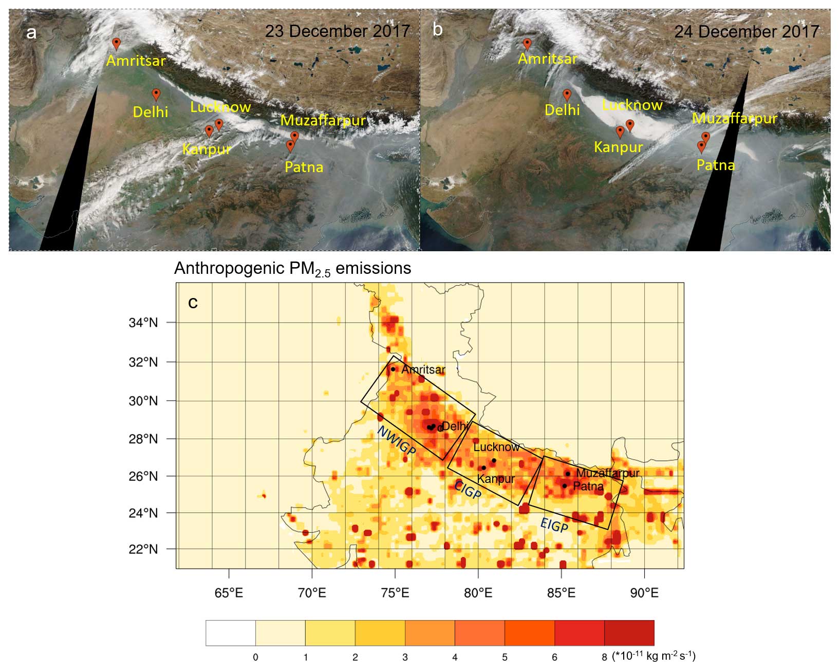
Figure 1The MODIS reflectance (true color) map, representing low cloud over the Indo-Gangetic Plain, India (study region), indicative of likely fog and haze on 23 December (a) and 24 December (b) 2017. The maps are sourced from NASA Worldview (https://worldview.earthdata.nasa.gov/, last access: 19 April 2024). (c) Anthropogenic emissions of PM2.5 over the IGP for December 2017 obtained from EDGAR–HTAP. The boxes represent the regions northwest IGP (NWIGP), central IGP (CIGP), and east IGP (EIGP).
2.1 Modeling
WRF-Chem version 4.0.3 is used for this study. Earlier studies successfully used WRF-Chem to predict fog (Pithani et al., 2019) and in the study of aerosol–radiation feedback on air quality (Kumar et al., 2020; Bharali et al., 2019) and fog (Shao et al., 2023). The model domain is centered at Delhi (28.7° N, 77.1° E) with 300 grid points in the east–west direction, 170 grid points in the south–north direction (Fig. 1c), and 50 vertical eta levels with the model top at 50 hPa. The horizontal grid spacing of the domain is 10 km, while the vertical grid spacing varies from higher resolution (∼ 200 m) in the boundary layer to coarser resolution (∼ 1200 m) near the model top. We conduct three model configurations (Table 1) for 20–24 December 2017 to identify the best configuration for meteorological simulations. The three experiments have been designed with different combinations of meteorological initial/lateral boundary conditions and planetary boundary layer (PBL) physics. Experiment 1 (EXP1) uses the National Centers for Environmental Predictions (NCEP) Final Analysis (GFS-FNL; 1° × 1°, 6-hourly) meteorology data for initial and boundary conditions and the YSU (Yonsei University; Hong et al., 2006) PBL scheme. Experiments 2 and 3 (EXP2 and EXP3) use ERA-Interim Project (1.125° × 0.703°, 6-hourly) for meteorology initial and boundary conditions. EXP2 uses the YSU PBL scheme, while EXP3 uses the ACM2 (Asymmetric Convective Model version 2) PBL scheme. ACM2 is a hybrid of the original non-local closure (Pleim and Chang, 1992) and a local closure eddy diffusion scheme (Pleim, 2007a, b). The YSU PBL option was coupled with the Noah LSM, while ACM2 was coupled with the Pleim–Xiu LSM. While YSU permits investigations of both aerosol–radiation (AR) and aerosol–cloud interactions (ACIs), ACI is not possible when using the ACM2 PBL scheme because in WRF the ACM2 PBL scheme does not provide the exchange coefficient for heat, which is required to calculate the maximum supersaturations and therefore the activation fraction for aerosol mass and number for each bin/mode, which is based on the Abdul-Razzak and Ghan (2002) scheme. However, ACM2 has been shown to perform well for air quality in the polluted regions (Mohan and Gupta, 2018; Gunwani and Mohan, 2017; Xie et al., 2012; Mohan and Bhati, 2011). Mohan and Gupta (2018) tested the YSU and ACM2 schemes during the summertime (1–15 June 2010) and focused on the evaluation of temperature, wind speed, PBL height, ozone, and PM10. Although these studies recommend using the non-local ACM2 PBL scheme for air quality prediction for the IGP, there are still seasonal, day–night, and regional biases in the PBL schemes. Gunwani and Mohan (2017) showed that ACM2, QNSE (quasi-normal scale elimination), and MYJ (Mellor–Yamada–Janjić) schemes work well in predicting temperature, humidity, and wind speed in different regions of India. Mohan and Bhati (2011) found that using the ACM2 PBL scheme with Pleim–Xiu surface physics improved wintertime meteorology estimates in Delhi, indicating its potential in fog predictions, whereas Pithani et al. (2019) recommend using the local PBL scheme MYNN2.5 (Mellor–Yamada–Nakanishi–Niino level 2.5). Shin and Hong (2011) found that a non-local scheme (e.g., ACM2, YSU) is favorable in unstable conditions and that a local scheme (e.g., MYJ, Boulac) is favorable in stable conditions. All these studies suggest the need for careful consideration of the abovementioned biases while selecting a PBL scheme. Therefore, to ensure that WRF captures all the relevant meteorological parameters including relative humidity (RH) reasonably well during fog events in winter, we designed EXP1, EXP2, and EXP3.
Table 1Experiment setup for the study. Numbers in parentheses for the physics options denote the namelist settings of the WRF-Chem model.
The advantage of the Pleim–Xiu LSM (PX-LSM) is that it allows nudging of soil moisture and temperature to improve the prediction of meteorology near the surface (Pleim and Gilliam, 2009; Pleim and Xiu, 2003; Xiu and Pleim, 2001), which the Noah LSM does not include. The PX-LSM includes a two-layer soil model (0–1 and 1–100 cm), canopy moisture, and aerodynamic and stomatal resistance. Ground surface (1 cm) temperature is calculated from the surface energy balance using a force-restore algorithm for heat exchange within the soil. Although the two-layer approach in the PX-LSM is less detailed than the multilayer soil models such as the Noah LSM (four soil layers; Chen and Dudhia, 2001), it performs well with realistic initialization for soil moisture and through dynamic adjustment in the model simulation where soil moisture is indirectly nudged according to differences in 2 m temperature (T2 m) and 2 m relative humidity (RH2 m) between the model and observation (Pleim and Xiu, 2003). Soil moisture nudging adjusts the surface evaporation (direct soil surface evaporation, vegetative evapotranspiration, and evaporation from wet canopies) which then affects the partitioning of available surface energy into latent and sensible heat flux and thus reduces errors in T2 m and RH2 m.
For EXP2, meteorological initial conditions were refreshed every 24 h, while EXP3 was a continuous run, but soil moisture was nudged to the ERA-Interim dataset to improve the prediction of surface fluxes. All other physics and chemistry options are the same for all the experiments except the surface physics option, which changes with the PBL scheme used. The deposition of cloud droplets is an important moisture and aerosol sink during fog events. For all these simulations, the deposition velocity of cloud droplets was reduced to 0.01 m s−1 based on Stokes' law and previous studies (Katata et al., 2015; Tav et al., 2018) because its default value (0.1 m s−1) is large.
To examine the radiative effects of aerosols and aqueous-phase chemistry, additional simulations were done using the meteorological configuration in EXP3, with aerosol–radiation (wFB) feedback plus aqueous chemistry (wAq.chem), without aerosol–radiation feedback (nFB) but with aqueous chemistry, and without aqueous chemistry (noAq.chem) but with aerosol–radiation feedback. The analysis was done for the fog events on 23 and 24 December 2017 as
where FARF is the impact due to aerosol–radiation feedback on the meteorological parameters/chemical species (P) and FAq.chem is the impact due to the inclusion of aqueous-phase chemistry.
Emissions used in the WRF-Chem simulations are from the EDGAR–HTAP v2 (Emissions Database for Global Atmospheric Research–Hemispheric Transport of Air Pollution; 0.1° x 0.1°) inventory for anthropogenic emissions and FINN v2.2 (Fire INventory from NCAR; 1 km x 1 km) fire emission inventory (Wiedinmyer et al., 2011). Trash-burning emissions (Chaudhary et al., 2021) are also included in the simulations. The model calculates the biogenic emissions online using MEGAN v2.04 (Model of Emissions of Gases and Aerosols from Nature) (Guenther et al., 2006). The initial and lateral boundary conditions for chemical constituents are from the global chemistry transport model, CAM-Chem (Community Atmosphere Model with Chemistry) (Emmons et al., 2020).
The MOZART (Model for OZone and Related chemical Tracers) chemical mechanism (Emmons et al., 2010) is used for gas-phase chemistry, which includes 85 gas-phase species, 39 photolysis, and 157 gas-phase reactions. It has been updated to include an explicit treatment of aromatic compounds, HONO, C2H2, and isoprene oxidation scheme (Knote et al., 2014). The lumped toluene used by Emmons et al. (2010) has been speciated into benzene, toluene, and lumped isomers of xylenes (Knote et al., 2014). For this study, HCl emissions, transport, and dry and wet deposition are represented. However, HCl gas-phase reaction is not included in MOZART.
The Model for Simulating Aerosol Interactions and Chemistry (MOSAIC) with four size bins (0.039–0.156, 0.156–0.625, 0.625–2.500, and 2.5–10.0 µm dry diameters) coupled with MOZART gas-phase chemistry is used (Fast et al., 2006; Zaveri et al., 2008). The bin sizes are defined by their lower and upper dry particle diameters, so there is no transfer of particles between bins during water uptake or loss. It is assumed that aerosols in each bin are internally mixed with the same chemical composition, while they are externally mixed in different bins.
The aerosol composition includes sulfate (SO), ammonium (NH), nitrate (NO), aerosol water, sea salt (Na+, Cl−), methanesulfonate (CH3SO3), carbonate (CO), calcium (Ca+), black carbon (BC), organic mass (OC), and unspecified inorganic species such as silica, inert minerals, and trace metals lumped together as other inorganic mass (OIN). For OC, primary OC and secondary OC are represented separately, where the latter is simulated using the volatility basis set (VBS) approach. Reactive inorganic species such as potassium (K+) and magnesium (Mg+) are usually present in much smaller amounts and are equivalent to Na+ since their sulfate, nitrate, and chloride salts are similar in terms of their solubility in water.
MOSAIC treats condensation and evaporation of trace gases to/from particles, nucleation (new particle formation), and coagulation. Aerosol coagulation (Brownian) is based on Jacobson et al. (1994), and nucleation is based on the parameterization of H2SO4–H2O homogeneous nucleation by Wexler et al. (1994). Sulfate, nitrate, chloride, and ammonium aerosols are mainly formed through oxidation and neutralization/condensation of gas precursors. Gas-phase sulfuric acid (H2SO4) is produced by the gas-phase oxidation of SO2 by OH, and nitric acid (HNO3) formation is via the oxidation of NO2 by OH. HCl is a primary emission product. The neutralization/condensation of H2SO4, HCl, and HNO3 with NH3 produces ammonium, such as ammonium sulfate ((NH4)2SO4), ammonium bisulfate (NH4HSO4), ammonium chloride (NH4Cl), and ammonium nitrate (NH4NO3), respectively. The thermodynamic modules in MOSAIC for the dynamic gas–particle partitioning of aerosols MTEM (Multicomponent Taylor Expansion Method) and MESA (Multicomponent Equilibrium Solver for Aerosols) calculate the activity coefficient in aqueous-phase aerosols and compute the intraparticle solid–liquid-phase equilibrium, respectively (Zaveri et al., 2005, 2008). The Adaptive Step Time-split Euler Method (ASTEM) coupled with MESA–MTEM dynamically integrates the mass transfer equations.
Aqueous-phase chemistry uses a bulk water approach employing the Fahey and Pandis (2001) mechanism. It calculates sulfate formation, formaldehyde oxidation, and non-reactive uptake of nitric acid, hydrochloric acid, ammonia, and other trace gases (Chapman et al., 2009; Pye et al., 2020). Aqueous-phase sulfate is produced via oxidation of SO2 by H2O2, O3, TMIs (transition metal ions: Fe(III) and Mn(II)), catalyzed O2, and NO2. TMI concentrations are prescribed in the model to 0.01 µg m−3 for Fe(III) and 0.005 µg m−3 for Mn(II) (Martin and Good, 1991). The Fe(III) values are within the range of water-soluble iron in wintertime aerosols reported in India (Kumar and Sarin, 2010). Wet removal (scavenging) is represented by the Neu and Prather (2012) scheme for trace gases and by Easter et al. (2004) for aerosols.
2.2 Observations
To evaluate the model output, observations of aerosols and meteorology have been obtained from several satellites and ground-based measurement platforms. To examine the aerosol loading and the spatial and temporal distribution, daily Level 2 aerosol optical depth (AOD) retrievals from the Moderate Resolution Imaging Spectroradiometer (MODIS) aboard the Terra and Aqua satellites are obtained at the spatial resolution of 10 km × 10 km (at nadir) pixel array. It provides aerosol properties from the Dark Target (DT) algorithm applied over the ocean and dark land (e.g., vegetation) and from Deep Blue (DB) algorithms over the entire land areas, including both dark and bright surfaces. Each MOD04_L2 (Terra)/MYD04_L2 (Aqua) product is available at a 5 min time interval with an output grid of 135 px in width by 203 px in length.
The Indian National Satellite System (INSAT-3D) in the geostationary orbit at inclinations of 82° longitude provides an imager fog product (3DIMG_L2C_FOG) with a spatial resolution of 4 km every 30 min (https://www.mosdac.gov.in/, last access: 23 December 2021). For daytime, the visible channel observation is used to detect fog, whereas thermal infrared is used to reduce false alarms such as medium/high clouds and snow areas. INSAT-3D's “day microphysics” data component analyzes solar reflectance at three wavelengths: 0.5 µm (visible), 1.6 µm (shortwave infrared), and 10.8 µm (thermal infrared). Nighttime fog is derived from TIR-1 (12.0 and 10.0 µm) and MIR (10.8 and 3.9 µm) channel brightness temperature over the Indian region. INSAT-3D provides fog intensity varying from 1 to 4, indicating SHALLOW for visibility > 600 m and MODERATE, DENSE, and VERY_DENSE, respectively, for visibility varying from 0 to 500 m (Banerjee and Padmakumari, 2020). If the visibility is greater than 700 m it indicates no fog, while visibility > 1000 m represents very clear skies. Validation of INSAT-3D fog products over the IGP shows a 66 %–68 % probability of detection and a 10 % false alarm rate. It also captures the entire life cycle of fog from formation to dissipation. However, detecting fog during multilayer clouds is still challenging with INSAT-3D (Arun et al., 2018; Chaurasia and Gohil, 2015; Chaurasia and Jenamani, 2017).
Ground-based monitoring sites provide hourly data of relative humidity, surface temperature, and wind speed measured by the Central Pollution Control Board (CPCB; https://cpcb.nic.in/, last access: 27 March 2024). Given the data availability from CPCB stations, nine stations have been considered, representing each region of the IGP: Amritsar, IGI Airport (Indira Gandhi International Airport, Delhi), IHBAS (Institute of Human Behaviour and Allied Sciences, Delhi), Dwarka (Delhi), and RKP (Ramakrishna Puram, Delhi) in the northwest IGP; Kanpur and Lucknow in the central IGP; and Patna and Muzaffarpur in the east IGP.
In addition, measurements of several aerosols, trace gases, and meteorology at Delhi (IGI Airport) from the Winter Fog Experiment (WiFEX) for the period 10–31 December 2017 have also been used to validate the model output. The WiFEX, an initiative of the Ministry of Earth Sciences (MoES), India, is a ground-based measurement campaign at the IGI Airport, Delhi, to understand the physical and chemical features of fog. Additional details of the WiFEX and related publications can be found in Ghude et al. (2017).
Previous studies simulating fog highlight the importance of high model vertical resolution (Pithani et al., 2019; Van Der Velde et al., 2010) for representing the fog formation and the growth of the fog layer, model initialization (Yadav et al., 2022), initial relative humidity (Bergot and Guedalia, 1994; Pithani et al., 2020), and PBL schemes (Chen et al., 2020; Pithani et al., 2019). In the present study, 2 m relative humidity (RH2 m), 2 m temperature (T2 m), and 10 m wind speed (WS) from WRF-Chem have been evaluated using ground-based measurements from the CPCB monitoring network and WiFEX campaign for nine stations across the IGP. The comparison of WRF-Chem results with observations shows that RH2 m and T2 m are sensitive to the choice of the meteorological initial and boundary conditions as illustrated by six stations in major cities (Fig. S1 in the Supplement). WRF-Chem compares better with the observations for simulations driven by the ERA-Interim reanalysis than with GFS-FNL reanalysis, since ERA-Interim provides more realistic RH2 m than GFS-FNL (Fig. S2a–f). For example, RH2 m from EXP1 (GFS) varies from 10 % to 50 %, while RH2 m from EXP2 and EXP3 varies from 30 % to 100 %, which is closer to observation, especially for the NWIGP and CIGP. For the EIGP, RH2 m from EXP1 (GFS) compares better than ERA-Interim, which overestimates the observed RH2 m. ERA-Interim and the YSU PBL scheme showed damping of RH2 m continuously increasing the bias in RH2 m with time (not shown), which was corrected in EXP2 by refreshing meteorology every day at 00:00 UT during the model simulation. In addition, maps of surface RH2 m and T2 m (Fig. S2g–j) show that the GFS-FNL dataset has lower relative humidity throughout the domain as compared to ERA-Interim. There are differences in simulated 2 m temperature between these two datasets which are of smaller relative magnitude compared to the RH2 m.
The GFS-FNL-driven meteorology EXP1 has a warm bias in the NWIGP and CIGP, especially during the nighttime, while over the EIGP, the model prediction agrees well with observations. EXP2 with the ERA-Interim-driven meteorology and YSU PBL scheme also shows good agreement between modeled and observed T2 m in the EIGP. The ERA-Interim-driven meteorology with the ACM2 PBL scheme in EXP3 has a cold bias of up to 7 °C over the EIGP during the daytime from 22 to 24 December. The wind speed evaluation shows that WRF-Chem is over-predicting wind speed. However, it is also possible that some CPCB stations (e.g., Amritsar and RK Puram) have a low wind speed bias due to the low measurement height and obstructions such as tall trees near the monitoring station, as shown in Fig. S3. WRF-Chem in general overestimates wind speed, and several earlier studies have reported this bias in wind speed (e.g., Mohan and Gupta, 2018; Pithani et al., 2019). Moreover, WRF-Chem does not have the capability to represent building meteorology and parameterizes the effects of urban areas on meteorology through roughness length, which likely leads to overestimation of wind speed. Note that at other sites (e.g., over IGI Delhi and Kanpur) the model measurement agreement is better.
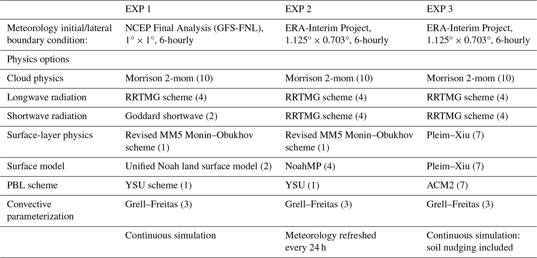
The WRF-Chem performance has been statistically assessed against observations using the Taylor diagram (Taylor, 2001), which provides a statistical summary of how well the model output agrees with the observation in terms of the Pearson correlation, their centered root-mean-square error (RMSE) difference, and the ratios of their variances (Fig. 2). The centered RMS difference is proportional to the distance to point “OBS” in the x axis which measures the extent to which the simulated and observed datasets match. The centered RMS difference (E′); the correlation (R); and the standard deviations, (simulated) and (observed), are calculated as
where the overall mean of a field is indicated by an overbar.
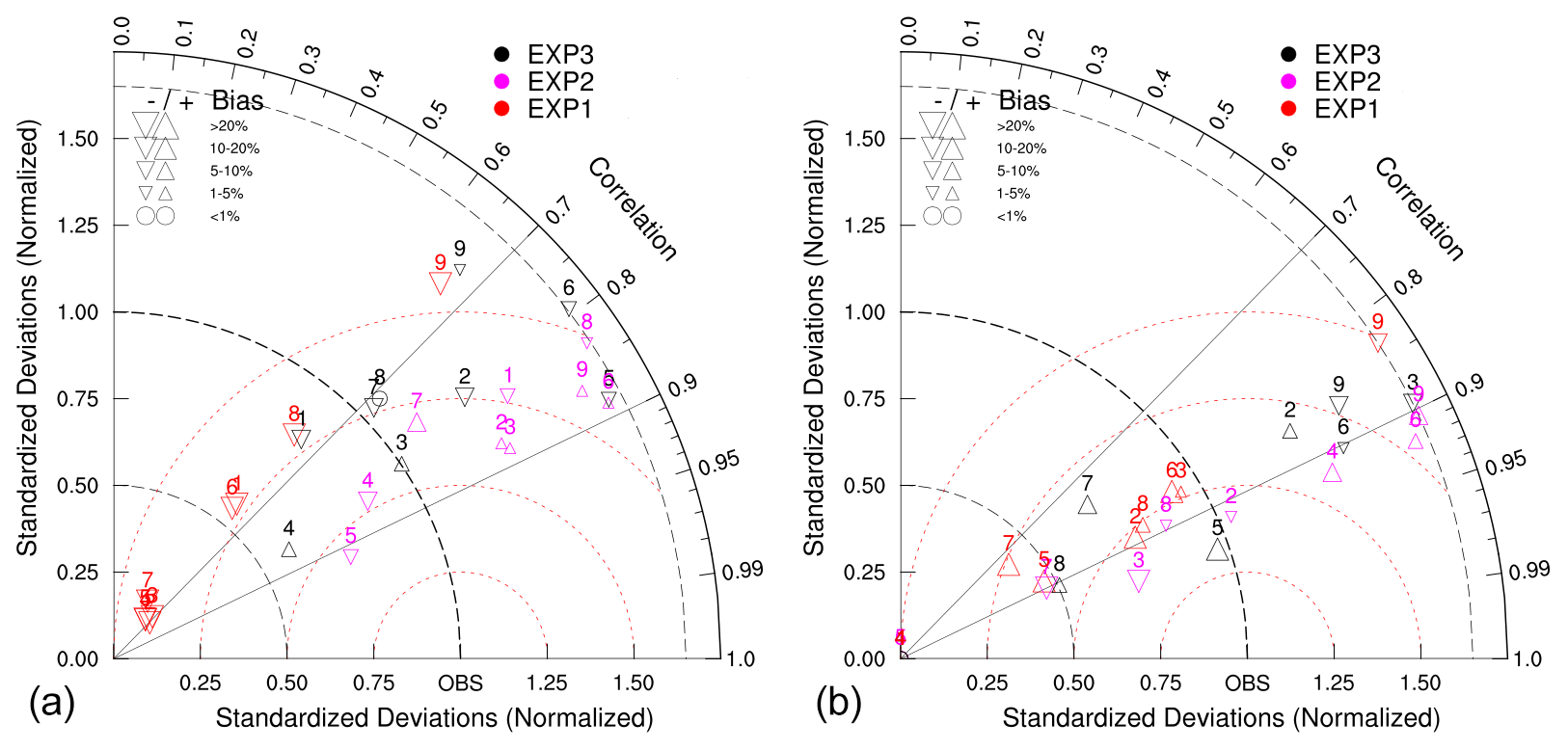
Figure 2Taylor diagram of simulated (WRF-Chem) and observed (CPCB) relative humidity (a) and 2 m temperature (b) over the IGP. The colors indicate the experiments. The dotted red contours represent RMS values. The marker (triangles) size varies with a mean bias between the experiments and observations. Upside-down triangles represent positive bias (exp-obs) and vice versa. The stations over the IGP are denoted by number. 1: Amritsar. 2: IGI Airport (Delhi). 3: IHBAS (Delhi). 4: Dwarka (Delhi). 5: RKP (Delhi). 6: Kanpur. 7: Lucknow. 8: Patna. 9: Muzaffarpur. The locations are marked in Fig. 1a.
Each point in the two-dimensional space of the Taylor diagram represents the abovementioned three different statistical metrics simultaneously, as they are related by the following equation:
The diagram is constructed based on the similarity of the above equation and the law of cosines:
The percentage bias has also been included to further evaluate the WRF-Chem results. In Fig. 2, better agreement of WRF-Chem results with observations is shown by the marker's proximity to the “OBS” dashed black line. The WRF-Chem RH has a good correlation for all three experiments with r > 0.75 at all the locations in the IGP for all the experiments. However, the RMSE (shown by dashed red contours) and the standard deviations are larger for EXP1 compared to EXP2 and EXP3, which lie closer to the dashed black line, indicating that the simulated RH2 m variations are similar to observations. The mean bias is also large (> 20 %) for EXP1 (GFS-FNL) for all the stations, marked by red triangles. For example, simulated RH2 m at Dwarka (4) and Lucknow (7) for EXP2 and IGI Airport (2), IHBAS (3), Lucknow (7), and Patna (8) for EXP3 show good agreement with observations, with r > 0.7, the standard deviation within ±0.25, and the mean bias within 10 %. Among these stations, the model performs better for Dwarka (4) and Lucknow (7) for EXP2 and for IGI Airport (2) and IHBAS (3) for EXP3 with a smaller centered RMSE (< 0.75).
For all the experiments, WRF-Chem T2 m agrees well with observations with a correlation between 0.8 and 0.95. The points are concentrated near the dashed line, showing a low RMSE and standard deviation for T2 m, signifying a good agreement of simulated T2 m with observations in terms of temporal variation, but the T2 m relative bias is large for EXP1 (> 20 %). The RMSE and relative bias for EXP1 are larger for several of the stations. For example, simulated T2 m agrees best with observations at IHBAS (3) for EXP1 and IGI Airport (2) for EXP2, with smaller centered RMSE and standard deviation and with bias < 5 %. The temporal variability in T2 m and RH2 m is predicted well for all the combinations of inputs (Fig. S1); however, the accuracy of simulated T2 m and RH2 m is sensitive to the choice of meteorological initial/boundary conditions. WRF-Chem predicted that RH2 m and T2 m agree better with observations when initialized with ERA-Interim meteorology than with GFS-FNL.
The WRF-Chem runs driven by ERA-Interim with the YSU (EXP2) and ACM2 PBL (EXP3) schemes predicted the surface meteorology better over the IGP than the WRF-Chem run driven by GFS (EXP1). By examining the modeled cloud water content (averaged over all the grids in the analysis region) in the lowest model level with the INSAT-3D satellite fog intensity for 23 and 24 December 2017 (Fig. 3), it is apparent that WRF-Chem with the ACM2 PBL scheme compared qualitatively well with observations obtained from the INSAT-3D satellite in terms of fog coverage over the CIGP, while the WRF-Chem run with the YSU PBL scheme did not produce widespread fog. However, there is also fog over the EIGP in WRF-Chem with the ACM2 PBL scheme, although it is not observed by the satellite. This is because the model has a cold bias in T2 m and a high RH2 m over the east IGP with ACM2 PBL and the Pleim–Xiu surface scheme, as discussed earlier, which favors the formation of fog in this region. The time series in Fig. 4 shows that EXP3 is capable of predicting the duration of fog on 23 and 24 December. There is a data gap from INSAT-3D observations because the satellite is unable to capture fog during the daytime in the presence of mid- and high-level clouds. Although fog liquid water content (LWC) data are available for Delhi from the WiFEX campaign, the WRF-Chem simulation does not produce fog in the NWIGP; therefore, the WiFEX observations are not included in this evaluation.
Figure 3Average WRF-Chem surface-layer cloud water mixing ratios (g m−3) for EXP2 and EXP3 (a, b, c, d) and INSAT-3D satellite fog intensity (e, f) on 23 and 24 December 2017. INSAT-3D satellite fog intensity varies from 0 to 4 indicating SHALLOW, MODERATE, DENSE, and VERY_DENSE, respectively. The rectangle in the central IGP is the region for the time series analysis.
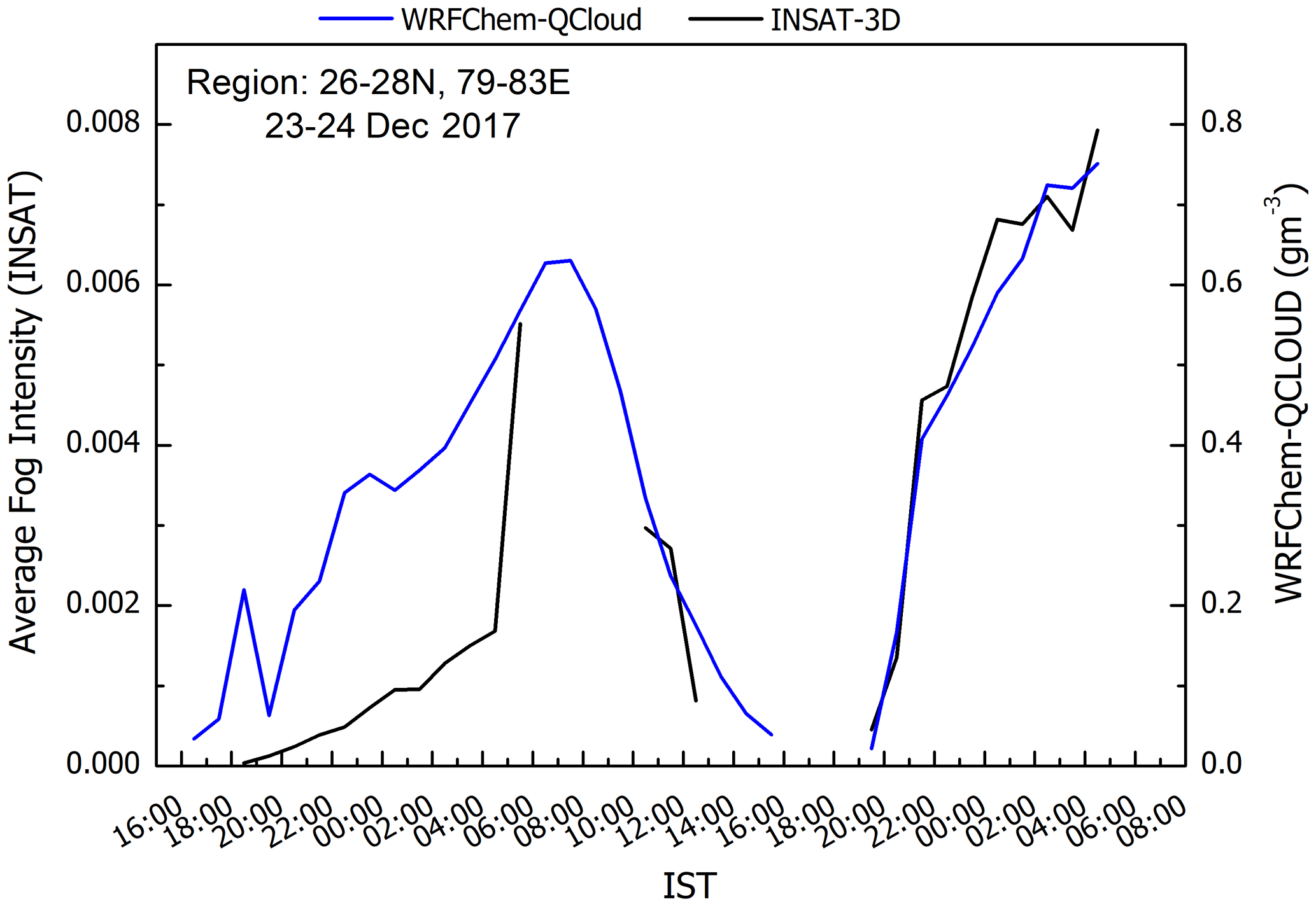
Figure 4Average hourly variation in fog on 23 and 24 December 2017 from the WRF-Chem EXP3 simulation and the INSAT-3D satellite between 26–28° N and 79–83° E (region shown in Fig. 3). The time is in IST (Indian Standard Time; IST is 5.5 h ahead of Coordinated Universal Time (UTC)).
In conclusion, EXP3 is the best configuration for predicting fog formation where the ERA-Interim meteorology, the ACM2 PBL and surface schemes, and soil moisture nudging are used in the WRF-Chem simulation. Therefore, the evaluation of predicting AOD, surface aerosol concentrations, and aerosol composition, as well as analysis of the impact of aerosols on fog formation, uses the EXP3 configuration.
Aerosols are an important factor in the correct prediction of fog (Maalick et al., 2016; Stolaki et al., 2015) as the number of fog droplets depends on the aerosol size distribution and concentration. Aerosols as CCN can affect the liquid water content in fog; therefore, an increase in aerosol concentration can significantly affect fog lifetime (Stolaki et al., 2015; X. Zhang et al., 2014). AOD retrievals from the MODIS satellite have been used to validate the modeled AOD (Fig. 5). It is observed that the model captures several important features of the MODIS-retrieved AOD spatial distribution but at the same time somewhat struggles to reproduce the observed AOD magnitude in some parts of the domain. One possible reason for the underestimation would be the EDGAR–HTAP emission inventory, which has a low bias for residential-sector PM2.5 emissions in India (Sharma et al., 2022). For instance, the model successfully predicts high aerosol loading seen by MODIS on 20 and 21 December over the CIGP and EIGP. This is the region with dense fog both in the model and the observations. Higher AOD (> 0.5) over the CIGP and EIGP can be attributed to the accumulation of aerosols that are transported by northwesterly winds to these regions from the NWIGP (Dey and Di Girolamo, 2011; Jain et al., 2020; Jethva et al., 2018; Kumar et al., 2018; Yadav et al., 2020). However, WRF-Chem underestimates AOD over the NWIGP (AOD < 0.3) throughout the simulation period and during 23–24 December over the CIGP and EIGP, where the latter may be related to enhanced scavenging of aerosols by fog droplets.
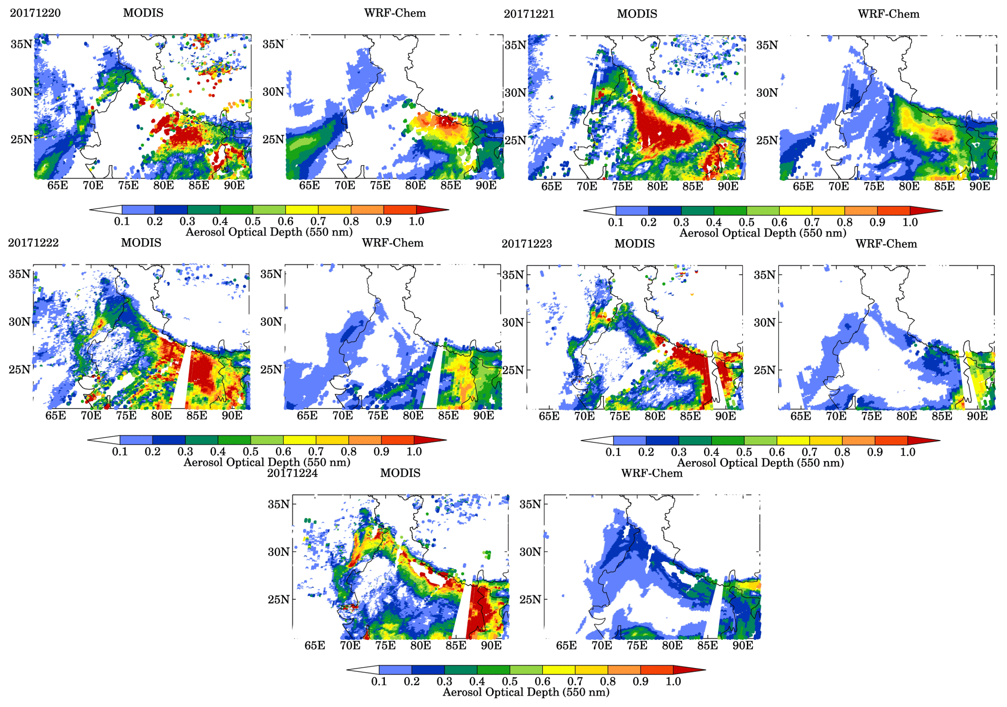
Figure 5Comparison of WRF-Chem AOD with MODIS observations over the model domain on 20, 21, 22, 23, and 24 December 2017.
The west-to-east gradient in aerosol loading over the IGP is consistent with surface PM2.5 distribution (Fig. 6a). Surface PM2.5 concentration is highest in the EIGP (> 100 µg m−3), and it decreases gradually towards the NWIGP (∼ 60–80 µg m−3). The time series of PM2.5 from CPCB measurements and the model at stations representative of each region in the IGP show that simulated PM2.5 compares well with observations in terms of day-to-day variation over most of the locations in the IGP (Fig. 6b–e). The comparison is good over Amritsar (an NWIGP location), where PM2.5 is mostly primary aerosols from local emissions, e.g., residential-heating-related biomass burning. Agricultural waste burning is at its peak during post-monsoon months (October–November), whereas, during winter, burning for residential heating increases, and the stable boundary layer confines these emissions near the surface (Kumar et al., 2021; Pawar and Sinha, 2022). PM2.5 at Amritsar shows a bimodal distribution with morning and evening peaks, whereas it is absent in the model, likely due to the absence of diurnal variations in the WRF-Chem anthropogenic emissions.
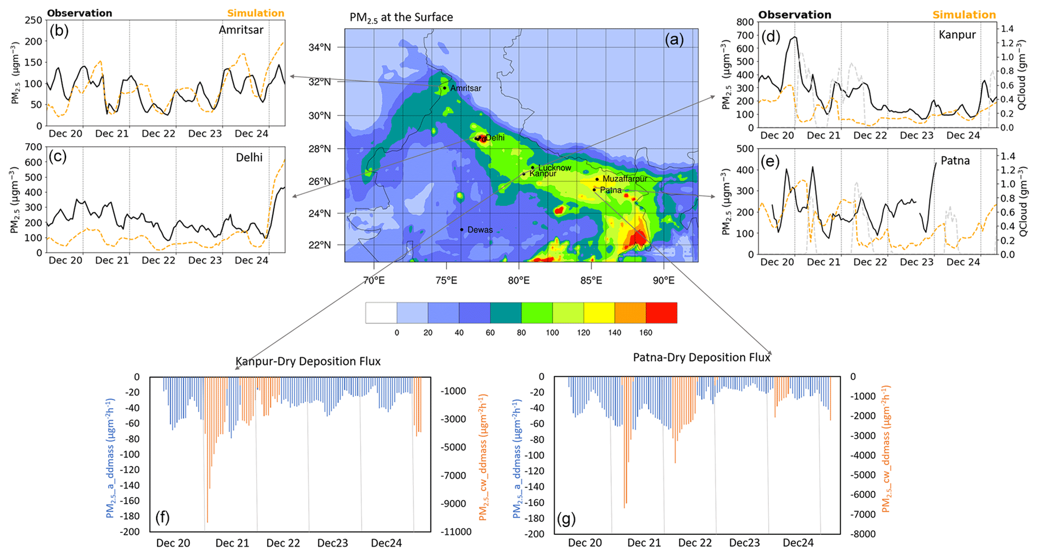
Figure 6WRF-Chem-simulated surface PM2.5 map over the IGP (a). Comparison of WRF-Chem PM2.5 with CPCB observation for the period 20–24 December 2017 for (b) Amritsar, (c) Delhi, (d) Kanpur, and (e) Patna. Dry deposition rate of PM2.5 for (f) Kanpur and (g) Patna. The dotted gray line in (d) Kanpur and (e) Patna is fog (QCloud) present during the study period.
At Delhi, the daily variations are predicted well, although WRF-Chem underestimates PM2.5 observations during the first 4 d. Delhi experiences severe air pollution and haze with high PM loading (> 500 µg m−3) (Bharali et al., 2019). The model is successful in predicting the high-PM2.5 episode on 24 December, but WRF-Chem underpredicts the SO, NH, NO, and Cl− concentrations (Fig. 7). Although simulated SO2 and NH3 are comparable with the observations, sulfate and ammonium are underestimated in the model. SO is underestimated by ∼ 9 µg m−3, while NH, NO, and Cl− are underestimated by ∼ 30, ∼ 19, and ∼ 40 µg m−3 on average, respectively. In addition, the WRF-Chem model results show that a large percentage of PM2.5 is classified as “other inorganics”, which is usually dominated by PM2.5 other than BC and OC. The WiFEX observations show that secondary aerosols contribute ∼ 50 % of the PM2.5 concentration, which is in line with other studies which found that secondary aerosols contribute 15 %–50 % to PM2.5 mass (Sharma and Mandal, 2017; Behera and Sharma, 2010; Nagar et al., 2017) and that NO constitutes 9 %–13 % of PM2.5 mass (Lalchandani et al., 2021; Sharma and Mandal, 2017). This leads to the underestimation of PM2.5 over Delhi. Studies report very high chloride over the IGP, with values exceeding 100 µg m−3 (Lalchandani et al., 2021) during winter from increased trash-burning and industrial emissions (Pant et al., 2015; Patil et al., 2013). WRF-Chem incorporates trash-burning emissions which include HCl emissions from Chaudhury et al. (2021) for this study; however, the inventory contains annual emissions and fails to resolve the seasonality of trash-burning emissions as identified by Nagpure et al. (2015). They suggested that almost all the waste-burning emissions in neighborhoods with higher socioeconomic status in Delhi occur due to the use of waste as cheap heating fuel by individuals such as night guards and pavement dwellers. Chaudhary et al. (2021) considers waste burning that occurs due to the lack of collection infrastructure and landfills, showing a concentration of waste-burning emissions around the periphery of Delhi but low waste-burning emissions in the relatively prosperous city center. In addition, emissions from other sources (e.g., industries) are unaccounted for in the model, which likely leads to the underestimation of modeled chloride.
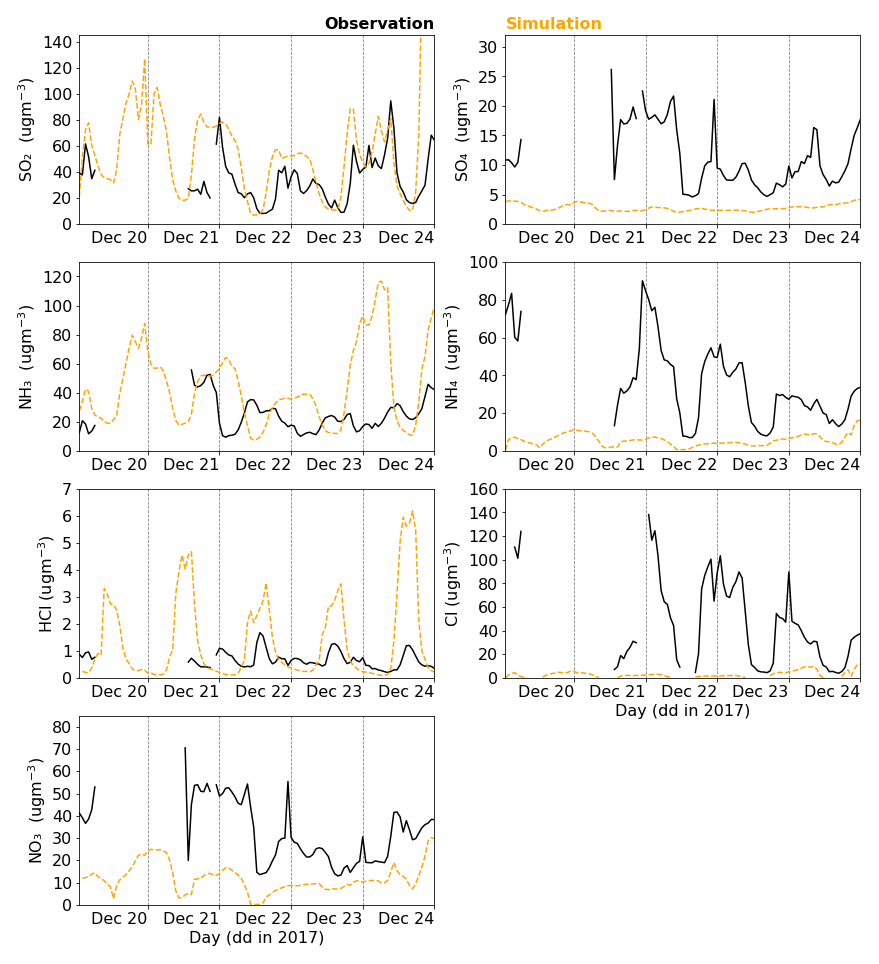
Figure 7Comparison of WRF-Chem-simulated ions (SO, NH, NO, and Cl−) and trace gases (SO2, NH3, and HCl) with the observations from the WiFEX campaign at Delhi.
Over the CIGP and EIGP, the underestimation of PM2.5 is mostly observed during the dense fog. It is well-known that the hygroscopic aerosols grow in size and are deposited to the surface during fog (Gupta and Mandariya, 2013; Kaul et al., 2011). PM2.5 shows an increase initially with the onset of fog, and then it decreases as the aerosols grow and get deposited through fog droplets. A 2-order-higher deposition rate (Fig. 6f, g) during fog compared to the deposition rate of dry aerosols results in the lower PM2.5 over the CIGP and EICP during fog events.
A statistical analysis (Table S1 in the Supplement) shows a minimum normalized mean bias (NMB) for PM2.5 at Amritsar (2.2 %), while in other stations the normalized mean bias ranges from 48 % to 53 %, similar to the reported range of model bias (underestimated by 40 %–60 %) in winter over the IGP by earlier studies (Bran and Srivastava, 2017; Ojha et al., 2020). This was accomplished by incorporating trash-burning emissions in the model simulation, which improved the PM2.5 prediction, increasing the NMB by ∼ 4 %–8 % in the IGP. RMSE values range from 41 to 138 µg m−3 (normalized RMSE ∼ 0.4 to 0.7), comparable to the reported values by these studies. The Pearson correlation coefficient (r) for the simulated and observed day-to-day variation in PM2.5 lies between 0.4 and 0.7 for all the stations in Fig. 6 except at Patna and Muzaffarpur, which lies within the range in these studies. The poor correlation at Patna and Muzaffarpur is due to the low modeled PM2.5 concentrations which are caused by the increased dry deposition of aerosol particles activated as fog droplets during fog periods, as discussed earlier. Furthermore, the fog events in WRF and in the observations have somewhat different time periods, causing the WRF-predicted and observed PM2.5 concentrations to decrease at different times.
Previous studies have reported that models tend to underestimate the AOD observations (David et al., 2018; Pan et al., 2015) during the post-monsoon season and winter when agricultural waste-burning and anthropogenic emissions dominate. While anthropogenic emissions include a contribution from the residential sector, the emissions from small-scale burning for residential heating over the IGP, especially during winter, are likely underestimated in the current emission inventory (Sharma et al., 2022). This leads to an underestimation of aerosol concentration in the model. Other possible causes for the underestimation are the biases in the simulated meteorology (Govardhan et al., 2015; Kumar et al., 2015; Pan et al., 2015) which affect the aerosol concentration. We corrected some of the biases in meteorology as discussed earlier; however, there are still residual biases in the simulated meteorology, e.g., overestimation of wind speed by WRF-Chem. We also observe underestimation of secondary aerosols over the NWIGP which contribute significantly to the aerosol loading over the IGP. Secondary aerosol formation is substantial over the CIGP and EIGP in the model compared to the NWIGP, which will be discussed in a later section. The underestimation of PM2.5 could also be linked to the uncertainty in the model's chemistry scheme to simulate the secondary aerosols due to missing chemical processes or due to the underestimation of sulfur oxidation at different RH levels (Acharja et al., 2022; Pawar et al., 2023; Ruan et al., 2022). Moreover, several modeling studies have shown significant improvements in forecasting surface PM2.5 by the assimilation of satellite AOD and PM2.5 (Ghude et al., 2020; Jena et al., 2020; Kumar et al., 2020), suggesting the importance of correct initialization of the model in simulating aerosols over the IGP.
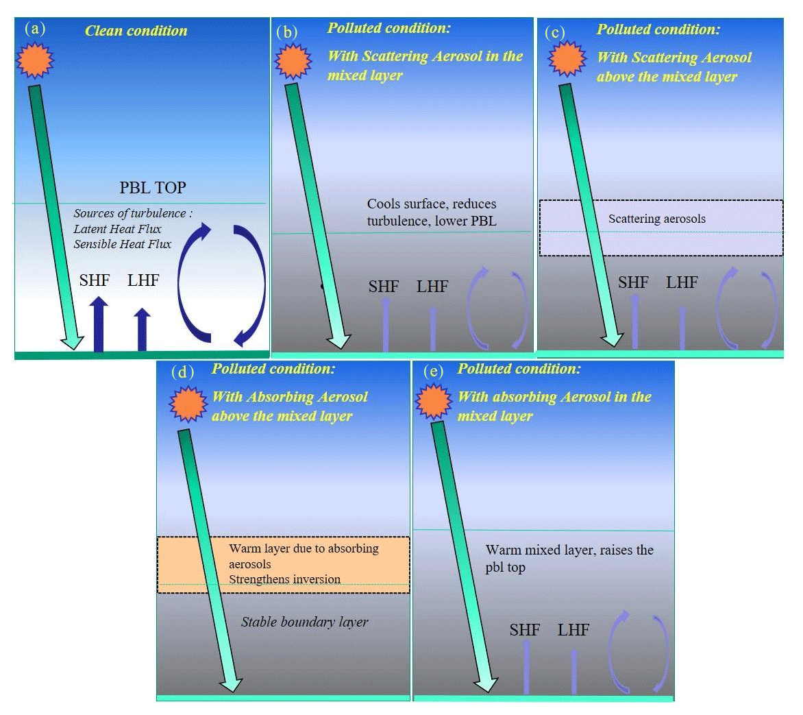
Interactions of aerosols with radiation affect temperature and surface heat fluxes, thereby weakening the turbulence in the PBL and stabilizing the boundary layer height (Fig. 8b) compared to the clean environment (Fig. 8a). In the presence of well-mixed aerosols within the PBL, the radiative effect of aerosols lowers the noontime PBL height (Fig. 8b). However, the presence of absorbing aerosols in the PBL warms the air and changes the thermodynamics. Three cases are shown in Fig. 8c–e, where increases in scattering aerosol concentrations at the top of PBL (Fig. 8c) increase scattering of radiation by the aerosol layer and reduce the surface-reaching solar radiation similar to Fig. 8b. Higher concentrations of absorbing aerosols at the top of the PBL (Fig. 8d) warm the air above the boundary layer and strengthen the capping inversion, stabilizing the PBL and suppressing its growth. The shallow PBL and weakened daytime vertical mixing confine aerosols and water vapor near the surface and worsen the air quality of a region. The aerosols trapped in the stagnant PBL further affect the radiation flux at the surface and create a positive feedback loop wherein the PBL is continually suppressed until interrupted by some synoptic weather phenomenon, such as the western disturbances in the IGP. On the other hand, a higher concentration of absorbing aerosols within the PBL (Fig. 8e) warms the air in the PBL, and this results in the greater PBL height. The raised PBL decreases the aerosol concentration near the surface, which is termed a negative feedback effect.
The aerosol–radiation feedback can affect shortwave heating rates (SWHRs). The high aerosol loading over the IGP (Figs. 6 and 7) allows the AR feedback to reduce the PBL height by more than 140 m throughout the IGP compared to the surrounding region with AR feedback (Fig. 9a). The difference in PBL height with and without aerosol–radiation feedback is largest during noontime. The suppressed PBL is due to the decrease in the surface heating flux and the consequent weakening of turbulence in the PBL. The surface solar radiation flux (SWF) decreases by 5 %–35 %, while the surface latent heat (LH) and sensible heat (HFX) fluxes decrease by 5 %–35 % and 10 %–60 %, respectively (Fig. S3). The stable, shallow PBL reduces the vertical mixing of aerosols and moisture and confines them near the surface, resulting in increased PM2.5 concentrations and RH near the surface with AR feedback (Fig. 9). Although T2 m should decrease with the reduction in surface SWF, T2 m shows mixed signals with both cooling and warming over the IGP. While surface cooling is observed over the NWIGP and EIGP, T2 m increases with AR feedback over most of the CIGP. The response of AR feedback to T2 m varies in these three regions probably due to differences in the distribution and types of aerosols and the presence of fog. An increase in surface concentration of PM2.5 occurs more over the NWIGP and EIGP with an increase in BC and OIN over the NWIGP and an increase in sulfate aerosol over the EIGP, which results in the surface cooling due to positive AR feedback in these two regions. Over the CIGP, the AR feedback causes a depletion of surface PM2.5 (Fig. 9d), which is likely due to hygroscopic growth, and then dry deposition (average PM2.5 dry deposition flux of 331 with AR feedback and 282 without AR feedback) in dense fog. The increase in RH with AR feedback favors the growth of aerosols in size by the uptake of water.
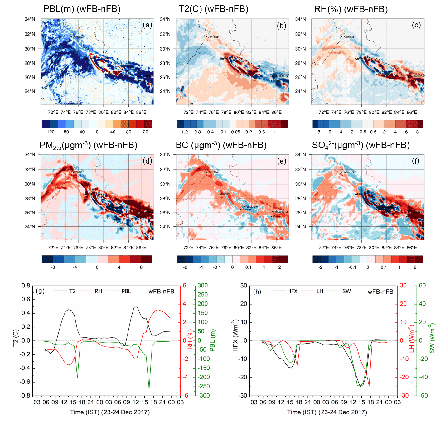
Figure 9Effect of aerosol–radiation feedback (wFB–nFB) on (a) PBL height, (b) 2 m temperature, (c) 2 m relative humidity, (d) surface PM2.5, (e) surface BC, and (f) surface SO4 for 24 December at local noon (13:30–15:30 IST). (g) The time series of ΔPBL, ΔT2, and ΔRH. (h) ΔHFX (sensible heat flux), ΔLH (latent heat flux), and ΔSWF (downward shortwave flux) over the CIGP for 23 and 24 December. Δ denotes the difference between simulations with and without AR feedback (wFB–nFB).
A further examination of the time variation in the changes in PBL height, T2 m, and RH between the simulations with and without aerosol–radiation feedback (Fig. 9g) shows an increase in T2 m, while the surface fluxes, sensible heat flux, latent heat flux, and downward shortwave radiation flux decrease over the CIGP (Fig. 9h). AR feedback affects mostly the lower atmosphere at multiple levels; however, our finding suggests that the decreased shortwave radiation flux decreases the surface fluxes and thus the turbulence in the boundary layer, resulting in a reduced PBL height on both days. Figure 9g and h clearly show a decrease in HFX and LH following the decrease in SWF. Moreover, we observe that the PBL height is sensitive to latent heat flux likely due to its strong dependence on moisture availability (Xiu and Pleim, 2001; Zhang and Anthes, 1982).
The impact of AR feedback on T2 m depends on factors such as the presence of absorbing aerosols and their vertical distribution via heating or increased SWF (as observed in the CIGP; Fig. S4). Absorbing aerosols in WRF-Chem include BC and OIN (other inorganic aerosols), which both increase near the surface (Figs. 9e, S5) due to their confinement in the stable PBL. Some areas in the fog-affected region show a decrease in BC and SO, likely due to increased dry deposition in fog water, as discussed earlier in this section for PM2.5. As a result, AR feedback changes the absorbing-to-scattering ratio of aerosols over the IGP indicated by the decrease in single-scattering albedo (SSA; Fig. S6). In the EIGP, sulfate concentrations are larger with AR feedback than without AR feedback in time periods where the difference is > 1 µg m−3 (Fig. 11). The BC concentration changes are small (< 0.5 µg m−3) in the EIGP, resulting in a higher SSA near the surface with AR feedback in the EIGP. In the CIGP, BC concentrations increase, while sulfate aerosols decrease within the PBL with AR feedback (Fig. 11) compared to the simulation without AR feedback. A decrease in SSA is seen for the CIGP throughout the boundary layer, while in the EIGP the decrease occurs near the top of the PBL; the difference in SSA due to AR feedback is negligible in the NWIGP. Also contributing to the higher SSA in the EIGP is the increase in RH (Fig. 9) due to AR feedback favoring the growth of aerosols in size by the uptake of water and the production of secondary aerosols such as SO and NH.
A similar observation has been made by Ramachandran et al. (2020), where SSA decreases with increasing altitude due to absorbing carbonaceous aerosols at higher elevations, which contributes ≥ 75 % to the aerosol absorption over the IGP. Increased shortwave heating (Fig. 10) is probably caused by the increased absorbing aerosols near the surface, which overwhelms the surface cooling due to reduced shortwave radiation at the surface.
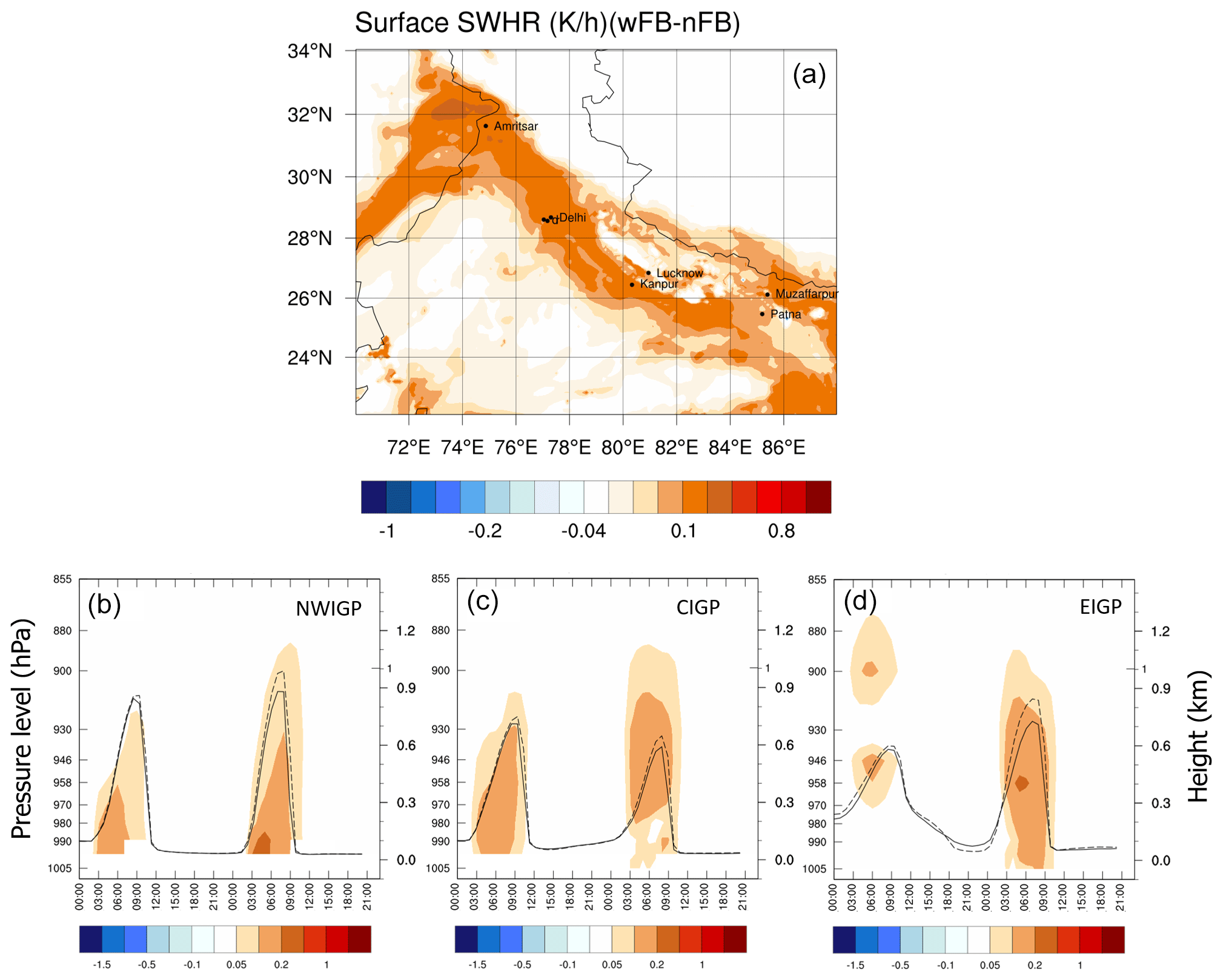
Figure 10Differences in shortwave heating rates (K h−1) between simulations with and without aerosol–radiation feedback (a) at the surface and for pressure–time cross-sections over the (b) NWIGP, (c) CIGP, and (d) EIGP for 23 and 24 December. The solid and dashed lines are the PBL height with and without AR feedback, respectively. The time is in IST.
The increase in 2 m RH is substantial over the CIGP on 24 December (Fig. 9g) compared to the previous day following the decrease in PBL height, which constrains the moisture near the surface. The decrease in RH by 2 % or more when aerosol–radiation feedback is included compared to no aerosol–radiation feedback is likely due to the increase in T2 m. However, the increase in RH in the afternoon associated with a decrease in LH and PBL height is important for the air to saturate, which then favors the formation of fog in a polluted environment. Note that the increase in T2 m with AR feedback is very small (< 0.5 °C), which reduces further after noon (∼ 12:30 IST) on both days.
Another important factor that can affect the extent of change in PBL height is the distribution of aerosols in the vertical (illustrated in Fig. 8). The pressure–time cross-sections of differences in T, PM2.5, BC, and SO between aerosol–radiation (AR) feedback (wFB) and no aerosol–radiation feedback (nFB) for three regions, the NWIGP, CIGP, and EIGP, are shown in Fig. 11. The difference in the PBL height reaches a maximum with the AR feedback during midday (12:30–15:30 IST). An increase in temperature in the boundary layer is observed with AR feedback particularly at the upper PBL in all the regions of the IGP. This induces a temperature inversion resulting in a stable and suppressed PBL. In all the regions the decrease in PBL height (100–200 m) is larger on 24 December compared to 23 December. The difference in the PBL height on 23 and 24 December with AR feedback on these days is possibly controlled by the aerosol distribution during the previous day or early morning on the same day. For example, in all the regions, an increase in PM2.5 is observed the previous night (23:30 IST onwards) until ∼ 11:30 IST of 24 December with increased BC over the NWIGP and CIGP, whereas both BC and SO increased over the EIGP. The increased PM2.5 concentrations suppress the development of the PBL after sunrise with AR feedback on 24 December compared to on 23 December, leading to the observed differences in ΔPBL height on these 2 d. An increase in BC concentrations in the NWIGP and CIGP is found above the PBL on 24 December, whereas BC concentrations decrease within the PBL. This BC concentration gradient creates a temperature inversion, for example between 10:30 and 14:30 IST. The increase in BC warms the air in the PBL; however, the warming is not strong enough to cause negative feedback over the CIGP. On 23 December a small increase in BC is uniform throughout the PBL, while there is a decrease in SO concentrations, resulting in a warmer PBL (Fig. 11) with AR feedback.
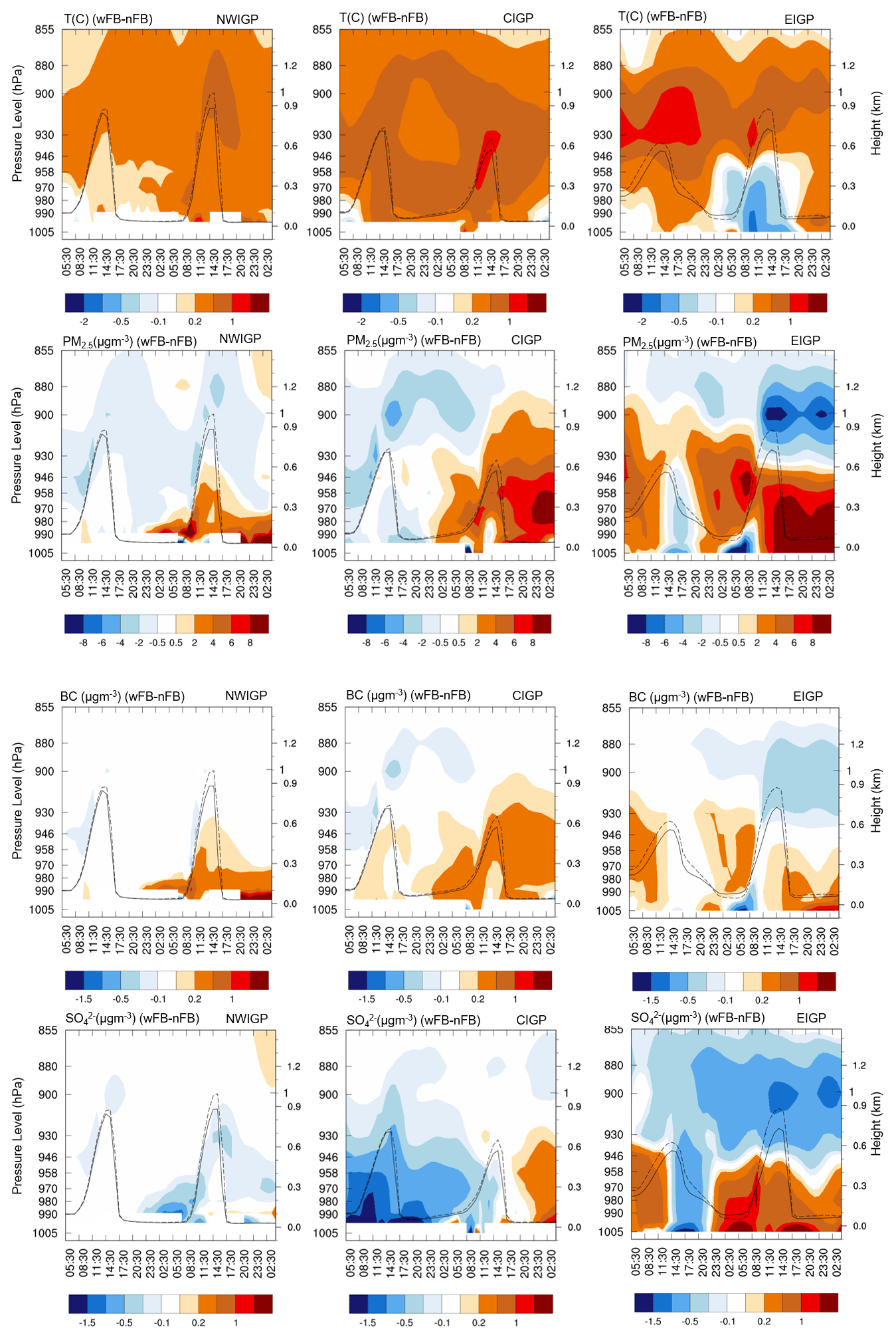
Figure 11Pressure–time cross-section of the differences in T, PM2.5, BC, and SO between simulations with and without the AR feedback for 23 and 24 December. The solid and dashed lines are the PBL height with and without AR feedback, respectively. The time is in IST.
In the EIGP, BC distribution is similar to that in the CIGP with AR feedback, while there is a substantial increase in sulfate aerosols in the PBL. This results in the strongest extinction in the EIGP, as evidenced by the largest difference in PBL height and surface cooling with AR feedback among the three regions. Although ΔPBL is small on 23 December, it still results in the accumulation of aerosols during the nighttime (∼ 23:30 onwards), which further strengthens the AR feedback effect the next day in the NWIGP and CIGP. Thus, AR feedback stabilizes the PBL and increases PM2.5 and RH in the PBL, making conditions favorable for the persistence of fog over the IGP.
In this section we discuss the impact of aqueous-phase chemistry on aerosol composition and its interaction with meteorology. There is a considerable difference in the surface concentration of PM2.5 (> 16 µg m−3) in the absence of aqueous chemistry over the CIGP and EIGP where fog occurs (Fig. 12a), while the difference is negligible over the NWIGP where fog does not occur. This is due to the formation of secondary aerosols through aqueous-phase chemistry and the hygroscopic growth of aerosols during fog in these regions with the inclusion of aqueous chemistry in the model. In the region between the CIGP and EIGP (83–84° E; marked by the box in Fig. 12a), PM2.5 concentration is less in the simulation with aqueous-phase chemistry than without aqueous-phase chemistry because deposition of fog water aerosols to the surface increases as the fog thickens (Figs. 13, S7). Figure 13 shows the relation between the formation of secondary aerosols, deposition flux of PM2.5, and fog with and without aqueous-phase chemistry. During the fog event, the secondary aerosols (SO and NH) increase significantly by 4–10 µg m−3 due to aqueous-phase chemistry adding to the PM2.5 burden over the IGP. The intensity of fog is high around midnight on 24–25 December compared to on 23–24 December (01:30–11:30 IST), which increases the dry deposition flux of PM2.5, causing a sharp drop in the PM2.5 concentration on 24 December compared to the previous night's fog event. The observed change in PM2.5 over a region is the net result of the formation of secondary aerosols and its deposition with fog droplets.
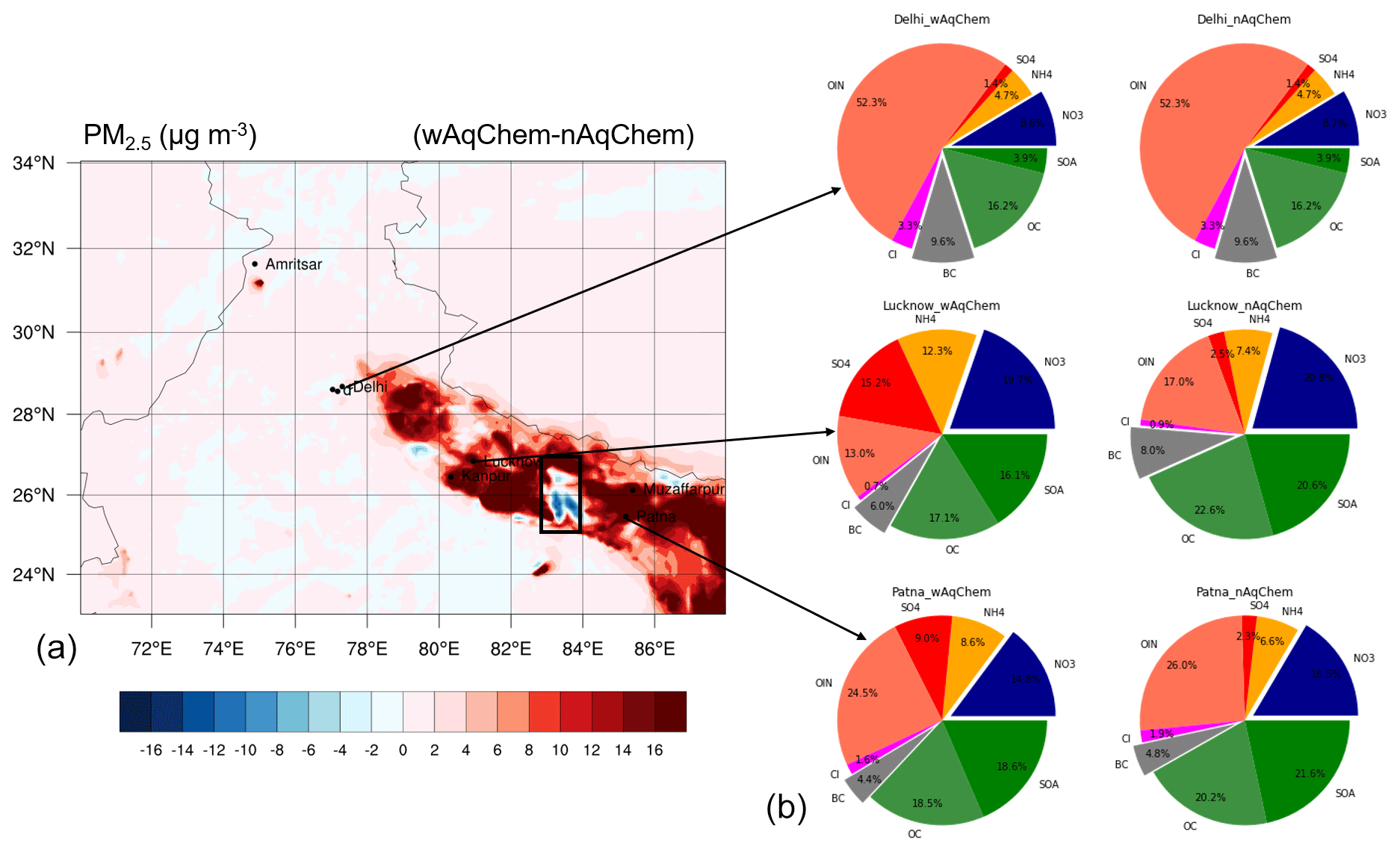
Figure 12Surface ΔPM2.5 (wAq.chem-noAq.chem) (a) and pie charts of PM2.5 composition distribution (b) for the two cases, with and without aqueous-phase chemistry, for 24 December 2017. The stations Delhi, Lucknow (LKN), and Patna are representative of the NWIGP, CIGP, and EIGP regions, respectively.
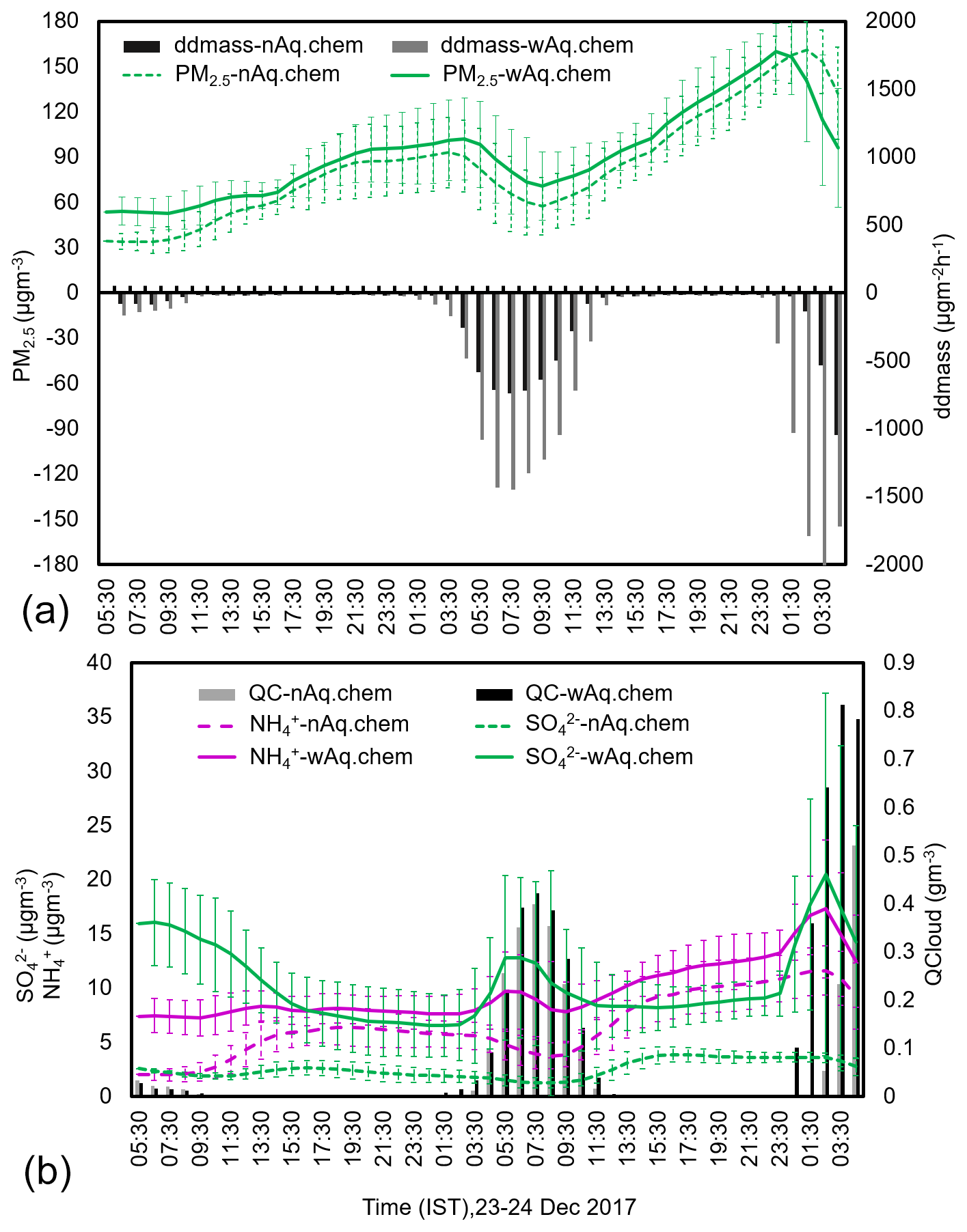
Figure 13Time series of PM2.5 and its dry deposition (ddmass) flux change (a). SO, NH, and LWC (QCloud) with and without aqueous-phase chemistry included in the model (b), averaged over the region bounded by a black rectangle in Fig. 12, for 23 and 24 December 2017.
The composition distribution of PM2.5 (Fig. 12b) has a similar distribution for the simulations with and without aqueous-phase chemistry over the NWIGP where fog did not occur. The primary aerosols (BC > 9 %, OC ∼ 16 %–30 %, and OIN > 50 %) are higher than the secondary aerosols (< 5 %). While the model requires fog for the accelerated formation of secondary inorganic aerosols, experimental data (Fig. 7) support significant formation of secondary inorganic aerosols at elevated RH levels even in haze aerosols (Acharja et al., 2022). On the other hand, the central and east IGP stations are fog-covered, and, therefore, there is an increase in secondary aerosols, especially SO and NH, when aqueous-phase chemistry is included in the simulation. SO is chemically produced via aqueous-phase chemistry in cloud water, hence the abrupt increase, whereas NH maintains a gas–aerosol and gas–cloud equilibrium with NH3 and SO via neutralizing the drop or aerosol. NO is high in the model compared to SO and NH, and it decreases by ∼ 1 %–2 % with aqueous-phase chemistry. We observe a small increase in NO during fog; however, it drops as fog intensifies, more rapidly than without aqueous-phase chemistry, likely due to an increase in dry deposition. This results in a lower average NO-to-PM2.5 ratio with aqueous-phase chemistry. Moreover, NO is high over the fog covering the CIGP and EIGP compared to the NWIGP, suggesting that transport and chemistry of NOx in the CIGP and EIGP produce more HNO3. Aerosol NO is also in equilibrium with HNO3, and it is formed only if excess NH3 is available beyond the sulfate neutralization. Thus, NH and NO changes are likely due to the change in partitioning between gas and liquid based on the production of sulfate.
PM2.5 is mostly composed of organic aerosols (OAs) over the CIGP and EIGP (Lalchandani et al., 2021; Srinivas and Sarin, 2014), whereas it is composed of OIN (dust) and OAs over the NWIGP (Ram et al., 2012a; Sharma and Mandal, 2023). Although observational studies report Cl− as one of the largest contributors (12 %–17 %) to PM2.5 after the organics (Lalchandani et al., 2021; Pant et al., 2015) during winter, Cl− is largely underestimated by the model as discussed in Sect. 4 and contributes only ∼ 3 %. A small increase (2 %–4 %) in secondary organic aerosols (SOAs) from glyoxal production in aerosols occurs for the simulation with aqueous-phase chemistry included during intense fog, suggesting there are feedbacks between cloud chemistry (without glyoxal aqueous chemistry) and aerosol chemistry. However, similarly to NO, average SOAs (ASOA (anthropogenic) + BSOA (biogenic) + GlySOA) show a decrease when aqueous-phase chemistry is included. SOA contributes significantly to organic aerosol loading over the IGP (Kaul et al., 2011; Mandariya et al., 2019).
The WRF-Chem results on aerosol composition during fog behave similarly to those of previous observational studies. For example, Ram et al. (2012a) reported an increase in EC, OC, and WSOC concentrations by ∼ 30 % during fog and haze events at Allahabad, a location in the central IGP, and a marginal increase in these constituents at Hisar (NWIGP). Several studies report an increase in inorganic ions (NH, NO, and SO) during fog over the IGP and elsewhere (Gundel et al., 1994; Ram et al., 2012a). Recent studies suggest that a significant fraction of atmospheric particulate matter in the IGP is composed of carbonaceous aerosol (∼ 30 %–35 % of the PM) and water-soluble inorganic species (∼ 10 %–20 % of the PM) during October–January when emissions from biomass burning (including residential heating) are dominant over the IGP (Ram et al., 2012b; Rengarajan et al., 2007; Tare et al., 2006).
Both the simulations with and without aqueous-phase chemistry include the AR feedback. The aqueous chemistry increases the mass of PM2.5 and the size of the aerosols, both of which contribute to AR feedback, thus increasing RH and PBL stability. The increase in RH also saturates the air, promotes aerosol growth by water uptake, and thus favors fog formation. Since the secondary inorganic aerosols are scattering aerosols, the increased scattering of radiation further reduces the solar radiation reaching the surface (Fig. 14a). Over the CIGP the presence of higher aerosol loading reduces the T2 m during the daytime, particularly on 24 December, which then reduces the PBL height and increases RH near the surface (Fig. 14b). These conditions favor fog formation over the CIGP. Furthermore, the fog water content with aqueous-phase chemistry is higher than that without aqueous-phase chemistry on 24 December post-midnight (Fig. 13b). This is likely due to the saturation of air due to an increase in RH and lower T2 m, induced by the AR feedback caused by the increase in PM2.5. Although the difference in T2 m is small (< 0.4), favorable conditions mentioned above are conducive to fog formation. Because aqueous chemistry increases sulfate concentrations, the size of the aerosols also increases. The increased aerosol size, which can grow further by water uptake, also impacts the solar radiation reaching the surface, affecting fog formation and dissipation.
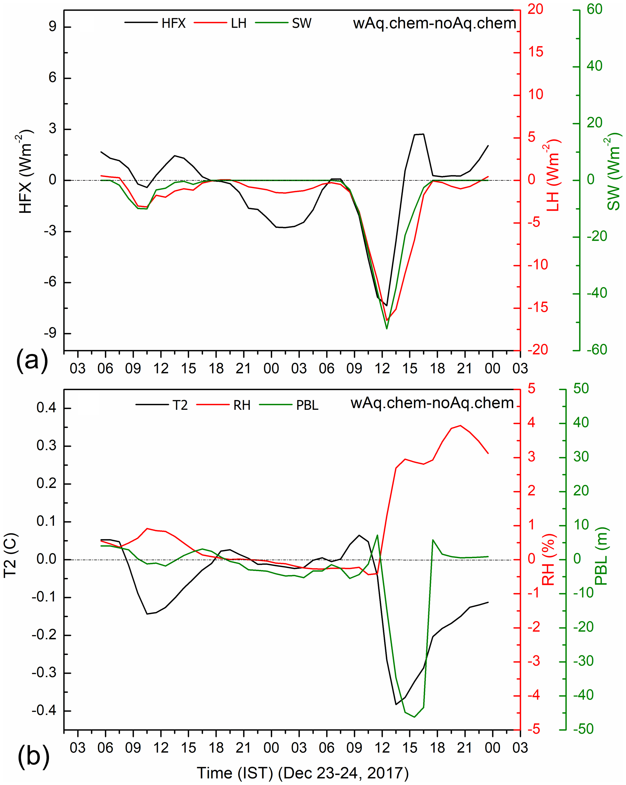
Figure 14Time series of (a) ΔHFX (sensible heat flux), ΔLH (latent heat flux), and ΔSWF (downward shortwave flux). (b) ΔT2, ΔRH, and ΔPBL over the CIGP (26–28° N, 79–83° E), for 23 and 24 December 2017. Δ denotes the difference between simulations with and without aqueous-phase chemistry.
Aerosols and their radiative effects impact fog characteristics, including the fog liquid water content (LWC), the fog lifetime over a region, and hence its spatial and temporal distribution. Variations in fog LWC in WRF-Chem contrast the fog in the CIGP and EIGP (Fig. 15) and among the three experiments (with aqueous chemistry plus AR feedback, with aqueous chemistry without AR feedback, and without aqueous chemistry but with AR feedback). WRF-Chem does not simulate fog over the NWIGP in the model for the study period. In Fig. 15, only foggy grid points are considered for the first fog event on 23–24 December. The LWC is 5 %–15 % higher with AR feedback than without AR feedback and without aqueous-phase chemistry for both the CIGP and EIGP. The interquartile range is larger for the simulation with and without AR feedback than without aqueous-phase chemistry in the CIGP, showing large variability in the LWC. On the other hand, in the EIGP the variability in LWC is greater in the simulation with AR feedback compared to the other two experiments.
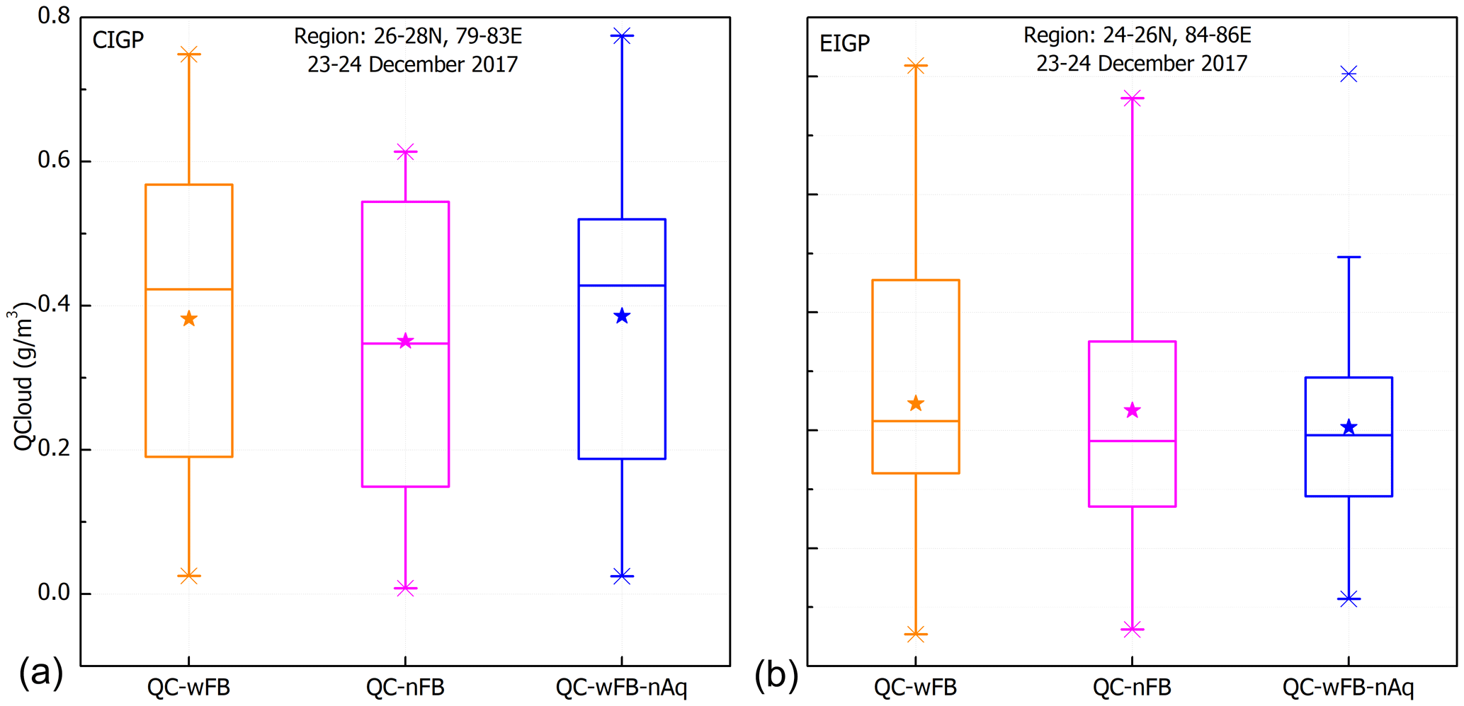
Figure 15Averages (stars), medians (horizontal lines), quartiles (boxes), maxima, and minima for LWC (QCloud) averaged over the CIGP (a) and the EIGP (b) for the fog event on 23–24 December 2017. Gold is for the simulation with AR feedback and aqueous chemistry, magenta is for the simulation with no AR feedback but includes aqueous chemistry, and blue is for the simulation with AR feedback but no aqueous chemistry. WRF-Chem does not produce fog in the NWIGP during the study period.
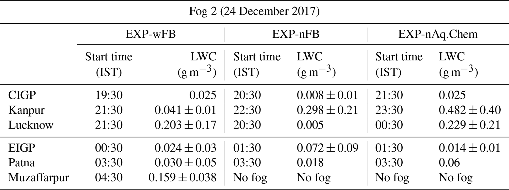
The formation and dissipation times of the two fog events for the three experiments are listed in Tables 2 and 3 for the CIGP and EIGP. The 23–24 December fog starts forming 2 h earlier, and the 24–25 December fog forms 1 h earlier, in both the CIGP and EIGP with AR feedback than without AR feedback. In the simulation without aqueous-phase chemistry, fog formation is delayed by 1–2 h compared to the simulation with aqueous chemistry plus AR feedback in the CIGP. In the EIGP the 23–24 December fog forms at the same time with AR feedback and without aqueous-phase chemistry, while the 24–25 December fog is delayed by 1 h without aqueous-phase chemistry. Fog dissipation usually occurs after sunrise when the shortwave radiative warming at the surface warms the air, which results in PBL mixing. In addition, absorbing aerosols like BC affect fog dissipation by increasing the radiative heating in and above the fog. We find an increase in BC and shortwave heating in the PBL with AR feedback (Figs. 10, 11) and warming over the CIGP with AR feedback. Fog intensity starts to decrease after 01:00 UTC (06:30 IST); however, in our study, we find that the fog dissipates completely in the afternoon (∼ 10:00 UTC or 15:30 IST) for both the simulations with AR feedback and no aqueous chemistry and 1 h later without AR feedback in the CIGP. Fog dissipation is delayed in the EIGP with AR feedback compared to without AR feedback and without aqueous-phase chemistry. In both regions, fog lifetime increases with AR feedback. Not all stations, however, show the same pattern. For example, the 23–24 December fog in Lucknow forms and dissipates at the same time for simulations with AR feedback and without aqueous-phase chemistry, and the 24–25 December fog forms later with AR feedback than without AR feedback. Patna shows no difference in the 24–25 December fog formation in all three experiments. To gain better insights into the fog timing, we recommend that simulations at higher spatial and temporal resolutions be performed to better represent the fog dynamics at point locations. Furthermore, there are other important factors to consider, e.g., improved emissions, better simulations of aerosol chemical composition, and evaluation of aerosol deposition.
Table 2Table showing the start and end time of fog 1 on 23–24 December 2017 with LWC for the sensitivity experiments, with AR feedback, no AR feedback, and no aqueous-phase chemistry.
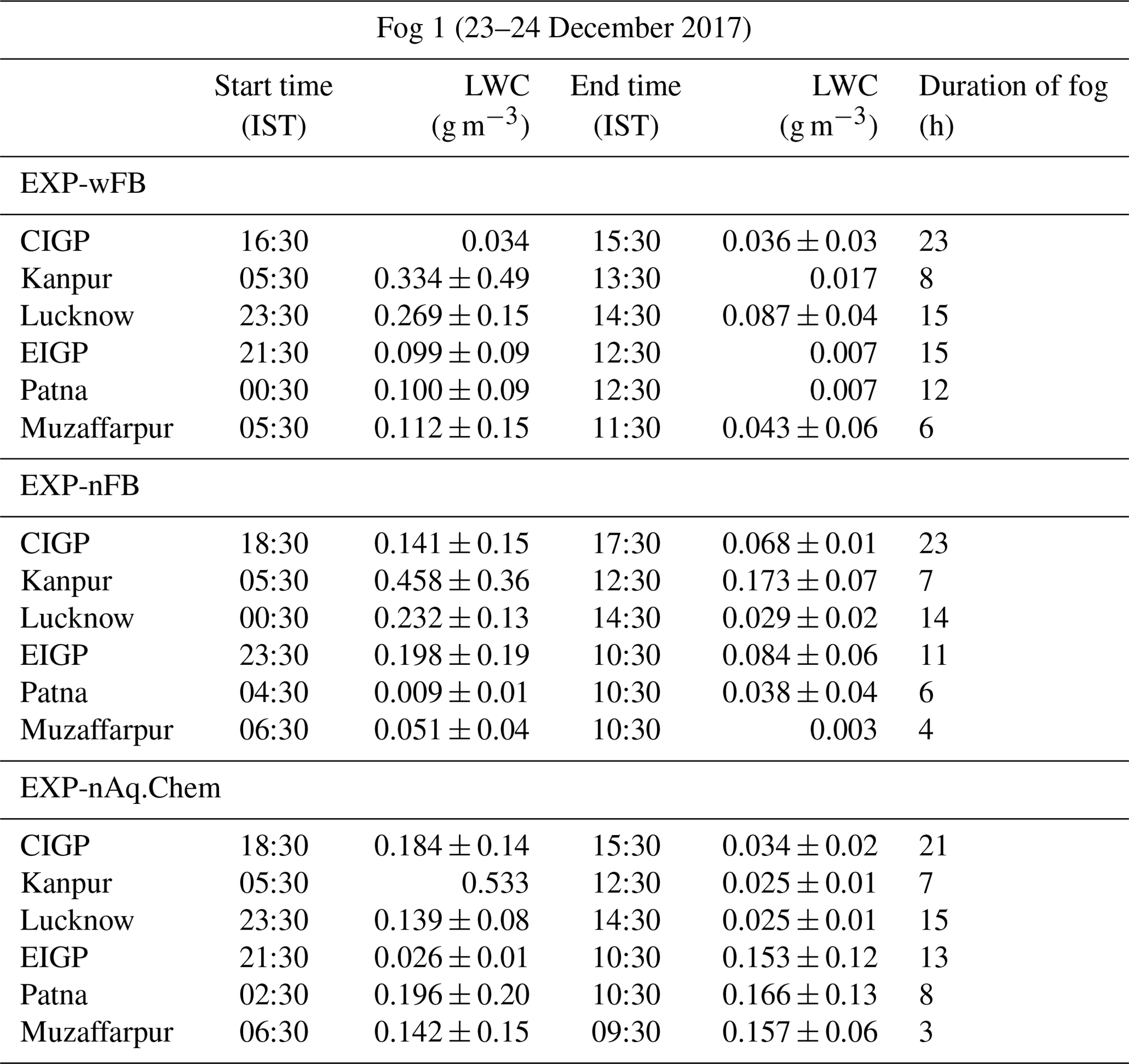
Table 3Table showing the start time of fog 2 on 24 December 2017 with LWC for the sensitivity experiments, with AR feedback, no AR feedback, and no aqueous-phase chemistry. Fog 2 end time could not be noted as the simulation ended on 25 December 2017, 00:00 UT (05:30 IST), before fog 2 dissipated.
The AR feedback and aqueous-phase chemistry have the potential to impact aerosol–fog interactions. We can learn about the effect of the aerosol–radiation interactions on CCN concentrations because the WRF-Chem model calculates the CCN concentrations at different supersaturations as a diagnostic output. We compare CCN at 0.02 % supersaturations, a value typical of fog, among the three experiments. For the 23–24 December fog in the CIGP, hourly CCN concentrations are ∼ 10 % higher for the simulations with AR feedback with or without aqueous chemistry than with no AR feedback (Fig. S8) during the first 8 h of the fog event (16:00–24:00 IST, 23 December). Surprisingly, the simulation with no aqueous chemistry has higher CCN concentrations than the simulation with aqueous chemistry, as more CCN are expected with aqueous chemistry, because aqueous chemistry adds sulfate to the aerosol mass, increasing the mass of PM2.5. Increased PM2.5 further contributes to AR feedback, increasing RH, which favors the growth of the aerosol size, categorizing more aerosols as CCN. However, the dry deposition flux (ddmass) also increases in dense fog, which causes rapid loss in CCN and activated aerosols during fog events with the AR feedback (Fig. S7) and more so without aqueous-phase chemistry. Shao et al. (2023) examined aerosol–fog interactions for two consecutive fog events by comparing WRF-Chem results with current emission strengths to those with low emission strengths. They show that the first fog event promotes formation of the second fog event, leading to wider fog distribution and longer fog lifetime favored by multiple feedbacks, including AR feedback, i.e., low temperature, high humidity, and high stability, similar to our study. While Shao et al. (2023) observe a delay in dissipation of the first fog event and early formation of the second fog event, we find an early dissipation and early formation of fog with AR feedback as discussed earlier in this section. In summary, aqueous-phase chemistry together with AR feedback promotes early formation of fog, while AR feedback alone promotes early dissipation of fog and plays a critical role in the formation and evolution of the fog over the IGP.
The effects of aerosol–radiation (AR) feedback and aqueous chemistry in air quality and fog have been assessed over the IGP. We carried out three experiments using WRF-Chem, testing different combinations of PBL schemes and meteorology initial and boundary conditions. The best representation of surface meteorology for the IGP region for the case study (20–24 December 2017) used ERA-Interim reanalysis to drive the meteorology and the ACM2 PBL scheme with soil moisture nudging to ERA-Interim. With this meteorology configuration for WRF-Chem, evaluation of aerosol concentrations with measurements and the impact of aerosols on atmospheric processes during fog were examined. Furthermore, we included trash-burning emissions to represent anthropogenic chloride aerosols in our configuration. Incorporation of trash-burning emissions did improve the model simulations of PM2.5 and better captured the day-to-day variability in PM2.5 in the IGP, yet it underestimated its magnitude compared to CPCB observations. Moreover, secondary aerosols, particularly chloride aerosols, are underestimated in the model. This underestimation is likely caused by a low bias in the residential burning emission inventory and a failure of the emission inventory to properly represent residential-sector emissions from the use of trash as cheap heating fuel. AOD regional distribution is predicted well by the model for most of the IGP. However, AOD is underestimated over the NWIGP likely due to an underestimation of fugitive emissions during wintertime cold spells.
The AR interactions showed a significant impact on meteorology and air quality over the IGP. A WRF-Chem simulation with AR interactions resulted in a lower PBL height by ∼ 50–270 m compared to a simulation without AR interactions, leading to the accumulation of aerosols and moisture near the surface. Reduced surface shortwave radiation flux and the surface-sensible and latent heat fluxes due to aerosol radiative effect suppressed the turbulence, resulting in a stable PBL. The shallow PBL further increased surface PM2.5 (> 8 µg m−3) and RH (2 %–8 %) over the IGP, and this positive feedback mechanism promoted thickening of fog over the IGP. However, an increase in absorbing aerosols in the PBL gave negative feedback, increasing the shortwave heating and temperature particularly over the CIGP. Fog forms when air is saturated, which occurs when the surface temperature is reduced or the moisture content increases, causing saturation of air. This study suggests that an increase in RH saturated the air and that the increase in aerosols favored fog formation as depicted by the thickening of fog intensity. Aqueous-phase chemistry, on the other hand, contributed significantly to secondary aerosols in the fog, especially sulfate aerosols, indicating substantial formation of secondary aerosols in the cloud. The underpredicted secondary aerosols over the NWIGP where no fog occurred imply underestimation of the formation of aerosols through gas and aerosol chemistry in the model. This underestimation could also be linked to an underestimation of pH in the default MOSAIC scheme (Ruan et al., 2022) which slows the secondary aerosol formation, an underestimation of the aqueous sulfur oxidation in haze aerosol at > 80 % RH before the onset of fog (Acharja et al., 2022), or missing multiphase oxidation processes (Wang et al., 2022). Nevertheless, we find that the model successfully simulates the same changes in the inorganic composition during fog in the IGP as those reported by observational studies referred to earlier in Sect. 6. We also observed that AR feedback with aqueous chemistry initiated the fog formation 1–2 h earlier than the initiation time in the simulation without AR feedback and without aqueous-phase chemistry, whereas AR feedback alone led to early dissipation of fog. In addition, fog acted as an important sink of aerosols in a polluted environment with increased dry deposition with cloud water. Thus, AR feedback and aqueous chemistry play a significant role in modulating the distribution and concentration of aerosols and evolution of fog in the PBL. Aerosol–cloud interactions were not investigated in this study due to the limitation of the ACM2 PBL scheme in providing necessary information with other modules in WRF. Previous studies of aerosol–fog interactions have found that ACI also promotes early onset of fog formation and increases fog duration (Maalick et al., 2016; Yan et al., 2021). While these previous studies were applied to midlatitude fog events, it is likely that ACI also plays a dominant role in the IGP fogs, suggesting that future studies are needed to fully understand aerosol effects on IGP fog events.
The large emission of aerosols and trace gases in the IGP makes the atmospheric dynamics and chemistry complex, suggesting the need for more studies using both models and ground-based measurements to better understand the processes. While all aerosol types interact with solar radiation and reduce the surface-reaching flux, the presence of absorbing aerosols in the boundary layer and its vertical distribution play an important role in modulating the meteorology over the IGP. It is therefore crucial to improve the simulation of absorbing aerosols, e.g., BC, in the vertical and at the surface to increase the accuracy in predicting the formation and dissipation of fog in this region. Emissions from burning for residential heating are an important source of aerosols in the IGP during the post-monsoon season and winter, and the inclusion of these sources in the emission inventory would improve the prediction of wintertime aerosols. For example, the underestimation of chloride aerosols in the model indicates unaccounted emission sources over the IGP and the need for more work on better quantifying trash-burning emissions, which may not only improve particulate chloride in the model but also improve simulations of other aerosol chemical components through aerosol thermodynamics. Additionally, more detailed modeling studies are required to understand the missing chemical processes, if any, in the model leading to biases in sulfate, nitrate, and ammonium partitioning between gas and aerosol phases. We find that the change in PBL height with AR feedback is sensitive to changes in LH, signifying the role of soil moisture in PBL dynamics. Several studies have reported cooling over the IGP due to an increase in irrigation (Kumar et al., 2017; Mishra et al., 2020). Further investigations into the role of irrigation in the increasing fog events over the NWIGP would help in better understanding the formation and persistence of fog over this region. It can be concluded that fog forecasting is a complex process due to the multiple factors involved, and this work suggests that AR feedback is important in fog forecasting, while aqueous-phase chemistry plays an important role in defining the composition of aerosols over the IGP.
All model simulations are archived in the NCAR campaign storage (/glade/campaign/acom/acom-weather/chandrakala) and can be accessed by contacting the corresponding author. WiFEX data can be made available by contacting Sachin D. Ghude (sachinghude@tropmet.res.in). Trash-burning emissions data are available on Mendeley Data (https://doi.org/10.17632/t2tn4t9473.1; Sinha et al., 2021). MODIS AOD retrievals can be downloaded from https://doi.org/10.5067/MODIS/MOD04_L2.061 (Levy et al., 2015a) and https://doi.org/10.5067/MODIS/MYD04_L2.061 (Levy et al., 2015b). Meteorology and aerosol data from the Central Pollution Control Board (CPCB, 2014) are available at https://airquality.cpcb.gov.in/ccr/#/caaqm-dashboard-all/caaqm-landing.
The supplement related to this article is available online at: https://doi.org/10.5194/acp-24-6635-2024-supplement.
CB: conceptualization, formal Analysis, and writing. MB: conceptualization, supervision, writing (review and editing), funding acquisition. RK: conceptualization, supervision, writing (review and editing). SDG: provision of ground-based observation data and writing (review and editing). VS and BS: provision of trash-burning emissions data and writing (review and editing).
The contact author has declared that none of the authors has any competing interests.
Publisher's note: Copernicus Publications remains neutral with regard to jurisdictional claims made in the text, published maps, institutional affiliations, or any other geographical representation in this paper. While Copernicus Publications makes every effort to include appropriate place names, the final responsibility lies with the authors.
Chandrakala Bharali is grateful to the Fulbright–Kalam Climate Fellowship program and to the Women Scientist program under Department of Science and Technology, Government of India. The NSF National Center for Atmospheric Research (NCAR) is sponsored by the U.S. National Science Foundation. The authors acknowledge the use of MODIS data from NASA's Land, Atmosphere Near-real-time Capability for EOS (LANCE) system (https://earthdata.nasa.gov/lance, last access: 21 February 2023), part of NASA's Earth Observing System Data and Information System (EOSDIS). We also acknowledge the Meteorological and Oceanographic Satellite Data Archival Centre (MOSDAC, https://www.mosdac.gov.in/, last access: 23 December 2021), Space Applications Centre, Indian Space Research Organisation, and the Government of India for INSAT-3D fog data and the Central Pollution Board of India (CPCB, https://app.cpcbccr.com/ccr/#/login, last access: 27 March 2024) for meteorology data. We would like to acknowledge the high-performance computing support from Cheyenne (https://doi.org/10.5065/D6RX99HX) provided by NCAR's Computational and Information Systems Laboratory (2019). We thank Duseong Jo, Behrooz Roozitalab, and the two anonymous reviewers for their constructive comments on the paper.
This research has been supported by the Fulbright–Kalam Climate Fellowship program under USIEF (United States–India Educational Foundation), the Women Scientist (WOS-A) program, Department of Science and Technology (DST), Government of India, and the U.S. National Science Foundation (cooperative agreement no. 1852977).
This paper was edited by Hailong Wang and reviewed by two anonymous referees.
Abdul-Razzak, H. and Ghan, S. J.: A parameterization of aerosol activation 3. Sectional representation, J. Geophys. Res.-Atmos., 107, AAC 1-1–AAC 1-6, https://doi.org/10.1029/2001JD000483, 2002.
Acharja, P., Ali, K., Ghude, S. D., Sinha, V., Sinha, B., Kulkarni, R., Gultepe, I., and Rajeevan, M. N.: Enhanced secondary aerosol formation driven by excess ammonia during fog episodes in Delhi, India, Chemosphere, 289, 133155, https://doi.org/10.1016/j.chemosphere.2021.133155, 2022.
Anu Rani Sharma, Shailesh Kumar Kharol, Badarinath, K. V. S., and Darshan Singh: Impact of agriculture crop residue burning on atmospheric aerosol loading – a study over Punjab State, India, Ann. Geophys., 28, 367–379, https://doi.org/10.5194/angeo-28-367-2010, 2010.
Arun, S. H., Sharma, S. K., Chaurasia, S., Vaishnav, R., and Kumar, R.: Fog/low clouds detection over the delhi earth station using the ceilometer and the insat-3d/3dr satellite data, Int. J. Remote Sens., 39, 4130–4144, https://doi.org/10.1080/01431161.2018.1454624, 2018.
Badarinath, K. V. S., Kumar Kharol, S., and Rani Sharma, A.: Long-range transport of aerosols from agriculture crop residue burning in Indo-Gangetic Plains—A study using LIDAR, ground measurements and satellite data, J. Atmos. Sol.-Terr. Phy., 71, 112–120, https://doi.org/10.1016/j.jastp.2008.09.035, 2009.
Banerjee, S. and Padmakumari, B.: Spatiotemporal variability and evolution of day and night winter fog over the Indo Gangetic Basin using INSAT-3D and comparison with surface visibility and aerosol optical depth, Sci. Total Environ., 745, 140962, https://doi.org/10.1016/j.scitotenv.2020.140962, 2020.
Behera, S. N. and Sharma, M.: Reconstructing primary and secondary components of PM2.5 composition for an Urban Atmosphere, Aerosol Sci. Tech., 44, 983–992, https://doi.org/10.1080/02786826.2010.504245, 2010.
Bergot, T. and Guedalia, D.: Numerical Forecasting of Radiation Fog. Part I: Numerical Model and Sensitivity Tests, Mon. Weather Rev., 122, 1218–1230, https://doi.org/10.1175/1520-0493(1994)122<1218:NFORFP>2.0.CO;2, 1994.
Bharali, C., Nair, V. S., Chutia, L., and Babu, S. S.: Modeling of the Effects of Wintertime Aerosols on Boundary Layer Properties Over the Indo Gangetic Plain, J. Geophys. Res.-Atmos., 124, 4141–4157, https://doi.org/10.1029/2018JD029758, 2019.
Bodaballa, J. K., Geresdi, I., Ghude, S. D., and Salma, I.: Numerical simulation of the microphysics and liquid chemical processes occur in fog using size resolving bin scheme, Atmos. Res., 266, 105972, https://doi.org/10.1016/j.atmosres.2021.105972, 2022.
Boutle, I., Price, J., Kudzotsa, I., Kokkola, H., and Romakkaniemi, S.: Aerosol–fog interaction and the transition to well-mixed radiation fog, Atmos. Chem. Phys., 18, 7827–7840, https://doi.org/10.5194/acp-18-7827-2018, 2018.
Bran, S. H. and Srivastava, R.: Investigation of PM2.5 mass concentration over India using a regional climate model, Environ. Pollut., 224, 484–493, https://doi.org/10.1016/j.envpol.2017.02.030, 2017.
Central Pollution Control Board (CPCB): https://airquality.cpcb.gov.in/ccr/#/caaqm-dashboard-all/caaqm-landing, last access: 27 March 2014.
Chapman, E. G., Gustafson Jr., W. I., Easter, R. C., Barnard, J. C., Ghan, S. J., Pekour, M. S., and Fast, J. D.: Coupling aerosol-cloud-radiative processes in the WRF-Chem model: Investigating the radiative impact of elevated point sources, Atmos. Chem. Phys., 9, 945–964, https://doi.org/10.5194/acp-9-945-2009, 2009.
Chaudhary, P., Garg, S., George, T., Shabin, M., Saha, S., Subodh, S., and Sinha, B.: Underreporting and open burning – the two largest challenges for sustainable waste management in India, Resour. Conserv. Recy., 175, 105865, https://doi.org/10.1016/j.resconrec.2021.105865, 2021.
Chaurasia, S. and Gohil, B. S.: Detection of Day Time Fog over India Using INSAT-3D Data, IEEE J. Sel. Top. Appl., 8, 4524–4530, https://doi.org/10.1109/JSTARS.2015.2493000, 2015.
Chaurasia, S. and Jenamani, R. K.: Detection of Fog Using Temporally Consistent, IEEE J. Sel. Top. Appl., 10, 5307–5313, https://doi.org/10.1109/JSTARS.2017.2759197, 2017.
Chen, C., Zhang, M., Perrie, W., Chang, R., Chen, X., Duplessis, P., and Wheeler, M.: Boundary Layer Parameterizations to Simulate Fog Over Atlantic Canada Waters, Earth and Space Science, 7, e2019EA000703, https://doi.org/10.1029/2019EA000703, 2020.
Chen, F. and Dudhia, J.: Coupling and advanced land surface-hydrology model with the Penn State-NCAR MM5 modeling system. Part I: Model implementation and sensitivity, Mon. Weather Rev., 129, 569–585, https://doi.org/10.1175/1520-0493(2001)129<0569:CAALSH>2.0.CO;2, 2001.
Computational and Information Systems Laboratory: Cheyenne: HPE/SGI ICE XA System (NCAR Community Computing), National Center for Atmospheric Research, Boulder, CO, https://doi.org/10.5065/D6RX99HX, 2019.
David, L. M., Ravishankara, A. R., Kodros, J. K., Venkataraman, C., Sadavarte, P., Pierce, J. R., Chaliyakunnel, S., and Millet, D. B.: Aerosol Optical Depth Over India, J. Geophys. Res.-Atmos., 123, 3688–3703, https://doi.org/10.1002/2017JD027719, 2018.
Debnath, S., Karumuri, R. K., Govardhan, G., Jat, R., Saini, H., Vispute, A., Kulkarni, S. H., Jena, C., Kumar, R., Chate, D. M., and Ghude, S. D.: Implications of Implementing Promulgated and Prospective Emission Regulations on Air Quality and Health in India during 2030, Aerosol Air Qual. Res., 22, 220112, https://doi.org/10.4209/aaqr.220112, 2022.
Deshpande, P., Meena, D., Tripathi, S., Bhattacharya, A., and Verma, M. K.: Event-based fog climatology and typology for cities in Indo-Gangetic plains, Urban Climate, 51, 101642, https://doi.org/10.1016/j.uclim.2023.101642, 2023.
Dey, S. and Di Girolamo, L.: A decade of change in aerosol properties over the Indian subcontinent, Geophys. Res. Lett., 38, L14811, https://doi.org/10.1029/2011GL048153, 2011.
Dey, S. and Tripathi, S. N.: Estimation of aerosol optical properties and radiative effects in the Ganga basin, northern India, during the wintertime, J. Geophys. Res.-Atmos., 112, D03203, https://doi.org/10.1029/2006JD007267, 2007.
Dhangar, N. G., Lal, D. M., Ghude, S. D., Kulkarni, R., Parde, A. N., Pithani, P., Niranjan, K., Prasad, D. S. V. V. D., Jena, C., Sajjan, V. S., Prabhakaran, T., Karipot, A. K., Jenamani, R. K., Singh, S., and Rajeevan, M.: On the Conditions for Onset and Development of Fog Over New Delhi: An Observational Study from the WiFEX, Pure Appl. Geophys., 178, 3727–3746, https://doi.org/10.1007/s00024-021-02800-4, 2021.
Ding, A. J., Huang, X., Nie, W., Sun, J. N., Kerminen, V. M., Petäjä, T., Su, H., Cheng, Y. F., Yang, X. Q., Wang, M. H., Chi, X. G., Wang, J. P., Virkkula, A., Guo, W. D., Yuan, J., Wang, S. Y., Zhang, R. J., Wu, Y. F., Song, Y., Zhu, T., Zilitinkevich, S., Kulmala, M., and Fu, C. B.: Enhanced haze pollution by black carbon in megacities in China, Geophys. Res. Lett., 43, 2873–2879, https://doi.org/10.1002/2016GL067745, 2016.
Easter, R. C., Ghan, S. J., Zhang, Y., Saylor, R. D., Chapman, E. G., Laulainen, N. S., Abdul-Razzak, H., Leung, L. R., Bian, X., and Zaveri, R. A.: MIRAGE: Model description and evaluation of aerosols and trace gases, J. Geophys. Res.-Atmos., 109, D20210, https://doi.org/10.1029/2004JD004571, 2004.
Emmons, L. K., Walters, S., Hess, P. G., Lamarque, J.-F., Pfister, G. G., Fillmore, D., Granier, C., Guenther, A., Kinnison, D., Laepple, T., Orlando, J., Tie, X., Tyndall, G., Wiedinmyer, C., Baughcum, S. L., and Kloster, S.: Description and evaluation of the Model for Ozone and Related chemical Tracers, version 4 (MOZART-4), Geosci. Model Dev., 3, 43–67, https://doi.org/10.5194/gmd-3-43-2010, 2010.
Emmons, L. K., Schwantes, R. H., Orlando, J. J., Tyndall, G., Kinnison, D., Lamarque, J. F., Marsh, D., Mills, M. J., Tilmes, S., Bardeen, C., Buchholz, R. R., Conley, A., Gettelman, A., Garcia, R., Simpson, I., Blake, D. R., Meinardi, S., and Pétron, G.: The Chemistry Mechanism in the Community Earth System Model Version 2 (CESM2), J. Adv. Model. Earth Sy., 12, e2019MS001882, https://doi.org/10.1029/2019MS001882, 2020.
Fahey, K. M. and Pandis, S. N.: Optimizing model performance: variable size resolution in cloud chemistry modeling, Atmos. Environ., 35, 4471–4478, https://doi.org/10.1016/S1352-2310(01)00224-2, 2001.
Fast, J. D., Gustafson Jr, W. I., Easter, R. C., Zaveri, R. A., Barnard, J. C., Chapman, E. G., Grell, G. A., and Peckham, S. E.: Evolution of ozone, particulates, and aerosol direct forcing in an urban area using a new fully-coupled meteorology, chemistry, and aerosol model, J. Geophys. Res, 111, D21305, https://doi.org/10.1029/2005JD006721, 2006.
Gautam, R., Hsu, N. C., Kafatos, M., and Tsay, S.: Influences of winter haze on fog/low cloud over the Indo-Gangetic plains, J. Geophys. Res., 112, D05207, https://doi.org/10.1029/2005JD007036, 2007.
Ghude, S. D., Kulkarni, S. H., Jena, C., Pfister, G. G., Beig, G., Fadnavis, S., and Van Der, R. J.: Application of satellite observations for identifying regions of dominant sources of nitrogen oxides over the indian subcontinent, J. Geophys. Res.-Atmos., 118, 1075–1089, https://doi.org/10.1029/2012JD017811, 2013.
Ghude, S. D., Chate, D. M., Jena, C., Beig, G., Kumar, R., Barth, M. C., Pfister, G. G., Fadnavis, S., and Pithani, P.: Premature mortality in India due to PM2.5 and ozone exposure, Geophys. Res. Lett., 43, 4650–4658, https://doi.org/10.1002/2016GL068949, 2016.
Ghude, S. D., Bhat, G. S., Prabhakaran, T., Jenamani, R. K., Chate, D. M., Safai, P. D., Karipot, A. K., Konwar, M., Pithani, P., Sinha, V., Rao, P. S. P., Dixit, S. A., Tiwari, S., Todekar, K., Varpe, S., Srivastava, A. K., Bisht, D. S., Murugavel, P., Ali, K., Mina, U., Dharua, M., Jaya Rao, Y., Padmakumari, B., Hazra, A., Nigam, N., Shende, U., Lal, D. M., Chandra, B. P., Mishra, A. K., Kumar, A., Hakkim, H., Pawar, H., Acharja, P., Kulkarni, R., Subharthi, C., Balaji, B., Varghese, M., Bera, S., and Rajeevan, M.: Winter fog experiment over the Indo-Gangetic plains of India, Curr. Sci., 112, 767–784, https://api.semanticscholar.org/CorpusID:99884123 (last access: 3 June 2024), 2017.
Ghude, S. D., Kumar, R., Jena, C., Debnath, S., Kulkarni, R. G., Alessandrini, S., Biswas, M., Kulkrani, S., Pithani, P., Kelkar, S., Sajjan, V., Chate, D. M., Soni, V. K., Singh, S., Nanjundiah, R. S., and Rajeevan, M.: Evaluation of PM2.5 forecast using chemical data assimilation in the WRF-Chem model: A novel initiative under the Ministry of Earth Sciences Air Quality Early Warning System for Delhi, India, Curr. Sci., 118, 1803–1815, https://api.semanticscholar.org/CorpusID:221212334 (last access: 3 June 2024), 2020.
Ghude, S. D., Jenamani, R. K., Kulkarni, R., Wagh, S., Dhangar, N. G., Parde, A. N., Acharja, P., Lonkar, P., Govardhan, G., Yadav, P., Vispute, A., Debnath, S., Lal, D. M., Bisht, D. S., Jena, C., Pawar, P. V., Dhankhar, S. S., Sinha, V., Chate, D. M., Safai, P. D., Nigam, N., Konwar, M., Hazra, A., Dharmaraj, T., Gopalkrishnan, V., Padmakumari, B., Gultepe, I., Biswas, M., Karipot, A. K., Prabhakaran, T., Nanjundiah, R. S., and Rajeevan, M.: WiFEX Walk into the Warm Fog over Indo-Gangetic Plain Region, B. Am. Meteorol. Soc., 104, E980–E1005, https://doi.org/10.1175/BAMS-D-21-0197.1, 2023.
Govardhan, G., Nanjundiah, R. S., Satheesh, S. K., Krishnamoorthy, K., and Kotamarthi, V. R.: Performance of WRF-chem over indian region: Comparison with measurements, J. Earth Syst. Sci., 124, 875–896, https://doi.org/10.1007/s12040-015-0576-7, 2015.
Grell, G. A., Peckham, S. E., Schmitz, R., McKeen, S. A., Frost, G., Skamarock, W. C., and Eder, B.: Fully coupled “online” chemistry within the WRF model, Atmos. Environ., 39, 6957–6975, https://doi.org/10.1016/j.atmosenv.2005.04.027, 2005.
Guenther, A., Karl, T., Harley, P., Wiedinmyer, C., Palmer, P. I., and Geron, C.: Estimates of global terrestrial isoprene emissions using MEGAN (Model of Emissions of Gases and Aerosols from Nature), Atmos. Chem. Phys., 6, 3181–3210, https://doi.org/10.5194/acp-6-3181-2006, 2006.
Gundel, L. A., Benner, W. H., and Hansen, A. D. A.: Chemical composition of fog water and interstitial aerosol in Berkeley, California, Atmos. Environ., 28, 2715–2725, https://doi.org/10.1016/1352-2310(94)90443-X, 1994.
Gunwani, P. and Mohan, M.: Sensitivity of WRF model estimates to various PBL parameterizations in different climatic zones over India, Atmos. Res., 194, 43–65, https://doi.org/10.1016/j.atmosres.2017.04.026, 2017.
Gupta, T. and Mandariya, A.: Sources of submicron aerosol during fog-dominated wintertime at Kanpur, Environ. Sci. Pollut. R., 20, 5615–5629, https://doi.org/10.1007/s11356-013-1580-6, 2013.
Hakkim, H., Sinha, V., Chandra, B. P., Kumar, A., Mishra, A. K., Sinha, B., Sharma, G., Pawar, H., Sohpaul, B., Ghude, S. D., Pithani, P., Kulkarni, R., Jenamani, R. K., and Rajeevan, M.: Volatile organic compound measurements point to fog-induced biomass burning feedback to air quality in the megacity of Delhi, Sci. Total Environ., 689, 295–304, https://doi.org/10.1016/j.scitotenv.2019.06.438, 2019.
Hong, S. Y., Noh, Y., and Dudhia, J.: A new vertical diffusion package with an explicit treatment of entrainment processes, Mon. Weather Rev., 134, 2318–2341, https://doi.org/10.1175/MWR3199.1, 2006.
Jacobson, M. Z., Turco, R. P., Jensen, E. J., and Toon, O. B.: Modeling coagulation among particles of different composition and size, Atmos. Environ., 28, 1327–1338, https://doi.org/10.1016/1352-2310(94)90280-1, 1994.
Jain, S., Sharma, S. K., Vijayan, N., and Mandal, T. K.: Seasonal characteristics of aerosols (PM2.5 and PM10) and their source apportionment using PMF: A four year study over Delhi, India, Environ. Pollut., 262, 114337, https://doi.org/10.1016/j.envpol.2020.114337, 2020.
Jena, C., Ghude, S. D., Kulkarni, R., Debnath, S., Kumar, R., Soni, V. K., Acharja, P., Kulkarni, S. H., Khare, M., Kaginalkar, A. J., Chate, D. M., Ali, K., Nanjundiah, R. S., and Rajeevan, M. N.: Evaluating the sensitivity of fine particulate matter (PM2.5) simulations to chemical mechanism in Delhi, Atmos. Chem. Phys. Discuss. [preprint], https://doi.org/10.5194/acp-2020-673, 2020.
Jena, C., Ghude, S. D., Kumar, R., Debnath, S., Govardhan, G., Soni, V. K., Kulkarni, S. H., Beig, G., Nanjundiah, R. S., and Rajeevan, M.: Performance of high resolution (400 m) PM2.5 forecast over Delhi, Sci. Rep., 11, 1–9, https://doi.org/10.1038/s41598-021-83467-8, 2021.
Jenamani, R. K.: Alarming rise in fog and pollution causing a fall in maximum temperature over Delhi, Curr. Sci., 93, 314–322, 2007.
Jethva, H., Chand, D., Torres, O., Gupta, P., Lyapustin, A., and Patadia, F.: Agricultural burning and air quality over northern india: A synergistic analysis using nasa's a-train satellite data and ground measurements, Aerosol Air Qual. Res., 18, 1756–1773, https://doi.org/10.4209/aaqr.2017.12.0583, 2018.
Katata, G., Chino, M., Kobayashi, T., Terada, H., Ota, M., Nagai, H., Kajino, M., Draxler, R., Hort, M. C., Malo, A., Torii, T., and Sanada, Y.: Detailed source term estimation of the atmospheric release for the Fukushima Daiichi Nuclear Power Station accident by coupling simulations of an atmospheric dispersion model with an improved deposition scheme and oceanic dispersion model, Atmos. Chem. Phys., 15, 1029–1070, https://doi.org/10.5194/acp-15-1029-2015, 2015.
Kaul, D. S., Gupta, T., Tripathi, S. N., Tare, V., and Collett, J. L.: Secondary organic aerosol: A comparison between foggy and nonfoggy days, Environ. Sci. Technol., 45, 7307–7313, https://doi.org/10.1021/es201081d, 2011.
Kedia, S., Ramachandran, S., Holben, B. N., and Tripathi, S. N.: Quantification of aerosol type, and sources of aerosols over the Indo-Gangetic Plain, Atmos. Environ., 98, 607–619, https://doi.org/10.1016/j.atmosenv.2014.09.022, 2014.
Knote, C., Tuccella, P., Curci, G., Emmons, L., Orlando, J. J., Madronich, S., Baró, R., Jiménez-Guerrero, P., Luecken, D., Hogrefe, C., Forkel, R., Werhahn, J., Hirtl, M., Pérez, J. L., San José, R., Giordano, L., Brunner, D., Yahya, K., and Zhang, Y.: Influence of the choice of gas-phase mechanism on predictions of key gaseous pollutants during the AQMEII phase-2 intercomparison, Atmos. Environ., 115, 553–568, https://doi.org/10.1016/j.atmosenv.2014.11.066, 2014.
Krishna, R. K., Panicker, A. S., Yusuf, A. M., and Ullah, B. G.: On the contribution of particulate matter (PM2.5) to direct radiative forcing over two urban environments in India, Aerosol Air Qual. Res., 19, 399–410, https://doi.org/10.4209/aaqr.2018.04.0128, 2019.
Krishna Moorthy, K., Suresh Babu, S., Manoj, M. R., and Satheesh, S. K.: Buildup of aerosols over the Indian Region, Geophys. Res. Lett., 40, 1011–1014, https://doi.org/10.1002/grl.50165, 2013.
Kulkarni, R., Jenamani, R. K., Pithani, P., and Konwar, M.: Loss to Aviation Economy Due to Winter Fog in New Delhi during the Winter of 2011–2016, Atmosphere, 10, 198, https://doi.org/10.3390/atmos10040198, 2019.
Kulkarni, S. H., Ghude, S. D., Jena, C., Karumuri, R. K., Sinha, B., Sinha, V., Kumar, R., Soni, V. K., and Khare, M.: How Much Does Large-Scale Crop Residue Burning Affect the Air Quality in Delhi?, Environ. Sci. Technol., 54, 4790–4799, https://doi.org/10.1021/acs.est.0c00329, 2020.
Kumar, A. and Sarin, M. M.: Aerosol iron solubility in a semi-arid region: temporal trend and impact of anthropogenic sources, Tellus B, 62, 125–132, https://doi.org/10.1111/j.1600-0889.2009.00448.x, 2010.
Kumar, A., Hakkim, H., Sinha, B., and Sinha, V.: Gridded 1 km × 1 km emission inventory for paddy stubble burning emissions over north-west India constrained by measured emission factors of 77 VOCs and district-wise crop yield data, Sci. Total Environ., 789, 148064, https://doi.org/10.1016/j.scitotenv.2021.148064, 2021.
Kumar, M., Parmar, K. S., Kumar, D. B., Mhawish, A., Broday, D. M., Mall, R. K., and Banerjee, T.: Long-term aerosol climatology over Indo-Gangetic Plain: Trend, prediction and potential source fields, Atmos. Environ., 180, 37–50, https://doi.org/10.1016/j.atmosenv.2018.02.027, 2018.
Kumar, R., Barth, M. C., Pfister, G. G., Nair, V. S., Ghude, S. D., and Ojha, N.: What controls the seasonal cycle of black carbon aerosols in India?, J. Geophys. Res.-Atmos., 120, 7788–7812, https://doi.org/10.1002/2015JD023298, 2015.
Kumar, R., Ghude, S. D., Biswas, M., Jena, C., Alessandrini, S., Debnath, S., Kulkarni, S., Sperati, S., Soni, V. K., Nanjundiah, R. S., and Rajeevan, M.: Enhancing Accuracy of Air Quality and Temperature Forecasts During Paddy Crop Residue Burning Season in Delhi Via Chemical Data Assimilation, J. Geophys. Res.-Atmos., 125, e2020JD033019, https://doi.org/10.1029/2020JD033019, 2020.
Kumar, R., Mishra, V., Buzan, J., Kumar, R., Shindell, D., and Huber, M.: Dominant control of agriculture and irrigation on urban heat island in India, Sci. Rep., 7, 14054, https://doi.org/10.1038/s41598-017-14213-2, 2017.
Lalchandani, V., Kumar, V., Tobler, A., M. Thamban, N., Mishra, S., Slowik, J. G., Bhattu, D., Rai, P., Satish, R., Ganguly, D., Tiwari, S., Rastogi, N., Tiwari, S., Močnik, G., Prévôt, A. S. H., and Tripathi, S. N.: Real-time characterization and source apportionment of fine particulate matter in the Delhi megacity area during late winter, Sci. Total Environ., 770, 145324, https://doi.org/10.1016/j.scitotenv.2021.145324, 2021.
Lelieveld, J., Evans, J. S., Fnais, M., Giannadaki, D., and Pozzer, A.: The contribution of outdoor air pollution sources to premature mortality on a global scale, Nature, 525, 367–371, https://doi.org/10.1038/nature15371, 2015.
Levy, R., Hsu, C., et al.: MODIS Atmosphere L2 Aerosol Product, NASA MODIS Adaptive Processing System, Goddard Space Flight Center [data set], USA, https://doi.org/10.5067/MODIS/MOD04_L2.061, 2015a.
Levy, R., Hsu, C., et al.: MODIS Atmosphere L2 Aerosol Product, NASA MODIS Adaptive Processing System, Goddard Space Flight Center [data set], USA, https://doi.org/10.5067/MODIS/MYD04_L2.061, 2015b.
Ma, Y., Brooks, S. D., Vidaurre, G., Khalizov, A. F., Wang, L., and Zhang, R.: Rapid modification of cloud-nucleating ability of aerosols by biogenic emissions, Geophys. Res. Lett., 40, 6293–6297, https://doi.org/10.1002/2013GL057895, 2013.
Maalick, Z., Kühn, T., Korhonen, H., Kokkola, H., Laaksonen, A., and Romakkaniemi, S.: Effect of aerosol concentration and absorbing aerosol on the radiation fog life cycle, Atmos. Environ., 133, 26–33, https://doi.org/10.1016/j.atmosenv.2016.03.018, 2016.
Mandariya, A. K., Gupta, T., and Tripathi, S. N.: Effect of aqueous-phase processing on the formation and evolution of organic aerosol (OA) under different stages of fog life cycles, Atmos. Environ., 206, 60–71, https://doi.org/10.1016/j.atmosenv.2019.02.047, 2019.
Martin, L. R. and Good, T. W.: Catalyzed oxidation of sulfur dioxide in solution: The iron-manganese synergism, Atmos. Environ. A-Gen., 25, 2395–2399, https://doi.org/10.1016/0960-1686(91)90113-L, 1991.
Mishra, V., Ambika, A. K., Asoka, A., Aadhar, S., Buzan, J., Kumar, R., and Huber, M.: Moist heat stress extremes in India enhanced by irrigation, Nat. Geosci., 13, 722–728, https://doi.org/10.1038/s41561-020-00650-8, 2020.
Mohan, M. and Bhati, S.: Analysis of WRF Model Performance over Subtropical Region of Delhi, India, Adv. Meteorol., 2011, 621235, https://doi.org/10.1155/2011/621235, 2011.
Mohan, M. and Gupta, M.: Sensitivity of PBL parameterizations on PM10 and ozone simulation using chemical transport model WRF-Chem over a sub-tropical urban airshed in India, Atmos. Environ., 185, 53–63, https://doi.org/10.1016/j.atmosenv.2018.04.054, 2018.
Moore, R. H., Cerully, K., Bahreini, R., Brock, C. A., Middlebrook, A. M., and Nenes, A.: Hygroscopicity and composition of California CCN during summer 2010, J. Geophys. Res.-Atmos., 117, 1–14, https://doi.org/10.1029/2011JD017352, 2012.
Nagar, P. K., Singh, D., Sharma, M., Kumar, A., Aneja, V. P., George, M. P., Agarwal, N., and Shukla, S. P.: Characterization of PM2.5 in Delhi: role and impact of secondary aerosol, burning of biomass, and municipal solid waste and crustal matter, Environ. Sci. Pollut. R., 24, 25179–25189, https://doi.org/10.1007/s11356-017-0171-3, 2017.
Nagpure, A. S., Ramaswami, A., and Russell, A.: Characterizing the Spatial and Temporal Patterns of Open Burning of Municipal Solid Waste (MSW) in Indian Cities, Environ. Sci. Technol., 49, 12904–12912, https://doi.org/10.1021/acs.est.5b03243, 2015.
Neu, J. L. and Prather, M. J.: Toward a more physical representation of precipitation scavenging in global chemistry models: cloud overlap and ice physics and their impact on tropospheric ozone, Atmos. Chem. Phys., 12, 3289–3310, https://doi.org/10.5194/acp-12-3289-2012, 2012.
Ojha, N., Sharma, A., Kumar, M., Girach, I., Ansari, T. U., Sharma, S. K., Singh, N., Pozzer, A., and Gunthe, S. S.: On the widespread enhancement in fine particulate matter across the Indo-Gangetic Plain towards winter, Sci. Rep., 10, 1–9, https://doi.org/10.1038/s41598-020-62710-8, 2020.
Pan, X., Chin, M., Gautam, R., Bian, H., Kim, D., Colarco, P. R., Diehl, T. L., Takemura, T., Pozzoli, L., Tsigaridis, K., Bauer, S., and Bellouin, N.: A multi-model evaluation of aerosols over South Asia: common problems and possible causes, Atmos. Chem. Phys., 15, 5903–5928, https://doi.org/10.5194/acp-15-5903-2015, 2015.
Pant, P., Shukla, A., Kohl, S. D., Chow, J. C., Watson, J. G., and Harrison, R. M.: Characterization of ambient PM2.5 at a pollution hotspot in New Delhi, India and inference of sources, Atmos. Environ., 109, 178–189, https://doi.org/10.1016/j.atmosenv.2015.02.074, 2015.
Patil, R. S., Kumar, R., Menon, R., Shah, M. K., and Sethi, V.: Development of particulate matter speciation profiles for major sources in six cities in India, Atmos. Res., 132–133, 1–11, https://doi.org/10.1016/j.atmosres.2013.04.012, 2013.
Pawar, H. and Sinha, B.: Residential heating emissions (can) exceed paddy-residue burning emissions in rural northwest India, Atmos. Environ., 269, 118846, https://doi.org/10.1016/j.atmosenv.2021.118846, 2022.
Pawar, P. V., Ghude, S. D., Govardhan, G., Acharja, P., Kulkarni, R., Kumar, R., Sinha, B., Sinha, V., Jena, C., Gunwani, P., Adhya, T. K., Nemitz, E., and Sutton, M. A.: Chloride (HCl/Cl−) dominates inorganic aerosol formation from ammonia in the Indo-Gangetic Plain during winter: modeling and comparison with observations, Atmos. Chem. Phys., 23, 41–59, https://doi.org/10.5194/acp-23-41-2023, 2023.
Pithani, P., Ghude, S. D., Chennu, V. N., Kulkarni, R. G., Steeneveld, G. J., Sharma, A., Prabhakaran, T., Chate, D. M., Gultepe, I., Jenamani, R. K., and Madhavan, R.: WRF Model Prediction of a Dense Fog Event Occurred During the Winter Fog Experiment (WIFEX), Pure Appl. Geophys., 176, 1827–1846, https://doi.org/10.1007/s00024-018-2053-0, 2019.
Pithani, P., Ghude, S. D., Jenamani, R. K., Biswas, M., Naidu, C. V., Debnath, S., Kulkarni, R., Dhangar, N. G., Jena, C., Hazra, A., Phani, R., Mukhopadhyay, P., Prabhakaran, T., Nanjundiah, R. S., and Rajeevan, M.: Real-time forecast of dense fog events over Delhi: The performance of the wrf model during the wifex field campaign, Weather Forecast., 35, 739–756, https://doi.org/10.1175/WAF-D-19-0104.1, 2020.
Pleim, J. E.: A combined local and nonlocal closure model for the atmospheric boundary layer. Part I: Model description and testing, J. Appl. Meteorol. Clim., 46, 1383–1395, https://doi.org/10.1175/JAM2539.1, 2007a.
Pleim, J. E.: A combined local and nonlocal closure model for the atmospheric boundary layer. Part II: Application and evaluation in a mesoscale meteorological model, J. Appl. Meteorol. Clim., 46, 1396–1409, https://doi.org/10.1175/JAM2534.1, 2007b.
Pleim, J. E. and Chang, J. S.: A non-local closure model for vertical mixing in the convective boundary layer, Atmos. Environ. A.-Gen., 26, 965–981, https://doi.org/10.1016/0960-1686(92)90028-J, 1992.
Pleim, J. E. and Gilliam, R.: An indirect data assimilation scheme for deep soil temperature in the Pleim-Xiu land surface model, J. Appl. Meteorol. Clim., 48, 1362–1376, https://doi.org/10.1175/2009JAMC2053.1, 2009.
Pleim, J. E. and Xiu, A.: Development of a land surface model. Part II: Data assimilation, J. Appl. Meteorol., 42, 1811–1822, https://doi.org/10.1175/1520-0450(2003)042<1811:DOALSM>2.0.CO;2, 2003.
Powers, J. G., Klemp, J. B., Skamarock, W. C., Davis, C. A., Dudhia, J., Gill, D. O., Coen, J. L., Gochis, D. J., Ahmadov, R., Peckham, S. E., Grell, G. A., Michalakes, J., Trahan, S., Benjamin, S. G., Alexander, C. R., Dimego, G. J., Wang, W., Schwartz, C. S., Romine, G. S., Liu, Z., Snyder, C., Chen, F., Barlage, M. J., Yu, W., and Duda, M. G.: The weather research and forecasting model: Overview, system efforts, and future directions, B. Am. Meteorol. Soc., 98, 1717–1737, https://doi.org/10.1175/BAMS-D-15-00308.1, 2017.
Pye, H. O. T., Nenes, A., Alexander, B., Ault, A. P., Barth, M. C., Clegg, S. L., Collett Jr., J. L., Fahey, K. M., Hennigan, C. J., Herrmann, H., Kanakidou, M., Kelly, J. T., Ku, I.-T., McNeill, V. F., Riemer, N., Schaefer, T., Shi, G., Tilgner, A., Walker, J. T., Wang, T., Weber, R., Xing, J., Zaveri, R. A., and Zuend, A.: The acidity of atmospheric particles and clouds, Atmos. Chem. Phys., 20, 4809–4888, https://doi.org/10.5194/acp-20-4809-2020, 2020.
Ram, K., Sarin, M. M., Sudheer, A. K., and Rengarajan, R.: Carbonaceous and secondary inorganic aerosols during wintertime fog and haze over urban sites in the Indo-Gangetic plain, Aerosol Air Qual. Res., 12, 355–366, https://doi.org/10.4209/aaqr.2011.07.0105, 2012a.
Ram, K., Sarin, M. M., and Tripathi, S. N.: Temporal trends in atmospheric PM2.5, PM10, elemental carbon, organic carbon, water-soluble organic carbon, and optical properties: Impact of biomass burning emissions in the Indo-Gangetic Plain, Environ. Sci. Technol., 46, 686–695, https://doi.org/10.1021/es202857w, 2012b.
Ramachandran, S., Rupakheti, M., and Lawrence, M. G.: Aerosol-induced atmospheric heating rate decreases over South and East Asia as a result of changing content and composition, Sci. Rep., 10, 1–17, https://doi.org/10.1038/s41598-020-76936-z, 2020.
Rengarajan, R., Sarin, M. M., and Sudheer, A. K.: Carbonaceous and inorganic species in atmospheric aerosols during wintertime over urban and high-altitude sites in North India, J. Geophys. Res.-Atmos., 112, D21307, https://doi.org/10.1029/2006JD008150, 2007.
Ruan, X., Zhao, C., Zaveri, R. A., He, P., Wang, X., Shao, J., and Geng, L.: Simulations of aerosol pH in China using WRF-Chem (v4.0): sensitivities of aerosol pH and its temporal variations during haze episodes, Geosci. Model Dev., 15, 6143–6164, https://doi.org/10.5194/gmd-15-6143-2022, 2022.
Safai, P. D., Ghude, S., Pithani, P., Varpe, S., Kulkarni, R., Todekar, K., Tiwari, S., Chate, D. M., Prabhakaran, T., Jenamani, R. K., and Rajeevan, M. N.: Two-way relationship between aerosols and fog: A case study at IGI airport, New Delhi, Aerosol Air Qual. Res., 19, 71–79, https://doi.org/10.4209/aaqr.2017.11.0542, 2019.
Sarkar, C., Roy, A., Chatterjee, A., Ghosh, S. K., and Raha, S.: Factors controlling the long-term (2009–2015) trend of PM2.5 and black carbon aerosols at eastern Himalaya, India, Sci. Total Environ., 656, 280–296, https://doi.org/10.1016/j.scitotenv.2018.11.367, 2019.
Sarkar, S., Chokngamwong, R., Cervone, G., Singh, R. P., and Kafatos, M.: Variability of aerosol optical depth and aerosol forcing over India, Adv. Space. Res., 37, 2153–2159, https://doi.org/10.1016/j.asr.2005.09.043, 2006.
Sengupta, A., Govardhan, G., Debnath, S., Yadav, P., Kulkarni, S. H., Parde, A. N., Lonkar, P., Dhangar, N., Gunwani, P., Wagh, S., Nivdange, S., Jena, C., Kumar, R., and Ghude, S. D.: Probing into the wintertime meteorology and particulate matter (PM2.5 and PM10) forecast over Delhi, Atmos. Pollut. Res., 13, 101426, https://doi.org/10.1016/j.apr.2022.101426, 2022.
Shao, N., Lu, C., Jia, X., Wang, Y., Li, Y., Yin, Y., Zhu, B., Zhao, T., Liu, D., Niu, S., Fan, S., Yan, S., and Lv, J.: Radiation fog properties in two consecutive events under polluted and clean conditions in the Yangtze River Delta, China: a simulation study, Atmos. Chem. Phys., 23, 9873–9890, https://doi.org/10.5194/acp-23-9873-2023, 2023.
Sharma, G., Annadate, S., and Sinha, B.: Will open waste burning become India's largest air pollution source?, Environ. Pollut., 292, 118310, https://doi.org/10.1016/j.envpol.2021.118310, 2022.
Sharma, S. K. and Mandal, T. K.: Chemical composition of fine mode particulate matter (PM2.5) in an urban area of Delhi, India and its source apportionment, Urban Climate, 21, 106–122, https://doi.org/10.1016/j.uclim.2017.05.009, 2017.
Sharma, S. K. and Mandal, T. K.: Elemental Composition and Sources of Fine Particulate Matter (PM2.5) in Delhi, India, B. Environ. Contam. Tox., 110, 1–8, https://doi.org/10.1007/s00128-023-03707-7, 2023.
Shin, H. H. and Hong, S. Y.: Intercomparison of Planetary Boundary-Layer Parametrizations in the WRF Model for a Single Day from CASES-99, Bound.-Lay. Meteorol., 139, 261–281, https://doi.org/10.1007/s10546-010-9583-z, 2011.
Singh, A. and Dey, S.: Influence of aerosol composition on visibility in megacity Delhi, Atmos. Environ., 62, 367–373, https://doi.org/10.1016/j.atmosenv.2012.08.048, 2012.
Singh, N., Banerjee, T., Raju, M. P., Deboudt, K., Sorek-Hamer, M., Singh, R. S., and Mall, R. K.: Aerosol chemistry, transport, and climatic implications during extreme biomass burning emissions over the Indo-Gangetic Plain, Atmos. Chem. Phys., 18, 14197–14215, https://doi.org/10.5194/acp-18-14197-2018, 2018.
Sinha, B., Garg, S., George, T., Chaudhary, P., Shabin, M., Saha, S., and Subodh, S.: OWBEII 2020, Version 1, Mendeley Data [data set], https://doi.org/10.17632/t2tn4t9473.1, 2021.
Srinivas, B. and Sarin, M. M.: PM2.5, EC and OC in atmospheric outflow from the Indo-Gangetic Plain: Temporal variability and aerosol organic carbon-to-organic mass conversion factor, Sci. Total Environ., 487, 196–205, https://doi.org/10.1016/j.scitotenv.2014.04.002, 2014.
Srivastava, P., Dey, S., Srivastava, A. K., Singh, S., and Tiwari, S.: Most probable mixing state of aerosols in Delhi NCR, northern India, Atmos. Res., 200, 88–96, https://doi.org/10.1016/j.atmosres.2017.09.018, 2018.
Steeneveld, G. J., Ronda, R. J., and Holtslag, A. A. M.: The Challenge of Forecasting the Onset and Development of Radiation Fog Using Mesoscale Atmospheric Models, Bound.-Lay. Meteorol., 154, 265–289, https://doi.org/10.1007/s10546-014-9973-8, 2015.
Stolaki, S., Haeffelin, M., Lac, C., Dupont, J. C., Elias, T., and Masson, V.: Influence of aerosols on the life cycle of a radiation fog event. A numerical and observational study, Atmos. Res., 151, 146–161, https://doi.org/10.1016/j.atmosres.2014.04.013, 2015.
Syed, F. S., Körnich, H., and Tjernström, M.: On the fog variability over south Asia, Clim. Dynam., 39, 2993–3005, https://doi.org/10.1007/s00382-012-1414-0, 2012.
Tare, V., Tripathi, S. N., Chinnam, N., Srivastava, A. K., Dey, S., Manar, M., Kanawade, V. P., Agarwal, A., Kishore, S., Lal, R. B., and Sharma, M.: Measurements of atmospheric parameters during Indian Space Research Organization Geosphere Biosphere Program Land Campaign II at a typical location in the Ganga basin: 2. Chemical properties, J. Geophys. Res.-Atmos., 111, D23210, https://doi.org/10.1029/2006JD007279, 2006.
Tav, J., Masson, O., Burnet, F., Paulat, P., Bourrianne, T., Conil, S., and Pourcelot, L.: Determination of fog-droplet deposition velocity from a simple weighing method, Aerosol Air Qual. Res., 18, 103–113, https://doi.org/10.4209/aaqr.2016.11.0519, 2018.
Taylor, K. E.: Summarizing multiple aspects of model performance in a single diagram, J. Geophys. Res., 106, 7183–7192, https://doi.org/10.1029/2000JD900719, 2001.
Van Der Velde, I. R., Steeneveld, G. J., Wichers Schreur, B. G. J., and Holtslag, A. A. M.: Modeling and forecasting the onset and duration of severe radiation fog under frost conditions, Mon. Weather Rev., 138, 4237–4253, https://doi.org/10.1175/2010MWR3427.1, 2010.
Verma, S., Ramana, M. V., and Kumar, R.: Atmospheric rivers fueling the intensification of fog and haze over Indo-Gangetic Plains, Sci. Rep., 12, 1–9, https://doi.org/10.1038/s41598-022-09206-9, 2022.
Wang, T., Liu, M., Liu, M., Song, Y., Xu, Z., Shang, F., Huang, X., Liao, W., Wang, W., Ge, M., Cao, J., Hu, J., Tang, G., Pan, Y., Hu, M., and Zhu, T.: Sulfate Formation Apportionment during Winter Haze Events in North China, Environ. Sci. Technol., 56, 7771–7778, https://doi.org/10.1021/acs.est.2c02533, 2022.
Wexler, A. S., Lurmann, F. W., and Seinfeld, J. H.: Modelling urban and regional aerosols – I. model development, Atmos. Environ., 28, 531–546, https://doi.org/10.1016/1352-2310(94)90129-5, 1994.
Wiedinmyer, C., Akagi, S. K., Yokelson, R. J., Emmons, L. K., Al-Saadi, J. A., Orlando, J. J., and Soja, A. J.: The Fire INventory from NCAR (FINN): a high resolution global model to estimate the emissions from open burning, Geosci. Model Dev., 4, 625–641, https://doi.org/10.5194/gmd-4-625-2011, 2011.
Xie, B., Fung, J. C. H., Chan, A., and Lau, A.: Evaluation of nonlocal and local planetary boundary layer schemes in the WRF model, J. Geophys. Res.-Atmos., 117, 1–26, https://doi.org/10.1029/2011JD017080, 2012.
Xiu, A. and Pleim, J. E.: Development of a land surface model. Part I: Application in a mesoscale meteorological model, J. Appl. Meteorol., 40, 192–209, https://doi.org/10.1175/1520-0450(2001)040<0192:DOALSM>2.0.CO;2, 2001.
Yadav, P., Parde, A. N., Dhangar, N. G., Govardhan, G., Lal, D. M., Wagh, S., Prasad, D. S. V. V. D., Ahmed, R., and Ghude, S. D.: Understanding the genesis of a dense fog event over Delhi using observations and high-resolution model experiments, Model. Earth Syst. Environ., 8, 5011–5022, https://doi.org/10.1007/s40808-022-01463-x, 2022.
Yadav, R., Bhatti, M. S., Kansal, S. K., Das, L., Gilhotra, V., Sugha, A., Hingmire, D., Yadav, S., Tandon, A., Bhatti, R., Goel, A., and Mandal, T. K.: Comparison of ambient air pollution levels of Amritsar during foggy conditions with that of five major north Indian cities: multivariate analysis and air mass back trajectories, SN Appl. Sci., 2, 1–11, https://doi.org/10.1007/s42452-020-03569-2, 2020.
Yan, S., Zhu, B., Zhu, T., Shi, C., and Liu, D.: The Effect of Aerosols on Fog Lifetime: Observational Evidence and Model Simulations, Geophys. Res. Lett., 48, e2020GL61803, https://doi.org/10.1029/2020GL091156, 2021.
Yu, H., Liu, S. C., and Dickinson, R. E.: Radiative effects of aerosols on the evolution of the atmospheric boundary layer, J. Geophys. Res.-Atmos., 107, AAC 3-1–AAC 3-14, https://doi.org/10.1029/2001jd000754, 2002.
Zaveri, R. A., Easter, R. C., and Peters, L. K.: A computationally efficient Multicomponent Equilibrium Solver for Aerosols (MESA), J. Geophys. Res.-Atmos., 110, 1–22, https://doi.org/10.1029/2004JD005618, 2005.
Zaveri, R. A., Easter, R. C., Fast, J. D., and Peters, L. K.: Model for Simulating Aerosol Interactions and Chemistry (MOSAIC), J. Geophys. Res.-Atmos., 113, 1–29, https://doi.org/10.1029/2007JD008782, 2008.
Zhang, D. and Anthes, R. A.: A High-Resolution Model of the Planetary Boundary Layer–Sensitivity Tests and Comparisons with SESAME-79 Data, J. Appl. Meteorol. Clim., 21, 1594–1609, https://doi.org/10.1175/1520-0450(1982)021<1594:AHRMOT>2.0.CO;2, 1982.
Zhang, F., Li, Y., Li, Z., Sun, L., Li, R., Zhao, C., Wang, P., Sun, Y., Liu, X., Li, J., Li, P., Ren, G., and Fan, T.: Aerosol hygroscopicity and cloud condensation nuclei activity during the AC3Exp campaign: implications for cloud condensation nuclei parameterization, Atmos. Chem. Phys., 14, 13423–13437, https://doi.org/10.5194/acp-14-13423-2014, 2014.
Zhang, X., Musson-Genon, L., Dupont, E., Milliez, M., and Carissimo, B.: On the Influence of a Simple Microphysics Parametrization on Radiation Fog Modelling: A Case Study During ParisFog, Bound.-Lay. Meteorol., 151, 293–315, https://doi.org/10.1007/s10546-013-9894-y, 2014.
- Abstract
- Introduction
- Methodology
- Meteorology evaluation
- Aerosol evaluation
- Effect of aerosol–radiation feedback
- Effect of aqueous-phase chemistry
- Effect of AR feedback and aqueous chemistry on the duration of fog
- Conclusions
- Data availability
- Author contributions
- Competing interests
- Disclaimer
- Acknowledgements
- Financial support
- Review statement
- References
- Supplement