the Creative Commons Attribution 4.0 License.
the Creative Commons Attribution 4.0 License.
 | 06 Jun 2024
A survey of radiative and physical properties of North Atlantic mesoscale cloud morphologies from multiple identification methodologies
Ryan Eastman
Isabel L. McCoy
Hauke Schulz
Robert Wood
Three supervised neural network cloud classification routines are applied to daytime MODIS Aqua imagery and compared for the year 2018 over the North Atlantic Ocean. Routines surveyed here include the Morphology Identification Data Aggregated over the Satellite-era (MIDAS), which specializes in subtropical stratocumulus (Sc) clouds; sugar, gravel, flowers, and fish (SGFF), which is focused on shallow cloud systems in the tropical trade winds; and the community record of marine low-cloud mesoscale morphology supported by the NASA Making Earth System Data Records for Use in Research Environments (MEaSUREs) dataset, which is focused on shallow clouds globally.
Comparisons of co-occurrence and vertical and geographic distribution show that morphologies are classified in geographically distinct regions; shallow suppressed and deeper aggregated and disorganized cumulus are seen in the tropical trade winds. Shallow Sc types are frequent in subtropical subsidence regions. More vertically developed solid stratus and open- and closed-cell Sc are frequent in the mid-latitude storm track. Differing classifier routines favor noticeably different distributions of equivalent types.
Average scene albedo is more strongly correlated with cloud albedo than cloud amount for each morphology. Cloud albedo is strongly correlated with the fraction of optically thin cloud cover. The albedo of each morphology is dependent on latitude and location in the mean anticyclonic wind flow over the North Atlantic. Strong rain rates are associated with middling values of albedo for many cumuliform types, hinting at a complex relationship between the presence of heavily precipitating cores and cloud albedo. The presence of ice at cloud top is associated with higher albedos. For a constant albedo, each morphology displays a distinct set of physical characteristics.
- Article
(11235 KB) - Full-text XML
- BibTeX
- EndNote


Low clouds tend to organize into large-scale, repeating morphological structures with individual cells observed on the scale of 20–150 km in patterns that repeat for hundreds or even thousands of kilometers (Agee, 1987; Muhlbauer et al., 2014). These structures influence climate in different ways due to their unique radiative characteristics (McCoy et al., 2023) and sensitivities to their surrounding environment (Qu et al., 2015). Understanding where and how different morphological structures develop and what the radiative characteristics of those structures are is vital for understanding how low clouds will evolve with climate change and for determining the sensitivity of Earth's climate.
Clouds can evolve between morphologies via multiple pathways depending on initial environmental conditions and subsequent changes to those conditions (Bretherton et al., 2010; Yamaguchi et al., 2017; Eastman et al., 2022; Salazar and Tziperman, 2023). Additionally, differing cloud morphologies can experience opposite changes when exposed to the same environmental forcing. For instance, stratiform clouds, which form beneath temperature inversions and are driven by radiative cooling at cloud top, will reduce in extent when a warming sea surface weakens the inversion. However, the warming sea surface will drive more upward motion within the boundary layer, causing cumulus (Cu) to replace stratus (St). This process is detailed in Wyant et al. (1997) and is also shown in Norris et al. (1998) and Eastman et al. (2011). This process shows how one cloud type (e.g., stratocumulus, Sc) can be replaced by another (e.g., Cu) when environmental conditions (sea surface temperature, SST) change and is one example of many possible changes in cloud organization associated with a changing climate.
Until recently, surface observations were the primary source of cloud-type information, including the studies referenced above. Trained observers classify cloud types at multiple levels as part of coordinated weather reporting (WMO, 1974), and these classifications have contributed to long-term climate records (Hahn et al., 2009). These records have been valuable assets in studying long-term cloud and climate behaviors (Klein et al., 1995; Norris et al., 1998; Eastman et al., 2011) but are limited in their spatial resolution and are prone to incongruities in their record due to geopolitical and economic shifts (Warren et al., 1991). Satellite-based cloud-type data are now being developed in an attempt to continue and enhance the study of cloud types. Several methods for systematically identifying low-cloud morphological structure have recently been developed (Wood and Hartmann, 2006; Rasp et al., 2020; Yuan et al., 2020; Denby, 2020; Janssens et al., 2021). This development coincides with advances in the spatial and spectral resolution of satellite observations along with exponentially improved computing power.
Cloud classifiers have been developed to identify archetypal cloud morphologies for a variety of climatological regions. The Morphology Identification Data Aggregated over the Satellite-era (MIDAS; Wood and Hartmann, 2006; updated in McCoy et al., 2023) dataset was trained to discern between open- and closed-cell Sc fields in subtropical subsidence regions, also producing a “disorganized but cellular” category representing any remaining cloud cover that has cellular structure. The “sugar”, “gravel”, “flowers”, and “fish” (SGFF; Schulz et al., 2021) algorithm was trained in the North Atlantic trade wind regime and identifies four cloud morphologies more common to the tropics and has limited overlap with the MIDAS dataset (e.g., mostly the disorganized type; Rasp et al., 2020). The community record of marine low-cloud mesoscale morphology supported by the NASA Making Earth System Data Records for Use in Research Environments (MEaSUREs; Yuan et al., 2020) routine produced a more geographically varied dataset by training the algorithm with images sourced globally and with cloud morphologies ranging from solid marine stratus to clustered tropical convection. A focus of this work is to understand the extent to which these algorithms classify the same patterns and variability, despite their differing training routines and areas. This is still an open question and has important implications for how we place studies based on these varied routines into context with one another.
The three routines compared here are human-trained or supervised machine learning algorithms that classify cloud cover using satellite images. First, human observers classify morphological structures on hundreds or thousands of satellite images. These classifications are then used to train a neural network, which can then identify these specific structures on other images. Aside from human-trained algorithms, routines are being developed that identify and sort morphologies without initial training (i.e., unsupervised; Denby, 2020). Future work may focus on comparing unsupervised classifications with those from supervised methods.
Prior work has shown that cloud albedo is a function of both cloud amount and morphology globally (e.g., McCoy et al., 2017, 2023). McCoy et al. (2023) found that the relationship between scene albedo and cloud amount is significantly different depending on cloud morphology, with closed-cell Sc clouds reflecting more than open-cell Sc or disorganized Sc for the same cloud amount. This was in part due to the different fractions of optically thin cloud cover between morphologies, clearly illustrating how cloud amount alone does not fully explain cloud albedo. The three MIDAS cloud types, which are especially skilled for open- or closed-cell Sc identification, were utilized in that analysis. This motivates a further evaluation of this behavior using more specific, largely tropical, cloud-type identifications to subset the expansive disorganized category. The global focus of McCoy et al. (2023) also motivates evaluating behaviors on a more regional scale to better understand their variability since cloud micro- and macro-physical characteristics and radiative properties may be affected by geographic location.
This work will assess and compare geographic, radiative, and physical differences for a variety of cloud types identified by the supervised neural network algorithms discussed above (i.e., MIDAS, SGFF, and MEASURES) for 1 year in the North Atlantic. The characteristics of our three classification routines can be compared across several climate regimes in the North Atlantic, from the mid-latitude storm track and subtropical subsidence regions to the tropical trade winds. Cloud properties within each routine will also be compared against one another. In particular, we seek to quantify the contributions that a varied range of cloud morphologies make to the global cloud amount–albedo relationships and further investigate the albedo sensitivity to variations in cloud characteristics across morphology types.
Data in this work span the entire year 2018 for the North Atlantic, defined by a box bounded by 5–55° N and 0–90° W. Only ocean areas are considered in this work. The region and time were chosen because classifier data from all three sources were reliably available for that entire year in that region and also because the North Atlantic Ocean contains a wide variety of climatological conditions in a single ocean basin, including a strong mid-latitude storm track in the north, a subtropical subsidence region in the east, and tropical trade winds to the south. Classifier data will soon be available for more regions and more dates, allowing for more extensive studies of morphologies. Data from all three classifier routines come from the Moderate Resolution Imaging Spectroradiometer (MODIS) on the polar-orbiting Aqua satellite which crosses the Equator at 01:30 and 13:30 LT (local time). For this work, only the daytime swaths are used. In order to better compare datasets built by these differing routines at differing resolutions, all morphology data are projected onto a 1° × 1° latitude/longitude grid. Each 1° × 1° box is classified as a morphology if any part of that box was classified by a routine. This means that a 1° × 1° box can be classified multiple times by the same classifier if multiple cloud morphologies are observed in that box. This allows the study of co-occurrence, where certain boxes may be located in a transitioning regime between two morphologies.
2.1 Classifier routines
2.1.1 MIDAS
The Morphology Identification Data Aggregated over the Satellite-era (MIDAS; Wood and Hartmann, 2006; McCoy et al., 2023, updated dataset) was initially developed to distinguish closed-cell mesoscale cellular convection (MCC) from open-cell MCC in Sc decks in subtropical subsidence regions. A third cloud type, disorganized but cellular, identifies shallow ocean clouds that do not readily fit into the other two categories. These morphologies will be referred to as “MIDAS closed”, “MIDAS open”, and “MIDAS disorganized” throughout this paper.
The MIDAS routine was trained by human observers classifying visible MODIS imagery. These classifiers were then used to train a neural network which used the mean and spatial variability in the MODIS 6.1 L2 liquid water path (LWP; King et al., 1997; Platnick et al., 2003) field within 256 km square boxes (defined as a square box, measuring 256 km on each side) to produce classifications for 2003 through 2018. These boxes are spaced 128 km apart, allowing 50 % overlap between neighboring boxes. Observations are screened for ice in that LWP is required for classifications. Classified scenes are rejected if the cloud-top temperature–SST difference is greater than 30 K or if the cloud top is shown to be mostly ice water instead of liquid. Scenes are also rejected if the SST is below 275 K. Additional filtration is done to remove the distorting effects of excessive Sun glint near the swath center.
2.1.2 SGFF
The sugar, gravel, fish, and flowers (SGFF; Stevens et al., 2019; Schulz et al., 2021) classifications were first developed to distinguish large patches of organized cloud structures in the North Atlantic tropical trade winds. Shallow suppressed Cu cloud scenes are named “sugar”, while more developed and aggregated shallow convective scenes are named “gravel”. More stratiform scenes, with geographically separated, horizontally extensive cloud tops and thicker, frequently raining cloud cores are named “flowers”. The “fish” classification is named for extensive “bony” structures of thick clouds, often oriented in tendrils aligned in an east–west direction. Fish are often associated with the shallow remnants of cold fronts as they dissipate in the tropical trades (Schulz et al., 2021; Aemisegger et al., 2021).
Classifications were initially made by human observers based on visible MODIS images (Rasp et al., 2020), and these classifications were used to train a neural network to identify morphologies in the North Atlantic for the years 2003–2020 based on MODIS Aqua infrared brightness temperatures (Schulz et al., 2021). Classifications are made in variably sized rectangular (with respect to latitude–longitude) boxes, often 10° × 10° or larger. Classified regions are permitted to overlap.
2.1.3 MEASURES
The third classifier analyzed here is the Community Record Of Marine low-cloud mesoscale Morphology, developed with the support of the NASA Making Earth System Data Records for Use in Research Environments (MEaSUREs; Yuan et al., 2020; Mohrmann et al., 2021). This routine, built as a continuation and improvement of the MIDAS classifier originally made by Wood and Hartmann (2006), classifies six morphologies present across multiple climate regimes. Morphologies include solid stratus (MEASURES solid St), closed- (MEASURES closed) and open-cell (MEASURES open) MCC and disorganized clouds (MEASURES disorganized) observed predominantly in mid-latitude storm track and subtropical subsidence environment, and clustered Cu (MEASURES clustered) and suppressed Cu (MEASURES suppressed) in the tropical trade winds. These tropical cloud types were developed to improve upon the disorganized morphology produced in the MIDAS dataset, which was not trained to discern cloud structures in the tropics and instead classified most tropical scenes as disorganized.
The MEASURES routine was initially trained by human observers classifying MODIS visible images for ocean regions globally. These classifications were used to train a neural network, which employed MODIS visible imagery along with cloud-top height, cloud optical depth, cloud droplet effective radius, and a cloud mask (Platnick et al., 2017) to produce morphologies globally. Data are available upon request for a selected number of years, including 2018 used here. Classifications are made within 128 km square boxes with no overlap between boxes. Classifications are not made near the swath edge (sensor zenith angle > 45°) due to the distorting effects of wide view angles on observed cloud properties (Maddux et al., 2010).
2.2 Cloud properties from satellites
Cloud properties are gathered concurrently with all classifications in order to assess and compare radiative and physical traits. Concurrent datasets are made possible by the formation flying of numerous sensors in NASA's A-train polar-orbiting satellite constellation. All data are collected during the day at approximately 13:30 LT along the same swath used to generate the classifications (as MODIS on Aqua is part of the A-train).
Cloud physical properties, including cloud liquid water path (LWP), ice water path (IWP), cloud optical thickness (τ), and cloud droplet effective radius (re) are sourced from MODIS Aqua L3 optical properties dataset (King et al., 2003; Platnick et al., 2017) on a 1° × 1° latitude–longitude grid. MODIS cloud LWP and re are combined to produce an estimate of cloud droplet concentration (Nd), as demonstrated in Possner et al. (2020), based on relationships presented in Boers et al. (2006) and Bennartz (2007). Cloud optical thickness (τ) is calculated as a weighted average of τ from “Filled” and partly cloudy (“PCL”) pixels, weighted by the relative Filled and PCL cloud amounts. Other cloud properties are only calculated for Filled pixels because cloud edges may distort and bias those retrievals. The ratio of optically thin to optically thick cloud cover is derived from MODIS liquid cloud optical thickness histograms, which produce counts of observations within optical thickness bins for all observations within 1° × 1° grid boxes. Clouds with a τ value of less than three are considered optically thin, as defined in Leahy et al. (2012). Cloud cover is sourced from MODIS cloud mask (Platnick et al., 2017) on the 1° × 1° L3 grid.
Daily albedo is sourced from the Clouds and the Earth's Radiant Energy System (CERES; Loeb et al., 2018) single-scanner footprint daily 1° × 1° dataset (SSF1deg; NASA/LARC/SD/ASDC, 2015) based on retrievals from MODIS Aqua. The SSF1deg dataset offers total scene albedo and cloud-free albedo along with cloud amount. These products can be used to calculate the albedo of the cloudy regions within each 1° × 1° grid box, which is the value most frequently applied here.
Vertical profiles of cloud frequency associated with each morphology are produced using the vertical feature mask (VFM; Vaughan et al., 2004) based on lidar retrievals taken by the Cloud–Aerosol Lidar with Orthogonal Polarization (CALIOP) carried aboard the Cloud–Aerosol Lidar and Infrared Pathfinder Satellite Observations (CALIPSO) satellite. The VFM dataset produces observations of clear air, cloud, aerosol, ocean surface, and a flag for when the beam is fully attenuated. Below 8 km, profiles contain data in 30 m vertical bins spaced 333 m apart along the satellite ground track, producing a 333 m horizontal spatial resolution. Data are available at higher altitudes at reduced spatial resolution. Only “clear” and “cloudy” pixels are studied here.
Rain rate data are sourced from the Advanced Microwave Scanning Radiometer (AMSR/2) 89 GHz passive microwave brightness temperatures (Tb; JAXA, 2012) tuned to estimate rain rates using co-located CloudSat rain profile observations (Lebsock and L'Ecuyer, 2011) using the routine developed in Eastman et al. (2019). This routine derives rain rate from Tb by controlling for variability in the AMSR/2 column-integrated water vapor (Wentz et al., 2014) and ERA5 SST and 10 m wind speed (Copernicus Climate Change Service, 2017) and then comparing CloudSat rain rates to Tb values, which tend to be warmer when more liquid precipitation is present. This establishes a mean relationship between Tb and rain rate, which is then applied to the full AMSR swath.
The strong resolution of light precipitation by the 89 GHz microwave band and the CloudSat cloud profiling radar used to develop the precipitation product allow us to see light rain associated with many of the cloud morphologies studied here. However, retrievals tend to saturate at fairly low rain rates relative to deeper tropical boundary layer convection, providing only a minimum possible rate. This saturation prevents the rain rate product from precisely resolving rates in the heaviest raining cores in the tropics, so the rain rates shown here for the some convective morphologies may be underestimated given this limitation.
3.1 Geographic distributions
Classifier output from all three routines is plotted on a MODIS visible satellite image for the same day (26 January 2018) in Fig. 1 in order to compare the spatial structures of the routines. Figure 1a shows the three MIDAS classifiers in their 256 km square overlapping boxes. “MIDAS closed” and “MIDAS open” cells are identified in the subtropical subsidence region in the eastern Atlantic and are also seen in smaller amounts in the northwestern region behind the cold front. In the tropical trades, the central–southern portion of the image, the MIDAS routine classifies nearly all features as “MIDAS disorganized”. Figure 1b shows the same image classified by the MEASURES routine which uses non-overlapping grid boxes that are half the size of the MIDAS boxes. Similar to MIDAS, “MEASURES closed” and “MEASURES open” Sc cells are seen in the subtropical region, but clouds in the tropical trade winds are mostly classified as “MEASURES clustered” or “MEASURES suppressed” Cu. “MEASURES solid St” and “MEASURES closed” cells dominate the region behind the cold front, where the MIDAS routine did not classify most clouds. The dissipating, trailing edge of the cold front is classified as MEASURES solid St. In Fig. 1c, the SGFF classifications are only present in the subtropics and tropics, with flowers observed upstream where other routines saw Sc types. Sugar is observed where MEASURES suppressed Cu was classified, off the northwestern African coast. Downstream, the remains of the cold front are classified as fish, and a broad area south of the cold front is classified as gravel, where the MEASURES routine classified a mix of MEASURES suppressed and MEASURES clustered Cu.
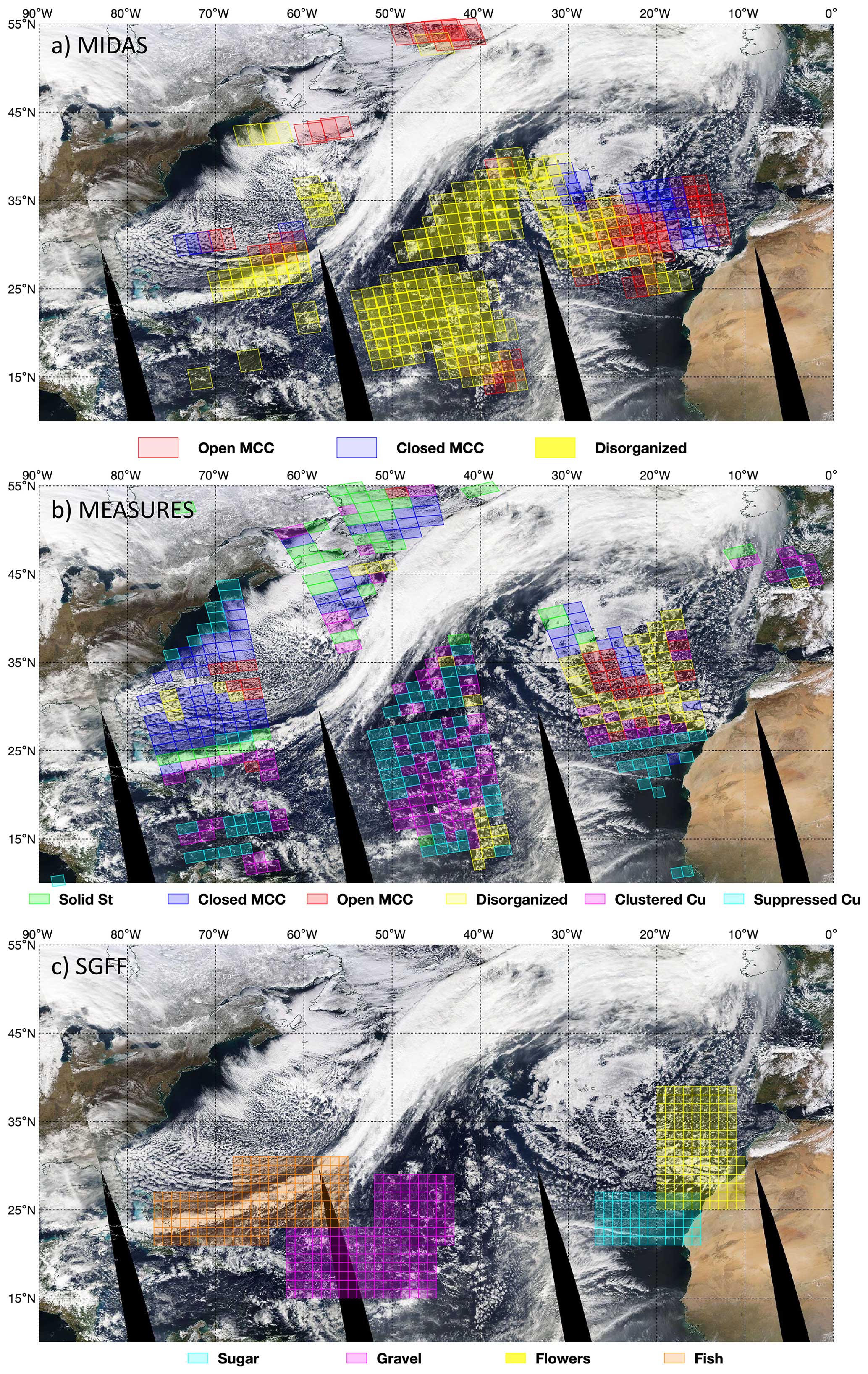
Figure 1The cloud field from 26 January 2018 with overlaid classifications by (a) MIDAS, (b) MEASURES, and (c) SGFF. Colors may deviate from the legend if boxes overlap or if background colors differ. Image credit: NASA and MODIS Aqua.
Clouds are unclassified in a few regions for a variety of reasons. If overlying ice clouds are present, Sun glint is interfering with the retrievals, or if the observed patterns do not adequately satisfy any of the criteria for any morphology, then these are left blank. Future work may be able to identify other morphologies or transitions in these gaps, but we restrict the analysis here to only boxes that are classified. Colors may deviate from the legend shown if boxes overlap (red overlapping yellow may appear orange) or if the background color of the image changes.
The frequencies of observations of each morphology and their geographic distributions are shown in Figs. 2–4, where contour maps show how frequently morphologies were classified within 5° × 5° latitude–longitude boxes. These are absolute frequencies not relative to each classifier. The grid is aggregated from 1° × 1° in order to show smoother contours, meaning each 1° × 1° box classified within a 5° × 5° grid box counts as a single observation.
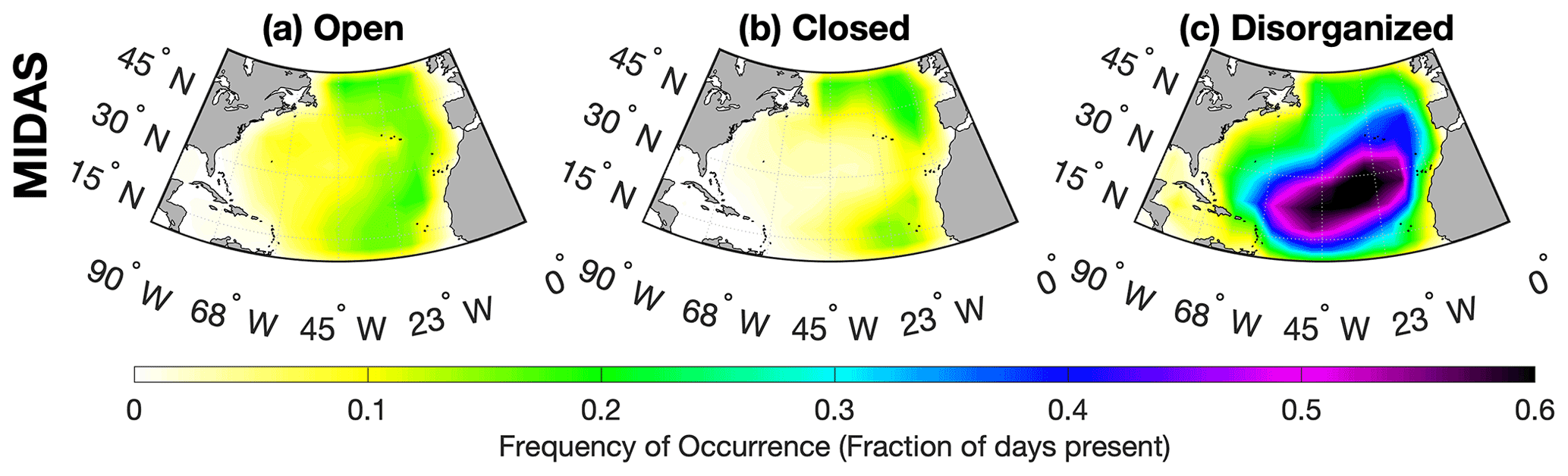
Figure 2The frequency of 1° × 1° grid boxes classified by MIDAS as (a) open MCC, (b) closed MCC, and (c) disorganized within 5° × 5° grid boxes.
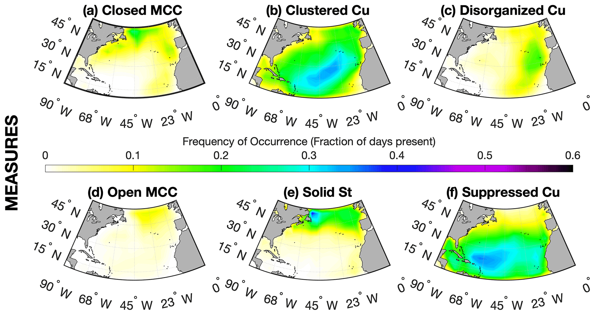
Figure 3The frequency of 1° × 1° grid boxes classified by MEASURES as (a) closed MCC, (b) clustered Cu, (c) disorganized Cu, (d) open MCC, (e) solid St, and (f) suppressed Cu within 5° × 5° grid boxes.
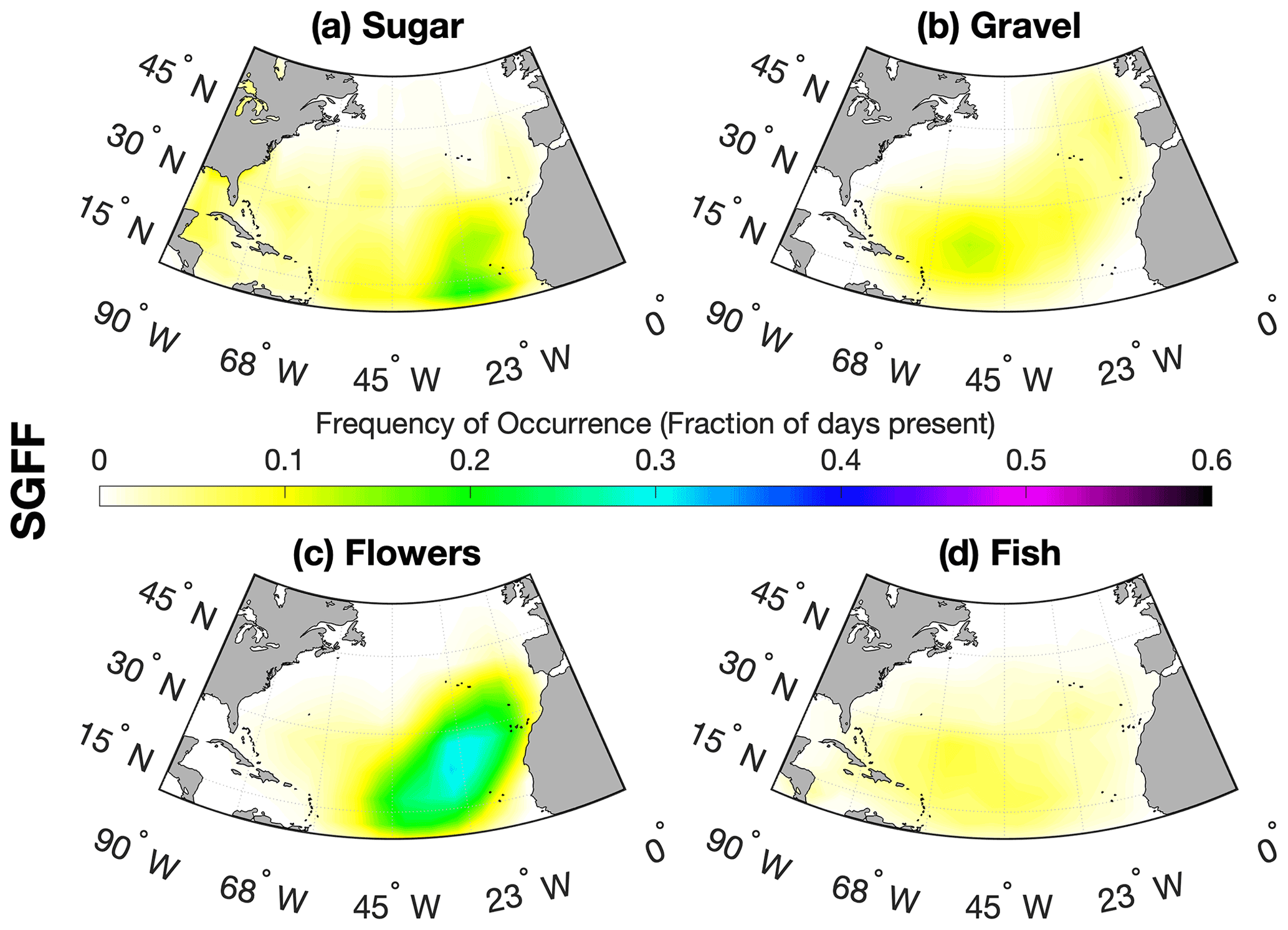
Figure 4The frequency of 1° × 1° grid boxes classified by SGFF as (a) sugar, (b) gravel, (c) flowers, and (d) fish within 5° × 5° grid boxes.
MIDAS open and MIDAS closed (Fig. 2) cells are observed less frequently than MIDAS disorganized and occur in roughly equal amounts in the mid-latitude storm track and subtropical subsidence region. MIDAS disorganized clouds are extremely common across the entire trade wind belt. This region experiences mean anticyclonic (clockwise) boundary layer wind flow centered over the central Atlantic (Brueck et al., 2015). The peaks in cloud-type distributions coincide with this flow. MIDAS closed MCC transition to MIDAS open MCC further downstream in the mid-latitude storm track and subsidence region. These transition into MIDAS disorganized scenes even further downstream as clouds are brought into the deeper tropics in the trade wind flow toward the Caribbean.
Figure 3 shows the distributions of MEASURES cloud types and adds specificity to the cloud transitions seen in MIDAS associated with the mean anticyclonic Atlantic winds. Furthest upstream in the cold-air-outbreak region, just offshore of the Canadian Maritimes, MEASURES solid St occurrence peaks. Downwind (eastward) of that peak are subsequent distribution peaks in MEASURES closed MCC, then MEASURES open MCC, followed by MEASURES disorganized clouds in the subsidence region offshore of western Europe. In contrast with the MIDAS routine, MEASURES closed and MEASURES open MCC are less frequent overall and are classified more frequently in the mid-latitude storm track compared to the subsidence region. MEASURES disorganized clouds are seen primarily in the eastern Atlantic. Rounding the eastern extreme of the North Atlantic high, MEASURES clustered Cu occurrence peaks first before MEASURES suppressed Cu, which dominates the downwind trade winds just upwind of the Caribbean. This distribution progression highlights the frequent Lagrangian morphology transitions that occur as air masses advect equatorward in the anticyclonic mean flow.
The geographical distributions of the SGFF morphologies are shown in Fig. 4 and mainly describe clouds near the tropical belt. Sugar is seen most frequently in the upstream trade winds off the coast of Africa, with a second region of frequent occurrence nearer the Caribbean. Gravel is most frequent just upstream of the Caribbean, downwind of the sugar maximum. Flowers are observed most frequently in a region spanning the subtropical subsidence region and upwind tropical belt, where Sc types are generally transitioning to more tropical Cu cloud types. This is consistent with the more stratiform nature of flowers, as observed by Schulz et al. (2021). These distributions suggest sugar cloud types can occur across the trade winds but may frequently form in offshore winds originating over Africa. It is likely these shallower Cu deepen into convective structures akin to gravel and flowers (Narenpitak et al., 2021) as they travel across the trade winds. Fish is the least frequently observed type and is most common in the south–central Atlantic. It should be noted that Schulz et al. (2021) also found sugar frequently occurring adjacent to the Inter-Tropical Convergence Zone (ITCZ) and its nearby subsidence region.
3.2 Co-occurrence statistics
To assess how the different routines classify the same scenes, Fig. 5 illustrates co-occurrence between the morphologies. A 1° × 1° grid box may have multiple classifications assigned by differing routines or from the same routine due to overlapping observation boxes or a box containing an “edge” between classifications. At the chosen resolution of the dataset, co-occurrences can stem from morphologies overlapping or being adjacent to each other within a box. Due to the patterns' mesoscale extent, this unresolved co-occurrence affects only the edges of the patterns and is assumed to have no affect on the geospatial analysis. To quantify co-occurrence, we show a fraction where the denominator is the total number of times a morphology represented on the x axis is classified, and the numerator is the number of times the two morphologies are observed in the same 1° × 1° box (same place; same time). Co-occurrence events are weighted by the surface area within grid boxes, so smaller grid boxes in the northern region contribute less to the frequency due to their relatively smaller surface areas. Differences between the co-occurrence fractions for elements above and below the central diagonal indicate differing frequencies of observations of one morphology (y axis) given the presence of the other (x axis).
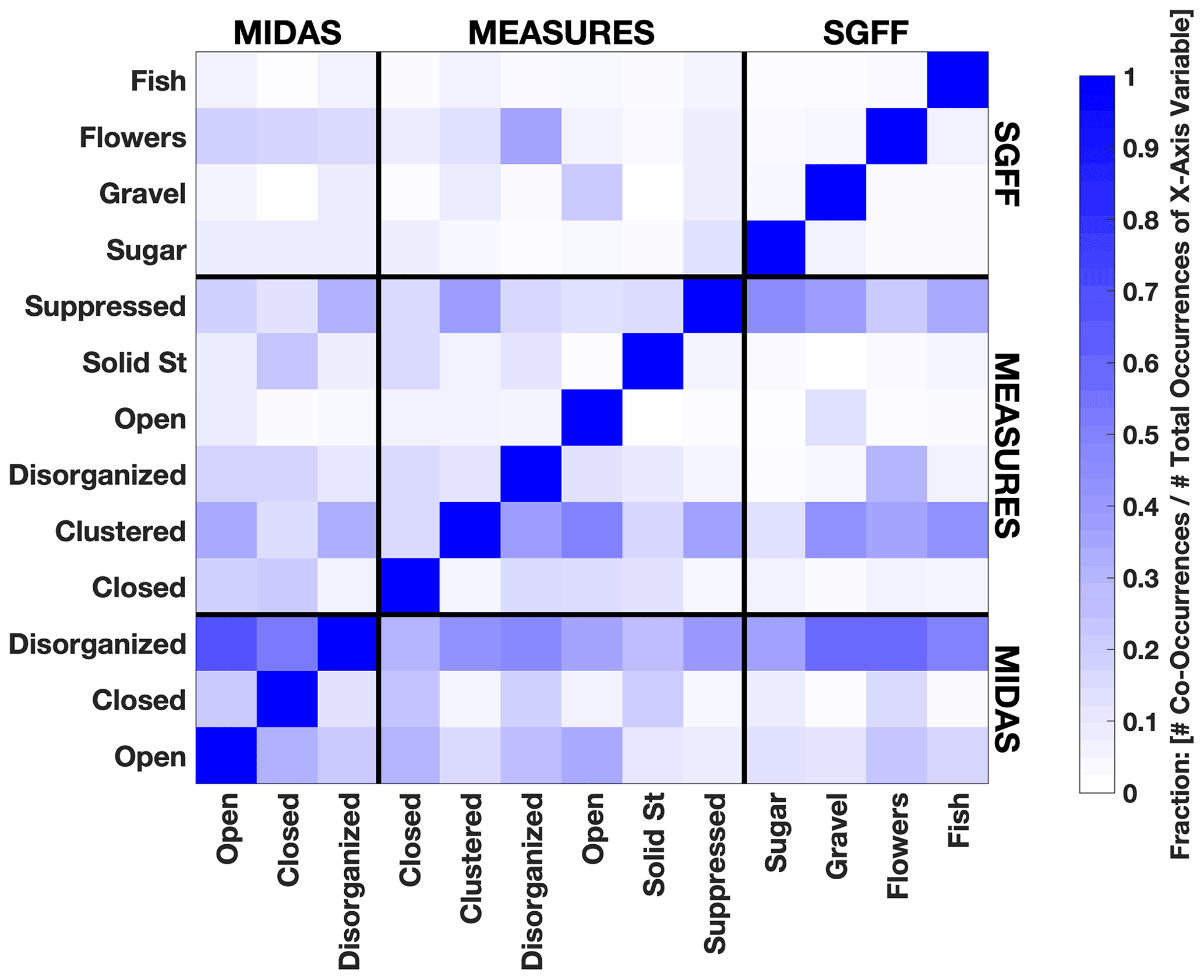
Figure 5Co-occurrences of cloud morphologies shown as a fraction. The numerator is the number of times the two morphologies are classified at the same place and same time, and the denominator is the total number of times the x-axis morphology is classified. Black lines separate classifier routines (labeled at top and right edge). Individual classification labels are marked along the bottom and left edge. Contributing boxes are area-weighted to account for varying grid box area with latitude.
The fractions of co-occurrence are shown as shades of blue in Fig. 5, with darker shades indicating more frequent co-occurrence. This representation allows us to compare scene classification behaviors within and between classifier routines (separated by black lines). MIDAS-classified scenes show the most within-routine overlap of any classifier examined, with MEASURES and SGFF coming second and third, respectively. The overlap sampling method of MIDAS scenes is likely responsible for this. Within MIDAS, MIDAS disorganized scenes overlap more with MIDAS closed or MIDAS open MCC relative to the less frequent overlap between MIDAS closed and MIDAS open MCC. This suggests that edges between MIDAS closed or MIDAS open MCC and MIDAS disorganized scenes are more common than edges between MIDAS closed and MIDAS open MCC. Between the MIDAS and MEASURES classifications, open MCC classifications frequently overlap, as do MIDAS closed MCC with MEASURES closed MCC and MEASURES solid St. This suggests a broad classification verification for these types between the MIDAS and MEASURES routines. MIDAS disorganized scenes have the most frequent overlap with other classification routine types, excluding MEASURES closed MCC, MEASURES solid St, and sugar.
MEASURES clustered scenes overlap with MEASURES open MCC and MEASURES suppressed Cu scenes. Taken together with the maps from the prior section, a Lagrangian model emerges, where MEASURES open cells evolve into sparser MEASURES clustered Cu, which then alternates with MEASURES suppressed Cu in the tropical trade winds. MEASURES clustered and MEASURES suppressed scenes overlap with MIDAS disorganized scenes, showing that the MEASURES routine accomplishes its mission of adding further detail to the expansive MIDAS disorganized classification. MEASURES clustered scenes overlap with gravel and fish, while MEASURES suppressed scenes overlap more with sugar, gravel, and fish. It is likely that MEASURES suppressed Cu is detected in gaps between larger features in fish and gravel scenes.
The SGFF classifications show less frequent overlap with one another, but some overlap is apparent between sugar–gravel and fish–flowers. Flowers overlap most with MIDAS open MCC and MIDAS disorganized, in addition to MEASURES clustered and MEASURES disorganized. Sugar and MEASURES suppressed Cu show some overlap, as do gravel and MEASURES clustered Cu, indicating that the two routines are classifying the same scenes as these conceptually similar types.
3.3 Morphology and albedo
In this section, we construct comparisons between various cloud properties for each morphology to understand the influence morphological organization has on albedo. Generally, we utilize one variable to define quantile bins along the x axis and report the mean of a second variable in each bin (e.g., shaded lines in Fig. 6). Grid box area is used to weight all averages shown, so smaller boxes do not have disproportionate contributions. The 2σ standard error for each bin mean is shown by the line width in the y direction. To eliminate noise caused by outliers, data plotted in the lines represent the middle 80 % quantile (with the upper and lower 10 % removed). Large, filled symbols represent the morphology mean x and y behavior. Small, hollow symbols mark the morphology corresponding to each line. We are able to examine inter-morphology (between mean morphology behaviors, comparing large symbols) relationships and intra-morphology (within morphology type behaviors, comparing shaded lines) relationships to test whether observed behaviors are unique to each type or common to all morphologies.
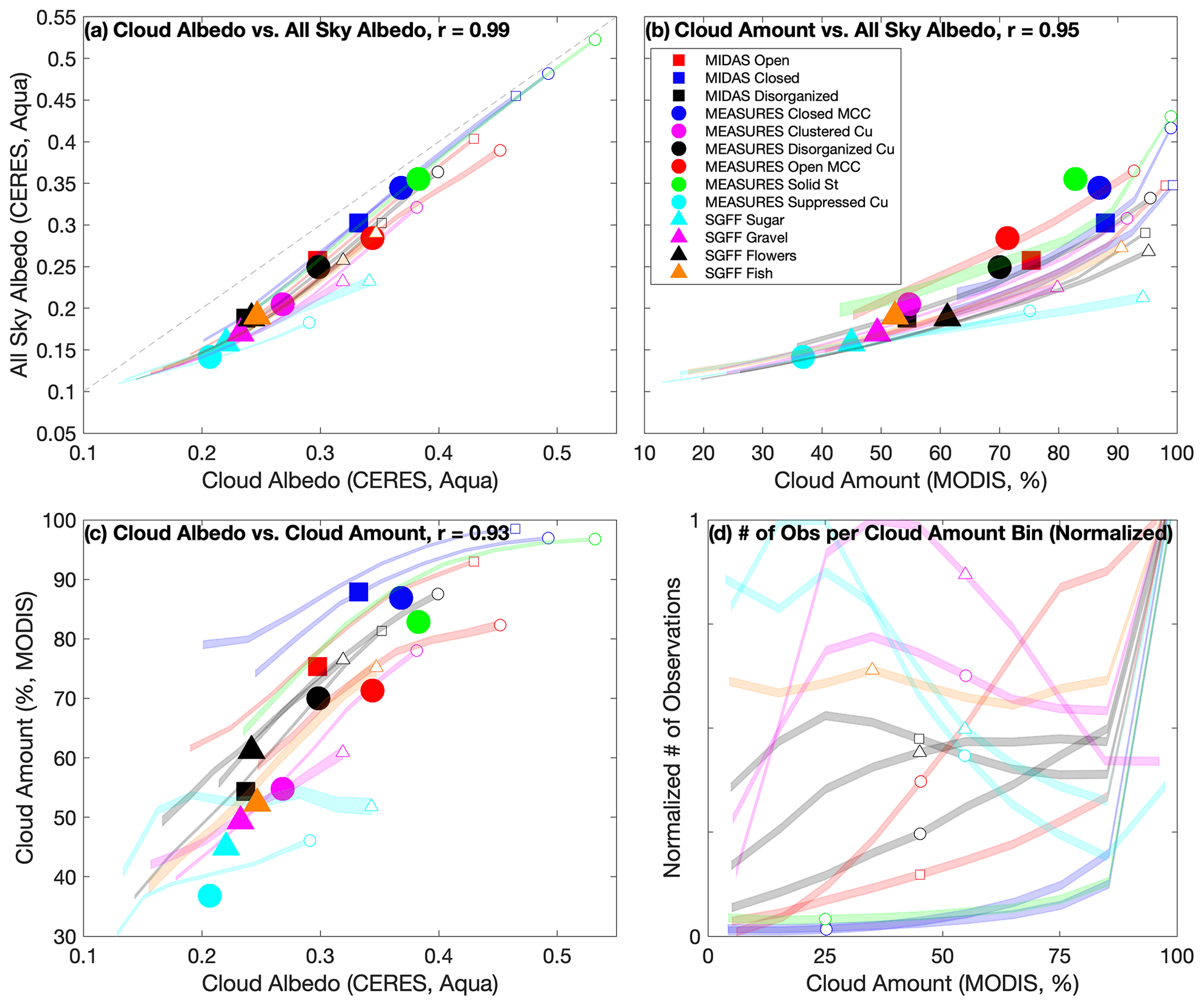
Figure 6Morphology relationships (colored lines) for y-axis variables binned into quantiles along the x axis between (a) cloud albedo vs. all-sky albedo, (b) cloud amount vs. all-sky albedo, (c) cloud albedo vs. cloud amount, and (d) cloud amount vs. normalized number of observations. Line width in the y direction represents the 2σ standard error of the mean. Data for lines exclude the upper and lower 10 % quantile bins. Hollow symbols and colors distinguish lines between classifier routine classifications (legend in (b)) and do not represent any values. In panels (a–c), averages for each morphology are shown as large, corresponding, and filled symbols. In panel (d), the observation number per cloud amount bin is normalized between 0–1 in order to best compare shape.
Each figure in this section has been produced using two methods; one uses all grid boxes assigned to a morphology, while the other uses a “pure” set that only uses boxes assigned to a single morphology by each routine (no co-occurrences within classifiers). This is to ensure that no bias is present due to overlap between morphologies. Figures are qualitatively identical regardless of which method is used and show no bias caused by overlap. Figures shown use all available data, including co-occurrences within classifiers.
For each morphology, we find that the scene (all-sky) albedo is both a function of cloud albedo (Fig. 6a) and cloud amount (Fig. 6b). The correlation coefficients shown are calculated for the means (large symbols) and describe how much variation between morphologies in mean scene albedo is explained by cloud albedo (Fig. 6a) and cloud cover (Fig. 6b). Cloud albedo explains slightly more (98 %) of the variability in all-sky albedo compared to cloud cover (90 %). Cloud amount and cloud albedo (Fig. 6c) are also closely related to each other with 86 % variance explained.
There is broad agreement in albedo values for similar cloud types seen by different classifiers. For example, MEASURES suppressed Cu and sugar show nearly equivalent albedos. Albedo tends to be lowest for Cu types and highest for stratiform types, with open cells, disorganized scenes, and clustered cumuliform albedos in the middle. Stratiform types show far more extensive cloud cover accompanied by a higher albedo compared with cumuliform types.
The spread between lines in the three plots suggests that the relationships between mean scene albedo and mean cloud amount, as well as between mean cloud albedo and mean cloud amount, are unique functions of cloud morphology. This is particularly true for the cloud albedo and cloud amount relationships, which exhibit more separation (Fig. 6c). For instance, the two suppressed Cu cloud types in Fig. 6c show a significantly less extensive mean cloud amount and a weaker increase in amount when albedo increases relative to stratiform morphologies. Differences are also present in Fig. 6a, where, again, the suppressed Cu types show a weaker relationship along with gravel and MEASURES open cells. Taken together, these figures show how mean radiative properties for each cloud morphology are a unique function of cloud cover and cloud albedo.
Table 1Correlations between all-sky albedo and cloud albedo (first column) and between all-sky albedo and cloud amount (second column) for each morphology.
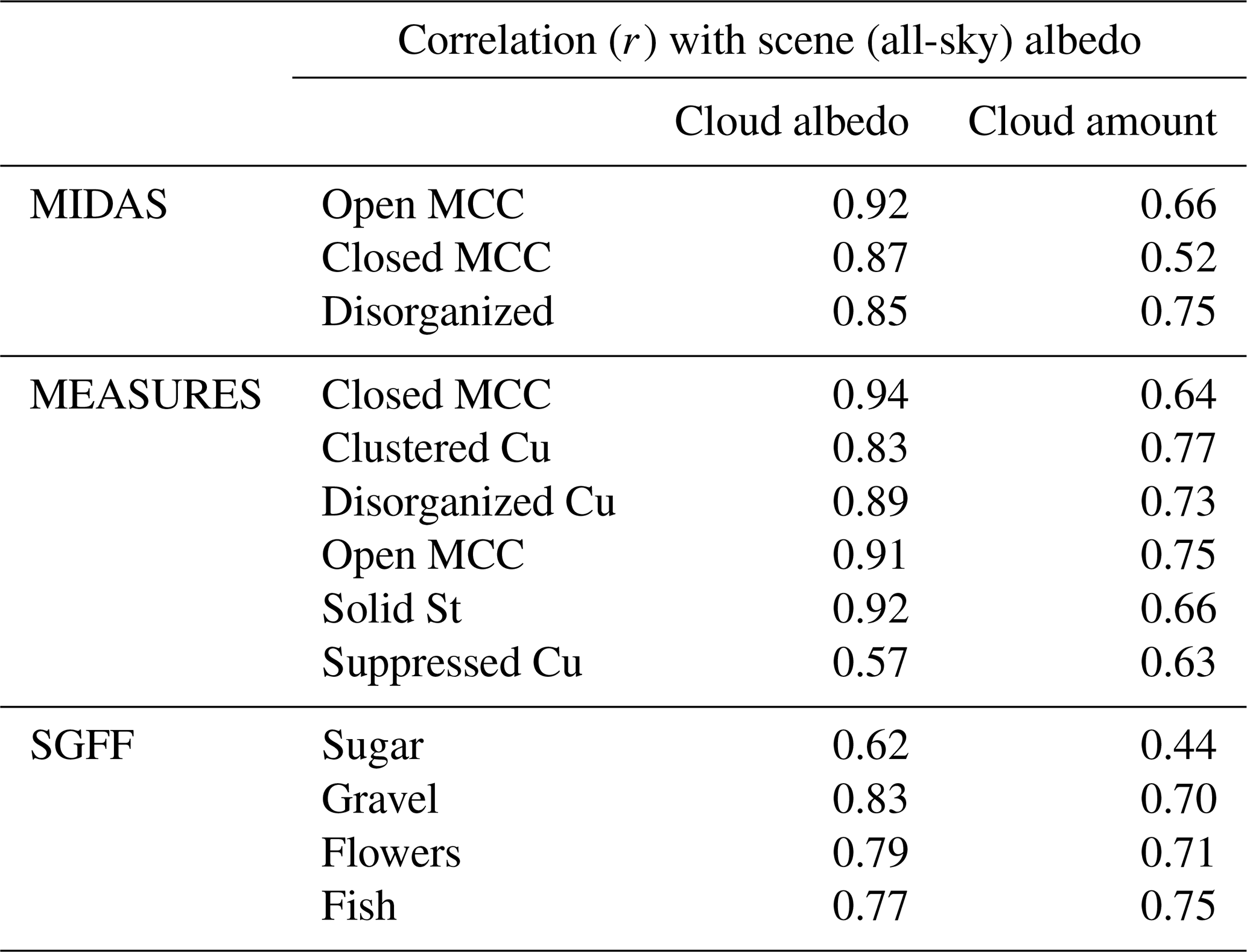
In addition to the correlations between the mean morphology behaviors, we examine the correlations based on the points used to create the shaded lines in Fig. 6a–c. These coefficients (Table 1) describe how strongly cloud albedo or cloud amount relate to scene albedo for each morphology. For every morphology (with the exception of MEASURES suppressed), cloud albedo is a stronger driver of scene albedo than cloud cover. This is consistent with the mean correlations and implies that, for these morphologies, cloud reflectivity may drive all-sky albedo variability more strongly than cloud amount. These relationships are generally weaker for the suppressed Cu types, which may indicate the difficulty in detecting the larger proportion of optically thin clouds in these predominantly clear scenes (Mieslinger et al., 2022).
Figure 6d shows normalized curves comparing the relative number of observations per cloud amount bin for each morphology. These curves show that stratiform types are more frequently observed in cloudy environments, while most of the disorganized or cumuliform types are frequently observed when cloud cover is much lower. However, the distribution of morphology occurrence across the cloud amount space is varied and overlapping, suggesting that morphology is not a simple function of cloud cover, or vice versa.
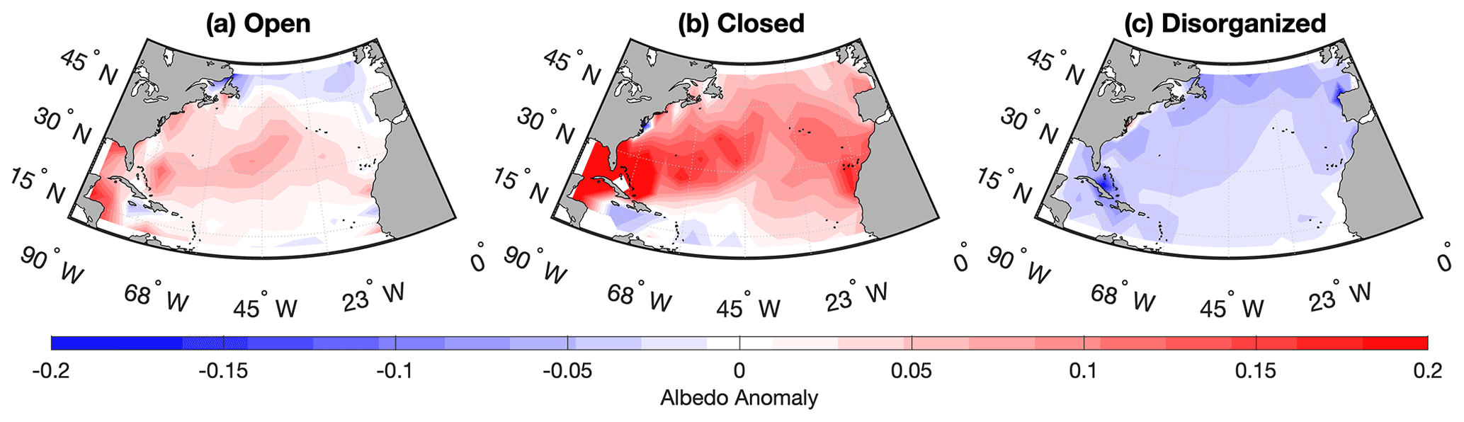
Figure 7Yearly mean of daily albedo anomalies relative to the 100 d running mean for all classifiable low-cloud scenes for MIDAS morphologies: (a) open MCC, (b) closed MCC, and (c) disorganized.
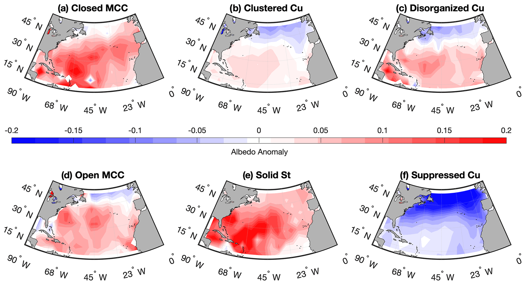
Figure 8As in Fig. 7 but for MEASURES morphologies: (a) closed MCC, (b) clustered Cu, (c) disorganized Cu, (d) open MCC, (e) solid St, and (f) suppressed cu.
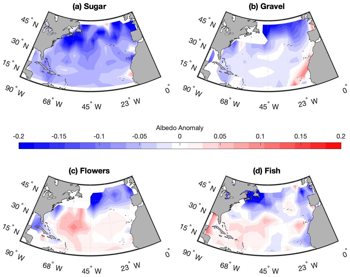
In Figs. 7–9, maps show the geographic distributions of cloud albedo anomaly for each morphology. Albedo anomaly is defined as the daily mean albedo for a specific morphology minus the mean albedo for all sampled low-cloud scenes (from a combination of all routines) within a 5° × 5° grid box for a 100 d running mean centered on every day. The values shown are annual means. Results show that MEASURES suppressed Cu, sugar, gravel, and MIDAS disorganized scenes have anomalously low albedos throughout our region, while closed-cell Sc and solid stratiform clouds almost always have anomalously high albedos. For other types, including MIDAS open cells, MEASURES open cells, MEASURES clustered, MEASURES disorganized Cu, fish, and flowers, the albedo anomaly is negative near the storm track but positive to the south. This suggests a complex picture where climatologically relevant cloud radiative properties are a function of morphology and location. Because of differing frequencies of occurrence for each morphology (as shown in Figs. 2–4), the sum of all anomalies in Figs. 7-9 should not be zero.
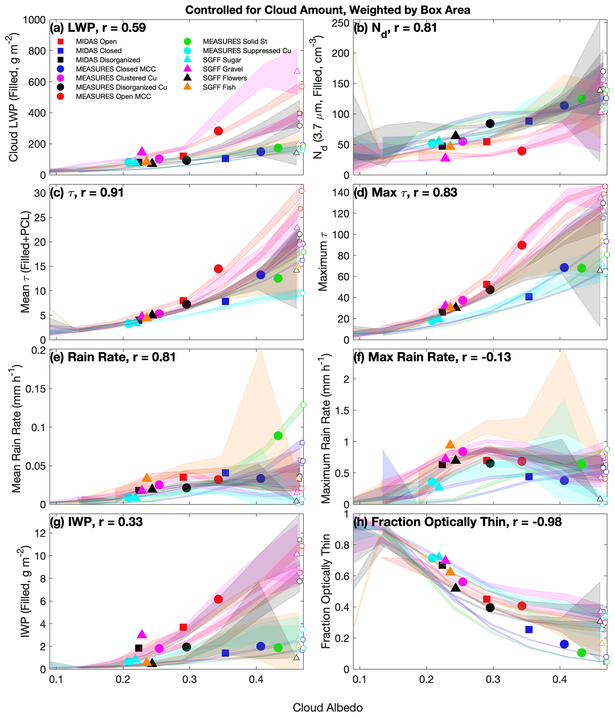
Figure 10Cloud properties: (a) in-cloud liquid water path (LWP), (b) droplet number concentration (Nd), (c) mean optical depth (τ), (d) maximum optical depth, (e) mean rain rate, (f) maximum rain rate, (g) in-cloud ice water path (IWP), and (h) fraction of optically thin cloud features (τ<3) as a function of cloud albedo. As in Fig. 6, symbols show the mean relationship for each classification, lines show the relationship for cloud properties within each morphology for bins of constant cloud albedo, and line width in the y direction represents the 2σ standard error of the mean. Panels (a), (b), and (g) only use Filled MODIS pixels and not cloud edges in order to reduce possible biases in retrievals in partly cloudy regions.
In Fig. 6 and Table 1, cloud albedo was shown to have a stronger effect than cloud amount on the all-sky albedo of a cloud scene. This motivates further study into which cloud properties most influence cloud albedo for each morphology. In Fig. 10, the relationships between cloud albedo and a number of remotely sensed cloud variables are shown for each morphology using the same method as Fig. 6. Data are gathered only for cloud scenes with cloud amounts within 10 % of the respective morphology median, which allows us to control for the differing mean cloud amounts associated with the morphologies (sampling the “peaks” relative to cloud amount in Fig. 6d). Results were not qualitatively sensitive to changing this threshold to 5 % or 20 %.
For all morphologies, cloud albedo increases when LWP, Nd, τ, and IWP (Fig. 10a–c and g, respectively) increase, while cloud albedo decreases when the fraction of optically thin cloud cover increases (Fig. 10h). This final relationship shows the strongest correlation, indicating that the fraction of optically thin cloud cover most strongly explains the cloud albedo variability between morphologies after controlling for cloud amount, as shown by McCoy et al. (2023).
Figure 10 uses LWP, Nd, and IWP values from Filled MODIS pixels only, excluding cloud edges or any other scenes where pixels are partially filled. This is to avoid biases caused by assumptions used by the retrievals that may not be appropriate in broken cloud scenes. To see whether including or excluding broken scenes could cause a bias, Fig. 10 was also produced using weighted averages of Filled and PCL pixels, with separate LWP, Nd, and IWP values averaged for portions of each grid box considered Filled or PCL and then averaged based on the fraction of Filled or PCL scenes within each box. This averaged figure was qualitatively unchanged from the original, suggesting that the relationships seen here are unlikely to be biased by scattered or broken cloud scenes. Optical depth values use this weighted-average technique, incorporating Filled and PCL observations, since that product relies on fewer assumptions.
The spread of lines in the y direction in Fig. 10 indicates that there is some degree of cloud albedo equifinality across morphologies. That is, different morphologies can produce an equivalent cloud albedo despite significantly different cloud properties. A comparison of the plotted lines shows that more cumuliform morphologies such as gravel, disorganized clouds, and open-cell MCC have higher values of maximum τ, higher peak rain rates, more ice content, and more optically thin clouds compared to the stratiform types for an equivalent cloud albedo. This suggests that the cumuliform morphologies are characterized by thick raining cores surrounded by optically thin clouds while stratiform morphologies are much more uniform.
We find a curious difference when comparing mean τ and peak τ versus comparing mean rain rate and peak rain rate behaviors. The relationship between τ and cloud albedo is consistent and positive for both mean and maximum τ (Fig. 10c and d). However this is not the case for rain rates; mean rain rates are higher for a higher albedo, but maximum rain rates are highest for middling albedos over a broad set of cumuliform morphologies. This nuanced relationship between maximum rain rate and albedo may be associated with heavily precipitating cores surrounded by more optically thin clouds. Because of the limitations in the 89 GHz rain rate product in sensing heavier rain, this result may need to be evaluated using rain rate products with a greater sensitivity to strong rain rates.
3.4 Vertical profiles and optical thickness from CALIPSO
The CALIOP lidar aboard CALIPSO provides vertical profiles of cloud tops and a measure of cloud optical thickness. This section analyses cloudy retrievals in 30 m height bins in the lowest 4 km of CALIOP lidar profiles in classified boxes. Profiles that penetrate the clouds and detect the surface are considered optically thin, while fully attenuated profiles are considered optically thick. Optically thick profiles only represent cloud tops, since the true vertical extent of the cloud is unknown due to attenuation of the lidar beam. Profiles that see layered clouds are more complex; occasionally, the lidar sees through upper clouds and attenuates in a lower cloud. Here, layered profiles are split into thin and thick portions. The thin portion represents all clouds that the lidar sees through, and the thick portion consists only of the cloud that fully attenuates the beam. Plots in Fig. 11 show the fraction of cloudy observations for thin (dashed blue) and thick (solid black) profiles in each height bin divided by the total number of profiles that see cloud for each classification. Combined profiles (sum of thick and thin) are shown as dashed thin black lines. Clear profiles are excluded from the denominator in order to better show and compare the shapes of the cloud profiles. Anomalies for thin and thick profiles, shown, respectively, as shaded blue and black regions, represent the profiles for each type minus the mean profile of all types shown in Fig. 11n. Frames are arranged to facilitate comparisons between theoretically similar identification types across classifiers.
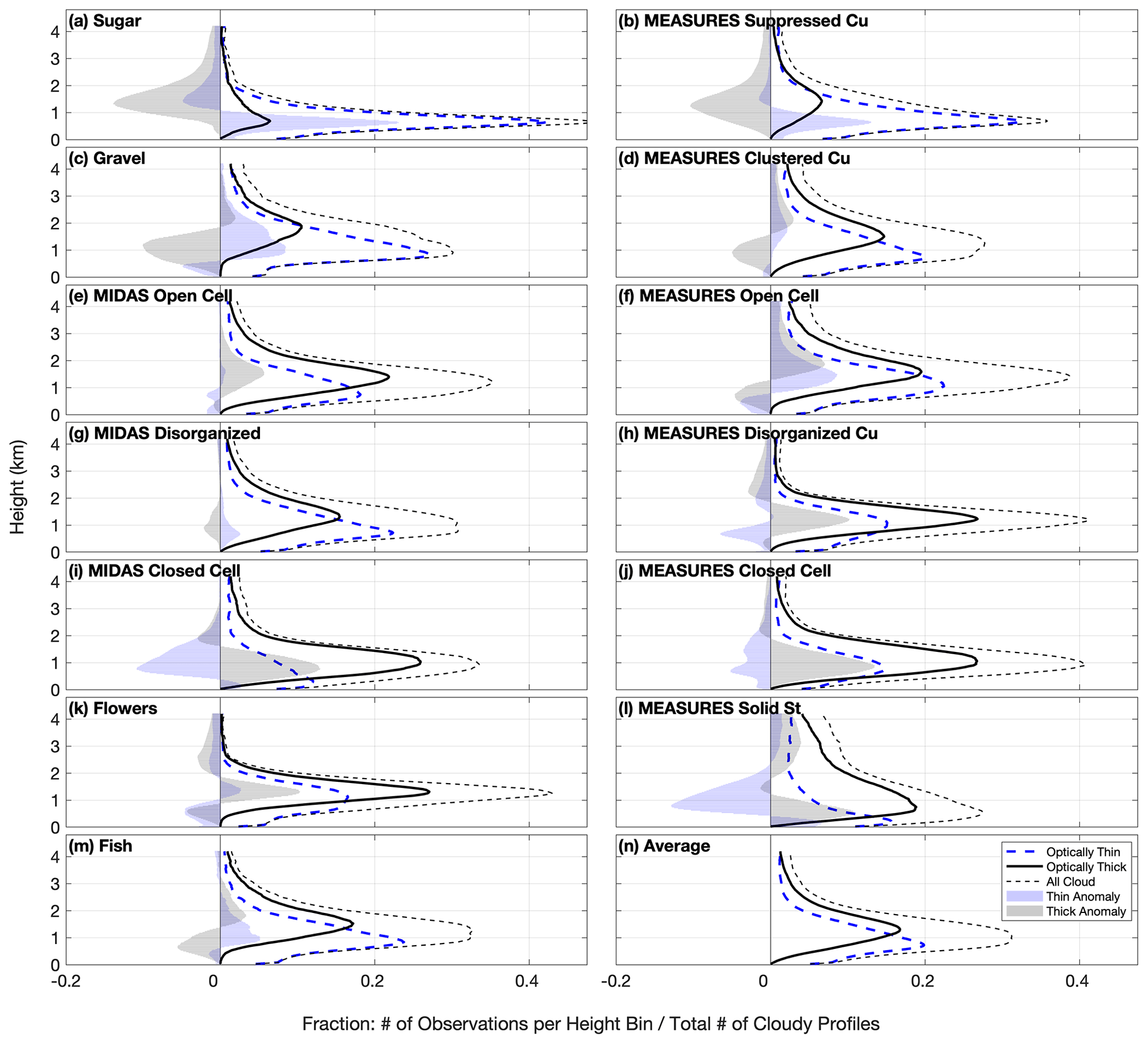
Figure 11CALIPSO vertical feature mask (VFM) vertical profiles of all (dashed black), optically thin (dashed blue), and thick (solid black) clouds for each morphology. Anomalies relative to the mean profiles in panel (n) are shown as shaded regions (blue for thin; black for thick).
Since overlying high clouds could potentially attenuate the lidar beam, Fig. 11 was also created only for profiles with no cloud cover above 4 km. This filtered subset of our data produced qualitatively comparable results and showed no bias caused by high clouds.
Results show strong differences in vertical profiles between classifications. Shallower and less vertically distributed types include suppressed Cu types, closed MCC, MEASURES disorganized, and flowers. Deeper types are gravel, open cells, MEASURES solid St, and fish. These deeper types tend to rain more heavily (Fig. 10f), except for MEASURES solid St which are likely associated with weather systems and not convection. Note that because we are limiting to 4 km depth, the fish identifications are likely highlighting the low-level scud clouds that happen in the vicinity of the larger feature (e.g., Fig. 1). Generally, optically thin clouds tend to be lower in height than surrounding optically thick clouds for all classifications even when accounting for layered scenes.
Comparing absolute and anomaly profiles between similar types classified by different routines, we find similar behaviors for suppressed Cu types (MEASURES suppressed vs. sugar) and closed MCC types (MEASURES vs. MIDAS). Some differences are apparent between other theoretically similar types. Gravel scenes tend to contain more optically thin and fewer optically thick clouds compared to MEASURES clustered Cu. This may be because more optically thin clouds are present in the larger classification boxes around gravel. MEASURES open cells contain more clouds, especially optically thin, in the upper portions of the profile compared to MIDAS open cells, perhaps owing to the MEASURES open cells' disproportionate prevalence in the storm track.
CALIOP provides an independent measure of the fraction of optically thin clouds that can be compared to MODIS. In Fig. 12 the number of CALIOP profiles that see the surface divided by the total number of cloudy profiles is plotted against the fraction of cloudy MODIS pixels with τ<3. Layered CALIOP soundings are considered optically thick here, since an equivalent MODIS observation would be unable to effectively distinguish the layers, and the albedo would be more akin to that of an optically thick scene. We see strong agreement between MODIS and CALIOP measures of τ (88 % variance explained), increasing confidence in our assessment of optically thin fractions for the classified types.
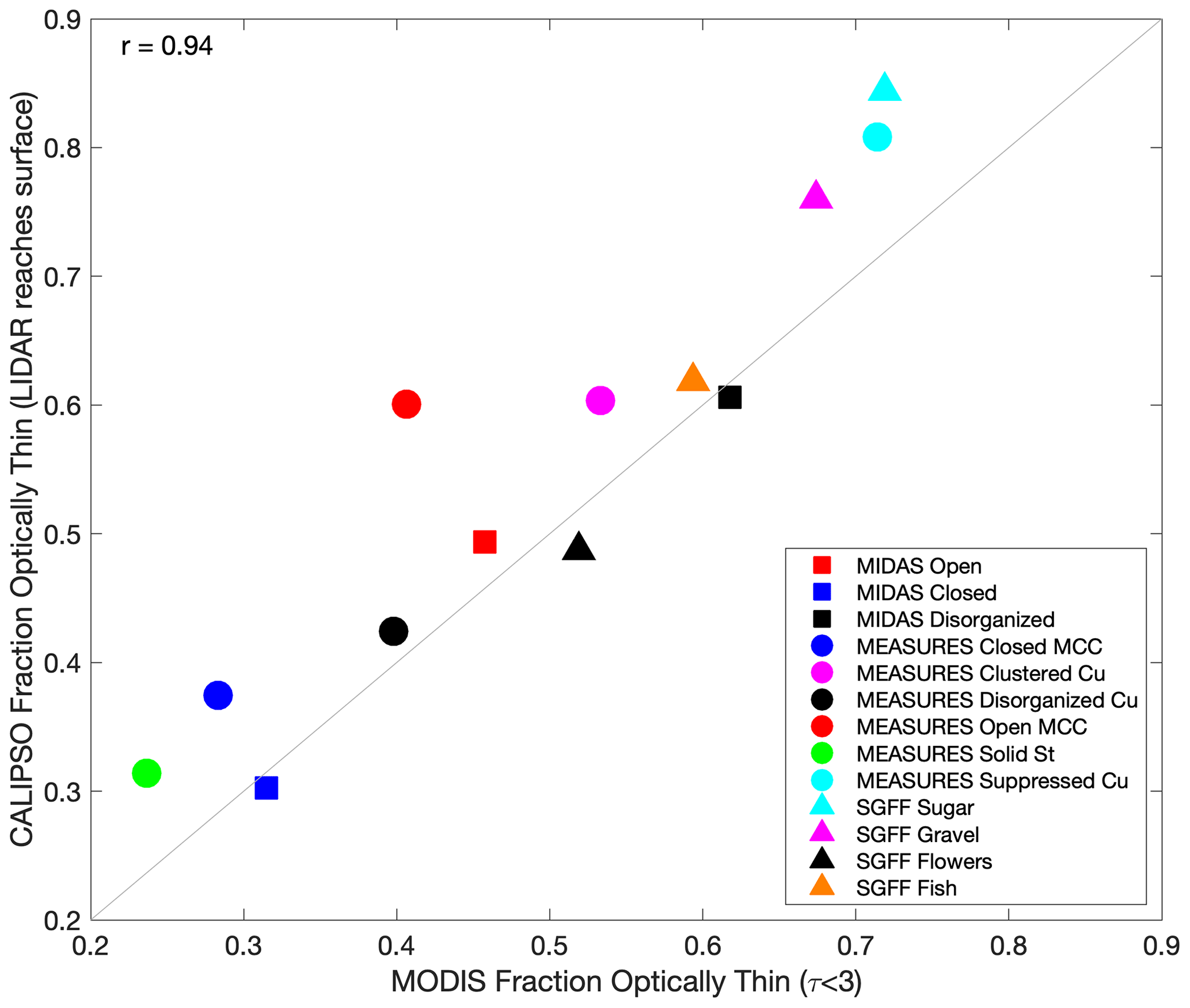
Figure 12Mean optically thin cloud cover fraction as detected by MODIS (no. of observations with τ<3 divided by the total no. of cloudy observations) plotted against mean optically thin cloud cover as detected by CALIOP on CALIPSO (no. of soundings that see the surface divided by the total no. of cloudy soundings).
3.5 Regional differences
Figure 10 shows significant differences in cloud properties between morphologies, while Figs. 2–4 show strong differences in their geographic distributions. Given this, we wish to investigate the degree to which cloud property differences are influenced by varying geographic distributions separately from morphological differences. To assess this, Figs. 14 and 15 present a comparison of cloud properties in smaller sub-regions that are illustrated in Fig. 13. Boxes sample different sub-regions along the anticyclonic flow in the Atlantic, as illustrated by mean winds at cloud level (vectors; 925 hPa). Boxes in the far North Atlantic and East Atlantic subsidence regions are chosen to compare stratiform morphologies, while boxes in the upwind and downwind tropical trade winds are chosen in order to compare shallow tropical convective morphologies. Plots compare cloud micro- and macro-physics, radiative properties, precipitation, and phase. Scatterplots in Figs. 14 and 15 present each sub-region on an axis. A 1:1 line is also shown, where the area-wide North Atlantic mean values for each morphology are shown as a hollow symbol in order to compare sub-regional behavior to the entire regional mean.
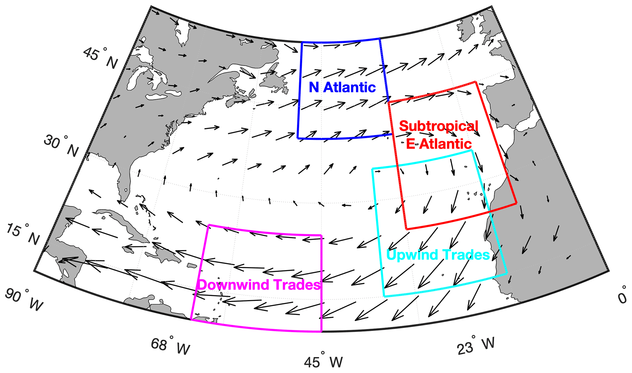
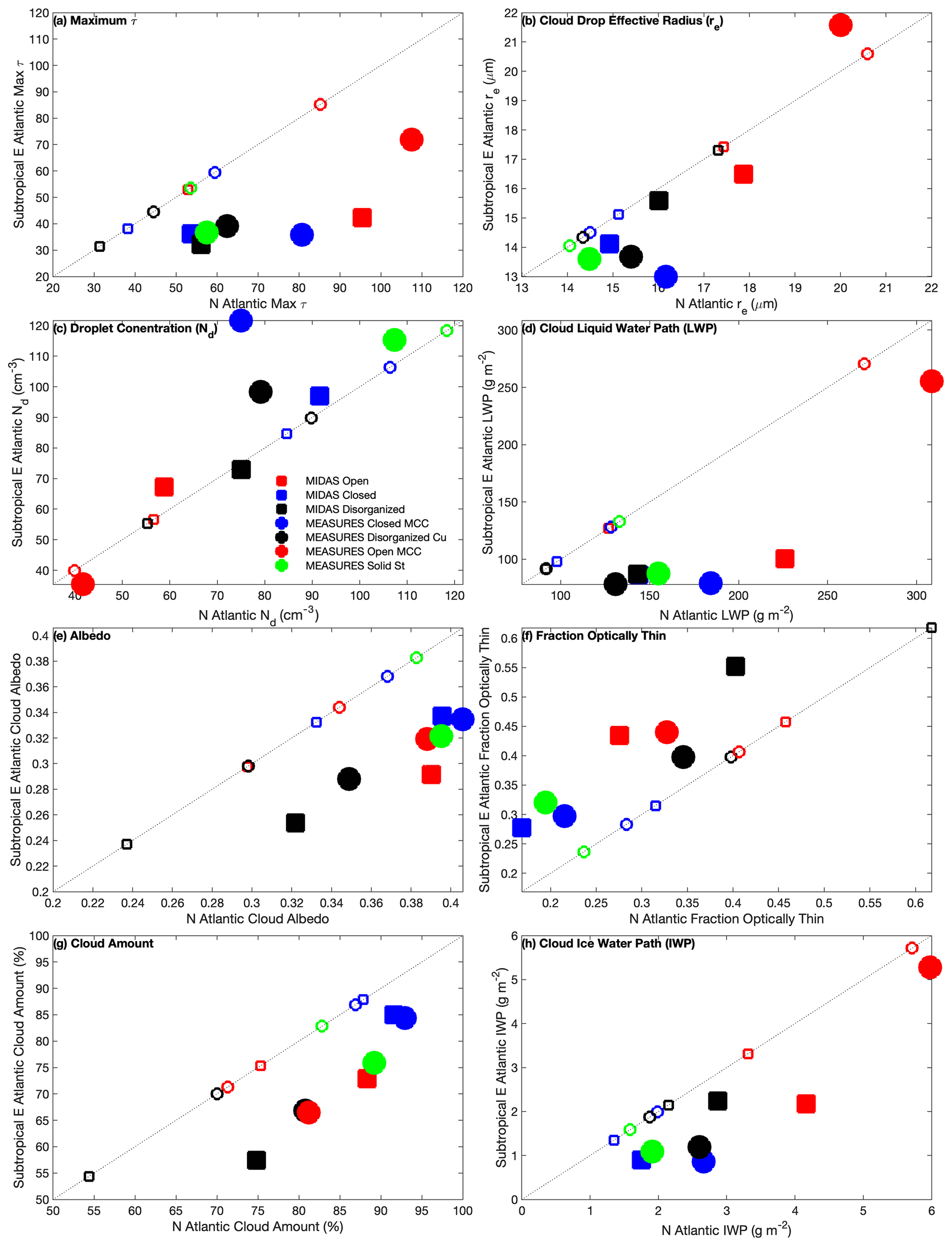
Figure 14Mean cloud properties for each morphology that is commonly observed in the far North Atlantic (x axis) and subtropical subsidence region (y axis). Properties include (a) maximum optical depth (τ), (b) cloud droplet effective radius (re; in place of rain rate), (c) cloud droplet concentration (Nd), (d) in-cloud liquid water path (LWP), (e) albedo, (f) fraction of optically thin cloud (τ<3), (g) cloud amount, and (h) in-cloud ice water path. A 1:1 line is also shown, where the area-wide North Atlantic mean values for each morphology are shown as a hollow symbol.
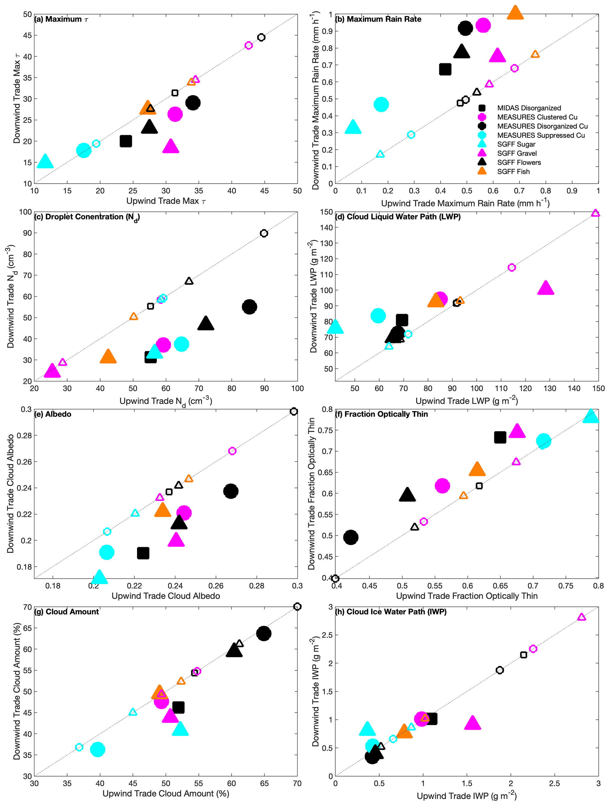
Figure 15Mean cloud properties for each morphology that is commonly observed in the far upwind trade winds (x axis) and downwind trade winds (y axis). Properties include (a) maximum optical depth (τ), (b) rain rate, (c) cloud droplet concentration (Nd), (d) in-cloud liquid water path (LWP), (e) albedo, (f) fraction of optically thin cloud (τ<3), (g) cloud amount, and (h) in-cloud ice water path. A 1:1 line is also shown, where the area-wide North Atlantic mean values for each morphology are shown as a hollow symbol.
Figure 14 compares the far North Atlantic with the East Atlantic subsidence region. This effectively contrasts stratiform morphologies between those that frequently occur in the storm track where cold air outbreaks are common and the Sc cloud types that commonly occur under a shallow marine inversion. Rain rate data derived from Tb are frequently missing in the far North Atlantic region due to the presence of ice, so rain rates are replaced by cloud droplet effective radius (re) in order to better compare rain characteristics. The far North Atlantic shows a greater maximum τ, marginally fewer but somewhat bigger cloud drops (likely indicating more rain), greater LWP and IWP, and more cloud cover but fewer optically thin clouds. These differences suggest a thicker, icier, and rainier cloud environment for all morphologies in the far North Atlantic. As a consequence of these thicker clouds, the cloud albedo in this region is consistently higher compared to both the entire study region and the subsidence region in the East Atlantic.
Figure 15 compares warm, shallow convective morphologies between upwind and downwind locations in the tropical trade winds (note axes changes from Fig. 14). Morphologies observed upwind have lower peak rain rates with more drops and are marginally cloudier with a smaller proportion of optically thin clouds. The cloud LWP is also marginally lower upwind, while ice is minimal in both sub-regions (not unexpected for the trades). The upwind region shows a higher max τ and albedo, suggesting that the cleaner (lower Nd), more remote, and likely more developed downwind cloud systems are less reflective. This result hints at the presence of strong Lagrangian development of cloud systems in the trade winds, which may have significant radiative implications.
Figures 14 and 15 show that the ordering from high to low for most cloud properties generally remains consistent between types and between regions, even though mean values may differ significantly between regions. Some of the variability seen in Fig. 10 is likely caused by geographic differences, but a strong morphology-driven variation in cloud properties is still present after controlling for regionality. Furthermore, Lagrangian development is apparent when looking at upwind/downwind locations in the trade winds. Finally, the association between rain rates and albedo may be dependent upon morphology or cloud phase, with more heavily raining warm tropical clouds being less reflective, while rainier, and possibly icier, scenes in the mid-latitudes have a higher albedo.
In Fig. 6 and Table 1, we show that cloud albedo is at least as strong a predictor of scene albedo as cloud amount. This was true in explaining albedo variability between morphologies (Fig. 6) and within morphologies (Table 1). Figure 10 goes on to show that the fraction of optically thin cloud cover best predicts the cloud albedo variability between morphologies, highlighting the importance of cloud optical thickness in climate studies. This result agrees with the results of McCoy et al. (2023) in showing that differences in cloud optical thickness between MIDAS morphologies drive albedo variation between those morphologies for a constant cloud amount. Here, we can now extend that conclusion by examining more specialized tropical cloud morphology identifications that were previously considered together as one disorganized type.
The relative importance of albedo and cloud cover in diagnosing the radiative impact of clouds is in part dependent upon thresholds used in satellite retrievals to identify cloudy or clear scenes. It is possible that a modification of the threshold used to separate cloudy from clear pixels in the MODIS cloud mask employed here could modify our results. Because no perfect truth exists for quantifying satellite-detected clouds, we motivate future work in this area to improve the resolution of cloud cover retrievals.
The radiative importance of cloud optical depth in our present and future climate has been demonstrated in prior work (McCoy et al., 2023; Hu and Stamnes, 2000; Konsta et al., 2022). Using a radiative–convective model, Hu and Stamnes (2000) found that an increase in cloud optical depth was associated with less warming. McCoy et al. (2023) used present-day morphology observations as a basis for calculating the optical depth component of the shortwave cloud feedback (e.g., Zelinka et al., 2012) from shifts in morphology occurrence under extreme climate scenarios. For example, McCoy et al. (2023) show a local, positive optical depth feedback on SST warming from morphology shifts, which occurred during the 2015–2016 North East Pacific marine heatwave; MIDAS-closed-cell MCC was replaced by less cloudy, optically thinner MIDAS disorganized scenes, increasing sunlight on the sea surface. Here, we expanded the specificity of morphology identifications, especially in the tropics, from those used in McCoy et al. (2023) and found some additional variation in behaviors across morphology types. Our results highlight the potential complexity of understanding morphology feedback onto the climate system in present and future climates. Identifying the processes involved in development and transitions across these varied morphology types and the sensitivity of these processes to the environment warrants additional study as well.
A comparison of climate models by Konsta et al. (2022) shows that models fail to reproduce realistic cloud optical depth variability, often producing no optically thin clouds. This contributes to the “too few, too bright” problem endemic in cloud representation in general circulation models. That study also showed a model failure to reproduce higher cloud optical depths observed in thicker Sc scenes. Examining parameterized cloud behaviors in the context of morphological classifications may aid in the reproduction of realistic optical thicknesses. Relating morphology occurrence, and their inherent radiative property signatures, to distinct climate regimes (e.g., McCoy et al., 2017; Mohrmann et al., 2021; McCoy et al., 2023) may also be useful in adding nuance to regime-based forcing (e.g., Wall et al., 2022) and feedback (e.g., Myers et al., 2021; Zelinka et al., 2022) calculations. In particular, trade–cumulus feedback is still a large source of uncertainty in climate models and significantly disagrees with observational estimates (e.g., Myers et al., 2021; Vogel et al., 2022), emphasizing the importance of understanding cloud development and radiative impacts in this region.
Geographic distribution maps and co-occurrence statistics shown in sections 3.1 and 3.2 suggest that Lagrangian transitions between morphologies are common as the mean flow advects clockwise (anti-cyclonically) around the study region. Given the regional morphology albedo anomalies we found (Figs. 7–9), Earth's radiation budget will be modified by shifts in the location of the climatological average transition regions or other changes in the most common types of transitions occurring in this basin. A few studies have already addressed the drivers of Lagrangian morphology changes in these regions. Narenpitak et al. (2021) demonstrated that moisture convergence and large-scale ascent can drive a sugar–flowers transition in the trade winds. Eastman et al. (2022) found that increased rain driven by strong winds and its accompanying moisture fluxes can drive a closed- to open-MCC transition in the subtropics, while a warmer sea surface, a weaker inversion, and stronger dry air entrainment were associated with MIDAS closed to MIDAS disorganized transitions. Identifying more such mechanisms influencing climatological and Lagrangian morphology transitions and their sensitivity to environmental changes will be important for understanding how these transitions will modulate present and future energy flows in the climate system.
Our results also motivate future work examining other frequent, radiatively significant transitions that are now apparent from the relatively frequent co-occurrences suggested in Fig. 5. For example, the change between disorganized types and flowers or suppressed Cu evolving into or from clustered Cu. The importance of examining these regionally specific transitions is further emphasized by our finding that a single morphology may present differing radiative characteristics as it undergoes Lagrangian evolution (e.g., along the flow), as shown by MEASURES clustered Cu or gravel becoming rainier and increasingly optically thin in the downwind trades (Fig. 15). That relationship combined with the heavier maximum rain rates observed at middling cloud albedo values in Fig. 10f for several shallow convective morphologies hints at a precipitation-driven process, where heavy rain may be associated with less reflective clouds for some morphologies. This may be broadly consistent with the increased prevalence of cloud-free cold pools surrounding mature raining cells. However, Vogel et al. (2021) suggest the opposite relationship with greater optical thickness associated with stronger rain rates. Heavier precipitation observed in the stratocumulus–cumulus transition was shown by O et al. (2018) to be associated with more optically thin veil clouds, which is broadly consistent with lower albedos seen with heavier rain rates. Further work is needed to better understand these processes. The differences in droplet concentrations (e.g., higher upwind in the trades) in Figs. 14 and 15 also motivate a more detailed examination of aerosol influence on morphology radiative properties (e.g., higher albedo upwind) and cloud evolution.
In Leahy et al. (2012), the fraction of optically thin cloud cover was shown to vary inversely with cloud size. Although our study has not specifically studied the sizes of cloudy elements within each morphology, our results generally agree with this inverse relationship. Morphologies such as MEASURES suppressed Cu or sugar, which consist of many small clouds, contain a greater proportion of optically thin cloud compared to the broad cells associated with closed-cell Sc. Objective classification methods have also found that cloud size is one of four important dimensions to consider in separating cloud morphology types, indicating this is a fundamental property of different organization states (Janssens et al., 2021). This motivates future study of cell size, possibly using methods developed by Zhou et al. (2021) and Janssens et al. (2021), to see whether this inverse relationship applies within each morphology or only between morphologies. Both Leahy et al. (2012) and Mieslinger et al. (2022) found that small, optically thin clouds are frequently undetected by remote platforms such as MODIS and CALIPSO, causing significant uncertainty in cloud radiative effects and suggesting that optically thin fractions shown here may be underestimated. Advances in observations may aid in detecting these “hidden” but radiatively significant clouds.
In Fig. 5, open-cell co-occurrence statistics are peculiar in that MEASURES open cells tend be infrequent when MIDAS open cells are reported, relative to the opposite relationship where MIDAS open cells are more frequent when MEASURES open cells are present. Differing geographic distributions are also present in Figs. 2a and 3d, showing that MEASURES open cells are more confined to the storm track where Fig. 15d shows much higher LWP values. One possible explanation for this difference is the contrast in training regions between MIDAS, which is exclusively trained in the subtropics, and MEASURES, which is trained globally. The inclusion of the storm track in the MEASURES training region may have increased the LWP threshold for the classification of open cells. A brief comparison of mean LWP between MIDAS and MEASURES open cells in Fig. 10a shows that MEASURES open cells have higher LWP, consistent with a sensitivity to differing training regions.
This comparison may aid in establishing a single set of unique morphologies. Given their radiative and physical characteristics, distinct morphologies likely include solid stratus, closed-cell MCC, open-cell MCC (though these may present differently in the storm track compared to subsidence regions), aggregated Cu (a combination of gravel and MEASURES clustered Cu, with the former presenting a deeper, more developed version of the latter), suppressed Cu (as seen similarly by MEASURES suppressed and SGFF sugar), fish, and flowers. Co-occurrence statistics for fish and flowers suggest that these are currently or formerly sub-types of aggregated Cu and can be alternately described as disorganized. However, their radiative properties appear unique enough to warrant a distinct classification, as do their formation mechanisms (i.e., the larger structures in fish are typically associated with trailing cold fronts, Schulz et al., 2021; Aemisegger et al., 2021). It will be necessary for future work to converge on this set of morphologies or one like it to avoid the endless proliferation of differing cloud types, causing a lack of comparability in studies. New data sources, including improved geostationary satellites, should be used in producing globally focused versions of these identifications in order to maintain a continuing record and to establish daily and seasonal climatologies.
Finally, this work hints at the presence of both equifinality and multifinality in the cloud–climate system. Equifinality, equivalent outcomes born of diverse processes or properties, is demonstrated by the wide range of cloud properties that can be combined to produce the same albedo, depending on cloud morphology. Multifinality, diverse outcomes resulting from similar perturbations, is also present in this system, given the unique cloud processes and properties associated with each morphology; a single perturbation to the climate system will likely favor one cloud morphology over another. These concepts motivate future research to better quantify the diverse cloud processes and radiative characteristics associated with each unique morphology.
Three supervised machine learning routines (MIDAS, MEASURES, and SGFF) are used to produce 13 cloud classifications representing distinct morphologies using MODIS Aqua satellite imagery and radiances over the North Atlantic Ocean for the year 2018. Geographic distributions of morphologies vary between classifiers. MIDAS open and MIDAS closed MCC are most prevalent in mid-latitude storm track and eastern subsidence regions, while MIDAS disorganized scenes are most common in the tropical trade winds. MEASURES stratiform cloud types are most common in the mid-latitudes, with MEASURES disorganized clouds more prevalent in the subsidence region. MEASURES Cu types are most common in the tropical trade winds, with MEASURES clustered Cu peaking upwind, east of MEASURES suppressed Cu. All four of the morphologies produced by SGFF are common in the tropical trade winds. A study of classifier co-occurrence (when a 1° × 1° grid box is assigned multiple morphologies) finds that MIDAS disorganized clouds co-occur with all of the morphologies frequently seen in the tropical trade wind region. This demonstrates that the added specificity of the SGFF and MEASURES routines have added value by separating this expansive category into distinct subsets.
A comparison of CERES-derived albedos shows that cloud albedo and cloud amount both strongly predict the variability in total scene albedo between morphologies. When analyzing albedo variability within each morphology, the scene albedo was consistently more strongly correlated with cloud albedo than cloud amount. The fraction of optically thin clouds most strongly predicts the mean cloud albedo compared with other physical quantities such as in-cloud liquid water path, in-cloud ice water path, droplet number concentration, maximum optical depth, or rain rate. Different morphologies display unique combinations of these physical variables to achieve a similar cloud albedo. This equifinality complicates our understanding of what controls cloud albedo and highlights the importance of process understanding and the usefulness of a morphology-based analysis framework. A comparison with the CALIPSO-derived fractions of optically thin cloud cover shows strong agreement with the MODIS-derived fractions, showing the robustness of the MODIS optically thin feature detection method.
Vertical profiles of optically thin and thick cloud cover are produced using CALIPSO lidar data. More vertically extensive morphologies include clustered Cu types (gravel and MEASURES clustered), MEASURES solid St, open-cell MCC from MIDAS and MEASURES, and, for clouds below 4 km near these features, fish. Shallower morphologies include closed-cell MCC from MIDAS and MEASURES, flowers, and both MEASURES suppressed Cu and sugar types. Optically thin features are more common at lower altitudes, nearer cloud base, despite separating multi-layered scenes into thin upper and thick lower portions.
A geographic breakdown shows strong regional differences in radiative and physical properties. Stratiform morphologies are thicker, rainier, and more reflective in the far North Atlantic region where cold air outbreaks commonly occur compared to the subtropical subsidence region. Trade wind Cu types are less rainy, more reflective, and less optically thin in the upwind trades nearer the subsidence region compared to downwind. This suggests there is some Lagrangian evolution occurring within types, as well as variability in cloud properties, that may be associated with proximity to aerosol sources on land.
Overall, this work describes how a morphology-driven approach to the study of clouds can provide radiatively important insights about cloud characteristics and evolution, potentially helping us to better encapsulate cloud behaviors in climate models and reduce uncertainty in climate projections. For the wide range of morphological cloud types examined in this study, we find unique relationships between cloud physical properties and radiation. Future work may improve upon this by tying archetypal cloud morphologies to common climate regimes, identifying processes unique to the development and evolution of each morphology, and examining the sensitivity of these processes to environmental changes.
Datasets include MODIS L2 data used to run the classifier routines and are available at https://doi.org/10.5067/MODIS/MYD06_L2.006 (Platnick et al., 2015). CERES data used to quantify albedo are available at https://doi.org/10.5067/AQUA/CERES/SSF1DEGHOUR_L3.004 (NASA/LARC/SD/ASDC, 2015). MODIS L3 cloud data are available at https://ladsweb.modaps.eosdis.nasa.gov/archive/allData/61/MYD08_D3 (Platnick et al., 2017). ERA5 reanalysis data are available at https://doi.org/10.24381/cds.adbb2d47 (Copernicus Climate Change Service, 2017). CALIPSO VFM data are available at https://doi.org/10.5067/CALIOP/CALIPSO/CAL_LID_L2_VFM-ValStage1-V3-41 (Vaughan et al., 2004). Rain rate data from AMSR2 and CloudSat are available at https://www.cloudsat.cira.colostate.edu/community-products/warm-rain-rate-estimates-from-amsr-89ghz-and-cloudsat (last access: 22 May 2024, Eastman et al., 2019). The joint mesoscale cloud morphology dataset (https://doi.org/10.5281/zenodo.10641821, Eastman et al., 2024) can be accessed via the intake catalog provided at https://github.com/ISSI-CONSTRAIN/meso-morphs (last access: 22 May 2024). MATLAB R2020a was used for programming for this work, under academic license 1094417 at the University of Washington.
RE was the lead author and created most of the analyses. ILM initiated and originally organized this project, reprocessed MIDAS data, and contributed to the overlapping study. HS processed SGFF data for additional years. All co-authors aided in focusing and developing the project.
The contact author has declared that none of the authors has any competing interests.
Publisher's note: Copernicus Publications remains neutral with regard to jurisdictional claims made in the text, published maps, institutional affiliations, or any other geographical representation in this paper. While Copernicus Publications makes every effort to include appropriate place names, the final responsibility lies with the authors.
Tianle Yuan and Hua Song have generously made processed MEaSUREs data available early for this study and have worked with us to further improve the product. Pornampai (Ping-Ping) Narenpitak and Leif Denby have provided valuable discussion and input to this project. The International Space Science Institute in Bern, Switzerland, has supported this work.
Ryan Eastman has been supported by NASA (grant no. 80NSSC19K1274). Isabel L. McCoy has been supported by the NOAA Climate and Global Change Postdoctoral Fellowship Program administered by UCAR's Cooperative Programs for the Advancement of Earth System Science (CPAESS; award no. NA18NWS4620043B) and by NOAA cooperative agreements (grant nos. NA17OAR4320101 and NA22OAR4320151). Hauke Schulz has been funded by the Cooperative Institute for Climate, Ocean, and Ecosystem Studies (CICOES) under a NOAA Cooperative Agreement (grant no. NA20OAR4320271; contribution no. 2023-1293).
This paper was edited by Odran Sourdeval and reviewed by two anonymous referees.
Aemisegger, F., Vogel, R., Graf, P., Dahinden, F., Villiger, L., Jansen, F., Bony, S., Stevens, B., and Wernli, H.: How Rossby wave breaking modulates the water cycle in the North Atlantic trade wind region, Weather Clim. Dynam., 2, 281–309, https://doi.org/10.5194/wcd-2-281-2021, 2021. a, b
Agee, E. M.: Mesoscale cellular convection over the oceans, Dynam. Atmos. Oceans, 10, 317–341, https://doi.org/10.1016/0377-0265(87)90023-6, 1987. a
Bennartz, R.: Global assessment of marine boundary layer cloud droplet number concentration from satellite, J. Geophys. Res.-Atmos., 112, D02201, https://doi.org/10.1029/2006JD007547, 2007. a
Boers, R., Acarreta, J. R., and Gras, J. L.: Satellite monitoring of the first indirect aerosol effect: Retrieval of the droplet concentration of water clouds, J. Geophys. Res.-Atmos., 111, D22208, https://doi.org/10.1029/2005JD006838, 2006. a
Bretherton, C. S., Wood, R., George, R. C., Leon, D., Allen, G., and Zheng, X.: Southeast Pacific stratocumulus clouds, precipitation and boundary layer structure sampled along 20° S during VOCALS-REx, Atmos. Chem. Phys., 10, 10639–10654, https://doi.org/10.5194/acp-10-10639-2010, 2010. a
Brueck, M., Nuijens, L., and Stevens, B.: On the Seasonal and Synoptic Time-Scale Variability of the North Atlantic Trade Wind Region and Its Low-Level Clouds, J. Atmos. Sci., 72, 1428–1446, https://doi.org/10.1175/jas-d-14-0054.1, 2015. a
Copernicus Climate Change Service: ERA5: Fifth generation of ECMWF atmospheric reanalyses of the global climate, Copernicus Climate Change Service Climate Data Store (CDS) [data set], https://doi.org/10.24381/cds.adbb2d47, 2017. a, b
Denby, L.: Discovering the Importance of Mesoscale Cloud Organization Through Unsupervised Classification, Geophys. Res. Lett., 47, e2019GL085190, https://doi.org/10.1029/2019gl085190, 2020. a, b
Eastman, R., Warren, S. G., and Hahn, C. J.: Variations in Cloud Cover and Cloud Types over the Ocean from Surface Observations, 1954–2008, J. Climate, 24, 5914–5934, https://doi.org/10.1175/2011JCLI3972.1, 2011. a, b
Eastman, R., Lebsock, M., and Wood, R.: Warm Rain Rates from AMSR-E 89-GHz Brightness Temperatures Trained Using CloudSat Rain-Rate Observations, J. Atmos. Ocean. Tech., 36, 1033–1051, https://doi.org/10.1175/JTECH-D-18-0185.1, 2019. a, b
Eastman, R., McCoy, I. L., and Wood, R.: Wind, Rain, and the Closed to Open Cell Transition in Subtropical Marine Stratocumulus, J. Geophys. Res.-Atmos., 127, e2022JD036795, https://doi.org/10.1029/2022JD036795, 2022. a, b
Eastman, R., Schulz, H., McCoy, I., and Wood, R.: Joint Mesoscale Cloud Morphology Dataset, Zenodo [data set], https://doi.org/10.5281/zenodo.10641821, 2024. a
Hahn, C. J., Warren, S. G., and Eastman, R.: Extended edited cloud reports from ships and land stations over the globe, 1952–1996 (2009 update), Carbon Dioxide Information Analysis Center Numerical Data Package NDP-026C, https://doi.org/10.3334/CDIAC/CLI.NDP026C, 2009. a
Hu, Y. and Stamnes, K.: Climate sensitivity to cloud optical properties, Tellus B, 52B, 81–93, https://doi.org/10.3402/tellusb.v52i1.16084, 2000. a, b
Janssens, M., Vilà-Guerau de Arellano, J., Scheffer, M., Antonissen, C., Siebesma, A. P., and Glassmeier, F.: Cloud Patterns in the Trades Have Four Interpretable Dimensions, Geophys. Res. Lett., 48, e2020GL091001, https://doi.org/10.1029/2020gl091001, 2021. a, b, c
JAXA: GCOM-W/AMSR2 L1B Brightness Temperature, Japan Aerospace Exploration Agency (JAXA), https://doi.org/10.57746/EO.01GS73ANS548QGHAKNZDJYXD2H, 2012. a
King, M. D., Tsay, S.-C., Platnick, S. E., Wang, M., and Liou, K.-N.: Cloud Retrieval Algorithms for MODIS: Optical Thickness, Effective Particle Radius, and Thermodynamic Phase, MODIS Algorithm Theoretical Basis Document No. ATBD-MOD-05 MOD06 – Cloud product, 1997. a
King, M. D., Menzel, W. P., Kaufman, Y. J., Tanre, D., Gao, B. C., Platnick, S., Ackerman, S. A., Remer, L. A., Pincus, R., and Hubanks, P. A.: Cloud and aerosol properties, precipitable water, and profiles of temperature and water vapor from MODIS, IEEE T. Geosci. Remote, 41, 442–458, https://doi.org/10.1109/tgrs.2002.808226, 2003. a
Klein, S. A., Hartmann, D. L., and Norris, J. R.: On the Relationships among Low-Cloud Structure, Sea Surface Temperature, and Atmospheric Circulation in the Summertime Northeast Pacific, J. Climate, 8, 1140–1155, https://doi.org/10.1175/1520-0442(1995)008<1140:OTRALC>2.0.CO;2, 1995. a
Konsta, D., Dufresne, J.-L., Chepfer, H., Vial, J., Koshiro, T., Kawai, H., Bodas-Salcedo, A., Roehrig, R., Watanabe, M., and Ogura, T.: Low-Level Marine Tropical Clouds in Six CMIP6 Models Are Too Few, Too Bright but Also Too Compact and Too Homogeneous, Geophys. Res. Lett., 49, e2021GL097593, https://doi.org/10.1029/2021GL097593, 2022. a, b
Leahy, L. V., Wood, R., Charlson, R. J., Hostetler, C. A., Rogers, R. R., Vaughan, M. A., and Winker, D. M.: On the nature and extent of optically thin marine low clouds, J. Geophys. Res.-Atmos., 117, D22201, https://doi.org/10.1029/2012JD017929, 2012. a, b, c
Lebsock, M. D. and L'Ecuyer, T. S.: The retrieval of warm rain from CloudSat, J. Geophys. Res.-Atmos., 116, D20209, https://doi.org/10.1029/2011JD016076, 2011. a
Loeb, N. G., Su, W., Doelling, D. R., Wong, T., Minnis, P., Thomas, S., and Miller, W. F.: 5.03 – Earth's Top-of-Atmosphere Radiation Budget, in: Comprehensive Remote Sensing, edited by Liang, S., Elsevier, Oxford, https://doi.org/10.1016/B978-0-12-409548-9.10367-7, pp. 67–84, 2018. a
Maddux, B. C., Ackerman, S. A., and Platnick, S.: Viewing Geometry Dependencies in MODIS Cloud Products, J. Atmos. Ocean. Tech., 27, 1519–1528, https://doi.org/10.1175/2010JTECHA1432.1, 2010. a
McCoy, I. L., Wood, R., and Fletcher, J. K.: Identifying Meteorological Controls on Open and Closed Mesoscale Cellular Convection Associated with Marine Cold Air Outbreaks, J. Geophys. Res.-Atmos., 122, 11678–11702, https://doi.org/10.1002/2017JD027031, 2017. a, b
McCoy, I. L., McCoy, D. T., Wood, R., Zuidema, P., and Bender, F. A.-M.: The Role of Mesoscale Cloud Morphology in the Shortwave Cloud Feedback, Geophys. Res. Lett., 50, e2022GL101042, https://doi.org/10.1029/2022GL101042, 2023. a, b, c, d, e, f, g, h, i, j, k, l, m
Mieslinger, T., Stevens, B., Kölling, T., Brath, M., Wirth, M., and Buehler, S. A.: Optically thin clouds in the trades, Atmos. Chem. Phys., 22, 6879–6898, https://doi.org/10.5194/acp-22-6879-2022, 2022. a, b
Mohrmann, J., Wood, R., Yuan, T., Song, H., Eastman, R., and Oreopoulos, L.: Identifying meteorological influences on marine low-cloud mesoscale morphology using satellite classifications, Atmos. Chem. Phys., 21, 9629–9642, https://doi.org/10.5194/acp-21-9629-2021, 2021. a, b
Muhlbauer, A., McCoy, I. L., and Wood, R.: Climatology of stratocumulus cloud morphologies: microphysical properties and radiative effects, Atmos. Chem. Phys., 14, 6695–6716, https://doi.org/10.5194/acp-14-6695-2014, 2014. a
Myers, T. A., Scott, R. C., Zelinka, M. D., Klein, S. A., Norris, J. R., and Caldwell, P. M.: Observational constraints on low cloud feedback reduce uncertainty of climate sensitivity, Nat. Clim. Change, 11, 501–507, https://doi.org/10.1038/s41558-021-01039-0, 2021. a, b
Narenpitak, P., Kazil, J., Yamaguchi, T., Quinn, P., and Feingold, G.: From Sugar to Flowers: A Transition of Shallow Cumulus Organization During ATOMIC, J. Adv. Model. Earth Sy., 13, e2021MS002619, https://doi.org/10.1029/2021MS002619, 2021. a, b
NASA/LARC/SD/ASDC: CERES Regionally Averaged TOA Fluxes, Clouds and Aerosols Hourly Aqua Edition4A, NASA Langley Atmospheric Science Data Center DAAC [data set], https://doi.org/10.5067/AQUA/CERES/SSF1DEGHOUR_L3.004, 2015. a, b
Norris, J. R., Zhang, Y., and Wallace, J. M.: Role of Low Clouds in Summertime Atmosphere–Ocean Interactions over the North Pacific, J. Climate, 11, 2482–2490, https://doi.org/10.1175/1520-0442(1998)011<2482:ROLCIS>2.0.CO;2, 1998. a, b
O, K.-T., Wood, R., and Tseng, H.-H.: Deeper, Precipitating PBLs Associated With Optically Thin Veil Clouds in the Sc-Cu Transition, Geophys. Res. Lett., 45, 5177–5184, https://doi.org/10.1029/2018gl077084, 2018. a
Platnick, S., King, M., Ackerman, S., Menzel, W., Baum, B., Riedi, J., and Frey, R.: The MODIS cloud products: algorithms and examples from Terra, IEEE T. Geosci. Remote, 41, 459–473, https://doi.org/10.1109/TGRS.2002.808301, 2003. a
Platnick, S., Ackerman, S., King, M., Menzel, P., Wind, G., and Frey, R.: MODIS Atmosphere L2 Cloud Product (06_L2), NASA MODIS Adaptive Processing System, Goddard Space Flight Center, USA [data set], https://doi.org/10.5067/MODIS/MYD06_L2.006, 2015. a
Platnick, S., Meyer, K. G., King, M. D., Wind, G., Amarasinghe, N., Marchant, B., Arnold, G. T., Zhang, Z., Hubanks, P. A., Holz, R. E., Yang, P., Ridgway, W. L., and Riedi, J.: The MODIS cloud optical and microphysical products: Collection 6 updates and examples from Terra and Aqua, IEEE T. Geosci. Remote, 55, 502, https://doi.org/10.1109/TGRS.2016.2610522, 2017 (data available at: https://ladsweb.modaps.eosdis.nasa.gov/archive/allData/61/MYD08_D3, last access: 22 May 2024). a, b, c, d
Possner, A., Eastman, R., Bender, F., and Glassmeier, F.: Deconvolution of boundary layer depth and aerosol constraints on cloud water path in subtropical stratocumulus decks, Atmos. Chem. Phys., 20, 3609–3621, https://doi.org/10.5194/acp-20-3609-2020, 2020. a
Qu, X., Hall, A., Klein, S. A., and DeAngelis, A. M.: Positive tropical marine low-cloud cover feedback inferred from cloud-controlling factors, Geophys. Res. Lett., 42, 7767–7775, https://doi.org/10.1002/2015GL065627, 2015. a
Rasp, S., Schulz, H., Bony, S., and Stevens, B.: Combining Crowdsourcing and Deep Learning to Explore the Mesoscale Organization of Shallow Convection, B. Am. Meteorol. Soc., 101, E1980–E1995, https://doi.org/10.1175/bams-d-19-0324.1, 2020. a, b, c
Salazar, A. M. and Tziperman, E.: Exploring Subtropical Stratocumulus Multiple Equilibria Using a Mixed-Layer Model, J. Climate, 36, 2421–2437, https://doi.org/10.1175/JCLI-D-22-0528.1, 2023. a
Schulz, H., Eastman, R., and Stevens, B.: Characterization and Evolution of Organized Shallow Convection in the Downstream North Atlantic Trades, J. Geophys. Res.-Atmos., 126, e2021JD034575, https://doi.org/10.1029/2021JD034575, 2021. a, b, c, d, e, f, g
Stevens, B., Bony, S., Brogniez, H., Hentgen, L., Hohenegger, C., Kiemle, C., L'Ecuyer, T. S., Naumann, A. K., Schulz, H., Siebesma, P. A., Vial, J., Winker, D. M., and Zuidema, P.: Sugar, gravel, fish and flowers: Mesoscale cloud patterns in the trade winds, Q. J. Roy. Meteor. Soc., 146, 141–152, https://doi.org/10.1002/qj.3662, 2019. a
Vaughan, M., Young, S., Winker, D., Powell, K., Omar, A., Liu, Z., Hu, Y., and Hostetler, C.: Fully automated analysis of space-based lidar data: an overview of the CALIPSO retrieval algorithms and data products, Laser Radar Techniques for Atmospheric Sensing, edited by: Singh, U. N., International Society for Optical Engineering, SPIE Proceedings, 5575, 16, https://doi.org/10.5067/CALIOP/CALIPSO/CAL_LID_L2_VFM-ValStage1-V3-41, 2004. a, b
Vogel, R., Konow, H., Schulz, H., and Zuidema, P.: A climatology of trade-wind cumulus cold pools and their link to mesoscale cloud organization, Atmos. Chem. Phys., 21, 16609–16630, https://doi.org/10.5194/acp-21-16609-2021, 2021. a
Vogel, R., Albright, A. L., Vial, J., George, G., Stevens, B., and Bony, S.: Strong cloud–circulation coupling explains weak trade cumulus feedback, Nature, 612, 696–700, https://doi.org/10.1038/s41586-022-05364-y, 2022. a
Wall, C. J., Storelvmo, T., Norris, J. R., and Tan, I.: Observational Constraints on Southern Ocean Cloud-Phase Feedback, J. Climate, 35, 5087–5102, https://doi.org/10.1175/JCLI-D-21-0812.1, 2022. a
Warren, S. G., London, J., and Hahn, C. J.: Cloud hole over the United States?, B. Am. Meteorol. Soc., 72, 237–238, 1991. a
Wentz, F. J., Meissner, T., Gettleman, C., Hilburn, K. A., and Scott, J.: Remote Sensing Systems GCOM-W1 AMSR2 Daily Environmental Suite on 0.25 deg grid, Version 8.2, Remote Sensing Systems, http://www.remss.com/missions/amsr (last access: 22 May 2024), 2014. a
WMO: Manual on Codes. Volume 1, WMO, Geneva, ISBN 978-92-63-10306-2, 1974. a
Wood, R. and Hartmann, D. L.: Spatial Variability of Liquid Water Path in Marine Low Cloud: The Importance of Mesoscale Cellular Convection, J. Climate, 19, 1748–1764, https://doi.org/10.1175/JCLI3702.1, 2006. a, b, c, d
Wyant, M. C., Bretherton, C. S., Rand, H. A., and Stevens, D. E.: Numerical Simulations and a Conceptual Model of the Stratocumulus to Trade Cumulus Transition, J. Atmos. Sci., 54, 168–192, https://doi.org/10.1175/1520-0469(1997)054<0168:NSAACM>2.0.CO;2, 1997. a
Yamaguchi, T., Feingold, G., and Kazil, J.: Stratocumulus to Cumulus Transition by Drizzle, J. Adv. Model. Earth Sy., 9, 2333–2349, https://doi.org/10.1002/2017MS001104, 2017. a
Yuan, T., Song, H., Wood, R., Mohrmann, J., Meyer, K., Oreopoulos, L., and Platnick, S.: Applying deep learning to NASA MODIS data to create a community record of marine low-cloud mesoscale morphology, Atmos. Meas. Tech., 13, 6989–6997, https://doi.org/10.5194/amt-13-6989-2020, 2020. a, b, c
Zelinka, M. D., Klein, S. A., and Hartmann, D. L.: Computing and Partitioning Cloud Feedbacks Using Cloud Property Histograms. Part II: Attribution to Changes in Cloud Amount, Altitude, and Optical Depth, J. Climate, 25, 3736–3754, https://doi.org/10.1175/jcli-d-11-00249.1, 2012. a
Zelinka, M. D., Tan, I., Oreopoulos, L., and Tselioudis, G.: Detailing cloud property feedbacks with a regime-based decomposition, Clim. Dynam., 60, 2983–3003, https://doi.org/10.1007/s00382-022-06488-7, 2022. a
Zhou, X., Bretherton, C. S., Eastman, R., McCoy, I. L., and Wood, R.: Wavelet Analysis of Properties of Marine Boundary Layer Mesoscale Cells Observed From AMSR-E, J. Geophys. Res.-Atmos., 126, e2021JD034666, https://doi.org/10.1029/2021jd034666, 2021. a