the Creative Commons Attribution 4.0 License.
the Creative Commons Attribution 4.0 License.
 | 31 May 2024
Analysis of a newly homogenised ozonesonde dataset from Lauder, New Zealand
Hisako Shiona
Deniz Poyraz
Roeland Van Malderen
Alex Geddes
Penny Smale
Dan Smale
John Robinson
Olaf Morgenstern
This study presents an updated and homogenised ozone time series covering 34 years (1987–2020) of ozonesonde measurements at Lauder, New Zealand, and attributes vertically resolved ozone trends using a multiple linear regression (MLR) analysis and a chemistry–climate model (CCM). Homogenisation of the time series leads to a marked difference in ozone values before 1997, in which the ozone trends are predominantly negative from the surface to ∼ 30 km, ranging from ∼ −2 % per decade to −13 % per decade, maximising at around 12–13 km, in contrast to the uncorrected time series which shows no clear trends for this period. For the post-2000 period, ozone at Lauder shows negative trends in the stratosphere, maximising just below 20 km (∼ −5 % per decade) despite the fact that stratospheric chlorine and bromine from ozone-depleting substances (ODSs) have both been declining since 1997. However, the ozone trends change from negative for 1987–1999 to positive in the post-2000 period in the free troposphere. The post-2000 ozone trends calculated from the ozonesonde measurements compare well with those derived from the co-located low-vertical-resolution Fourier-transform infrared spectroscopy (FTIR) ozone time series. The MLR analysis identifies that the increasing tropopause height, associated with CO2-driven dynamical changes, is the leading factor driving the continuous negative trend in lower-stratospheric ozone at Lauder over the whole observational period, whilst the ozone-depleting substances (ODSs) only contribute to the negative ozone trend in the lower stratosphere over the pre-1999 period. Meanwhile, stratospheric temperature changes contribute significantly to the negative ozone trend above 20 km over the post-2000 period. Furthermore, the chemistry–climate model (CCM) simulations that separate the effects of individual forcings show that the predominantly negative modelled trend in ozone for the 1987–1999 period is driven not only by ODSs but also by increases in greenhouse gases (GHGs), with large but opposing impacts from methane (positive) and CO2 (negative), respectively. Over the 2000–2020 period, the model results show that the CO2 increase is the dominant driver for the negative trend in the lower stratosphere, in agreement with the MLR analysis. Although the model underestimates the observed negative ozone trend in the lower stratosphere for both periods, it clearly shows that CO2-driven dynamical changes have played an increasingly important role in driving the lower-stratospheric ozone trends in the vicinity of Lauder.
- Article
(10420 KB) - Full-text XML
- BibTeX
- EndNote


Ozone (O3) plays a central role in atmospheric chemistry and in the radiation budget. The stratospheric ozone layer protects life on Earth by preventing harmful ultra-violet radiation from reaching the surface. Stratospheric ozone is also a natural source of tropospheric ozone via cross-tropopause transport; it accounts for around 30 % of tropospheric ozone production (Lelieveld and Dentener, 2000). Since the late 1970s, due to the release of man-made ozone-depleting substances (ODSs), Southern Hemisphere stratospheric O3 changes are mainly characterised by Antarctic ozone depletion, leading to negative trends in stratospheric ozone (e.g. World Meteorological Organization, 2014, 2018). Due to the successful implementation of the Montreal Protocol (MP) in 1987 and its subsequent amendments, concentrations of ODSs have been declining. The most recent assessment (World Meteorological Organization, 2022) confirms that upper-stratospheric ozone is recovering, in agreement with model simulations (Godin-Beekmann et al., 2022; Zeng et al., 2022).
However, while the ODSs are declining, the future evolution of ozone depends critically on changes in greenhouse gases (GHGs). For example, decreases in stratospheric temperature caused by increasing CO2 and other GHGs will accelerate stratospheric ozone recovery (Randeniya et al., 2002; Rosenfield et al., 2002). In the tropical lower stratosphere, climate change increases tropical upwelling, leading to less time for O3 production and hence decreasing O3 in this region (Eyring et al., 2010). As a result, both observations and models indicate a small but uncertain decrease in ozone in the tropical lower stratosphere, which is consistent with the Brewer–Dobson circulation (BDC) change driven by increases in greenhouse gases (World Meteorological Organization, 2022). In both mid-latitude regions, the combined satellite stratospheric ozone trends are generally negative, albeit non-significant, over the period 2000–2020. Such observed trends are not reproduced by either CCMI-1 or AerChemMIP model simulations, which show generally non-significant positive trends in these regions (Godin-Beekmann et al., 2022; Zeng et al., 2022; World Meteorological Organization, 2022). The ozone distribution is typically affected by large dynamical variability in the lowermost stratosphere, limiting any attribution to anthropogenic factors. Furthermore, future changes in stratospheric O3 could also significantly impact tropospheric O3 and potentially air quality through stratosphere–troposphere exchange (STE) (e.g. Zeng et al., 2010; Hegglin and Shepherd, 2009). In the Southern Hemisphere, the stratospheric ozone influx plays a larger role in the tropospheric ozone budget, relative to in situ ozone formation, than in the more polluted Northern Hemisphere.
High-vertical-resolution ozone measurements are key to understanding the impact of various anthropogenic forcings on ozone changes, especially in the upper troposphere and the lower stratosphere (UTLS), where the large dynamical variability may obscure any attempt at attribution using the models. The high-vertical-resolution ozonesonde measurements are well-suited to detect changes in ozone from the surface to around 35 km. An extensive ozonesonde measurement network exists throughout the Northern Hemisphere, but it is sparse in the Southern Hemisphere (SH). Lauder, New Zealand (45° S, 170° E; 370 m above sea level), a clean rural site that is representative of the SH mid-latitude background atmosphere, is a primary member of the Network for the Detection of Atmospheric Composition Change (NDACC). The Lauder ozonesonde measurements started in 1986 and continue to provide weekly high-resolution vertically resolved ozone data from the surface to around 35 km; this is of particular relevance to detecting long-term changes in both the stratospheric and tropospheric ozone in the SH clean background air (Oltmans et al., 2006, 2013; Zeng et al., 2017).
Recently, the Lauder ozonesonde data have been subjected to a homogenisation process under the guidance of the Ozonesonde Data Quality Assessment (O3S-DQA) activity (Smit and the O3S-DQA panel, 2012), which is part of the SPARC/IO3C/IGACO-O3/NDACC (SI2N) initiative (Harris et al., 2011, 2012). Homogenisation is designed to produce consistent datasets with reduced uncertainties and offsets in long-term ozone vertical profiles that arise from instrumental and operating-procedure changes over the observational periods. Any heterogeneities in the dataset can adversely affect trend calculations. Many other ozonesonde measurement sites have gone through this homogenisation process (Tarasick et al., 2016; Van Malderen et al., 2016; Thompson et al., 2017; Sterling et al., 2018; Witte et al., 2017, 2018, 2019; Ancellet et al., 2022), and we have applied the same procedure to homogenise the Lauder ozonesonde time series between August 1986 (when the observation started) and June 2021. Here, we take the data from January 1987 to December 2020 for analysis. The post-2000 homogenised Lauder ozone dataset was included by Godin-Beekmann et al. (2022) in their evaluation of near-global (60° S–60° N) stratospheric ozone profile trends from satellite and multiple ground-based instruments, along with datasets from several other ozone measurements, using an updated version of the Long-term Ozone Trends and Uncertainties in the Stratosphere (LOTUS) regression model (LOTUS, 2019). Godin-Beekmann et al. (2022) show that the negative ozone trends in the lower stratosphere from the Lauder ozonesonde time series were significantly larger in absolute terms than the trends calculated from the satellite data at the same site.
In this paper, we present the homogenised Lauder ozonesonde record covering the whole observational period of 1987–2020, we evaluate vertically resolved ozone trends from the surface to 30 km for both the pre-1999 and the post-2000 periods, and we contrast these with the data series without homogenisation. We calculate simple linear trends for the two periods separately and compare the post-2000 lower-stratospheric ozone trend with that calculated by Godin-Beekmann et al. (2022) based on the LOTUS regression model. We also compare the homogenised post-2000 ozonesonde data to the data derived from Fourier-transform infrared spectroscopy (FTIR) ozone measurements, from which low-resolution vertical profiles are derived (e.g. Vigouroux et al., 2015). The FTIR ozone profile has since been updated from the dataset used by Godin-Beekmann et al. (2022) based on the updated retrieval strategy presented by García et al. (2022) and Björklund et al. (2023). We aim to identify dominant forcings that drive ozone variations and trends at Lauder using a multiple linear regression (MLR) model analysis. We will assess the roles of ODSs and GHGs (including methane, N2O, and CO2) in driving ozone changes over the pre-1999 and post-2000 periods around Lauder using simulations from a chemistry–climate model. In Sect. 2, we describe the homogenised ozone time series, construct the MLR model, and describe the chemistry–climate model (CCM) simulations. We then present the results and discussions in Sect. 3. Conclusions are drawn in Sect. 4.
2.1 Homogenised ozonesonde records
Weekly electrochemical cell (ECC) ozonesondes have been launched in tandem with radiosondes at Lauder since August 1986, measuring profiles of ozone, temperature, pressure, humidity, and wind speeds and directions from the surface up to about 35 km (Boyd et al., 1998; Bodeker et al., 1998). The ECCs used for ozone sounding at Lauder are the Science Pump Corporation (SPC) series 4A/5A/6A (before 1996) and the Environmental Science (EN-SCI) Z series (after 1996), although there is some overlap period when both types were used. These ECC series were operated with a 1.0 % buffered potassium iodide (KI) cathode solution until July 1996 and a 0.5 % KI solution from August 1996 until present. These changes are relevant to the homogenisation process and are detailed in Table 1.
Table 1Changes in ozonesonde types and solutions.
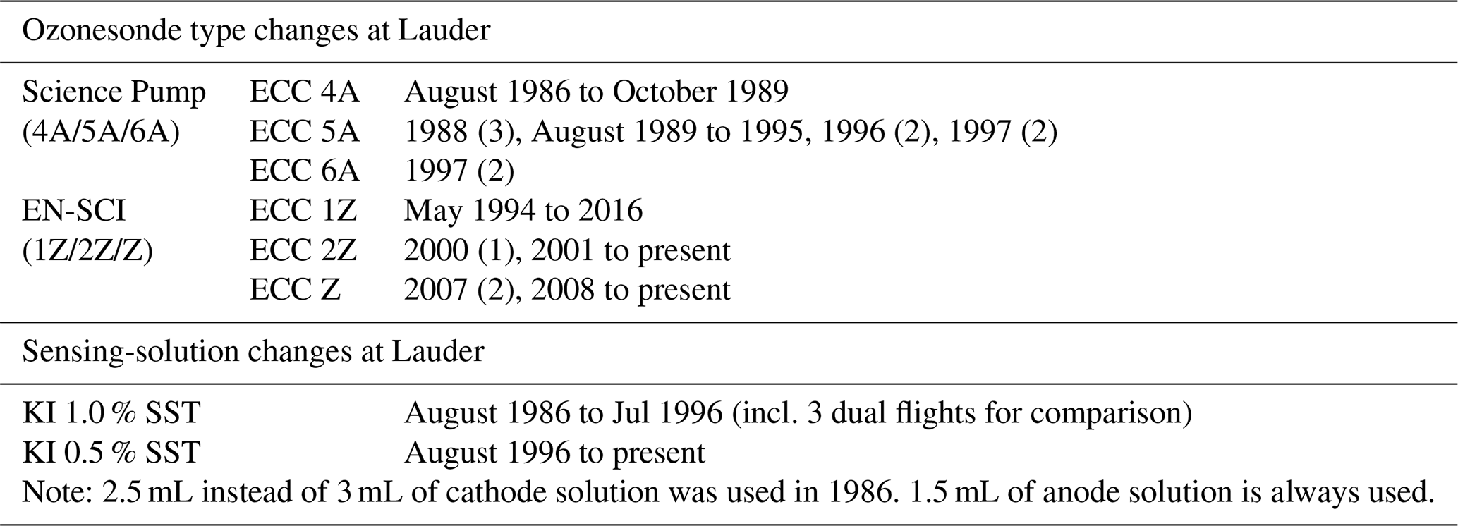
Numbers in brackets indicate the number of flights in these conditions.
The homogenisation procedure, described in the Assessment of Standard Operating Procedures for Ozonesondes (ASOPOS 2.0) documentation (Smit et al., 2021) and in the Ozonesonde Data Quality Assessment (O3S-DQA) activity (Smit and the O3S-DQA panel, 2012), was applied to the Lauder ozonesonde time series, available at NDACC. These NDACC data, named “uncorrected data” hereafter, have been obtained by converting the raw currents measured with an ozonesonde to ozone partial pressures by subtracting a measured background current using a conversion efficiency of 1.0, the measured pump temperature, and the pump flow rate measured prior to launch in the lab and then correcting for the pump efficiency decrease with increasing altitudes. The O3S-DQA homogenisation, however, adds corrections to the pump temperature, the pump flow rate (due to the moistening effect), and the background current (avoiding too-high values) on top and uses a set of transfer functions applied to the conversion efficiency to remove biases due to changes in the instrument or operating procedures. For instance, as the 0.5 % KI solution has become the recommendation for the EN-SCI ECCs, a transfer function is applied to the profiles between 1994 and 1996, where the 1 % KI solution instead of the 0.5 % KI solution was used for the EN-SCI ECCs at Lauder. The re-processing of the Lauder data according to the O3S-DQA guidelines was carried out by the HEGIFTOM working group (Harmonization and Evaluation of Ground Based Instruments for Free Tropospheric Ozone Measurements, https://hegiftom.meteo.be, last access: 21 May 2024) within the TOAR-II (Tropospheric Ozone Assessment Report phase II, https://igacproject.org/activities/TOAR/TOAR-II, last access: 21 May 2024) initiative. Further details regarding the corrections are summarised in Appendix A.
In this study, we include a total of 1958 ozonesonde flights between August 1986 and June 2021, the data of which have been homogenised. Both homogenised and measured uncorrected datasets have been post-processed for linear trend calculations. The homogenised data are used in the MLR analysis. Linear piecewise regression was applied to interpolate the original ozone profiles from the surface to 30 km at a 1 km vertical resolution. We then exclude some extreme ozone values, identified as the values that are outside the 3-standard-deviation range, to create monthly means by averaging the data available for that month at each re-gridded vertical level.
2.2 Multiple linear regression model
We construct a multiple linear regression (MLR) model to identify the dominant factors that are associated with O3 variations and trends. The regression model approximates the annual mean ozone anomalies for each level, as well as for eight grouped layers where annual mean ozone anomalies are averaged (0–1.5, 1.5–3, 3–6, 6–9, 9–12, 12–15, 15–20, and 20–25 km). The auto-correlations that usually exist in the monthly varying data have been largely removed by averaging them into annually varying data. The purpose of this study is to analyse the interannual variations and trends in annual mean ozone. The regression models include nine terms representing the solar index (SI), which captures solar variability and is defined by the solar radio flux at 10.7 cm, the multivariate El Niño Southern Oscillation Index (MEI), the quasi-biennial oscillation at 30 and 10 hPa (QBO30 and QBO10, respectively), the tropopause height (HTTrop), the stratospheric temperature (TStrat), the surface relative humidity (RHsurf), the aerosol optical depth (AOD), and the equivalent effective stratospheric chlorine (EESC). The two QBO indices are orthogonalised with respect to each other. The EESC is defined as a relative measure of the potential for stratospheric ozone depletion that combines the contributions of chlorine and bromine from surface observations from ODSs (Newman et al., 2007) and is calculated based on the ozone-depleting substances from the Coupled Model Project 6 (CMIP6) historical (until 2014) and Shared Socio-economic Pathway (SSP245) (for 2015–2021) scenarios (Meinshausen et al., 2017). Surface relative humidity is measured by the radiosonde that has a humidity sensor. We define the tropopause based on the WMO lapse rate definition (World Meteorological Organization, 1957), which is calculated from the temperature measured by the radiosonde during each ozonesonde flight. The regressed O3 anomaly is expressed as
Here, Ozone(t) is the annual mean ozone anomaly; ϵ is the regression residual, minimised in the rms; and a1−9 are the regression coefficients for the corresponding regressors, all normalised to vanishing means and unit standard deviation (i.e. standardised). All forcings used in the regression are summarised in Table 2.
(World Meteorological Organization, 2011)NASA/LARC/SD/ASDC (2022)(World Meteorological Organization, 1957)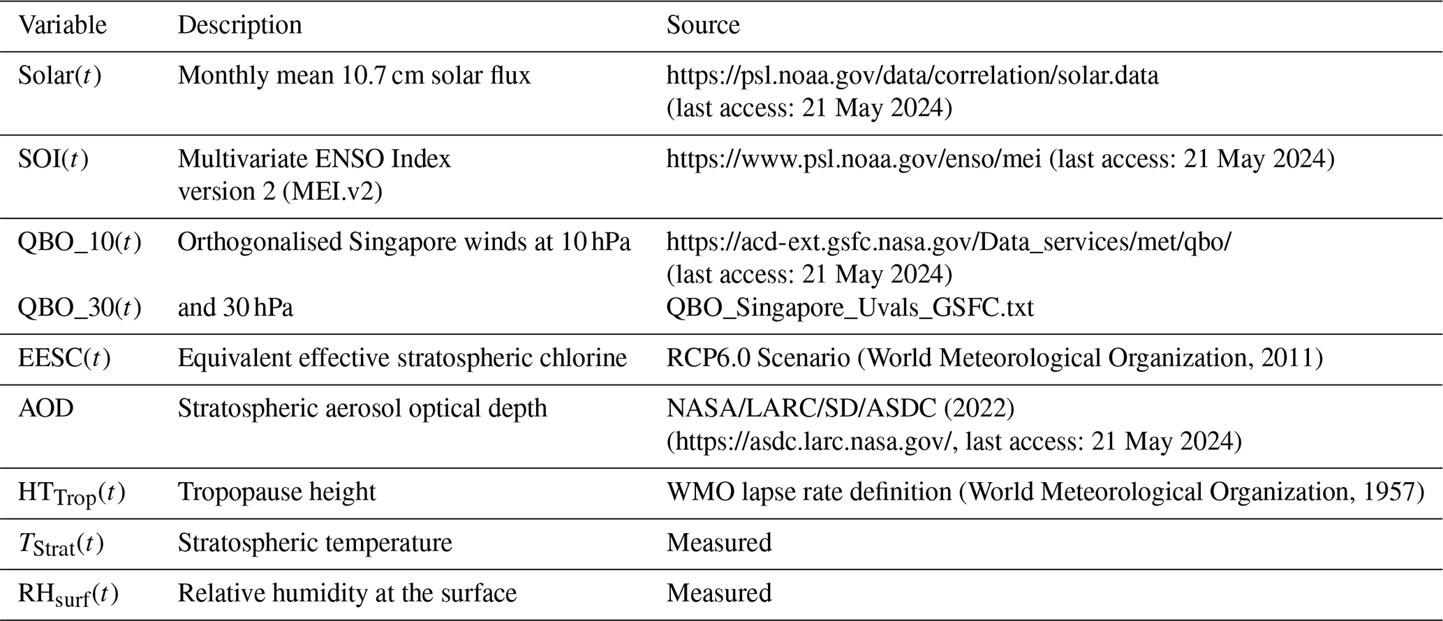
2.3 Chemistry–climate model simulations
We use the NIWA-UKCA model simulations from the Chemistry-Climate Model Initiative project (CCMI-1: Eyring et al., 2013; Morgenstern et al., 2017) to assess the impact of the major anthropogenic forcings, including greenhouse gases (GHGs) and ozone-depleting substances (ODSs), on ozone changes at Lauder. The Lauder ozonesonde measurements cover both the ozone depletion and the recovery periods of 1987–2020. Global chemistry–climate models (CCMs), including NIWA-UKCA (Morgenstern et al., 2009; Zeng et al., 2015, 2017), generally have coarse spatial resolutions. Therefore, it is often not ideal to use the simulations from the CCMs for reproducing the observed trends at a specific location. Instead, the CCMs can be used to attribute the trends to various forcings on a wider spatial and temporal scale. Here, we calculate the ozone trends using the NIWA-UKCA simulations to gauge the impacts of GHGs and ODSs on ozone changes at Lauder over the observational period in a limited area (averaged over 40–50° S and 160–180° E). We also show the simulation results on a global scale in context. The CCMI-1 simulations from NIWA-UKCA used here consist of all the forcings (including time-varying GHGs, ODSs, and ozone and aerosol precursors) of the coupled atmosphere–ocean reference experiment “RefC2”, covering the simulation period of 1960–2100 (we keep the same experiment naming convention as defined by Eyring et al., 2013) and its corresponding fixed single-forcing sensitivity experiments (sen-C2-fODS, sen-C2-fGHGs, sen-C2-fCH4, and sen-C2-fN2O) in which ODSs, the combined GHGs, methane (CH4), and N2O are individually fixed at their 1960s levels. The impact of each single forcing on ozone is derived from the differences in ozone between the RefC2 ensemble mean (five members) and the ensemble averages of the corresponding fixed single-forcing simulations (one to three ensemble numbers for each experiment). We directly assess the impacts of changes in ODSs, combined GHGs, methane, and N2O on ozone trends based on available simulations. However, no simulation was performed to directly assess the impact of CO2 within CCMI-1; instead, it will be assessed by subtracting the impacts of methane and N2O from the impact of the combined GHGs (Morgenstern et al., 2018). We again separately examine the changes in modelled ozone trends over the periods of 1987–1999 and 2000–2020. The detailed description of the model and experiments can be found in Morgenstern et al. (2018) and in Zeng et al. (2017) and the references therein.
3.1 Homogenised versus uncorrected ozonesonde time series
The homogenised and the uncorrected datasets are directly compared without any temporal interpolation but are both interpolated to a 1 km vertical grid using piecewise linear regression. Figure 1 shows the percentage difference between vertical ozone profiles from the two datasets for all flights. The correction procedure and the impact of each correction are described in more detail in Appendix A. Overall, corrections lead to mostly increased ozone values in the homogenised time series, reaching 6 % to over 10 % before 1995 due to the pump temperature correction (Fig. A1c in the Appendix). The pump flow rate correction results in a uniformly positive effect of less than 2 % in general (Fig. A1d). There are scattered increases in ozone in the homogenised time series compared to the uncorrected data, especially between 2012 and 2015, when a modified background current correction is applied (Fig. A1b). The effect of the changes in the KI solution concentration on the conversion efficiency (Fig. A1a) is mainly negative between 1994 and 1996 but positive in the beginning of the time series (1986), when a smaller cathode sensing solution amount was used (2.5 mL instead of 3 mL).
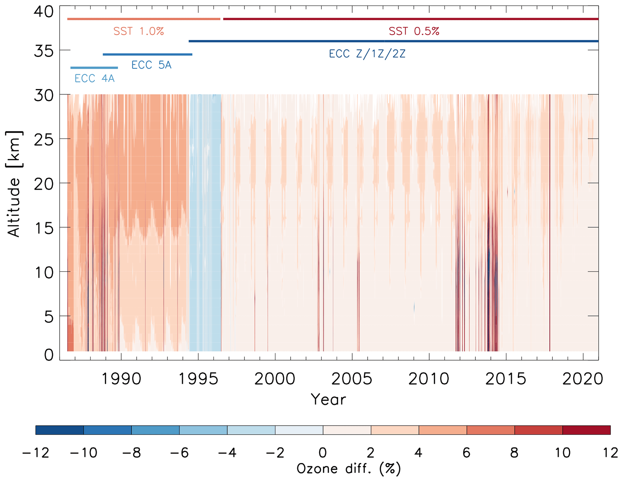
Figure 1Comparison of ozonesonde time series before and after homogenisation over 1987–2020 for all flights in terms of percentage difference between homogenised data and uncorrected data (i.e. ). Also shown are periods indicating changes in the ozonesonde type and the solution used.
The differences between the homogenised and the uncorrected monthly mean ozone time series are calculated, excluding outliers defined for ozone outside the 3-standard-deviation interval of all data points for that level (Fig. 2). This step removes fewer than 1 % of data points from the monthly mean ozone calculations. Most of these outliers are around 10 km, where the ozone is subjected to large dynamical variations.
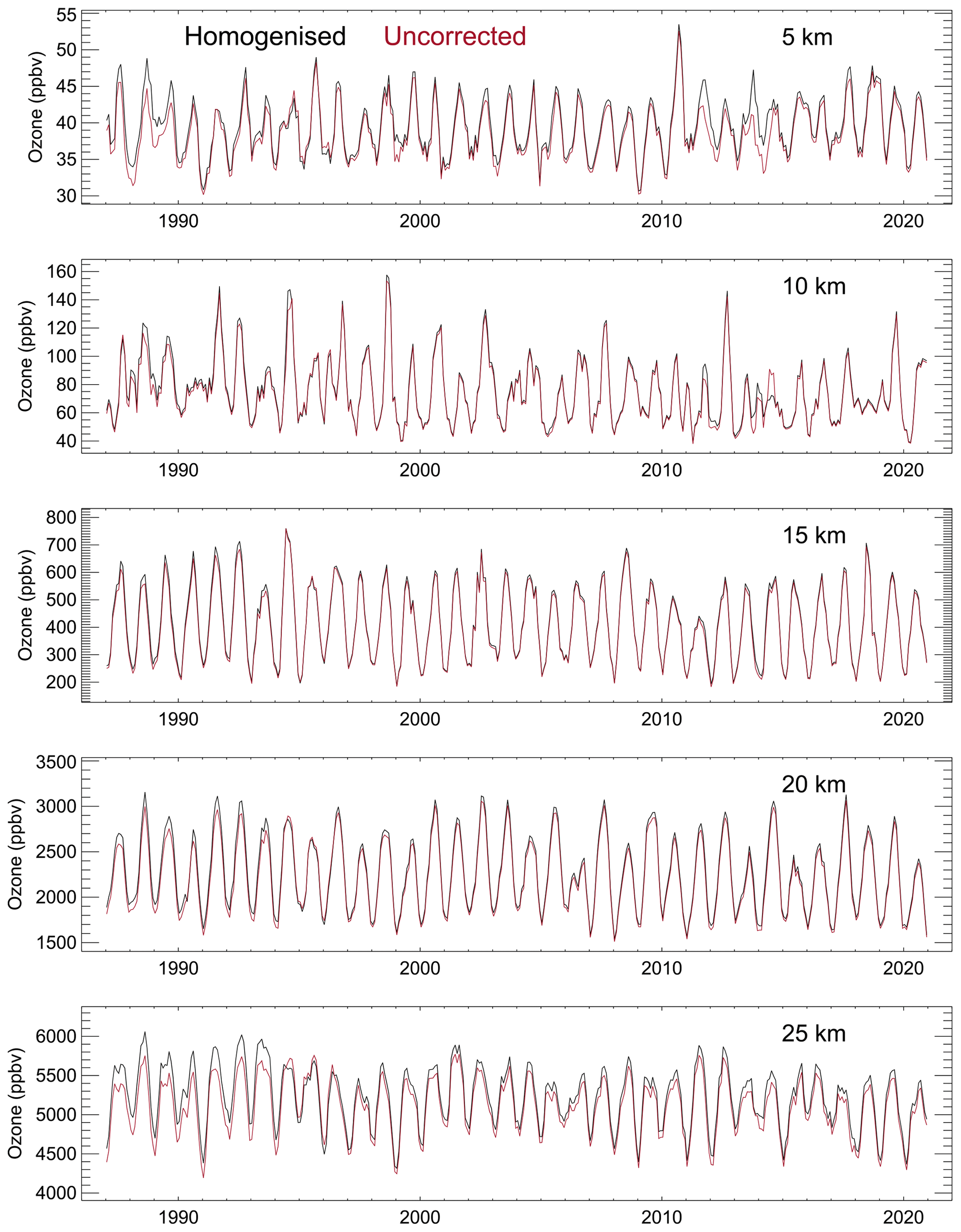
Figure 2The homogenised and the uncorrected monthly mean ozone values (ppbv) for different vertical layers over 1987–2020. For display purposes, the monthly data are smoothed with a 3-month boxcar filter.
3.2 Vertically resolved trends in observed ozone at Lauder
Consequently, the trend in ozone can be affected by the homogenisation. Here, we calculate simple linear trends in the two datasets for comparison. Figure 3 displays linear trends from the surface to 30 km for both homogenised and uncorrected datasets over the pre-1999 and post-2000 periods, respectively. Also displayed is the observed FTIR ozone trend for the post-2000 period for comparison. All trend calculations use annual mean ozone anomalies to minimise the auto-correlation in data as opposed to using the monthly mean data. This shows that there are systematic differences in ozone trends in the homogenised data compared to in the uncorrected data over the 1987–1999 period (Fig. 3a). During this period, the vertically resolved trends in the uncorrected dataset are slightly negative throughout most of the domain above 10 km and positive below 10 km, although these trends are generally insignificant at the 95 % confidence level. In contrast, the trends in the homogenised data are negative throughout the domain (∼ −2 % per decade to −13 % per decade), with most of the trends below 5 km and above ∼ 24 km being statistically significant at the 95 % confidence level. This result is more consistent with the impact of increasing ozone-depleting substances (ODSs) over this period.
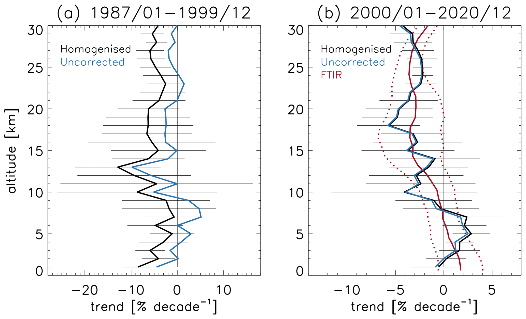
Figure 3Vertically resolved observed linear trends in monthly mean ozone and their uncertainties (± 2σ) at Lauder over two periods, i.e. 1987–1999 (a) and 2000–2020 (b), from ozonesonde measurements (black: homogenised data; blue: uncorrected data) and from FTIR measurements (red for the 2001–2021 period). Note the slightly different time period for the FTIR ozone data.
In the post-2000 period, the calculated trends are very similar between homogenised and uncorrected ozone profiles (Fig. 3b). Both show significant positive trends of up to ∼ +2 % per decade in the free troposphere and a significant negative trend of ∼ −2 % per decade to −6 % per decade above ∼ 16 km in the stratosphere, which peaks around 18 km. We note that the lower-stratospheric ozone negative trend of ∼ −3 % per decade to −6 % per decade between 15 and 20 km looks visibly smaller in magnitude than the trend presented in Godin-Beekmann et al. (2022), where it exceeds −6 % per decade in the same region, but both of these are within the uncertainty ranges displayed by Godin-Beekmann et al. (2022). Distinct negative trends of ∼ 2 % per decade to 4 % per decade also exist in the upper troposphere and the lower stratosphere between 8 and 16 km, albeit with large statistical uncertainty, highlighting the large dynamical variability typical for this region. We find that the vertically resolved ozone trends calculated by excluding the outliers are very similar to the trends calculated by including all data points. The only difference is that, by excluding the outliers, we have reduced the trend uncertainties around the 10 km region (not shown). The vertically resolved trends in observed ozone for the post-2000 period are in excellent agreement with the trends derived from the FTIR ozone data (Fig. 3b). Note that the updated FTIR ozone data presented here, obtained using an updated retrieval strategy (García et al., 2022; Björklund et al., 2023), are markedly different from the FTIR data shown by Godin-Beekmann et al. (2022). The negative trends in the lower stratosphere in both the sonde and the FTIR ozone data shown here are noticeably larger in magnitude than the trends in the satellite data shown by Godin-Beekmann et al. (2022), which have typically insignificant trends of less than −2 % per decade.
3.3 Variations and trends explained by the MLR analysis
The regression model (Eq. 1) was constructed using annual mean ozone anomalies of the homogenised ozonesonde data (hereafter, we refer to the homogenised ozone dataset as the “observed” ozone at Lauder). The regression is performed for each level from the surface to 30 km at a 1 km resolution, and the linear trend of the predicted ozone at each level was then calculated. Figure 4 shows that the vertically resolved ozone trends from the MLR-predicted ozone are quite similar to the simple linear trends in the observed ozonesonde data, but the uncertainties in the MLR-predicted ozone trends are generally smaller than those in the observed trend. The trends in the MLR-predicted ozone are also systematically smaller in magnitude in the stratosphere above ∼ 18 km for both periods, but the difference is slightly larger for the post-2000 period, though both are within the uncertainty ranges of the observed trends. This indicates that the regressors used in the MLR model do not fully capture the observed trend there. Despite the slight differences in magnitude, trends calculated here and by Godin-Beekmann et al. (2022) point to the fact that significant negative trends in the lower stratosphere exist in Lauder ozonesonde data, and these negative trends are underestimated by the satellite products.
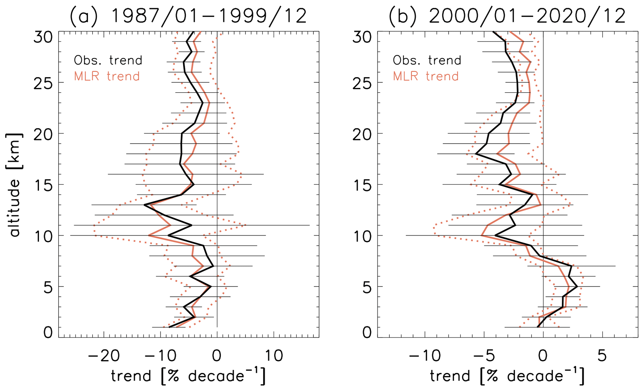
Figure 4Vertically resolved linear trends in regressed ozone (orange) and in the homogenised observed ozone (black) and their uncertainties (± 2σ) at Lauder over two periods, i.e. 1987–1999 (a) and 2000–2020 (b). Data used for linear trend calculations in both cases are annual mean anomalies.
We then group the vertical ozone profile into eight layers from the surface to 25 km in order to identify the drivers of ozone variability and trends for each vertical layer. The same MLR is performed individually for each layer. The observed and regressed ozone anomalies, together with the leading contributions from individual regressors, are shown in Fig. 5. The ozone variance explained by the regression is given by the multiple regression coefficient of determination R2 (Fig. 5 and Table 3). The standardised individual regression coefficients for each regressor can be used to measure their contributions to the total variance explained at that level (Table 3).
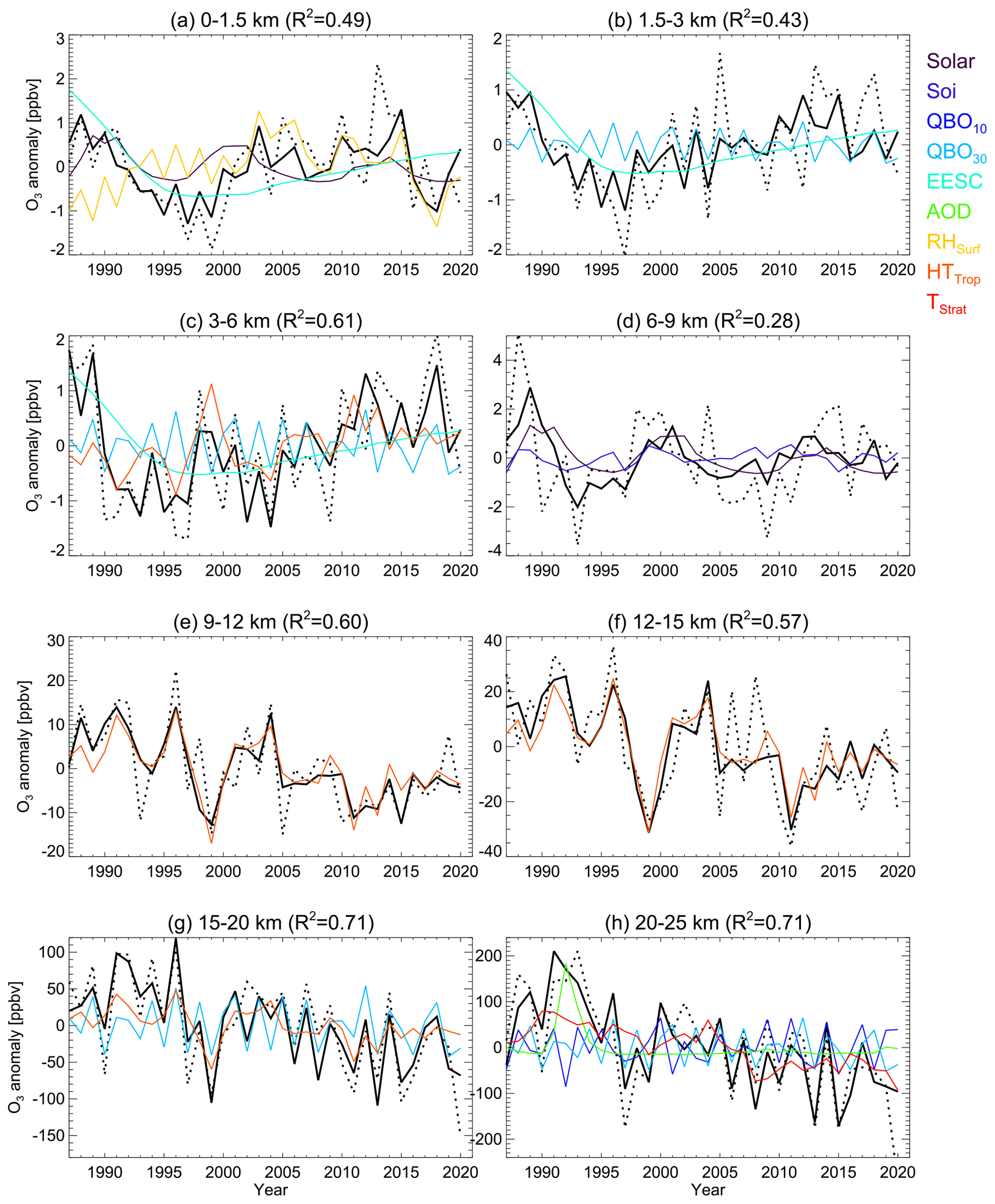
Figure 5Regressed ozone anomalies (black curves) and observed ozone anomalies (dotted black curves, homogenised data) at Lauder (1987–2021) for eight vertically averaged layers. Contributions from leading regressors for each layer are displayed in coloured curves (colour key is to the right of the plots).
Table 3Coefficient of determination R2 for each altitude band (km) and the standardised regression coefficients ± 2σ (standard error). The regression coefficients in bold are statistically significant at the 95 % confidence level.
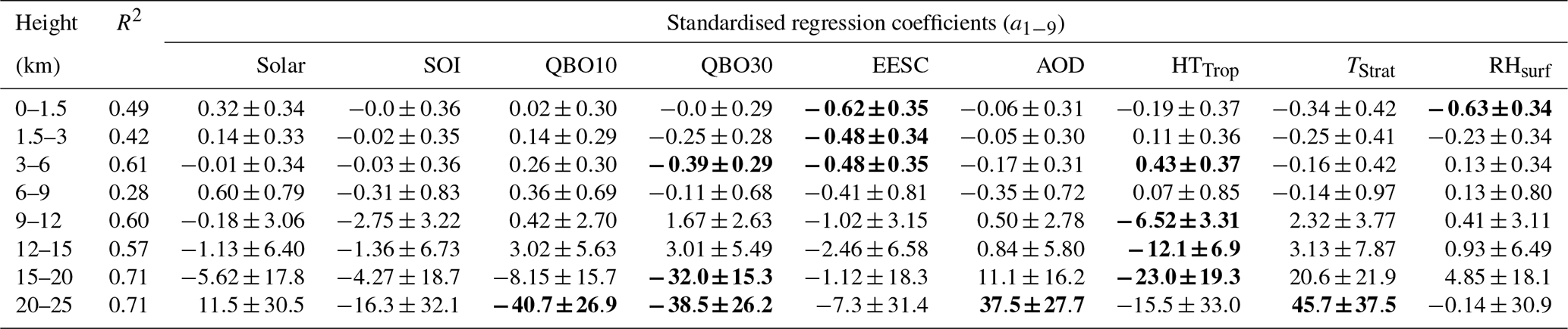
The regression model matches the observed anomalies well, particularly in the stratosphere, the upper troposphere, and near the surface (Fig. 5 and Table 3). With R2 values ranging from 0.28 to 0.61 in the troposphere and 0.57 to 0.71 in the stratosphere, the stratospheric ozone variations and trends are better captured by the MLR model than tropospheric features. Indeed, interannual variations in ozone anomalies in the upper troposphere and the lower stratosphere (9–15 km) are especially well explained by variations in tropopause height (Fig. 5 and Table 3). The downward trend in the stratospheric ozone between 9 and 20 km is clearly driven by the significant positive linear trend in tropopause height (Fig. 6c). The QBO at 30 hPa, together with tropopause height, also explains a large part of the ozone variability for the 15–20 km layer (Fig. 5 and Table 3). Above 20 km, the QBO at both 30 and 10 hPa, the AOD, and the stratospheric temperature (TStrat) have a significantly negative trend (Fig. 6b). We note that the correlation between AOD and the Lauder stratospheric ozone is positive, e.g. after the Mt Pinatubo eruption in 1991, despite the potential ozone depletion in the years following a volcanic eruption (Fig. 5h). This lack of ozone depletion was attributed to the perturbation of the stratospheric dynamics by the Mt Pinatubo eruption that obscured the chemical effect in the southern extra-tropics (Aquila et al., 2013). We also note that the prolonged decline in ozone above 15 km at the end of the time series (around 2020) cannot be explained by the MLR model (Fig. 5g and h); this might be the result of the Australian bush fires in January 2020, which depleted stratospheric ozone (Salawitch and McBride, 2022). The lack of this process in MLR might also explain the weaker negative trend in the regressed ozone compared to that in the observed ozone above 18 km (Fig. 4b).
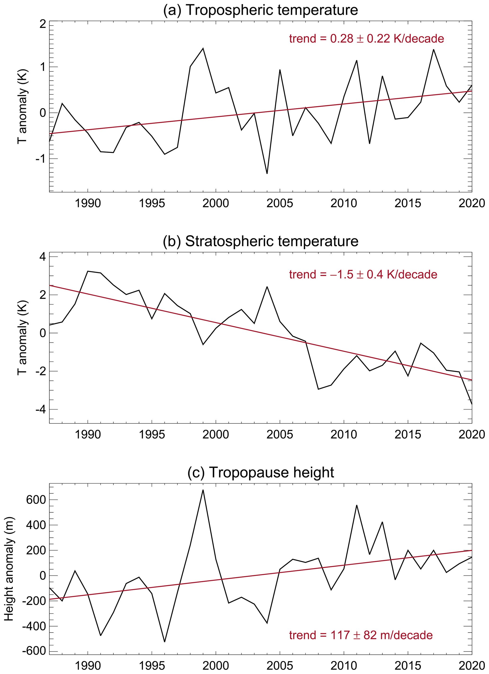
Figure 6Annual mean anomalies of observed tropospheric temperature (averaged below 5 km) (a), stratospheric temperature (averaged between 22 and 30 km) (b), and the tropopause height (c) and their linear trends (± 2σ) at Lauder.
It is well established that increases in CO2 influence temperature, humidity, and circulation, which in turn affect ozone chemistry and transport (Brasseur and Hitchman, 1988; Butchart et al., 2006; Fleming et al., 2011). Warming in the troposphere and cooling in the stratosphere due to the increase in CO2 have driven the increase in tropopause height over the last several decades based on radiosonde observations, reanalysis data, and modelling (Highwood et al., 2000; Seidel et al., 2001; Seidel and Randel, 2006; Santer et al., 2003a, b; Meng et al., 2021). The tropopause height derived from the Lauder sonde data shows a significant positive trend of 117 ± 82 m per decade (at 95 % confidence) over the observational period, calculated as the simple liner trend in the annual mean anomaly (Fig. 6c), which is larger than the trend of ∼ 50–60 m per decade in the Northern Hemisphere (20–80° N) over 2001–2020 based on radiosonde data (Meng et al., 2021).
However, in the middle and upper troposphere (6–9 km), the regression function explains less of the ozone variation compared to at levels above and below (Fig. 5d). Here, although the solar influence is the strongest in relative terms, influences from all other regressors, except the QBO at 10 hPa, contribute non-negligibly to explaining the ozone variations at this level.
In the lower and free troposphere (below 6 km), the sharp decreases in ozone during the early period of the record and the large negative anomalies in 1997–1998 are well reproduced by the regression, along with the subsequent increases in ozone there. This trend transition in tropospheric ozone coincides with the evolution of EESCs, which increased from the late 1980s before declining after 1997; this indicates that the impact of stratospheric ozone changes due to changes in ODSs could impact tropospheric ozone through transport. Indeed, the interannual variation in the free tropospheric ozone is shown to be influenced by the QBO at 30 hPa (Fig. 5b and c). In the troposphere, increases in ODSs are expected to drive an increase in ozone after the late 1990s, whilst the response to the CO2 increase is more complex. For instance, the associated increasing humidity would lead to more chemical destruction of ozone in the troposphere, and the increase in temperature may result in more ozone production through NOx–CH4 (and volatile organic compound) chemistry (e.g. Stevenson et al., 2006; Zeng et al., 2008). Here, relative humidity and surface ozone are anti-correlated (Fig. 5a). Relative humidity has a large negative impact on surface ozone (Table 3). Moreover, we have not considered changes in ozone precursor concentrations and other meteorological parameters in the regression that could substantially impact tropospheric ozone. Therefore, more explanatory variables can be included in an MLR model that is specifically focused on tropospheric ozone; this is the subject of a future study.
3.4 Attribution of modelled Lauder ozone changes to ODSs and GHGs
We examine the modelled vertically resolved ozone trends in the vicinity of Lauder (40–50° S and 160–180° E) from the NIWA-UKCA model over the ozone depletion (1987–1999) and recovery (2000–2020) periods separately, along with the effects of changes in ozone trends due to individual forcings, using the same approach as in Zeng et al. (2022). Meanwhile, in order to help understand Lauder ozone changes in a global context, we also show the modelled zonal mean ozone trends covering all latitude bands and the changes that are attributable to ODSs and GHGs (Appendix B). The modelled and attributable trends are linear trends in diagnosed annual mean ozone anomalies calculated from model simulations.
3.4.1 Pre-1999 period
Over the ozone depletion (pre-1999) period, the modelled ozone trends at Lauder (Fig. 7a) are significantly negative (at the 95 % confidence level) throughout the height range covered by the sondes, and the magnitude maximises at ∼ −5 % per decade at around ∼ 14 km. The modelled trends over this period are qualitatively in agreement with the Lauder observations, although the observed trends in magnitude are generally underestimated, especially in the lower stratosphere (∼ 10–13 km), where the observed negative ozone trend is much larger at ∼ −12 % (Figs. 4a and 7c).
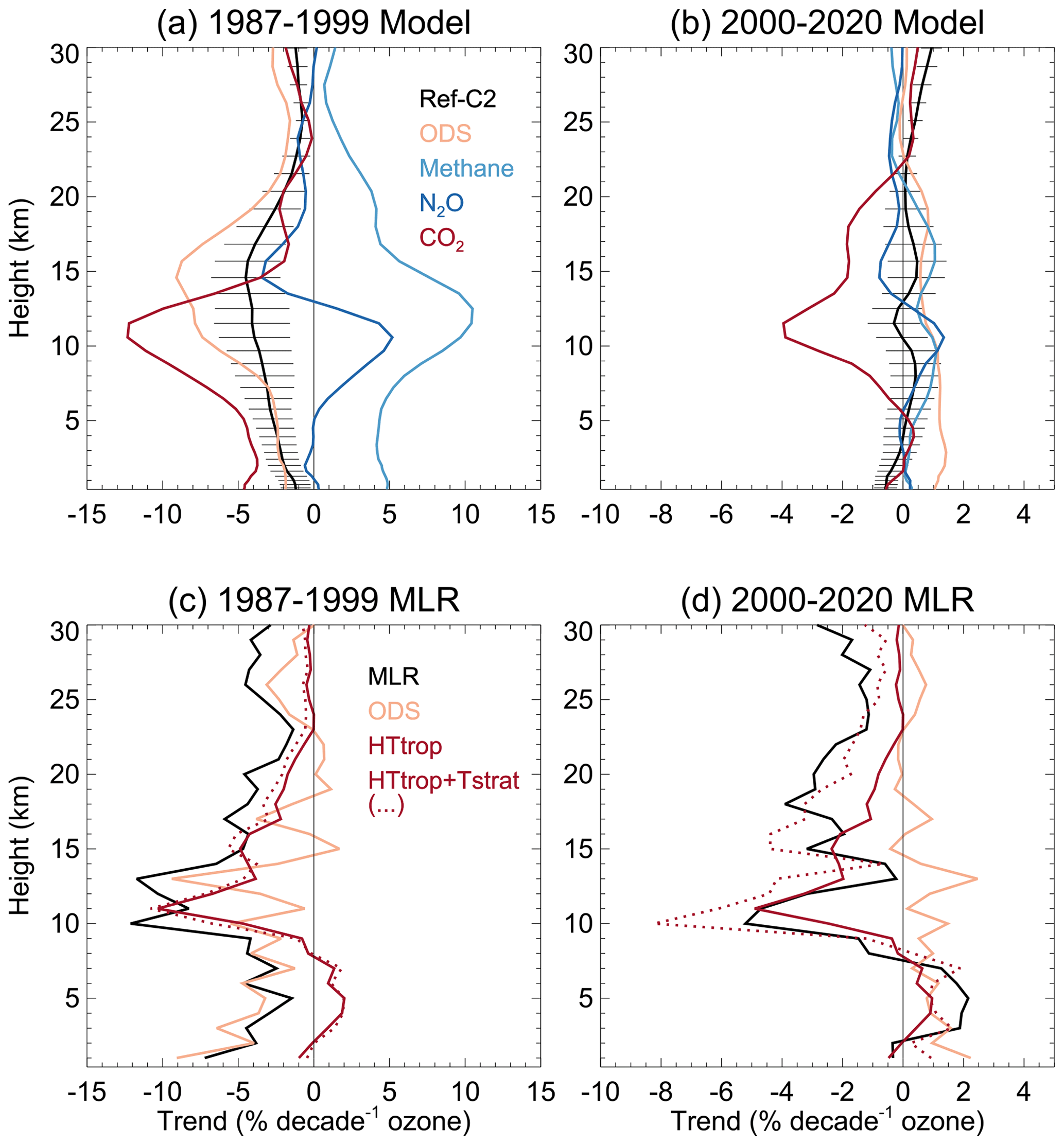
Figure 7(a, b) Vertically resolved trends in modelled annual mean ozone anomalies averaged over the area of 40–50° S and 160–180° E (representing the location of Lauder) for the periods of 1987–1999 (a) and 2000–2020 (b) from the NIWA-UKCA CCMI RefC2 simulation with the 2σ uncertainty range and the trend changes due to changes in the ozone-depleting substances (ODSs), methane, nitrous oxide (N2O), and CO2 over the same period. (c, d) Vertically resolved ozone trends in the predicted ozone (at 1 km resolution) by the multiple linear regression (MLR) and the contribution from EESC (i.e. ODSs), the tropopause height, and the combination of the tropopause height and the stratospheric temperature changes (dotted line) for the periods 1987–1999 (c) and 2000–2020 (d).
The modelled Lauder ozone trends over this period are attributable to increases in ODSs, methane, N2O, and CO2 (Fig. 7a); the uncertainties of these contributions are displayed separately in Fig. B1. The increase in ODSs contributes significantly to the negative ozone trend in the lower stratosphere (∼ 9–18 km), which is the result of ozone depletion at SH mid-latitudes (Fig. B2c). The increase in methane during this period (1987–1999) has a considerable positive impact on ozone trend over Lauder, which maximises at around 12 km (Fig. 7a) and is statistically significant at the 95 % confidence level below 15 km (Fig. B1b). The ozone increase caused by the growth of methane is partly due to its reaction with chlorine, which leads to reduced ozone depletion, especially in the stratospheric polar region, and partly due to chemical ozone production in the troposphere (Fig. B2d). The N2O increase also contributes moderately to the negative ozone trends above ∼ 13 km over Lauder, but the effect is not statistically significant at 95 % confidence (Figs. 7a and B1c). In contrast, the N2O increase leads to ozone increase in the upper troposphere (5–13 km) as a result of the self-healing effect which was explained by Morgenstern et al. (2018). The increasing CO2 (derived from the all-GHG forcing and the separate methane and N2O forcing experiments) has a relatively large negative contribution to ozone over Lauder below 20 km, which maximises at a lower altitude of around 10–12 km and is statistically significant at the 95 % confidence level below 13 km (Figs. 7a and B1d). This shows that the impacts of dynamical changes and the ozone depletion on stratospheric ozone occur at different altitudes.
We examine the contributions of ODSs and CO2-driven dynamical changes to ozone changes from the MLR model and compare those to the modelled attribution. The CO2-driven tropopause increase (Fig. 7c) exhibits a large contribution to the MLR ozone trend between ∼ 9 and 22 km, maximising at ∼ 10–12 km, which is consistent with the model attribution (Fig. 7a). The stratospheric cooling shows a small negative impact (reflected in TStrat) on the MLR ozone trend over this period. The contribution of ODSs to the regressed negative ozone is most pronounced above 23 km and below ∼ 17 km, which is again consistent with the modelled attribution. However, the impact of ODSs on the stratospheric ozone trend shown here is not reflected in the small and insignificant regression coefficient due to EESC in the stratosphere (Table 3); most likely, the impact of EESC is obscured by the more prominent impact of CO2-driven dynamical changes throughout the whole observational period and not just for the pre-1999 period. The post-2000 period would see the impact of EESC dropping considerably, explaining the small regression coefficient. We also see that the tropospheric ozone trend in the MLR model is mostly attributable to ODS changes (Fig. 7c), likely the result of stratospheric polar ozone changes through transport (Fig. B2c).
3.4.2 Post-2000 period
The stratospheric equivalent chlorine reached its maximum in the late 1990s and has been declining since. Consequently, over the period of 2000–2020, the model shows a small but largely significant positive ozone trend of up to 1 % per decade above ∼ 23 km in the stratosphere (Fig. 7b). There is no significant trend in modelled ozone below 23 km, except for a small negative trend near the surface. Clearly, the model cannot reproduce the significant negative trend in the lower stratosphere exhibited by observed ozone and underestimates observed trends at all levels in this period (Figs. 4b and 7d). In a recent assessment, combined satellite datasets indicate a negative trend over the period of 2000–2020 in the SH mid-latitude (35–60° S) of the lower stratosphere, but multi-model results generally show non-significant positive trends (Godin-Beekmann et al., 2022; World Meteorological Organization, 2022), which is typically associated with a large dynamical variability in this region.
Over this period, the effects of ODSs, methane, and N2O on modelled ozone are generally small (Fig. 7b) and statistically insignificant at the 95 % confidence level (Fig. B1). The impact of ODSs is consistently positive from the surface to about 23 km as a result of ODSs declining. The impact from methane is a small positive contribution to the modelled ozone trends, whilst the N2O mainly contributes negatively above ∼ 13 km and positively below (Fig. 7b). In contrast, the impact of CO2 on ozone at Lauder is negative between ∼ 5–22 km and maximises at ∼ 12 km, with a contribution of −4 % per decade (Fig. 7b). Although the impacts of the CO2 increase are much larger than those from other forcings during this period, the trend is not statistically significant (Fig. B1h), possibly due to the typically large dynamical variation in the UTLS region. However, on a global scale, the impact of ODSs and CO2 on ozone trends in the UTLS region can be significant at the SH mid-latitudes (Fig. B3). Here, the modelled results are consistent with previous findings on the response of global ozone changes to ODSs and GHGs using either the CCMI-1 (Morgenstern et al., 2018) or Aerosol and Chemistry Model Intercomparison Project (AerChemMIP) simulations (Zeng et al., 2022).
The attribution of MLR ozone trends shows that the impact of CO2, reflected in the change in tropopause height, is an important driver for the observed negative ozone trends at Lauder in the UTLS region after 2000, while the ODSs have been declining (Fig. 7d). This also shows that continuous stratospheric cooling, driven by the CO2 increase, plays an increasingly important role in contributing to the negative stratospheric ozone trend above 15 km observed at Lauder since 2000 (Fig. 7d). The role of ODSs during this period is consistent with the modelled attribution, which is largely positive but small.
We have updated the Lauder ozonesonde time series by homogenising the dataset with a series of well-defined correction steps accounting for changes in hardware and operating procedures. We have analysed this homogenised dataset for vertically resolved linear ozone trends over the 1987–1999 and 2000–2020 periods, characterised by increasing and decreasing trends in total chlorine and bromine, respectively. There are significant differences between the homogenised and the uncorrected data for the pre-1999 period due to these corrections, in which the uncorrected data are biased low compared to the homogenised data in general. This leads to significantly stronger negative stratospheric ozone trends in the homogenised data compared to in the uncorrected data over the 1987–1999 period. The homogenised data typically show negative ozone trends of ∼ −6 % per decade to −2 % per decade from the surface to 30 km, with a maximum of ∼ −13 % per decade around 13 km, which is substantially stronger than trends in uncorrected data, which are largely insignificant. For the post-2000 period, the homogenisation does not alter ozone trends significantly; both datasets show significant negative trends in the stratosphere up to ∼ −6 % per decade and small positive trends of up to +2 %–3 % per decade in the troposphere. The post-2000 trends in ozonesonde data are in excellent agreement with trends in co-located FTIR ozone profiles.
In addition, we calculated linear trends in the MLR-predicted ozone for the two periods, which show a very good agreement with the observed linear trends, except for the region above 18 km, where the MLR trend is slightly smaller in magnitude in the post-2000 period. The large negative trend in the lower stratosphere is consistent with the trend calculated by Godin-Beekmann et al. (2022) based on data from the LOTUS regression model, although the negative trend found by Godin-Beekmann et al. (2022) is insignificantly larger in magnitude. The uncertainty ranges found here comfortably fit within or close to the uncertainty ranges stated by Godin-Beekmann et al. (2022). Differences in the best-estimate trends could be down to the difference between the regression models used.
By using a multiple linear regression analysis, we have identified the dominant factors driving the Lauder vertically resolved ozone trends and variations. The regression model consists of independent regressors including solar flux, the state of ENSO, the QBO at two different pressure levels, stratospheric equivalent chlorine, and the aerosol optical depth representing volcanic influences. Additionally, we have included the tropopause height anomaly, representing the dynamical variability that drives the interannual variability in ozone; the stratospheric temperature anomalies that are averaged over 22–30 km to account for the impact of stratospheric cooling induced by the CO2 increase; and surface relative humidity that reflects the effect of humidity on near-surface ozone as regressors. We find a persistent negative stratospheric ozone trend at Lauder represented by the significant positive trend in the tropopause height and the significant negative trend in the stratospheric temperature of the regression function. The variation in tropopause height largely explains the interannual variations in upper-tropospheric and lower-stratospheric ozone. Significant trends in the tropopause height (positive), the stratospheric temperature (negative), and the tropospheric temperature (positive) measured at Lauder are consistent with the well-established impact of stratospheric circulation changes driven by CO2 increases (e.g. Mitchell et al., 1995; Butchart et al., 2006). The QBO and AOD indices explain much of the stratospheric ozone variation above 20 km, and the stratospheric temperature partially explains the significant negative trend at and above this altitude. In the troposphere, the interannual variations and trends in ozone are less well explained by the regression function in comparison with those in the stratosphere. However, surface relative humidity explains a substantial amount of surface ozone variability. The impact of ODSs on tropospheric ozone at Lauder is demonstrated by the downward and upward trends in tropospheric ozone before the late 1990s and after 2000, coinciding with the increase and decrease in ODSs, respectively.
We have also used a series of chemistry–climate model single-forcing simulations to gauge the impact of changes in GHGs – including methane; N2O; and, indirectly, CO2 – and ODSs on ozone profiles at Lauder, as well as on the zonal mean ozone profiles covering all latitude bands in a global context. For 1987–1999, simulations show significant negative ozone trends throughout the vertical domain (up to 30 km), broadly in agreement with observed ozone trends at Lauder during this period, except for in the lower stratosphere, where the modelled ozone trend is substantially smaller in magnitude than the observed negative trend. Fixed single-forcing simulations attribute the negative ozone trend to ODS-driven ozone depletion in the SH mid-latitudes and to the increase in CO2, which leads to changes in stratospheric circulation and temperature that impact ozone. However, this negative impact on ozone is offset by the positive impact of methane. N2O plays a smaller role, with both negative impacts on ozone above ∼ 13 km and positive ones below that level. Note that, although the MLR coefficient representing the impact of ODSs on stratospheric ozone is small and insignificant for the whole analysis period, the impact of ODSs on stratospheric ozone is apparent from both the modelled and MLR trend attributions over the 1987–1999 period. The impact of ODSs on tropospheric ozone appears to be affected by the polar stratospheric ozone through transport.
Over the period of 2000–2020, although the model cannot capture the observed significant negative ozone trend in the upper troposphere and lower stratosphere over Lauder, it points to a significant negative impact of the CO2 increase on ozone in this region, offset by much smaller positive impacts from the reduction in ODSs and the increases in methane and N2O. This modelled negative impact from CO2 on ozone through dynamical changes is reflected in the observed tropopause height increase at Lauder, and this impact will grow if CO2 continuously increases in the future. Therefore, long-term vertically resolved monitoring of ozone is of particular importance in understanding the impact of climate change on the ozone distribution and vice versa.
The corrections that are applied to the Lauder ozonesonde time series are detailed below. All the corrections are applied to the raw ozone currents. When these cell currents were not archived in the early period, they needed to be reconstructed from the ozone partial pressure data in the NDACC archive with the available metadata (e.g. pump flow rate, pump temperature, background current, pump efficiency correction table used). Then, correction functions are applied according to those recommended in Smit and the O3S-DQA panel (2012). The effect from each correction is shown in Fig. A1.
A1 Conversion efficiency
The stoichiometry correction was applied for the 1986 data, where 2.5 mL cathode solution was used instead of 3 mL. The EN-SCI sondes with a 1.0 % buffer solution strength over the period of 1994–1996, instead of a 0.5 % strength, were also corrected.
A2 Background current
A consistent background current correction was applied to the Lauder data. If the background current values fall above the mean value + 2 standard deviations (σ), these values are replaced by the mean value. The mean and corresponding standard deviations are calculated and applied separately in two periods (i.e. before and after 1996) as the background current values are systematically larger for the period before 1996 and smaller for the period after 1996.
A3 Pump temperature measurement
The truest pump temperature correction is applied according to Eq. (13) of the O3S-DQA guidelines (Smit and the O3S-DQA panel, 2012). SPC-4A sondes (until 1989), SPC-5A (from 1989 to 1994), and EN-SCI sondes (from 1994) were launched in the configuration where the pump temperature measurement was made inside the pump. However, the SPC-4A and SPC-5A pump temperature measurements need additional corrections (see Smit and the O3S-DQA panel, 2012).
A4 Pump flow rate (moistening effect)
Equation (15) of the O3S-DQA guidelines was applied to correct the moistening effect of the pump flow rate. There are missing metadata, including the temperature and humidity of the laboratory before February 2014. The climatological means calculated for each month are then used for these missing metadata.
A5 Pump flow efficiency
Equation (22) of the O3S-DQA guidelines (Smit and the O3S-DQA panel, 2012) was applied using the pump flow correction factors (CPFs) as a function of air pressure (Table 6 of this guideline). These are also applied to the uncorrected data as a part of the conversion from the ozone currents to ozone partial pressures. The small change in these correction factors around 1994 is due to the fact that different correction factors need to be applied for SPC and EN-SCI ozonesonde pumps.
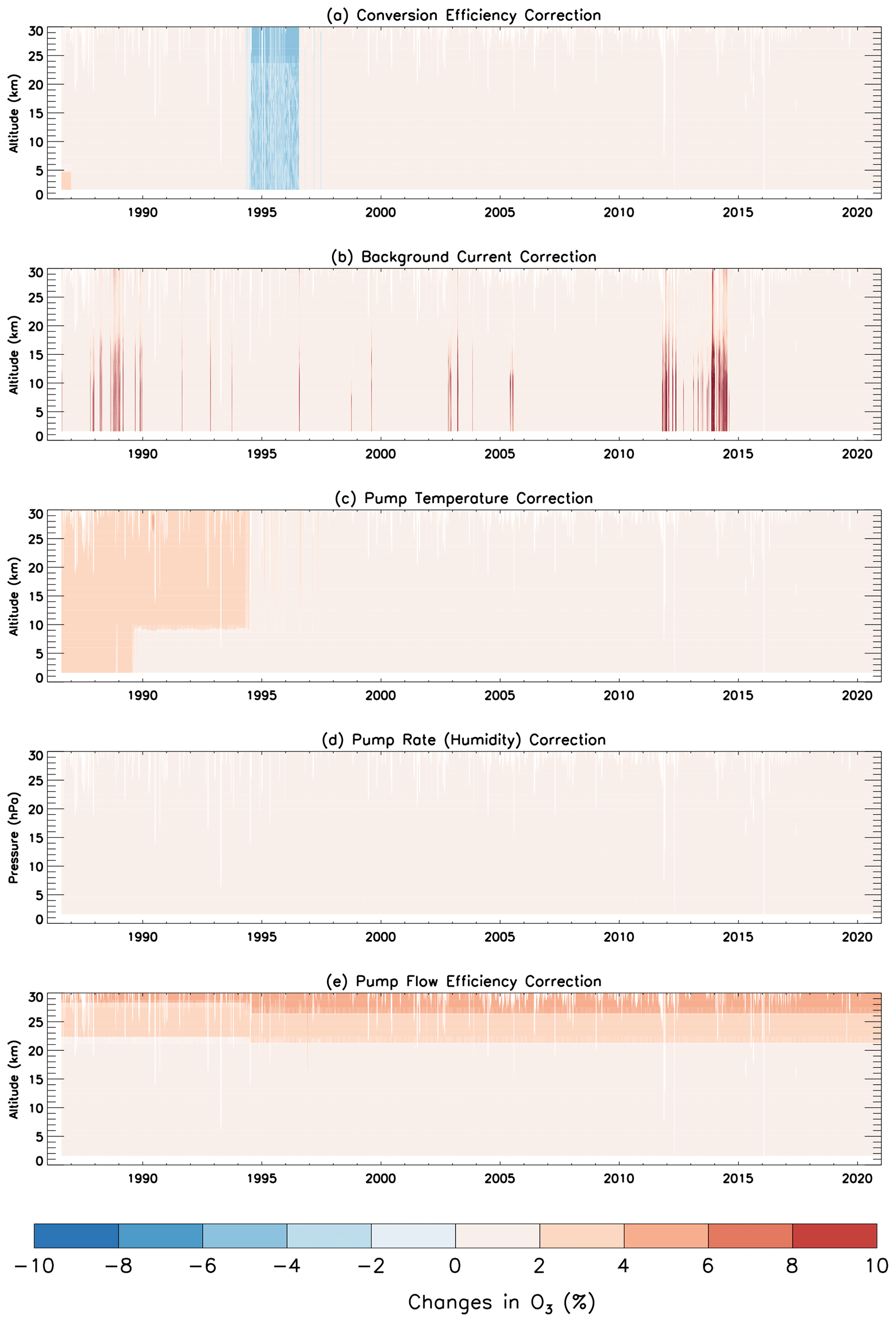
Figure A1Effect of various corrections on Lauder ozonesonde time series, expressed in percentage changes in ozone.
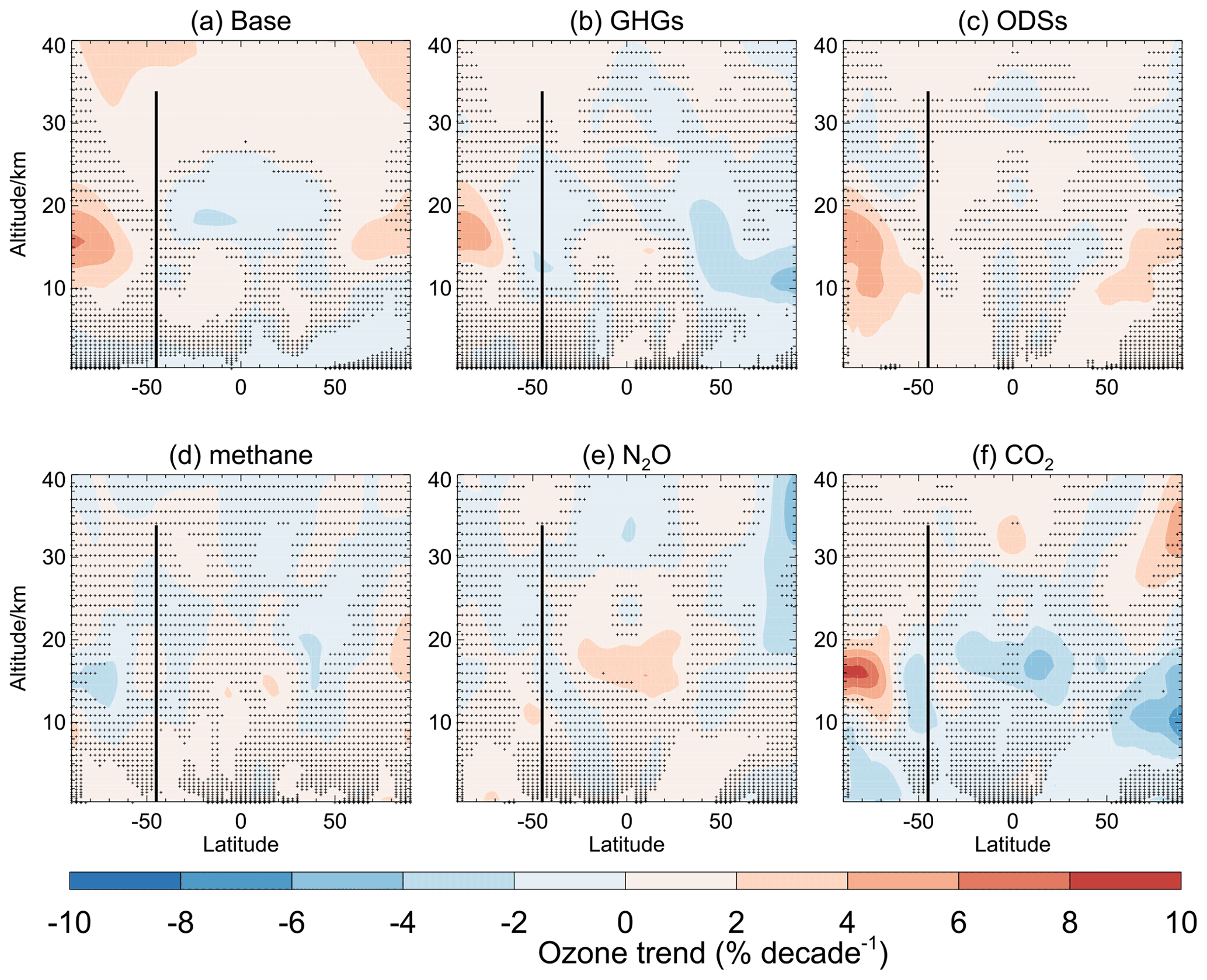
Figure B1 displays the modelled Lauder ozone trend changes due to ODSs, methane, N2O, and CO2, including the 2σ uncertainty range. Figures B2 and B3 display the modelled global zonal mean ozone trends and the impacts from ODSs, combined GHGs, methane, N2O, and derived CO2 for the periods of 1987–1999 and 2000–2020.
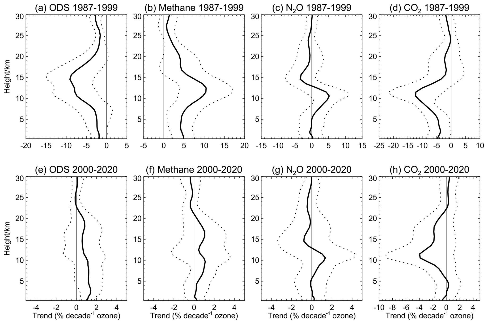
Figure B1Ozone trend changes due to changes in the ozone-depleting substances (ODSs), methane, nitrous oxide (N2O), and CO2 for the periods of 1987–1999 (a–d, respectively) and 2000–2020 (e–h, respectively) simulated in NIWA-UKCA CCMI simulations. The 2σ uncertainty range is marked by dotted lines. Trends in ozone are averaged in the area of 40–50° S and 160–180° E(representing the location of Lauder).
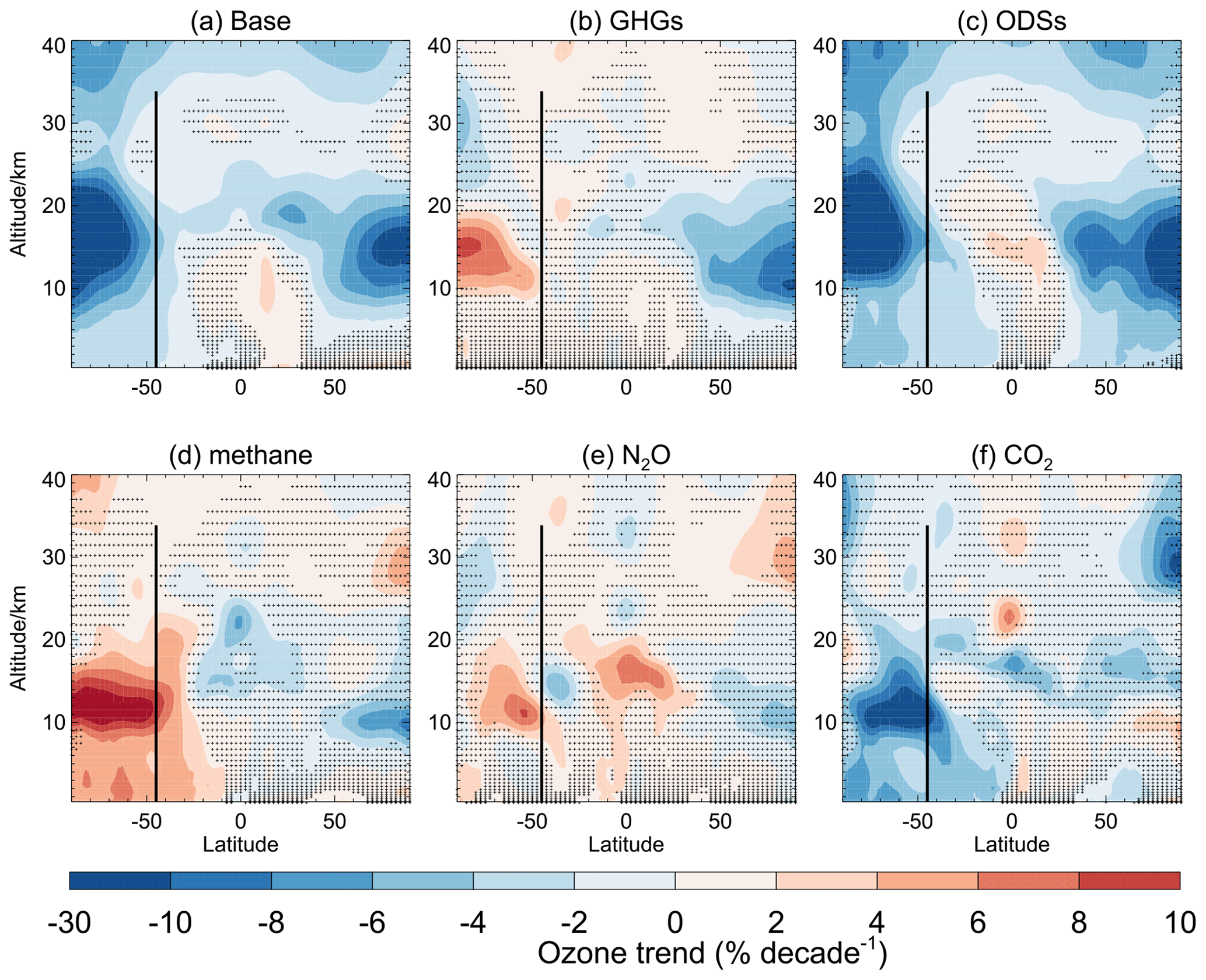
Figure B2Trends in zonal mean ozone between 1987 and 1999 from the NIWA-UKCA CCMI RefC2 simulation (a) and the change in zonal mean ozone trend due to changes in (b) greenhouse gases (GHGs), (c) ozone-depleting substances (ODSs), (d) methane, (e) nitrous oxide (N2O), and (f) CO2 over the same period. Vertical black lines indicate the latitude of Lauder Station.
The uncorrected Lauder ozonesonde data can be accessed from the World Ozone and Ultraviolet Radiation Data Centre (WOUDC) archive (https://doi.org/10.14287/10000001, WMO/GAW Ozone Monitoring Community, 2023) and from the Network for the Detection of Atmospheric Composition Change (NDACC) archive (2024, https://www-air.larc.nasa.gov/missions/ndacc/data.html). The homogenised Lauder ozonesonde data can be obtained from the TOAR-II HEGIFTOM Focus Working Group (2024, https://hegiftom.meteo.be/datasets). The CCMI-1 NIWA-UKCA ozone fields can be downloaded from the Centre for Environmental Data Analysis (CEDA) (https://catalogue.ceda.ac.uk/uuid/bf8dff222c4c4a56af7c12aa706aed0c, Morgenstern and Zeng, 2021). The instructions for access to the CEDA archive are described at https://blogs.reading.ac.uk/ccmi/ccmi-1/ (CEDA archive, 2024).
RQ, HS, AG, and PS carried out the Lauder ozonesonde measurements and processed the data. RVM and DP helped with the homogenisation of Lauder ozonesonde data. DS and JR provided the FTIR ozone time series. GZ and OM performed model simulations and conducted the statistical analysis. GZ led the writing of the paper with inputs from all the authors.
The contact author has declared that none of the authors has any competing interests.
Publisher's note: Copernicus Publications remains neutral with regard to jurisdictional claims made in the text, published maps, institutional affiliations, or any other geographical representation in this paper. While Copernicus Publications makes every effort to include appropriate place names, the final responsibility lies with the authors.
This research was supported by the New Zealand Government's Strategic Science Investment Fund (SSIF) through the NIWA programmes CACV and CAAC. We acknowledge the contribution of the New Zealand eScience Infrastructure (NeSI) High-Performance Computing Facilities to the results of this research. New Zealand's national facilities are provided by the New Zealand eScience Infrastructure and are funded jointly by NeSI's collaborator institutions and the Ministry of Business, Innovation and Employment's Research Infrastructure programme (https://www.nesi.org.nz, last access: 21 May 2024).
This research has been supported by the New Zealand Government's Strategic Science Investment Fund (SSIF).
This paper was edited by Martin Dameris and reviewed by two anonymous referees.
Ancellet, G., Godin-Beekmann, S., Smit, H. G. J., Stauffer, R. M., Van Malderen, R., Bodichon, R., and Pazmiño, A.: Homogenization of the Observatoire de Haute Provence electrochemical concentration cell (ECC) ozonesonde data record: comparison with lidar and satellite observations, Atmos. Meas. Tech., 15, 3105–3120, https://doi.org/10.5194/amt-15-3105-2022, 2022. a
Aquila, V., Oman, L. D., Stolarski, R., Douglass, A. R., and Newman, P. A.: The Response of Ozone and Nitrogen Dioxide to the Eruption of Mt. Pinatubo at Southern and Northern Midlatitudes, J. Atmos. Sci., 70, 894–900, https://doi.org/10.1175/JAS-D-12-0143.1, 2013. a
Björklund, R., Vigouroux, C., Effertz, P., Garcia, O., Geddes, A., Hannigan, J., Miyagawa, K., Kotkamp, M., Langerock, B., Nedoluha, G., Ortega, I., Petropavlovskikh, I., Poyraz, D., Querel, R., Robinson, J., Shiona, H., Smale, D., Smale, P., Van Malderen, R., and De Mazière, M.: Intercomparison of long-term ground-based measurements of tropospheric and stratospheric ozone at Lauder, New Zealand (45S), EGUsphere [preprint], https://doi.org/10.5194/egusphere-2023-2668, 2023. a, b
Bodeker, G. E., Boyd, I. S., and Matthews, W. A.: Trends and variability in vertical ozone and temperature profiles measured by ozonesondes at Lauder, New Zealand: 1986–1996, J. Geophys. Res.-Atmos., 103, 28661–28681, https://doi.org/10.1029/98JD02581, 1998. a
Boyd, I. S., Bodeker, G. E., Connor, B. J., Swart, D. P. J., and Brinksma, E. J.: An assessment of ECC ozonesondes operated using 1 % and 0.5 % KI cathode solutions at Lauder, New Zealand, Geophys. Res. Lett., 25, 2409–2412, https://doi.org/10.1029/98GL01814, 1998. a
Brasseur, G. and Hitchman, M. H.: Stratospheric Response to Trace Gas Perturbations: Changes in Ozone and Temperature Distributions, Science, 240, 634–637, https://doi.org/10.1126/science.240.4852.634, 1988. a
Butchart, N., Scaife, A. A., Bourqui, M., de Grandpré, J., Hare, S. H. E., Kettleborough, J., Langematz, U., Manzini, E., Sassi, F., Shibata, K., Shindell, D., and Sigmond, M.: Simulations of anthropogenic change in the strength of the Brewer–Dobson circulation, Clim. Dynam., 27, 727–741, https://doi.org/10.1007/s00382-006-0162-4, 2006. a, b
CEDA archive: Instructions for access the CEDA archive, https://blogs.reading.ac.uk/ccmi/ccmi-1/, last access: 21 May 2024. a
Eyring, V., Cionni, I., Bodeker, G. E., Charlton-Perez, A. J., Kinnison, D. E., Scinocca, J. F., Waugh, D. W., Akiyoshi, H., Bekki, S., Chipperfield, M. P., Dameris, M., Dhomse, S., Frith, S. M., Garny, H., Gettelman, A., Kubin, A., Langematz, U., Mancini, E., Marchand, M., Nakamura, T., Oman, L. D., Pawson, S., Pitari, G., Plummer, D. A., Rozanov, E., Shepherd, T. G., Shibata, K., Tian, W., Braesicke, P., Hardiman, S. C., Lamarque, J. F., Morgenstern, O., Pyle, J. A., Smale, D., and Yamashita, Y.: Multi-model assessment of stratospheric ozone return dates and ozone recovery in CCMVal-2 models, Atmos. Chem. Phys., 10, 9451–9472, https://doi.org/10.5194/acp-10-9451-2010, 2010. a
Eyring, V., Lamarque, J.-F., Hess, P., Arfeuille, F., Bowman, K., Chipperfield, M. P., Duncan, B., Fiore, A., Gettelman, A., Giorgetta, M. A., Granier, C., Hegglin, M., Kinnison, D., Kunze, M., Langematz, U., Luo, B., Martin, R., Matthes, K., Newman, P. A., Peter, T., Robock, A., Ryerson, T., Saiz-Lopez, A., Salawitch, R., Schultz, M., Shepherd, T. G., Shindell, D., Staehelin, J., Tegtmeier, S., Thomason, L., Tilmes, S., Vernier, J.-P., Waugh, D., and Young, P. J.: Overview of IGAC/SPARC Chemistry-Climate Model Initiative (CCMI) community simulations in support of upcoming ozone and climate assessments, SPARC Newsletter, 40, 48–66, 2013. a, b
Fleming, E. L., Jackman, C. H., Stolarski, R. S., and Douglass, A. R.: A model study of the impact of source gas changes on the stratosphere for 1850–2100, Atmos. Chem. Phys., 11, 8515–8541, https://doi.org/10.5194/acp-11-8515-2011, 2011. a
García, O. E., Sanromá, E., Schneider, M., Hase, F., León-Luis, S. F., Blumenstock, T., Sepúlveda, E., Redondas, A., Carreño, V., Torres, C., and Prats, N.: Improved ozone monitoring by ground-based FTIR spectrometry, Atmos. Meas. Tech., 15, 2557–2577, https://doi.org/10.5194/amt-15-2557-2022, 2022. a, b
Godin-Beekmann, S., Azouz, N., Sofieva, V. F., Hubert, D., Petropavlovskikh, I., Effertz, P., Ancellet, G., Degenstein, D. A., Zawada, D., Froidevaux, L., Frith, S., Wild, J., Davis, S., Steinbrecht, W., Leblanc, T., Querel, R., Tourpali, K., Damadeo, R., Maillard Barras, E., Stübi, R., Vigouroux, C., Arosio, C., Nedoluha, G., Boyd, I., Van Malderen, R., Mahieu, E., Smale, D., and Sussmann, R.: Updated trends of the stratospheric ozone vertical distribution in the 60° S–60° N latitude range based on the LOTUS regression model, Atmos. Chem. Phys., 22, 11657–11673, https://doi.org/10.5194/acp-22-11657-2022, 2022. a, b, c, d, e, f, g, h, i, j, k, l, m, n, o
Harris, N. R. P., Staehelin, J. S., and Stolarski, R. S.: The New Initiative on Past Changes in the Vertical Distribution of Ozone, SPARC Newsletter, 37, 23–26, 2011. a
Harris, N. R. P., Staehelin, J. S., and Stolarski, R. S.: Progress Report on The SI2N Initiative on Past Changes in the Vertical Distribution of Ozone, SPARC Newsletter, 39, 21–24, 2012. a
Hegglin, M. and Shepherd, T.: Large climate-induced changes in ultraviolet index and stratosphere-to-troposphere ozone flux, Nat. Geosci., 2, 687–691, https://doi.org/10.1038/ngeo604, 2009. a
Highwood, E. J., Hoskins, B. J., and Berrisford, P.: Properties of the arctic tropopause, Q. J. Roy. Meteor. Soc., 126, 1515–1532, https://doi.org/10.1002/qj.49712656515, 2000. a
Lelieveld, J. and Dentener, F. J.: What controls tropospheric ozone?, J. Geophys. Res., 105, 3531–3551, https://doi.org/10.1029/1999jd901011, 2000. a
LOTUS: SPARC/IO3C/GAW Report on Long-term Ozone Trends and Uncertainties in the Stratosphere, SPARC Report no. 9, GAW Report no. 241, WCRP-17/2018, https://doi.org/10.17874/f899e57a20b, 2019. a
Meinshausen, M., Vogel, E., Nauels, A., Lorbacher, K., Meinshausen, N., Etheridge, D. M., Fraser, P. J., Montzka, S. A., Rayner, P. J., Trudinger, C. M., Krummel, P. B., Beyerle, U., Canadell, J. G., Daniel, J. S., Enting, I. G., Law, R. M., Lunder, C. R., O'Doherty, S., Prinn, R. G., Reimann, S., Rubino, M., Velders, G. J. M., Vollmer, M. K., Wang, R. H. J., and Weiss, R.: Historical greenhouse gas concentrations for climate modelling (CMIP6), Geosci. Model Dev., 10, 2057–2116, https://doi.org/10.5194/gmd-10-2057-2017, 2017. a
Meng, L., Liu, J., Tarasick, D. W., Randel, W. J., Steiner, A. K., Wilhelmsen, H., Wang, L., and Haimberger, L.: Continuous rise of the tropopause in the Northern Hemisphere over 1980–2020, Science Advances, 7, eabi8065, https://doi.org/10.1126/sciadv.abi8065, 2021. a, b
Mitchell, J. F. B., Johns, T. C., Gregory, J. M., and Tett, S. F. B.: Climate response to increasing levels of greenhouse gases and sulphate aerosols, Nature, 376, 501–504, https://doi.org/10.1038/376501a0, 1995. a
Morgenstern, O. and Zeng, G.: NIWA-UKCA model data, part of the Chemistry-Climate Model Initiative (CCMI-1) project database, Centre for Environmental Data Analysis [data set], https://catalogue.ceda.ac.uk/uuid/bf8dff222c4c4a56af7c12aa706aed0c (last access: 27 May 2024), 2021. a
Morgenstern, O., Braesicke, P., O'Connor, F. M., Bushell, A. C., Johnson, C. E., Osprey, S. M., and Pyle, J. A.: Evaluation of the new UKCA climate-composition model – Part 1: The stratosphere, Geosci. Model Dev., 2, 43–57, https://doi.org/10.5194/gmd-2-43-2009, 2009. a
Morgenstern, O., Hegglin, M. I., Rozanov, E., O'Connor, F. M., Abraham, N. L., Akiyoshi, H., Archibald, A. T., Bekki, S., Butchart, N., Chipperfield, M. P., Deushi, M., Dhomse, S. S., Garcia, R. R., Hardiman, S. C., Horowitz, L. W., Jöckel, P., Josse, B., Kinnison, D., Lin, M., Mancini, E., Manyin, M. E., Marchand, M., Marécal, V., Michou, M., Oman, L. D., Pitari, G., Plummer, D. A., Revell, L. E., Saint-Martin, D., Schofield, R., Stenke, A., Stone, K., Sudo, K., Tanaka, T. Y., Tilmes, S., Yamashita, Y., Yoshida, K., and Zeng, G.: Review of the global models used within phase 1 of the Chemistry–Climate Model Initiative (CCMI), Geosci. Model Dev., 10, 639–671, https://doi.org/10.5194/gmd-10-639-2017, 2017. a
Morgenstern, O., Stone, K. A., Schofield, R., Akiyoshi, H., Yamashita, Y., Kinnison, D. E., Garcia, R. R., Sudo, K., Plummer, D. A., Scinocca, J., Oman, L. D., Manyin, M. E., Zeng, G., Rozanov, E., Stenke, A., Revell, L. E., Pitari, G., Mancini, E., Di Genova, G., Visioni, D., Dhomse, S. S., and Chipperfield, M. P.: Ozone sensitivity to varying greenhouse gases and ozone-depleting substances in CCMI-1 simulations, Atmos. Chem. Phys., 18, 1091–1114, https://doi.org/10.5194/acp-18-1091-2018, 2018. a, b, c, d
NASA/LARC/SD/ASDC: Global Space-based Stratospheric Aerosol Climatology Version 2.2, NASA Langley Atmospheric Science Data Center DAAC [data set], https://doi.org/10.5067/GLOSSAC-L3-V2.2, 2022. a
Network for the Detection of Atmospheric Composition Change (NDACC) archive: https://www-air.larc.nasa.gov/missions/ndacc/data.html, last access: 21 May 2024. a
Newman, P. A., Daniel, J. S., Waugh, D. W., and Nash, E. R.: A new formulation of equivalent effective stratospheric chlorine (EESC), Atmos. Chem. Phys., 7, 4537–4552, https://doi.org/10.5194/acp-7-4537-2007, 2007. a
Oltmans, S., Lefohn, A., Harris, J., Galbally, I., Scheel, H., Bodeker, G., Brunke, E., Claude, H., Tarasick, D., Johnson, B., Simmonds, P., Shadwick, D., Anlauf, K., Hayden, K., Schmidlin, F., Fujimoto, T., Akagi, K., Meyer, C., Nichol, S., Davies, J., Redondas, A., and Cuevas, E.: Long-term changes in tropospheric ozone, Atmos. Environ., 40, 3156–3173, https://doi.org/10.1016/j.atmosenv.2006.01.029, 2006. a
Oltmans, S. J., Lefohn, A. S., Shadwick, D., Harris, J. M., Scheel, H. E., Galbally, I., Tarasick, D. W., Johnson, B. J., Brunke, E.-G., Claude, H., Zeng, G., Nichol, S., Schmidlin, F., Davies, J., Cuevas, E., Redondas, A., Naoe, H., Nakano, T., and Kawasato, T.: Recent tropospheric ozone changes – A pattern dominated by slow or no growth, Atmos. Environ., 67, 331–351, https://doi.org/10.1016/j.atmosenv.2012.10.057, 2013. a
Randeniya, L. K., Vohralik, P. F., and Plumb, I. C.: Stratospheric ozone depletion at northern mid latitudes in the 21st century: The importance of future concentrations of greenhouse gases nitrous oxide and methane, Geophys. Res. Lett., 29, 10-1–10-4, https://doi.org/10.1029/2001GL014295, 2002. a
Rosenfield, J. E., Douglass, A. R., and Considine, D. B.: The impact of increasing carbon dioxide on ozone recovery, J. Geophys. Res.-Atmos., 107, ACH 7-1–ACH 7-9, https://doi.org/10.1029/2001JD000824, 2002. a
Salawitch, R. J. and McBride, L. A.: Australian wildfires depleted the ozone layer, Science, 378, 829–830, https://doi.org/10.1126/science.add2056, 2022. a
Santer, B. D., Sausen, R., Wigley, T. M. L., Boyle, J. S., AchutaRao, K., Doutriaux, C., Hansen, J. E., Meehl, G. A., Roeckner, E., Ruedy, R., Schmidt, G., and Taylor, K. E.: Behavior of tropopause height and atmospheric temperature in models, reanalyses, and observations: Decadal changes, J. Geophys. Res.-Atmos., 108, ACL 1-1–ACL 1-22, https://doi.org/10.1029/2002JD002258, 2003a. a
Santer, B. D., Wehner, M. F., Wigley, T. M. L., Sausen, R., Meehl, G. A., Taylor, K. E., Ammann, C., Arblaster, J., Washington, W. M., Boyle, J. S., and Brüggemann, W.: Contributions of Anthropogenic and Natural Forcing to Recent Tropopause Height Changes, Science, 301, 479–483, https://doi.org/10.1126/science.1084123, 2003b. a
Seidel, D. J. and Randel, W. J.: Variability and trends in the global tropopause estimated from radiosonde data, J. Geophys. Res.-Atmos., 111, D21101, https://doi.org/10.1029/2006JD007363, 2006. a
Seidel, D. J., Ross, R. J., Angell, J. K., and Reid, G. C.: Climatological characteristics of the tropical tropopause as revealed by radiosondes, J. Geophys. Res.-Atmos., 106, 7857–7878, https://doi.org/10.1029/2000JD900837, 2001. a
Smit, H. G. J. and the O3S-DQA panel: Guidelines for homogenization of ozonesonde data, SI2N/O3S-DQA activity as part of “Past changes in the vertical distribution of ozone assessment”, http://www-das.uwyo.edu/~deshler/NDACC_O3Sondes/O3s_DQA/O3S-DQA-Guidelines%20Homogenization-V2-19November2012.pdf (last access: 21 May 2024), 2012. a, b, c, d, e, f
Smit, H. G. J., Thompson, A. M., and the ASOPOS 2.0 panel: Ozonesonde Measurement Principles and Best Operational Practices: ASOPOS 2.0 (Assessment of Standard Operating Procedures for Ozonesondes), WMO, GAW Report No. 268, https://library.wmo.int/idurl/4/57720 (last access: 21 May 2024), 2021. a
Sterling, C. W., Johnson, B. J., Oltmans, S. J., Smit, H. G. J., Jordan, A. F., Cullis, P. D., Hall, E. G., Thompson, A. M., and Witte, J. C.: Homogenizing and estimating the uncertainty in NOAA's long-term vertical ozone profile records measured with the electrochemical concentration cell ozonesonde, Atmos. Meas. Tech., 11, 3661–3687, https://doi.org/10.5194/amt-11-3661-2018, 2018. a
Stevenson, D. S., Dentener, F. J., Schultz, M. G., Ellingsen, K., van Noije, T. P. C., Wild, O., Zeng, G., Amann, M., Atherton, C. S., Bell, N., Bergmann, D. J., Bey, I., Butler, T., Cofala, J., Collins, W. J., Derwent, R. G., Doherty, R. M., Drevet, J., Eskes, H. J., Fiore, A. M., Gauss, M., Hauglustaine, D. A., Horowitz, L. W., Isaksen, I. S. A., Krol, M. C., Lamarque, J.-F., Lawrence, M. G., Montanaro, V., Müller, J.-F., Pitari, G., Prather, M. J., Pyle, J. A., Rast, S., Rodriguez, J. M., Sanderson, M. G., Savage, N. H., Shindell, D. T., Strahan, S. E., Sudo, K., and Szopa, S.: Multimodel ensemble simulations of present-day and near-future tropospheric ozone, J. Geophys. Res.-Atmos., 111, D08301, https://doi.org/10.1029/2005JD006338, 2006. a
Tarasick, D. W., Davies, J., Smit, H. G. J., and Oltmans, S. J.: A re-evaluated Canadian ozonesonde record: measurements of the vertical distribution of ozone over Canada from 1966 to 2013, Atmos. Meas. Tech., 9, 195–214, https://doi.org/10.5194/amt-9-195-2016, 2016. a
Thompson, A. M., Witte, J. C., Sterling, C., Jordan, A., Johnson, B. J., Oltmans, S. J., Fujiwara, M., Vömel, H., Allaart, M., Piters, A., Coetzee, G. J. R., Posny, F., Corrales, E., Diaz, J. A., Félix, C., Komala, N., Lai, N., Ahn Nguyen, H. T., Maata, M., Mani, F., Zainal, Z., Ogino, S.-Y., Paredes, F., Penha, T. L. B., da Silva, F. R., Sallons-Mitro, S., Selkirk, H. B., Schmidlin, F. J., Stübi, R., and Thiongo, K.: First Reprocessing of Southern Hemisphere Additional Ozonesondes (SHADOZ) Ozone Profiles (1998–2016): 2. Comparisons With Satellites and Ground-Based Instruments, J. Geophys. Res.-Atmos., 122, 13000–13025, https://doi.org/10.1002/2017JD027406, 2017. a
TOAR-II HEGIFTOM Focus Working Group: https://hegiftom.meteo.be/datasets, last access: 21 May 2024. a
Van Malderen, R., Allaart, M. A. F., De Backer, H., Smit, H. G. J., and De Muer, D.: On instrumental errors and related correction strategies of ozonesondes: possible effect on calculated ozone trends for the nearby sites Uccle and De Bilt, Atmos. Meas. Tech., 9, 3793–3816, https://doi.org/10.5194/amt-9-3793-2016, 2016. a
Vigouroux, C., Blumenstock, T., Coffey, M., Errera, Q., García, O., Jones, N. B., Hannigan, J. W., Hase, F., Liley, B., Mahieu, E., Mellqvist, J., Notholt, J., Palm, M., Persson, G., Schneider, M., Servais, C., Smale, D., Thölix, L., and De Mazière, M.: Trends of ozone total columns and vertical distribution from FTIR observations at eight NDACC stations around the globe, Atmos. Chem. Phys., 15, 2915–2933, https://doi.org/10.5194/acp-15-2915-2015, 2015. a
Witte, J. C., Thompson, A. M., Smit, H. G. J., Fujiwara, M., Posny, F., Coetzee, G. J. R., Northam, E. T., Johnson, B. J., Sterling, C. W., Mohamad, M., Ogino, S.-Y., Jordan, A., and da Silva, F. R.: First reprocessing of Southern Hemisphere ADditional OZonesondes (SHADOZ) profile records (1998–2015): 1. Methodology and evaluation, J. Geophys. Res.-Atmos., 122, 6611–6636, https://doi.org/10.1002/2016JD026403, 2017. a
Witte, J. C., Thompson, A. M., Smit, H. G. J., Vömel, H., Posny, F., and Stübi, R.: First Reprocessing of Southern Hemisphere ADditional OZonesondes Profile Records: 3. Uncertainty in Ozone Profile and Total Column, J. Geophys. Res.-Atmos., 123, 3243–3268, https://doi.org/10.1002/2017JD027791, 2018. a
Witte, J. C., Thompson, A. M., Schmidlin, F. J., Northam, E. T., Wolff, K. R., and Brothers, G. B.: The NASA Wallops Flight Facility Digital Ozonesonde Record: Reprocessing, Uncertainties, and Dual Launches, J. Geophys. Res.-Atmos., 124, 3565–3582, https://doi.org/10.1029/2018JD030098, 2019. a
WMO/GAW Ozone Monitoring Community: Ozone, WOUDC [data set], https://doi.org/10.14287/10000001, 2023. a
World Meteorological Organization (WMO): Meteorology A Three-Dimensional Science: Second Session of the Commission for Aerology, WMO, Geneva, WMO Bulletin IV(4), 134–138, 1957. a, b
World Meteorological Organization (WMO): Scientific Assessment of Ozone Depletion: 2010, Geneva, Switzerland, Global Ozone Research and Monitoring Project-Report No. 52, 516 pp., 2011. a
World Meteorological Organization (WMO): Scientific Assessment of Ozone Depletion: 2014, World Meteorological Organization, Geneva, Switzerland, Global Ozone Research and Monitoring Project-Report No. 55, 416 pp., 2014. a
World Meteorological Organization (WMO): Scientific Assessment of Ozone Depletion: Global Ozone Research and Monitoring Project – Report No. 58, 588 pp., Geneva, Switzerland, 2018. a
World Meteorological Organization (WMO): Scientific Assessment of Ozone Depletion: 2022, WMO, Geneva, GAW Report No. 278, 509 pp., 2022. a, b, c, d
Zeng, G., Pyle, J. A., and Young, P. J.: Impact of climate change on tropospheric ozone and its global budgets, Atmos. Chem. Phys., 8, 369–387, https://doi.org/10.5194/acp-8-369-2008, 2008. a
Zeng, G., Morgenstern, O., Braesicke, P., and Pyle, J. A.: Impact of stratospheric ozone recovery on tropospheric ozone and its budget, Geophys. Res. Lett., 37, L09805, https://doi.org/10.1029/2010GL042812, 2010. a
Zeng, G., Williams, J. E., Fisher, J. A., Emmons, L. K., Jones, N. B., Morgenstern, O., Robinson, J., Smale, D., Paton-Walsh, C., and Griffith, D. W. T.: Multi-model simulation of CO and HCHO in the Southern Hemisphere: comparison with observations and impact of biogenic emissions, Atmos. Chem. Phys., 15, 7217–7245, https://doi.org/10.5194/acp-15-7217-2015, 2015. a
Zeng, G., Morgenstern, O., Shiona, H., Thomas, A. J., Querel, R. R., and Nichol, S. E.: Attribution of recent ozone changes in the Southern Hemisphere mid-latitudes using statistical analysis and chemistry–climate model simulations, Atmos. Chem. Phys., 17, 10495–10513, https://doi.org/10.5194/acp-17-10495-2017, 2017. a, b, c
Zeng, G., Morgenstern, O., Williams, J. H. T., O'Connor, F. M., Griffiths, P. T., Keeble, J., Deushi, M., Horowitz, L. W., Naik, V., Emmons, L. K., Abraham, N. L., Archibald, A. T., Bauer, S. E., Hassler, B., Michou, M., Mills, M. J., Murray, L. T., Oshima, N., Sentman, L. T., Tilmes, S., Tsigaridis, K., and Young, P. J.: Attribution of Stratospheric and Tropospheric Ozone Changes Between 1850 and 2014 in CMIP6 Models, J. Geophys. Res.-Atmos., 127, e2022JD036452, https://doi.org/10.1029/2022JD036452, 2022. a, b, c, d