Technical note: Exploring parameter and meteorological uncertainty via emulation in volcanic ash atmospheric dispersion modelling

​​​​​​​Consideration of uncertainty in volcanic ash cloud forecasts is increasingly of interest, with an industry goal to provide probabilistic forecasts alongside deterministic forecasts. Simulations of volcanic clouds via dispersion modelling are subject to a number of uncertainties relating to the eruption itself (mass of ash emitted and when), parameterisations of physical processes, and the meteorological conditions. To fully explore these uncertainties through atmospheric dispersion model simulations alone may be expensive, and instead, an emulator can be used to increase understanding of uncertainties in the model inputs and outputs, going beyond combinations of source, physical, and meteorological inputs that were simulated by the dispersion model. We emulate the NAME (Numerical Atmospheric-dispersion Modelling Environment) dispersion model for simulations of the Raikoke 2019 eruption and use these emulators to compare simulated ash clouds to observations derived from satellites, constraining NAME source and internal parameters via history matching. We demonstrate that the effect of varying both meteorological scenarios and model parameters can be captured in this way with accurate emulation and using only a small number of runs per meteorological scenario. We show that accounting for meteorological uncertainty simultaneously with other uncertainties may lead to the identification of different sensitive model parameters and may lead to less constrained source and internal NAME parameters; however, through idealised experiments, we argue that this is a reasonable result and is properly accounting for all sources of uncertainty in the model inputs.

1 Introduction

Atmospheric dispersion models are used to predict the atmospheric transport, dispersion, and removal of ash emitted during a volcanic eruption. NAME (Numerical Atmospheric-dispersion Modelling Environment; Jones et al., 2007; Beckett et al., 2020) is the atmospheric dispersion model used by the London VAAC (Volcanic Ash Advisory Centre) and is used during Icelandic eruptions (such as the 2010 eruption of Eyjafjallajökull; Webster et al., 2012) to provide guidance on the presence of ash in the atmosphere and reduce the risk to aviation. Uncertainties exist in dispersion model predictions due to errors and uncertainties in the input meteorological data, the model parameterisations (describing physical processes such as turbulence), and estimates of volcanic ash emissions. It is important to understand and to quantify these uncertainties and to communicate uncertainty information to end-users. Indeed, there is a requirement for the VAACs to be able to provide probabilistic forecasts by late 2025, alongside deterministic volcanic ash cloud forecasts.

When a computer model (or “simulator”) cannot be evaluated fast or often enough at varied settings of its inputs, it can be replaced by an “emulator” trained on a relatively small number of simulations of the true physical model. This emulator can then be used to perform analyses that would not be possible (within a reasonable time frame) when using the original simulator. An emulator allows fast predictions to be evaluated for unseen combinations of the inputs, allowing the (often) high-dimensional input space to be more extensively explored and accounting for the uncertainty in the inputs. An emulator of the true simulator can then be used for tasks including sensitivity analysis (Saltelli et al., 1999; McNeall et al., 2024), Bayesian calibration (Kennedy and O'Hagan, 2001; Higdon et al., 2008; Sexton et al., 2011), and history matching (Craig et al., 1996; Vernon et al., 2010; Williamson et al., 2013; Andrianakis et al., 2015; Salter et al., 2019).

Within dispersion modelling, past studies have taken different approaches to assessing uncertainties in the ash cloud forecast produced by NAME for volcanic eruptions, exploring the effect and importance of different simulator inputs, both with and without emulation (e.g. Leadbetter et al., 2022; Jones et al., 2023). Harvey et al. (2018) studied the 2010 Eyjafjallajökull eruption with NAME and emulated the mean ash column loading for 75 geographical regions for several hourly time points. NAME was run at two spatial resolutions, with the faster, coarser version being used to inform emulators for the slower version. This study considered the sensitivity of the output to the source parameters (those describing the emissions) and internal NAME input parameters via emulators but did not calibrate to satellite observations, and all simulations used a single deterministic meteorological scenario; i.e. uncertainty in the meteorological conditions was not considered.

For the Raikoke 2019 eruption, Capponi et al. (2022) ran simulations of NAME with varied source and internal input parameters and with input meteorology drawn from an 18-member ensemble, comparing the NAME ash cloud forecasts to satellite observations and constraining the source and internal inputs as the eruption progressed in time in order to find the parameters that lead to accurate (or the most accurate) output. Unlike Harvey et al. (2018), emulation was not used; instead, multiple batches of NAME simulations were performed, and only these simulations were used to produce estimates of the inputs given the satellite observations.

In this article, we emulate NAME for simulations of the 2019 Raikoke eruption and combine aspects of the two approaches described above, namely fitting emulators to output summaries, as in Harvey et al. (2018), and comparing to observations, as in Capponi et al. (2022). Unlike Harvey et al. (2018), we vary the meteorology and account for this source of uncertainty via emulators. Unlike Capponi et al. (2022), we use different metrics for comparing NAME and observations and calibrate the inputs using emulators rather than constraining input distributions using only the available set of NAME simulations. This allows the full joint space of NAME internal parameters, source inputs, and meteorological scenarios to be explored and constrained, with all uncertainties accounted for, aiming to protect against incorrectly over-constraining inputs due to not considering all sources of uncertainty in the inputs or due to only considering a limited number of NAME simulations.

Given emulators for the ash cloud at different lead times and different spatial regions, we constrain the space of internal and input simulator parameters using satellite retrievals of ash column load, giving posterior estimates of inputs via history matching. We consider different ways of emulating NAME and consider different metrics for calibrating the parameters while accounting for meteorological uncertainty, using NAME simulations at known inputs as proxy observations as a proof of concept before using satellite retrievals from the Raikoke eruption. At longer lead times, or as we restrict to a smaller subset of the output, the meteorological scenario has a larger impact (either through the ensemble spread increasing through time or through the meteorology affecting the spatial distribution of ash), and accounting for this properly can highlight different parameter sensitivities and relationships through a more rigorous exploration of the uncertainties due to all variable inputs.

Section 2 describes the NAME model, the simulation inputs and outputs used in this study, and the available satellite observations for the Raikoke 2019 eruption. Section 3 outlines emulation and history matching and how these are applied to NAME. Section 4 fits emulators to different summaries of the NAME output, assesses their validity for predicting out of sample, and uses these emulators to calibrate the uncertain input parameters where the observations are either a known simulation of NAME or derived from satellite retrievals. Section 5 discusses the implications of the results and suggests potential extensions.

2 Volcanic ash simulations and observations

2.1 Modelling volcanic ash with NAME

NAME is an offline atmospheric dispersion model driven by input meteorology (Jones et al., 2007). In the Lagrangian framework, model particles, each representing a certain mass of volcanic ash, are advected through the model atmosphere according to the ambient wind obtained from the input meteorological data. Dispersion of volcanic ash is simulated using random walk techniques. Removal of ash from the atmosphere by wet and dry deposition processes are parameterised within NAME, including gravitational settling of heavy ash particles. Details of the emissions, such as the emission rate, the emission height, the emission time and the particle size distribution, need to be specified by the user.

Typically, Numerical Weather Prediction (NWP) data are used as input meteorological data for NAME. Meteorological uncertainty is generally considered by means of meteorological ensembles – a set of NWP forecasts, referred to as ensemble members, obtained by running NWP models multiple times with perturbed initial conditions. The spread in the ensemble forecasts represents the meteorological uncertainty.

2.2 Dispersion modelling of Raikoke 2019

Raikoke is a volcanic island located at 48.29° N, 153.25° E. The 2019 eruption studied here began around 18:00 UTC on 21 June 2019 and lasted for approximately 12 h. Aspects of this event have been extensively studied, including by de Leeuw et al. (2021), Smirnov et al. (2021), Capponi et al. (2022), Harvey et al. (2022), and Prata et al. (2022). For this study, we use an ensemble of 1000 NAME simulations of the Raikoke eruption performed by Capponi et al. (2022).

The eruption source parameters (height, distal fine ash fraction, mass eruption rate, ash density, and duration) and internal NAME inputs (relating to free-tropospheric turbulence and unresolved mesoscale motions; Webster et al., 2018) that were varied in these 1000 simulations, and their chosen prior ranges, are shown in Table 1. The 1000 sets of inputs were chosen via a Latin hypercube design, so that the design is space-filling across the full parameter space. For full details of the chosen prior ranges and other design choices made when generating the initial 1000-member design, see Capponi et al. (2022).

Table 1 List of source parameters and internal NAME parameters that are varied, and their prior ranges, in the NAME simulations of the Raikoke 2019 eruption (from Capponi et al., 2022).

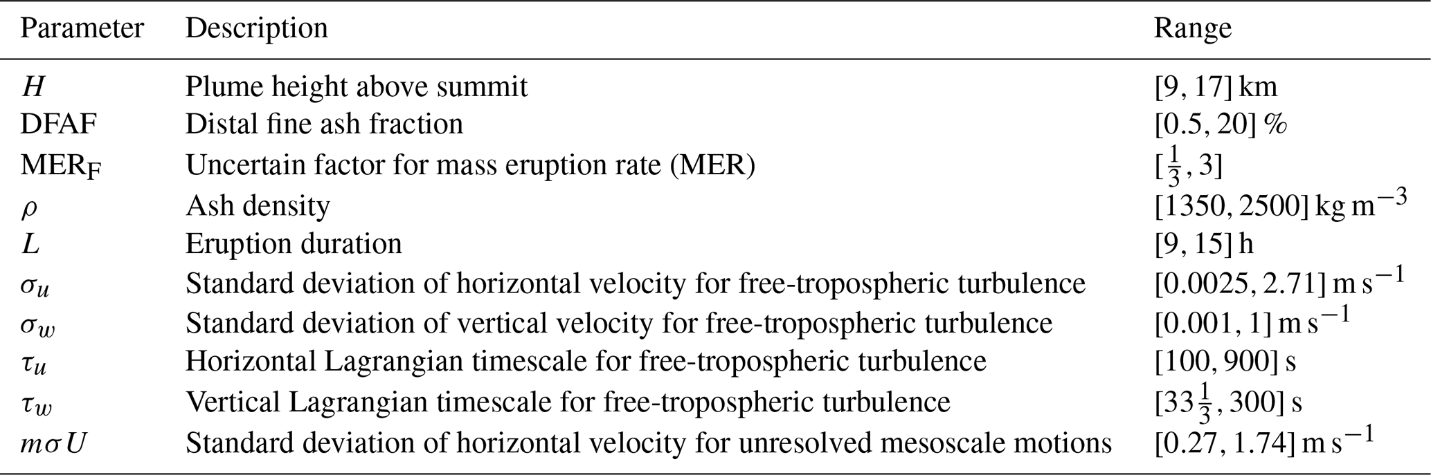
The mass eruption rate (MER) is an important driver of the model output and is calculated from the other inputs as

$$\text{MER}=\mathrm{50.7}\times {\mathrm{10}}^{\mathrm{7}}\times H^{\mathrm{1}/\mathrm{0.241}}\times {\text{MER}}_{\mathrm{F}}\times \text{DFAF},$$

where the MER_F and DFAF (distal fine ash fraction) inputs have been applied to the relationship from Mastin et al. (2009) (written here in g h⁻¹).

For each of the 1000 sets of source and internal parameters, the meteorological input is sampled from an 18-member meteorological ensemble, MOGREPS-G (members labelled 0–17), initialised at 12:00 UTC on 21 June 2019 (Bowler et al., 2008). Each input set is simulated with a single meteorological scenario. The resulting 1000-member NAME ensemble contains 30 simulations with meteorological scenarios 0 and 17 and 58–60 simulations with scenarios 1–16. Capponi et al. (2022) performed subsequent simulations based on their constrained parameter distributions; however, we restrict to the initial 1000-member space-filling design.

2.3 Observations

To enable simulations of the event to be compared to the real world, observations from the geostationary satellite Himawari-8 are used (Bessho et al., 2016). These data are available at both high temporal and high spatial resolution. Pixels are classified as either containing ash or not with the detection algorithm described in Saint (2023). The volcanic ash retrieval algorithm of Francis et al. (2012) is used to determine an estimate of ash column loading for the pixels classified as containing ash, together with an error estimate on the retrieved values. Further processing is undertaken to additionally classify pixels as clear sky and regrid to a regular latitude–longitude grid corresponding to that used for the NAME predictions with the resolution 0.45° × 0.3°. This processing is as described in Pelley et al. (2021), except that the target grid is slightly higher in resolution, and there is no averaging in time, with only the satellite data from the times indicated used.

Figure 1 plots the output of three NAME simulations at 12 h after the start of the eruption (with least, most, and close-to-average ash) compared to the equivalent satellite retrievals. The observed ash cloud may be incomplete due to failures of the detection or retrieval algorithm to either classify pixels as ash or reach an acceptable solution for the ash cloud properties. Although in some cases obscuring meteorological cloud can be an issue for the detection, most of the failures here are caused by either high ash column loadings or ash particle sizes beyond the detection algorithm's sensitivity range. Column loadings lower than approximately 0.2 g m⁻² are not usually detected by this algorithm but qualitative assessment of the satellite imagery suggests that much of the ash in the yellow regions visible from the NAME runs in Fig. 1 was not present. Note that the observations plotted here are not perfectly consistent with Capponi et al. (2022), due to use of an updated method for processing satellite observations and regridding of the observations.

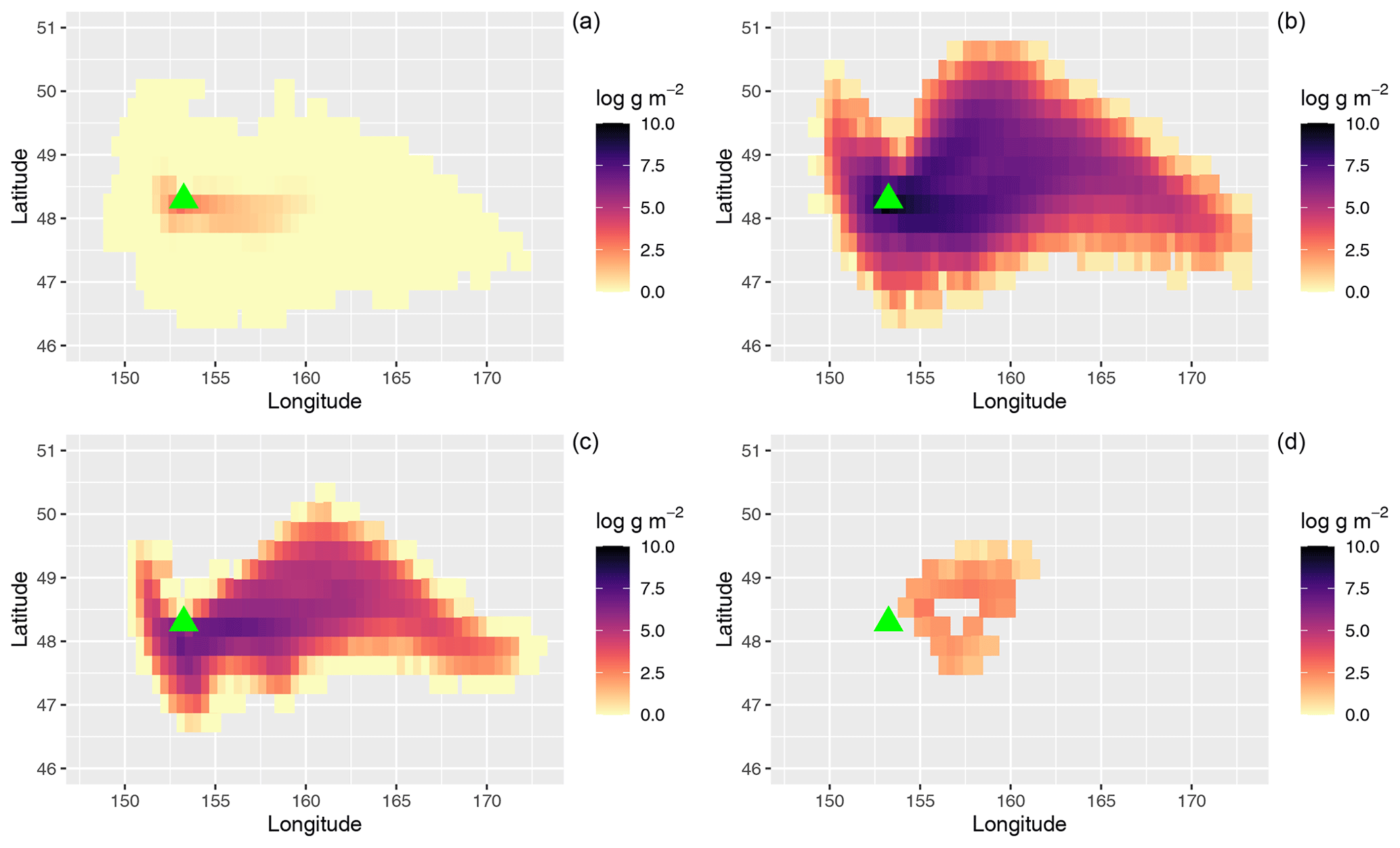
Figure 1 Predicted ash column loads (logarithm of g m⁻²) at 06:00 UTC on 22 June 2019 from three NAME simulations leading to least ash (a), most ash (b), and closest-to-ensemble-mean ash (c) and the corresponding satellite retrieval estimates (d). The green triangle indicates the location of Raikoke.

3 Methods

For clarity around the use of “model”, hereafter “simulator” will refer to NAME, and “emulator” will refer to a statistical model.

3.1 Emulation

Let the physics-based simulator (i.e. NAME) be denoted by f(⋅), which takes a vector of inputs $\mathbf{x}\in \mathcal{X}\subset {\mathbb{R}}^p$, where 𝒳 denotes the p-dimensional space of possible simulator inputs and returns output f(x). Here, x represents the values of the inputs described in Table 1 (i.e. the source inputs and internal NAME parameters), with the meteorological input ignored for now. The simulator is run for a set of n inputs $\mathbf{X}=({\mathbf{x}}_{\mathrm{1}},\mathrm{\dots },{\mathbf{x}}_n)$ for x_i∈𝒳, resulting in a set of n simulations $\mathbf{F}=\left(f\right({\mathbf{x}}_{\mathrm{1}}),\mathrm{\dots },f({\mathbf{x}}_n\left)\right)$, where each $f(\cdot )\in {\mathbb{R}}^{\mathrm{\ell }}$ is vectorised output of (or processed from) a single NAME simulation. Given a set of simulations, we fit a statistical model or “emulator” so that the simulator output can be predicted for any new input without having to run the true (expensive) simulator.

When the simulator output is a single value (or has been summarised to be a single value; for example, total mass of atmospheric ash at 06:00 UTC on 22 June 2019), i.e. ℓ=1, Gaussian processes (GPs) are a natural choice of emulator and allow fast prediction at unseen settings of x, along with uncertainty in this prediction (we have not observed the true simulator at these points), which generally increases as we move further (in input space) from known data points. In general, conditional on the n simulator runs F, we emulate f(x) as

$$\begin{array}{}\text{(1)}& f\left(\mathbf{x}\right)|\mathbf{F}\sim \text{GP}\left(\mathit{\mu }\left(\mathbf{x}\right),C\left(\mathbf{x},{\mathbf{x}}^{\prime }\right)\right),\end{array}$$

for mean function μ(x) (which may range from constant to a complex regression model in the inputs) and covariance function $C(\mathbf{x},{\mathbf{x}}^{\prime })$ (often squared exponential or Matérn), containing parameters controlling the variance, and correlation in each input dimension. The covariance may also include a “nugget” term (Andrianakis and Challenor, 2012) representing variance around training points. If this is zero, then the GP interpolates training data exactly. If this is estimated, then it may represent a number of uncertainties, including the effect of unaccounted for (inactive) inputs or stochasticity in the simulator. The nugget may be assumed to be constant across input space or dependent on x (e.g. hetGP; Binois et al., 2018).

When ℓ>1, for example, if we wish to emulate spatial, temporal, or spatiotemporal simulator output, the two main approaches are based around GPs as follows: by assuming independence and fitting GP emulators to each output independently (Lee et al., 2012) or by using a basis decomposition over the output F and emulating the coefficients given by projection onto this basis with GPs (Higdon et al., 2008; Salter et al., 2019). In what follows, we consider total ash column loads, aggregated across different regions and for different lead times (as in Harvey et al., 2018), and fit independent GP emulators to each of these summaries of the simulator output.

NAME also requires meteorological data as an input with the meteorological scenario m drawn from ℳ, some space of possible meteorologies; in this application, $\mathcal{M}=\mathit{\{}\mathrm{0},\mathrm{\dots },\mathrm{17}\mathit{\}}$ represent the 18 MOGREPS-G ensemble members (for which simulations were run by Capponi et al., 2022). Given the nature of the NAME simulations in this study, we can account for this meteorological uncertainty via emulation in two different ways.

First, we assume that NAME is stochastic with respect to m (i.e. if a NAME simulation is run at input x for different choices of m from ℳ, then the output f(x) is different). We fit a single emulator that captures the dependence due to the inputs x, and the variability across the different meteorological scenarios m. This can be approached via Eq. (1), with the nugget term representing the variability in the output at x due to m. Rather than exactly emulating any combination of (x,m), this emulates the mean of NAME at x, given any sample of m from the 18-member MOGREPS-G ensemble.

For a particular x, we can write E[f(x)],Var[f(x)] (we do not need to know m because we are not emulating or predicting for a specific m but across all m). The expectation is therefore targeting the mean of the NAME output at x, if we were to run it at all 18 meteorological inputs. The variance here accounts both for extrapolation from observed points in the input space but also for the fact that we can view f(x) at 18 different choices of m.

As a second approach, because the meteorological scenarios are sampled from a small, finite set, each of the 18 meteorological scenarios, m, could be thought of as representing a different configuration, f_m, of NAME. Each configuration gives deterministic output at input x, and we could emulate each in turn as follows:

$$\begin{array}{}\text{(2)}& f_m\left(\mathbf{x}\right)|{\mathbf{F}}_m\sim \text{GP}\left({\mathit{\mu }}_m\left(\mathbf{x}\right),C_m(\mathbf{x},{\mathbf{x}}^{\prime })\right),m=\mathrm{0},\mathrm{\dots },\mathrm{17},\end{array}$$

where F_m is the subset of F containing simulations run using meteorological input m, and the mean μ_m(⋅) and covariance $C_m(\cdot ,\cdot )$ functions are estimated for each m separately.

In this approach, for a particular summary of the NAME output, we fit a set of 18 emulators, and for any choice of x, we can predict the simulator output at this input vector for all of the 18 meteorological scenarios as follows:

$$\left(\mathrm{E}\left[f_m\left(\mathbf{x}\right)\right],\text{Var}\left[f_m\left(\mathbf{x}\right)\right]\right),m=\mathrm{0},\mathrm{\dots },\mathrm{17}.$$

The variance here only reflects the fact that we have not simulated NAME itself at all combinations of (x,m) (the emulator is extrapolating from known points).

In summary, the first approach predicts the output of NAME at x, averaged across the 18 meteorological ensemble members, and the second predicts the output for a specific combination of (x,m). The latter has the benefit that it represents NAME in a truer sense; we can query the emulator for any combination of (x,m), as with NAME itself. However, the first approach does not in general require a small ensemble of meteorological scenarios and could instead capture the uncertainty due to a more continuous set of scenarios (e.g. if every simulation of NAME was performed with a slightly perturbed meteorological input).

In Sect. 4, we consider both approaches, referring to them as the “overall” and “MET-specific” emulators, respectively.

3.2 History matching

Given an emulator(s), we may wish to compare to real-world observations of the modelled quantity and constrain the input space based on this. Often this is done via history matching (Craig et al., 1996), where we rule out clearly poor choices of the inputs, returning a space of not implausible x∈𝒳, with the retained part of 𝒳 containing inputs that may be consistent with observations, given uncertainty due to emulation, observation error, and inconsistencies between the real-world and the simulator. We assume

$$z=f\left({\mathbf{x}}^{*}\right)+e+\mathit{\eta },$$

where f(x^*) is the simulator at the “best” input x^*, which represents real-world observations z up to observation error e and model discrepancy η (differences between observations and the simulator are independent of the inputs x, e.g. due to missing or simplifications of physical processes). The simulator f(⋅) can be replaced by an emulator, and the “implausibility” of an input x is given by (Vernon et al., 2010; Williamson et al., 2013)

$$\begin{array}{}\text{(3)}& \mathcal{I}\left(\mathbf{x}\right)={\displaystyle \frac{|z-\mathrm{E}\left[f\left(\mathbf{x}\right)\right]|}{\sqrt{\text{Var}\left[f\left(\mathbf{x}\right)\right]+\text{Var}\left[e\right]+\text{Var}\left[\mathit{\eta }\right]}}},\end{array}$$

where the expectation and variance of f(x) are from an emulator (if we were able to run the simulator at any x, Var[f(x)]=0), and Var[e],Var[η] are the variance of the observational error and model discrepancy respectively. The not-ruled-out-yet (NROY) space is defined as the subset of 𝒳 where the implausibility falls below threshold T as follows:

$${\mathcal{X}}_{\mathrm{NROY}}=\left\{\mathbf{x}\in \mathcal{X}\left|\mathcal{I}\right(\mathbf{x})<T\right\},$$

with T=3 being a standard choice by the three-sigma rule (Pukelsheim, 1994).

𝒳_NROY contains settings of the inputs where, given all sources of uncertainty, we cannot say that output f(x) is inconsistent with the observed value, z. It is not guaranteed that such x produces simulator output close to z, due to emulator variance, but that we are not yet sure if it will. Initially, it may not be possible to rule out some parts of the parameter space due to high emulator variance (perhaps due to lack of training points), but we may be able to rule out these regions later by running new designs on the expensive simulator and refining emulators.

History matching is often used as an iterative procedure in this way, with the goal to zoom in on parts of 𝒳 with output consistent with z, and it can be performed for multiple outputs or summaries simultaneously (Vernon et al., 2010; Williamson and Vernon, 2013). The implausibility for all variables may be required to fall below T, but, alternatively, a more conservative definition may be used with x instead ruled out based on the kth highest implausibility at x, to protect against incorrectly discarding an input due to a single poor emulator or due to misspecified discrepancy. If emulating the entire plume rather than summaries of the output so that the observations and emulator prediction E[f(x)] are ℓ-length vectors, then the formula in Eq. (3) generalises to a distance metric across ℓ-dimensional space, with ℓ×ℓ observation error and discrepancy variance matrices. Full details, including how to efficiently history match for high ℓ, are provided in Salter and Williamson (2022).

3.3 History matching for NAME

In Sect. 4, we compare history matching for NAME modelling of the Raikoke eruption using the NAME simulator only, using different choices of emulator, and using different levels of conservatism. The overall goal is not to calibrate m; these are deemed to be possible representations of the true meteorological conditions. The aim is to calibrate the inputs relating to NAME and the eruption itself (i.e. x) while accounting for the meteorological uncertainty.

In this section, ℐ(x) (no subscript) denotes the implausibility calculated from the single emulator fitted across all meteorological scenarios (e.g. Eq. 1), and ℐ_m(x) denotes the implausibility at x for meteorology m∈ℳ calculated via emulators (Eq. 2). For any given x, we can efficiently evaluate the expectation and variance for f_m(x) for each m using the emulators and hence calculate an implausibility for each choice of m, $\left\{{\mathcal{I}}_{\mathrm{0}}\left(\mathbf{x}\right),\mathrm{\dots },{\mathcal{I}}_{\mathrm{17}}\left(\mathbf{x}\right)\right\}$. By repeatedly sampling x∈𝒳, we can use this to explore all possible combinations of (x,m) and account for uncertainties in both inputs x and meteorological scenario m simultaneously, assessing how consistent each combination of (x,m) is with observations.

Below, we outline the rationale behind each definition of NROY space that we consider. The first two rely on a random choice of m and should be broadly similar (up to using NAME vs. using an emulator for NAME), whereas the latter two account for the meteorological uncertainty via different emulators. Both aim to ensure that we do not rule out the choices of x that may in fact be correct if we were to simulate f(x) for an alternative meteorological scenario from the MOGREPS-G ensemble.

Option 1: simulator-only 𝒳_S

As a benchmark to compare the emulation approaches to, we define an NROY space, 𝒳_S, using only the 1000 NAME simulations (a similar approach to Capponi et al., 2022, but with different summaries). Therefore, in Eq. (3), we can only calculate ℐ(x) at the 1000 input vectors x that NAME has been simulated at, with E[f(x)]=f(x) and Var[f(x)]=0. The NAME output is dependent on the particular meteorological scenario that each x was run with, so that the outputs that are discarded for being too dissimilar from the observations, and hence, the posterior distributions over x may be biased by which m was randomly sampled for each simulation of NAME.

If uncertainty in the NAME output due to meteorology is small (relative to observation error), then this may not matter; however, there will always be a risk that a particular simulation f_m(x) is unrepresentative of simulations at x for some different m, and hence, this definition cannot completely capture meteorological uncertainty in the output.

Option 2: pseudo-simulator 𝒳_P

Option 1 is restrictive due to requiring simulations of NAME; however, we can approximate what this NROY space would be for other choices of x via emulation. To represent this approach, we sample x∈𝒳, sample a meteorological scenario m∈ℳ uniformly, evaluate the emulator f_m(x) for this combination of (x,m), and hence calculate ℐ_m(x). This is equivalent to defining the NROY space without accounting for the meteorological uncertainty and is akin to the approach in Capponi et al. (2022).

To remove the effect of randomly sampling m, this space can be found by evaluating ℐ_m(x) across all m∈ℳ and keeping x such that it is not inconsistent with observations for at least half of the meteorological scenarios; that is

$${\mathcal{X}}_{\mathrm{P}}=\left\{\mathbf{x}\in \mathcal{X}\left|{\mathcal{I}}_m\right(\mathbf{x})<T\text{for}\ge \mathrm{9}/\mathrm{18}m\in \mathcal{M}\right\}.$$

If x is considered not implausible for only ≤ 8 of the meteorological scenarios, then it is therefore more likely we would have run NAME for this x at one of the 10 implausible choices, and we therefore rule out this x as it is inconsistent with reality.

Option 3: overall 𝒳_O

Here, we evaluate the overall emulator (i.e. treating NAME as stochastic with respect to m so that the effect of m is accounted for within this single emulator), and hence we have a single implausibility per x that captures all uncertainties, including those due to choice of meteorological scenario:

$${\mathcal{X}}_{\mathrm{O}}=\left\{\mathbf{x}\in \mathcal{X}\left|\mathcal{I}\right(\mathbf{x})<T\right\}.$$

Option 4: conservative 𝒳_C

If a parameter choice x is implausible for one or several meteorological scenarios, it may still lead to acceptable output if we ran NAME for a different m, and so we may wish to retain that x. Therefore, we should only rule out parts of 𝒳 if all meteorological ensemble members lead to implausible simulator output at x. Conversely, we should keep any input x if it is deemed to be non-implausible for at least one meteorological ensemble member (whether this is because this combination of (x,m) leads to NAME being consistent with the observations or because the emulator variance is high enough that we cannot safely say it does not match). Therefore, here we define NROY space such that we retain x∈𝒳 if ℐ_m(x) falls below the threshold for any m∈ℳ:

$${\mathcal{X}}_{\mathrm{C}}=\left\{\mathbf{x}\in \mathcal{X}\left|{\mathcal{I}}_m\right(\mathbf{x})<T\text{for\hspace{0.17em} any}m\in \mathcal{M}\right\},$$

where the implausibility ℐ_m(x) is evaluated using the emulator for f_m(x).

4 Results

In this section, we emulate aspects of NAME output to allow a more extensive exploration of the effects that the source and internal inputs, x, and the meteorological input, m, have on the output, via the cheap-to-evaluate GP emulators. We fit emulators for different lead times and regional aggregations (Sect. 4.1) and assess whether these are accurate for NAME runs not used in the training set (Sect. 4.2) and how this changes as the time since the start of eruption increases or for more localised subsets of the output. We show that the emulators can be used to consider the distribution of output at x across all possible m (Sect. 4.3) and use this to motivate the importance of accounting for meteorological uncertainty when calibrating x. We assess the accuracy of different emulators and definitions of NROY space in an idealised setting to demonstrate performance (Sect. 4.4) before considering the satellite observations (Sect. 4.5).

4.1 Emulating summaries

Using the ensemble of 1000 NAME runs simulating the Raikoke eruption, as described in Sect. 2.2, and the emulation and calibration techniques, as described in Sect. 3, we emulate several summaries of the full NAME output. So that comparisons with observations are possible, we subset the output to grid locations at which satellite observations are available for that time point and aggregate the ash column loads across these locations only (or subsets of these). We consider three particular time points (12, 24, and 36 h after the eruption started, referred to as T1, T3, and T5, respectively, for consistency with Capponi et al., 2022) for different subsets of the observed plume.

1. Total airborne ash at T1, T3, and T5.

2. Total airborne ash at T1 split into north (N) vs. south (S) by latitude = 48.1° N.

3. Total airborne ash at T1 split into west (W) vs. east (E) by longitude = 157.7° E.

4. Total airborne ash at T1 split into four regions (NW, NE, SE, and SW) given by latitude = 48.1° N and longitude = 157.7° E.

Although VAAC forecasts only go out to 18 h, we have used longer lead times as well to demonstrate whether the emulators retain accuracy as meteorological variability increases (other eruptions may have a wider range of meteorological forecasts in the first 18 h than here, so this partly attempts to demonstrate whether the method can extend to more variable events). Splitting into different geographical regions at T1 demonstrates whether spatial variability can be captured and whether there are different effects of x and m as we consider smaller regions. This will also assess whether meteorological dependence matters at shorter forecast lead times for this eruption.

Satellite observations are given at grid box level, with median, 10th, and 90th percentiles. We perform the same aggregations as with the NAME output to allow comparisons between modelled ash and reality. To estimate uncertainty in these totals, we sum the 10th and 90th percentiles for the relevant grid boxes and, assuming Normality, calculate the variance, Var[e]. This is an overestimate, as it assumes perfect correlation and hence inflates this variance; however, the true correlation structure is unknown, and this conservative estimate is preferable to an underestimation (e.g. through assuming independent errors). As model discrepancy is unknown, we assume that this is accounted for within this inflated error variance. In history matching, if we find that we rule out all of the input space, then this suggests that we misspecified/underestimated these errors, and we should increase the discrepancy variance.

Figure 2 plots the log totals (across observed ash locations) across the 1000 runs for T1 and T5, split by which MOGREPS-G member was used as the meteorological scenario for each simulation, with the solid vertical and horizontal lines showing the median satellite observation for each metric, and the dotted lines showing 99 % intervals. There is a strong relationship for each m individually, with these slightly shifted, depending on m. Only some of the meteorological ensemble members lead to simulations in the NAME ensemble that overlap with the observations (e.g. m=1 does, but the simulations with m=16 do not match T1 and T5 totals at the observed locations simultaneously).

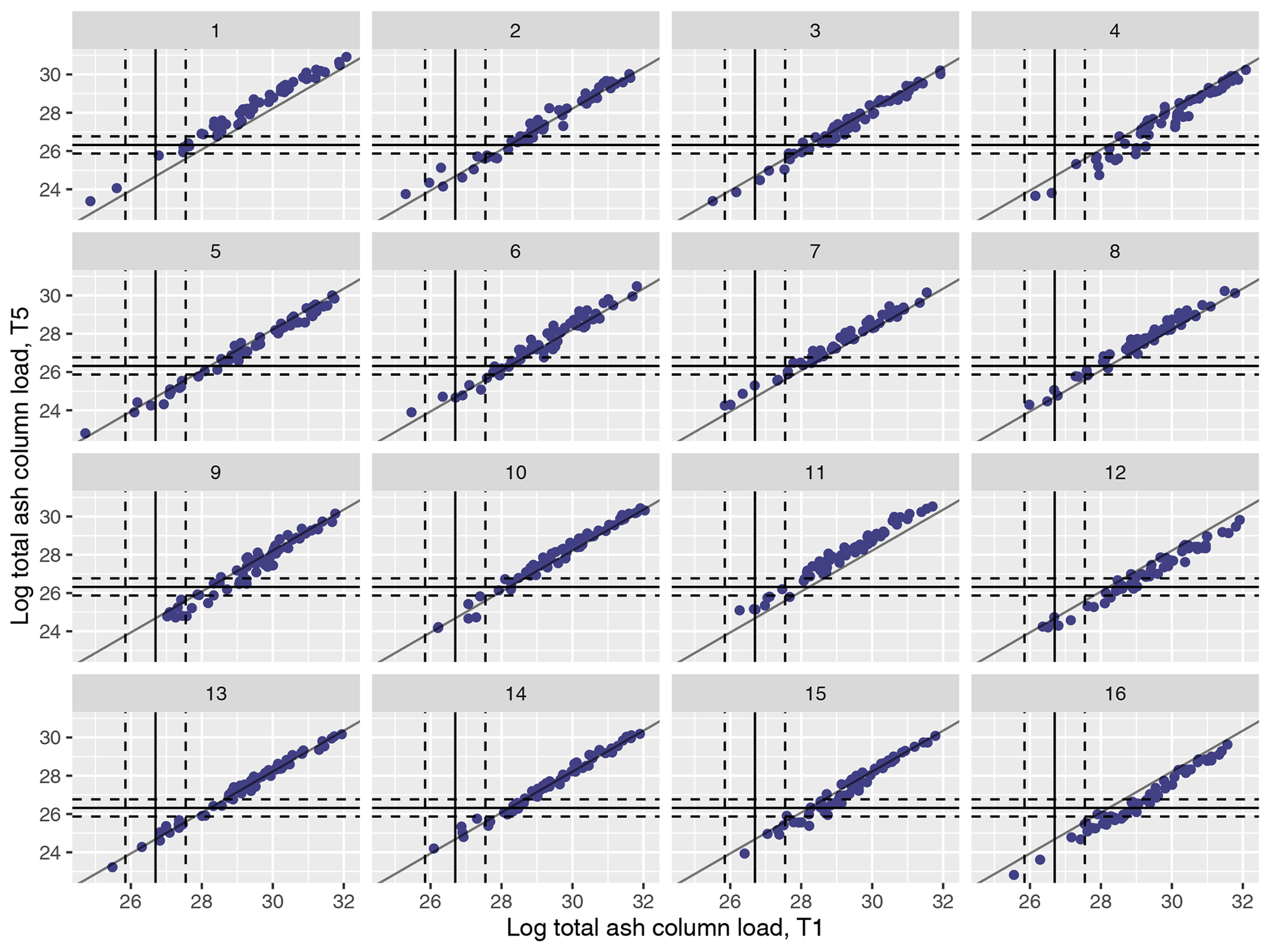
Figure 2 (Log) total ash column load (in g) in the 1000 NAME simulations aggregated across locations where ash was observed at T1 and T5 and plotted for meteorological scenarios 1–16. The vertical and horizontal lines indicate the median (solid line) and 99 % interval (dashed lines) for the satellite observations for these two time points.

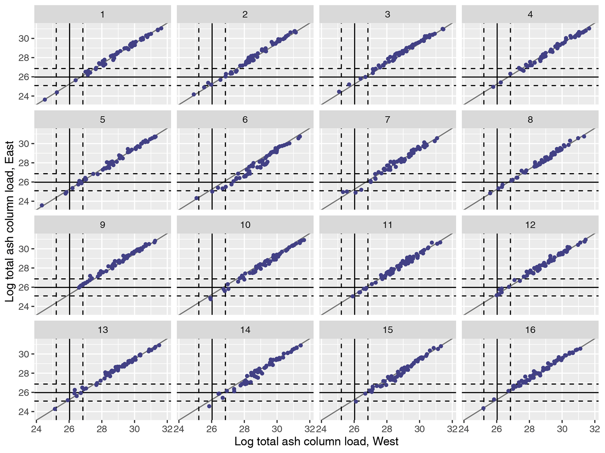
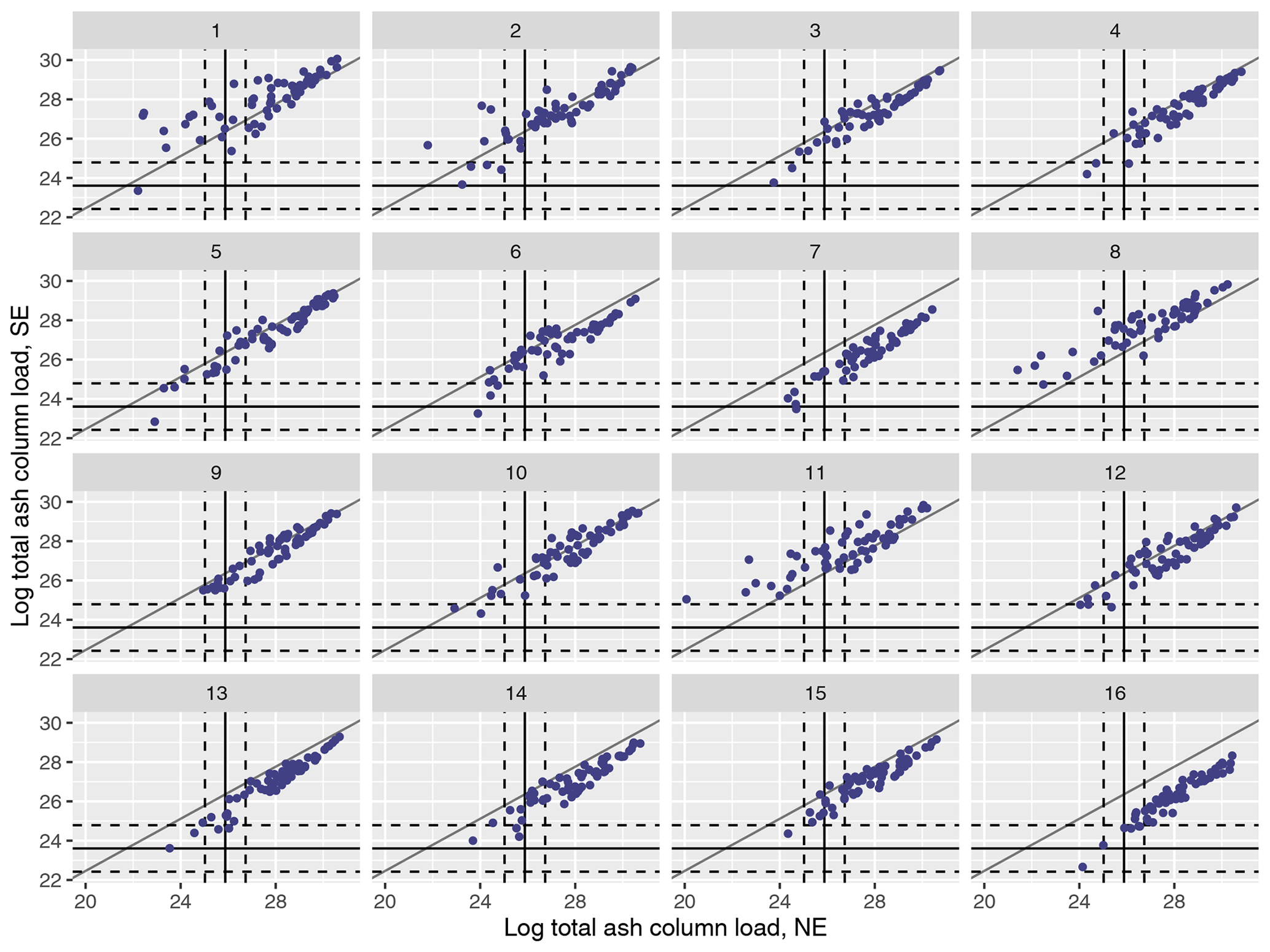
Figures 3 (north and south) and 4 (west and east) similarly plot the regional splits at T1. As before, for an individual m, there is a reasonably strong linear relationship between the two summaries; however, while this is strong and relatively similar across all m in Fig. 4, in Fig. 3 the relationship is both more noisy for an individual m and more variable between different m. This suggests that the variability in the meteorological scenarios in this case is leading to more differences in spread north/south than west/east. In each case, there are NAME simulations that lie within the 99 % interval around the satellite observations.

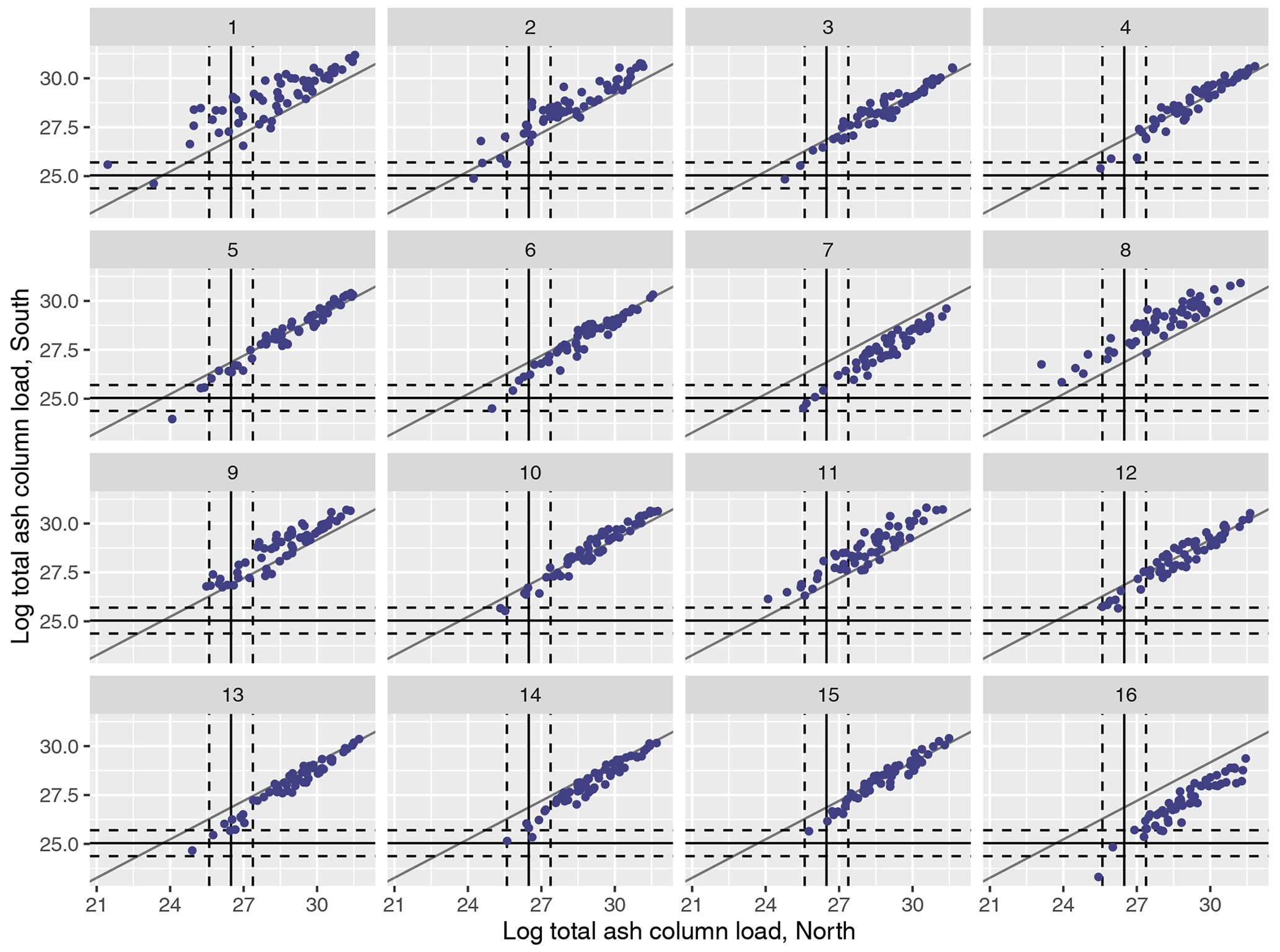
Figure 3 (Log) total ash column load (in g) for the 1000 NAME simulations for the split at T1 into north and south regions and plotted for meteorological scenarios 1–16. Median observations (solid lines) and 99 % uncertainty (dotted lines) are plotted for each regional summary.

Figure 4 As in Fig. 3 but for the west and east regions at T1.

Many of the members lie outside the satellite's uncertainty range. This is largely expected due to prior ranges leading to a wide range of possible eruptions, only sampling 1000 points in a 10-dimensional input space (not capturing all possible simulator behaviours), the NWP not being a perfect representation of weather conditions, and NAME not being a perfect simulator of an eruption, among others. However, it is worth noting that limitations in the satellite detection and retrieval algorithms that are not accounted for in the provided uncertainties likely mean that the total mass present is an underestimate, perhaps by up to an order of magnitude. If this were accounted for then slightly more members may be within the satellite uncertainty. The observed column loads are at the lower end of the 1000 NAME simulations, which is a function of the choice of prior ranges for the NAME inputs (Table 1).

For each NAME summary above, we fit the emulators described in Sect. 3.1; i.e. (1) fitting a single emulator and capturing the meteorological uncertainty within this (“overall” emulator), and (2) separate emulators trained for each meteorological ensemble member in turn (“MET-specific” emulator). In each case, we emulate the logarithm of the total ash column load and also use the log of the mass eruption rate (MER) as part of the input vector x, as ash column loads are linearly related to the emission rate.

For consistency, we split the 1000 NAME simulations into the same training (75 %) and validation (25 %) sets every time with sampling stratified by m. The overall emulator is fitted to these 750 training points, while the MET-specific emulators are trained on 22 points (MOGREPS-G ensemble members 0 and 17) or 44–45 points (all other ensemble members). In all subsequent sections, predictions for the points in the validation set are directly comparable as the same runs are always removed. Given that we already have simulations of NAME, fitting an individual emulator may take seconds (MET-specific and few training points) to several minutes (overall and 750 training points). Depending on whether the initial versions validate well, we may require repeated fittings (for example, changing the mean/covariance functions) to find a suitable emulator.

4.2 Out-of-sample predictions

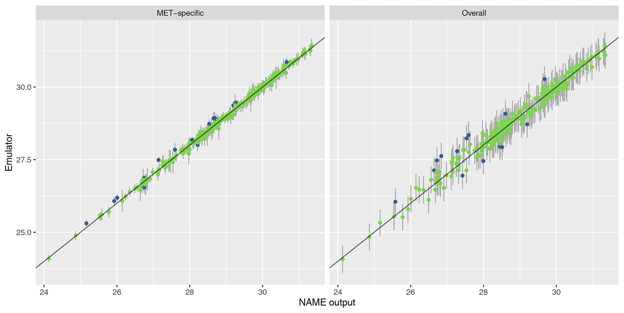
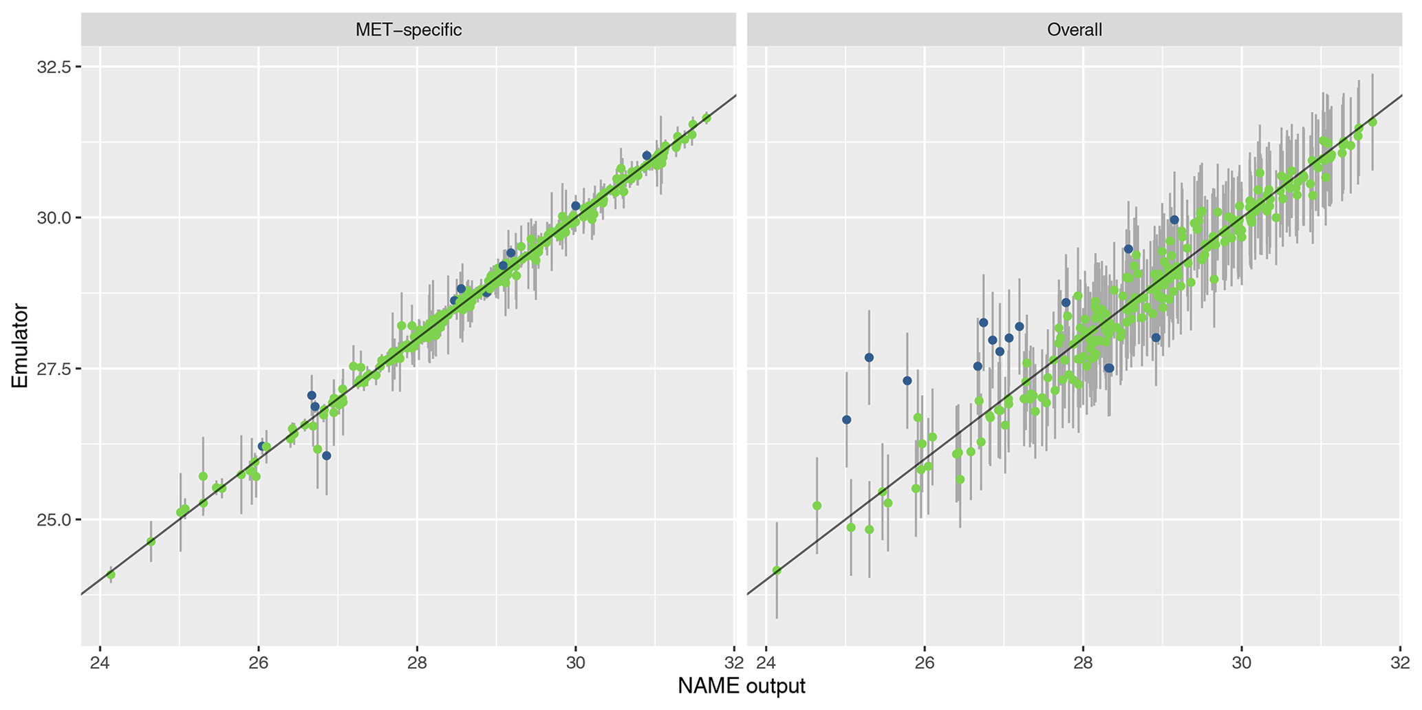
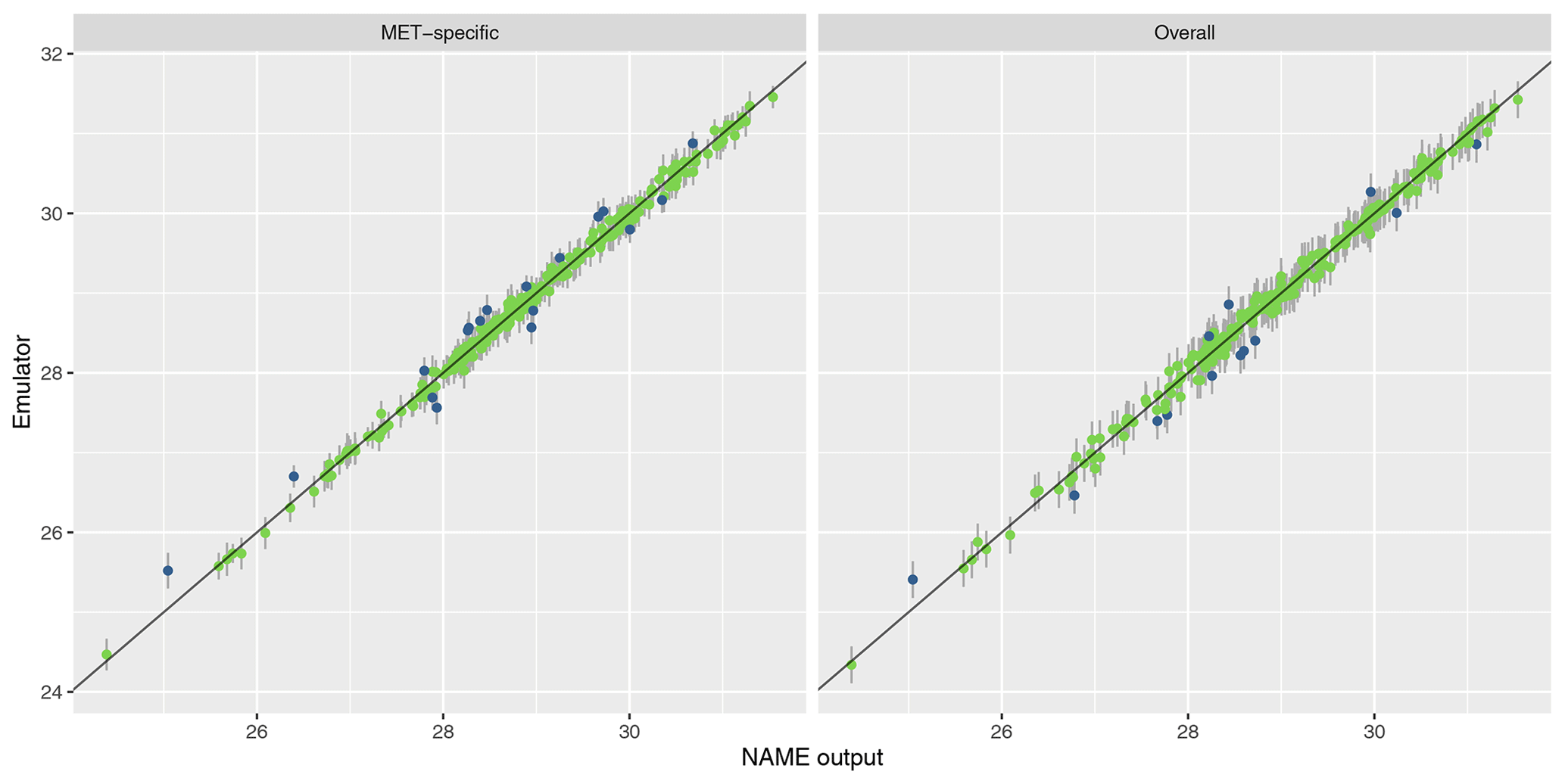
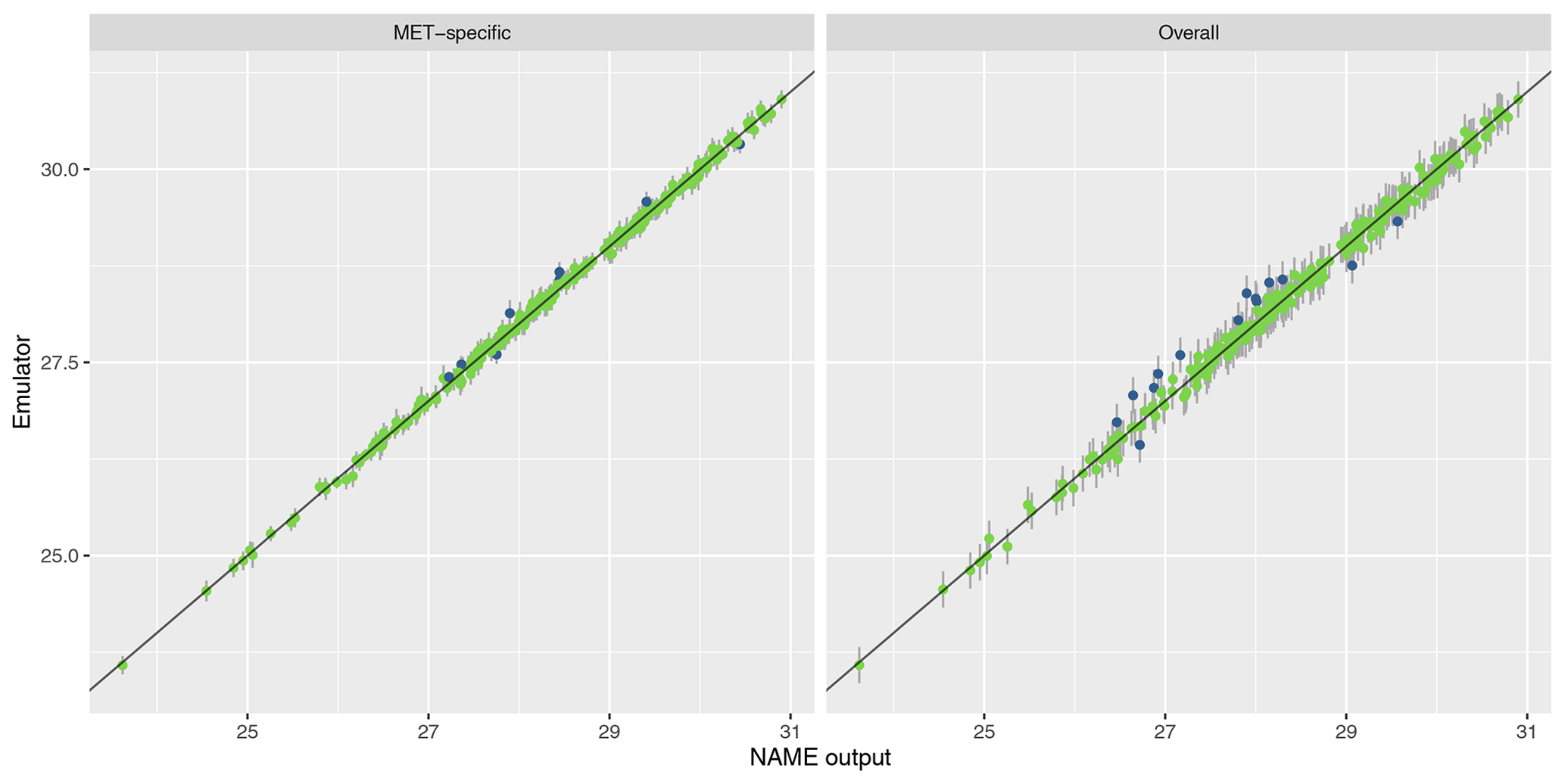
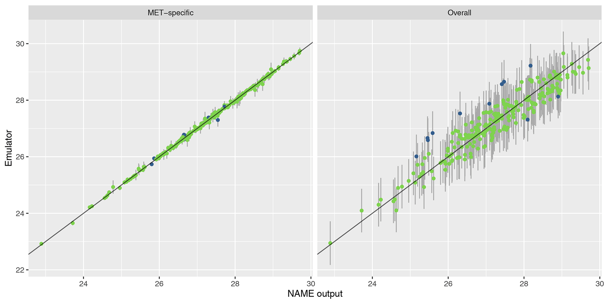
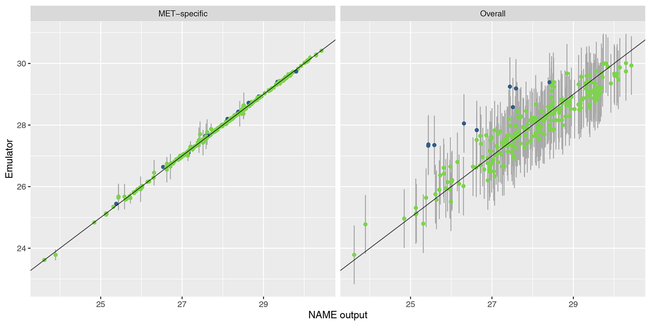
To assess emulator accuracy for the different outputs, we evaluate each emulator for the 250 points in the validation set and compare these predictions to the true NAME output. Across the fitted emulators, 93 %–97 % of the true values lie within 95 % prediction intervals, indicating that the emulators are capturing uncertainty in out-of-sample predictions well. Figures 5 and 6 plot the NAME output against emulator predictions (mean and 95 % prediction intervals) for the 250 validation points, for the totals at T1 and T5 respectively, and for the MET-specific (left) and overall (right) emulators (see the Appendix for the other emulated summaries).

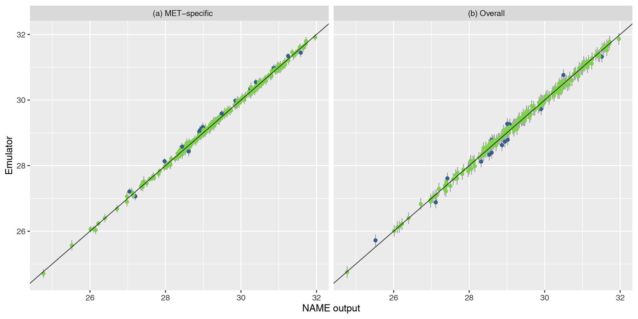
Figure 5 Out-of-sample predictions (point is for expectation; error bars show the 95 % prediction interval) plotted against NAME output for (log) total ash column load at T1 and for the MET-specific (a) and overall (b) emulators coloured by whether the true value lies within the 95 % interval (green is for true; blue is for false).

Figure 6 As in Fig. 5 but for (log) total ash column load at T5.

The error bars in the MET-specific plots account only for extrapolation via the emulator to combinations of (x,m) that were not included in the training set. The error bars in the “overall” plots account for both not training at a particular x and also the uncertainty across all meteorological scenarios. These predictions always exhibit larger uncertainty, despite the fact that the “overall” emulator is being trained with 750 points, whereas the individual m-dependent emulators are trained with at most 45 points. This indicates that, given m, dependence due to the other inputs x is predictable.

Similarly, in each case the mean predictions lie closer to the diagonal in the MET-specific cases because here we are plotting an emulator prediction for a specific m against the NAME output at that (x,m). For the “overall” plots, this compares a prediction for f(x), i.e. averaged across all meteorological scenarios, against the output for a specific m. If there is variability between running NAME for different meteorological scenarios, then the mean prediction should appear less consistent with particular NAME runs. However, as long as the particular output is generally captured within the uncertainty around this emulator prediction (which is the case around 95 % of the time), then this is not an issue, and the emulator is capturing the uncertainty due to m as intended.

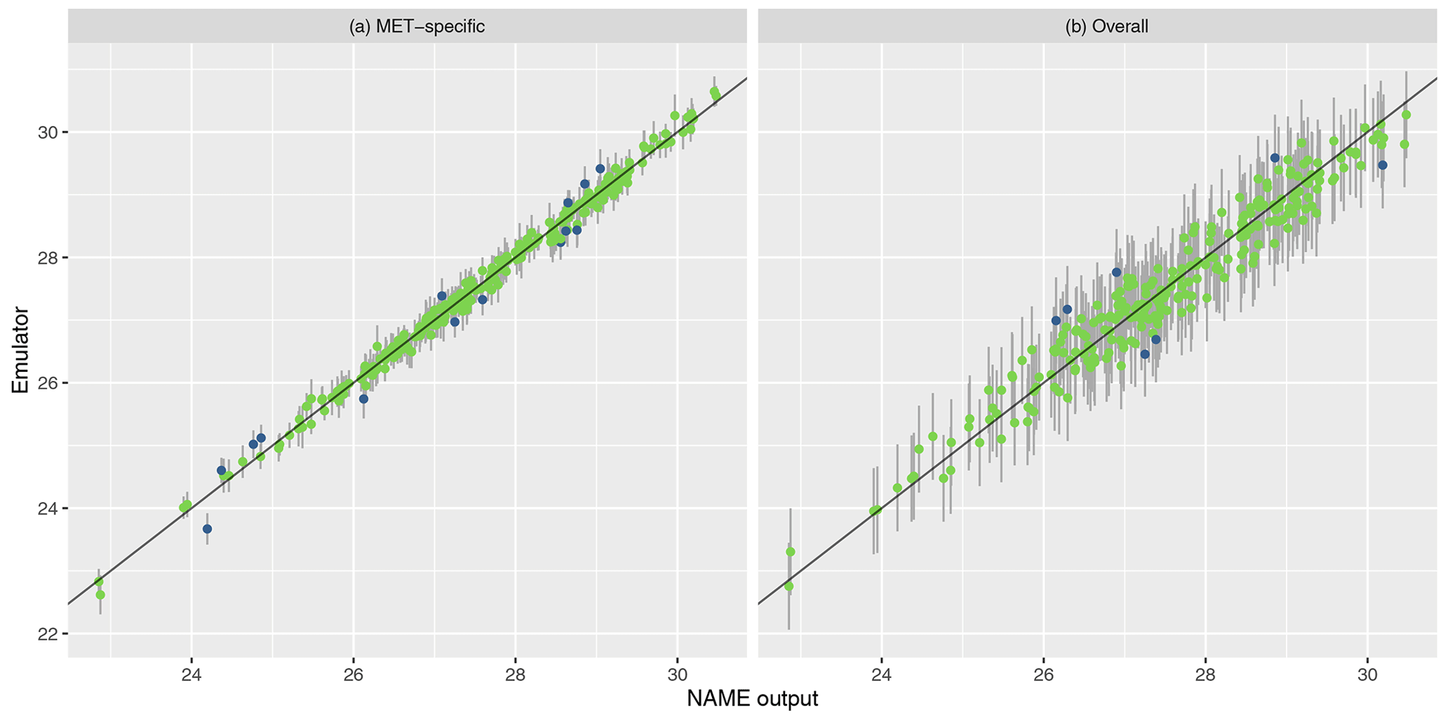
For T1, both emulators exhibit strong agreement between the emulator mean and the true NAME output. The strong correlation in the “overall” plot is therefore indicating that there is low variability in the T1 total due to the meteorological scenario (mean prediction across all m is fairly consistent with the NAME output generated by a randomly sampled m). At longer forecast lead times, we would expect that the meteorological ensemble diverges and causes greater uncertainty at a given x, and this is demonstrated by predictions at T5 (Fig. 6). The MET-specific emulators are still quite accurate (indicating that when we explicitly account for both x and m, the output is predictable), but there are larger error bars for the overall emulator, indicating that there is now a larger effect due to m.

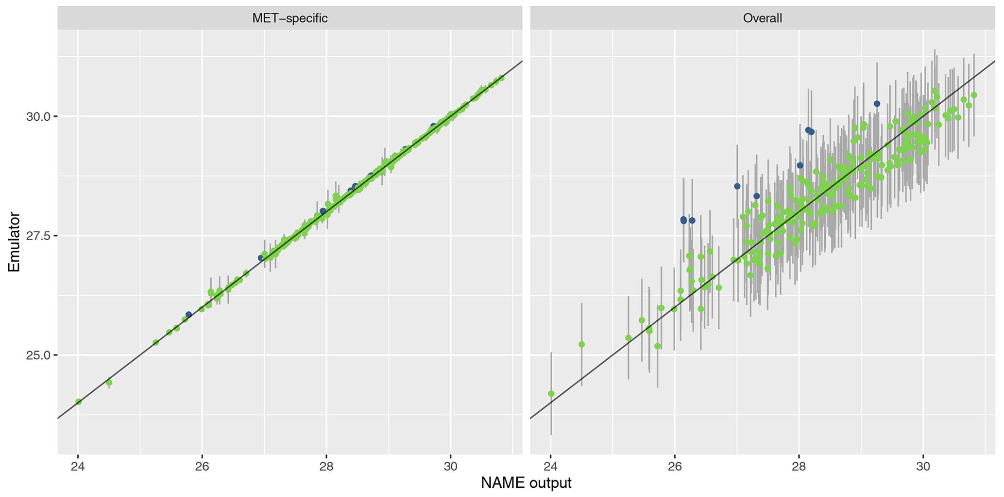
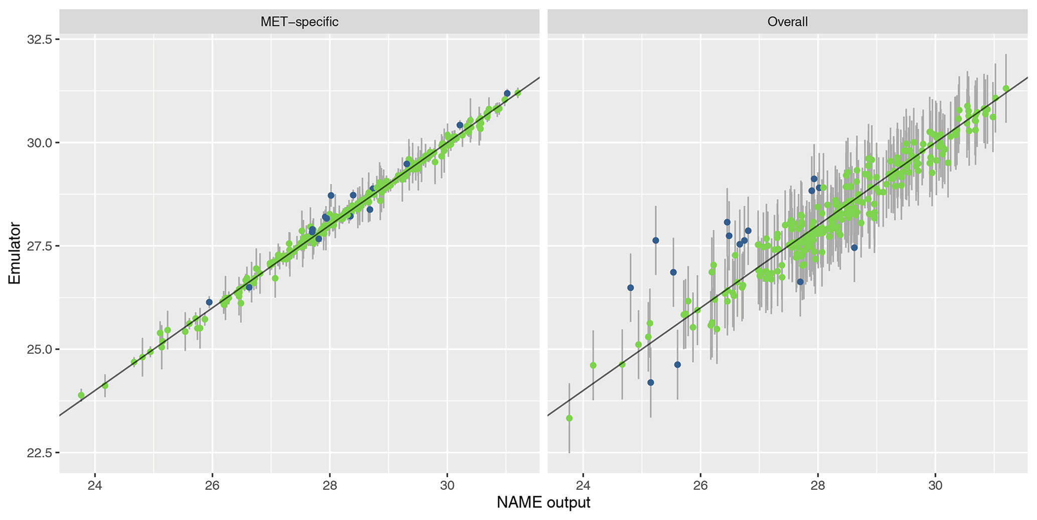
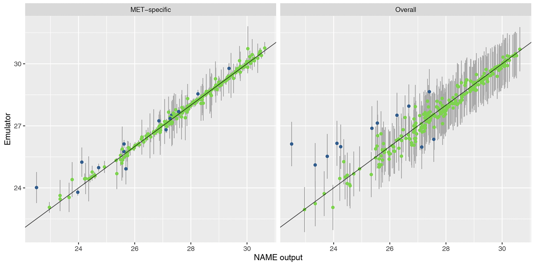
The results are similar when emulating the different regional splits at T1 (see Appendix A); the MET-specific emulators perform accurately for the north/south and west/east splits, and although they become less accurate at capturing the mean for the split into four regions, there is still predictive ability. The overall emulators validate similarly for the west and east regions (agreeing with the earlier assessment that this split did not introduce much meteorological dependence); however, there is evidence of greater effect of m with the north/south split and even more so when splitting into four regions instead.

Overall, the MET-specific emulators show that when we account for the meteorological dependence explicitly then we can accurately predict the total ash across observed locations, despite only training these emulators on a small number of inputs x. At longer lead times, or considering smaller geographical regions at T1, the overall emulator suggests that the meteorological variability is increasing; however, according to the MET-specific emulators, the joint dependence between x and m is generally retaining its predictability. This gives us a tool that can be applied to rapidly produce predictions for the Raikoke eruption across all meteorological ensemble members for any particular choice of x.

4.3 Predicting across meteorological scenarios

Given that the emulators are demonstrating predictive ability, these can be used to explore questions that are time-consuming if using only NAME. Here, we evaluate the emulators at particular choices of x across all 18 ensemble members from MOGREPS-G, explicitly giving the uncertainty in the simulator output due to m. We evaluate both the overall emulator and the 18 MET-specific emulators and visualise the effect of changing the meteorological input.

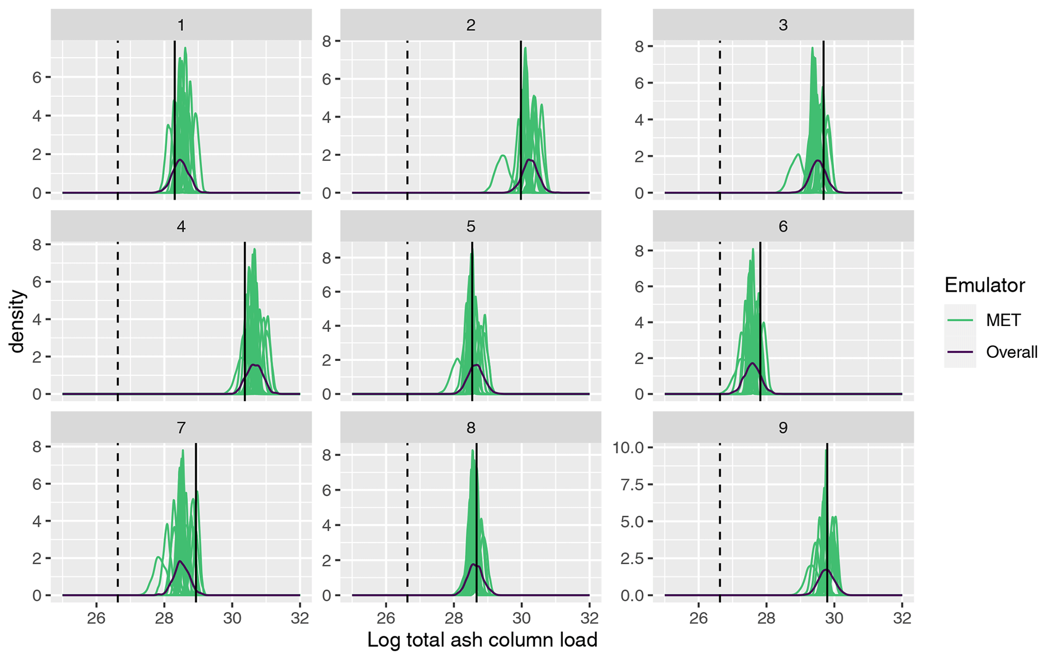
Figure 7 plots the emulator predictive distributions for the (log) total ash at T1, where x has been set as the first nine input vectors used to generate the 1000-member NAME ensemble; i.e. these were simulated with NAME using a single m, sampled at random, and the outcome of this simulation is indicated by the vertical black line in each panel. For the total at T1, the emulator predictions are relatively consistent across the 18 choices of meteorological scenario. However, at T5 (Fig. 8), there is much greater divergence in the 18 MET-specific emulator predictions at a given input x, again illustrating that there is higher variability at T5 due to m. The single overall emulator curve in each panel (dark line) has larger variance than any of the individual densities, as it is capturing the uncertainty across all m, and in each panel, we see that the overall prediction is broadly capturing the spread of the 18 individual predictions.

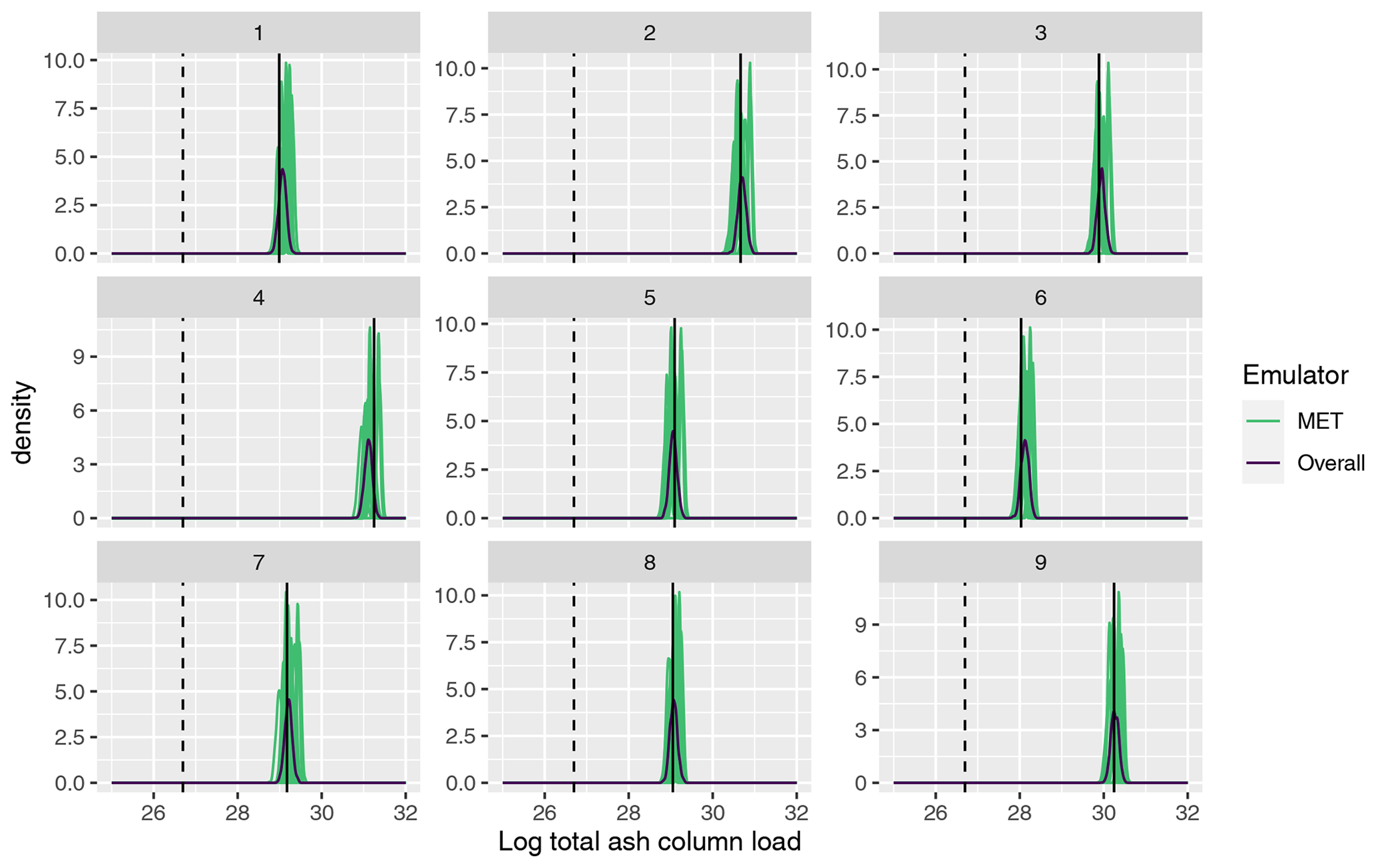
Figure 7 Emulator posteriors for (log) total ash column load at T1 evaluated across all 18 meteorological ensemble members and for the overall emulator for the first 9 design points ${\mathbf{x}}_{\mathrm{1}},\mathrm{\dots },{\mathbf{x}}_{\mathrm{9}}$ in the 1000-member ensemble. The vertical solid line indicates the value given when NAME was run at each of these 9 parameter settings (i.e. for a randomly sampled meteorology). The vertical dotted black line indicates the observed (log) total ash at T1.

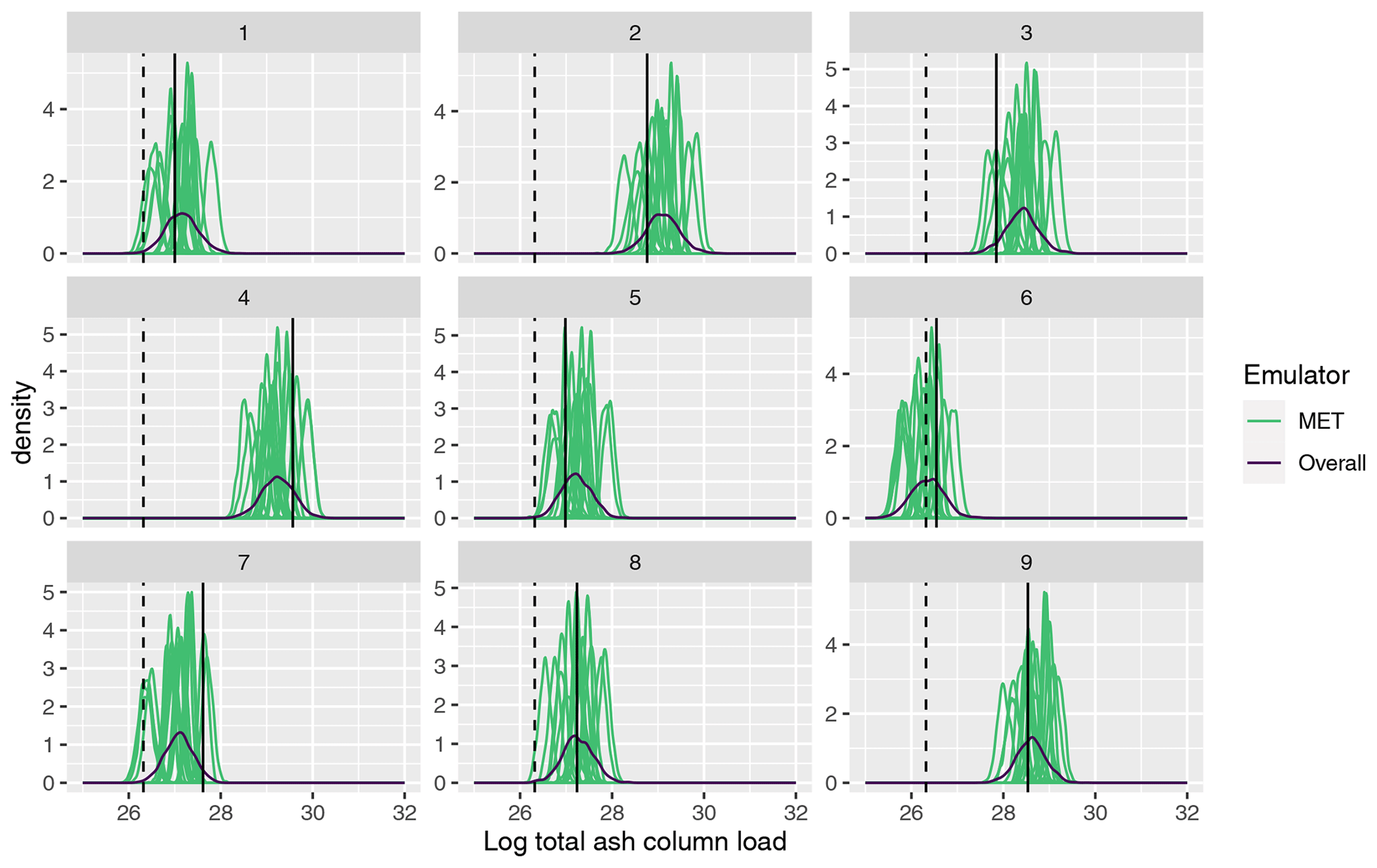
Figure 8 As in Fig. 7, comparing emulator predictions with the NAME output and observed value, but for T5.

More specifically, these plots highlight potential issues with calibration of the input parameters x. Considering panel 7 in Fig. 8, the log(total ash) value, given from simulating NAME at this design point and a sampled m, is ≈ 27.6 (vertical black line), which is away from the observed value (dashed vertical line; ≈ 26.3). Based on this comparison alone, we would likely conclude that this choice of x does not lead to NAME output that is consistent with reality. However, we see that there are two or three predictions for different choices of meteorological input that are shifted more towards the observation and that substantially overlap with this – indicating that if we had, by chance, sampled a different m at which to run this particular x, then the NAME output may have been consistent with the observation, and we would retain this x.

This example is not unique to this particular panel and this output, and it is clear that the particular m at which NAME was simulated for a given x may give a misleading representation or conclusion about that input. Particularly for T5, we see that the variability due to m is large relative to the emulator uncertainty at a particular x, and often only a small number of the distributions might intersect with the observations. The particular m we simulated NAME at may be a biased version of what we would find if we were able to run NAME at x for all 18 choices, but we will not know this by only conducting NAME runs at x for a single m. However, using the emulators, instead of a single estimate given by running NAME at a particular m, we can now predict for each m and produce a distribution for the output at input x, across all m.

4.4 History matching to pseudo-observations

In this section, we use each of the 250 NAME simulations from the validation set as “pseudo-observations”; i.e. we set $z=f\left({\mathbf{x}}^{*}\right)$ for a known x^*. We then assess whether the different emulators for NAME and different definitions of NROY space (Sect. 3.3) are able to accurately identify this true input x^*. As these simulations are taken from the validation set, in each case we are considering inputs different from what the emulators have been trained on. We consider the different emulated summaries from earlier and vary the observation error variance Var[e] (more a “tolerance to error” here). Using the emulator expectation and variance at x^* for each choice of pseudo-observations z, we can calculate ℐ(x^*) and ℐ_m(x^*) and consider the different definitions of NROY space.

We would always want the true x^* to be within NROY space – occasionally, this will not be true (some predictions always lie outside of 95 %, likewise 99 %), and it may fail if emulator prediction is biased. A large NROY space is not necessarily bad – it can signify either that our tolerance to error is large, that our emulator is relatively uncertain, or that large parts of parameter space do in fact lead to simulator output “close” to the observations – and may in fact be a realistic representation of the uncertainties in the inputs and observations.

For each choice of pseudo-observation, as a simple metric, we check whether the assumed truth x^* is retained or incorrectly ruled out. This does not give a complete picture, as perfect accuracy would be achieved by never ruling out any inputs. If emulator variance and/or observation error are large relative to the range of NAME output, then 100 % of possible inputs being considered “close enough” to the truth could be correct, but neither is true here. To provide additional information for each choice of z, we also calculate the percentage of the remaining 249 validation points that are not ruled out in each case and report the median size of this space across the 250 different choices of z (to demonstrate that any perceived accuracy is not being driven by falsely retaining all choices of x^*).

Even while knowing the input that generated the pseudo-observations, we cannot perfectly assess the accuracy of the different methods; we do not know the “true” size of each space, i.e. what percentage of input vectors would lead to output consistent with each choice of pseudo-observations, up to observation error. To do so would require evaluating x at all m∈ℳ to know whether this x is ruled out, across large samples of x, and this is not practically feasible with NAME.

We briefly outline the expected results for each definition of NROY space.

1. We do not evaluate 𝒳_S here, as it uses NAME itself, and no emulator prediction is required; hence, we always retain x^*. We also cannot evaluate whether we would retain this x^* if we would use a different m (no repeats in the NAME runs). Given accurate emulators, 𝒳_P should give a reasonable approximation of what 𝒳_S would look like if we could run many more simulations of NAME.

2. For 𝒳_P, we calculate ℐ_m(x) using the MET-specific emulators. If variability across m is low (relative to other uncertainties), then this should accurately retain x^*; however, if m has a larger effect, then we might incorrectly rule out x^*. We are effectively only allowed to view the emulator at a single m, representing running NAME once per x^* at a uniformly sampled meteorological input, which may bias inference about the inputs.

3. For 𝒳_O, we evaluate the overall emulator and explore x with m uncertain but accounted for, which should identify x^* if the meteorological uncertainty is being properly captured. The expectation of this emulator is unlikely to be consistent with the particular m that we used to generate z, and we would expect that sometimes the truth, z, lies on the edge of the posterior distribution for f(x) because we happened to view x^* at an “extreme” choice of m, and so we may sometimes rule out this input.

4. For 𝒳_C, we evaluate the MET-specific emulators and jointly explore (x,m). This space should contain x^* if the emulators are accurate – it does not matter if z was defined using a particularly extreme m, e.g. where 17 out of 18 meteorological scenarios would lead to f(x^*) being far from z; this is because we are able to explicitly consider all combinations and only require f_m(x^*) to be considered “close enough” to the pseudo-observations for a single m.

It is important to note that 𝒳_P and 𝒳_C use the same emulators, so any differences in accuracy between these two is not emulator-driven but due to the different treatment of the meteorological scenario (sampled uniformly vs. fully varied).

Table 2 shows the number of times we fail to retain the true x^*, across the 250 choices, for different NAME outputs and definition of NROY space with varied observation error. The value in the “Obs error” column refers to a scaling factor applied to the observation error variance Var[e] for the true observations. As the pseudo-observations are exactly equal to NAME output, and so there is no observational error here, this can be viewed as decreasing our tolerance to error; that is, can we find simulations closer to z, and do we still find the true x^* that generated the observations as we decrease this tolerance? N+S and W+E refer to requiring the implausibility for both emulated regions to fall below T in order to consider a point not ruled out. Similarly, “four regions” requires a point to be retained for the NW, NE, SE, and SW regions simultaneously. “At least three out of four” relaxes this, allowing one region to be considered implausible (to protect against a single biased emulator causing misclassification of inputs).

Table 2 For a given NAME output, a choice of observation error, and definition of NROY space, the table shows how often the “true” x is incorrectly ruled out when the 250 validation points in turn are taken to be the pseudo-observation. “Errors” refer to the raw number of misclassifications out of 250, and “NROY” refers to the median percentage of space that is not ruled out in each experiment.

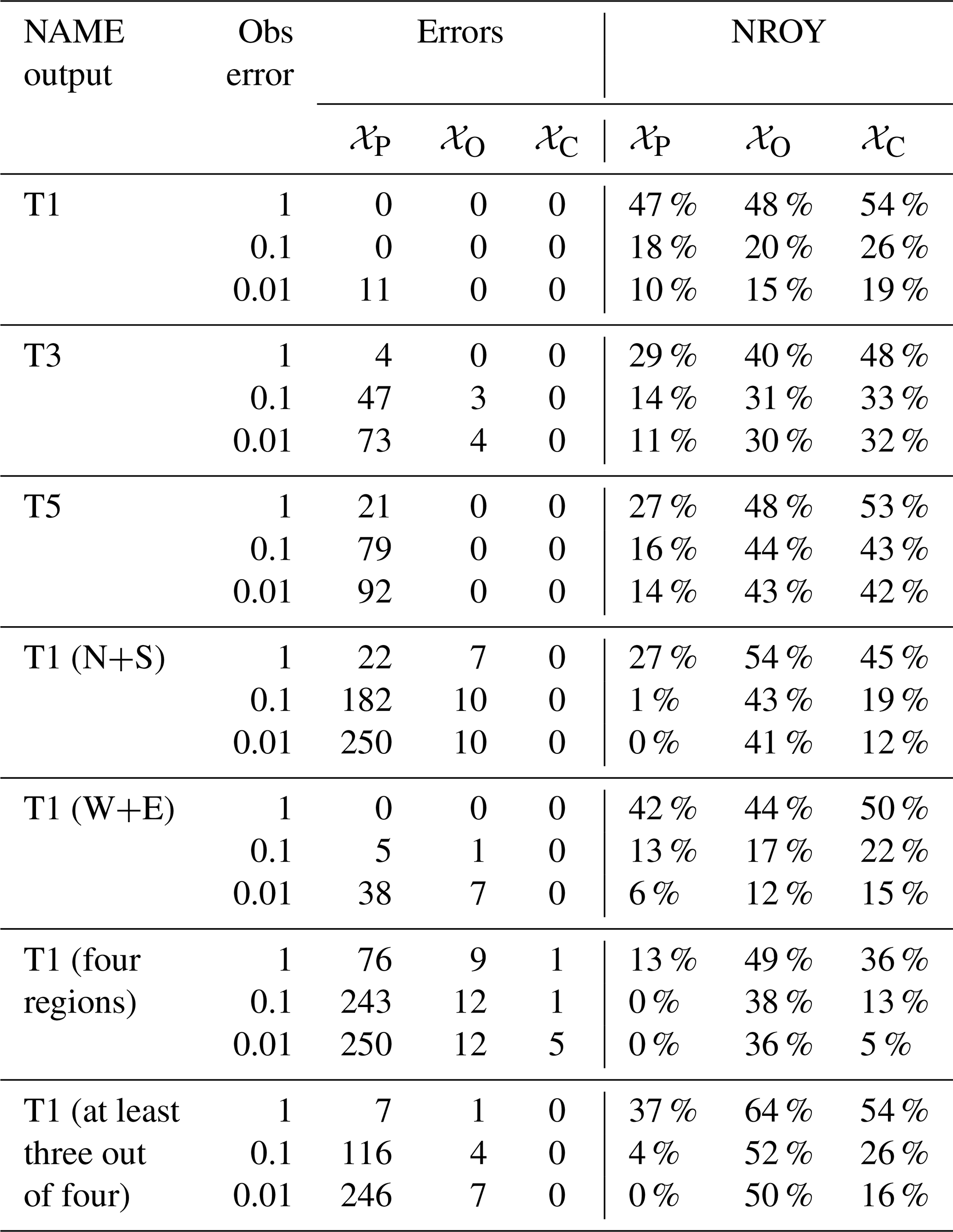
In every case, 𝒳_C performs the best in terms of retaining the true x^* and in most cases never rules out x^*, even as the error tolerance decreases. This is unsurprising, as the emulators are reasonably accurate out of sample, and this definition only rules out a parameter setting if we are confident enough that it could not be consistent with the truth for any of the 18 scenarios.

At the other end of the scale, 𝒳_P almost always performs the worst and often fails to find the true x^*. It is accurate in situations where the meteorological variability is lowest (T1 total; T1 W+E) but is poor once error tolerance reduces (e.g. even for T1, once we reduce Var[e] enough, it starts to fail) or variability across m increases (e.g. for T5, N+S split, and four-region split). Again, this result is expected – for 𝒳_P to identify x^*, it requires consistency with z across at least half of the choices of m. This is a proxy for 𝒳_S and shows that even if the true observation were generated by some known x^* and m, we would often fail to identify this x^* without accounting for the meteorological variability, and we risk incorrectly constraining the inputs.

𝒳_C and 𝒳_O generally lead to a larger percentage of the input space being retained, but it is difficult to know whether this is correct without a large number of NAME simulations. However, across different summaries and varied Var[e], we see that we rarely or never rule out the chosen x^*, even as the tolerance to error decreases and when 𝒳_P performs very poorly (suggesting larger meteorological variability relative to observation error and emulator variance). Even if bad parameter settings are not being ruled out often enough in these cases, this result is still preferable to over-constraining 𝒳 and ruling out the “correct” x^*.

Some of the examples, however, give strong evidence that the results are as intended; for the N+S split, even with the largest observation error, the true x^* is ruled out by 𝒳_P in 22 of 250 experiments and the median size of the retained parameter space across these 250 is 27 %. Even when Var[e] is 100 times smaller, 𝒳_C never rules out the true x^*, with a median of 12 % of all inputs retained; more space is being ruled out, to within a lower tolerance to error while still more accurately identifying the correct answer, thanks to evaluating all combinations of x and m.

4.5 History matching to satellite observations

Having demonstrated the accuracy of emulation and performance of the history matching definitions in an idealised setting, we now set z as the satellite observations. We have the observation error variance as before and search for (x,m), such that the NAME output is within observation error of reality. Table 3 gives the percentage of input space that is not ruled out for different combinations of the emulated outputs for each NROY definition. Unlike in the previous section, we can consider 𝒳_S here because we do not know the true input and can compare distributions derived from NAME to emulator-based ones.

Table 3 Percentage of parameter space 𝒳 that is not ruled out yet for the four different definitions of NROY space and for different individual summaries and combinations thereof. In each row, the lowest and highest percentages are highlighted by italics and bold text, respectively.

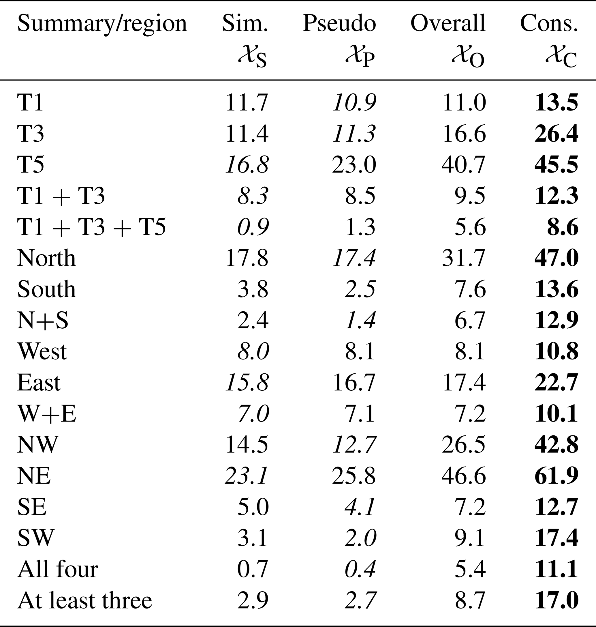
As expected, 𝒳_S and 𝒳_P usually have a similar size; the definition of 𝒳_P is such that it approximates 𝒳_S with emulation rather than only NAME simulations. Some of the differences between these two are driven by the relatively small number of samples (1000) used to define 𝒳_S, but the general similarity suggests that emulator variance is not high relative to other variability (observation error; across different inputs) and that replacing NAME with an emulator is not causing substantially more space to be retained.

𝒳_C always retains a higher percentage of the input space, and this uses the same set of emulators as 𝒳_P; hence, the increase in the percentage of 𝒳 being retained is being caused by the definition of NROY and not by the emulator uncertainty. This gives some evidence that the larger percentages of space retained by 𝒳_C may in fact be reasonable and is due to the fact that exploring more combinations (x,m) leads to the identification of substantially more possibilities for x.

Conversely, this suggests that there is a non-zero probability that 𝒳_P, and hence the simulator-only approach 𝒳_S, rules out choices of x that would in fact be considered not implausible if we happened to have simulated NAME at that x with a different sample of m. In some cases (e.g. the T1 total and the “west” region), there is not much difference in the sizes of the four spaces, which suggests that the meteorological variability is low (compared to other uncertainties) for these metrics. However, even in the most similar case (T1, with 13.5 % for 𝒳_C and 11.7 % for 𝒳_S), 1.8 %, or 18 of the 1000 runs, may have matched reality (up to observation error) if simulated at an alternative m. As in the previous section, if we consider summaries with more variability across choices of m (e.g. “south” region), the sizes diverge more, adding evidence that if we consider more local aspects of the NAME output, the impact of the meteorological scenario increases, and jointly assessing the effect of x and m is critical to ensure accurate understanding and calibration of the inputs.

The percentage of input space 𝒳 that is retained varies substantially depending on the choice of NAME output and choice of NROY definition, and observed sensitivities and relationships between different inputs are also dependent on these choices. Figures 9 (log(MER)) and 10 (mσU) plot the prior and NROY spaces for these two inputs (averaged across the other inputs) across different NAME outputs and definitions of NROY space. In each case, the distribution of log(MER) has been constrained substantially compared to the prior. For the T1 total and the split into W+E regions, the three NROY spaces are relatively similar; however, for the split into N+S and into four regions, which (from earlier) have a larger meteorological effect, there is a difference, with 𝒳_P resulting in much narrower distributions than the other definitions, while being contained within the other distributions. 𝒳_C shows that higher values of log(MER) may be possible, given the “correct” choice of m.

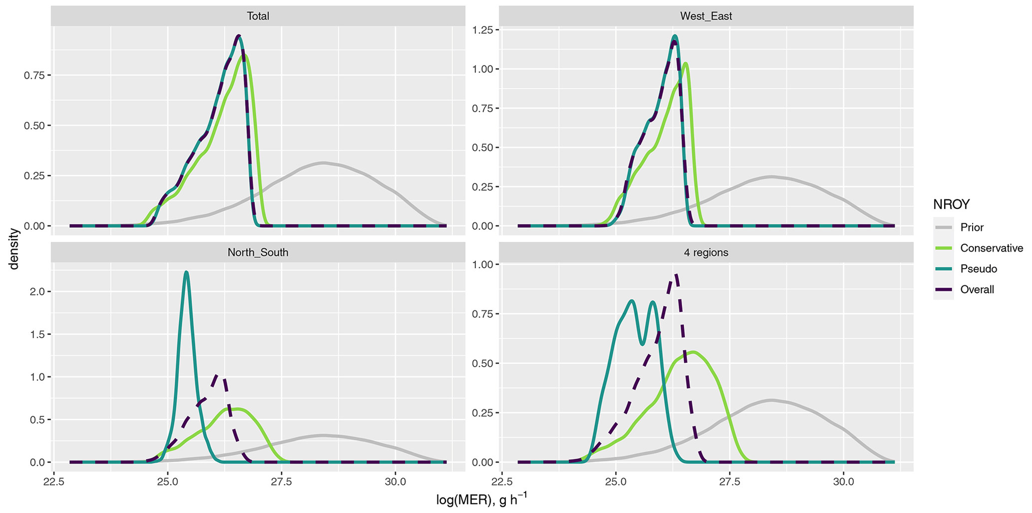
Figure 9 The distribution of log(MER), for different summaries and definitions of NROY space, compared to the prior.

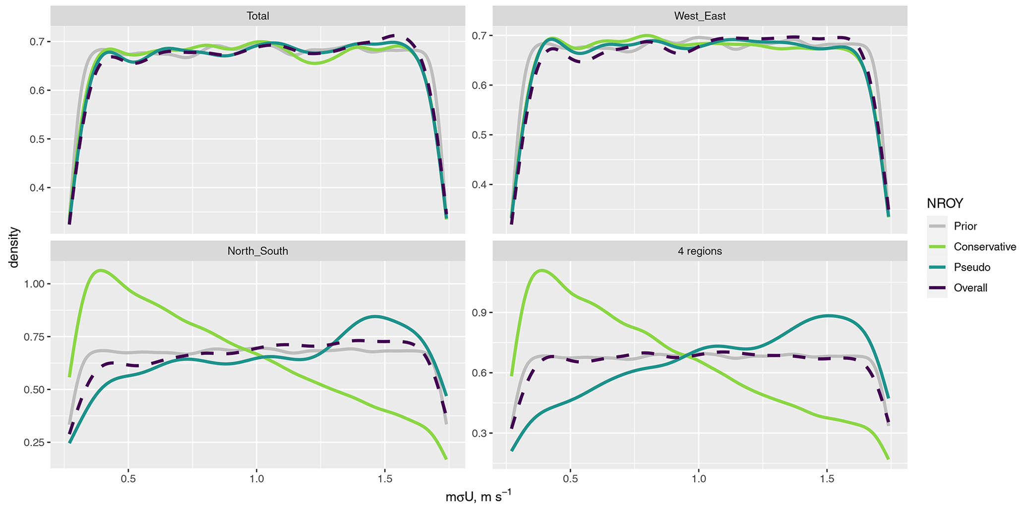
Figure 10 The distribution of mσU, for different summaries and definitions of NROY space, compared to the prior.

For mσU, regardless of the NROY definition, the posterior is the same as the prior for the T1 total and W+E split, and we might conclude that this input is not affecting the output. However, there are clearly differing results for the other regional decompositions, including the most localised summaries, and fully accounting for meteorological uncertainty leads to a strong preference for lower values of mσU. Figure 11 shows the pairwise relationship between log(MER) and mσU for the north/south regional split, for 𝒳_P, and for 𝒳_C. The opposite relationship observed for mσU in the 1D plot (Fig. 10) is due to an interaction with possible values of log(MER); 𝒳_C allows higher values of log(MER) to be considered not implausible if combined with a relatively low value of mσU.

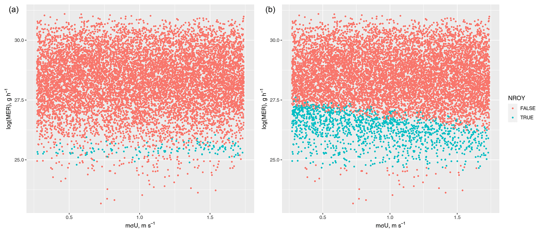
Figure 11 Pairwise representation of which combinations of log(MER) and mσU are in the 𝒳_P (a) and 𝒳_C (b) NROY spaces when history matching for the north and south regions at T1.

5 Discussion

In this paper, we have emulated different summaries of NAME output for the Raikoke 2019 eruption, simultaneously exploring the dependence on, and uncertainty due to, the eruption source inputs, the internal NAME parameters, and the meteorological scenario. We demonstrated the accuracy of these emulators and showed that we can efficiently make predictions of the NAME output for any combination of (x,m) (with uncertainty due to this being an approximation of NAME). We used these emulators to fully explore the effects and interactions that the different inputs (source, internal, and meteorological) have on the output, accounting for the uncertainties in each of these.

Given emulators, we calibrated the source and internal NAME parameters via history matching, using different outputs, emulator type, and definition of the retained (NROY) part of the input space. This demonstrated that randomly sampling the meteorological scenario (equivalently, just running NAME) leads to a much more constrained input space compared to only ruling out combinations of the source and internal inputs if they would be inconsistent with satellite observations for all 18 possible meteorological scenarios. Due to the expense of the simulator, such a comparison is not usually feasible; however, with emulators accounting for meteorological uncertainty, this can be done efficiently with the aim of ensuring that we do not incorrectly constrain the source and internal inputs due to biases from only viewing NAME at x for a single m.

For each emulated output, using a more conservative definition of the not-ruled-out-yet space unsurprisingly resulted in a larger percentage of the original parameter space being considered not inconsistent with observations. However, the use of different choices of pseudo-observations demonstrated that this appears to be more accurate, and we also showed that this larger space was not being driven by emulator uncertainty but by the uncertainty due to the meteorological input. When the meteorological effect is smaller (e.g. as for the total at T1), the different choices of NROY space are more similar. Moving further ahead in time, or splitting the output into smaller regions, the impact of the meteorological scenario increased, resulting in a larger difference in the calibration results.

The choice of NAME summary, definition of NROY space, and how the meteorology is captured, clearly affects the conclusions we make about the importance of inputs. For example, considering only the total ash, it may appear that the unresolved mesoscale parameter, mσU, is not important; however, when considering ash north and south of 48.1° N, this parameter does have an effect – and whether its distribution is skewed left or right depends on how we are accounting for meteorological uncertainty. Some differences may be driven by our choice of summary (could use other splits than at latitude 48.1° N); however, it is probable that similar differences would be evident for other outputs.

When the meteorological scenario is restricted to a small meteorological ensemble, then accurate emulators can be constructed despite a small number of training runs. However, if there are too few runs available per scenario (either if there are fewer overall NAME simulations performed or if there is a larger available ensemble of meteorological scenarios), then treating NAME as stochastic is appropriate. Although here this emulation approach and the resulting NROY definition did not capture the meteorological uncertainty as well as the MET-specific emulators, it resulted in greater accuracy than the simulator-only approach (and the emulator-based approximation of this). The benefit of the MET-specific emulators is that they are a more realistic representation of NAME; NAME is run for a specific (x,m), and this emulator predicts the output at this combination, whereas the overall one cannot. If the meteorological scenarios themselves, or key patterns from them, could be represented via dimension reduction and hence represented by a small number of coefficients, then a wider range of scenarios could be incorporated by a single emulator while still being able to predict for a specific meteorological scenario (see, e.g., Salter et al., 2022, which demonstrates jointly calibrating simulator inputs and parameters controlling spatiotemporal temperature fields).

A benefit of history matching is in its sequential nature, and this could be exploited to simplify emulation of the full plume. For example, clearly implausible combinations of inputs and meteorological scenarios can initially be ruled out based on easy-to-emulate metrics such as the total ash, and this may remove some of the wide range of behaviours observed across the full input space. Removing implausible output makes the remaining space less variable, making the plume location more consistent, and potentially enabling the spatial aspect of the plume to be emulated more easily.

Emulation may be difficult to apply in a real-time setting, as this would require unsupervised fitting of multiple statistical models and ideally requires proper validation. However, there is a benefit in assessing past eruptions and using this information about the model inputs to enhance simulation of future eruptions (e.g. to obtain better priors on uncertain inputs for NAME simulations and better understanding of which inputs are most important/sensitive in different situations). It may also provide insights into probabilistic forecasting, as the emulators can more rigorously explore tails of joint distributions across the different sources of uncertainty. Rather than considering summaries of the output, other quantities, such as ash at a particular location over time, could be emulated instead. This could be approached in a similar way as was done in this study, with emulators trained on NAME simulations and predictions made for a more complete combination of inputs and meteorological scenarios, allowing the production and assessment of more detailed information about possible impacts at important locations.

Appendix A: Additional plots

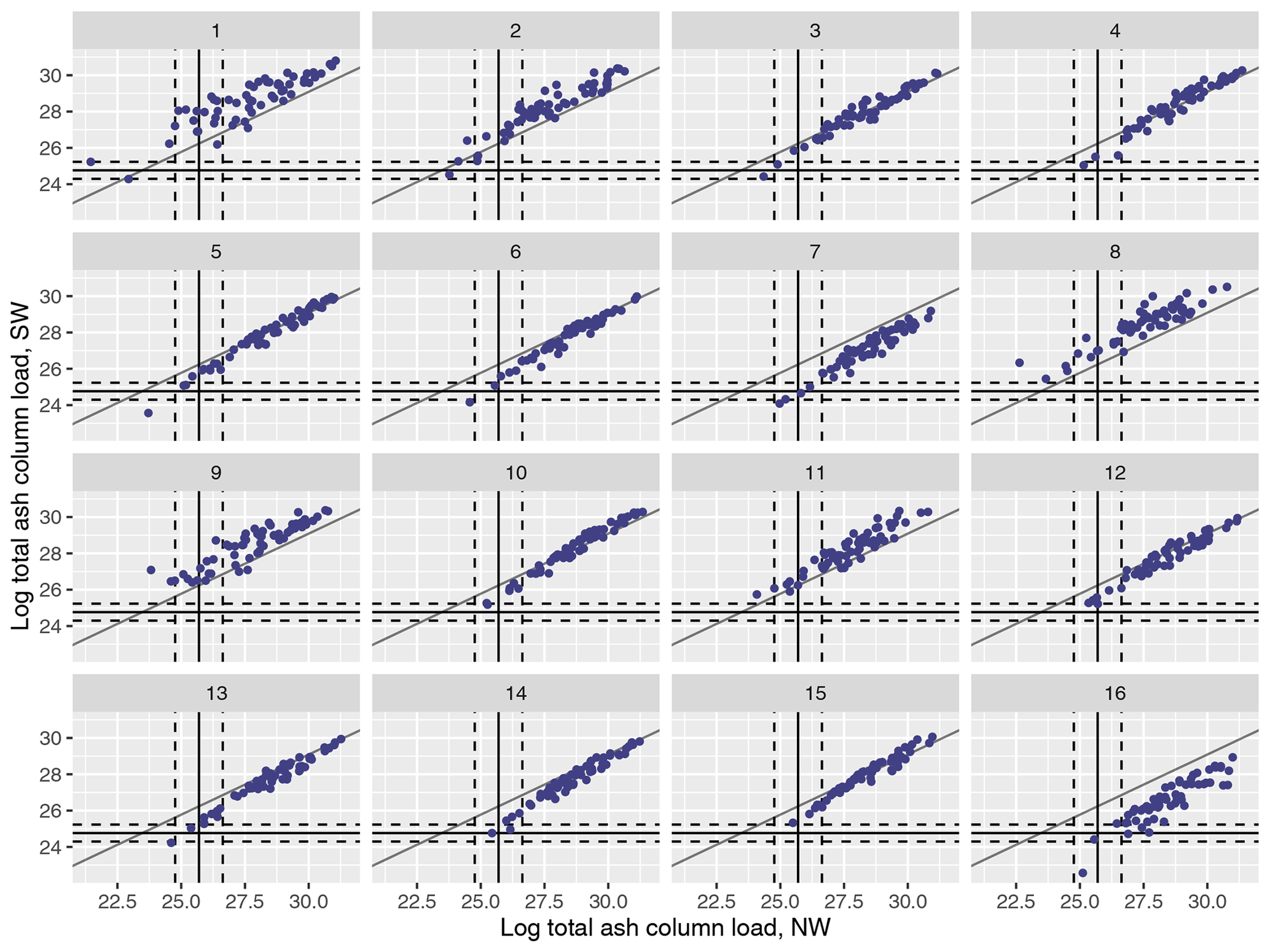
Figure A1 (Log) total ash column load (in g) for the 1000 NAME simulations and for the split at T1 into NW and SW regions and plotted for meteorological scenarios 1–16. Median observations (solid lines) and 99 % uncertainty (dotted lines) are plotted for each regional summary.

Figure A2 As in Fig. A1 but for the NE and SE regions.

A1 Validation and prediction at T3

Figure A3 Out-of-sample emulator predictions for (log) total ash column load at T3.

Figure A4 As in Fig. 7, comparing emulator predictions with NAME output and the observed value, for (log) total ash column load at T3.

A2 Validation for north vs. south split

Figure A5 Out-of-sample emulator predictions for the “north” region at T1.

Figure A6 Out-of-sample emulator predictions for the “south” region at T1.

A3 Validation for west vs. east split

Figure A7 Out-of-sample emulator predictions for the “west” region at T1.

Figure A8 Out-of-sample emulator predictions for the “east” region at T1.

A4 Validation for four-region split

Figure A9 Out-of-sample emulator predictions for the “NW” region at T1.

Figure A10 Out-of-sample emulator predictions for the “NE” region at T1.

Figure A11 Out-of-sample emulator predictions for the “SE” region at T1.

Figure A12 Out-of-sample emulator predictions for the “SW” region at T1.