Supercooled liquid water clouds observed over Dome C, Antarctica: temperature sensitivity and cloud radiative forcing

Clouds affect the Earth climate with an impact that depends on the cloud nature (solid and/or liquid water). Although the Antarctic climate is changing rapidly, cloud observations are sparse over Antarctica due to few ground stations and satellite observations. The Concordia station is located on the eastern Antarctic Plateau (75^∘ S, 123^∘ E; 3233 m above mean sea level), one of the driest and coldest places on Earth. We used observations of clouds, temperature, liquid water, and surface irradiance performed at Concordia during four austral summers (December 2018–2021) to analyse the link between liquid water and temperature and its impact on surface irradiance in the presence of supercooled liquid water (liquid water for temperature less than 0 ^∘C) clouds (SLWCs). Our analysis shows that, within SLWCs, temperature logarithmically increases from −36.0 to −16.0 ^∘C when liquid water path increases from 1.0 to 14.0 g m⁻². The SLWC radiative forcing is positive and logarithmically increases from 0.0 to 70.0 W m⁻² when liquid water path increases from 1.2 to 3.5 g m⁻². This is mainly due to the downward longwave component that logarithmically increases from 0 to 90 W m⁻² when liquid water path increases from 1.0 to 3.5 g m⁻². The attenuation of shortwave incoming irradiance (that can reach more than 100 W m⁻²) is almost compensated for by the upward shortwave irradiance because of high values of surface albedo. Based on our study, we can extrapolate that, over the Antarctic continent, SLWCs have a maximum radiative forcing that is rather weak over the eastern Antarctic Plateau (0 to 7 W m⁻²) but 3 to 5 times larger over West Antarctica (0 to 40 W m⁻²), maximizing in summer and over the Antarctic Peninsula.

1 Introduction

Antarctic clouds play an important role in the climate system by influencing the Earth's radiation balance, both directly at high southern latitudes and, indirectly, at the global level through complex teleconnections (Lubin et al., 1998). However, in Antarctica, ground stations are mainly located on the coast, and yearlong observations of clouds and associated meteorological parameters are scarce. Meteorological analyses and satellite observations of clouds can nevertheless give some information on cloud properties, suggesting that clouds vary geographically, with a fractional cloud cover ranging from about 50 % to 60 % around the South Pole to 80 %–90 % near the coast (Bromwich et al., 2012; Listowski et al., 2019). In situ aircraft measurements performed mainly over the western Antarctic Peninsula (Grosvenor et al., 2012; Lachlan-Cope et al., 2016) and nearby coastal areas (O'Shea et al., 2017) provided new insights into polar cloud modelling and highlighted sea-ice production of cloud condensation nuclei (CCN) and ice-nucleating particles (INPs) (see, for example, Legrand et al., 2016). Mixed-phase clouds (made of solid and liquid water) are preferably observed near the coast (Listowski et al., 2019) with larger ice crystals and water droplets (Lachlan-Cope, 2010; Lachlan-Cope et al., 2016; Grosvenor et al., 2012; O'Shea et al., 2017; Grazioli et al., 2017). Based on the raDAR/liDAR-MASK (DARDAR) spaceborne products (Listowski et al., 2019), it has been found that clouds are mainly constituted of ice above the continent. The abundance of supercooled liquid water (SLW; the water staying in liquid phase below 0 ^∘C) clouds depends on temperature and the liquid–ice fraction. It decreases sharply poleward and is 2–3 times lower over the eastern Antarctic Plateau than over the West Antarctic. Furthermore, the nature and optical properties of the clouds depend on the type and concentration of CCN and INPs. Bromwich et al. (2012) mention in their review paper that CCN and INPs are of various natures and large uncertainties exist relative to their origin and abundance over Antarctica. An important point remains the inability of both research and operational weather prediction models to accurately represent the clouds (especially SLW clouds, SLWCs) in Antarctica, causing biases of several tens of W m⁻² on net surface irradiance (Listowski and Lachlan-Cope, 2017; King et al., 2006, 2015; Bromwich et al., 2013) over and beyond the Antarctic (Lawson and Gettelman, 2014; Young et al., 2019). From yearlong lidar observations of mixed-phase clouds at the South Pole (Lawson and Gettelman, 2014), SLWCs were shown to occur more frequently than in earlier aircraft observations or weather model simulations, leading to biases in the surface radiation budget estimates.

Liquid water in clouds may occur in supercooled form due to a relative lack of ice nuclei for temperatures greater than −39 ^∘C and less than 0 ^∘C. Very little SLW is then expected because the ice crystals that form in this temperature range will grow at the expense of liquid droplets (called the “Wegener–Bergeron–Findeisen” process; Wegener, 1911; Bergeron, 1928; Findeisen, 1938; Storelvmo and Tan, 2015). Nevertheless, SLW is often observed at negative temperatures higher than −20 ^∘C at all latitudes, which is a danger to aircraft since icing on the wings and airframe can occur, reducing lift and increasing drag and weight. As temperature decreases to −36 ^∘C, SLW dramatically lessens, so it is highly difficult (1) to observe SLWCs and (2) to quantify the amount of liquid water present in SLWCs. But during the Year Of Polar Prediction (YOPP) international campaign, recent observations performed at the Dome C station in Antarctica of two case studies in December 2018 have revealed SLWCs with temperature between −20 and −30 ^∘C and liquid water path (LWP; the liquid water content integrated along the vertical) between 2 and 20 g m⁻², as well as a considerable impact on the net surface irradiance that exceeded the simulated values by 20 to 50 W m⁻² (Ricaud et al., 2020).

The Dome C (Concordia) station, jointly operated by French and Italian institutions in the eastern Antarctic Plateau (75^∘06^′ S, 123^∘21^′ E; 3233 m above mean sea level, m a.m.s.l.), is one of the driest and coldest places on Earth with surface temperatures ranging from about −20 ^∘C in summer to −70 ^∘C in winter. There are four main instruments relevant to this study that have been routinely running for about 10 years: (1) the H₂O Antarctica Microwave Stratospheric and Tropospheric Radiometer (HAMSTRAD; Ricaud et al., 2010a) to obtain vertical profiles of temperature and water vapour, as well as the LWP; (2) the tropospheric depolarization lidar (Tomasi et al., 2015) to obtain vertical profiles of backscatter and depolarization to be used for the detection of SLWCs; (3) an automated weather station (AWS) to provide screen-level air temperature; and (4) the Baseline Surface Radiation Network (BSRN) station to measure downward and upward longwave (4 to 50 µm) and shortwave (0.3 to 3 µm) surface irradiances (F) from which the net surface irradiance (F_Net), calculated as the difference between the downward and upward components, can be computed (Driemel et al., 2018) as

$$\begin{array}{}\text{(1)}& F_{\mathrm{Net}}=\left(F_{\mathrm{LW}}^{\mathrm{Down}}-F_{\mathrm{LW}}^{\mathrm{Up}}\right)+\left(F_{\mathrm{SW}}^{\mathrm{Down}}-F_{\mathrm{SW}}^{\mathrm{Up}}\right),\end{array}$$

where $F_{\mathrm{LW}}^{\mathrm{Down}}$, $F_{\mathrm{LW}}^{\mathrm{Up}}$, $F_{\mathrm{SW}}^{\mathrm{Down}}$, and $F_{\mathrm{SW}}^{\mathrm{Up}}$ represent the downward longwave, upward longwave, downward shortwave, and upward shortwave surface irradiances, respectively.

At a given time, the impact of a cloud on the surface irradiance is estimated from the difference between the net irradiance, in cloudy (F_Net,cld) and cloud-free (FCF_Net) conditions, to provide the so-called “cloud radiative forcing”, ΔF_Net (e.g., Stapf et al., 2020):

$$\begin{array}{}\text{(2)}& \mathrm{\Delta }{F}_{\mathrm{Net}}=F_{\mathrm{Net},\mathrm{cld}}-{\mathrm{FCF}}_{\mathrm{Net}}.\end{array}$$

A similar equation can be written for each of the four irradiances that appear in the right-hand side of Eq. (1). The aim of the present study is twofold. Using observations performed at Concordia, we intend to quantify the link between (1) temperature in the SLWCs and LWP and (2) SLWC radiative forcing and LWP.

The article is structured as follows. Section 2 presents the instruments during the period of study. In Sect. 3, we detail the methodology employed to detect the SLWCs and calculate their cloud radiative forcing, and we present the statistical method to emphasize the relationship between in-cloud temperature and LWP on the one hand and cloud radiative forcing and LWP on the other hand. The results are highlighted in Sect. 4 and discussed in Sect. 5, before concluding in Sect. 6.

2 Instruments

We have used the observations from four instruments held at the Dome C station, namely the lidar instrument to classify the cloud as SLWC, the HAMSTRAD microwave radiometer to obtain LWP and vertical profile of temperature, the AWS to obtain screen-level air temperature, and the BSRN to measure the surface irradiances ($F_{\mathrm{LW}}^{\mathrm{Down}}$, $F_{\mathrm{LW}}^{\mathrm{Up}}$, $F_{\mathrm{SW}}^{\mathrm{Down}}$, and $F_{\mathrm{SW}}^{\mathrm{Up}}$) to obtain F_Net.

2.1 Lidar

The tropospheric depolarization lidar (532 nm) has been operating at Dome C since 2008 (see http://lidarmax.altervista.org/lidar/home.php, last access: 12 January 2024). The lidar provides 5 min tropospheric profiles of clouds characteristics continuously, from 20 to 7000 m above ground level (m a.g.l.), with a resolution of 7.5 m. For the present study, the most relevant parameter is the lidar depolarization ratio (Mishchenko et al., 2000) that is a robust indicator of non-spherical shape for randomly oriented cloud particles. A depolarization ratio below 10 % is characteristic of SLWC, while higher values are produced by ice particles. The possible ambiguity between SLW droplets and oriented ice plates is avoided at Dome C by operating the lidar 4^∘ off-zenith (Hogan and Illingworth, 2003).

2.2 HAMSTRAD

HAMSTRAD is a microwave radiometer that profiles water vapour, liquid water, and tropospheric temperature above Dome C. Measuring at both 60 GHz (oxygen molecule line (O₂) to deduce the temperature) and 183 GHz (H₂O line), this unique, state-of-the-art radiometer was installed on site for the first time in January 2009 (Ricaud et al., 2010a, b). The measurements of the HAMSTRAD radiometer allow the retrieval of the vertical profiles of water vapour and temperature from the ground to 10 km height with vertical resolutions of 30 to 50 m in the planetary boundary layer (PBL), 100 m in the lower free troposphere, and 500 m in the upper troposphere–lower stratosphere. The integral along the vertical of the water vapour concentration gives the integrated water vapour (IWV). The time resolution is adjustable and has been fixed at 60 s since 2018. Note that an automated internal calibration is performed every 12 atmospheric observations and lasts about 4 min. Consequently, the atmospheric time sampling is 60 s for a sequence of 12 profiles, and a new sequence starts 4 min after the end of the previous one. The temporal resolution on the instrument allows for detection and analysis of atmospheric processes such as the diurnal evolution of the PBL (Ricaud et al., 2012) and the presence of clouds and diamond dust (Ricaud et al., 2017), together with SLWCs (Ricaud et al., 2020). In addition, the LWP (g m⁻²) that gives the amount of liquid water integrated along the vertical can also be estimated. Observations of LWP were performed when the instrument was installed at the Pic du Midi station (2877 m a.m.s.l., France) during the calibration/validation period in 2008 prior to its setup in Antarctica in 2009 (Ricaud et al., 2010a) and during the Year Of Polar Prediction (YOPP) campaign in summer 2018–2019 (Ricaud et al., 2020). At the present time, it has not yet been possible to compare HAMSTRAD LWP retrievals with observations from other instruments, neither at the Pic du Midi nor at Dome C stations. To better evaluate its performance, the 2021–2022 and the future 2022–2023 summer campaigns are dedicated to in situ observations of SLWCs. Comparisons with numerical weather prediction models were showing consistent amounts of LWP at Dome C when the partition function between ice and liquid water was favouring SLW for temperatures less than 0 ^∘C (Ricaud et al., 2020). Note that microwave observations at 60 and 183 GHz are not sensitive to ice crystals. This has already been discussed in Ricaud et al. (2017) when considering the study of diamond dust in Antarctica. As a consequence, possible precipitation of ice, within or below SLW clouds, as detected by the lidar, does not affect the retrievals of temperature, water vapour, and liquid water.

2.3 AWS

An American automated weather station (AWS) is installed at Concordia about 500 m away from the station and can provide screen-level air temperature (T_a) every 10 min. Data are freely available at https://amrc.ssec.wisc.edu/data/archiveaws.html (last access: 12 January 2024).

2.4 BSRN

The BSRN sensors at Dome C are mounted at the Astroconcordia/Albedo-Rack sites, with upward- and downward-looking, heated, and ventilated Kipp&Zonen CM22 pyranometers and CG4 pyrgeometers providing measurements of hemispheric downward and upward broadband shortwave (SW, 0.3 to 3 µm) and longwave (LW, 4 to 50 µm) horizontal irradiances at the surface, respectively. These data are used to retrieve values of net surface irradiances. All these measurements follow the rules of acquisition, quality check, and quality control of the BSRN (Driemel et al., 2018).

2.5 Period of study

From the climatological study presented in Ricaud et al. (2020), the SLWCs are mainly observed above Dome C in summer, with a higher occurrence in December than in January: 26 % in December against 19 % in January, representing the percentage of days per month that SLW clouds were detected during the YOPP campaign (summer 2018–2019) within the lidar data for more than 12 h d⁻¹. We have thus concentrated our analysis on December and the 4 years, 2018–2021. Since we have to use the four datasets (lidar, HAMSTRAD, AWS and BSRN) in time coincidence, the actual number of days per year and the time sampling for each day selected in our analysis are detailed in Table 1.

Table 1 Cloud-free periods in December 2018–2021 detected from the lidar depolarization observations at Concordia. Time is in UTC. MM-NN means from MM (included) hour UTC to NN (excluded) hour UTC. “X” means no cloud-free period during that day. “ND” means no lidar data available. Bold cases mean that cloud-free irradiance calculations are impossible due to lack of some data (lidar, HAMSTRAD, BSRN, or AWS).

3 Methodology

3.1 SLWC detection

Consistent with Ricaud et al. (2020), we use lidar observations to discriminate between SLW and ice in a cloud. High values of lidar backscatter coefficient (β>100β_mol, with β_mol the molecular backscatter) associated with very low depolarization ratio (<5 %) signify the presence of an SLWC, whilst a high depolarization ratio (>20 %) indicates the presence of an ice cloud or precipitation. Once the SLWC is detected both in time and altitude, the temperature (T) profile within the cloud and the LWP measured by the HAMSTRAD radiometer in time coincidence are selected, together with the surface irradiances observed by the BSRN instruments.

The lidar profiles are interpolated along the temperature vertical grid and then according to the temperature time sampling. As a consequence, for a given time and height, we have a depolarization ratio, a backscatter value, and a temperature, as well as (not height-dependent) IWV and LWP values. BSRN irradiances are time interpolated to be coincident with the other parameters. So, for a given time, we have a set of BSRN irradiances ($F_{\mathrm{LW}}^{\mathrm{Down}}$, $F_{\mathrm{LW}}^{\mathrm{Up}}$, $F_{\mathrm{SW}}^{\mathrm{Down}}$, $F_{\mathrm{SW}}^{\mathrm{Up}}$, and F_Net) and an LWP. At a (time, height) point showing high backscatter signal and low depolarization, the associated parameters (temperature, LWP and irradiances) are flagged as “SLW cloud”. The statistic is thus done using all the SLW-flagged points without any averaging. The temperature corresponds to the in-cloud temperature.

Figure 1 shows, as a typical example, the time evolution of the lidar backscatter coefficient and depolarization ratio, as well as the HAMSTRAD LWP and temperature vertical profile for 27 December 2021. Associated with the SLWCs, the LWP values are between 1.0 and 3.0 g m⁻². The SLWCs are present over a temperature range varying from about −28.0 to −33.0 ^∘C. Note the cloud present at 04:00–05:00 UTC that is not labelled as a SLWC but rather as an ice cloud (high backscatter and high depolarization signals) with no associated increase of LWP and temperature above −28.0 ^∘C.

Figure 1 (a–d) Time evolution (UTC, hour) of the lidar backscattering signal, the lidar depolarization signal, the HAMSTRAD LWP, and the HAMSTRAD temperature profile measured on 27 December 2021. The time evolution of the SLW cloud (as diagnosed by a backscattering value > 60 A.U. and a depolarization value <5 %) is highlighted by the red and grey areas in (c) and (d), respectively. The height above the ground is shown in (c), with the y axis on the right. The 00:00 and 12:00 local times (LT) are highlighted by two vertical dashed lines.

Figure 2 highlights the time evolution of the SLWC obtained on 27 December 2021, together with some snapshots from the HALO-CAM video camera taken with or without SLWC at 01:00 (no SLWC), 07:19 (SLWC), 09:00 (no SLWC), 10:14 (SLWC), 13:00 (no SLWC), 16:03 (SLWC), 18:01 (no SLWC), and 20:53 UTC (SLWC). SLWCs (high backscatter and low depolarization signals) are clearly detected at 07:00–08:00, 10:00–11:00, 16:00–17:00, 21:00–22:00, and 23:00–24:00 UTC over an altitude range of 500 to 1000 m a.g.l. In general, SLWCs observed over the station did not correspond to overcast conditions.

Figure 2 (a) Time evolution (UTC, hour) of the SLWC (red areas) on 27 December 2021. (b, from left to right) Snapshots from the HALO-CAM video camera taken at 01:00 (no SLWC), 07:19 (SLWC), 09:00 (no SLWC), 10:14 (SLWC), 13:00 (no SLWC), 16:03 (SLWC), 18:01 (no SLWC), and 20:53 UTC (SLWC). The 00:00 and 12:00 local times (LT) are highlighted by two vertical dashed lines.

3.2 Cloud radiative forcing

From Eq. (2), one of the main difficulties in computing the cloud radiative forcing (ΔF_Net) is to estimate FCF_Net from its individual components, namely the cloud-free downward longwave, upward longwave, downward shortwave, and upward shortwave surface irradiances. We performed several studies (reference irradiances measured over days when clouds are absent, radiative transfer calculations) from which it resulted that the most robust method was to use a parameterization of the cloud-free downward longwave and shortwave surface irradiances widely used in the community. In Dutton et al. (2004), cloud-free downward shortwave surface irradiance (${\mathrm{FCF}}_{\mathrm{SW}}^{\mathrm{Down}}$) is parameterized as

$$\begin{array}{}\text{(3)}& {\mathrm{FCF}}_{\mathrm{SW}}^{\mathrm{Down}}=a\cos (z{)}^b{c}^{\left(\frac{\mathrm{1}}{\cos \left(z\right)}\right)},\end{array}$$

where z is the solar-zenith angle, and a, b, and c are coefficients optimized using well-identified cloud-free situations. In Dupont et al. (2008), cloud-free downward longwave surface irradiance (${\mathrm{FCF}}_{\mathrm{LW}}^{\mathrm{Down}}$) is parameterized as

$$\begin{array}{}\text{(4)}& {\mathrm{FCF}}_{\mathrm{LW}}^{\mathrm{Down}}={\mathit{\epsilon }}_{\mathrm{a}}\mathit{\sigma }{T}_{\mathrm{a}}^{\mathrm{4}},\end{array}$$

where T_a is the screen-level air temperature in kelvin (K), σ Stefan–Boltzmann's constant, and ε_a the apparent atmospheric emissivity. The latter is supposed to be a function of the integrated water vapour (IWV) following the equation

$$\begin{array}{}\text{(5)}& {\mathit{\epsilon }}_{\mathrm{a}}=\mathrm{1}-\left(\mathrm{1}+\mathrm{IWV}\right)\exp (-(d+e\times \mathrm{IWV}{)}^f),\end{array}$$

where d, e, and f are coefficients that need to be optimized using cloud-free situations, and IWV is provided by the HAMSTRAD measurements. The cloud-free upward shortwave surface irradiance (${\mathrm{FCF}}_{\mathrm{SW}}^{\mathrm{Up}}$) is evaluated from ${\mathrm{FCF}}_{\mathrm{SW}}^{\mathrm{Down}}$ with the surface albedo ($A_{\mathrm{BSRN}}=F_{\mathrm{SW}}^{\mathrm{Up}}\left(\mathrm{BSRN}\right)/F_{\mathrm{SW}}^{\mathrm{Down}}\left(\mathrm{BSRN}\right))$ calculated from observations:

$$\begin{array}{}\text{(6)}& {\mathrm{FCF}}_{\mathrm{SW}}^{\mathrm{Up}}=A_{\mathrm{BSRN}}\times {\mathrm{FCF}}_{\mathrm{SW}}^{\mathrm{Down}},\end{array}$$

where $F_{\mathrm{SW}}^{\mathrm{Up}}\left(\mathrm{BSRN}\right)$ and $F_{\mathrm{SW}}^{\mathrm{Down}}\left(\mathrm{BSRN}\right)$ are the upward and downward shortwave surface irradiance measured by the BSRN instruments, respectively. With this method, we take into account the actual shape of the surface and, in particular, its rough structure caused by the sastrugi (see Sect. 5.5). Thus, the surface albedo varies with the sun angles (azimuthal and zenithal) and cannot be considered constant over the diurnal cycle.

The cloud-free upward longwave radiation (${\mathrm{FCF}}_{\mathrm{LW}}^{\mathrm{Up}}$) is evaluated as

$$\begin{array}{}\text{(7)}& {\mathrm{FCF}}_{\mathrm{LW}}^{\mathrm{Up}}={\mathit{\epsilon }}_{\mathrm{s}}\mathit{\sigma }{T}_{\mathrm{s}}^{\mathrm{4}}+(\mathrm{1}-{\mathit{\epsilon }}_{\mathrm{s}}){\mathrm{FCF}}_{\mathrm{LW}}^{\mathrm{Down}},\end{array}$$

where T_s is the surface temperature, and the surface emissivity ε_s is assumed constant and equal to 0.99. T_s is diagnosed based on Eq. (7) using the BSRN upward and downward longwave surface irradiances.

Cloud-free situations are detected based on visual inspection of the lidar (depolarization) measurements. Depolarization ratios greater than about 1 % are attributed to the presence of cloud (cirrus, mixed-phase, SLW), diamond dust, and fog, etc. Thus, within each 24 h slot covering the month of December in the years 2018–2021, the 1 h periods when the depolarization ratios are less than 1 % are considered cloud-free periods. Consequently, to evaluate the surface cloud-free irradiances over the month of December and the years 2018–2021, we need to have coincident observations from the four BSRN instruments, the lidar (depolarization), HAMSTRAD, and the AWS (see Table 1).

Once cloud-free situations are identified, the parametric coefficients a–f are estimated minimizing a least-squares cost function using the trust region reflective method (e.g., Branch et al., 1999). To assess the robustness of the estimated coefficient values, a K-fold cross-validation is performed. The learning dataset is split into 10 subsamples of equal size. Nine of them are selected to optimize the coefficient, and the validation is conducted on the remaining subsample. The exercise is performed 10 times. The results are summarized below. Note that following Dupont et al. (2008), f is assumed to be equal to 1.0 and therefore not optimized.

For cloud-free downward shortwave surface irradiance, the K-fold cross-validation provides the following K-fold average value (K-fold minimum and maximum are indicated within brackets): a = 1360.7 [1360.5, 1360.8] W m⁻², b = 0.990 [0.989, 0.991], and c = 0.964 [0.964, 0.965], giving a bias of −0.002 [−0.317, 0.251] W m⁻² and a RMSE of 14.9 [10.8, 16.5] W m⁻². Similarly, for cloud-free downward longwave surface irradiance, the K-fold cross-validation provides the following results: d = 0.723 [0.722, 0.724], e = 3.58 [3.57, 3.59] kg⁻¹ m², and f = 1.0, giving a bias of 0.34 [−0.005, 0.87] W m⁻² and a RMSE of 9.26 [8.92, 9.58] W m⁻². These coefficient values are then used to compute cloud-free surface irradiances at a 1 min time resolution.

Figure 3 shows the time evolution of the cloud radiative forcing (ΔF_net) and the individual components ($\mathrm{\Delta }{F}_{\mathrm{LW}}^{\mathrm{Down}}$, $\mathrm{\Delta }{F}_{\mathrm{LW}}^{\mathrm{Up}}$, $\mathrm{\Delta }{F}_{\mathrm{SW}}^{\mathrm{Down}}$, and $\mathrm{\Delta }{F}_{\mathrm{SW}}^{\mathrm{Up}}$) calculated for 27 December 2021 when SLWCs are present (see Figs. 1 and 2). Associated with the SLWCs, on the one hand, $\mathrm{\Delta }{F}_{\mathrm{LW}}^{\mathrm{Down}}$ increases to values of 40 to 90 W m⁻², whilst the impact on $\mathrm{\Delta }{F}_{\mathrm{LW}}^{\mathrm{Up}}$ is negligible (±2 W m⁻²). On the other hand, $\mathrm{\Delta }{F}_{\mathrm{SW}}^{\mathrm{Down}}$ and $\mathrm{\Delta }{F}_{\mathrm{SW}}^{\mathrm{Up}}$ both similarly decrease by 80 to 150 W m⁻². The effect on ΔF_net is obviously positive (0 to 80 W m⁻²) with some weak negative values (from 0 to −10 W m⁻²) when SLWCs just appear or disappear that can possibly come from the inhomogeneity of the cloud distribution. Spikes can be attributed to cloud edge effects, when a fraction of the direct shortwave incident radiation and an additional diffuse contribution scattered from cloud edges fall on the radiation sensor.

Figure 3 (a–e) Time evolution (UTC, hour) of the cloud radiative forcing (ΔF_net) (W m⁻²) and its individual components: downward longwave ($\mathrm{\Delta }{F}_{\mathrm{LW}}^{\mathrm{Down}}$), upward longwave ($\mathrm{\Delta }{F}_{\mathrm{LW}}^{\mathrm{Up}}$), downward shortwave ($\mathrm{\Delta }{F}_{\mathrm{SW}}^{\mathrm{Down}}$), and upward shortwave ($\mathrm{\Delta }{F}_{\mathrm{SW}}^{\mathrm{Up}}$) calculated on 27 December 2021. The SLW cloud layer (if present) is highlighted by a red area in (a), with the height on the y axis shown on the right. The 00:00 and 12:00 local times (LT) are highlighted by two vertical dashed blue lines.

We now want to statistically analyse all the ΔF calculated in December 2018–2021 in order to assess the SLWC radiative forcing as a function of LWP and to investigate the sensitivity of the temperature inside the SLWCs as a function of LWP.

3.3 Statistical method

The datasets corresponding to SLWCs periods are binned into 1 ^∘C wide bins for in-cloud temperature T, 0.2 g m⁻² wide bins for LWP, and 5 W m⁻² wide bins for ΔF. The number of points per bin is calculated for all the paired datasets, namely T-LWP and ΔF-LWP (ΔF_net-LWP, $\mathrm{\Delta }{F}_{\mathrm{LW}}^{\mathrm{Down}}$-LWP, $\mathrm{\Delta }{F}_{\mathrm{LW}}^{\mathrm{Up}}$-LWP, $\mathrm{\Delta }{F}_{\mathrm{SW}}^{\mathrm{Down}}$-LWP, and $\mathrm{\Delta }{F}_{\mathrm{SW}}^{\mathrm{Up}}$-LWP). The 2D probability density (PD) is calculated for the paired datasets and defined as ${\mathrm{PD}}_{ij}=\mathrm{100}\frac{N_{ij}}{N_{\mathrm{t}}}$ , where N_ij and N_t are the count number in the bin ij and the total count number ($N_{\mathrm{t}}=\sum _{j=\mathrm{1}}^N\sum _{i=\mathrm{1}}^M{N}_{ij}$), respectively, with M and N being the total number of bins in LWP on one side and in temperature or ΔF on the other side, respectively. So, for each value of T_j (within a 1 ^∘C wide bin j) or ΔF_j (within a 5 W m⁻² wide bin j), a weighted average of LWP ($\stackrel{\mathrm{‾}}{{\mathrm{LWP}}_j}$) is calculated together with its associated weighted standard deviation (${\mathit{\sigma }}_{{\mathrm{LWP}}_j}$), considering all the LWP_ij values (within 0.2 g m⁻² wide bins) from i=1 to M, with M the total number of LWP bins and w_ij the weight, namely the number of points (w_ij=N_ij), associated with the bin ij:

$$\begin{array}{}\text{(8)}& \stackrel{\mathrm{‾}}{{\mathrm{LWP}}_j}={\displaystyle \frac{\sum _{i=\mathrm{1}}^M{w}_{ij}{\mathrm{LWP}}_{ij}}{\sum _{i=\mathrm{1}}^M{w}_{ij}}}\end{array}$$

and

$$\begin{array}{}\text{(9)}& {\mathit{\sigma }}_{{\mathrm{LWP}}_j}=\sqrt{{\displaystyle \frac{\sum _{i=\mathrm{1}}^M{w}_{ij}({\mathrm{LWP}}_{ij}-\stackrel{\mathrm{‾}}{{\mathrm{LWP}}_j}{)}^{\mathrm{2}}}{\sum _{i=\mathrm{1}}^M{w}_{ij}}}}.\end{array}$$

For each T and ΔF dataset, the distribution of the total count numbers N_tj per 1 ^∘C or 5 W m⁻² wide bin ($N_{tj}=\sum _{i=\mathrm{1}}^M{N}_{ij}$ with j=1, …, N) can be fitted by a function N(x), with x=T or ΔF, based on two to three Gaussian distributions as

$$\begin{array}{}\text{(10)}& N\left(x\right)=\sum _{k=\mathrm{1}}^{\mathrm{2}\mathrm{or}\mathrm{3}}{a}_k\exp \left(-{\displaystyle \frac{\mathrm{1}}{\mathrm{2}}}{\left({\displaystyle \frac{x-{\mathit{\mu }}_k}{{\mathit{\sigma }}_k}}\right)}^{\mathrm{2}}\right)+c_{\mathrm{0}},\end{array}$$

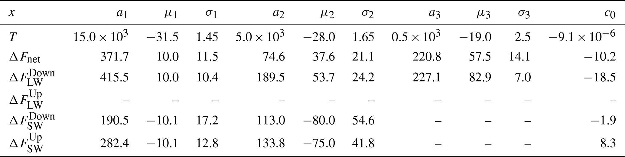
with a_k, μ_k and σ_k being the amplitude, the mean and the standard deviation of the kth Gaussian function and c₀ is a constant. We have used 0, two, or three Gaussians for ΔF components and three Gaussians for T (“0” means that no Gaussian fit was meaningful). Table 2 lists all the fitted parameters (a_k, μ_k, σ_k, and c₀ with k=0 to 3).

Table 2 Gaussian functions fitted to the N(x) function for x=T (^∘C) or ΔF (W m⁻²). Units of a₁, a₂, a₃, and c₀ are count number for T and ΔF, and units of μ₁, μ₂, μ₃, σ₁, σ₂, and σ₃ are ^∘C for T and W m⁻² for ΔF.

In the relationship between x (T or ΔF) and LWP, we have considered x_j (T_j or ΔF_j) to be significant when

$$\begin{array}{}\text{(11)}& \begin{array}{rl}\mathrm{|}{x}_j-{\mathit{\mu }}_k\mathrm{|}\le {\mathit{\sigma }}_k\mathrm{for}& k=\text{1–2}\mathrm{or}\mathrm{3}\left(\mathrm{for}\mathrm{\Delta }F\right)\\ & \mathrm{or}\text{1–3}\left(\mathrm{for}T\right)\end{array}\end{array}$$

and used for this significant point its average value and standard deviation, $\stackrel{\mathrm{‾}}{{\mathrm{LWP}}_j}$ and ${\mathit{\sigma }}_{{\mathrm{LWP}}_j}$, respectively, with j = 1, …, N.

Finally, a logarithmic function of the form

$$\begin{array}{}\text{(12)}& x=\mathit{\alpha }+\mathit{\beta }\ln \left(\stackrel{\mathrm{‾}}{\mathrm{LWP}}\right)\end{array}$$

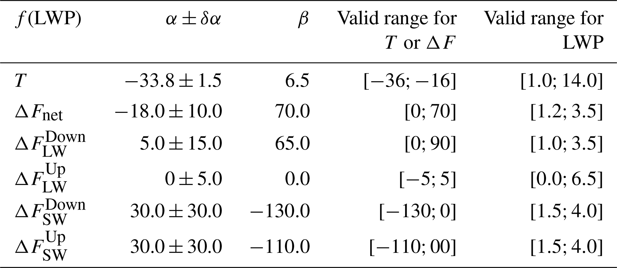
has been fitted onto these significant points where the retrieved constants α and β are shown in Table 3 for x being T, ΔF_net, $\mathrm{\Delta }{F}_{\mathrm{LW}}^{\mathrm{Down}}$, $\mathrm{\Delta }{F}_{\mathrm{LW}}^{\mathrm{Up}}$, $\mathrm{\Delta }{F}_{\mathrm{SW}}^{\mathrm{Down}}$, and $\mathrm{\Delta }{F}_{\mathrm{SW}}^{\mathrm{Up}}$.

Table 3 Coefficients of the relations $f\left(\mathrm{LWP}\right)=\mathit{\alpha }+\mathit{\beta }\ln \left(\mathrm{LWP}\right)$ for the temperature T or cloud radiative forcing (ΔF_net) and the individual components ($\mathrm{\Delta }{F}_{\mathrm{LW}}^{\mathrm{Down}}$, $\mathrm{\Delta }{F}_{\mathrm{LW}}^{\mathrm{Up}}$, $\mathrm{\Delta }{F}_{\mathrm{SW}}^{\mathrm{Down}}$, and $\mathrm{\Delta }{F}_{\mathrm{SW}}^{\mathrm{Up}}$). Units of T and ΔF, as well as of their corresponding “α” values, are ^∘C and W m⁻², respectively; units of β are ^∘C g⁻¹ m² for T and W g⁻¹ for ΔF; and units of LWP are g m⁻². The last column shows the range of LWP values for which the relation is valid. α±δα corresponds to the range of α values where the relationship is valid.

4 Results

4.1 Temperature–liquid water relationship in SLWCs

The relationship between temperature and LWP within SLWCs over the four-summer period at Dome C is presented Fig. 4 left in the form of a probability density (PD) that is the fraction of points within each bin of 0.2 g m⁻² width in LWP and 1.0 ^∘C width in temperature. It clearly shows a net tendency for liquid water to increase with temperature, up to ∼ 14 g m⁻² in LWP and −18 ^∘C in temperature, with two zones having a density as high as ∼ 2 %, at [0.5 g m⁻², −33 ^∘C] and [1.5 g m⁻², −32 ^∘C]. We performed a weighted average of the LWPs within each temperature bin (Fig. 4 centre). Then, we fitted three Gaussian distributions to the count numbers as a function of temperature (Fig. 4 right). If we now only consider temperature bins within 1σ of the centre of the Gaussian distributions, we can fit the following logarithmic relation of the temperature T as a function of LWP within the SLWC (Fig. 4 centre),

$$\begin{array}{}\text{(13)}& T\left(\mathrm{LWP}\right)=-\mathrm{33.8}(\pm \mathrm{1.5})+\mathrm{6.5}\ln \left(\mathrm{LWP}\right),\end{array}$$

for $T\in \left[-\mathrm{36};-\mathrm{16}\right]$ ^∘C and $\mathrm{LWP}\in \left[\mathrm{1.0};\mathrm{14.0}\right]$ g m⁻², with a validity range indicated by the two dashed blue lines (±1.5 ^∘C) in Fig. 4 centre. In other words, based on our study, we have clear evidence that supercooled liquid water content exponentially increases with temperature. Considering the temperature vs. LWP relationship, the two main Gaussian distributions are centred around −28 and −30 ^∘C, corresponding to temperatures usually encountered in Concordia, whilst the third one, far much less intense, is centred around −18 ^∘C, probably the signature of very unusual events occurring in Concordia as the warm, moist events. Episodes of warm, moist intrusions exist above Concordia, originated from mid-latitudes (Ricaud et al., 2017, 2020), and are known as “atmospheric rivers” (Wille et al., 2019). Although they are infrequent, they can provide high values of temperature and LWP.

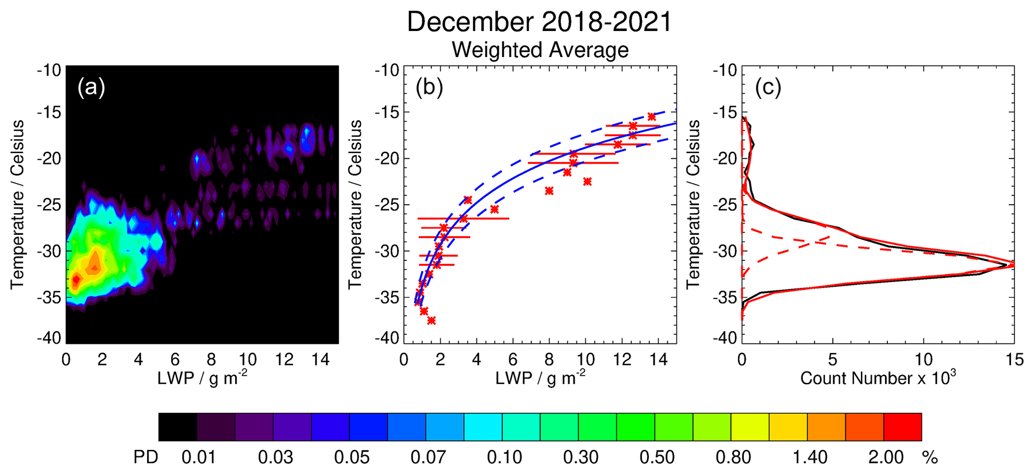
Figure 4 (a) Probability density (PD; %) of the temperature (^∘C) as a function of liquid water path (LWP; g m⁻²) in the SLWCs in December 2018–2021. The probability density is defined in the text. (b) Weighted-average LWP vs. temperature (red asterisks) with a fitted logarithmic function (solid blue) encompassing the significant points (within the two dashed blue lines). Horizontal bars represent 1σ variability in LWP per 1 ^∘C wide bin. (c) Temperature as a function of count number per 1 ^∘C wide bin (solid black line) fitted with three Gaussian functions (dashed red curves). The sum of the three Gaussian functions is represented by a solid red line.

4.2 Radiative forcing–liquid water relationship in SLWC conditions

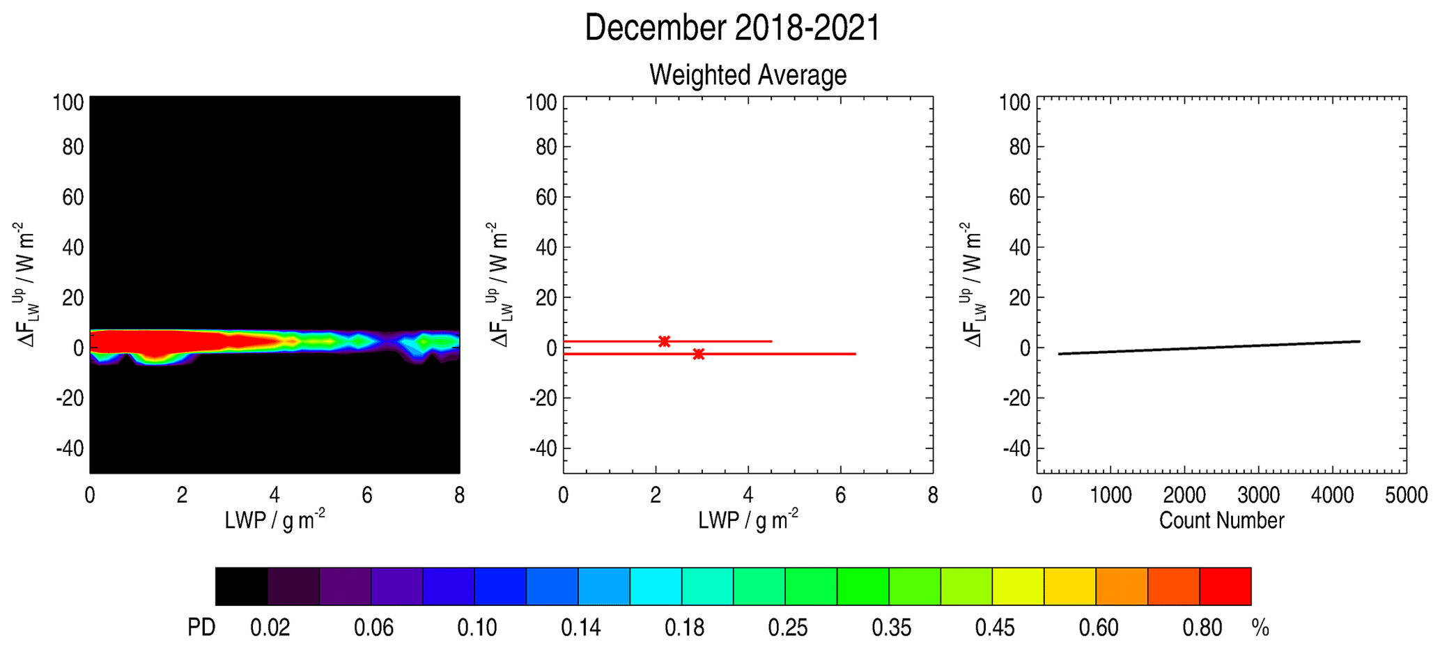
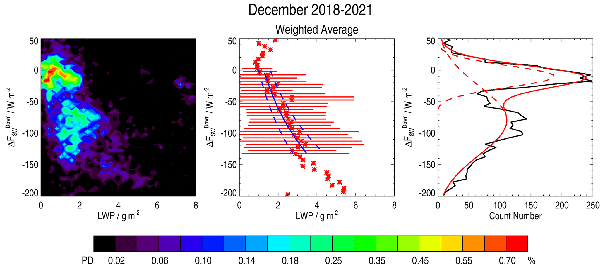
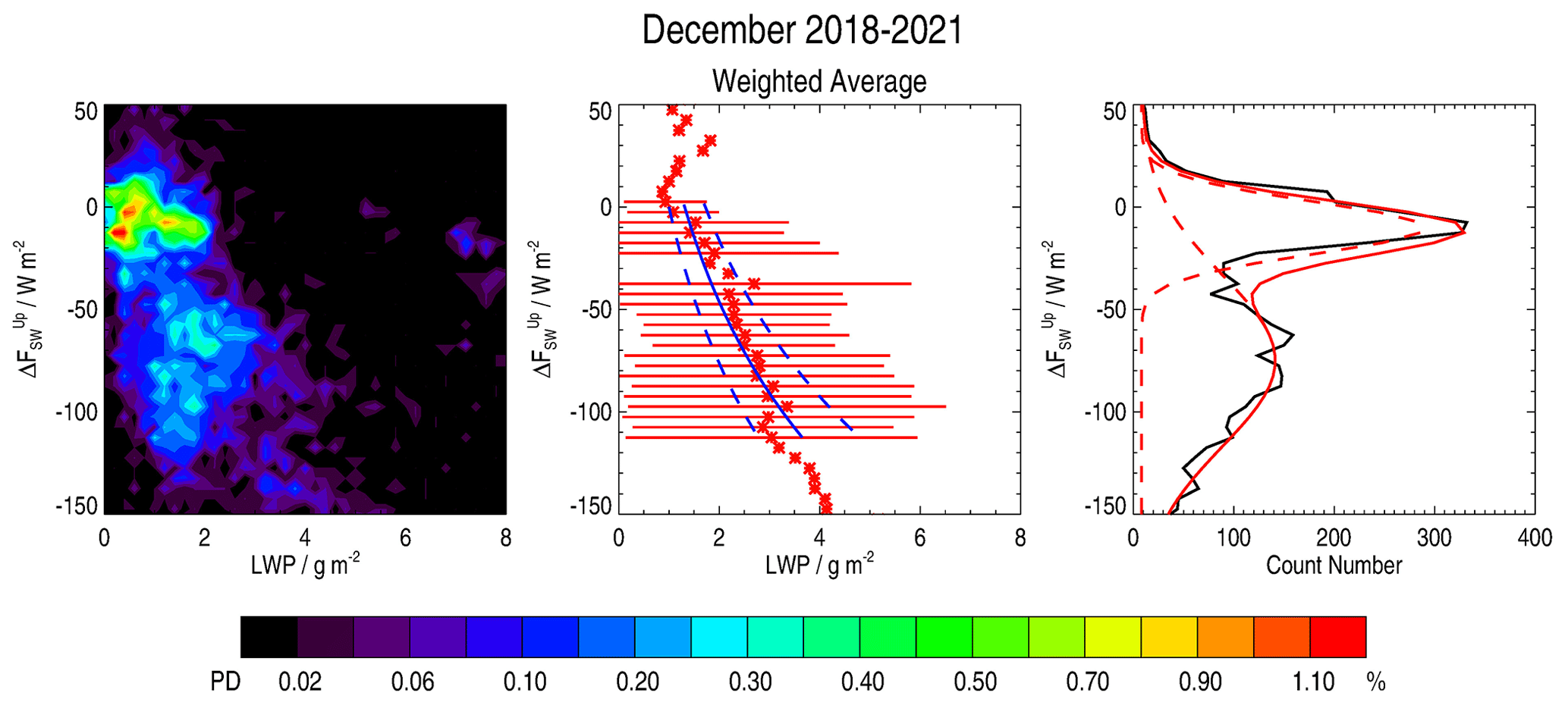
Although the amount of LWP is very low (<20 g m⁻²) at Dome C compared to what can be measured and modelled (Lemus et al., 1997) in the Arctic (50 to 75 g m⁻²) and at middle/tropical latitudes (100 to 150 g m⁻²), we intended to estimate its impact on the cloud radiative forcing at Dome C. In Figs. 5 to 9, the left panel presents the PDs of the cloud radiative forcing ΔF_net as a function of the LWP and for the individual components that contribute to the cloud radiative forcing: $\mathrm{\Delta }{F}_{\mathrm{LW}}^{\mathrm{Down}}$, $\mathrm{\Delta }{F}_{\mathrm{LW}}^{\mathrm{Up}}$, $\mathrm{\Delta }{F}_{\mathrm{SW}}^{\mathrm{Down}}$, and $\mathrm{\Delta }{F}_{\mathrm{SW}}^{\mathrm{Up}}$, respectively. The central panel shows, for the same parameters, the corresponding weighted average LWP within 5 W m⁻² wide bins of ΔF, whereas the right panel shows the corresponding count number within 5 W m⁻² wide bins fitted by 2 or 3 Gaussian distributions (or no Gaussian distribution when it becomes impossible).

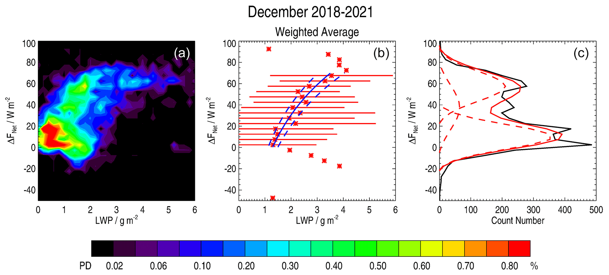
Figure 5 (a) Probability density (PD; %) of the cloud radiative forcing (ΔF_net, W m⁻²) as a function of liquid water path (LWP; g m⁻²) in the SLWCs in December 2018–2021. The probability density is defined in the text. (b) Weighted-average LWP vs. ΔF_net with a fitted logarithmic function (solid blue) encompassing the significant points (within the two dashed blue lines). Horizontal bars represent 1σ variability in LWP per 5 W m⁻² wide bin. (c) ΔF_net as a function of count number per 5 W m⁻² wide bin (solid black line) fitted with 3 Gaussian functions (dashed red curves). The sum of the 3 Gaussian functions is represented by a solid red line.

Figure 6 As in Fig. 5 but for $\mathrm{\Delta }{F}_{\mathrm{LW}}^{\mathrm{Down}}$.

Figure 7 As in Fig. 5 but for $\mathrm{\Delta }{F}_{\mathrm{LW}}^{\mathrm{Up}}$.

Figure 8 As in Fig. 5 but for $\mathrm{\Delta }{F}_{\mathrm{SW}}^{\mathrm{Down}}$.

Figure 9 As in Fig. 5 but for $\mathrm{\Delta }{F}_{\mathrm{SW}}^{\mathrm{Up}}$.

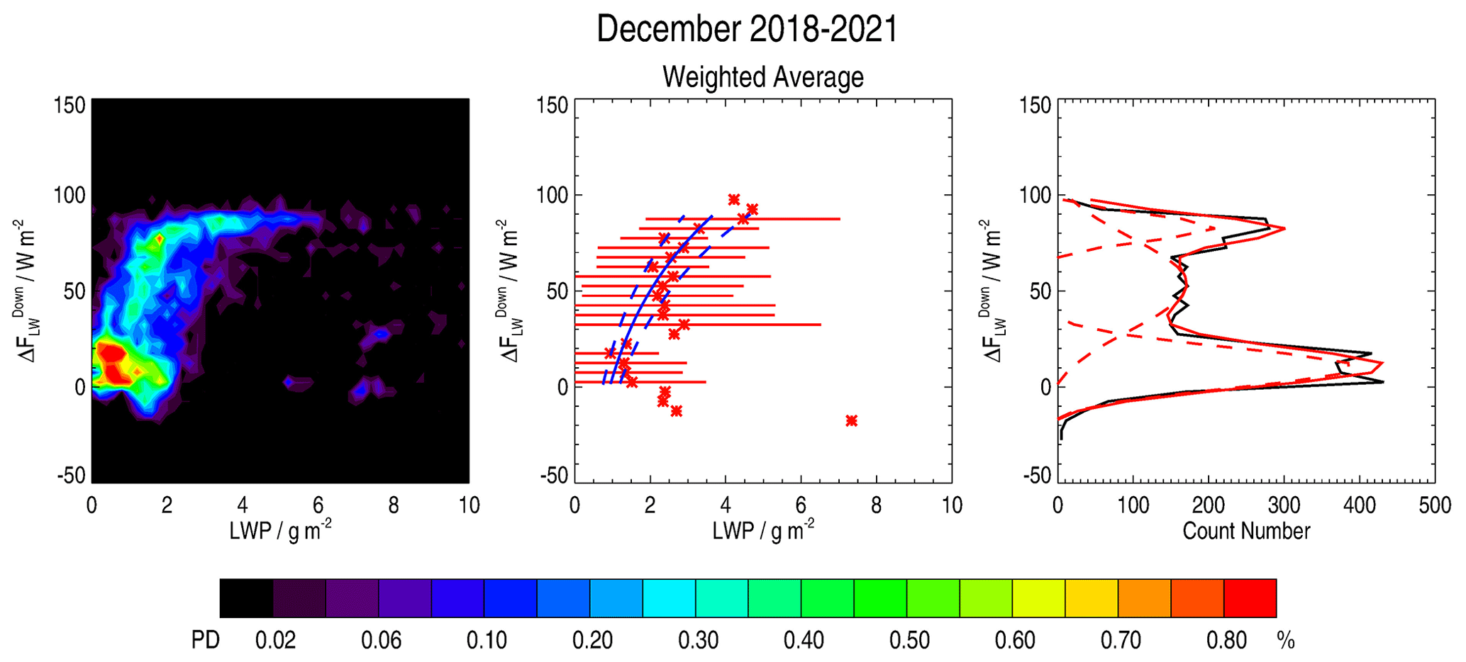
Based on our analysis, the relationship between ΔF_net (W m⁻²) and the LWP (g m⁻²) has been estimated as

$$\begin{array}{}\text{(14)}& \mathrm{\Delta }{F}_{\mathrm{net}}\left(\mathrm{LWP}\right)=-\mathrm{18.0}(\pm \mathrm{10.0})+\mathrm{70.0}\ln \left(\mathrm{LWP}\right),\end{array}$$

for $\mathrm{\Delta }{F}_{\mathrm{net}}\in \left[\mathrm{0};\mathrm{70}\right]$ W m⁻² and $\mathrm{LWP}\in \left[\mathrm{1.2};\mathrm{3.0}\right]$ g m⁻², with a validity range indicated by the two dashed blue lines (±10.0 W m⁻²) in Fig. 5 centre. Thus, for LWP greater than 1.2 g m⁻², our study clearly shows that the cloud radiative forcing induced by the presence of SLWCs above Concordia is positive and can reach 70 W m⁻² for an LWP of 3.0 g m⁻².

The splitting of the cloud radiative forcing between each of its four components can be evaluated from their individual relationships with the LWP. These relations are gathered in Table 3, established from the plots presented in Figs. 5 to 9. They are of the same form as for cloud radiative forcing, i.e. a logarithmic dependence on LWP. Table 3 presents the coefficients α and β of the logarithmic function $f\left(\mathrm{LWP}\right)=\mathit{\alpha }+\mathit{\beta }\ln \left(\mathrm{LWP}\right)$ for the temperature T or the radiation components ΔF, together with the valid range of these relations for T, ΔF and LWP. For the values presented in Table 3, our study clearly shows that SLWCs have a positive impact on $\mathrm{\Delta }{F}_{\mathrm{LW}}^{\mathrm{Down}}$ increasing from 0 to 90 W m⁻² for LWP ranging from 1.0 to 3.5 g m⁻², a negative impact on $\mathrm{\Delta }{F}_{\mathrm{SW}}^{\mathrm{Down}}$ and $\mathrm{\Delta }{F}_{\mathrm{SW}}^{\mathrm{Up}}$ decreasing from 0 to −130 and −110 W m⁻², respectively, for LWP ranging from 1.5 to 4.0 g m⁻², and a negligible impact (±5 W m⁻²) on $\mathrm{\Delta }{F}_{\mathrm{LW}}^{\mathrm{Up}}$ for LWP ranging from 0 to 6.5 g m⁻². Considering the absolute values of the ΔF vs. LWP relationship (keeping aside $\mathrm{\Delta }{F}_{\mathrm{LW}}^{\mathrm{Up}}$), we systematically have the most intense Gaussian distributions centred at ∼ 10 W m⁻² and the other ones centred at ∼ 55 and ∼ 80 W m⁻².

To summarize, our study showed that the major impact of SLWCs on net surface irradiance is an increase in the downward longwave component (0 to 80 W m⁻²), whereas it has a marginal impact on upward longwave component since this parameter is mainly dependent on T_s which results from various meteorological forcings. In the presence of SLWC, the attenuation of shortwave incoming irradiance (which can overpass 100 W m⁻²) is almost compensated for by the upward shortwave irradiance because of high values of surface albedo.

We can also estimate the sensitivity of the longwave component to temperature and humidity by considering the values of the equivalent atmospheric emissivity ε_a used in the Eqs. (4)–(7). On the one side, the values of IWV observed at Dome C are very low even in summer; typical summertime values are between 0.8 and 1.2 kg m⁻² (Ricaud et al., 2020). This corresponds to values of ε_a between 0.950 and 0.985, i.e. a relative variation of the order of 3.6 %. On the other side, a variation ΔT in the screen-level air (surface) temperature T_a (T_s) has a relative impact on the downwelling (upwelling) longwave irradiance of the order of $\mathrm{4}\mathrm{\Delta }T/T_{\mathrm{s}}$), which amounts to around 1.6 % per degree of ΔT. Given that observations of surface and screen-level air temperatures reveal variations of several degrees, both in their diurnal cycle and from one day to another, we can conclude that the impact of temperature on longwave irradiance variations is larger than that of IWV.

5 Discussion

5.1 Relation with critical temperature

Our study shows that, above Concordia, there is an exponential dependence of LWP on both temperature and cloud radiative forcing; that is to say supercooled liquid water exponentially increases with temperature in the range −36 to −16 ^∘C. This is in agreement with the outputs from a simple model for thermodynamic properties of water from sub-zero temperatures up to +100 ^∘C (Sippola and Taskinen, 2018). The model shows that the density ρ (g cm⁻³) of liquid water exponentially increases with temperature from −34 to 0 ^∘C through the following relationship:

$$\begin{array}{}\text{(15)}& \mathit{\rho }={\mathit{\rho }}_{\mathrm{0}}\exp \left\{-T_{\mathrm{c}}(A+B{\mathit{\epsilon }}_{\mathrm{0}}+\mathrm{2}C{\mathit{\epsilon }}_{\mathrm{0}}^{\mathrm{1}/\mathrm{2}})\right\},\end{array}$$

where ρ₀=1.007853 g cm⁻³, $A=\mathrm{3.9744}\times {\mathrm{10}}^{-\mathrm{4}}$ K⁻¹, $B=\mathrm{1.6785}\times {\mathrm{10}}^{-\mathrm{3}}$ K⁻¹, and $C=-\mathrm{7.8165}\times {\mathrm{10}}^{-\mathrm{4}}$ K⁻¹. T_c is the critical temperature (K), and ε₀ (unitless) is defined as

$$\begin{array}{}\text{(16)}& {\mathit{\epsilon }}_{\mathrm{0}}={\displaystyle \frac{T}{T_{\mathrm{c}}}}-\mathrm{1},\end{array}$$

where T is temperature in kelvin. In thermodynamics, a critical point is the end point of a phase equilibrium curve. In our study, the liquid–ice boundary terminates at some critical temperature T_c. T_c is about 224.8 K if water is pure and free of nucleation nuclei. Sippola and Taskinen (2018) reviewed a value of T_c ∼ 227–228 K (approx. −45 ^∘C) in the literature. This is also in agreement with the results from our study showing that, above Concordia, we could not observe SLWCs at temperatures less than −36 ^∘C, consistent with the fact that the threshold temperature to get SLWCs should be around −39 ^∘C (see the discussions on errors in Sect. 5.3).

5.2 Modelling SLWC

Previous studies have already underlined the difficulty of modelling the SLWC together with its impact on surface radiations. Modelling SLWCs over Antarctica is challenging because (1) operational observations are scarce since the majority of meteorological radiosondes are released from ground stations located on the coast, and very few of them are maintained all year long, and satellite observations are limited to 60^∘ S in geostationary orbit, whilst, in a polar orbit, the number of available orbits does not exceed 15 d⁻¹, and (2) the model should provide a partition function favouring liquid water at the expense of ice for temperatures between −36 and 0 ^∘C in order to calculate realistic SLW contents. Differences of 20 to 50 W m⁻² in the net surface irradiance were found in the Arpege model (Pailleux et al., 2015) between clouds made of ice or liquid water during the summer 2018–2019 (Ricaud et al., 2020), differences that are very consistent with the results obtained in the present study. Although SLWCs are less present over the Antarctic Plateau than over the coastal region, their radiative impact is not negligible and should be taken into account with great care in order to estimate the radiative budget of the Antarctic continent on the one hand and, on the other hand, over the entire Earth.

5.3 Errors

Measurements of temperature, LWP, depolarization signal, and surface irradiances F are altered by random and systematic errors that may affect the relationships we have obtained between LWP and either temperature or cloud radiative forcing ΔF_net and its individual components. The temperature measured by HAMSTRAD below 1 km has been evaluated against radiosonde coincident observations from 2009 to 2014 (Ricaud et al., 2015), and the resulting bias is 0 to 2 ^∘C below 100 m and between −2 and 0 ^∘C between 100 and 1000 m. SLWCs are usually located around 400–600 m a.g.l. where the cold bias can be estimated to be about −1.0 ^∘C. The one-sigma (1σ) rms temperature error over a 7 min integration time is 0.25 ^∘C in the PBL and 0.5 ^∘C in the free troposphere (Ricaud et al., 2015). As a consequence, given the number of points used in the statistical analysis (>1000), the random error on the weighted-average temperature is negligible (<0.02 ^∘C). The LWP random and systematic errors are difficult to evaluate since there is no coincident external data to compare with. Nevertheless, the 1σ rms error over a 7 min integration time can be estimated to be 0.25 g m⁻², giving a random error on the weighted average LWP of less than 0.08 g m⁻². Based on clear-sky observations, the positive bias can be estimated to be of the order of 0.4 g m⁻². Theoretically, SLW should not exist at temperatures less than −39 ^∘C, although it has been observed in recent laboratory measurements down to −42.55 ^∘C (Goy et al., 2018). Using Eq. (13) with an LWP bias of 0.4 g m⁻² gives a temperature of −39.8 ^∘C (∼ 0.8 ^∘C lower than the theoretical limit of −39 ^∘C), so the biases estimated for temperature and LWP are very consistent with theory.

The estimation of systematic and random errors on lidar backscattering and depolarization signals and their impact on the attribution/selection of SLWC is not trivial. But the most important point is to evaluate whether the observed cloud is constituted of purely liquid or mixed-phase water. Even considering the backscatter intensity only, we could not exclude that ice particles could have been present in the SLWC events investigated in 2018 (Ricaud et al., 2020). Therefore, in the present analysis, although we gave great attention to diagnosing ice in the lidar cloud observations, we cannot totally exclude ice particles; thus mixed-phase parcels were actually present when we labelled the observed cloud as SLWCs.

The four instruments providing $F_{\mathrm{LW}}^{\mathrm{Down}}$, $F_{\mathrm{LW}}^{\mathrm{Up}}$, $F_{\mathrm{SW}}^{\mathrm{Down}}$, and $F_{\mathrm{SW}}^{\mathrm{Up}}$ follow the rules of acquisition, quality check, and quality control of the BSRN (Driemel et al., 2018). These data are often considered as a reference against which products based on satellite observations and radiative transfer models (such as CERES) are validated (Kratz et al., 2020). In polar regions (Lanconelli et al., 2011), $F_{\mathrm{SW}}^{\mathrm{Down}}$ and $F_{\mathrm{SW}}^{\mathrm{Up}}$ are expected to be affected by random errors up to ±20 W m⁻², while $F_{\mathrm{LW}}^{\mathrm{Down}}$ is expected to be affected by random errors not greater than ±10 W m⁻² (Ohmura et al., 1998). As a consequence, given the large number of observations used per 5 W m⁻² wide bins (1000–3000), the random error on the weighted-average F is negligible (0.3 to 0.7 W m⁻²), whatever the radiations considered, LW and SW.

Finally, another source of error comes from (1) the geometry of observation and (2) the discontinuous SLWC layer. Firstly, lidar is almost zenith pointing, and HAMSTRAD conducts a scan in the east direction (from 10^∘ elevation to zenith), whilst the BSRN radiometers detect the radiation in a 2π-steradian field of view (3D configuration). That is to say, in our analysis, the whole sky contributes to the radiation, whilst only the cloud at zenith (1D configuration) and in the east direction (2D configuration) is observed by the lidar and HAMSTRAD, respectively. Secondly, SLWCs cannot be considered uniform, covering the whole sky (see, for example, broken cloud fields in Fig. 2).

5.4 Other clouds

Although the method we have developed to select the SLWCs has been validated using the amount of LWP and, in another study, using space-borne observations (Ricaud et al., 2020), we cannot rule out that, associated with the SLW droplets, there are also ice particles; that is clouds are constituted of a mixture of liquid and solid water. Statistics of ice and mixed-phase clouds over the Antarctic Plateau have been performed by Cossich et al. (2021), revealing mean annual occurrences of 72.3 %, 24.9 %, and 2.7 % for clear sky, ice clouds, and mixed-phase clouds, respectively. Generally, mixed-phase clouds are a superposition of a lower layer made of liquid water and an upper layer made of solid water (see Fig. 12.3 from Lamb and Verlinde, 2011). These mixed-layer clouds do not significantly modify the relationship between temperature and LWP because (1) SLW observations from HAMSTRAD are only sensitive to water in liquid phase, and (2) temperature from HAMSTRAD is selected at times and vertical heights where the lidar depolarization signal is very low (<5 %). Although we have verified that pure ice clouds were not selected by our method, we cannot differentiate mixed-phase clouds from purely SLWCs.

Furthermore, we already have noticed that SLWCs developed at the top of the PBL (Ricaud et al., 2020) in the “entrainment zone” and stayed in the “capping inversion zone”, following the terminology of Stull (1988), at a height, ranging from 100 to 1000 m a.g.l. Nevertheless, at 00:00–06:00 LT when the sun is at low elevation above the horizon (24 h polar day), the PBL may collapse down to a very low height ranging 20–50 m. In this configuration, it is hard to differentiate from lidar observations between a SLWC and a fog episode, although the lidar can measure depolarization (but not backscatter) down to approximately 10–30 m a.g.l. (Fig. S3 in Chen et al., 2017), so that we can distinguish liquid and frozen clouds very close to the ground.

Finally, we cannot rule out that, above the SLWCs that are actually observed by both lidar and HAMSTRAD, other clouds might be present, for example, cirrus clouds constituted of ice crystals. These middle–upper-tropospheric clouds cannot be detected by HAMSTRAD (no sensitivity to ice crystals). In the presence of SLWCs either low in altitude or optically thick, the lidar backscatter signal is decreased in order to avoid saturation, and the signal from upper layers is thus almost cancelled. These mid-latitude–high-altitude clouds are sensed by the BSRN instruments, and surface irradiance can be affected in this configuration. Based on the presence of cirrus clouds before or after the SLWCs (and sometimes during the SLWCs if optically thin), we can estimate the number of days when SLWCs and cirrus clouds are simultaneously present to cover less than 10 % of our period of interest.

5.5 Sastrugi effect on the surface albedo

Sastrugi are features formed by erosion of snow by wind. They are found in polar regions and in snowy, wind-swept areas of temperate regions, such as frozen lakes or mountain ridges. Sastrugi are distinguished by upwind-facing points, resembling anvils, which move downwind as the surface erodes.

Figure 10 shows the BSRN surface albedo averaged over the 5 cloud-free days (2 and 19 December 2018; 3, 17, and 26 December 2021), showing a clear diurnal signal with a maximum of 0.85 from 10:00 to 14:00 UTC (from 18:00 to 22:00 LT) and a minimum of 0.70 from 19:00 to 23:00 UTC (from 03:00 to 07:00 LT). The large diurnal signal present in the observed surface albedo is likely the signature of (1) the sastrugi orientation and also (2) the sun zenith angle which impacts on the surface albedo, even with a flat snow surface (Gardner and Sharp, 2010). Note that the surface albedo of snow under cloudy conditions may differ from the surface albedo under cloud-free conditions (e.g., Gardner and Sharp, 2010; Stapf et al., 2020). The BSRN $F_{\mathrm{SW}}^{\mathrm{Up}}$ sensor has a circular footprint. For a sensor installed at a height h above the ground, 90 % of the signal comes from an area at the surface closer than 3.1 h (Kassianov et al., 2014). Since at Dome C the instrument is installed at a height of 2–3 m, the surface albedo is determined by the surface elements in the immediate vicinity (a few metres) of the sensor.

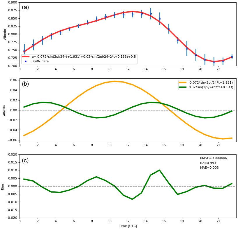
Figure 10 (a) Hourly time evolution (UTC, hour) of the mean surface albedo observed by the BSRN instruments and the associated standard deviation (blue star and vertical bar, respectively) for the five cloud-free periods under consideration in our analysis, together with the fitted trigonometric function based on two sine functions (red line). (b) The two sine functions fitting the hourly time evolution of the BSRN mean surface albedo. (c) Hourly time evolution (UTC, hour) of the albedo residuals (BSRN fit, green line) and corresponding values of associated root mean square error (RMSE), coefficient of determination (R²), and mean absolute error (MAE).

We have fitted the averaged cloud-free BSRN surface albedo with the sum of two sine functions, imposing periods of 24 and 12 h (Fig. 10) together with the residuals between the averaged surface albedo and the fitted function. We can state that the sastrugi effect on the observed cloud-free surface albedo at Concordia is successfully fitted by two sine functions of 24 and 12 h periods to within 0.003 mean absolute error, with a coefficient of determination R² equal to 0.993 and a root mean square error of 0.0004.

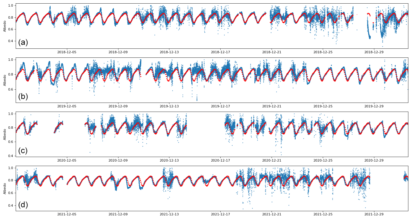
Figure 11 (a–d) Hourly time evolution (UTC) of the surface albedo observed by the BSRN instruments (blue) and using the fit based on two sine functions (red) for the whole BSRN dataset covering the month of December in 2018, 2019, 2020, and 2021.

Moreover, we have considered all the BSRN observations in the month of December in the years 2018, 2019, 2020, and 2021 to calculate the surface albedo (Fig. 11), and we have superimposed the fitted trigonometric function as described in Fig. 10. The presence of clouds is highlighted well by observations that depart from the fitted function, whilst, during periods of clear-sky conditions, BSRN surface albedos coincide well with the fitted function. To conclude, the surface albedo at Concordia should be treated considering the sastrugi effect.

5.6 Maximum SLWC radiative forcing over Antarctica

Based on 2007–2010 reanalyses, observations, and climate models (Lenaerts et al., 2017), LWP over Antarctica is on average less than 10 g m⁻², with slightly larger values in summer than in winter by 2 to 5 g m⁻². Over West Antarctica, LWPs are larger (20 to 40 g m⁻²) than over East Antarctica (0 to 10 g m⁻²). As a consequence, LWPs observed at Concordia are consistent with values observed over the eastern Antarctic Plateau, which are a factor of 2 to 4 smaller than those observed over the western continent. Based on our results and on the observed cloud fraction (η_CF) of SLWCs over Antarctica for different seasons (Listowski et al., 2019), we can estimate the maximum SLWC radiative forcing at the scale of the Antarctic continent ($\mathrm{\Delta }{F}_{\text{Net-Ant}}^{max}$) from the maximum of ΔF_net ($\mathrm{\Delta }{F}_{\mathrm{Net}}^{\max }=\mathrm{70}$ W m⁻²) computed in our study:

$$\begin{array}{}\text{(17)}& \mathrm{\Delta }{F}_{\text{Net-Ant}}^{\max }={\mathit{\eta }}_{\mathrm{CF}}\times \mathrm{\Delta }{F}_{\mathrm{Net}}^{\max }.\end{array}$$

Equation (17) assumes a linear dependence between cloud fraction and cloud radiative forcing, although, in nature, there could be three-dimensional radiation effects. In summer, η_CF varies from 5 % in East Antarctica to 40 % in West Antarctica, whilst, in winter, it varies from 0 % in East Antarctica to 20 % in West Antarctica (Listowski et al., 2019). In December, if we consider η_CF for SLW-containing cloud (that is to say both mixed-phase cloud and unglaciated SLW cloud consistent with our study), we find for a lower-level altitude cut-off of 0, 500, and 1000 m (Fig. B1 in Listowski et al., 2019) a maximum SLWC radiative forcing $\mathrm{\Delta }{F}_{\text{Net-Ant}}^{\max }$ over Antarctica of about 12, 10 and 7 W m⁻², respectively. We now separate the eastern elevated Antarctic Plateau from West Antarctica (Fig. 5 in Listowski et al., 2019) for the four seasons. Over East Antarctica, we find that $\mathrm{\Delta }{F}_{\text{Net-Ant}}^{\max }=\mathrm{0.7}$ to 7.0 W m⁻² in December–January–February (DJF) and 0 to 3.5 W m⁻² for the remaining seasons. Over West Antarctica, the maximum radiative impact is much more intense because of higher temperatures and lower elevations compared to the eastern Antarctic Plateau: $\mathrm{\Delta }{F}_{\text{Net-Ant}}^{\max }=\mathrm{17.5}$ to 40.0 W m⁻² in DJF (40 W m⁻² over the Antarctica Peninsula), 10.5 to 28.0 W m⁻² in March–April–May, 3.5 to 14.0 W m⁻² in June–July–August, and 7.0 to 17.5 W m⁻² in September–October–November. To summarize, the maximum SLWC radiative forcing over West Antarctica (0 to 40 W m⁻²) is estimated to be 3 to 5 times larger compared to the one over the eastern Antarctic Plateau (0 to 7 W m⁻²), maximizing during the summer season.

6 Conclusions

Combining the observations of temperature, water vapour and liquid water path from a ground-based microwave radiometer; backscattering and depolarization from a ground-based lidar; screen-level air temperature; and surface radiations at long and short wavelengths, our analysis has been able to evaluate the presence of supercooled liquid water clouds over the Dome C station in summer. Focusing on the month of December in 2018–2021, we established that in SLWCs, temperature logarithmically increases from −36.0 to −16.0 ^∘C when LWP increases from 1.0 to 14.0 g m⁻². We have also evaluated that SLWCs have a positive cloud radiative forcing, which logarithmically increases from 0.0 to 70.0 W m⁻² when LWP increases from 1.2 to 3.5 g m⁻². Our study clearly shows that SLWCs have a positive impact on $\mathrm{\Delta }{F}_{\mathrm{LW}}^{\mathrm{Down}}$ increasing from 0 to 90 W m⁻² for LWP ranging from 1.0 to 3.5 g m⁻²; a negligible impact (±5 W m⁻²) on $\mathrm{\Delta }{F}_{\mathrm{LW}}^{\mathrm{Up}}$ for LWP ranging from 0 to 6.5 g m⁻²; and a negative (but quite offsetting) impact on each of the two terms $\mathrm{\Delta }{F}_{\mathrm{SW}}^{\mathrm{Down}}$ and $\mathrm{\Delta }{F}_{\mathrm{SW}}^{\mathrm{Up}}$, which decrease from 0 to −130 and −110 W m⁻², respectively, for LWP ranging from 1.5 to 4.0 g m⁻². This means that the SLWC radiative forcing is mainly driven by the downward surface irradiance since the attenuation of shortwave incoming irradiance is almost compensated for by the upward shortwave irradiance because of high values of surface albedo.

Finally, extrapolating our results of the SLWC radiative forcing from the Dome C station to the Antarctic continent shows that the maximum SLWC radiative forcing is not greater than 7.0 W m⁻² over the eastern Antarctic Plateau but 2 to 3 times larger (up to 40 W m⁻²) over West Antarctica, maximizing in the summer season and over the Antarctic Peninsula. This stresses the importance of accurately modelling SLWCs when calculating the Earth energy budget to adequately forecast the Earth climate evolution, especially since the climate is rapidly changing in Antarctica, as illustrated by the surface temperature record of −12 ^∘C recently observed in March 2022 at the Concordia station and largely publicized worldwide (see, for example, https://www.9news.com.au/world/antarctica-heatwave-extreme-warm-weather-recorded-concordia-research-station/3364dd91-2051-4df5-8cfc-5f2819058604, last access: 12 January 2024).