the Creative Commons Attribution 4.0 License.
the Creative Commons Attribution 4.0 License.
 | 27 May 2024
Combined assimilation of NOAA surface and MIPAS satellite observations to constrain the global budget of carbonyl sulfide
Linda M. J. Kooijmans
Norbert Glatthor
Stephen A. Montzka
Marc von Hobe
Thomas Röckmann
Carbonyl sulfide (COS), a trace gas in our atmosphere that leads to the formation of aerosols in the stratosphere, is largely taken up by terrestrial ecosystems. Quantifying the biosphere uptake of COS could provide a useful quantity to estimate gross primary productivity (GPP). Some COS sources and sinks still contain large uncertainties, and several top-down estimates of the COS budget point to an underestimation of sources, especially in the tropics. We extended the inverse model TM5-4DVAR to assimilate Michelson Interferometer for Passive Atmospheric Sounding (MIPAS) satellite data, in addition to National Oceanic and Atmospheric Administration (NOAA) surface data as used in a previous study. To resolve possible discrepancies among the two observational data sets, a bias correction scheme is necessary and implemented. A set of inversions is presented that explores the influence of the different measurement streams and the settings of the prior fluxes. To evaluate the performance of the inverse system, the HIAPER Pole-to-Pole Observations (HIPPO) aircraft observations and NOAA airborne profiles are used. All inversions reduce the COS biosphere uptake from a prior value of 1053 GgS a−1 to much smaller values, depending on the inversion settings. These large adjustments of the biosphere uptake often turn parts of Amazonia into a COS source. Only inversions that exclusively use MIPAS observations, or strongly reduce the prior errors on the biosphere flux, maintain the Amazon as a COS sink. Inclusion of MIPAS data in the inversion leads to a better separation of land and ocean fluxes. Over the Amazon, these inversions reduce the biosphere uptake from roughly 300 to 100 GgS a−1, indicating a strongly overestimated prior uptake in this region. Although a recent study also reported reduced COS uptake over the Amazon, we emphasise that a careful construction of prior fluxes and their associated errors remains important. For instance, an inversion that gives large freedom to adjust the anthropogenic and ocean fluxes of CS2, an important COS precursor, also closes the budget satisfactorily with much smaller adjustments to the biosphere. We achieved better characterisation of biosphere prior and uncertainty, better characterisation of combined ocean and land fluxes, and better constraint of both by combining surface and satellite observations. We recommend more COS observations to characterise biosphere and ocean fluxes, especially over the data-poor tropics.
- Article
(9528 KB) - Full-text XML
-
Supplement
(6926 KB) - BibTeX
- EndNote


Understanding sources and sinks of greenhouse gases is a scientific challenge (Friedlingstein et al., 2020, 2022a, b). One important climate-related process is the carbon uptake by terrestrial ecosystems, named gross primary productivity (GPP). However, accurate estimation of GPP is difficult, since the measured net flux of carbon at ecosystem level is determined by both GPP and ecosystem respiration. In the recent decade, GPP proxy methods have been developed with the aim to improve GPP estimates (Campbell et al., 2008; Wingate et al., 2010; Berry et al., 2013; Commane et al., 2015; Koren, 2021).
Carbonyl sulfide (COS), a low-abundant and long-lived trace gas with an average mixing ratio of about 500 pmol mol−1 in the Earth's atmosphere (Montzka et al., 2007; Kremser et al., 2016), is biochemically coupled with CO2 (Stimler et al., 2010; Campbell et al., 2008; Berry et al., 2013) and is a major contributor to stratospheric sulfur aerosols (Crutzen, 1976; Turco et al., 1980; Brühl et al., 2012). The concentration of COS remains relatively constant and shows small inter-annual variability, implying that the sources and sinks of COS are roughly balanced (Montzka et al., 2007). A recent study based on vertical column measurements in the Network for the Detection of Atmospheric Composition Change (NDACC) (Hannigan et al., 2022) reported a slightly increasing tropospheric trend in free tropospheric COS ranging from ∼0.0 to 1.55±0.30 % a−1 in 2002–2016 that appears correlated with estimates of anthropogenic emissions (Hannigan et al., 2022). In the period 2016–2020, all NDACC stations showed a free tropospheric decline in COS. Besides direct emissions of COS, carbon disulfide (CS2) and dimethyl sulfide (DMS) are species that potentially account for substantial chemical production of COS in the troposphere (Chin and Davis, 1993; Watts, 2000; Kettle et al., 2002; Ma et al., 2021; Jernigan et al., 2022).
COS is absorbed by terrestrial vegetation through photosynthesis sharing a similar pathway to CO2, but it is not emitted from vegetation through respiration, which makes COS a promising diagnostic tracer to improve estimates of GPP globally (Wohlfahrt et al., 2012; Berry et al., 2013; Campbell et al., 2017; Whelan et al., 2018). Recently, COS observations have been used to estimate regional GPP over arctic North America and boreal regions (Hu et al., 2021) and over Amazonia (Stinecipher et al., 2022) and to detect city-level signals from the urban biosphere (Villalba et al., 2021). Besides, isotopologue measurement and modelling studies are being used to differentiate signals from various sources and sinks (Hattori et al., 2020; Davidson et al., 2021; Baartman et al., 2021; Nagori et al., 2022). In parallel, COS flux measurements combined with land surface models improve our understanding of the interaction of COS with plants and soils (Kooijmans et al., 2017, 2019; Spielmann et al., 2019; Kooijmans et al., 2021; Maignan et al., 2021; Wu et al., 2015; Ogée et al., 2016; Abadie et al., 2022). Inverse modelling to better constrain the global COS budget is also readily progressing (Suntharalingam et al., 2008; Berry et al., 2013; Wang et al., 2016; Kuai et al., 2015; Ma et al., 2021; Remaud et al., 2022; Stinecipher et al., 2022).
The COS abundance and variability in the atmosphere is determined by multiple sources and sinks. Anthropogenic, oceanic and biomass burning emissions are the major sources of COS. The inventories of COS and CS2 anthropogenic emissions are in the range of 223–586 GgS a−1 (Campbell et al., 2015; Zumkehr et al., 2018). Specifically for China, anthropogenic emission estimates were reported as 174 GgS a−1 in 2015 (Yan et al., 2019), of which 31 GgS a−1 was from domestic coal combustion (Du et al., 2016). Global emissions from oceans of 600–800 GgS a−1 would be required to balance the global COS budget (Berry et al., 2013; Glatthor et al., 2015; Kuai et al., 2015), but a mechanistic ocean box model and COS seawater measurements suggest that direct COS oceanic emissions are unlikely to fully account for the large missing source (Lennartz et al., 2017, 2021, 2020). Biomass burning emissions of COS, estimated as 60±37 GgS a−1 by Stinecipher et al. (2019) without accounting for biofuel, is unlikely to account for the missing source as well. More recently, a new chemical product of DMS oxidation known as hydroperoxymethyl thioformate (HPMTF) was discovered and may play a role in accounting for the missing sources of COS in the troposphere (Wu et al., 2015; Veres et al., 2020; Fung et al., 2022; Jernigan et al., 2022).
On the uptake part of the budget, the largest sink of COS is uptake by terrestrial vegetation and soils, with estimates ranging from −500 to −1200 GgS a−1 (Campbell et al., 2008; Suntharalingam et al., 2008; Berry et al., 2013; Remaud et al., 2022). Kooijmans et al. (2021) recently updated the COS biosphere uptake based on the Simple Biosphere model (SiB4), and the estimate is from −922 to −753 GgS a−1, by considering the linear dependency of the flux on the atmospheric COS mole fraction and COS soil production. This estimate is also in line with inverse modelling studies, which report fluxes that range from −1053 to −862 GgS a−1 (Ma et al., 2021). The uncertainty in COS biosphere uptake introduced by the soil flux was large (Whelan et al., 2013, 2016, 2018), and Abadie et al. (2022) reported a global net soil sink of only −30 GgS a−1 over the 2009–2016 period. Finally, chemical loss by OH-induced tropospheric oxidation and stratospheric photolysis contribute respectively about −100 GgS a−1 (Kettle et al., 2002; Montzka et al., 2007; Ma et al., 2021; Remaud et al., 2022) and −40 GgS a−1 (Barkley et al., 2008; Brühl et al., 2012; Krysztofiak et al., 2015; Ma et al., 2021) to the COS sink.
Satellites capable of observing COS include the Michelson Interferometer for Passive Atmospheric Sounding (MIPAS) (Glatthor et al., 2017), the Tropospheric Emission Spectrometer (TES) (Kuai et al., 2014), the Atmospheric Chemistry Experiment (ACE-FTS) (Bernath et al., 2021) and the Infrared Atmospheric Sounding Interferometer (IASI) (Vincent and Dudhia, 2017; Camy-Peyret et al., 2017; Cartwright et al., 2021). MIPAS and TES ended their observational period in April 2012 and January 2018 respectively, and IASI and ACE are the only operational satellites, with the latter sensing numerous gases including COS and its isotopologues (Yousefi et al., 2019). In the past, TES data were assimilated in the GEOS-Chem model to constrain atmospheric COS in the tropics. The results pointed to a missing source over the tropical oceans (Kuai et al., 2015). Recently, MIPAS data were used in the same model to show that GPP over Amazonia is likely in the lower range of previous estimates (Stinecipher et al., 2022). Satellite data have also served as validation data in COS modelling studies (Ma et al., 2021; Remaud et al., 2022; Cartwright et al., 2023; Wang et al., 2023).
In our previous inverse modelling study (Ma et al., 2021), we found that COS inverse modelling is an under-determined problem caused by the scarcity of ground-based observations, specifically in tropical areas. In that light, it would be of particular interest to investigate the application of satellite data to improve the global inversion of COS. In this study, we explore the use of MIPAS data in addition to the National Oceanic and Atmospheric Administration (NOAA) surface observation network for COS. Specifically, we will present inversions based on MIPAS only, NOAA only, and the combined data set. We attempt to explore a variety of data assimilation approaches to better separate the sources and sinks of COS. In addition, we explore the need for a bias correction scheme to account for the different measurement principles of the data streams and for potential biases in the model. Previous studies implemented and explored bias correction in the TM5-4DVAR system (Basu et al., 2013; Houweling et al., 2014). In this paper, we will introduce the observations and inverse model in Sects. 2 and 3, and we will analyse inversion performance, validation and the COS global budget in Sect. 4. The discussion and conclusions follow in Sects. 5 and 6.
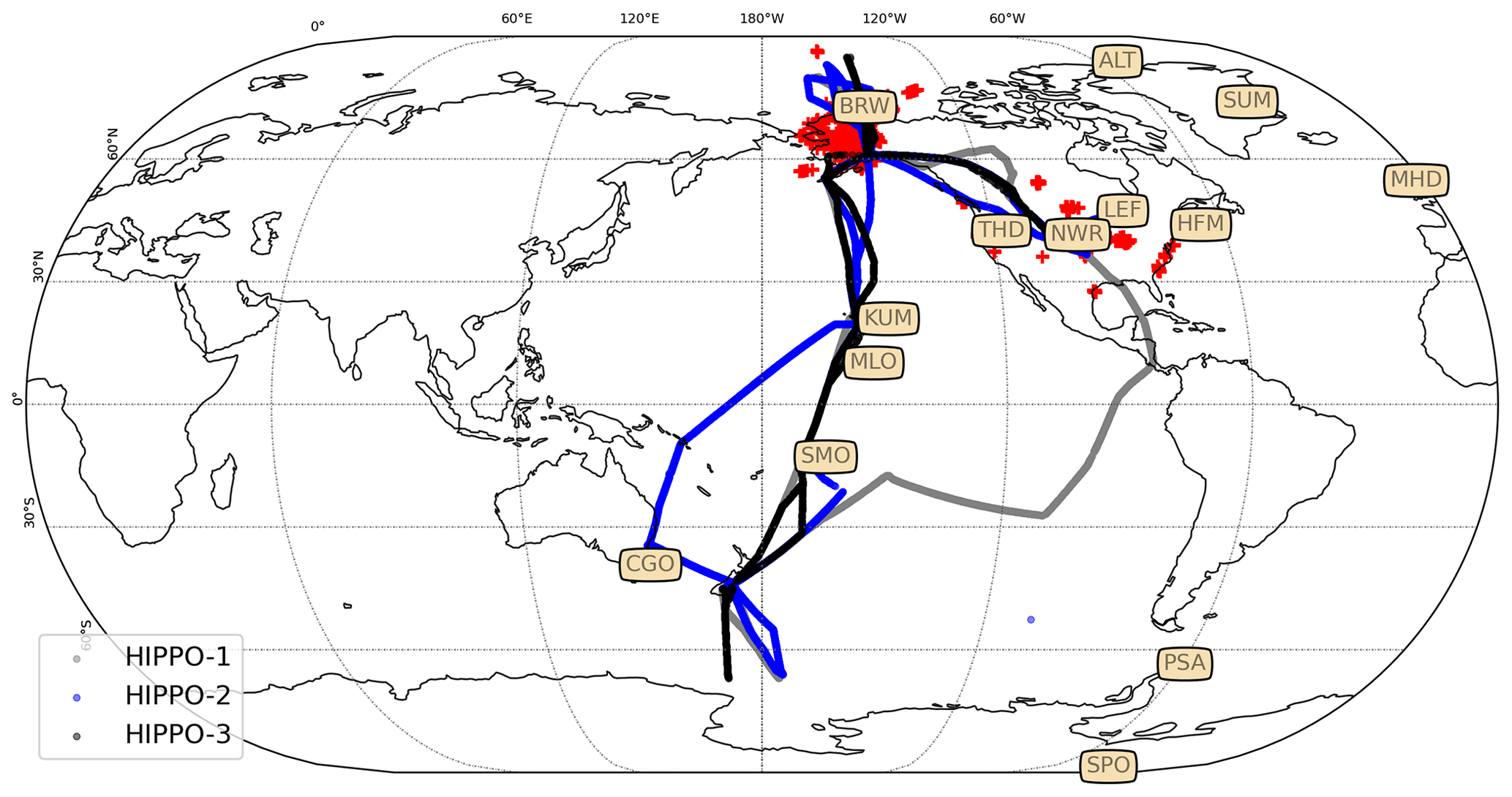
Figure 1Measurement data locations in this study. HIPPO campaigns 1–3 are shown as coloured flight tracks. NOAA airborne data are shown as red crosses. NOAA stations are marked on the map with station names.
2.1 NOAA surface network
The Global Monitoring Laboratory (GML) of the National Oceanic and Atmospheric Administration (NOAA) conducts continuous surface measurements at many sites globally and provides long-term ground-based measurement data that are suitable for inverse modelling studies. COS has been measured over 14 observational sites since 2000 to the present day (Montzka et al., 2007). The sites are depicted in Fig. 1.
Among the 14 measurement sites, 10 of them are located in the Northern Hemisphere (NH) and 4 in the Southern Hemisphere (SH). Of these sites, 3 are purely oceanic sites (MLO, KUM and SMO) suitable to sample oceanic emissions. SMO is located in the middle of the South Pacific between Hawaii and New Zealand. Another important station, MLO, is located on the north side of Mauna Loa volcano, Hawaii, at an elevation of 3397 m a.s.l. The KUM station also samples air from the ocean at Hawaii, but at sea level. From the perspective of inverse modelling, locations in the SH or over oceans are important because they measure COS mole fractions from pristine areas or from the marine atmosphere. In contrast, sites over land are useful to trace COS observations influenced by the biosphere or soil exchange and to trace sources from anthropogenic emissions and biomass burning. The COS measurements are taken on a weekly or bi-weekly timescale, with an average measurement error of less than 8 pmol mol−1 (Montzka et al., 2007). The measurements are calibrated to maintain data consistency amongst NOAA sites. It is worth noting that the coverage of the NOAA surface network for COS is sparse, which leads to challenges for inverse modelling. The total error used in inverse modelling includes the measurement error, the station-dependent representation error and the flux error (Ma et al., 2021).
2.2 MIPAS satellite
The Michelson Interferometer for Passive Atmospheric Sounding (MIPAS) was a Fourier-transform spectrometer that flew on the Environmental Satellite (Envisat) mission. MIPAS was a limb sounder, designed to detect a wide range of gases between the upper troposphere and lower thermosphere. The data sets retrieved by the European Space Agency from calibrated MIPAS spectra include profiles of temperature, H2O, O3, CH4, N2O, HNO3 and NO2 (Fischer et al., 2008). The MIPAS COS data set used here (V5R_OCS_221/222) was retrieved with the level-2 data processor developed and operated by the Institute for Meteorology and Climate Research (IMK) in cooperation with the Instituto de Astrofìsica de Andalucìa (IAA). COS retrievals from MIPAS data were characterised and compared with other data sets, showing that COS retrievals from MIPAS are good-quality measurements that reveal COS surface exchange processes (Glatthor et al., 2015, 2017). The data sets from MIPAS are available from 1 July 2002 to 8 April 2012.
The MIPAS COS data consist of volume mixing ratio profiles, averaging kernels and geophysical information (temperature, latitude, longitude, altitude, etc.). To compare modelled COS mixing ratios to MIPAS soundings the averaging kernel is applied as
where A is the MIPAS averaging kernel (AK, with dimension 60×60) matrix that contains information about the vertical sensitivity, xmodel is the profile sampled from a transport model, xprior is the prior profile and xconv is the model profile convolved with the AK. In practice, the prior for MIPAS COS retrieval is a zero profile, so Eq. (1) simplifies to
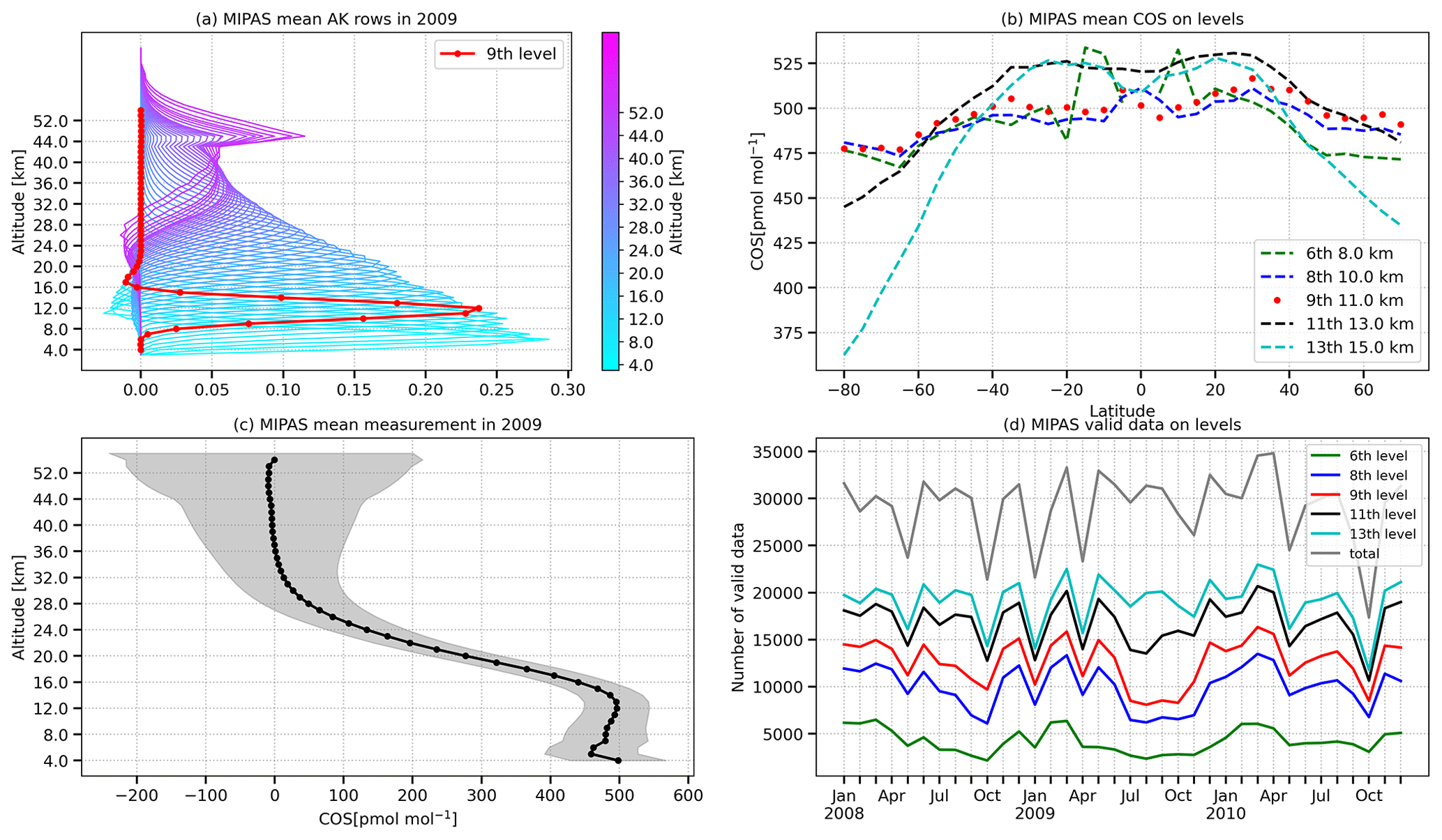
Figure 2Filtered MIPAS satellite data annual mean in 2009. (a) The selected MIPAS mean averaging kernel rows, coloured by their representative altitudes. (b) Selected MIPAS COS mean mole fractions on MIPAS levels (6, 8, 9, 11 and 13). (c) MIPAS mean COS vertical profile. (d) Number of valid measurements on selected MIPAS levels after data quality control.
The convolved COS mixing ratios are compared to MIPAS retrievals and then included in the cost function for inverse modelling. In this study with a focus on tropospheric COS, we only use the ninth level of the MIPAS COS retrievals. To make best use of the MIPAS data, we applied data quality control, and soundings that match one of the following criteria were removed. The purposes are indicated below.
-
To avoid cloud contamination, soundings with a MIPAS visibility flag of zero are discarded.
-
To avoid low sensitivity indicated by the AK, soundings with a diagonal element of the ninth AK row smaller than 0.03 are removed.
-
To avoid artefacts due to orography, soundings with a difference of more than 6000 Pa between the MIPAS reported surface pressure and the TM5 surface pressure are removed.
Figure 2 shows filtered MIPAS data analysis based on the annual mean of 2009. Panel (a) demonstrates that the ninth row of the AK roughly peaks at around 200 hPa, indicating a retrieval sensitivity to the troposphere, at least in the tropics. To motivate our selection for the ninth MIPAS level, panel (b) shows the latitudinal distribution of the MIPAS COS mole fraction at levels 6, 8, 9, 11 and 13. The MIPAS measurements for levels 6, 8 and 9 are relatively similar, but COS mole fractions drop quickly for level 11 and above, due to enhanced sensitivity to stratospheric COS, as shown in the mean COS profile in panel (c). Panel (d) shows the total number of valid MIPAS data after applying the data quality control. It is evident that the number of valid MIPAS soundings drops when the level is closer to Earth's surface, due to the influence of clouds. In summary, the ninth MIPAS level is chosen to best represent tropospheric COS while still retaining a substantial number of valid measurements.
2.3 Validation observations
Since the COS inverse problem is data-constrained, independent data are crucial to further validate the inversion results, particularly with respect to the modelled vertical distribution. This is particularly true when assimilating surface observations combined with MIPAS data, which have the highest sensitivity in the upper troposphere. For clarification, independent or validation data refers to observations that are not assimilated in the inverse model. In principle, evaluation with independent observations can help in pinpointing potential model errors or poorly estimated flux adjustments.
HIAPER Pole-to-Pole Observations (HIPPO) data provide valuable and well-calibrated COS concentrations between January 2009 and September 2011, a period with valid MIPAS data. HIPPO data were collected during several campaigns (see Fig. 1) between the surface and the tropopause and from the NH to the SH (Wofsy, 2011; Wofsy et al., 2017). HIPPO COS measurements were evaluated to be consistent with the NOAA surface network. We use data from HIPPO campaigns 1–3 to validate the inversion results. Next to HIPPO data, we use NOAA airborne profile data that are routinely collected. Most profile measurements are taken in North America, shown in Fig. 1 as red crosses.
Inverse modelling is a widely used mathematical technique to estimate surface fluxes of trace gases, constrained by concentration observations at ground level or from space. The inverse model usually consists of a transport model and an observational system, coupled to an optimiser that minimises the difference between observations and model results by changing the emissions. The transport model describes physical and chemical processes: advection in three dimensions, parameterisation of deep convection and other sub-grid-scale mixing processes, and chemistry (Krol et al., 2005). The observational system in this study includes the NOAA surface network and MIPAS data, and these data provide constraints to estimate surface fluxes of COS and CS2. Note that we do not optimise DMS surface fluxes in this study.
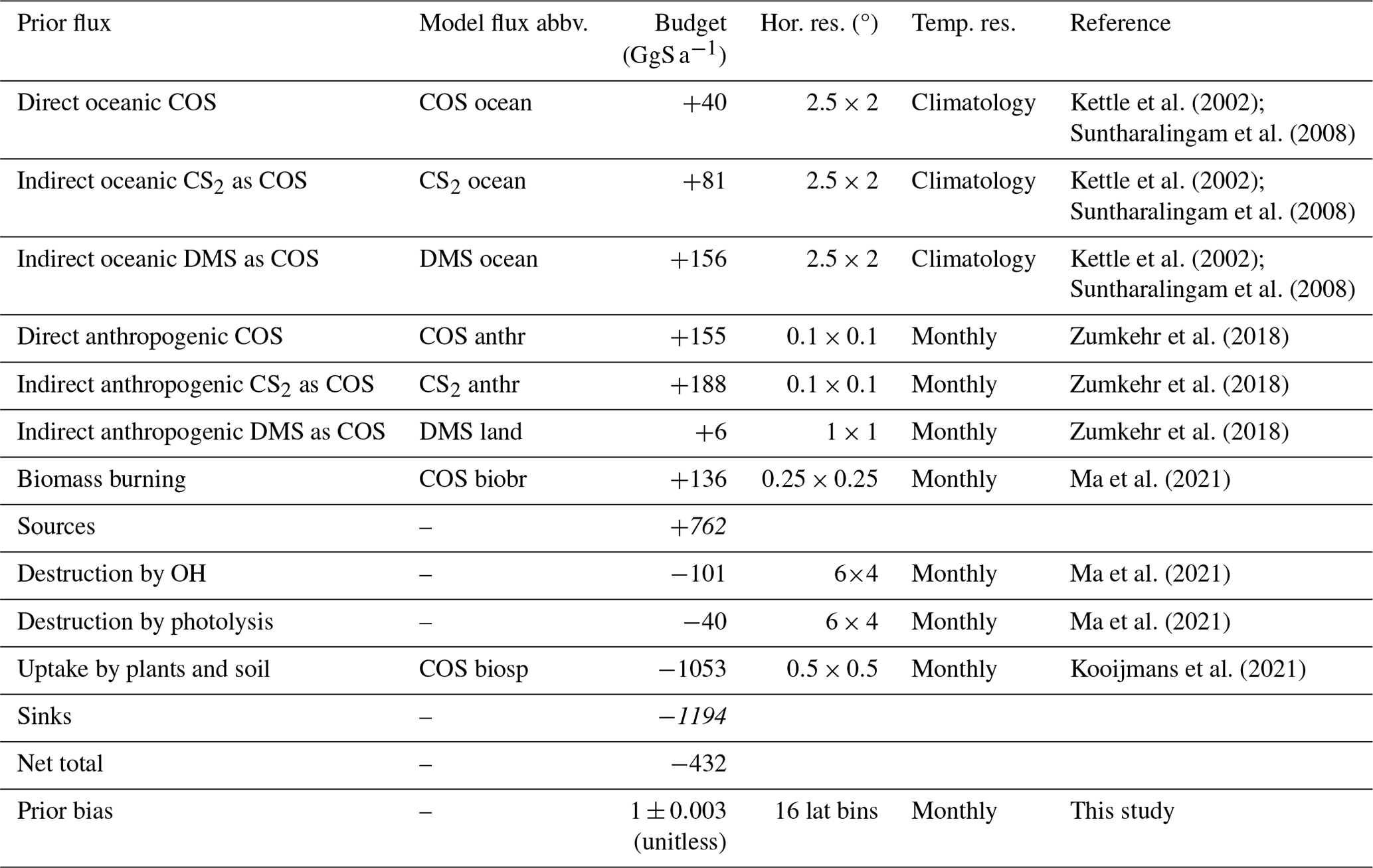
Kettle et al. (2002)Suntharalingam et al. (2008)Kettle et al. (2002)Suntharalingam et al. (2008)Kettle et al. (2002)Suntharalingam et al. (2008)Zumkehr et al. (2018)Zumkehr et al. (2018)Zumkehr et al. (2018)Ma et al. (2021)Ma et al. (2021)Ma et al. (2021)Kooijmans et al. (2021)Table 1Description of inversion settings, prior fluxes and prior bias correction. Italics are used to show the sources and sinks of COS. These are the sum of all sources or sinks.
3.1 Prescribed surface fluxes of COS, CS2 and DMS
In the model implementation, we used the prior surface fluxes of the three tracers from Ma et al. (2021). Here, four categories are predefined for COS surface fluxes: anthropogenic, biosphere, ocean and biomass burning. We briefly describe these fluxes below, and prior flux information is listed in Table 1.
The reported anthropogenic COS emissions range between 223–586 GgS a−1 (Zumkehr et al., 2018) in the period 2000–2012. Specifically for 2009, the focus year of this study, the emissions amount to 354.2 GgS a−1. The anthropogenic sources are available as monthly estimates on a high spatial resolution of 0.1°×0.1°. Furthermore, the Zumkehr et al. (2018) inventory reports direct COS and CS2 emissions, and we used the CS2-to-COS ratios of the various emission types to split emissions into direct COS emissions and indirect CS2 emissions following Table 1 of Lee and Brimblecombe (2016). In addition, a small amount of DMS emissions over land (6 GgS a−1) is also regarded as an indirect COS source. DMS and CS2 are treated as separate tracers that are quickly oxidised to COS (see below). The biosphere flux is the largest sink for COS and includes uptake by plants and soil at the surface. Here, we use the output generated by the SiB4 model (Kooijmans et al., 2021) from 2000 to 2020 to drive the TM5 model, in order to account for the inter-annual variability in biosphere uptake. These fluxes are still evaluated assuming a constant atmospheric COS mole fraction of 500 pmol mol−1. This leads to a prior flux estimate of −1053 GgS a−1. Fluxes are provided as monthly fields on a 1°×1° resolution. Ocean fluxes of COS, CS2 and DMS are based on climatological fields (Kettle et al., 2002; Suntharalingam et al., 2008; Lana et al., 2011). The COS oceanic flux depends on sea surface temperature and can thus be either a source or a sink, depending on the season. COS biomass burning emissions considered biomass burning and biofuel use, with an amount of 136 GgS a−1 (Ma et al., 2021).
3.2 Chemistry
The chemical conversion of CS2 and DMS is handled as described in Ma et al. (2021). Briefly, CS2 is converted to COS through a reaction with OH assuming a yield of 0.83 (Stickel et al., 1993). DMS is converted to COS using a yield of 0.007 (Barnes et al., 1994) assuming an exponential decay to COS with a timescale of 1.2 d (Khan et al., 2016). Recent studies found a new DMS oxidation product, HPMTF, which potentially plays a role in COS production (Wu et al., 2015; Veres et al., 2020; Fung et al., 2022; Jernigan et al., 2022). Here, we still use the assumption of a 0.7 % yield from DMS oxidation (Barnes et al., 1994). Note that the reaction rate of COS and OH quoted in Ma et al. (2021) contained a typo. Here we give the correct equation:
where T is temperature in K and A is pre-exponential factor of the Arrhenius equation ( cm3 s−1 molecule−1) for the reaction of COS with OH (Cheng and Lee, 1986). As in Ma et al. (2021) we used the OH climatology by Spivakovsky et al. (2000) multiplied by 0.92 in the troposphere.
3.3 TM5-4DVAR system
TM5-4DVAR is an offline global inverse model using 4DVAR data assimilation techniques (Krol et al., 2005, 2008; Meirink et al., 2008; Bergamaschi et al., 2010). The 3 h meteorological fields from the European Centre for Medium-Range Weather Forecasts (ECMWF) ERA-Interim reanalysis is employed to drive the offline TM5 model (Dee et al., 2011). The TM5 transport model describes the physical transport of tracers by atmospheric winds and their chemical loss and production. The model settings are identical to Ma et al. (2021). The difference is that the MIPAS observations are assimilated into the inverse system and that a bias correction scheme is implemented.
The forward model consists of a transport operator and an observation operator that acts on a state vector x:
The TM5 model (H) simulates the mole fraction of COS, after which the misfit between model and measurement (surface and/or satellite) is calculated, co-sampled in space and time. In this study the operator is linear, and Eq. (3) can be written as Hx. The value of the cost function J (Eq. 4) is calculated with the forward model, and the derivative of the cost function with respect to the state vector elements is calculated with the adjoint model HT. An optimisation algorithm is used to minimise the cost function up to a predefined gradient reduction. Equation (4) is a classic form of a cost function in an inverse system (Tarantola, 2005; Brasseur and Jacob, 2017):
and the derivative of the cost function with regard to the state vector x reads
where x is the state vector to be optimised and xb is the prior state vector. The covariance matrix B describes the uncertainty statistics associated with the state vector. The covariance matrix R describes errors related to the misfit between observations and the model (Hx−y). While R is (often) assumed to be diagonal, off-diagonal elements of B are determined by user-prescribed spatial and temporal correlations of the fluxes (details of the correlation lengths used can be found in Ma et al., 2021). The inverse of B is not explicitly calculated owing to its huge size, but it is dealt with during pre-conditioning and eigenvalue decomposition (Meirink et al., 2008).
Our implementation of TM5-4DVAR runs on a spatial resolution of 6×4° horizontally and on 25 pressure levels vertically. Fluxes are optimised on a monthly timescale. In this study, we focus on a 3-year inversion from 1 January 2008 to 1 January 2011. The initial condition is based on a previous 3-year inversion in which atmospheric COS was spun up using atmospheric surface observations. The inversion model optimises all COS and CS2 fluxes but keeps the DMS fluxes constant, as per scenario S1 described in Ma et al. (2021). Since the inverse system remains linear, including the comparison to MIPAS satellite data, we use the CONGRAD algorithm (Lanczos, 1950) to optimise the fluxes until the gradient norm is reduced by a factor of 10−7. We found that, with this convergence criterion, the leading eigenvalue of the Hessian of the cost function is close to 1.0, which implies that both the fluxes and the posterior errors can be reliably interpreted (Meirink et al., 2008). Using the posterior covariance matrix, the error reduction (ER, defined in Eq. 6) and correlations of the optimised fluxes can be evaluated.
where errorprior and errorposterior are the errors of posterior and prior fluxes and are also the diagonal elements in the B matrix defined in Eq. (4). According to Meirink et al. (2008), the posterior error must be smaller than the prior error, leading to an error reduction for an inverse system. We report correlations and error reductions of COS and CS2 fluxes based on error aggregation over NH lands, NH oceans, SH lands and SH oceans during the period of 2009 in Sect. 4.5. The first six months in 2008 and the last six months in 2010 are considered as spin-up and spin-down periods respectively. At the beginning of the inversion, the optimised fluxes may be affected by the uncertain initial condition. At the end of the inversion, there are fewer observational data to constrain fluxes. We believe that the spin-up and spin-down approach improves the statistics of the inversion.
3.4 Bias correction
A bias may exist amongst different measurement streams, e.g. between the NOAA surface network and the MIPAS satellite data. This bias may be due to different instruments or calibration methods. In addition, since some of the sensitivity of the MIPAS data extents to the stratosphere (see Fig. 2a), some bias may be introduced by incorrect transport to, and chemistry in, the stratosphere. A bias correction scheme may successfully correct for systematic satellite measurement biases (Monteil et al., 2013; Houweling et al., 2014). To correct for potential biases, we implemented a bias correction to MIPAS data with monthly and latitudinal variations. The prior values of the bias correction are assumed to be 1.0, i.e. no bias existing between different measurement systems. The cost function of the state vector of surface fluxes can be extended with a bias correction as
The derivative of the cost function with respect to the bias terms, β, then becomes
In these equations, RMIPAS and RNOAA are the error covariance matrices associated with NOAA surface observations and MIPAS data respectively. β is the bias correction parameter assigned to MIPAS measurements, and γ is a regularisation factor, which scales the MIPAS data part of the cost function. Equation (8) relates the MIPAS error inflation to γ. The assumption here is that NOAA surface observations and MIPAS profiles are all independent so that the error covariance matrix for all data in Eq. (4) is diagonal and can be separated into two matrices. The regularisation factor is similar to the terminology defined in Brasseur and Jacob (2017). In our case, the number of MIPAS measurements (127 243 in 2009 after data quality control) overwhelms the number of NOAA surface observations (490 in 2009), and the error inflation is a factor that limits the weight of MIPAS data in the cost function. Note that the error inflation can also account for potential correlations between the various MIPAS soundings. We determined that an error inflation of leads to a reasonable balance between MIPAS and NOAA terms in the cost function.
The derivative with regard to β (Eq. 9) is implemented in the data assimilation system, such that β is simultaneously optimised along with the fluxes. As discussed in Sect. 2, we selected the ninth level of MIPAS data near 200 hPa to be assimilated in the system. In the assimilation, a mass conservation mapping algorithm is used to map the 25 TM5 pressure levels to the 60 MIPAS levels.
The bias parameters β are multiplied with the MIPAS observations (Eq. 7). The prior values of bias parameters are set to 1.0±0.003 as shown in Table 1. The small error assigned to bias parameters is to prevent the MIPAS data from being adjusted too strongly. We furthermore assume that the MIPAS bias depends on month and latitude, not on longitude. The monthly and latitudinal bias corrections are assumed to be correlated by decay functions that fall off in space and time. For the latitudinal variations, a Gaussian decay function is selected:
where ilat and jlat are the two correlated latitude indices and bin is the bin size that determines how many bins are taken into account. For MIPAS we take into account the latitude range from 80° S to 80° N, and 16 latitude bins are applied, so bin is equal to 10°. L is the spatial correlation length, which is set to 5°. For the temporal correlation, an exponential decay is assumed:
where imonth and jmonth are the two correlated month indices and τ is the temporal correlation length, taken as 9.5 months. Finally, the covariance matrix Bβ is written as a Kronecker product of Eqs. (10) and (11).
3.5 Evaluation metrics
To evaluate the performance of the inverse system, it is important to compare the model with assimilated and unassimilated data, e.g. either ground-based observations or satellite observations. We use the statistical metrics χ2 to characterise the performance of the inversions by comparing the surface network observations and inversion results.
When the observations are assumed independent, χ2 is twice of the cost function (Tarantola, 2005):
In a well-balanced inverse problem, is equal to the number of observations N. Since the background part of the cost function is usually small, and we are interested in the performance of the inversion at different stations, we prefer to use the station-based χ2 to characterise the performance of inversions. For comparison between model results and NOAA stations, the station-based χ2 is defined as
where i denotes the ith station and N is the number of observations at that station. Note that a χ2 of 1 denotes a statistically good fit to the available observations; i.e. the difference between the model result and measurements is the same size as the spread of the observations. For comparison between model and satellite data, χ2 is also used to compare the modelled and MIPAS-measured COS without taking the error inflation in order to avoid small values of the satellite χ2.
In this study we also analyse regional correlation and error reduction on various spatial and temporal scales, as outlined in Sect. 3.3. Aggregation to different scales is performed by accounting for the covariance from the full prior and posterior covariance matrices. Results will be presented in Sect. 4.4 and 4.5.
Table 2Prior errors applied in the inversion scenarios in this study. The percentage is the prior error assigned to the prior fluxes. DMS remains the prior value and is not adjusted during optimisations. Note that the absolute grid-scale flux error also depends on the flux quantity, which means that 10 % error to the biosphere is larger than the same error to anthropogenic COS.
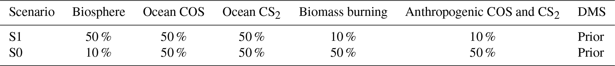
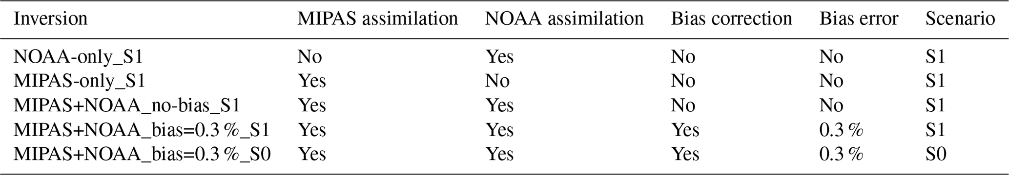
Table 3Inversions carried out in this study. The parameters are presented as MIPAS or NOAA assimilation, bias correction and bias error. The inversion names are used to denote the experiment throughout the paper.
3.6 Overview of inversions
To explore various model settings and simulation scenarios, we have designed a set of inversions, shown in Tables 2 and 3. The inversion scenario labelled S1 represents a similar setting to that used in Ma et al. (2021), with 50 % prior errors for the COS biosphere fluxes and for the COS and CS2 ocean fluxes. To investigate the impact of the prior error settings on the posterior biosphere fluxes, in scenario S0 the biosphere error was reduced to 10 %, while the COS anthropogenic and biomass burning emission errors were increased from 10 % to 50 %. For scenario S1, we assimilate only NOAA surface observations (NOAA-only_S1), only MIPAS data (MIPAS-only_S1), and both observational data sets with (MIPAS+NOAA_bias=0.3 %_S1) and without bias correction (MIPAS+NOAA_no-bias_S1). For scenario S0, we only consider assimilation of NOAA and MIPAS data with bias correction (MIPAS+NOAA_bias=0.3 %_S0). Since we do not know the “true” MIPAS bias, a bias-corrected MIPAS-only inversion is difficult to perform and is not presented.
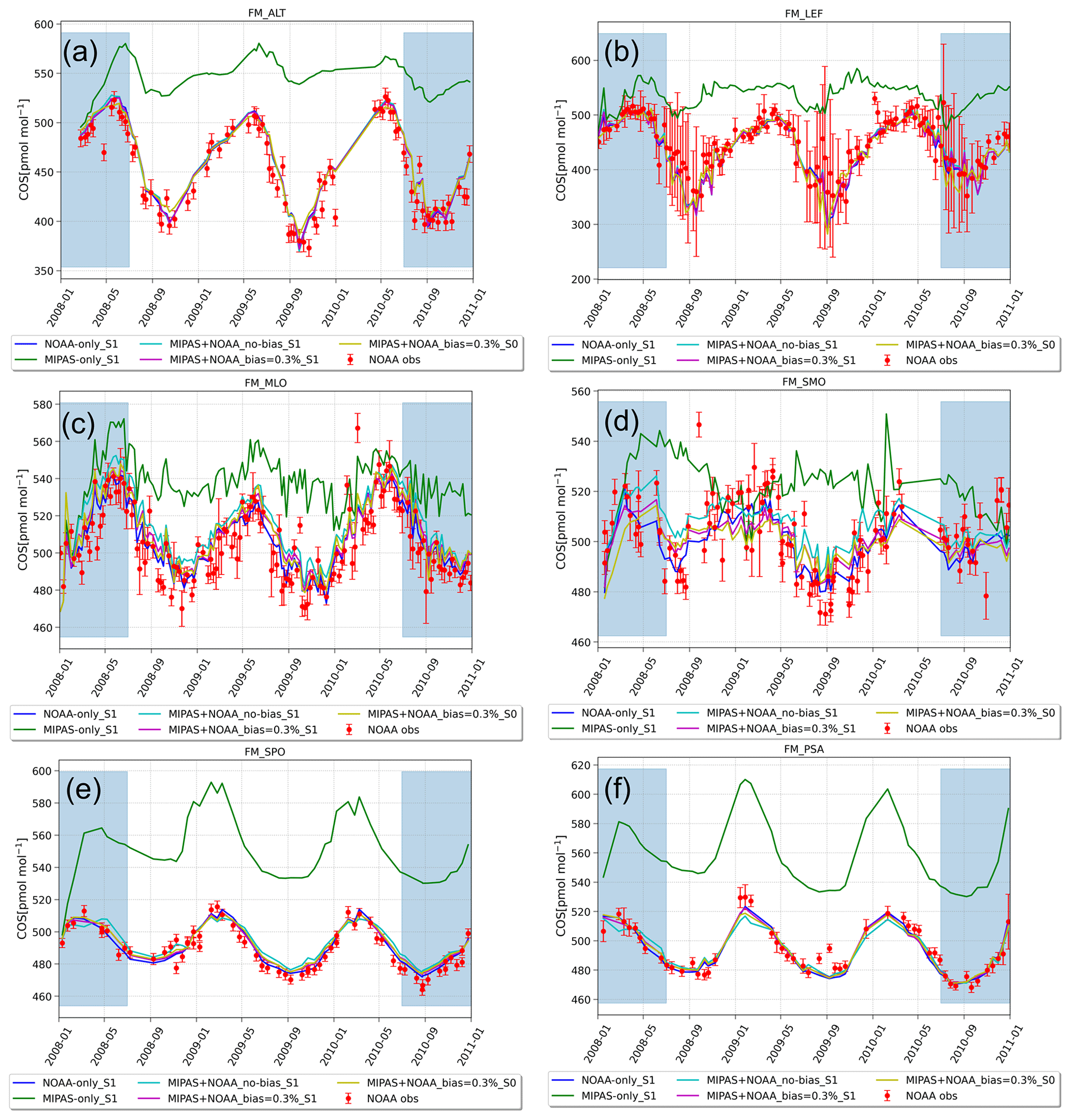
Figure 3NOAA surface measurements at selected stations and modelled COS mole fractions of inversions. The NOAA surface observations are plotted as red dots with their total error, and modelled COS mole fractions are plotted as solid lines. The first and last 6 months are shaded in blue as spin-up and spin-down periods respectively.
4.1 Posterior fit to observations
To demonstrate the performance of each inversion, we first evaluate the posterior fit at the 14 NOAA surface stations. Figure 3 compares the various inversions at 6 selected stations. At Alert (ALT; Fig. 3a), MIPAS-only_S1 severely overestimates COS observations, while the other inversions that assimilate NOAA data match the observations well. The same pattern is found at station LEF (Fig. 3b). However, the posterior fit is not as good at oceanic stations MLO and SMO (Fig. 3c and d). Here, the best results are obtained for the NOAA-only_S1 inversion, which is logical because only NOAA surface data are assimilated. When MIPAS data are also assimilated, the model fit at MLO and SMO deteriorates, which implies trade-offs between assimilation of surface and MIPAS data. At the Antarctica stations SPO and PSA (Fig. 3e and f) the model fit improves again. Overall, the MIPAS-only_S1 inversion overestimates COS mixing ratios at all surface stations. This is the result of the low sensitivity of MIPAS to COS that resides close to the surface. It also indicates that MIPAS information is highly biased within the TM5-4DVAR system. As outlined above, this might imply a lack of observations to constrain the model or a bias in the model transport and chemistry. However, a true bias of MIPAS compared to NOAA observations cannot be excluded. Glatthor et al. (2017) also found positive differences of MIPAS retrievals compared to ACE-FTS profiles in the upper troposphere and lower stratosphere.
To evaluate the performance of the various inversions (except for MIPAS-only_S1) at each NOAA station, Fig. 4 shows χ2 per station (Eq. 13). The stations are sorted from south to north. As expected, the best performance is found for NOAA-only_S1 (in blue). Values of χ2 close to 1 are found for CGO, LEF and MHD. Reasonable results are obtained at the other stations, with χ2 values less than 5. Although the agreement with observations improves considerably with regard to the prior (not shown), this could indicate that error settings for these stations were too conservative, possibly related to unaccounted processes that influence the COS budget. Indeed, we note considerable variability at remote ocean stations, such as MLO and SMO (see Fig. 3), that is not reproduced well by the model.
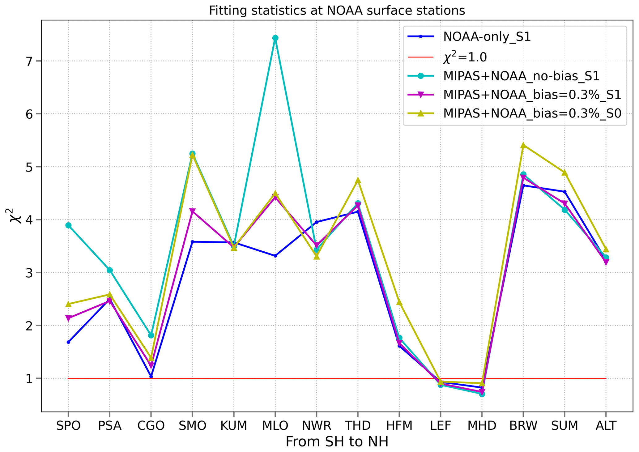
Figure 4Inversion metric χ2 (Eq. 13) at each NOAA surface station for all inversions except MIPAS-only_S1. The red line denotes χ2=1.
In Fig. 4, the worst performance is found for inversion MIPAS+NOAA_no-bias_S1 (excluding the MIPAS-only inversion), with a deteriorated model fit especially at SMO and MLO. When bias correction is applied in inversion MIPAS+NOAA_bias=0.3 %_S1, the model fit improves at all NOAA stations. When the prior errors are reduced for the biosphere flux (and increased for the anthropogenic and biomass burning fluxes in inversion MIPAS+NOAA_bias=0.3 %_S0), the posterior fit degrades at most stations, except for MLO. This indicates that adjustments of the biosphere fluxes play an important role in the goodness of the posterior fit. However, alternative choices of the prior error setting (e.g. scenario S0) still lead to satisfactory results.
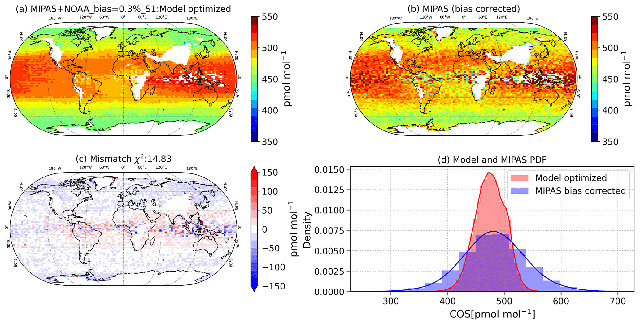
Figure 5Comparison of the MIPAS observations with the results of inversion MIPAS+NOAA_bias=0.3 %_S1. (a) Modelled COS at MIPAS level 9. (b) Bias-corrected MIPAS observations in the upper troposphere (MIPAS level 9). (c) Mismatch derived from panel (a) minus panel (b). (d) Probability density function of the modelled and MIPAS COS mole fractions.
Next we evaluate the posterior fit to MIPAS data. The posterior model fit with MIPAS data for inversion MIPAS+NOAA_bias=0.3 %_S1 is shown in Fig. 5. The mismatch (panel c) shows that the model, after bias correction, still slightly underestimates MIPAS COS mixing ratios at high latitudes and overestimates values over tropical regions. As expected from assimilated observations, the probability density function (panel d) indicates that the average modelled COS mixing ratio is relatively close to the MIPAS average. However, due to the large error on individual MIPAS soundings, the distribution of MIPAS is much wider. Supplement Figs. S1 and S2 show the posterior model fit with MIPAS data for inversion MIPAS-only_S1 and MIPAS+NOAA_no-bias_S1, respectively, where the bias correction scheme is not applied. In the case of MIPAS-only_S1, the MIPAS-based χ2 amounts to 16.4, and, in the case of MIPAS+NOAA_no-bias_S1, the χ2 increased to 17.33. This implies that when both NOAA and MIPAS are assimilated, the fit is deteriorated to some extent. Interestingly, in the case of MIPAS+NOAA_bias=0.3 %_S1, the fit to MIPAS improved (χ2=14.8). In general, inversion MIPAS+NOAA_bias=0.3 %_S1 reached an acceptable posterior model fit both at NOAA surface stations and to MIPAS data that are sensitive to the upper troposphere.
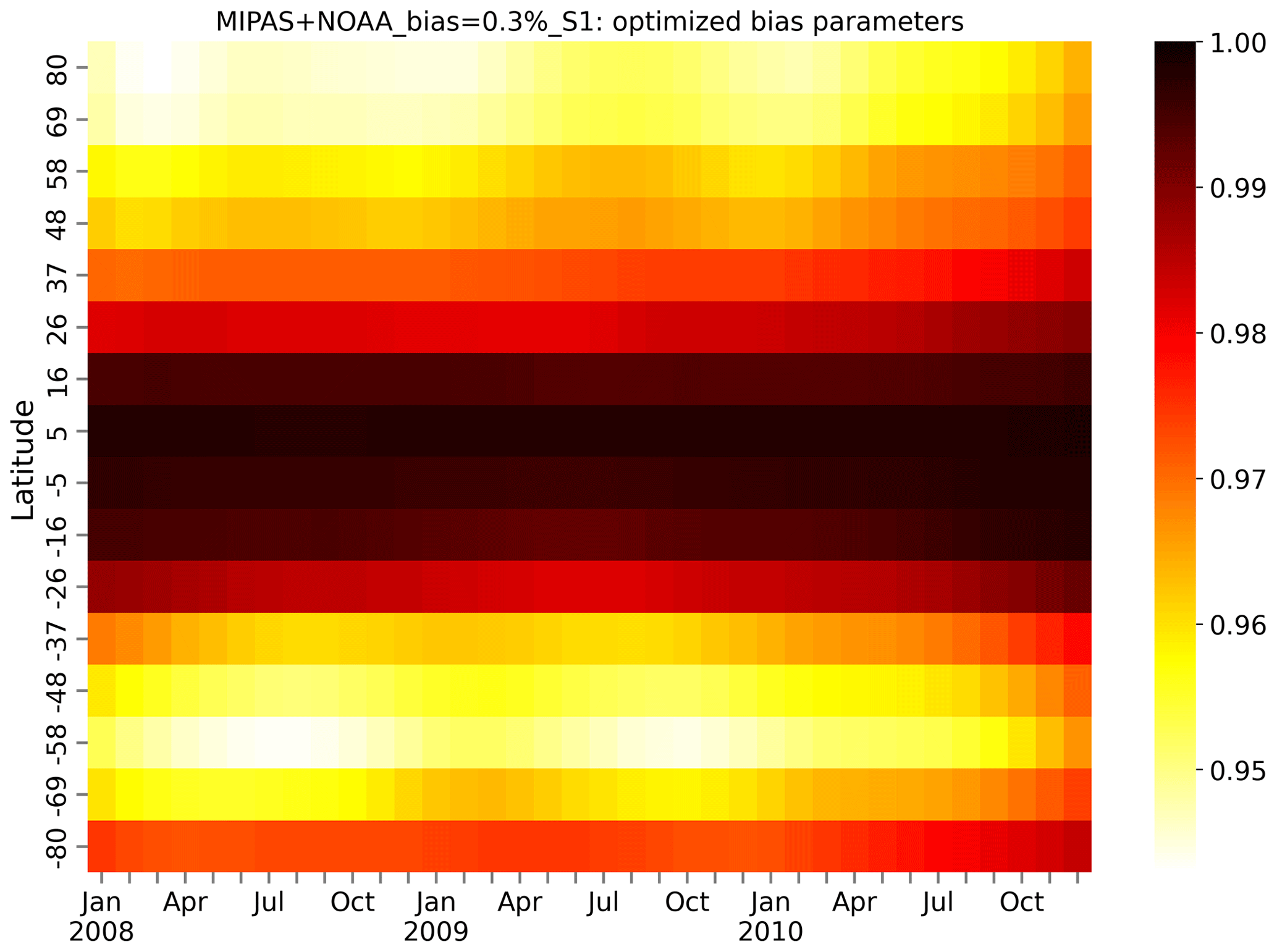
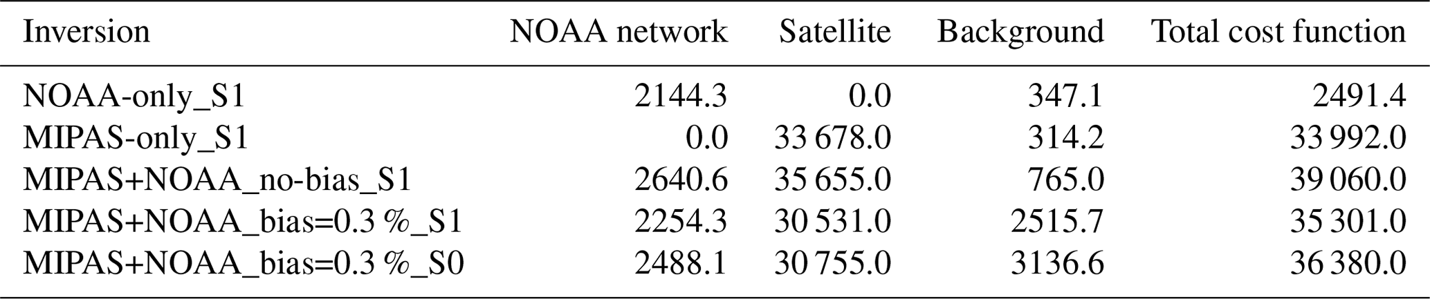
Table 4Breakdown of the cost functions of the five inversions. The costs are given for the NOAA network, MIPAS satellite data and the background term respectively.
4.2 Optimised bias correction parameters
Figure 6 shows the posterior bias parameters as a function of month and latitude for inversion MIPAS+NOAA_bias=0.3 %_S1. The posterior bias parameters are in the range 0.94–1.00, indicating that bias correction slightly reduces MIPAS observations in order to reconcile the fit to surface observation. In the tropics, only a small bias correction is found, while higher latitudes show larger corrections. At these latitudes there is also a slight seasonal cycle in the bias parameters, with larger corrections in local winter. Since in local winter high-latitude MIPAS observations are mostly sensitive to the stratosphere, this could indicate potential model errors in transporting COS to the stratosphere. The other inversion scenario (S0, not shown) shows similar posterior bias parameters within the range of 0.94–1.0 with similar seasonal and latitudinal variations. The bias correction parameters are not adjusted to reduce biases in tropical regions, and the reasons could be as follows: (1) mixing is fast in the tropics, and transport and chemistry errors are much smaller. (2) At higher latitudes, MIPAS samples pressure levels in the stratosphere, where the air is older. Thus, transport errors and errors in modelled COS breakdown become more important. (3) The MIPAS data quality is better over the tropics.
To show the overall performance of all inversions, Table 4 breaks down the cost function in terms of background costs, NOAA costs, and MIPAS costs. The background part contains both the flux part and the costs associated with bias correction (see Eq. 7). Inversion NOAA-only_S1 has the smallest posterior cost, since only deviations with surface observations are taken into account. For this inversion, the background costs are 15 % of the model–data mismatch. Whenever MIPAS data are assimilated, the satellite cost function becomes the dominant part, even though an error inflation of is considered. It is instructive to look at the increase in the background term when bias correction is considered (MIPAS+NOAA_bias=0.3 %_S1 and MIPAS+NOAA_bias=0.3 %_S0). As expected within an inverse modelling framework, this increase in background costs is more than compensated by reductions in both the MIPAS costs and surface costs. It also shows that additional adjustments to the fluxes are made to comply with both the surface and satellite data.
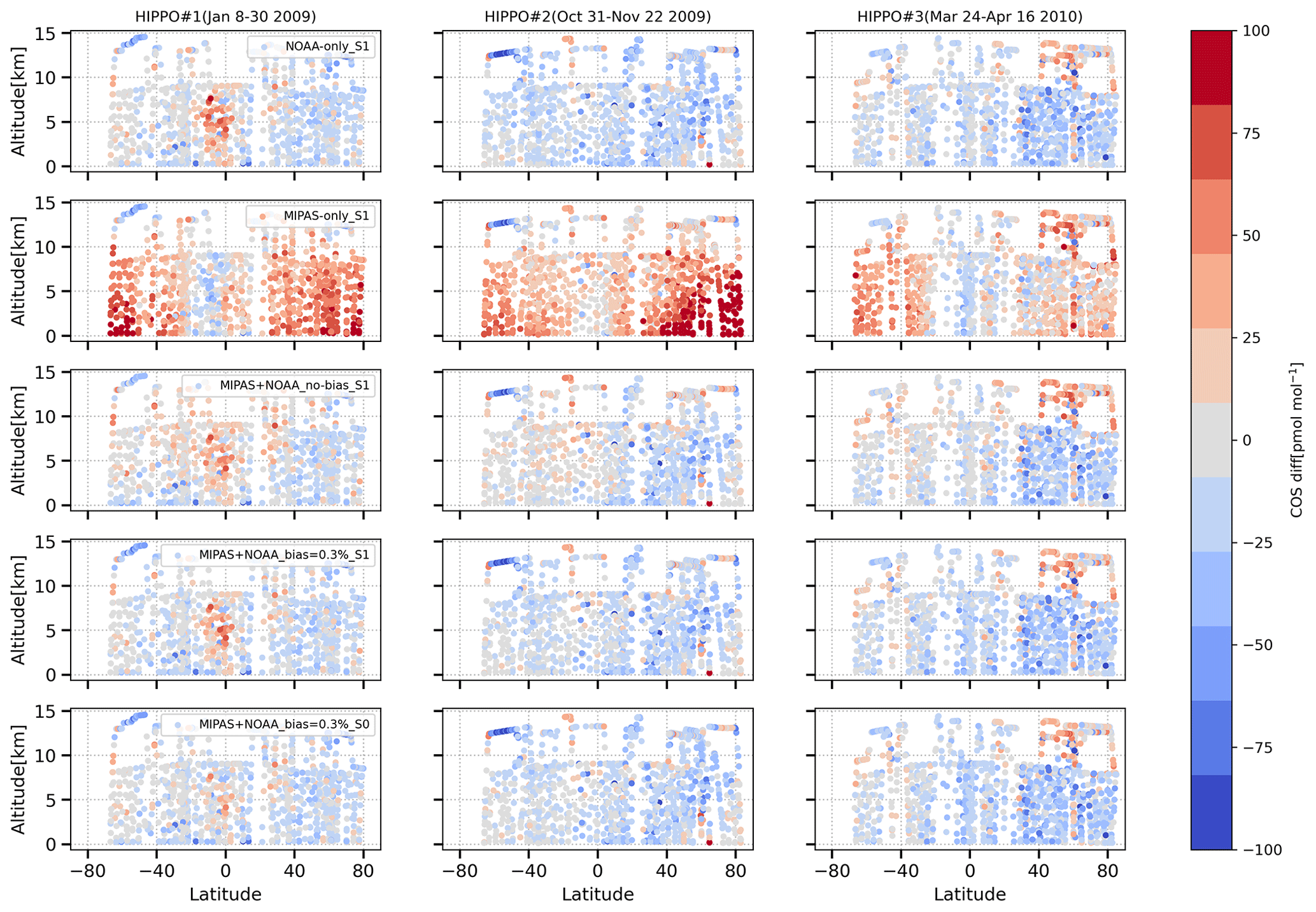
Figure 7Comparison of inversions with HIPPO observations as a function of latitude and altitude. The plotted results are modelled COS minus HIPPO observations. The rows denote the five inversions labelled in the left-hand column.
4.3 Validation with HIPPO and NOAA airborne profiles
In this section, independent HIPPO and NOAA airborne profile observations are used to evaluate the inversions. The evaluation of HIPPO campaigns 1–3 is shown in Fig. 7. Notably, as can be seen in the first two rows of Fig. 7, the NOAA-only_S1 inversion underestimates COS in the troposphere, while inversion MIPAS-only_S1 generally overestimates COS in the lower troposphere. The other inversions that assimilate MIPAS data decrease the bias against HIPPO observations. One remarkable feature in the comparison with HIPPO campaign 1 in January 2009 is the model overestimation around the Equator that gets reduced in inversion MIPAS+NOAA_bias=0.3 %_S0. This is caused by smaller biosphere flux adjustments that are the result of the tighter error settings (prior error reduced from 50 % to 10 %; see Table 2). The HIPPO 1 air samples were taken close to Amazonia (Fig. 1). This indicates that the adjustments to the biosphere over Amazonia in scenario S1 are likely too large. This will be addressed further in Sect. 4.4.
The vertical distributions of inversions and HIPPO observations are shown in Figs. S3 and S4. In HIPPO campaign 1, the vertical profiles of the inversions are in good agreement with HIPPO vertical distribution, with differences less than 20 pmol mol−1 below 10 km. For HIPPO campaigns 2 and 3, there is a negative bias between the inversions and the HIPPO observations. This points to underestimated oceanic contributions, as HIPPO campaigns 2 and 3 mainly covered the Pacific Ocean.
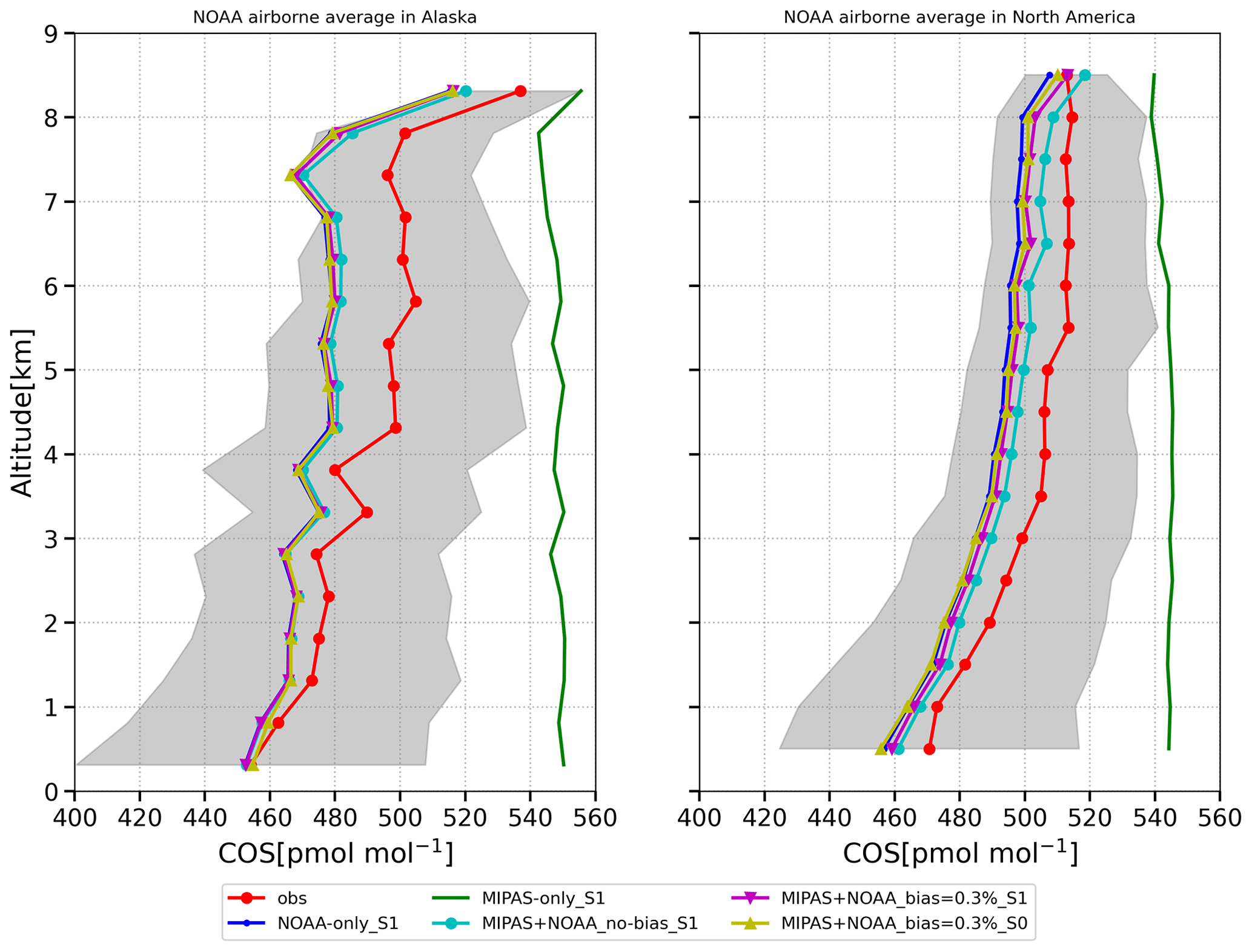
Figure 8Comparison of inversions with NOAA airborne profiles. The NOAA airborne data were separated into two regions: Alaska and North America. The airborne profiles are averaged vertically in 500 m intervals. The grey shading is the standard deviation of the NOAA airborne measurements within each vertical interval.
The evaluation against NOAA airborne profiles is presented in Fig. 8. Note that the data were grouped into two regions, Alaska and the rest of North America, as shown in Fig. 1. All inversions (except for MIPAS-only_S1) fit the profiles relatively well. Again, inversion MIPAS-only_S1 (in green) overestimates NOAA airborne observations significantly. Other inversions are generally slightly lower than the NOAA airborne observations, with slightly larger deviations when MIPAS bias correction is applied. The NOAA airborne profiles were mainly acquired over continents, where the inversions seem generally well-constrained by the NOAA surface network. Assimilation of MIPAS data does not strongly influence the agreement with the observed profiles. As shown in Fig. S5, we still find a low bias in our inversions, which, however, remains well below 20 pmol mol−1 over North America.
Table 5Prior and posterior fluxes and their error reductions for all inversions. Fluxes are given as flux ± error GgS a−1 (error reduction in %). The flux errors are aggregated for each region and flux category using the posterior covariance matrix. Note that DMS fluxes are not listed, since they are not optimised. The land and ocean fluxes are not strictly separated because the 6°×4° grid cells in coastal regions cover both land and ocean.
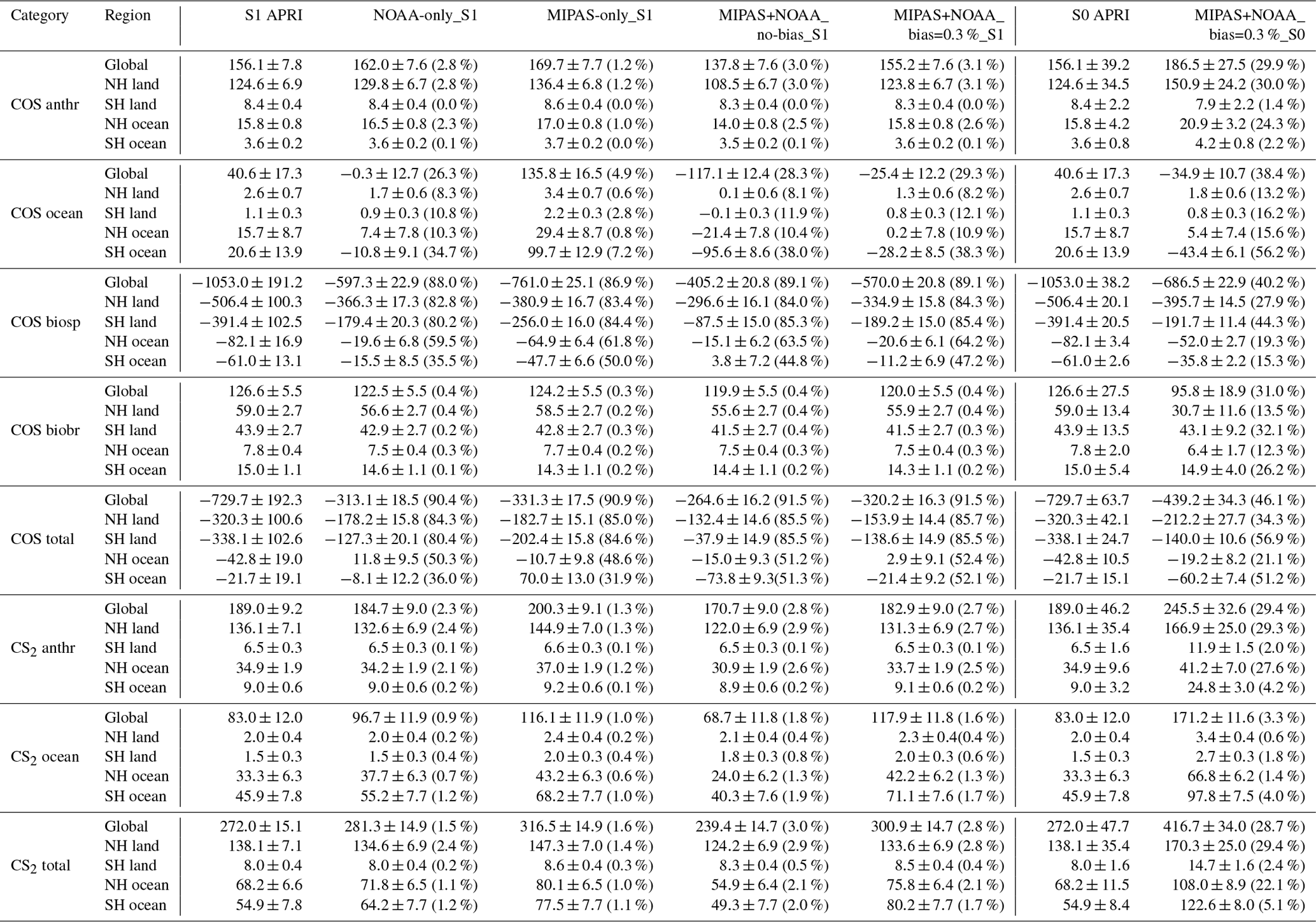
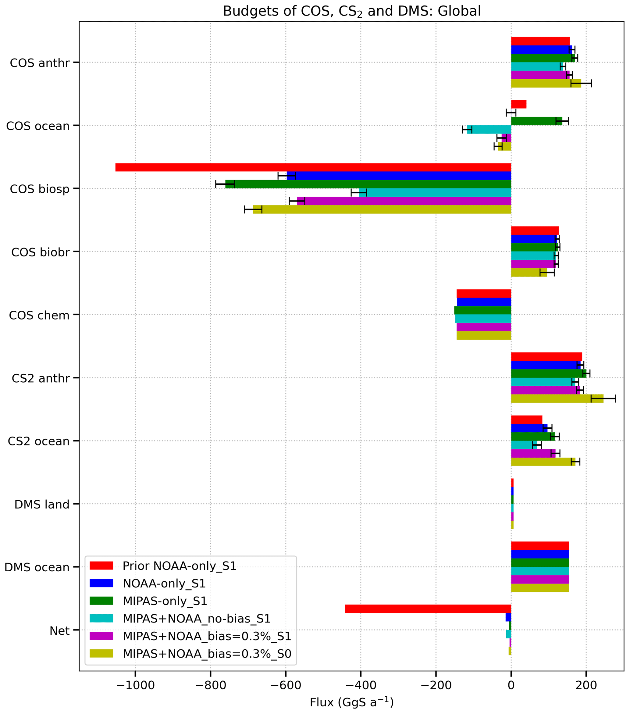
Figure 9Global COS budgets for the different inversions. The error bars represent the prior or posterior errors which are aggregated to the global scale. Note that the prior errors on the fluxes are not plotted because scenarios S1 and S0 have different prior errors. Note further that the CS2 and DMS budget terms are counted as indirect COS fluxes.
4.4 The global and Amazonia COS budget
The global COS budgets of all inversions are graphically summarised in Fig. 9. Furthermore, the regional prior and posterior COS and CS2 fluxes, errors, and error reductions are listed in Table 5.
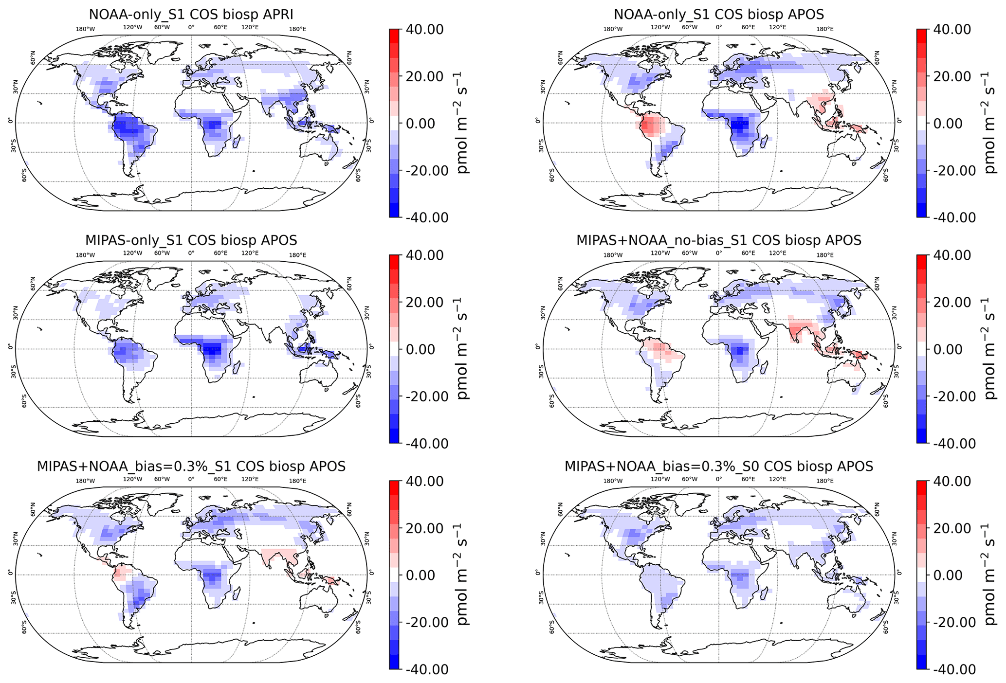
Figure 10The prior (APRI) and optimised (APOS) COS biosphere flux of all inversions. The flux represents the annual mean over 2009.
The prior COS budget is not in balance with a net excess sink of −432 GgS a−1, as described in Ma et al. (2021). The net fluxes of all inversion experiments are close to zero, which demonstrates the capability of the inverse model to close the gap in the global budget. All inversions reduce the biosphere uptake, albeit with different amounts depending on the inversion settings. Sometimes the biosphere sink even turns into a source, e.g. over Amazonia (Fig. S6 from inversion NOAA-only_S1). Although the MIPAS-only_S1 inversion overestimates COS both at the surface (Fig. 3) and in the lower troposphere (Fig. 8), the tropical biosphere remains a sink in this inversion (Fig. 10). When NOAA and MIPAS data are co-assimilated, the tropical biosphere still turns locally into a source but less strongly than for inversion NOAA-only_S1 (Fig. 10). From Table 5, it is clear that most of the error reduction is obtained for the biosphere flux. Ocean fluxes of both COS and CS2 only see marginal error reductions of a few percent at most. The error reduction on anthropogenic emissions is also small for the S1 inversions. However, as expected, error reductions become larger when their prior errors are increased from 10 % to 50 % in scenario S0. For instance, error reductions on the biomass burning emissions are increased from 0.4 % in scenario S1 to 31.0 % globally in scenario S0.
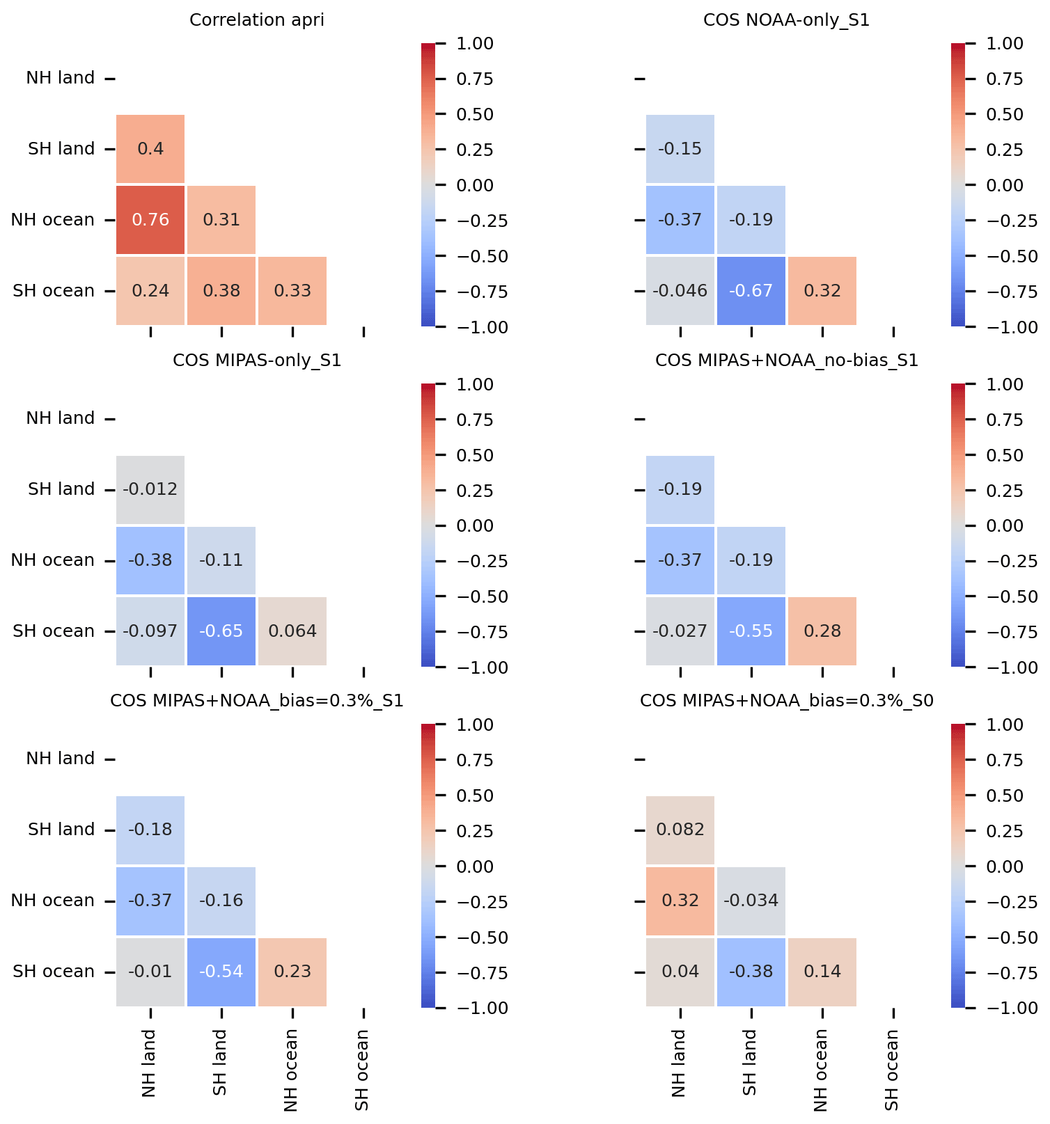
Figure 11Correlations of total COS fluxes between regions (NH lands and oceans, SH lands and oceans) for the prior and the inversions. The top-left panel is the prior correlation between regions. The total COS flux is the sum of anthropogenic, oceanic, biomass burning and biosphere fluxes.
In scenario S1, by far the largest adjustments are made to the tropical biosphere to close the COS budget. It is questionable, however, whether positive fluxes from Amazonia are realistic. In inversion MIPAS+NOAA_bias=0.3 %_S0, the biosphere remains a sink, as shown in Fig. 10. By reducing the prior error on the biosphere from 50 % to 10 %, the global biosphere prior error of 191.2 GgS a−1 in scenario S1 decreased to 38.2 GgS a−1 in scenario S0 (Table 5). To leverage the decrease in freedom, the biomass burning and anthropogenic errors were increased to 50 % in S0. Interestingly, despite the need for a tropical source, biomass burning emission showed a decrease from 126.6±27.5 to 95.8±18.9 GgS a−1 in scenario S0. This might imply that biomass burning is not responsible for the COS budget gap, in line with findings from Stinecipher et al. (2019). Instead, the budget is closed by increasing the anthropogenic CS2 and COS emissions and the CS2 ocean emissions. For instance, the global CS2 ocean source increased from 83.0±12.0 to 171.2±11.6 GgS a−1. Note that direct COS ocean emissions decreased in all scenarios (except for MIPAS-only_S1) because COS ocean exchange occurs mostly at high latitudes. Note also that many of the adjustments, especially in scenario S0, are large compared to the error settings. For instance, the global biosphere COS flux is adjusted from to GgS a−1. A similar large adjustment is seen for the oceanic CS2 emissions. This points to prior error settings that are too tight in scenario S0. However, the inversion system has to correct for the missing tropical source, which might be a structural model error (i.e. missing processes or incorrect regional or temporal correlation settings of sources and sinks). Adjusting the tropical fluxes outside the predefined prior error ranges is the only way to close the budget. In scenario S1 the error settings seem more realistic. However, as discussed above, the biosphere often turns into a source in the S1 scenario. These results underscore the importance of a proper quantification of the prior fluxes and their associated errors in inverse systems.
To investigate how well the different fluxes can be separated in our inversions, Fig. 11 shows posterior correlations of total COS fluxes aggregated over the different regions. In defining the fluxes, we quantified positive spatial and temporal correlations in the prior fluxes. After inversion, however, the correlations often turn strongly negative when the inversions cannot properly separate the fluxes. It can be inferred from Fig. 11 that the posterior fluxes from NH land and ocean are less (negatively) correlated than the fluxes from SH land and ocean. This implies that the inverse model can better separate NH land and ocean sources or sinks. This is because most NOAA surface observations are located in NH. The MIPAS-only_S1 and NOAA-only_S1 show high anti-correlations (−0.67 and −0.65) between SH land and ocean, which indicates poor separation of land and ocean fluxes. The cases MIPAS+NOAA_no-bias_S1 and MIPAS+NOAA_bias=0.3 %_S0 decrease the correlations between SH land and ocean to −0.55 and −0.38 respectively. This indicates that the inclusion of MIPAS data in the inversion leads to a better separation of land and ocean fluxes. Also, the prior error specification has a large impact on the posterior correlations. Specifically, the MIPAS+NOAA_bias=0.3 %_S0 inversion helps the separation of COS sources and sinks between land and ocean. The posterior CS2 correlations generally remain similar to the prior (see Fig. S7) because error reductions for CS2 fluxes are generally marginal, except in scenario S0 (MIPAS+NOAA_bias=0.3 %_S0).
Table 6The same as Table 5 but for Amazonia based on the 22 TransCom regions (Fig. 2 in Feng et al., 2011). Amazonia fluxes are calculated as the sum of South American Temperate and South American Tropical.
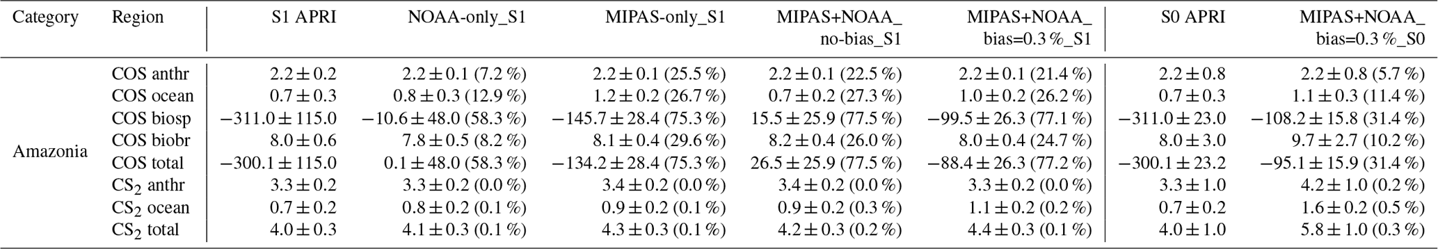
Table 6 summarises the COS and CS2 budgets, calculated for Amazonia. The Amazonia COS budgets are aggregated by adding the regions South American Temperate and South American Tropical of the 22 TransCom regions (Fig. 2 in Feng et al., 2011). The prior biosphere flux of Amazonia is −311.0 GgS a−1, and all the inversions tend to decrease the COS uptake by the biosphere, implying an overestimated prior biosphere sink or an unknown source over Amazonia. Notably, inversion NOAA-only_S1 obtained a posterior biosphere flux of GgS a−1. Interestingly, a fraction of northwestern Amazonia turned in a source (see Fig. 10) that may be questioned in light of the overestimated HIPPO 1 samples (Fig. 7). Inversion MIPAS-only_S1 obtained a larger posterior biosphere flux over Amazonia of −145.7 GgS a−1, which is, however, still less than half of the prior sink. When MIPAS and NOAA observations are co-assimilated, inversion MIPAS+NOAA_no-bias_S1 reverses the biosphere sink into a source of GgS a−1. The biosphere again remains a sink when bias correction is applied. Scenarios S1 and S0 with bias correction lead to a biosphere flux of and GgS a−1 respectively. Comparison to HIPPO 1 (Fig. 7) shows the smallest biases for scenario MIPAS+NOAA_bias=0.3 %_S0.
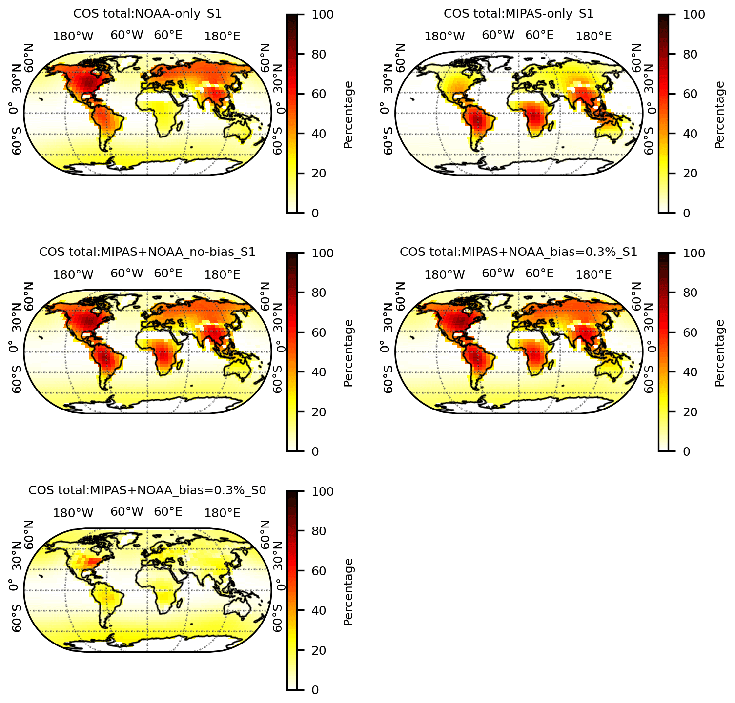
Figure 12Error reduction (in %) on the TM5 model grid scale for inversions as shown for the total COS flux. The total COS flux is the sum of anthropogenic, oceanic, biomass burning and biosphere fluxes.
4.5 Error reduction
In this section, maps of the error reduction are analysed. The error reduction on the grid scale of the model, aggregated over all direct COS fluxes, is shown in Fig. 12. For reference, the regional and global error reductions are shown in parentheses in Table 5. Inversion MIPAS-only_S1 mainly reduces the prior error over tropical regions, covering the Amazonia region, Africa and Central Asia. In contrast, inversion NOAA-only_S1 reduces the error mostly over the NH and mainly over North America, where the NOAA surface network is more dense. On the grid scale, the SH sees little error reduction, partly due to the lack of surface observational constraints but also because the ocean surface fluxes are distributed over a larger area compared to the biosphere fluxes. Inversions MIPAS+NOAA_no-bias_S1 and MIPAS+NOAA_bias=0.3 %_S1 reduce the errors again globally over the continents. This demonstrates the complementary effects of NOAA observations and MIPAS data on constraining the COS budget. Concerning error reductions for scenario S0, the error reduction is substantially smaller because the prior error on the biosphere flux is lowered from 50 % to 10 %. This largely limits the degrees of freedom to adjust the biosphere. It should be remembered that errors in our inverse system are defined as a percentage of the fluxes themselves. Biosphere fluxes are generally more localised and larger than ocean fluxes. As a result, the error reduction of the COS flux over the oceans is small compared to the error reduction of the land fluxes (see Fig. S8). Again, this points to the need to carefully construct the prior error covariance matrix B (Eq. 4). For instance, if we enlarge the prior errors on the CS2 ocean emissions to 150 % based on the S0 scenario (with a biosphere error of 10 %), we find that the CS2 ocean emissions are enlarged to provide the required tropical COS source (see scenario of SCS2X in Fig. S9). In that solution, we find comparable agreement to independent data with a global biosphere flux of ( GgS a−1 over Amazonia). Although the scenario is extreme (i.e. small freedom to adjust the tropical biosphere flux and large freedom to adjust the ocean CS2 flux), this inversion shows the need for accurate prior fluxes, including realistic errors.
The error reduction in the CS2 total flux (Fig. S10) is significantly smaller compared to COS (Fig. 12). Again, this is attributed to the small prior errors shown in Fig. S11. In scenario S0, in which the prior error on CS2 anthropogenic emissions is increased to 50 %, larger error reductions are seen over land, e.g. close to 30 % over NH land areas. Interestingly, the CS2 ocean fluxes roughly double in inversion S0, however, with only a small error reduction. This is clearly driven by the need for a tropical COS source and by the limited ability in scenario S0 to adjust the biosphere. It therefore seems logical to increase the prior errors on ocean CS2 emissions in future inversions.
A general feature of inversion results is that the tropical biosphere uptake is reduced, depending on the inversion settings. Recently, Stinecipher et al. (2022) reported that a smaller COS biosphere sink of −81.1±28.1 GgS a−1 over Amazonia (i.e. a low GPP model) leads to the best agreement to MIPAS observations, which is consistent with our findings. However, many of our inversions turn parts of Amazonia into a net source, and we question the realism of this result. This can potentially be the case that biosphere uptake is overestimated or that emissions from anthropogenic or biomass burning are underestimated. Indeed, we show biases when we compare simulations using our optimised fluxes to HIPPO 1 observations (Fig. 7), which disappear in a scenario in which we reduce the freedom to adjust the biosphere. This underscores the need to better characterise the prior fluxes, including their error settings. Our scenario S0 currently optimises fluxes well outside of the prior error settings. Specifically, a good balance should be found in optimising the tropical fluxes from land and ocean. The major challenge of inversions is how to improve the separation of ocean and land fluxes. The extra inversion SCS2X in Fig. S9 show that the SCS2X leads to a better separation of ocean and land fluxes. In SCS2X the prior errors of the ocean fluxes are increased to 150 %, and the prior errors of the biosphere fluxes are reduced to 10 %. On the positive side, we do find a similar result to Stinecipher et al. (2022), who also found a largely reduced GPP flux based on the COS proxy approach using MIPAS satellite data as climatological constraints. There was COS biosphere flux over the Amazon on a monthly timescale in 2008–2010. When the spin-up and spin-down periods are removed, results are consistent across the inversions. To further improve the robustness of the source attribution, it would be necessary to extend the time span of the inversions in future work. Adjustments of the budget terms outside of the prior errors could also point to structural model errors, such as unaccounted processes. For instance, enhanced production of COS from DMS oxidation through the intermediate HPMTF as recently reported (e.g. Jernigan et al., 2022) could be such a process. The difficulty of our inverse system to properly fit observations over remote oceans (e.g. SMO and MLO; Fig. 3) might be indicative of unresolved processes over the oceans. The enhanced CS2 flux could also come from DMS. Note that, given the chemical mechanism of DMS oxidation, any COS from DMS enhancement would not scale with the current prior flux because, in some regions with large DMS emissions, the atmospheric conditions almost exclude any COS production, while in other regions (e.g. the tropical Pacific) the chemical conditions tend to favour COS production.
One of the limitations of the assimilation of MIPAS data in this work is that we only used one specific level of MIPAS data to constrain the tropospheric COS mole fractions. We could exploit the MIPAS data more, e.g. by assimilating other levels. However, at higher latitudes the averaging kernels of MIPAS level 9 already mix information from the stratosphere (Fig. 2), which makes the comparison vulnerable to model errors associated with transport and stratospheric removal. At lower latitudes, there are much fewer useful observations after data quality control, especially missing observations over the tropics. A recent paper exploited TES data to analyse the seasonal cycle of COS over Amazonia (Wang et al., 2023). Assimilation of TES data, for instance in combination with MIPAS data, could be a possibility to further constrain the tropical COS budget. Unfortunately, like MIPAS, the TES instrument is no longer operational. Thus, more COS observations to better characterise COS concentrations and fluxes are still urgently needed.
In this study we have implemented the combined data assimilation of surface observations and MIPAS satellite data within the TM5-4DVAR system. The major conclusions are summarised as follows:
-
2008–2010 inversions show generally good agreement with both NOAA observations and MIPAS data, particularly with the assistance of a bias correction scheme. The optimised bias parameters show that the bias correction reduced MIPAS COS data at higher latitudes.
-
In all inversions, the largest adjustments are made to the biosphere fluxes. As a result, the required tropical COS source is obtained by strongly reducing the tropical biosphere, e.g. over Amazonia. Although the large flux adjustments over Amazonia are not always consistent with independent HIPPO observations, a yearly Amazonia COS uptake of 100 GgS is much smaller than the SiB4-based prior flux of about −300 GgS a−1 and is consistent with findings of a recent study by Stinecipher et al. (2022).
-
Analysis of the correlations between land and ocean fluxes indicates that assimilation of MIPAS data improves the separation between ocean sources and land sinks. Analysis of the error reduction shows that MIPAS data generally add information compared to a NOAA-only inversion.
-
A scenario in which the prior biosphere errors are reduced (S0) leads to a more realistic solution of the inverse problem. However, in this scenario, other fluxes are often optimised outside of the error settings. This could point to missing COS production terms in the model (e.g. from DMS) but also underscores the need to carefully construct the prior error covariance matrix B (Eq. 4).
Overall, our study shows that, although MIPAS data provide useful additional information, closure of the COS budget remains to some extent unresolved. Additional information could come from assimilation of satellite data from TES, ACE-FTS and IASI and of data from NDACC (Hannigan et al., 2022). On top of that, additional characterisation of the different COS sources (e.g. from oceans and DMS oxidation) and sinks (e.g. soils and biosphere) is recommended.
Codes of TM5-4DVAR are available on the website https://sourceforge.net/projects/tm5/ (TM5-4DVAR team, 2024). Codes developed for generating the results of this study can be provided by the corresponding author upon reasonable request.
MIPAS satellite COS measurements are available at https://earth.esa.int/eogateway/instruments/mipas (MIPAS, 2024). NOAA surface measurement of COS is available at https://www.esrl.noaa.gov/gmd/dv/data/ (NOAA Global Monitoring Laboratory, 2024). HIPPO COS observations are available at https://www.eol.ucar.edu/field_projects/hippo (HIPPO, 2024).
The supplement related to this article is available online at: https://doi.org/10.5194/acp-24-6047-2024-supplement.
JM and MCK designed the study and implemented the algorithms. JM performed numerical experiments and data analysis. TR and MvH gave valuable discussions and inputs on this work. LMJK provided SiB4 biosphere flux for model input. NG provided MIPAS data and helpful discussions on usage of MIPAS data. SAM provided the NOAA surface network. JM and MCK wrote the paper with comments from all co-authors.
At least one of the (co-)authors is a member of the editorial board of Atmospheric Chemistry and Physics. The peer-review process was guided by an independent editor, and the authors also have no other competing interests to declare.
Publisher’s note: Copernicus Publications remains neutral with regard to jurisdictional claims made in the text, published maps, institutional affiliations, or any other geographical representation in this paper. While Copernicus Publications makes every effort to include appropriate place names, the final responsibility lies with the authors.
This work is carried out on the Dutch National Supercomputer Infrastructure with the support from SURFsara and Snellius. The authors acknowledge Michael Kiefer at KIT for the MIPAS data product and Lei Hu at the NOAA Global Monitoring Laboratory for NOAA airborne platform measurements. The authors acknowledge the NOAA team for providing the NOAA surface data and maintenance of the data.
This research has been supported by the EU HORIZON European Research Council (grant no. 742798).
This paper was edited by Jason West and reviewed by two anonymous referees.
Abadie, C., Maignan, F., Remaud, M., Ogée, J., Campbell, J. E., Whelan, M. E., Kitz, F., Spielmann, F. M., Wohlfahrt, G., Wehr, R., Sun, W., Raoult, N., Seibt, U., Hauglustaine, D., Lennartz, S. T., Belviso, S., Montagne, D., and Peylin, P.: Global modelling of soil carbonyl sulfide exchanges, Biogeosciences, 19, 2427–2463, https://doi.org/10.5194/bg-19-2427-2022, 2022. a, b
Baartman, S. L., Krol, M. C., Röckmann, T., Hattori, S., Kamezaki, K., Yoshida, N., and Popa, M. E.: A GC-IRMS method for measuring sulfur isotope ratios of carbonyl sulfide from small air samples, Open Research Europe, 1, 105, https://doi.org/10.12688/openreseurope.13875.2, 2021. a
Barkley, M. P., Palmer, P. I., Boone, C. D., Bernath, P. F., and Suntharalingam, P.: Global distributions of carbonyl sulfide in the upper troposphere and stratosphere, Geophys. Res. Lett., 35, L14810, https://doi.org/10.1029/2008GL034270, 2008. a
Barnes, I., Becker, K. H., and Patroescu, I.: The tropospheric oxidation of DMS: A new source of OCS, Geophys. Res. Lett., 21, 2389–2392, https://doi.org/10.1029/94GL02499, 1994. a, b
Basu, S., Guerlet, S., Butz, A., Houweling, S., Hasekamp, O., Aben, I., Krummel, P., Steele, P., Langenfelds, R., Torn, M., Biraud, S., Stephens, B., Andrews, A., and Worthy, D.: Global CO2 fluxes estimated from GOSAT retrievals of total column CO2, Atmos. Chem. Phys., 13, 8695–8717, https://doi.org/10.5194/acp-13-8695-2013, 2013. a
Bergamaschi, P., Krol, M., Meirink, J. F., Dentener, F., Segers, A., Van Aardenne, J., Monni, S., Vermeulen, A. T., Schmidt, M., Ramonet, M., Yver, C., Meinhardt, F., Nisbet, E. G., Fisher, R. E., O'Doherty, S., and Dlugokencky, E. J.: Inverse modeling of European CH4 emissions 2001–2006, J. Geophys. Res.-Atmos., 115, D22309, https://doi.org/10.1029/2010JD014180, 2010. a
Bernath, P., Crouse, J., Hughes, R., and Boone, C.: The Atmospheric Chemistry Experiment Fourier transform spectrometer (ACE-FTS) version 4.1 retrievals: Trends and seasonal distributions, J. Quant. Spectrosc. Ra., 259, 107409, https://doi.org/10.1016/j.jqsrt.2020.107409, 2021. a
Berry, J., Wolf, A., Campbell, J. E., Baker, I., Blake, N., Blake, D., Denning, A. S., Kawa, S. R., Montzka, S. A., Seibt, U., Stimler, K., Yakir, D., and Zhu, Z.: A coupled model of the global cycles of carbonyl sulfide and CO2: A possible new window on the carbon cycle, J. Geophys. Res.-Biogeo., 118, 842–852, 2013. a, b, c, d, e, f
Brasseur, G. P. and Jacob, D. J.: Inverse Modeling for Atmospheric Chemistry, in: Modeling of Atmospheric Chemistry, Cambridge University Press, https://doi.org/10.1017/9781316544754.012, 2017. a, b
Brühl, C., Lelieveld, J., Crutzen, P. J., and Tost, H.: The role of carbonyl sulphide as a source of stratospheric sulphate aerosol and its impact on climate, Atmos. Chem. Phys., 12, 1239–1253, https://doi.org/10.5194/acp-12-1239-2012, 2012. a, b
Campbell, J., Whelan, M., Seibt, U., Smith, S. J., Berry, J., and Hilton, T. W.: Atmospheric carbonyl sulfide sources from anthropogenic activity: Implications for carbon cycle constraints, Geophys. Res. Lett., 42, 3004–3010, 2015. a
Campbell, J., Berry, J., Seibt, U., Smith, S. J., Montzka, S., Launois, T., Belviso, S., Bopp, L., and Laine, M.: Large historical growth in global terrestrial gross primary production, Nature, 544, 84–87, 2017. a
Campbell, J. E., Carmichael, G. R., Chai, T., Mena-Carrasco, M., Tang, Y., Blake, D., Blake, N., Vay, S. A., Collatz, G. J., Baker, I., Berry, J. A., Montzka, S. A., Sweeney, C., Schnoor, J. L., and Stanier, C. O.: Photosynthetic control of atmospheric carbonyl sulfide during the growing season, Science, 322, 1085–1088, 2008. a, b, c
Camy-Peyret, C., Liuzzi, G., Masiello, G., Serio, C., Venafra, S., and Montzka, S.: Assessment of IASI capability for retrieving carbonyl sulphide (OCS), J. Quant. Spectrosc. Ra., 201, 197–208, 2017. a
Cartwright, M. P., Harrison, J. J., and Moore, D. P.: Retrievals of Atmospheric Carbonyl Sulfide from IASI, vEGU21, the 23rd EGU General Assembly, online, 19–30 April, 2021, EGU21–10373, https://doi.org/10.5194/egusphere-egu21-10373, 2021. a
Cartwright, M. P., Pope, R. J., Harrison, J. J., Chipperfield, M. P., Wilson, C., Feng, W., Moore, D. P., and Suntharalingam, P.: Constraining the budget of atmospheric carbonyl sulfide using a 3-D chemical transport model, Atmos. Chem. Phys., 23, 10035–10056, https://doi.org/10.5194/acp-23-10035-2023, 2023. a
Cheng, B.-M. and Lee, Y.-P.: Rate constant of OH+ OCS reaction over the temperature range 255–483 K, Int. J. Chem. Kinet., 18, 1303–1314, 1986. a
Chin, M. and Davis, D.: Global sources and sinks of OCS and CS2 and their distributions, Global Biogeochem. Cy., 7, 321–337, 1993. a
Commane, R., Meredith, L. K., Baker, I. T., Berry, J. A., Munger, J. W., Montzka, S. A., Templer, P. H., Juice, S. M., Zahniser, M. S., and Wofsy, S. C.: Seasonal fluxes of carbonyl sulfide in a midlatitude forest, P. Natl. Acad. Sci. USA, 112, 14162–14167, 2015. a
Crutzen, P. J.: The possible importance of CSO for the sulfate layer of the stratosphere, Geophys. Res. Lett., 3, 73–76, https://doi.org/10.1029/GL003i002p00073, 1976. a
Davidson, C., Amrani, A., and Angert, A.: Tropospheric carbonyl sulfide mass balance based on direct measurements of sulfur isotopes, P. Natl. Acad. Sci. USA, 118, e2020060118, https://doi.org/10.1073/pnas.2020060118, 2021. a
Dee, D. P., Uppala, S. M., Simmons, A. J., Berrisford, P., Poli, P., Kobayashi, S., Andrae, U., Balmaseda, M. A., Balsamo, G., Bauer, P., Bechtold, P., Beljaars, A. C. M., van de Berg, L., Bidlot, J., Bormann, N., Delsol, C., Dragani, R., Fuentes, M., Geer, A. J., Haimberger, L., Healy, S. B., Hersbach, H., Hólm, E. V., Isaksen, L., Kållberg, P., Köhler, M., Matricardi, M., McNally, A. P., Monge-Sanz, B. M., Morcrette, J.-J., Park, B.-K., Peubey, C., de Rosnay, P., Tavolato, C., Thépaut, J.-N., and Vitart, F.: The ERA-Interim reanalysis: Configuration and performance of the data assimilation system, Q. J. Roy. Meteor. Soc., 137, 553–597, 2011. a
Du, Q., Zhang, C., Mu, Y., Cheng, Y., Zhang, Y., Liu, C., Song, M., Tian, D., Liu, P., Liu, J., Xue, C., and Ye, C.: An important missing source of atmospheric carbonyl sulfide: Domestic coal combustion, Geophys. Res. Lett., 43, 8720–8727, https://doi.org/10.1002/2016GL070075, 2016. a
Feng, L., Palmer, P. I., Yang, Y., Yantosca, R. M., Kawa, S. R., Paris, J.-D., Matsueda, H., and Machida, T.: Evaluating a 3-D transport model of atmospheric CO2 using ground-based, aircraft, and space-borne data, Atmos. Chem. Phys., 11, 2789–2803, https://doi.org/10.5194/acp-11-2789-2011, 2011. a, b
Fischer, H., Birk, M., Blom, C., Carli, B., Carlotti, M., von Clarmann, T., Delbouille, L., Dudhia, A., Ehhalt, D., Endemann, M., Flaud, J. M., Gessner, R., Kleinert, A., Koopman, R., Langen, J., López-Puertas, M., Mosner, P., Nett, H., Oelhaf, H., Perron, G., Remedios, J., Ridolfi, M., Stiller, G., and Zander, R.: MIPAS: an instrument for atmospheric and climate research, Atmos. Chem. Phys., 8, 2151–2188, https://doi.org/10.5194/acp-8-2151-2008, 2008. a
Friedlingstein, P., O'Sullivan, M., Jones, M. W., Andrew, R. M., Hauck, J., Olsen, A., Peters, G. P., Peters, W., Pongratz, J., Sitch, S., Le Quéré, C., Canadell, J. G., Ciais, P., Jackson, R. B., Alin, S., Aragão, L. E. O. C., Arneth, A., Arora, V., Bates, N. R., Becker, M., Benoit-Cattin, A., Bittig, H. C., Bopp, L., Bultan, S., Chandra, N., Chevallier, F., Chini, L. P., Evans, W., Florentie, L., Forster, P. M., Gasser, T., Gehlen, M., Gilfillan, D., Gkritzalis, T., Gregor, L., Gruber, N., Harris, I., Hartung, K., Haverd, V., Houghton, R. A., Ilyina, T., Jain, A. K., Joetzjer, E., Kadono, K., Kato, E., Kitidis, V., Korsbakken, J. I., Landschützer, P., Lefèvre, N., Lenton, A., Lienert, S., Liu, Z., Lombardozzi, D., Marland, G., Metzl, N., Munro, D. R., Nabel, J. E. M. S., Nakaoka, S.-I., Niwa, Y., O'Brien, K., Ono, T., Palmer, P. I., Pierrot, D., Poulter, B., Resplandy, L., Robertson, E., Rödenbeck, C., Schwinger, J., Séférian, R., Skjelvan, I., Smith, A. J. P., Sutton, A. J., Tanhua, T., Tans, P. P., Tian, H., Tilbrook, B., van der Werf, G., Vuichard, N., Walker, A. P., Wanninkhof, R., Watson, A. J., Willis, D., Wiltshire, A. J., Yuan, W., Yue, X., and Zaehle, S.: Global Carbon Budget 2020, Earth Syst. Sci. Data, 12, 3269–3340, https://doi.org/10.5194/essd-12-3269-2020, 2020. a
Friedlingstein, P., Jones, M. W., O'Sullivan, M., Andrew, R. M., Bakker, D. C. E., Hauck, J., Le Quéré, C., Peters, G. P., Peters, W., Pongratz, J., Sitch, S., Canadell, J. G., Ciais, P., Jackson, R. B., Alin, S. R., Anthoni, P., Bates, N. R., Becker, M., Bellouin, N., Bopp, L., Chau, T. T. T., Chevallier, F., Chini, L. P., Cronin, M., Currie, K. I., Decharme, B., Djeutchouang, L. M., Dou, X., Evans, W., Feely, R. A., Feng, L., Gasser, T., Gilfillan, D., Gkritzalis, T., Grassi, G., Gregor, L., Gruber, N., Gürses, Ö., Harris, I., Houghton, R. A., Hurtt, G. C., Iida, Y., Ilyina, T., Luijkx, I. T., Jain, A., Jones, S. D., Kato, E., Kennedy, D., Klein Goldewijk, K., Knauer, J., Korsbakken, J. I., Körtzinger, A., Landschützer, P., Lauvset, S. K., Lefèvre, N., Lienert, S., Liu, J., Marland, G., McGuire, P. C., Melton, J. R., Munro, D. R., Nabel, J. E. M. S., Nakaoka, S.-I., Niwa, Y., Ono, T., Pierrot, D., Poulter, B., Rehder, G., Resplandy, L., Robertson, E., Rödenbeck, C., Rosan, T. M., Schwinger, J., Schwingshackl, C., Séférian, R., Sutton, A. J., Sweeney, C., Tanhua, T., Tans, P. P., Tian, H., Tilbrook, B., Tubiello, F., van der Werf, G. R., Vuichard, N., Wada, C., Wanninkhof, R., Watson, A. J., Willis, D., Wiltshire, A. J., Yuan, W., Yue, C., Yue, X., Zaehle, S., and Zeng, J.: Global Carbon Budget 2021, Earth Syst. Sci. Data, 14, 1917–2005, https://doi.org/10.5194/essd-14-1917-2022, 2022a. a
Friedlingstein, P., O'Sullivan, M., Jones, M. W., Andrew, R. M., Gregor, L., Hauck, J., Le Quéré, C., Luijkx, I. T., Olsen, A., Peters, G. P., Peters, W., Pongratz, J., Schwingshackl, C., Sitch, S., Canadell, J. G., Ciais, P., Jackson, R. B., Alin, S. R., Alkama, R., Arneth, A., Arora, V. K., Bates, N. R., Becker, M., Bellouin, N., Bittig, H. C., Bopp, L., Chevallier, F., Chini, L. P., Cronin, M., Evans, W., Falk, S., Feely, R. A., Gasser, T., Gehlen, M., Gkritzalis, T., Gloege, L., Grassi, G., Gruber, N., Gürses, Ö., Harris, I., Hefner, M., Houghton, R. A., Hurtt, G. C., Iida, Y., Ilyina, T., Jain, A. K., Jersild, A., Kadono, K., Kato, E., Kennedy, D., Klein Goldewijk, K., Knauer, J., Korsbakken, J. I., Landschützer, P., Lefèvre, N., Lindsay, K., Liu, J., Liu, Z., Marland, G., Mayot, N., McGrath, M. J., Metzl, N., Monacci, N. M., Munro, D. R., Nakaoka, S.-I., Niwa, Y., O'Brien, K., Ono, T., Palmer, P. I., Pan, N., Pierrot, D., Pocock, K., Poulter, B., Resplandy, L., Robertson, E., Rödenbeck, C., Rodriguez, C., Rosan, T. M., Schwinger, J., Séférian, R., Shutler, J. D., Skjelvan, I., Steinhoff, T., Sun, Q., Sutton, A. J., Sweeney, C., Takao, S., Tanhua, T., Tans, P. P., Tian, X., Tian, H., Tilbrook, B., Tsujino, H., Tubiello, F., van der Werf, G. R., Walker, A. P., Wanninkhof, R., Whitehead, C., Willstrand Wranne, A., Wright, R., Yuan, W., Yue, C., Yue, X., Zaehle, S., Zeng, J., and Zheng, B.: Global Carbon Budget 2022, Earth Syst. Sci. Data, 14, 4811–4900, https://doi.org/10.5194/essd-14-4811-2022, 2022b. a
Fung, K. M., Heald, C. L., Kroll, J. H., Wang, S., Jo, D. S., Gettelman, A., Lu, Z., Liu, X., Zaveri, R. A., Apel, E. C., Blake, D. R., Jimenez, J.-L., Campuzano-Jost, P., Veres, P. R., Bates, T. S., Shilling, J. E., and Zawadowicz, M.: Exploring dimethyl sulfide (DMS) oxidation and implications for global aerosol radiative forcing, Atmos. Chem. Phys., 22, 1549–1573, https://doi.org/10.5194/acp-22-1549-2022, 2022. a, b
Glatthor, N., Höpfner, M., Baker, I. T., Berry, J., Campbell, J., Kawa, S. R., Krysztofiak, G., Leyser, A., Sinnhuber, B.-M., Stiller, G., Stinecipher, J., and von Clarmann, T.: Tropical sources and sinks of carbonyl sulfide observed from space, Geophys. Res. Lett., 42, 10–082, 2015. a, b
Glatthor, N., Höpfner, M., Leyser, A., Stiller, G. P., von Clarmann, T., Grabowski, U., Kellmann, S., Linden, A., Sinnhuber, B.-M., Krysztofiak, G., and Walker, K. A.: Global carbonyl sulfide (OCS) measured by MIPAS/Envisat during 2002–2012, Atmos. Chem. Phys., 17, 2631–2652, https://doi.org/10.5194/acp-17-2631-2017, 2017. a, b, c
Hannigan, J. W., Ortega, I., Shams, S. B., Blumenstock, T., Campbell, J. E., Conway, S., Flood, V., Garcia, O., Griffith, D., Grutter, M., Hase, F., Jeseck, P., Jones, N., Mahieu, E., Makarova, M., Mazière, M. D., Isamu, M., Murata, I., Nagahama, T., Nakijima, H., Notholt, J., Palm, M., Poberovskii, A., Rettinger, M., Robinson, J., Röhling, A. N., Schneider, M., Servais, C., Smale, D., Stremme, W., Strong, K., Sussmann, R., Te, Y., Vigouroux, C., and Wizenberg, T.: Global atmospheric OCS trend analysis from 22 NDACC stations, J. Geophys. Res.-Atmos., 127, e2021JD035764, https://doi.org/10.1029/2021JD035764, 2022. a, b, c
Hattori, S., Kamezaki, K., and Yoshida, N.: Constraining the atmospheric OCS budget from sulfur isotopes, P. Natl. Acad. Sci. USA, 117, 20447–20452, 2020. a
HIPPO: HIPPO Data, https://www.eol.ucar.edu/field_projects/hippo, last access: 22 May 2024. a
Houweling, S., Krol, M., Bergamaschi, P., Frankenberg, C., Dlugokencky, E. J., Morino, I., Notholt, J., Sherlock, V., Wunch, D., Beck, V., Gerbig, C., Chen, H., Kort, E. A., Röckmann, T., and Aben, I.: A multi-year methane inversion using SCIAMACHY, accounting for systematic errors using TCCON measurements, Atmos. Chem. Phys., 14, 3991–4012, https://doi.org/10.5194/acp-14-3991-2014, 2014. a, b
Hu, L., Montzka, S. A., Kaushik, A., Andrews, A. E., Sweeney, C., Miller, J., Baker, I. T., Denning, S., Campbell, E., Shiga, Y. P., Tans P., Siso M. C., Crotwell, M., McKain, K., Thoning, K., Hall, B., Vimont, I., Elkins, J. W., Whelan, M. E., and Suntharalingamg, P.: COS-derived GPP relationships with temperature and light help explain high-latitude atmospheric CO2 seasonal cycle amplification, P. Natl. Acad. Sci. USA, 118, e2103423118, https://doi.org/10.1073/pnas.2103423118, 2021. a
Jernigan, C. M., Fite, C. H., Vereecken, L., Berkelhammer, M. B., Rollins, A. W., Rickly, P. S., Novelli, A., Taraborrelli, D., Holmes, C. D., and Bertram, T. H.: Efficient Production of Carbonyl Sulfide in the Low-NOx Oxidation of Dimethyl Sulfide, Geophys. Res. Lett., 49, e2021GL096838, https://doi.org/10.1029/2021GL096838, 2022. a, b, c, d
Kettle, A., Kuhn, U., von Hobe, M. V., Kesselmeier, J., and Andreae, M.: Global budget of atmospheric carbonyl sulfide: Temporal and spatial variations of the dominant sources and sinks, J. Geophys. Res.-Atmos., 107, 4658, https://doi.org/10.1029/2002JD002187, 2002. a, b, c, d, e, f
Khan, M. A., Gillespie, S. M., Razis, B., Xiao, P., Davies-Coleman, M. T., Percival, C. J., Derwent, R. G., Dyke, J. M., Ghosh, M. V., Lee, E. P., and Shallcross, D. E.: A modelling study of the atmospheric chemistry of DMS using the global model, STOCHEM-CRI, Atmos. Environ., 127, 69–79, https://doi.org/10.1016/j.atmosenv.2015.12.028, 2016. a
Kooijmans, L. M. J., Maseyk, K., Seibt, U., Sun, W., Vesala, T., Mammarella, I., Kolari, P., Aalto, J., Franchin, A., Vecchi, R., Valli, G., and Chen, H.: Canopy uptake dominates nighttime carbonyl sulfide fluxes in a boreal forest, Atmos. Chem. Phys., 17, 11453–11465, https://doi.org/10.5194/acp-17-11453-2017, 2017. a
Kooijmans, L. M. J., Sun, W., Aalto, J., Erkkilä, K.-M. M., Maseyk, K., Seibt, U., Vesala, T., Mammarella, I., and Chen, H.: Influences of light and humidity on carbonyl sulfide-based estimates of photosynthesis, P. Natl. Acad. Sci. USA, 116, 2470–2475, https://doi.org/10.1073/pnas.1807600116, 2019. a
Kooijmans, L. M. J., Cho, A., Ma, J., Kaushik, A., Haynes, K. D., Baker, I., Luijkx, I. T., Groenink, M., Peters, W., Miller, J. B., Berry, J. A., Ogée, J., Meredith, L. K., Sun, W., Kohonen, K.-M., Vesala, T., Mammarella, I., Chen, H., Spielmann, F. M., Wohlfahrt, G., Berkelhammer, M., Whelan, M. E., Maseyk, K., Seibt, U., Commane, R., Wehr, R., and Krol, M.: Evaluation of carbonyl sulfide biosphere exchange in the Simple Biosphere Model (SiB4), Biogeosciences, 18, 6547–6565, https://doi.org/10.5194/bg-18-6547-2021, 2021. a, b, c, d
Koren, G.: Constraining photosynthesis with Δ17O in CO2, Nat. Rev. Earth Environ., 2, 744–744, 2021. a
Kremser, S., Thomason, L. W., von Hobe, M., Hermann, M., Deshler, T., Timmreck, C., Toohey, M., Stenke, A., Schwarz, J. P., Weigel, R., Fueglistaler, S., Prata, F. J., Vernier, J. P., Schlager, H., Barnes, J. E., Antuña-Marrero, J. C., Fairlie, D., Palm, M., Mahieu, E., Notholt, J., Rex, M., Bingen, C., Vanhellemont, F., Bourassa, A., Plane, J. M., Klocke, D., Carn, S. A., Clarisse, L., Trickl, T., Neely, R., James, A. D., Rieger, L., Wilson, J. C., and Meland, B.: Stratospheric aerosol–Observations, processes, and impact on climate, Rev. Geophys., 54, 278–335, https://doi.org/10.1002/2015RG000511, 2016. a
Krol, M., Houweling, S., Bregman, B., van den Broek, M., Segers, A., van Velthoven, P., Peters, W., Dentener, F., and Bergamaschi, P.: The two-way nested global chemistry-transport zoom model TM5: algorithm and applications, Atmos. Chem. Phys., 5, 417–432, https://doi.org/10.5194/acp-5-417-2005, 2005. a, b
Krol, M. C., Meirink, J. F., Bergamaschi, P., Mak, J. E., Lowe, D., Jöckel, P., Houweling, S., and Röckmann, T.: What can 14CO measurements tell us about OH?, Atmos. Chem. Phys., 8, 5033–5044, https://doi.org/10.5194/acp-8-5033-2008, 2008. a
Krysztofiak, G., Té, Y. V., Catoire, V., Berthet, G., Toon, G. C., Jégou, F., Jeseck, P., and Robert, C.: Carbonyl sulphide (OCS) variability with latitude in the atmosphere, Atmos. Ocean, 53, 89–101, https://doi.org/10.1080/07055900.2013.876609, 2015. a
Kuai, L., Worden, J., Kulawik, S. S., Montzka, S. A., and Liu, J.: Characterization of Aura TES carbonyl sulfide retrievals over ocean, Atmos. Meas. Tech., 7, 163–172, https://doi.org/10.5194/amt-7-163-2014, 2014. a
Kuai, L., Worden, J. R., Campbell, J. E., Kulawik, S. S., Li, K.-F., Lee, M., Weidner, R. J., Montzka, S. A., Moore, F. L., Berry, J. A., Baker, I., Denning, A. S., Bian, H., Bowman, K. W., Liu, J., and Yung, Y. L.: Estimate of carbonyl sulfide tropical oceanic surface fluxes using Aura Tropospheric Emission Spectrometer observations, J. Geophys. Res.-Atmos., 120, 11012–11023, https://doi.org/10.1002/2015JD023493, 2015. a, b, c
Lana, A., Bell, T., Simó, R., Vallina, S., Ballabrera-Poy, J., Kettle, A., Dachs, J., Bopp, L., Saltzman, E., Stefels, J., Johnson, J. E., and Liss, P. S.: An updated climatology of surface dimethlysulfide concentrations and emission fluxes in the global ocean, Global Biogeochem. Cy., 25, GB1004, https://doi.org/10.1029/2010GB003850, 2011. a
Lanczos, C.: An iteration method for the solution of the eigenvalue problem of linear differential and integral operators, J. Res. Nat. Bur. Stand., 45, 255, https://doi.org/10.6028/jres.045.026, 1950. a
Lee, C.-L. and Brimblecombe, P.: Anthropogenic contributions to global carbonyl sulfide, carbon disulfide and organosulfides fluxes, Earth-Sci. Rev., 160, 1–18, 2016. a
Lennartz, S. T., Marandino, C. A., von Hobe, M., Cortes, P., Quack, B., Simo, R., Booge, D., Pozzer, A., Steinhoff, T., Arevalo-Martinez, D. L., Kloss, C., Bracher, A., Röttgers, R., Atlas, E., and Krüger, K.: Direct oceanic emissions unlikely to account for the missing source of atmospheric carbonyl sulfide, Atmos. Chem. Phys., 17, 385–402, https://doi.org/10.5194/acp-17-385-2017, 2017. a
Lennartz, S. T., Marandino, C. A., von Hobe, M., Andreae, M. O., Aranami, K., Atlas, E., Berkelhammer, M., Bingemer, H., Booge, D., Cutter, G., Cortes, P., Kremser, S., Law, C. S., Marriner, A., Simó, R., Quack, B., Uher, G., Xie, H., and Xu, X.: Marine carbonyl sulfide (OCS) and carbon disulfide (CS2): a compilation of measurements in seawater and the marine boundary layer, Earth Syst. Sci. Data, 12, 591–609, https://doi.org/10.5194/essd-12-591-2020, 2020. a
Lennartz, S. T., Gauss, M., von Hobe, M., and Marandino, C. A.: Monthly resolved modelled oceanic emissions of carbonyl sulphide and carbon disulphide for the period 2000–2019, Earth Syst. Sci. Data, 13, 2095–2110, https://doi.org/10.5194/essd-13-2095-2021, 2021. a
Ma, J., Kooijmans, L. M. J., Cho, A., Montzka, S. A., Glatthor, N., Worden, J. R., Kuai, L., Atlas, E. L., and Krol, M. C.: Inverse modelling of carbonyl sulfide: implementation, evaluation and implications for the global budget, Atmos. Chem. Phys., 21, 3507–3529, https://doi.org/10.5194/acp-21-3507-2021, 2021. a, b, c, d, e, f, g, h, i, j, k, l, m, n, o, p, q, r, s, t, u
Maignan, F., Abadie, C., Remaud, M., Kooijmans, L. M. J., Kohonen, K.-M., Commane, R., Wehr, R., Campbell, J. E., Belviso, S., Montzka, S. A., Raoult, N., Seibt, U., Shiga, Y. P., Vuichard, N., Whelan, M. E., and Peylin, P.: Carbonyl sulfide: comparing a mechanistic representation of the vegetation uptake in a land surface model and the leaf relative uptake approach, Biogeosciences, 18, 2917–2955, https://doi.org/10.5194/bg-18-2917-2021, 2021. a
Meirink, J. F., Bergamaschi, P., and Krol, M. C.: Four-dimensional variational data assimilation for inverse modelling of atmospheric methane emissions: method and comparison with synthesis inversion, Atmos. Chem. Phys., 8, 6341–6353, https://doi.org/10.5194/acp-8-6341-2008, 2008. a, b, c, d
MIPAS: MIPAS Data, https://earth.esa.int/eogateway/instruments/mipas, last access: 22 May 2024. a
Monteil, G., Houweling, S., Butz, A., Guerlet, S., Schepers, D., Hasekamp, O., Frankenberg, C., Scheepmaker, R., Aben, I., and Röckmann, T.: Comparison of CH4 inversions based on 15 months of GOSAT and SCIAMACHY observations, J. Geophys. Res.-Atmos., 118, 11807–11823, https://doi.org/10.1002/2013JD019760, 2013. a
Montzka, S., Calvert, P., Hall, B., Elkins, J., Conway, T., Tans, P., and Sweeney, C.: On the global distribution, seasonality, and budget of atmospheric carbonyl sulfide (COS) and some similarities to CO2, J. of Geophys. Res.-Atmos., 112, D09302, https://doi.org/10.1029/2006JD007665, 2007. a, b, c, d, e
Nagori, J., Nechita-Bândă, N., Oscar Danielache, S., Shinkai, M., Röckmann, T., and Krol, M.: Modelling the atmospheric 34S-sulfur budget in a column model under volcanically quiescent conditions, Atmos. Chem. Phys. Discuss. [preprint], https://doi.org/10.5194/acp-2022-68, 2022. a
NOAA Global Monitoring Laboratory: GML Data, https://www.esrl.noaa.gov/gmd/dv/data/, last access: 22 May 2024. a
Ogée, J., Sauze, J., Kesselmeier, J., Genty, B., Van Diest, H., Launois, T., and Wingate, L.: A new mechanistic framework to predict OCS fluxes from soils, Biogeosciences, 13, 2221–2240, https://doi.org/10.5194/bg-13-2221-2016, 2016. a
Remaud, M., Chevallier, F., Maignan, F., Belviso, S., Berchet, A., Parouffe, A., Abadie, C., Bacour, C., Lennartz, S., and Peylin, P.: Plant gross primary production, plant respiration and carbonyl sulfide emissions over the globe inferred by atmospheric inverse modelling, Atmos. Chem. Phys., 22, 2525–2552, https://doi.org/10.5194/acp-22-2525-2022, 2022. a, b, c, d
Spielmann, F., Wohlfahrt, G., Hammerle, A., Kitz, F., Migliavacca, M., Alberti, G., Ibrom, A., El-Madany, T. S., Gerdel, K., Moreno, G., Kolle O., Karl T., Peressotti, A., and Vedove, G. D.: Gross primary productivity of four European ecosystems constrained by joint CO2 and COS flux measurements, Geophys. Res. Lett., 46, 5284–5293, 2019. a
Spivakovsky, C. M., Logan, J. A., Montzka, S. A., Balkanski, Y. J., Foreman-Fowler, M., Jones, D. B., Horowitz, L. W., Fusco, A. C., Brenninkmeijer, C. A., Prather, M. J., Wofsy, S. C., and McElroy, M. B.: Three-dimensional climatological distribution of tropospheric OH: Update and evaluation, J. Geophys. Res., 105, 8931–8980, https://doi.org/10.1029/1999JD901006, 2000. a
Stickel, R. E., Chin, M., Daykin, E. P., Hynes, A. J., Wine, P. H., and Wallington, T. J.: Mechanistic studies of the oh-initiated oxidation of CS2 in the presence of O-2, J. Phys. Chem., 97, 13653–13661, 1993. a
Stimler, K., Montzka, S. A., Berry, J. A., Rudich, Y., and Yakir, D.: Relationships between carbonyl sulfide (COS) and CO2 during leaf gas exchange, New Phytol., 186, 869–878, 2010. a
Stinecipher, J. R., Cameron-Smith, P. J., Blake, N. J., Kuai, L., Lejeune, B., Mahieu, E., Simpson, I. J., and Campbell, J. E.: Biomass Burning Unlikely to Account for Missing Source of Carbonyl Sulfide, Geophys. Res. Lett., 46, 14912–14920, https://doi.org/10.1029/2019GL085567, 2019. a, b
Stinecipher, J. R., Cameron-Smith, P., Kuai, L., Glatthor, N., Höpfner, M., Baker, I., Beer, C., Bowman, K., Lee, M., Miller, S. M., Parazoo, N., and Campbell, J. E.: Remotely Sensed Carbonyl Sulfide Constrains Model Estimates of Amazon Primary Productivity, Geophys. Res. Lett., 49, e2021GL096802, https://doi.org/10.1029/2021GL096802, 2022. a, b, c, d, e, f
Suntharalingam, P., Kettle, A. J., Montzka, S. M., and Jacob, D. J.: Global 3-D model analysis of the seasonal cycle of atmospheric carbonyl sulfide: Implications for terrestrial vegetation uptake, Geophys. Res. Lett., 35, L19801, https://doi.org/10.1029/2008GL034332, 2008. a, b, c, d, e, f
Tarantola, A.: Inverse problem theory and methods for model parameter estimation, SIAM, 2005. a, b
TM5-4DVAR team: TM5-4DVAR, https://sourceforge.net/projects/tm5/, last access: 22 May 2024. a
Turco, R., Whitten, R., Toon, O., Pollack, J., and Hamill, P.: OCS, stratospheric aerosols and climate, Nature, 283, 283–285, 1980. a
Veres, P. R., Neuman, J. A., Bertram, T. H., Assaf, E., Wolfe, G. M., Williamson, C. J., Weinzierl, B., Tilmes, S., Thompson, C. R., Thames, A. B., Schroder, J. C., Saiz-Lopez, A., Rollins, A. W., Roberts, J. M., Price, D., Peischl, J., Nault, B. A., Møller, K. H., Miller, D. O., Meinardi, S., Li, Q., Lamarque, J.-F., Kupc, A., Kjaergaard, H. G., Kinnison, D., Jimenez, J. L., Jernigan, C. M., Hornbrook, R. S., Hills, A., Dollner, M., Day, D. A., Cuevas, C. A., Campuzano-Jost, P., Burkholder, J., Bui, T. P., Brune, W. H., Brown, S. S., Brock, C. A., Bourgeois, I., Blake, D. R., Apel, E. C., and Ryerson, T. B.: Global airborne sampling reveals a previously unobserved dimethyl sulfide oxidation mechanism in the marine atmosphere, P. Natl. Acad. Sci. USA, 117, 4505–4510, 2020. a, b
Villalba, G., Whelan, M., Montzka, S. A., Cameron-Smith, P. J., Fischer, M., Zumkehr, A., Hilton, T., Stinecipher, J., Baker, I., Bambha, R. P., Michelsen, H. A., LaFranchi, B. W., Estruch, C., and Campbell, E.: Exploring the Potential of Using Carbonyl Sulfide to Track the Urban Biosphere Signal, J. Geophys. Res.-Atmos., 126, e2020JD034106, https://doi.org/10.1029/2020JD034106, 2021. a
Vincent, R. A. and Dudhia, A.: Fast retrievals of tropospheric carbonyl sulfide with IASI, Atmos. Chem. Phys., 17, 2981–3000, https://doi.org/10.5194/acp-17-2981-2017, 2017. a
Wang, X., Jiang, X., Li, K.-F., Liang, M.-C., Kuai, L., Tan, L., and Yung, Y. L.: Variations of Carbonyl sulfide during the dry/wet seasons over the Amazon, Geophys. Res. Lett., 50, e2022GL101717, https://doi.org/10.1029/2022GL101717, 2023. a, b
Wang, Y., Deutscher, N. M., Palm, M., Warneke, T., Notholt, J., Baker, I., Berry, J., Suntharalingam, P., Jones, N., Mahieu, E., Lejeune, B., Hannigan, J., Conway, S., Mendonca, J., Strong, K., Campbell, J. E., Wolf, A., and Kremser, S.: Towards understanding the variability in biospheric CO2 fluxes: using FTIR spectrometry and a chemical transport model to investigate the sources and sinks of carbonyl sulfide and its link to CO2, Atmos. Chem. Phys., 16, 2123–2138, https://doi.org/10.5194/acp-16-2123-2016, 2016. a
Watts, S. F.: The mass budgets of carbonyl sulfide, dimethyl sulfide, carbon disulfide and hydrogen sulfide, Atmos. Environ., 34, 761–779, https://doi.org/10.1016/S1352-2310(99)00342-8, 2000. a
Whelan, M. E., Min, D. H., and Rhew, R. C.: Salt marsh vegetation as a carbonyl sulfide (COS) source to the atmosphere, Atmos. Environ., 73, 131–137, https://doi.org/10.1016/j.atmosenv.2013.02.048, 2013. a
Whelan, M. E., Hilton, T. W., Berry, J. A., Berkelhammer, M., Desai, A. R., and Campbell, J. E.: Carbonyl sulfide exchange in soils for better estimates of ecosystem carbon uptake, Atmos. Chem. Phys., 16, 3711–3726, https://doi.org/10.5194/acp-16-3711-2016, 2016. a
Whelan, M. E., Lennartz, S. T., Gimeno, T. E., Wehr, R., Wohlfahrt, G., Wang, Y., Kooijmans, L. M. J., Hilton, T. W., Belviso, S., Peylin, P., Commane, R., Sun, W., Chen, H., Kuai, L., Mammarella, I., Maseyk, K., Berkelhammer, M., Li, K.-F., Yakir, D., Zumkehr, A., Katayama, Y., Ogée, J., Spielmann, F. M., Kitz, F., Rastogi, B., Kesselmeier, J., Marshall, J., Erkkilä, K.-M., Wingate, L., Meredith, L. K., He, W., Bunk, R., Launois, T., Vesala, T., Schmidt, J. A., Fichot, C. G., Seibt, U., Saleska, S., Saltzman, E. S., Montzka, S. A., Berry, J. A., and Campbell, J. E.: Reviews and syntheses: Carbonyl sulfide as a multi-scale tracer for carbon and water cycles, Biogeosciences, 15, 3625–3657, https://doi.org/10.5194/bg-15-3625-2018, 2018. a, b
Wingate, L., Ogée, J., Burlett, R., Bosc, A., Devaux, M., Grace, J., Loustau, D., and Gessler, A.: Photosynthetic carbon isotope discrimination and its relationship to the carbon isotope signals of stem, soil and ecosystem respiration, New Phytol., 188, 576–589, 2010. a
Wofsy, S., Daube, B., Jimenez, R., and Kort, E.: HIPPO Combined Discrete Flask and GC Sample GHG, Halocarbon, and Hydrocarbon Data, Version 1.0. UCAR/NCAR – Earth Observing Laboratory, https://doi.org/10.3334/CDIAC/HIPPO_012, 2017. a
Wofsy, S. C.: HIAPER Pole-to-Pole Observations (HIPPO): Fine-grained, global-scale measurements of climatically important atmospheric gases and aerosols, Philos. T. Roy. Soc. A, 369, 2073–2086, https://doi.org/10.1098/rsta.2010.0313, 2011. a
Wohlfahrt, G., Brilli, F., Hörtnagl, L., Xu, X., Bingemer, H., Hansel, A., and Loreto, F.: Carbonyl sulfide (COS) as a tracer for canopy photosynthesis, transpiration and stomatal conductance: potential and limitations, Plant Cell Environ., 35, 657–667, 2012. a
Wu, R., Wang, S., and Wang, L.: New mechanism for the atmospheric oxidation of dimethyl sulfide. The importance of intramolecular hydrogen shift in a CH3SCH2OO radical, J. Phys. Chem. A, 119, 112–117, 2015. a, b, c
Yan, Y., Li, R., Peng, L., Yang, C., Liu, C., Cao, J., Yang, F., Li, Y., and Wu, J.: Emission inventory of carbonyl sulfide (COS) from primary anthropogenic sources in China, Environ. Pollut., 247, 745–751, 2019. a
Yousefi, M., Bernath, P. F., Boone, C. D., and Toon, G. C.: Global measurements of atmospheric carbonyl sulfide (OCS), OC34S and O13CS, J. Quant. Spectrosc. Ra., 238, 106554, https://doi.org/10.1016/j.jqsrt.2019.06.033, 2019. a
Zumkehr, A., Hilton, T. W., Whelan, M., Smith, S., Kuai, L., Worden, J., and Campbell, J. E.: Global gridded anthropogenic emissions inventory of carbonyl sulfide, Atmos. Environ., 183, 11–19, https://doi.org/10.1016/j.atmosenv.2018.03.063, 2018. a, b, c, d, e, f