Studies on the propagation dynamics and source mechanism of quasi-monochromatic gravity waves observed over São Martinho da Serra (29° S, 53° W), Brazil

A total of 209 events of quasi-monochromatic atmospheric gravity waves (QMGWs) were acquired over 5 years of gravity waves (GWs) observation in southern Brazil. The observations were made by measuring the OH (hydroxyl radical) emission using an all-sky imager hosted by the Southern Space Observatory (SSO) coordinated by the National Institute for Space Research at São Martinho da Serra (RS) (29.44° S, 53.82° W). Using a two-dimensional fast-Fourier-Transform-based spectral analysis, it has been shown that the QMGWs have horizontal wavelengths of 10–55 km, periods of 5–74 min, and phase speeds up to 100 m s⁻¹. The waves exhibited clear seasonal dependence on the propagation direction with anisotropic behavior, propagating mainly toward the southeast during the summer and autumn seasons and mainly toward the northwest during the winter. On the other hand, the propagation directions in the spring season exhibited a wide range from northwest to south. A complementary backward ray-tracing result revealed that the significant factors contributing to the propagation direction of the QMGWs are their source locations and the dynamics of the background winds per season. Three case studies in winter were selected to investigate further the propagation dynamics of the waves and determine their possible source location. We found that the jet stream associated with the cold front and their interaction generated these three GW events.

1 Introduction

Atmospheric gravity waves (GWs) have earned research interest for decades, due to their significant role in energy and momentum transportation throughout the atmosphere. GWs can be generated by various sources, namely orography, jets, and deep convection, such as thunderstorms, in the lower atmosphere. GWs with various spectra simultaneously exist in the atmosphere with several propagation characteristics (Wei and Zhang, 2014; Zhang et al., 2015). GWs with almost the same spectrum in relation to their spatial or temporal characteristics are known as quasi-monochromatic (QM) GWs. Studies on QMGWs can be used to reveal the relationship between the scale of the observed wave, the propagation characteristics, and the sources–source mechanisms.

QMGWs are frequently observed with airglow imagers, lidars, and radars. The QMGWs observed by imagers typically have a short horizontal wavelength (λ_H) and high frequency (Hecht et al., 2001; Walterscheid et al., 1999), while those observed by radars and lidars typically have a long wavelength λ_H and low frequency (Gavrilov et al., 1996). All-sky imagers (ASIs) have been widely used in GW observations since Peterson and Adams (1983) first observed wave perturbations in the OH airglow.

The wave characteristics of GWs are essential information needed to determine/anticipate the possible source or source mechanism of the observed wave. In most cases, spectral analysis techniques based on two-dimensional (2D) fast Fourier transform are used to estimate GWs parameters for observations made using an imaging technique. Among others, Vadas et al. (2009, 2012), Paulino et al. (2012), and Nyassor et al. (2021) used spectral analysis in two dimensions to determine parameters of observed GWs, using ASI in the OH emission layers. They used the wave parameters as inputs in a ray-tracing model to investigate the propagation of the wave and to determine the possible wave source in their work. Nyassor et al. (2021) further investigated the source mechanism, based on the source location determined by ray tracing. Lai et al. (2020) used a discrete wavelet transform (DWT)-based algorithm, followed by denoising and adaptive scanning bandpass filter procedures, to estimate the propagating characteristics of the GWs of different scales observed by a network of ASI.

This work investigates the propagation, source location, and source mechanism of QMGWs observed using ASI over a period of 5 years. Spectral analysis was used to determine the gravity wave parameters used as input in the ray-tracing model to investigate the propagation of the QMGWs in the atmosphere and to determine the source location. Among the observed QMGWs selected, three case studies were conducted to investigate the wave sources. We found that the three case studies showed peculiar characteristics in their propagation direction with time. Finally, it was also found that the interaction between the cold front and jet streams excited these three gravity waves.

2 Observation

2.1 OH all-sky imager

Gravity wave observations were taken at the Southern Space Observatory (SSO), located in São Martinho da Serra (SMS) (29.44° S; 53.85° W), Rio Grande do Sul, Brazil, using a single-filter (SF) imager that began operation from April 2017 to date. The observatory that hosted the imager belongs to the National Institute for Space Research (INPE) under the Southern Space Coordination (COESU/INPE). The imager comprises a fisheye lens, a telecentric lens system, and an objective lens. The instrument uses a single 2.5 in. (715–930 nm, with a notch at 865.5 nm) filter for the OH observation. The airglow layer has ∼ 7 to 10 km thick layer located at ∼ 87 km altitude.

This imager is equipped with a charge-coupled device (CCD) camera (SBIG, STL-1001E model), which has a resolution of 1024 × 1024 pixels, with each pixel measuring 24.6 × 24.6 µm, and 50 % of the quantum efficiency in the near-infrared spectrum. The image was not binned but cropped to 512 × 512 pixels, producing a final image size of 12 × 12 mm on the CCD chip with a spatial resolution of 512 × 512 km. Each image has an integration time of 20 s and a readout time of 10 s. Since the imager does not have a filter wheel, the temporal resolution is 38 s (Bageston et al., 2009; Nyassor et al., 2021, 2022). Airglow observations were taken when the Sun and Moon elevations were lower than −12 and 10°, respectively. This mode allows 28 nights of observation per month, centered on the new Moon.

2.2 Geostationary Operational Environmental Satellite (GOES)

The Geostationary Operational Environmental Satellite (GOES)-R series is used to observe and study tropospheric convection. The infrared channels of the Advanced Baseline Imager (ABI) are used in this work. This channel has a spatial resolution ranging from 0.5 to 2 km and a temporal resolution of 10 min that allows the observation of critical weather and climate products for full disk and mesoscale. The cloud-top brightness temperature (CTBT) product is derived from the 11, 12, and 13.3 µm infrared observations. These channels are used in the observation of cloud-top and cold-front activities.

3 Methodology and data analysis

Linear wave patterns in original all-sky airglow images appear curved due to curvature effects projected by the fisheye lens. Also, all-sky images contain stars during clear-sky conditions. Therefore, it is important to preprocess the images before determining the spectral characteristics of the observed waves. The image preprocessing and spectral analysis procedures adopted in this work follow the approach of Garcia et al. (1997) and Wrasse et al. (2007).

The preprocessing begins with the alignment of the original airglow image to the geographical north (also called standard coordinate). Original all-sky images depict an array of data recorded by the CCD camera of i and j coordinate axes, with each point in the array representing a pixel index in the data array. These axes are not aligned with a specific geographic orientation. Therefore, a linear transformation of the original image coordinates is scaled so that the horizon circle that corresponds to 0° elevation is of a unit radius (Hapgood and Taylor, 1982). The final geographic coordinate system is a 2D uniformly spaced grid at the height of the airglow layer, such that the zenith is located at the origin of the coordinate system, and the x and y axes correspond to geographic east and north, respectively. Next, the geometric calibration was carried out. This is achieved using the determined position of the stars in the original all-sky image and the positions of stars in the sky maps, considering the image time and the latitude and longitude of the site. Stars present streaking when the image is unwarped. Also, they exhibit sharp, localized changes in intensity, whereas airglow exhibits much more gradual changes. So, these sharp changes due to the stars are determined and replaced with interpolated values from the surrounding pixels. However, if the intensity changes exceed a certain threshold, then the intensity is scanned until it returns to within a threshold of the background. On the contrary, it is considered too large to be a star, and thus, it is disregarded.

The intensity of airglow observed by a ground-based imager is not uniform due to varying zenith angles, even for a spatially uniform airglow emission. The observed intensity is proportional to the length of the line of sight (LOS) in the airglow emission layer, known as the van Rhijn effect. Also, the amount of atmospheric absorption is proportional to the length of the LOS from the emission layer to the observation point. This atmospheric absorption, known as atmospheric extinction, weakens the observed airglow intensity. The van Rhijn effect and atmospheric extinction were corrected by applying the method of Kubota et al. (2001).

To finally get the image in a form for spectral analysis to be applied, the image must be unwarped. First, the lens function (which varies in angle from the center to the edge of the image) determined during the geometric calibration was used to perform an interpolation for a geographical grid. The procedure is repeated for each point in the geographical grid to obtain the unwarped image. Afterward, the fluctuation fraction (flat fielding) of the intensity of the unwarped images is carried out to investigate the relative intensity variations in the airglow. The fluctuation fraction provides a relative percentage measure of how much the intensity of a given pixel varied in a given instant. The fraction calculation of the intensity fluctuation is determined using Eq. (1) (Garcia et al., 1997):

$$\begin{array}{}\text{(1)}& {\displaystyle \frac{\mathit{\delta }I}{\stackrel{\mathrm{‾}}{I}}}={\displaystyle \frac{I-\stackrel{\mathrm{‾}}{I}}{\stackrel{\mathrm{‾}}{I}}},\end{array}$$

where I represents the luminous intensity contained in any image of the night sky, and $\stackrel{\mathrm{‾}}{I}$ is the average image of the whole night. To reduce the effect of the background atmosphere, the average of the entire night of observation is computed and subtracted from the individual images of the night. Also, to reduce the noise level of the sensor, an image is taken at the start of the observation with the shutter closed. This is done to determine the approximate noise of the system. The image preprocessing, spectral analysis, and estimation of the gravity wave parameters are summarized in a flowchart in Fig. 1. For more details on the airglow image preprocessing, see Garcia et al. (1997).

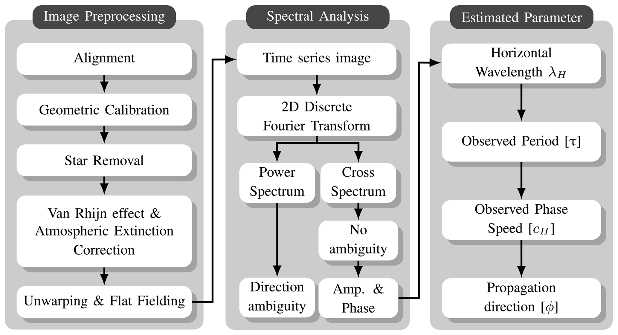
Figure 1 The flowchart shows the procedures of airglow image processing and wave parameter estimation. The three stages describe image preprocessing and processing, spectral analysis, and wave parameter estimation procedure.

For gravity wave parameters, horizontal wavelength (λ_H), phase speed (c_H), observed period (τ), and propagation direction (ϕ) are then determined using the 2D discrete fast Fourier transform (2D-DFT)-based spectral analysis (Garcia et al., 1997; Wrasse et al., 2007). Before the application of the 2D-DFT, regions of interest (ROI) with visible waves (clear dark and bright bands) were then selected. Afterward, a time series of 10 images was constructed with the selected ROI, and the 2D-DFT was applied to the ROI in the selected image time series. From the cross-spectrum of the 2D-DFT, the amplitude and phase of the wave are estimated and used to calculate the λ_H, c_H, τ, and ϕ. The power spectrum can also be used to estimate the amplitude and phase. However, the propagation direction is ambiguous, so for this work, the cross-spectrum is used. In Fig. 2, the outcome of the final image after the image preprocessing is shown. Details on the spectral analysis can be found in Wrasse et al. (2007), Bageston et al. (2011), Giongo et al. (2020), and Nyassor et al. (2021).

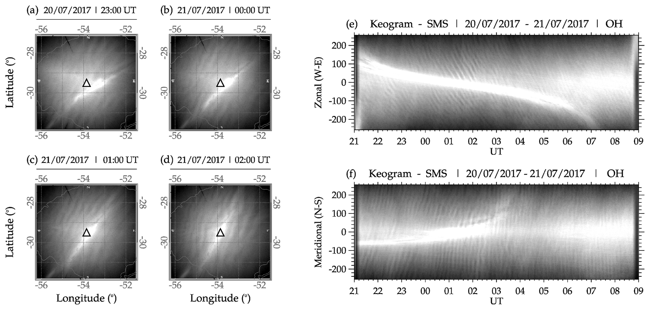
Figure 2 The observed quasi-monochromatic gravity wave (QMGW) on 20 to 21 July 2017 at São Martinho da Serra.

In Fig. 2, a sample of four preprocess images at 23:00:01, 00:00:49, 01:00:16, and 02:01:04 UT plotted on the geographic map is presented in panels (a), (b), (c), and (d), respectively. The white triangle with a black outline shows the center of the all-sky image and the location of the imager. The gray lines in panels (a), (b), (c), and (d) depict the state borders of Rio Grande do Sul. The bright strand extending from the southwest through the center of the image to the northeast is the Milky Way. In the keogram, the Milky Way is the white strand extending through the middle throughout the observation. It is important to mention that the keograms presented here are only used to show the presence of the QMGWs throughout the observation time from 21:00 UT on 20 July 2017 to 09:00 UT on 21 July 2017. It can be seen that the wave packet changes in direction with time from the northwest to the southwest. An animation of the propagation of the 20–21 July 2017 QMGW event between 21:00 UT on 20 July 2017 and 09:00 UT on 21 July 2017 is provided in the Video supplement (see the end of the paper). In Fig. 2e and f, the zonal and meridional components of the keogram, with a downward-phase progression of black and white undulations, can be seen in the zonal component. The vertical black and vertical white undulations have an upward-phase progression in the meridional component of the keogram. This clearly shows the presence of a quasi-monochromatic structure throughout the night.

3.1 Ray-tracing model

A ray-tracing model was used to investigate the propagation conditions of QMGWs and their source locations. In this work, the ray-tracing model follows the approach of Vadas (2007), Paulino et al. (2012), and Nyassor et al. (2021), with the underlying formalism from Lighthill (1978). However, in this version of the ray-tracing model, kinematic viscosity and thermal diffusivity (Vadas, 2007) are incorporated in the group velocities, and the dispersion relations are similar to the work of Vadas and Fritts (2005). The longitude, latitude, and altitude (at 87 km) of the first visible crest/trough and the observation time of the wave are assumed as the initial positions and times of the wave, and the wave characteristics are then used as the input parameters for the model.

The next step, thus, in longitude, latitude, altitude, and time of the iteration, which formed six ordinary differential equations, was solved using the fourth-order Runge–Kutta method (Press et al., 2007). An initial altitude step size of 0.2 km was set, and the subsequent step sizes were determined from $z=c_{{\mathrm{g}}_z}t$, with the boundary conditions of Paulino et al. (2012) imposed. The next step of iteration is conducted if the following criteria are satisfied:

• 1.

  The group velocity of the GWs must be less than or equal to 0.9 times the speed of sound (c_g≤0.9Cs).

• 2.

  To evaluate the effect of the background wind on the wave propagation, the real component of the intrinsic frequency must be greater than zero (ω_Ir>0).

• 3.

  The momentum flux along the wave trajectory is evaluated in relation to molecular viscosity and thermal diffusivity, since they become important dissipative processes with increasing altitude. GWs tend to dissipate when they attain maximum momentum flux; therefore, for a propagating GW, $R_{\mathrm{m}}>{\mathrm{10}}^{-\mathrm{15}}{R}_{\mathrm{0}}$. Here R_m is the momentum flux at each altitude, and R₀ is the momentum flux at the reference altitude. The factor 10⁻¹⁵ was arbitrarily chosen.

• 4.

  To ensure slowly varying viscosity in time and altitude, the module of the vertical wavelength must be less than the viscosity scale $[\mid {\mathit{\lambda }}_z\mid <\mathrm{2}\mathit{\pi }/\frac{\mathrm{d}v/\mathrm{d}z}{\mathit{\nu }}]$ in that ν=μρ is kinematic viscosity, where μ is molecular viscosity, and ρ is density (Nyassor et al., 2022). The value of $\mathit{\mu }=\mathrm{3.34}\times {\mathrm{10}}^{-\mathrm{4}}{T}^{\mathrm{0.71}}$ increases with altitude, where T is temperature (Vadas, 2007).

Items (3) and (4) from in the list above are important for studying GW propagating into the thermosphere. If there is a violation of the above-defined criteria, the iteration will be interrupted, and then all the calculations end and are saved automatically. The stopping conditions are discussed in Vadas (2007) and Paulino et al. (2012).

Atmospheric background wind and temperature used in the ray tracing were obtained from the Modern-Era Retrospective and analysis for Research and Application, Version 2 (MERRA-2), data (Gelaro et al., 2017), the Horizontal Wind Model 2014 (HWM14) version (Drob et al., 2015), and the United States Naval Research Laboratory Mass Spectrometer and Incoherent Scatter Radar Exosphere (NRLMSISE-00) empirical atmospheric model (Picone et al., 2002). Due to the limited altitude range of MERRA-2 wind and temperature data, which is up to 75 km, we concatenated the MERRA-2 wind data with HWM14 at an interpolated step at each 1 km. Similarly, the temperature data of MERRA-2 and NRLMSISE-00 are also concatenated. This procedure is done to attain an altitude range from near the surface of the ground up to 100 km. Since two different datasets with different resolutions are being concatenated, there may exist discontinuities at the concatenation altitude. The discontinuities are minimized using the approach of Nyassor et al. (2022). As a result of the temporal resolution of MERRA-2, which is 3 h, an interpolation was performed for each time step of the ray-tracing iteration. The propagation of the wave through the atmosphere leading to the determination of the source location of the wave is investigated using ray tracing in a backward mode.

4 Results

4.1 Observed QMGWs

Observations of QMGWs began in April 2017 and ended in April 2022 in São Martinho da Serra. A total of 1512 nights of clear-sky images were analyzed. From 64 nights, 209 QMGW events were obtained. The monthly distribution of observed QMGWs is presented in Fig. 3. Each bar shows the accumulated QMGW cases observed each month, with the individual colors in gray showing the number of events observed each year. The color bar defines the year of observation. It can be seen from Fig. 3 that the highest number of QMGW events was observed in August, followed by July. The following section will discuss details on the distribution of the QMGW events in Fig. 3.

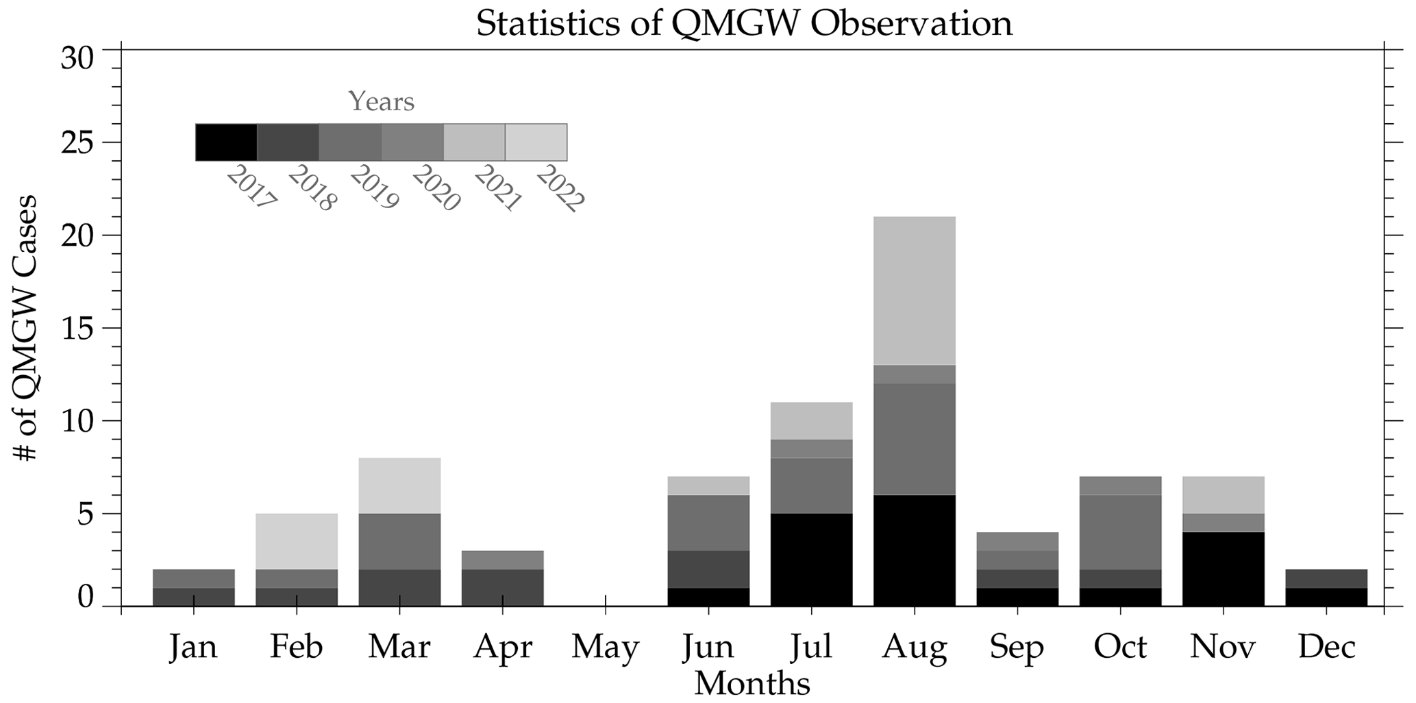
Figure 3 The observed quasi-monochromatic gravity wave (QMGW) event distribution between 2017 and 2021 at São Martinho da Serra.

4.2 Statistical distribution of QMGW events and parameters

The 5 years of observed OH airglow images were subjected to spectral analysis to estimate the QMGW characteristics. Specific criteria were imposed to select the QMGW events used in this work. After the spectral analysis, the confidence level (CL) of the estimated wave spectrum is estimated. The spectrum having peak power spectral density with CL ≥ 95 % is accepted (Hu et al., 2002). Before selecting the QMGWs, the waves must first and foremost be visible in the OH images of the entire night for not less than 2 h. Next, the wave parameters were determined every 10 min. This is done to track the variations in the wave parameters (precisely the horizontal wavelength) to ensure it is the same wave. If the criteria of CL ≥ 95 %, visibility of wave, and the determined wave being similar are satisfied, then the wave is then subjected to the following conditions:

• i.

  the λ_H must be greater than or equal to 10 km (λ_H ≥ 10 km);

• ii.

  the variation of ϕ within 1 h must be less than 25° ($\mathrm{\Delta }\mathit{\varphi }\le \pm$25°);

• iii.

  the GW propagation period must be between 5 and 80 min (5 min ≥ τ ≤ 80 min); and

• iv.

  finally, the GW phase speed must be less than or equal to 150 m s⁻¹ (c_H ≤ 150 m s⁻¹).

Note that the c_H > 150 m s⁻¹ was considered the upper limit to avoid interference with the acoustic wave spectrum. Vadas and Azeem (2021) mentioned that GWs with c_H ∼ 250 m s⁻¹ cannot propagate below 100 km. However, we chose this value, since it will take a wave with 150 m s⁻¹ approximately ∼ 12 min to travel 100 km. If all of these conditions are satisfied, then the wave is selected. On the contrary, the wave will be removed even if CL ≥ 95 % and one of the other conditions are not met. In Fig. 4, the characteristics of the selected QMGWs obtained from the spectral analysis are presented. Panel (a) shows the QMGW horizontal wavelength distribution over the 5 years of observation. Panel (b) is the distribution of the propagation period, whereas panel (c) is the histogram of the phase speed distribution. Panel (d) shows the distribution of the propagation direction of the QMGWs.

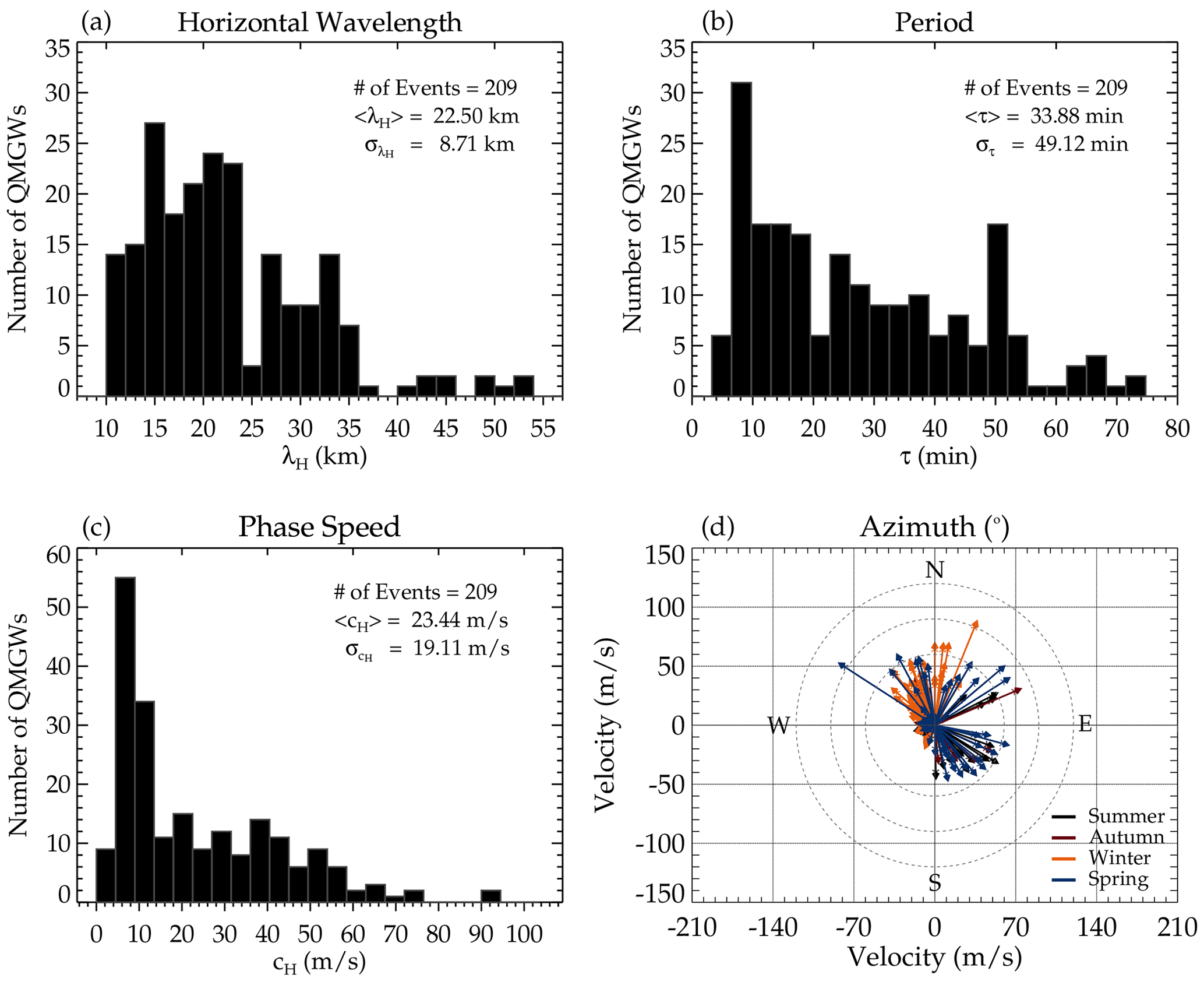
Figure 4 Quasi-monochromatic gravity wave (QMGW) characteristics over 5 years of observations at São Martinho da Serra. Panels (a), (b), and (c) present the histogram of the horizontal wavelength (λ_H), period (τ), and phase speed (c_H), respectively. In panel (d), the propagation direction (ϕ) of the QMGWs is presented according to the season.

For the λ_H distribution in Fig. 4a, an average wavelength of 22.50 km was observed with a peak value of ∼ 15 km, with a broad and dominant distribution ranging between 10 and 35 km. However, the normal distributions of the τ (Fig. 4b) and c_H (Fig. 4c) are narrow, with a dominant peak period and phase speed skewed toward ∼ 10 min and ∼ 9 m s⁻¹, respectively. The propagation direction of the QMGWs is presented in Fig. 4d. The direction of wave propagation is significantly anisotropic, mainly between northwest to northeast during the summer and in the southeasterly direction during the winter.

4.3 Ray-tracing results

Ray-tracing model is used to study the propagation of the QMGWs and to determine their possible source locations. Two wind models were considered when running the ray-tracing model: zero wind and model wind modes. The model wind mode consists of concatenated MERRA-2 and HWM14 wind. However, in this work, only the model wind result of the ray tracing is presented. The ray-tracing results for the 209 QMGW events are presented in Fig. 5. The ray paths of the QMGWs in a model wind atmosphere are shown in blue lines, and their respective stopping positions are in red squares. The open triangle shows the observation site location.

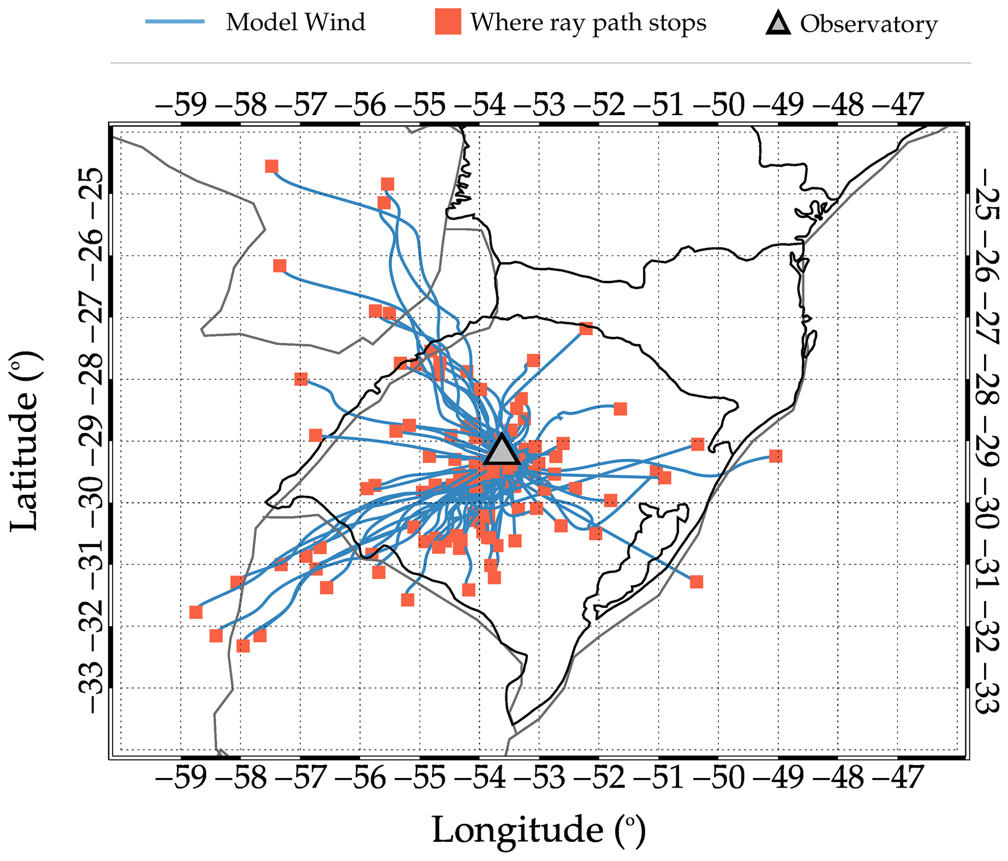
Figure 5 Backward ray paths and stopping positions of the observed quasi-monochromatic gravity waves (QMGWs) over São Martinho da Serra.

The propagation time of the waves from their source to the observation altitude in the mesosphere is presented in Fig. 6a, while the duration of propagation (thus the time span of visibility of the propagating waves in the OH images during the night) of the waves in the OH images is presented in Fig. 6b. It can be seen that majority of the waves propagated less than 1 h from the source position in the lower atmosphere to the OH emission layer. Similarly, the observed wave packet from which the individual QMGWs were selected in the OH airglow images were visible over the field of view of the all-sky imager and propagated for 2–3 h.

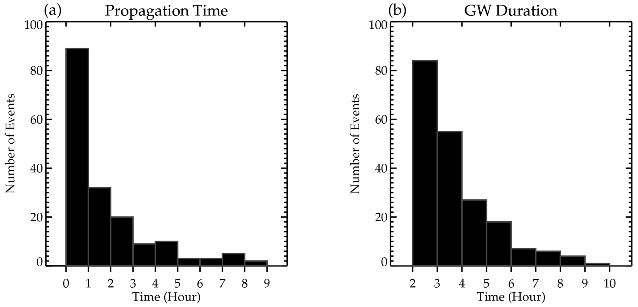
Figure 6 Propagation and visibility times of the quasi-monochromatic gravity waves (QMGWs). (a) The propagation time of the wave from the source position to the OH emission layer. (b) The duration of propagation of visible QMGWs in the OH images.

4.4 Wave sources

Most mesospheric GWs have their primary sources in the lower atmosphere. Various generation mechanisms, such as the mechanical oscillator effect, obstacle effect, and latent heat of deep convection and orographic, are known to be prominent source mechanisms (Fritts and Alexander, 2003). From the ray-tracing result presented in Fig. 6, it was observed that 12.4 % of the ray path stopped above 60 km. This implies that these waves were generated in situ but not in the troposphere. However, the source mechanisms of these waves will not be discussed in this current work. On the other hand, the ray path of the remaining 87.6 % stopped in the troposphere. It indicates that this percentage of the wave is most probably generated in the troposphere. Figure 7 presents the distribution of the minimum cloud-top brightness temperature near the stopping positions of the ray paths in the troposphere.

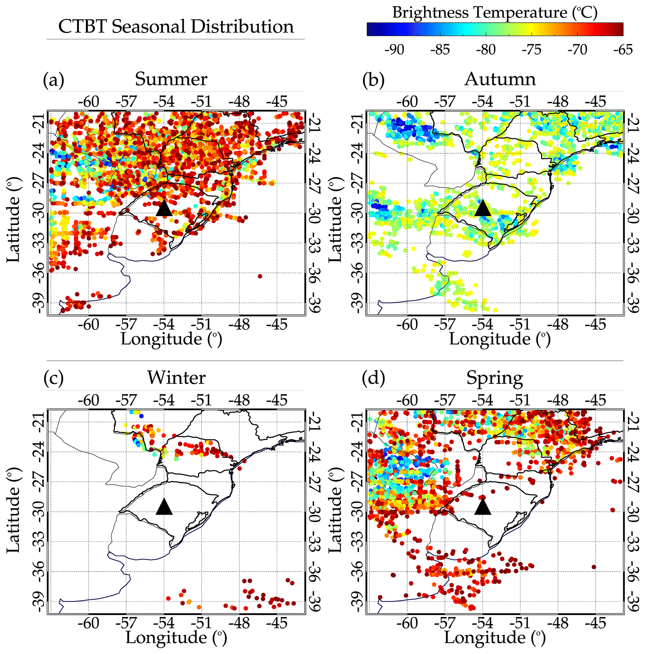
Figure 7 Seasonal distribution of the cloud-top brightness temperature (CTBT) close to the stopping locations of the ray paths in the tropopause.

Panels (a), (b), (c), and (d) show the seasonal distributions of CTBT for summer, autumn, winter, and spring, respectively. The selection time of the CTBT ranges from 18:00 to 06:00 UT on the following day. The selection of this time range was due to the observation time of the QMGWs and possible excitation time determined by the ray tracing. The overall distribution of the CTBT for each season agrees with the propagation directions presented in Fig. 4d.

5 Case studies

5.1 Case study of 20–21 July 2017 event (case study 1)

On 20 July 2017, at around 22:00 UT, GW structures with λ_H ∼ 10–60 km were observed in the OH airglow propagation towards the northwestern direction. The waves with similar wavelengths gradually propagated toward the west and southwest as time progressed. In Fig. 8, the sub-panels labeled (i) show the λ_H at each 1 h, whereas the sub-panels labeled (ii) show the variation in ϕ at each hour. The sub-panels labeled (iii) show the variation of ϕ in a polar plot representation. Panels (a), (b), and (c) with the sub-panels labeled (i) depict the variation of λ_H between 30–40, 40–50, and 50–60 km of the GWs with time. The corresponding sub-panels labeled (ii) and (iii) of each panel represent the azimuth versus time and azimuth in a polar plot. The color representing λ_H in the sub-panels labeled (i) at each hour corresponds to the same color in the sub-panels labeled (ii) and the arrow in the sub-panels labeled (iii).

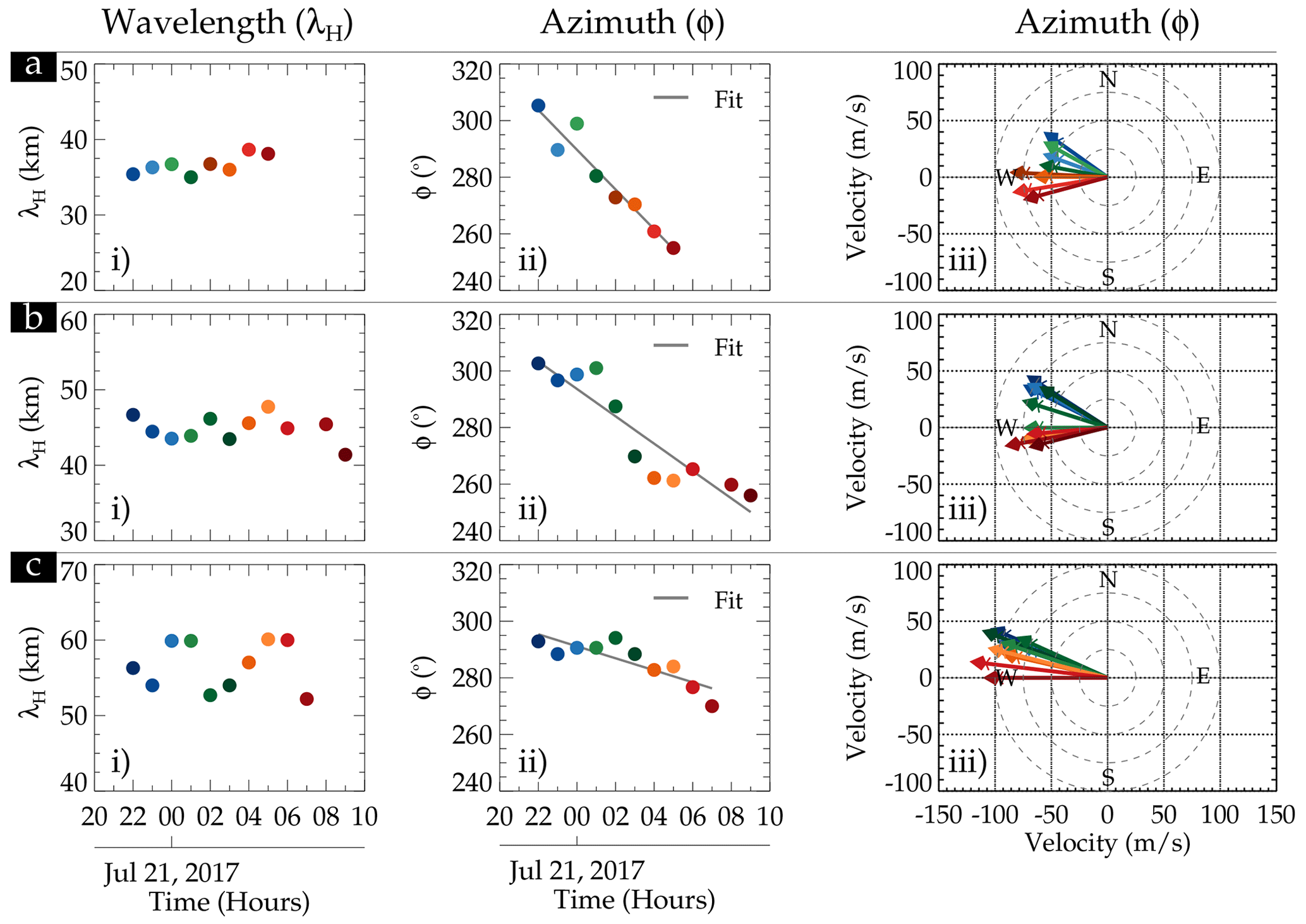
Figure 8 Variations in horizontal wavelength of 30–60 km gravity waves and the propagation directions. The sub-panels labeled (i), (ii), and (iii) are the λ_H, azimuth, and azimuth versus phase velocity in a polar plot.

We observed that the maximum variations in the three groupings of the wavelengths are within ±5 km. These variations fall within the average error range of each group. In relation to the variation in the azimuth with time, the change in the propagation direction is evident that all the groups of the wave propagated from the northwest at the beginning of the observation to the southwest at the end. The variations in the propagation direction in the sub-panels labeled (ii) were affirmed in the polar plots in the sub-panels labeled (iii).

5.1.1 Ray-tracing result

Figure 9 shows the ray-tracing results of the 29 QMGWs in the event observed on 20–21 July 2017. The color bar represents the number of each of the 29 waves. The hourly mean λ_H of the three λ_H groupings were ray traced from the OH emission altitude. In Fig. 9a, the horizontal dashed line indicates 87 km, whereas the dot with similar colors to the model wind ray path of the wave is the reflection point. The squares in Fig. 9b represent the position where the wave stops.

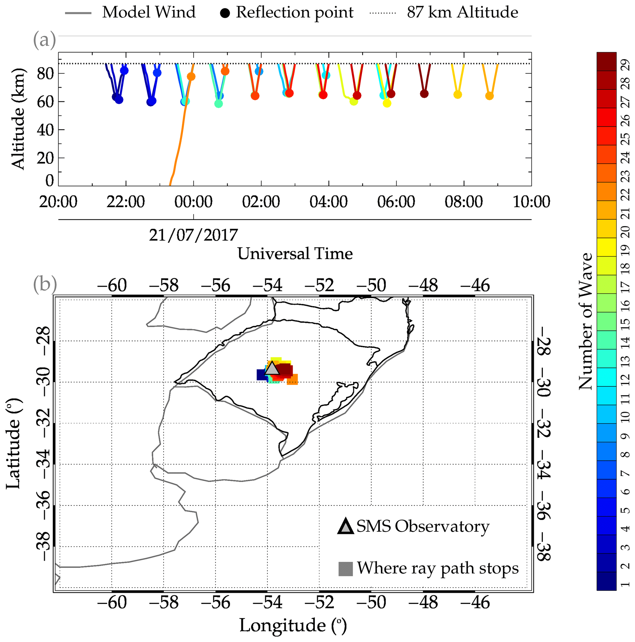
Figure 9 Ray-tracing results of the quasi-monochromatic gravity waves on 20–21 July 2017.

Figure 9a shows that the ray tracing started at 87 km. However, we observed that almost all the waves reflected. According to Vadas (2007), a reflection of GWs occurs where and when the Brunt–Väisälä frequency (N) is nearly equal to the intrinsic frequency (ω_I) of the wave. This result showed that, except for wave no. 21 (see Fig. 9a), which reached the troposphere, the others reflected between 60 and 85 km. The reflection of these waves suggests the possibility of an evanescence layer (m<0). The subject of the ducting will be discussed in the following section in order to verify if there exists an evanescent layer. In panel (b), the position of the reflection in space is distributed around the observation site, showing that the GWs did not travel far horizontally. Even wave no. 21 propagated to the troposphere only 100 km from the observation site. The stopping point of this wave is not close to any convective system at the time when the ray path reaches the tropopause.

5.1.2 Convective sources

Figure 10 shows the minimum cloud-top brightness temperature (CTBT) distribution in space between 18:00 UT on 20 July 2017 to 06:00 UT on 21 July 2017 and the vertical distribution of CTBT with an overshooting top (OT) height.

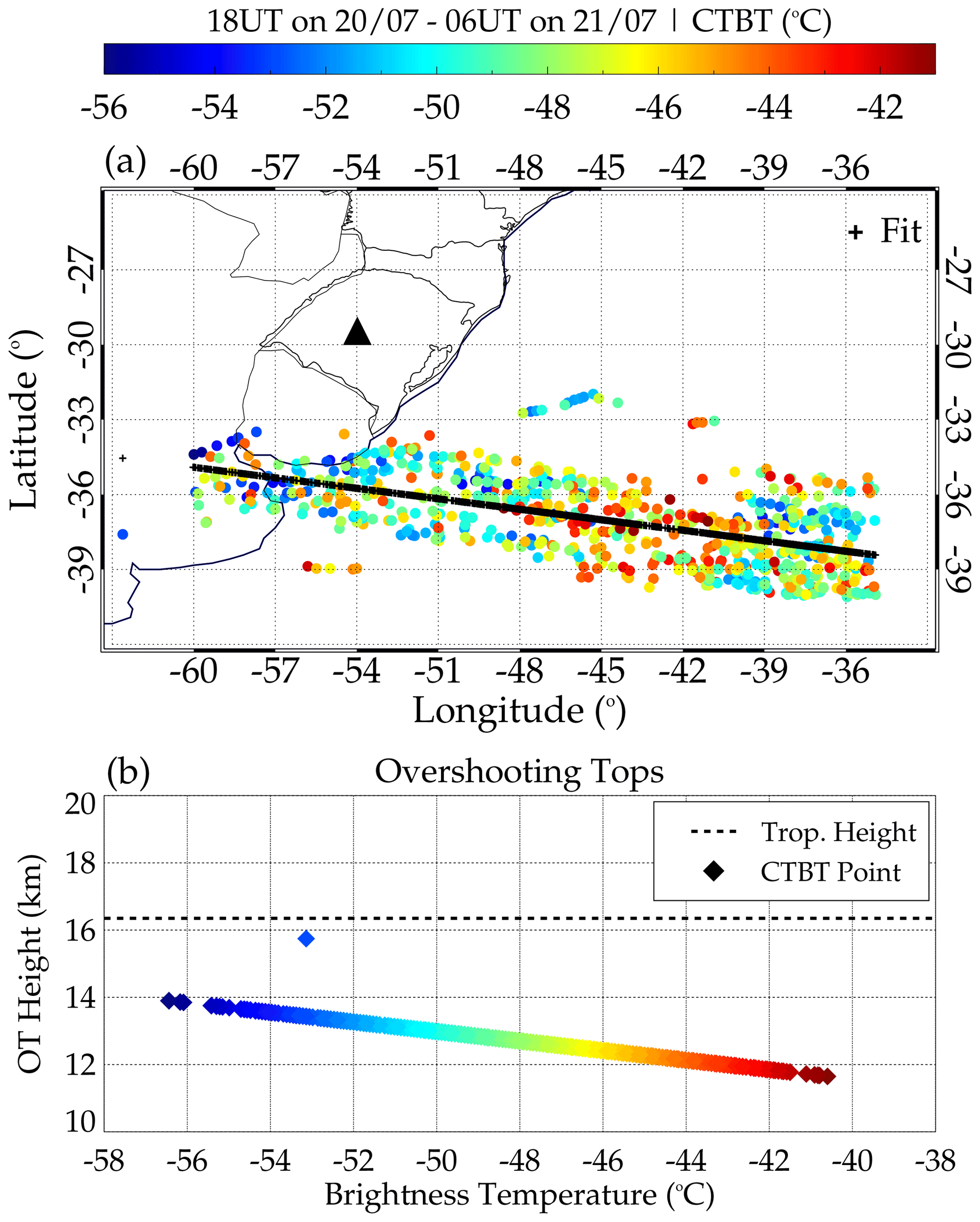
Figure 10 Distribution of (a) minimum cloud-top brightness temperature (CTBT) in space and time between 18:00 on 20 July 2017 to 06:00 on 21 July 2017 and (b) CTBT with OT height.

The minimum CTBT within longitude −63 to −33° and latitude −42 to −24° is determined for each 1° × 1° grid box from 18:00 UT on 20 July 2017 to 06:00 UT 21 July 2017, as shown in Fig. 10a. The composite plot of all the CTBTs is then plotted over the map to see their distribution relative to the stopping positions of the ray path. We observed, in Fig. 10, that the closest CTBT to the ray path stopping position is ∼ 300 km for wave no. 21, which reached the troposphere. It is important to state that the other waves reached a minimum of 60 km altitude. Therefore, Fig. 10a shows that these waves unlikely originated from the convective system. It is because no CTBT in Fig. 10a overshot, as shown in Fig. 10b.

The tropopause height obtained from a radiosonde sounding at Santa Maria (29.69° S, 53.27° W) on 21 July at 00:00 UT was ∼ 16.35 km. The highest overshooting top within the time range considered was ∼ 16 km. Several research works (e.g., Nyassor et al., 2021, and references therein) showed that GWs can be generated through the overshooting of the tropopause (mechanical oscillator mechanism). However, for this mechanism to be feasible, the CTBT must be colder than the tropopause temperature signifying overshooting of the tropopause. This result therefore implies that overshooting of the tropopause is not the source mechanism of the waves observed on 20–21 July 2017. Fritts and Alexander (2003) mentioned that a convective system could also generate GWs through three mechanisms, namely latent heat, obstacle effect, and mechanical oscillator effect. Knowing that the mechanical oscillator effect is not responsible for generating the GWs on 20–21 July 2017, the other mechanism will be explored later in the paper.

5.2 Case studies of 15–16 August 2017 (case study 2) and 20–21 August 2017 (case study 3) events

Similar to the 20–21 July 2017 event, GW structures with λ_H ∼ 30–50 km were observed in the OH airglow images propagating toward the northwesterly direction. Contrarily, these waves propagated mainly toward the northwest throughout the entire night. The variation in the λ_H and ϕ values at each 1 h and the ϕ in a polar plot are presented in Fig. 11. The sub-panels labeled (i), (ii), and (iii) have the same meaning as defined in Fig. 8. Panels (a) and (b) depict the sub-panels labeled (i), (ii), and (iii) for λ_H between 30–40 and 40–50 km for the 15–16 August event, respectively, whereas panels (c) and (d) show that of the 20–21 August event.

In the sub-panel labeled (i) in panel (a), no significant variations were observed in the λ_H. The propagation direction (ϕ) showed some variation with time but generally (the fit is the solid black line) varies from north to northwest. Even though the 40–50 km GWs lasted for just 3 h, it is clear that this GW was propagating mainly in the northwestern direction (see the sub-panels labeled ii and iii for panel b). The characteristics of these GWs clearly show that their source may be the same.

The GW structures observed on 20–21 August 2017 have a similar range of λ_H to that of 15–16 August 2017. The two wavelength group (30–40 and 40–50 km) variations in the λ_H and the respective ϕ (in time and polar plot) are presented in panels (c) and (d) of Fig. 11. Like the propagation direction of the waves in Fig. 10a and b, the wave (30–40 km) in Fig. 11c propagates in a similar direction. However, the 40–50 km wave propagated from the northwesterly to the northerly direction. The different propagation directions of the wave in this spectrum suggest that this wave might be excited by a different source. The propagation of these GWs is studied, and their possible source location is investigated using the ray-tracing result presented in Fig. 12.

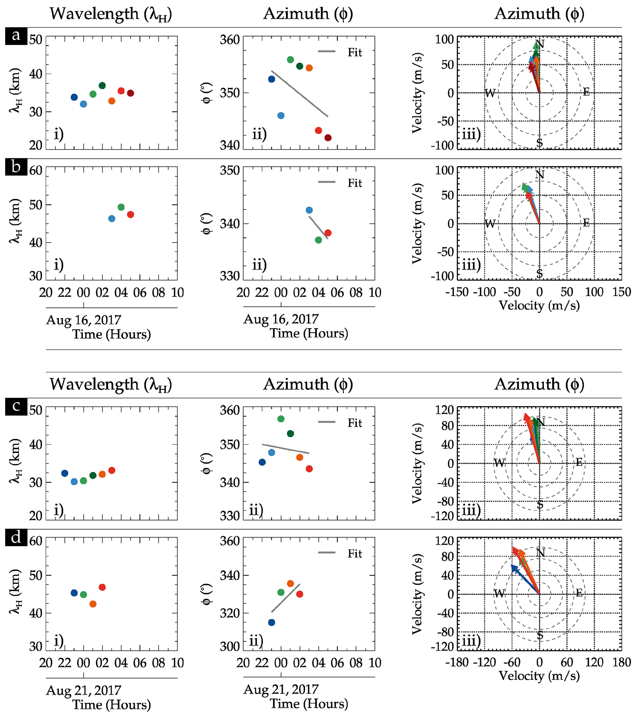
Figure 11 Similar to Fig. 8 for only 30–50 km wavelength gravity waves. The sub-panels labeled (i), (ii), and (iii) are the λ_H, azimuth, and azimuth in a polar plot. The case study of 15–16 August 2017, is presented in panels (a) and (b), whereas that of 20–21 August 2017 is presented in panels (c) and (d).

5.2.1 Ray-tracing results of 15–16 and 20–21 August 2017 GW events

Figure 12 presents the ray-tracing result of the 15–16 and 20–21 August 2017 QMGW events. In total, 10 GWs were ray traced for each wave of the event. For the 15–16 August event, Fig. 12a showed that wave nos. 6, 7, 8, 9, and 10 propagated to the troposphere. Wave nos. 1, 2, 4, and 5 reflected at around 10 km, whereas wave no. 3 reflected at 60 km. For the ray path of the wave in space (see Fig. 12b), all the ray paths stopped at the southwestern part of the SMS observatory. This is an indication that the waves are most likely excited in the southwestern part of Rio Grande do Sul or the northeastern part of Uruguay.

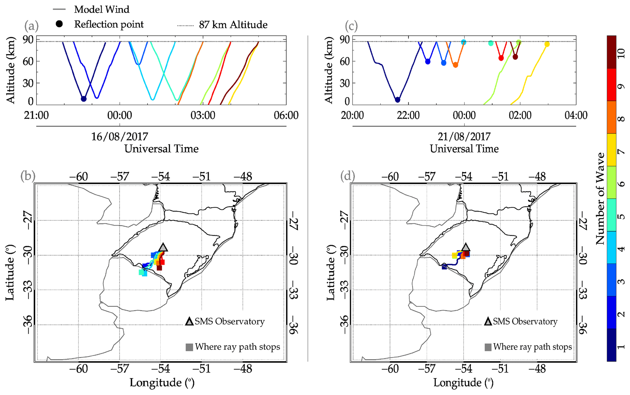
Figure 12 Ray-tracing results of the quasi-monochromatic gravity waves on 15–16 and 20–21 August 2017 events.

In Fig. 12c, we observed that all 10 waves reflected at a point. Wave nos. 4, 5, 6, and 7 reflected first at the OH emission altitude, among which wave nos. 6 and 7 propagated to the troposphere. Wave nos. 4 and 5 could not propagate further upwards or downwards. Wave nos. 2, 3, 8, 9, and 10 also reflected between 60 and 70 km. Wave no. 1, however, reflected ∼ 5 km. As presented in Fig. 12d, the propagation of these waves in space showed that the waves are also generated in the southwestern part of the observation.

5.2.2 Convective sources

Figure 13 shows the CTBT maps and the OT heights from 18:00 UT on 15 August to 06:00 UT on 16 August (panels a and b) and 18:00 UT on 20 August to 06:00 UT on 21 August (panels c and d) for case studies 2 and 3. The CTBT distribution in Fig. 13a corresponds to the ray-tracing result in Fig. 12b, whereas Fig. 13d corresponds to that of Fig. 12d. From this plot (i.e., Fig. 13), it has been observed that the distribution of the CTBT around the southwestern part of the observatory and the northeastern part of Uruguay agrees with the stopping positions of the ray-traced path. In particular, the ray-tracing results in Figs. 12b and 13a showed a clear correlation. Even though most of the ray paths in Fig. 12c are reflected in the lower mesosphere, the ray paths that reached the troposphere agree with the CTBT distribution. In both cases, the CTBT maps showed no strong convective activity. This is seen in the brightness temperature of the individual CTBT scales shown in the color bar.

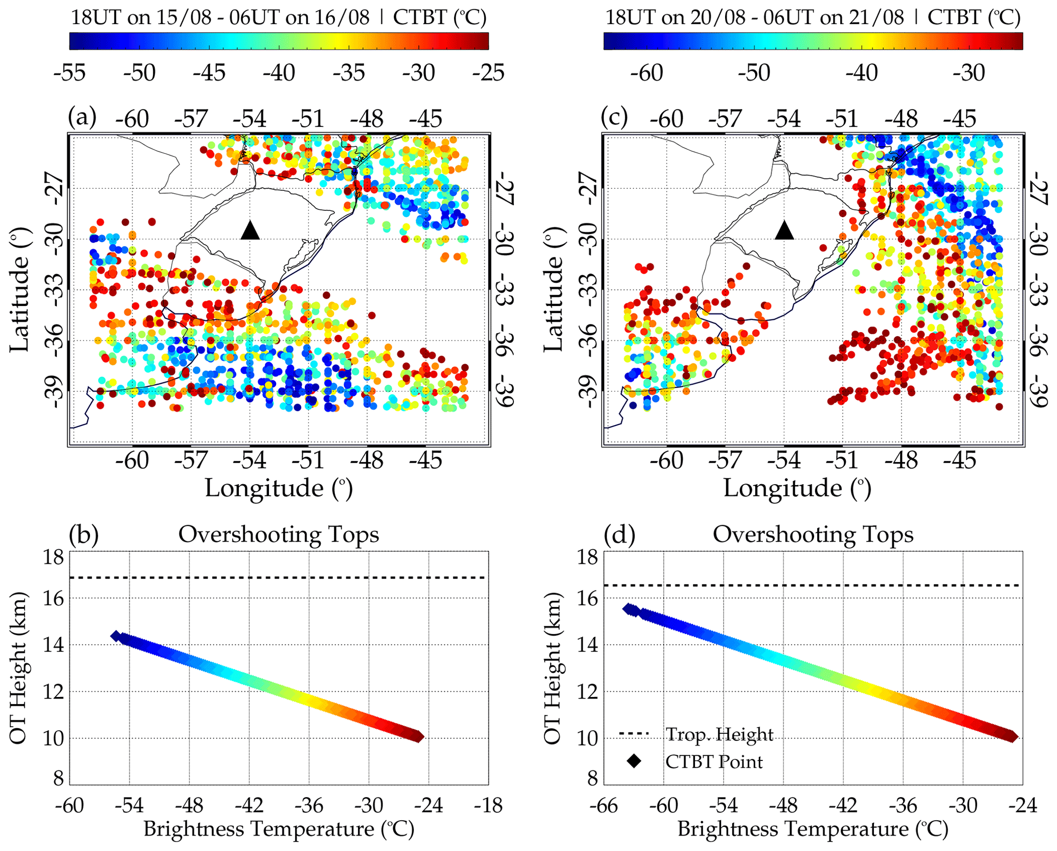
Figure 13 Distribution of (a) minimum cloud-top brightness temperature (CTBT) in space between 18:00 on 15 August 2017 and 06:00 on 16 August 2017 and (b) CTBT with OT height. (c) CTBT in space between 18:00 on 20 August 2017 and 06:00 on 21 August 2017 and (d) CTBT with OT height.

In Fig. 13b and d, the individual OT heights are plotted as a function of brightness temperature. It can be observed that throughout the 12 h, no CTBT/OT values were higher than the tropopause height. This indicates that no overshooting by the convective system occurred; hence, the mechanical oscillator effect of GW excitation cannot be the mechanism that excited these waves. However, other mechanisms can be the GW excitation mechanism of these waves. The general characteristics of the convective system during these nights showed characteristics of the activities of cold fronts. Next, other mechanisms that can excite the observed waves are investigated.

5.3 Lightning distribution

Lightning activity is used to indicate the severity of deep convection. Nyassor et al. (2021, 2022) used lightning distribution in space to show the direct relationship to CTBT. Nyassor et al. (2021, and references therein) used the lightning rate as an indicator of overshooting of the tropopause, while investigating the sources of three concentric gravity events. Strong correlations were observed between the lightning rate and overshooting tops in space and time. In this study, the lightning activity in space (Fig. 14) and time (not shown) were used to show whether the convective system present during the three case studies was active.

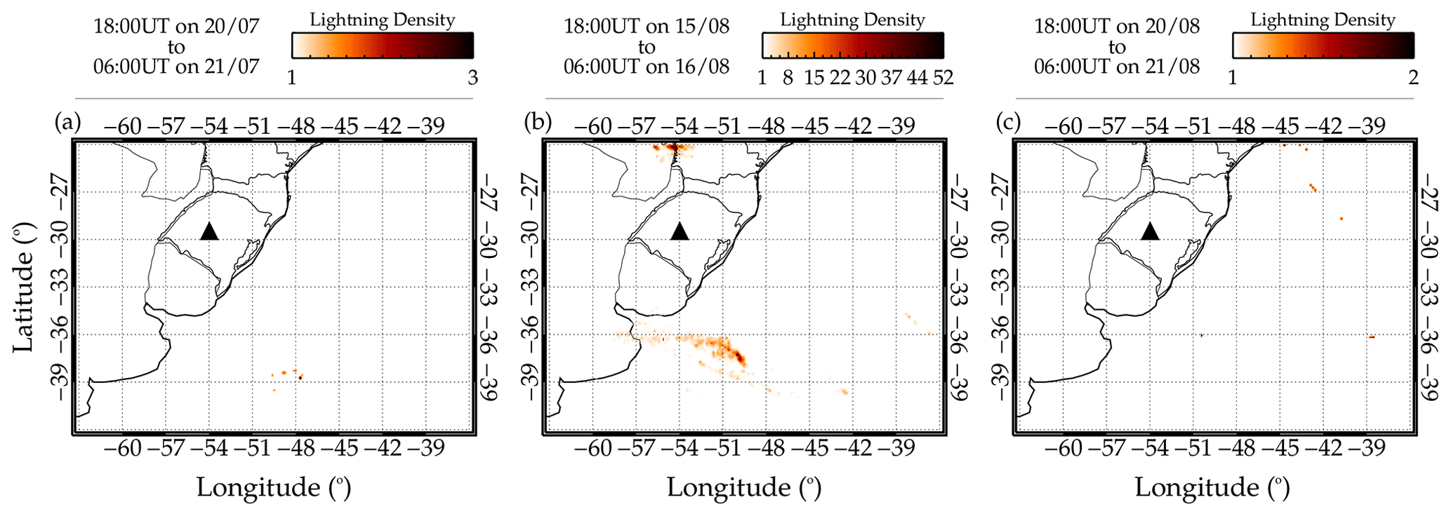
Figure 14 Lightning activities during the quasi-monochromatic gravity wave (QMGW) case studies 1, 2, and 3. The lightning activity distribution during case study 1 is shown in panel (a) and case study 2 in panel (b), and in panel (c) is that of case study 3.

To determine the lightning density, we binned the lightning flashes by 0.15° × 0.15° in longitude and latitude (Nyassor et al., 2021, 2022) from 18:00 to 06:00 UT. The density distribution was then overplotted on the map, as shown in Fig. 14. Interestingly, the density distribution of the lightning during these case studies is low, especially for the cases of 20–21 July and 20–21 August. The maximum density distribution occurred during the 15–16 August event (Fig. 14b). However, the distribution of this event is far from the ray-traced source locations. In general, the density distributions of the three events are low. This is another indication that these convective systems were not active. Even though the lightning distribution of the 15–16 August QMGW event (Fig. 14b) was relatively high, the lightning rate (not shown) did not present characteristics of overshooting. Using lightning activity, it has been further proven that the observed waves are not excited through the overshooting mechanism.

6 Background conditions on the propagation of the case studies

The propagation of GWs is controlled by the atmospheric background field, especially wind, and temperature. The state of the wind and temperature determine whether a wave is propagating or evanescence (ducted or trapped) (Gossard and Hooke, 1975). Ducted GWs can propagate horizontally for long distances without losing energy (Bageston et al., 2009). Bageston et al. (2009) and Fechine et al. (2009) showed that ducted waves due to either Doppler or thermal duct enhance the longer horizontal propagation of GWs over a long duration. Thermal ducts are formed when there is a temperature inversion layer, whereas the Doppler duct is formed when a wind shear exists. A dual duct is formed when both the temperature inversion layer and wind shear exist at the same altitude (e.g., Chimonas and Hines, 1986; Isler et al., 1997; Nappo, 2013; Walterscheid et al., 1999).

During these three case studies, temperature profiles obtained from SABER (Sounding of the Atmosphere using Broadband Emission Radiometry) showed an inversion layer within 60 to 90 km. The case studies of 20–21 July, 15–16 August, and 20–21 August have a mesospheric inversion. Also, vertical shear was present in the zonal wind. Therefore, the ducting condition was determined by utilizing the SABER temperature profile and the concatenated wind profiles obtained from MERRA-2 and HWM14.

In Fig. 15, the background analysis of the propagation characteristics of the 20–21 July 2017 QMGW event is presented. The SABER temperature profile and its corresponding potential temperature are presented in panel (a). The Brunt–Väisälä frequency profile was estimated using (Fritts and Alexander, 2003),

$$\begin{array}{}\text{(2)}& N=\sqrt{-{\displaystyle \frac{g}{\mathit{\theta }}}{\displaystyle \frac{\mathrm{d}\mathit{\theta }}{\mathrm{d}z}}},\end{array}$$

which is presented in panel (b), with θ being potential temperature, g the gravitational acceleration, and z the altitude. In panel (c), the wind in the direction of the wave for propagation directions of 315, 290, and 270° is shown, whereas the profile of the vertical wavenumber squared (m²), adapted from Vadas and Fritts (2005), is shown in panel (d).

Figure 15 Propagation characteristics during the 20–21 July 2017 QMGW case study.

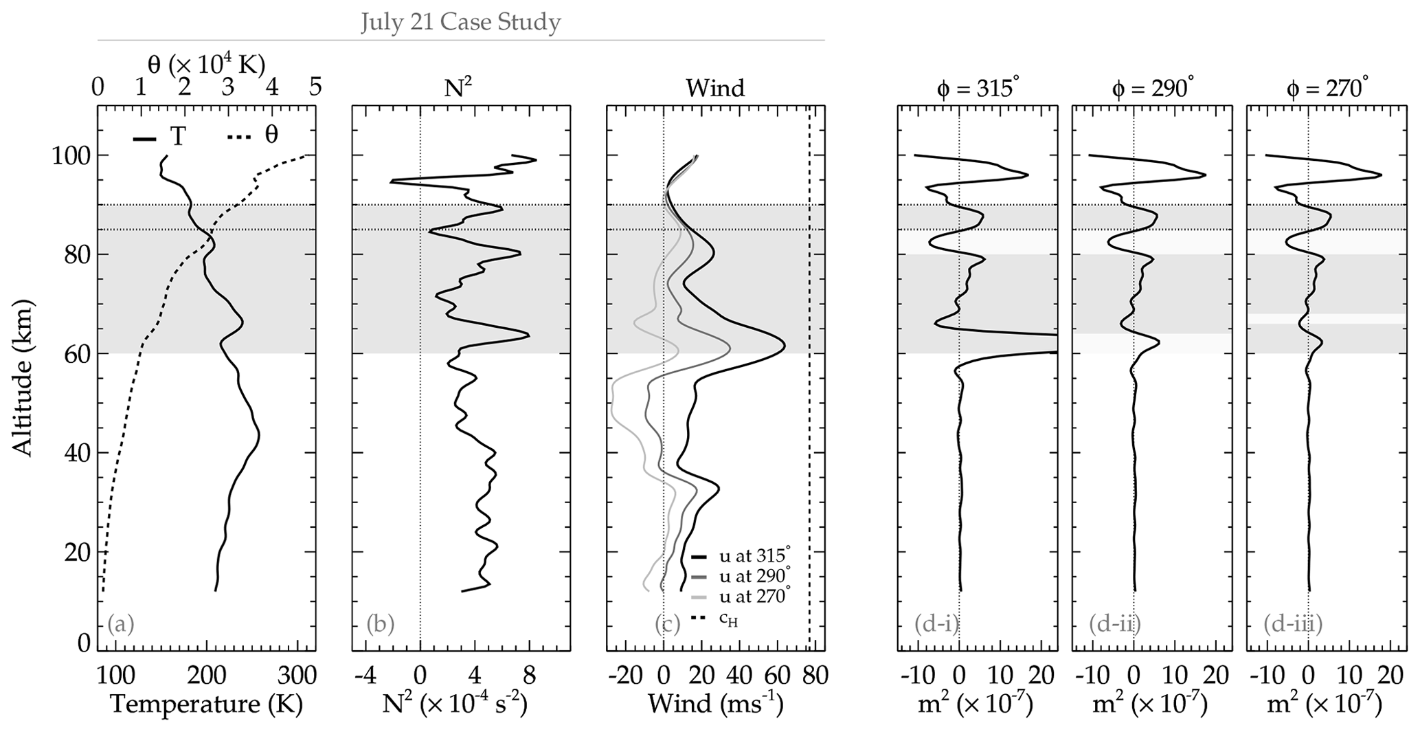
Panel (d) has three sub-panels labeled (i), (ii), and (iii). These sub-panels represent the directions of propagation of the wave. As seen earlier in Fig. 8, the wave in this case study propagated from northwest to southwest. As a result, propagation directions in 315, 290, and 270° are considered to verify if a duct exists in all directions during the propagation of the wave.

From the analysis in Fig. 15, it is seen that a duct exists in all three propagation directions considered. The existence of the duct implies that the background atmosphere creates the necessary condition favorable for the wave to propagate in this region for a long distance and time. During this QMGW event, the propagation of the observed wave for about 9 h with almost the same horizontal wavelength suggests that there is (a) a possible propagation in a duct and that there is (b) a source emitting GWs at a constant spatial and temporal scale over a long time. Regarding the longer horizontal propagation, the presence of the duct affirms the longer propagation of these QMGWs with similar spatial characteristics from the beginning to the end of the observation. Various researchers have used ducts (e.g., Xu et al., 2015) to explain the longer horizontal propagation of the wave reported in their work. Similar to the result of Xu et al. (2015), and references therein, it can be concluded that the 20–21 July 2017 event was ducted, hence causing the longer propagation over such a long time.

A similar analysis is conducted for the 15–16 and 20–21 August QMGW cases, as shown in Fig. 16. The profiles of the parameters in panels (a) and (b) are similar to that of Fig. 15, except for panels (c) and (d), where the vertical wavenumber squared (m²) of only a single propagation direction obtained in panel (c) is presented. In both case studies, the m² (vertical wavenumber squared) profile showed two ducts between altitude ranges of 75–95 km. The ducts of these two cases are not precisely within the peak of OH emission layer altitude (i.e., 87 km) and are narrower than that of 20–21 July 2017. However, these ducts can support a longer horizontal propagation of the observed QMGWs.

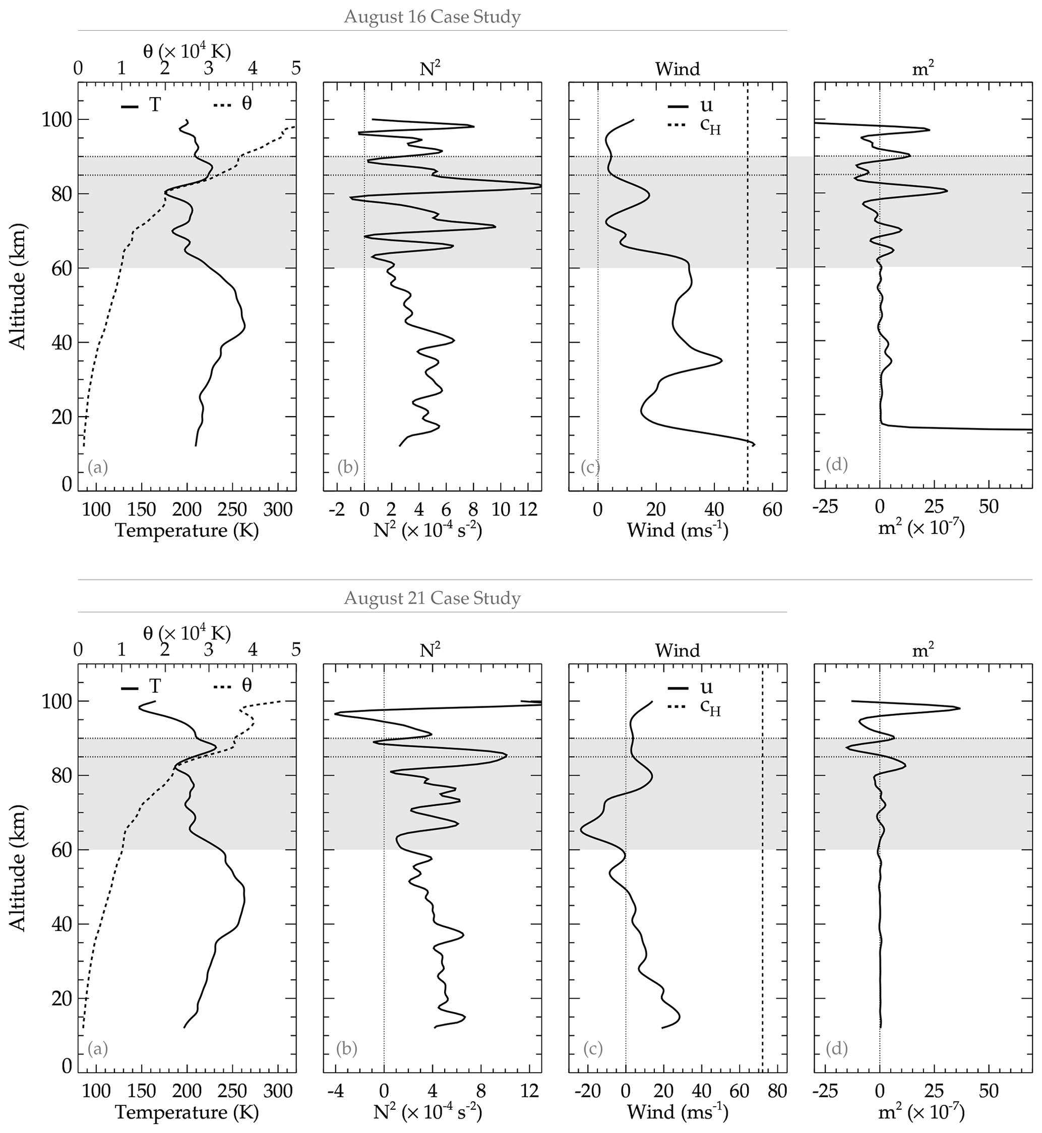
Figure 16 Propagation characteristics during the 15–16 and 20–21 August 2017 QMGWs case studies.

In Fig. 12, the ray-tracing result of the 15–16 August case studies (panels a and b), except for one of the waves (i.e., wave no. 3) of the remaining nine, reached the troposphere. This indicates that these waves were excited in the lower atmosphere and in the southwest of the observation site, with wave nos. 6, 7, 8, 9, and 10 first reflecting around 60 km. Similarly, in panels (c) and (d), the ray-tracing result showed that only three waves reached the troposphere. The remaining waves reflected above the altitude of 60 km. These propagation characteristics, however, indicate that the condition, that is, $c_{\mathrm{H}}=N/k+U$, for reflection, is satisfied here (Heale and Snively, 2015).

The ray-tracing results for the three case studies could not capture the trapping of the waves but could only capture the reflection because the phase front of the wave and the background wind are the same. Also, the zonal component of the wind during these events peaked within 60 to 70 km. In a simulation study conducted by Heale and Snively (2015) for small-scale gravity waves (SSGWs), they found that their simulated wave ray path reflected along the largest-magnitude negative phase front of the background wind. All this evidence showed that most of the observed QMGWs are ducted, thus allowing longer propagation. Next, we investigate the source and related mechanisms that emitted the spectrum of waves observed in the mesosphere.

7 Other wave sources and source mechanisms

7.1 Cold fronts

A cold front is the leading edge of a cooler air mass at ground level that replaces a warmer air mass and lies within a pronounced surface trough of low pressure. A cold front generates a cumulous cloud with precipitation, emitting GWs. Since the systems for case studies 1, 2, and 3 are not overshooting, further analysis of the characteristics of the system is conducted using GOES images to study the cold-front characteristics. According to Schmit et al. (2017), among the GOES-16 products, channel 10 captures the activities of the lower/midlevel water vapor (fronts) between 500 and 750 hPa (2.5–5.5 km) in the infrared wavelength at 7.3 µm.

Figure 17 presents a 3 h resolution time series of GOES-16 infrared images of a cold front between 18:00 UT and 06:00 UT. Figure 17a–d presents the spatiotemporal evolution of the cold front during the 20–21 July 2017 case study, whereas panels (e)–(h) and (i)–(l) of Fig. 17 present that of the 15–16 and 20–21 August case studies, respectively. The time of each image is written in the upper-left corner. The color bar in the upper left shows the temperature scale of the cold front. Cold fronts are used, among others, to monitor severe weather potential. For this reason, complementary data such as reanalysis and spaceborne observation were used to investigate the possibility of severe weather.

First, convective available potential energy (CAPE), an essential parameter in predicting severe weather, is used. From CAPE, the maximum updraft velocity ($w=\sqrt{\mathrm{2}\cdot \mathrm{CAPE}}$) is mainly used to determine possible overshooting of the tropopause that can lead to gravity wave excitation. As discussed earlier, no overshooting was observed before the observation of these case studies. However, to confirm that no overshooting was observed, CAPE maps within the same time and spatial range, as shown in Fig. 17, were plotted and presented in Fig. 18. The color bar in the upper-left corner shows the values of CAPE.

In Figs. 17 and 18, the contour lines of omega ($\mathrm{d}p/\mathrm{d}z$) at 850 hPa were overplotted on the cold front and CAPE maps. In Fig. 17, the contour lines and their magnitude are represented in red, whereas in Fig. 18, they are in gray lines. The omega data were obtained from the National Centers for Environmental Prediction (NCEP). More details on the omega data can be seen elsewhere in Kanamitsu et al. (2002). The following section will discuss the omega contours, the cold front, and CAPE. The omega is plotted over the cold front and CAPE maps to show the regions with cold brightness temperature and high CAPE values to show strong upward vertical air motion. The omega (upward vertical motion of air mass) in gray contour lines is overplotted on the spatiotemporal evolution of the CAPE maps. Even though, in Figs. 17 and 18, omega at 850 hPa was overplotted on the cold front and CAPE maps, the following question still remains: what are the characteristics of omega with altitude?

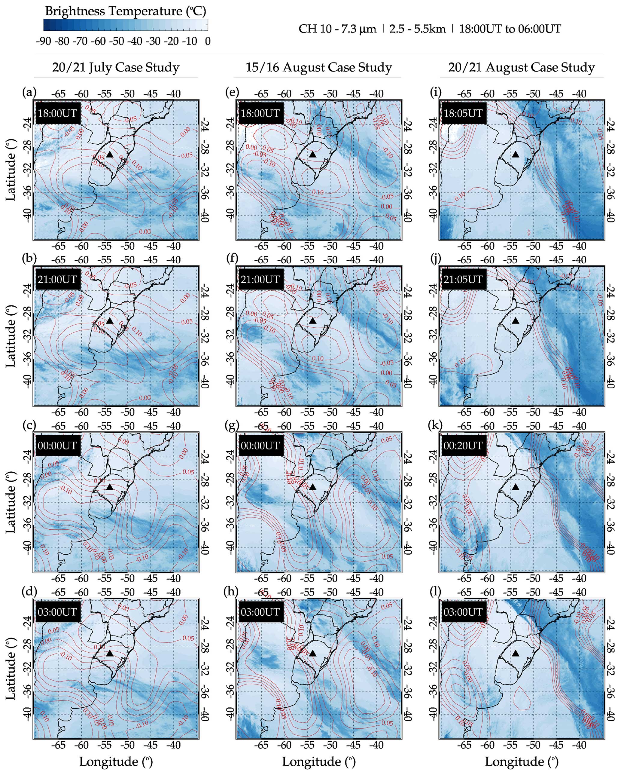
Figure 17 Spatiotemporal evolution of cold front in GOES-16 channel 10, 7.3 µm, with the omega (upward vertical motion of air mass) overplotted in red contour lines.

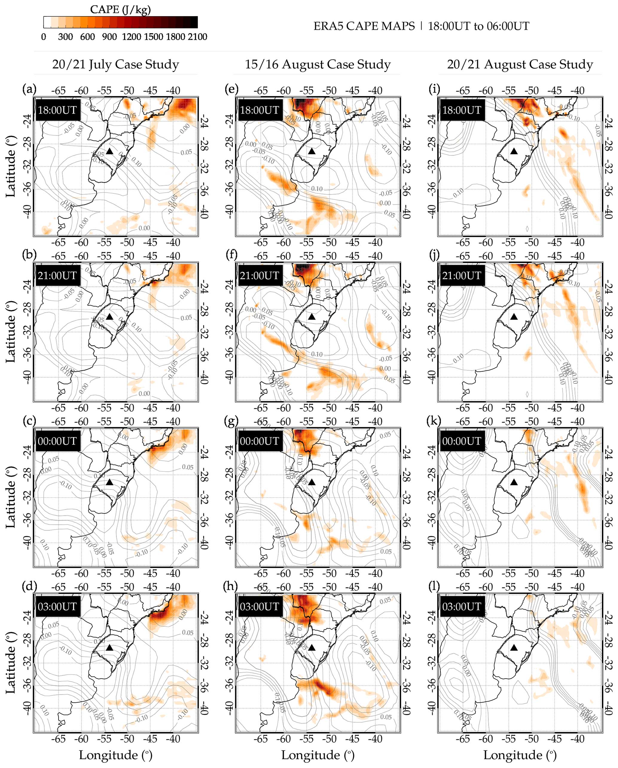
Figure 18 Spatiotemporal evolution of convective available potential energy (CAPE), with the omega (upward vertical motion of air mass) overplotted in gray contour lines.

Figures 17 and 18 present the results of coincident observations and reanalysis data used to investigate the state of the tropospheric activity. Figure 17 clearly shows the passage of the cold fronts during the three selected case studies. For the case of 20–21 July, the cold front was moving eastward, whereas the 15–16 and 20–21 August events were moving southwestward. A close observation of the omega over the cold front showed that the region with colder temperature has negative omega at 850 hPa, which indicates a consistent ascending motion of the atmosphere (Xu et al., 2015). In the cases of 20–21 July and 15–16 August, regions with negative omega are over Uruguay and part of Argentina between 18:00 and 06:00 UT. These regions are to the south and southwest of the observation site. For the case of 20–21 August, the region of the passage of the cold front was over latitudes higher than −25° and the majority over the Atlantic Ocean. The omega with a negative sign coincides with these regions. The characteristics of the cold fronts are further affirmed using the CAPE maps (Fig. 18).

CAPE is used as an indicator of atmospheric instability, which measures the integrated work that the upward buoyancy force would perform on a given mass of air to rise vertically through the entire atmosphere (Holton and Hakim, 2012). In this work, we used CAPE further to show the state of instability of the atmosphere. Several works by researchers (e.g., Vadas et al., 2009; Xu et al., 2015; Nyassor et al., 2021) used CAPE (updraft) to infer the possibility of severe weather that can lead to overshooting and consequently GWs excitation. According to the Storm Prediction Center (SPC) of the National Oceanic and Atmospheric Administration (NOAA) (Nyassor et al., 2021), CAPE is classified as marginally unstable when 0 ≤ CAPE ≤ 1000, moderately unstable when 1000 ≤ CAPE ≤ 2500, very unstable when 2500 ≤ CAPE ≤ 4000, and extremely unstable when CAPE ≤ 4000.

The higher the value of CAPE, the greater the possibility of the formation of severe weather and also the higher the maximum updraft velocity that may lead to overshooting of the tropopause and thereby exciting GWs. In the case studies considered in this work, the values of the CAPE were very low, especially in the regions indicated by the ray tracing to be the possible source location of the QMGWs, as shown in Fig. 18. This, therefore, strengthens the result in Figs. 10 and 13 that the source mechanism of the GWs observed in these case studies is not through the mechanical oscillator (overshooting) effect.

The observed CTBT map did not show overshooting, implying that the clouds did not extend too high to the upper troposphere. To further confirm this, the vertical column of the cloud (see Fig. A1 in Appendix A) was analyzed. For the case study of 20–21 July, there was no observation of CloudSat. On the other hand, there were observations during the case studies of 15–16 and 20–21 August, where CloudSat passed right through the region of negative omega (see Figs. 17 and 18). Clearly, Fig. A1 showed the presence of only low-level clouds. Another piece of evidence to show that the three case studies in this work were not excited through the mechanical oscillator (overshooting) mechanism is the vertical profile of omega at fixed longitude and varying latitude, as shown in Fig. A2. The vertical profiles of the cloud and omega are specifically presented to further affirm the result of the cold front (Fig. 17) and CAPE (Fig. 18) maps, which indicate that no overshooting took place, despite being clearly depicted in Figs. 10 and 13. For details on the vertical profiles of the clouds and omega, see Appendix A.

All this evidence clearly shows that the QMGW events selected for the three case studies are not excited through the mechanical oscillator effect mechanism of convection. However, other mechanisms associated with a cold front can excite these waves. We now investigate this possible mechanism.

7.2 Wind shear

Cold fronts are known to be characterized by temperature field but also by pressure, wind speed, and the direction that precede and succeed its passage. Pressure zones, wind speed, and direction can also identify cold fronts. The characteristics of the wind are such that a sudden change in wind direction commonly occurs with the passage of a cold front. According to Van Den Broeke (2022), before the arrival of the front, winds ahead of the front (in the warmer air mass) are typically from the south-southwest. Still, the winds usually shift to the west-northwest (in the colder air mass) after the front passage. These case studies, however, occurred during the winter season when strong wind shear and jet streams are prominent.

Strong wind shear in the upper troposphere–lower stratosphere are responsible for generating tropopause shear layers, which generate local turbulence and consequently can lead to mixing air between these two different layers (Kaluza et al., 2021). This mixing air contributes to the emergence of dynamic instabilities that conduct waves to overturn, followed by the turbulent flow breakdown in this transition region. This approach has been discussed in the context of clear-air turbulence (CAT) since 1970 (e.g., Shapiro, 1976, 1978). Recently, a midlatitude cyclone was simulated using the high-resolution numerical model in which much turbulence were reported. This information highlights the importance of the tropospheric jet streak, wind speed, and shear enhancement within upper-tropospheric outflow with the occurrence of CAT and the generation of gravity waves on different scales (Trier et al., 2020). A jet streak is a section of the overall jet stream in which winds are greater along the jet core flow than in other parts of the jet stream.

Following this approach, the horizontal winds at 200 hPa are analyzed for each event in these selected case studies (Fig. 19). The horizontal wind speed (contour plot) and direction (overplotted vector in red arrows) at 200 hPa of the case studies of 20–21 July, 15–16 August, and 20–21 August are presented in panels (a), (b), and (c) of Fig. 19, respectively. These winds are obtained from the National Centers for Environmental Prediction (NCEP) (Kalnay et al., 1996). The sub-panels labeled (i) and (ii) represent the wind speeds and directions at 18:00 UT on the previous day and 06:00 UT on the next day of each case study, with their respective speed in the color bar.

It is important to note that these events occurred during the winter when the polar jet stream (wind ∼ 60 m s⁻¹) is generally displaced southward, as observed in these three events. Bertin et al. (1978) showed many possible source mechanisms of gravity waves observed in the mesosphere that appear to be closely related to tropospheric jet streams, principally on the polar side of jets. Mastrantonio et al. (1976) showed that the gravity waves generated by tropospheric jet streams may have the ability to propagate vertically to the upper atmosphere, such as the ionosphere (Mastrantonio et al., 1976). Using two synchronized automated digital cameras at Krasnogorsk and Obninsk, located near Moscow, Russia, Dalin et al. (2015) demonstrated that a particular transient isolated gravity wave in the summer mesopause is associated with the passage of an occluded front or the point of occlusion or possibly both. The source mechanism of the wave generation, according to Dalin et al. (2015), was likely due to strong horizontal wind shear at about 5 km altitude. Similarly, Dalin et al. (2016) illustrated that gravity waves, observed in the summer mesopause, were associated with the upper-tropospheric jet stream at altitudes 8–10 km.

Figure 19 Horizontal wind at 18:00 and 06:00 UT on 20–21 July 2017 (a.i–ii), 15–16 August 2017 (b.i–ii), and 20–21 August 2017 (c.i–ii).

Figure 19a shows a strong and clear bifurcation of the strong wind flow close to longitude −60°, coinciding with the source location of the gravity waves. This bifurcation was persistent with strong wind flow throughout the 12 h, suggesting a constant emission of the gravity waves in this region. It can be observed that the wind was toward the northeasterly direction at 18:00 UT on 20 July and 06:00 UT on 21 July. The propagation direction of the wave during this case study was northeastward at the beginning of the observation on 20 July 2017.

Now we investigate the source of the QMGWs of the 15–16 August case study. Similar to the case study of 20–21 July, Fig. 19b shows a confluence of the strong wind flow from the north and southwest towards the southeasterly direction over the region. This unidirectional wind flow may suggest a persistent and unidirectional emission of gravity waves throughout the 12 h. Close to the observation site, the omega was upward where the clouds were formed (see Fig. 17e–h). In Fig. A2b, omega extends almost throughout the altitude ranges considered in the sub-panels labeled (i) and (ii).

Finally, similar to Fig. 19b, a confluence of the strong wind flows from the northwest and south to the southeast direction close to the region of study is observed in Fig. 19c. The wind considered to be associated with the source mechanism of the case study of the 20–21 August QMGWs presented a different characteristic. Figure 11c–d shows that the two wavelength groups of these QMGWs have different propagation directions. The 30–40 and 40–50 km wavelengths had no well-defined propagation direction. The ray tracing, on the other hand, showed that only three of the waves were generated in the troposphere. The remaining waves reflected above ∼ 60 km. The ray path of the wave that reached the troposphere revealed that these waves were generated in the southwestern part of the observation site. In the troposphere, Fig. 17i–l showed that the cold front extends from the northeastern, eastern, and southwestern parts of the observation site. This system is quite distant from the observation site. Considering the propagation direction of the waves, there is no way these waves can be excited by this system. According to Pramitha et al. (2016), wind shear can excite GWs, so considering the propagation of this wave, wind shear is most likely the source of this wave.

The vertical profiles of the omega (Fig. A2), zonal wind (Fig. 20), and wind shear (Fig. 21) at fixed longitudes are analyzed to identify the main characteristics of the vertical position of the jet streams close to the observation site. The fixed longitudes (Figs. A2 and 20) in case study 1 are 60 and 65° W (panels a), in case study 2 are 50 and 60° W (panels b), and in case study 3 are 50 and 40° W (panels c), respectively. The fixed longitudes for Fig. 21 are 62.5° W (case study 1; panel a), 55° W (case study 2; panel b), and 45° W (case study 3; panel c), respectively.

The vertical positions of the jet streams are close to 400 hPa for these three case studies, due to their occurrences during the winter season. The bifurcation (indicated by the dashed–dotted rectangle) of the wind flow is easily identified in panel (a) for the first case study, while the confluences (indicated by the dashed–dotted rectangle) of the wind flows are observed in case studies 2 (panels b) and 3 (panels c). The latitude with strong jet stream signatures corresponds to the latitude of the observation site.

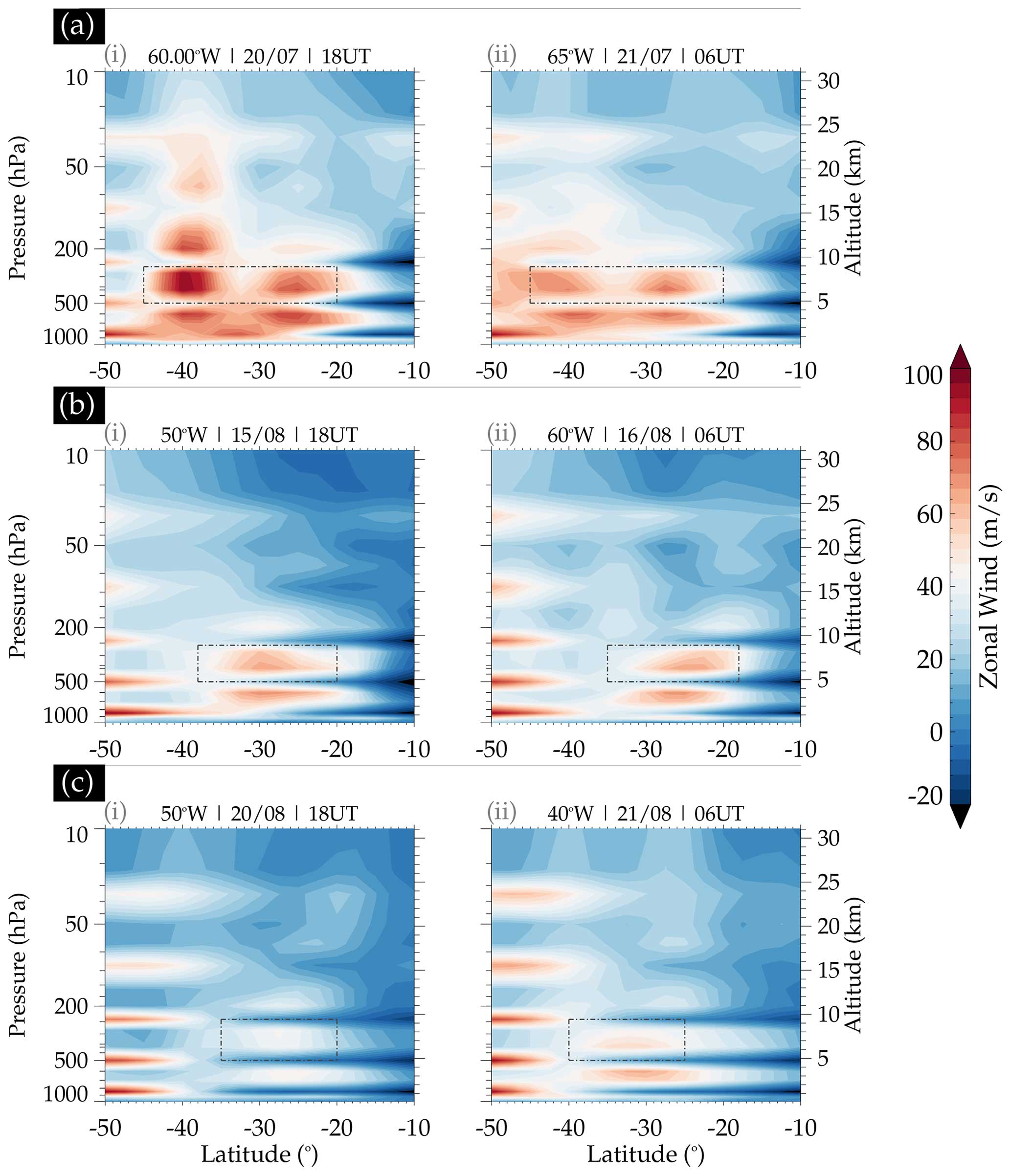
Figure 20 Zonal wind vertical profile at the fixed longitude stated in the upper-left corner of the sub-panels labeled (i) and (ii), and varying latitudes are presented. The sub-panels labeled (i) show the NCEP zonal wind profile at 18:00 UT on (a) 20 July, (b) 15 August and (c) 20 August. In the sub-panels labeled (ii), the profile at 06:00 UT on (a) 21 July, (b) 16 August and (c) 21 August is shown.

The vertical profiles of the omega (Fig. A2) show the ascendant motions slightly below the jet stream and descendant motions in the jet stream core, suggesting that the presence of the wind shear is close to the source region of all the events in this study. This behavior of the vertical motions may trigger the physical processes responsible for generating the turbulence close to the tropopause, which can lead to gravity wave generation. The excited waves can propagate vertically to the upper atmosphere (see Mastrantonio et al., 1976, and Bertin et al., 1978). Also, the vertical profile of the wind shear presented in Fig. 21, estimated using horizontal wind obtained from the NCEP Global Forecast System (GFS) data, is studied.

Figure 21 Vertical profile of vertical wind shear at 00:00 UT on 21 July 2017 (a), 16 August 2017 (b), and 21 August 2017 (c). The color bar shows the scale of the wind shear.

The vertical profiles of the wind shear in Fig. 21 show values greater than $\mathrm{15}\times {\mathrm{10}}^{-\mathrm{3}}$ s⁻¹ close to the center of the jet streams (dashed–dotted dark gray rectangles), where the vertical displacement of the wind shear (dark gray rows) is observed in these three events. This indicates the occurrence of turbulence close to the jet stream region with the vertical upward extension. These values are in accordance with the literature, which indicates the occurrence of CAT in the troposphere (Menegardo-Souza et al., 2022). The vertical extension of wind shear can generate gravity waves capable of propagating vertically.

Several possible source mechanisms for generating the selected case studies have been presented in the previous section. However, some of these mechanisms cannot be responsible for the excitation of these events because they did not meet the necessary requisite conditions. For instance, the overshooting mechanism is not possible based on the inability of the convective system to overshoot. This is not obvious, since the selected cases were observed in winter, where deep convection is less prominent. On the other hand, jet streams associated with the cold front have been strong before, during, and after these events.

Jet streams are relatively narrow bands of strong wind blowing from west to east in the upper troposphere–lower stratosphere (UTLS). As the jet stream changes in intensity and location, the strength and motion of air masses are affected, and when the air masses converge, they form fronts. When colder air mass replaces warmer air mass, colder fronts are formed. This is the exact condition in the lower atmosphere during these events. As a result, further analysis was conducted on the jet stream to establish a relationship between the jet streams, namely the GW excitation mechanism and the observed GWs.

GWs observed in the upper mesosphere can be excited by jet streams in the lower atmosphere (Song, 2021, and references therein). From the above analyses, it is clear that the activities of jet streams may be the mechanism that led to the emission of the observed QMGWs in the selected case studies.

8 Conclusions

In this study, 209 QMGWs were observed from April 2017 to April 2022, among which ray-tracing results showed that 184 were excited in the troposphere, whereas the remaining 25 were reflected above. Statistically, it was observed that among the 64 wave packets from which the 209 QMGWs were obtained, there was a high occurrence of QMGWs in August, followed by July, with the least occurrence in May. Estimates of wave parameters after applying spectral analysis revealed that the horizontal wavelength ranges between 10 and 55 km, with an average value of 22.50 km, periods between 0 and 80 min, and phase speeds between 0 and 100 m s⁻¹.

The propagation direction of the waves showed quite anisotropic distribution, with dominant distribution within northeast through north to northwest and east to south. These propagation directions are consistent with the ray-traced source locations and the CTBT distributions. Relating the source locations to the CTBT locations, it was observed that most of the waves were not excited by convection activity, as revealed by the seasonal distribution of CTBT. The duration of the QMGWs in OH images lasted between 2 and 10 h, with the 2 h duration having the highest number of QMGW events, whereas the 10 h duration had the least QMGW events. The propagation time of the waves from the OH emission layer altitude to the troposphere ranges from 0 to 9 h. Besides the total QMGW cases presented, three QMGW events on 20–21 July, 15–16 August, and 20–21 August 2017 were selected for case studies. The selected waves were grouped according to their horizontal wavelengths, after which their propagation dynamics were studied relative to their source.

The propagation directions of the case study of 20–21 July 2017 QMGWs showed that the directions of the waves varied from the northwest through north to southwest. However, the ray-tracing result showed that, except for one wave that reached the troposphere, the rest of the waves reflected above ∼ 60 km. This is an indication of the possibility of ducting or reflection. To further investigate the details of this possibility, propagation characteristics due to the background field were conducted. It was found that the duct enhanced the longer propagation of this event and also the changing propagation direction. The source of these case studies was most likely jet streams. Similarly, the sources of the 15–16 and 20–21 August case studies are also most possibly due to the jet stream. Contrarily, most of the ray paths of these waves reached the troposphere, signifying that these waves were excited in the troposphere. In the case of the 20–21 August case studies, about seven waves reflected above 60 km.

In conclusion, the current study presents statistical evidence of the occurrence of QMGWs. Their occurrences were further investigated in detail, using the seasonal distribution of the propagation directions in relation to the seasonal CTBT distributions in space indicated by the ray tracing to be the possible source location. Due to the peculiar characteristics of the three case studies and their occurrence in the winter month, they were chosen for further detailed studies. These case studies were ducted; as a result, they could propagate longer distances with quasi-horizontal wavelength for a long time. The sources of these case studies were not related to convective activity but to jet streams.

Appendix A

A1 CloudSat 2B-GEOPROF vertical profile of the cloud

The level 2B GEOPROF R04 and R05 products of CloudSat determine levels in the vertical column sampled by CloudSat that contain significant radar echo from hydrometeors and then provides the radar reflectivity factor. GEOPROF also includes a product that estimates the expected gaseous absorption loss for the observed reflectivity, which is dependent on water vapor fields from the European Centre for Medium-Range Weather Forecasts (ECMWF). The Moderate Resolution Imaging Spectroradiometer (MODIS) cloud fraction from MOD35 associated with the radar surface footprint and several other flags indicates the homogeneity of the MODIS data and the quality of the CloudSat data. Details on the GEOPROF algorithms and structure of the HDF-EOS (Hierarchical Data Format – Earth Observing System) output files can be found in Marchand et al. (2008) and the level 2 GEOPROF Product Process, Description, and Interface Control Document.

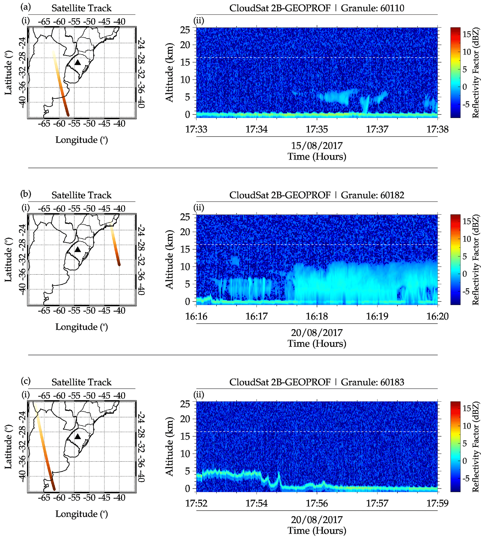
Figure A1 CloudSat 2B GEOPROF vertical profile of the cloud during the (a) 15–16 August 2017 and (b, c) 20–21 August 2017 QMGWs case studies. The sub-panel labeled (i) is the satellite track, and the sub-panel labeled (ii) is the vertical profile of the cloud.

Using the level 2B GEOPROF R04 and R05, the vertical column of the clouds and the CloudSat track were obtained. In Fig. A1, the track of the satellite and the cloud vertical column are shown for the cases of 15–16 August (panel a) and 20–21 August 2017 (panels b and c). The satellite did not pass during the July 20–21 event; hence, no plot is presented for this day. In Fig. A1, the sub-panel labeled (i) represents the track of the CloudSat, while the sub-panel labeled (ii) shows the vertical column of the cloud with time. In the sub-panel labeled (ii), the horizontal dashed lines depict the radiosonde tropopause altitude at 00:00 UT on 16 and 21 August. The color bar shows the scale of the radar reflectivity factor (dBZ).

Between 17:33 and 17:38 UT on 15 August (Fig. A1b), the vertical column of cloud for the nearby track of sounding is presented. This time is earlier than the time interval for the cold front and CAPE maps. However, the figure is presented to prove the existence of the cloud, but only a low-level cloud between 17:35 and 17:38 UT was observed.

Before the case study of 20–21 August, CloudSat made two passages, one between 16:16–16:20 UT (Fig. A1b.ii), with the track shown in Fig. A1b in the sub-panel labeled (i). The satellite passed through the location of the cold front, which also corresponded to the negative omega region. A well-defined profile of the vertical column of the cloud was captured, since the satellite passes right through the middle of the cloud within this time range. Even though the CTBT maps showed cold cloud-top temperatures (see panels i, j, k, and l of Fig. 17), the vertical column of clouds extended up to about 12 km (see Fig. A1), which is about 4 km lower than the tropopause height. This, furthermore, shows that no overshooting occurred; hence, this source mechanism cannot be responsible for generating the GWs of this case study. The second satellite track shown in Fig. A1c in the sub-panel labeled (i) between 17:52 and 17:59 UT could not capture any cloud profile (see Fig. A1c in the sub-panel labeled (i)) because there was no cloud present at that time. At 18:00 UT, a system of clouds was seen progressing from the southwestern part towards the northeast but dissipated as time progressed. Without clouds near the source location of the QMGWs in this case study (Fig. 12d), the implication is that other mechanisms will be the source of this case study.

A2 Vertical profile of omega (ω)

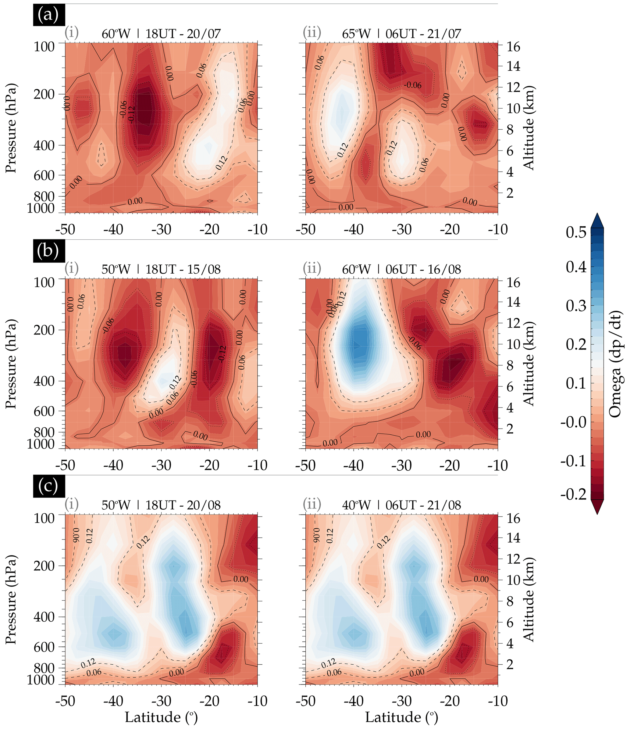
Figure A2 Vertical profile of omega (ω) at 18:00 and 06:00 UT on 20–21 July 2017 (a.i–ii), 15–16 August 2017 (b.i–ii), and 20–21 August 2017 (c.i–ii).

Figure A2 presents the vertical profiles of omega for the case studies of 20–21 July, 15–16 August, and 20–21 August. In panels (a), (b), and (c), the plot of omega with altitude (units in hPa and km) for the three case studies is presented. The omega used in these plots was obtained at varying latitudes of −50 to −10° S and fixed longitudes at 60° W (the sub-panel labeled (i)) and 65° W (the sub-panel labeled (ii)) for panel (a); 50° W (the sub-panel labeled (i)) and 60° W (the sub-panel labeled (ii)) for panel (b); and 50° W (the sub-panel labeled (i)) and 40° W (the sub-panel labeled (ii)) in panel (c). The altitude in kilometers for all panels corresponding to the pressure levels in hectopascals (on the left side of the sub-panel labeled (i)) is on the right side of the sub-panel labeled (ii).

From the omega vertical profiles of the three case studies at a fixed longitude and varying latitudes, we observed negative omega in the 20–21 July event, extending from 0 to the tropopause for panel (a) with the sub-panel labeled (i) of Fig. A2. For panel (a) with the sub-panel labeled (ii), at 65.00° W, −50 to −10° S, the negative omega extended almost throughout the entire pressure/altitude range considered. The omega ascended almost throughout the profile for the 15–16 August case study. However, a descending region from 200 to 600 hPa and −35 to 25° S in panel (b) with the sub-panel labeled (i) and −45 to 30° S in panel (b) with the sub-panel labeled (ii). A different omega distribution was observed in the case of 20–21 August (i.e., Fig. A2). The positive omega (signifying downward motion of air) dominates the altitude range from 3 to ∼ 15 km and between −50 and −20° S. Beyond −20° S, omega was ascending. Figure A2 shows that, even with the upward movement of the air mass, its effect did not lead to the formation of clouds and eventually to the excitation of GWs. The omega vertical profile further affirms the previous evidence that these three QMGW events are not excited through overshooting. However, omega is used not only as an indicator for cloud formation but also for vertical wind shear.