the Creative Commons Attribution 4.0 License.
the Creative Commons Attribution 4.0 License.
 | 30 Apr 2024
Analytical approximation of the definite Chapman integral for arbitrary zenith angles
Dongxiao Yue
This study presents an analytical approximation of the definite Chapman integral, applicable to any zenith angle and finite integration limits. The author also presents the asymptotic expression for the definite Chapman integral, which enables an accurate and efficient implementation free of numerical overflows. The maximum relative error in our analytical solution is below 0.5 %.
- Article
(499 KB) - Full-text XML
- BibTeX
- EndNote


The Chapman function, a specific improper integral, has wide application in diverse fields of study (Chapman, 1931, 1953), including but not limited to radiative transfer theory, aeronomy, and atmospheric absorption and scattering in general (Bauer and Lammer, 2004; Brasseur and Solomon, 2005; Schunk and Nagy, 2009; Grieder, 2010; Engel, 2018). It represents the integration of an exponentially varying density along a slanted path within spherical geometry. In computing atmospheric attenuation and scattering over finite distances, the definite form of this integral becomes essential. Several researchers (Green and Barnum, 1963; Fitzmaurice, 1964; Swider and Gardner, 1969; Titheridge, 1988; Kocifaj, 1996; Huestis, 2001) have proposed various analytical approximations of the Chapman function. A comprehensive review and an improvement of these approximations were recently offered by Vasylyev (2021). Nonetheless, a straightforward solution applicable to arbitrary path angles and finite integration limits remains elusive. Our work addresses this gap by offering a comprehensive solution for the definite Chapman integral, ensuring precision over finite distances and aligning with the Chapman function at infinite limits.
Boltzmann's distribution, at a constant temperature T, describes the exponential decrease in air molecule density with altitude h, as follows:
Here, m denotes the mass of a single molecule, g the gravitational acceleration, kB the Boltzmann constant and T the absolute temperature. On a planet with radius R, the assumption of constant g is valid only when h≪R.
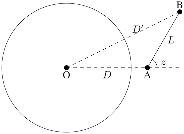
Considering a planet of radius R, as shown in Fig. 1, starting from point A in the atmosphere at distance D from the center, along a path at angle z from the zenith, the integral of density along the path A–B is proportional to
where . The H in the exponent is termed the scale height. Since the integral is performed in the atmosphere, the exponent is always negative, and the integral is well defined and is smaller than L.
Given the average density ρ of the planet, gravitational acceleration near the surface (h≪R) can be approximated as , G being the gravitational constant. For an effective molecular mass m, the scale height H can be expressed as
Using a molecular weight W, and substituting standard values for (in MKS units) and the ideal gas constant 8.31 J mol−1 K−1, we arrive at . For Earth, with kg m−3 and m, at a temperature of 300 K and molecular weight of 30, H is calculated to be approximately 8.5×10³ m. More pertinent to the Chapman integral is the ratio , which for Earth is around 700. Generally, the ratio can be estimated as
For rocky planets larger than 1000 km in radius and with similar density to Earth, the ratio is typically in the hundreds. This implies a relatively thin atmospheric layer compared to the planet's size, allowing the assumption of constant gravity as used in Eq. (6). We therefore propose changing the integration over travel distance in the atmosphere to one over the change in the radial distance.
Defining , , , and , we reformulate integral I as
Observing that , we define the term in square brackets as the definite Chapman integral, i.e., the Chapman integral with finite integration limits.
Specifically, we identify
where Ch(λ,z) is the Chapman function as defined in Chapman (1931).
To perform the integral Cd in Eq. (6), we make the following change of variable:
Restricting z to , there is a one-to-one mapping between t and u. Using the relationship , the integral is transformed to
Geometrically, referring to Fig. 1, the upper limit of the integral , denoting the variation in radial distance at the boundary of integration, normalized by the initial distance. Given that the atmospheric thickness of a planet is significantly less than its radius, the upper limit y is much smaller than 1 (). With the range of z confined to , sin z is non-negative, this permits the approximation . With this simplification, the above integral can be approximated as follows:
Since λ is large, the main contribution to the integral comes from small u values. Moreover, the assumption of constant gravity in deriving the exponential drop of density is valid only when the atmosphere depth is much smaller than planet radius. These considerations further justify our approximation.
By another change of variable, , then integrate by parts, the integral can be analytically expressed using the erfc(t) function (complementary error function), which is defined as .
To simplify the expression of our result, we define function for ,
and define function as
The definite Chapman integral is found to be
where y is defined by Eq. (8); i.e., . Geometrically, , DB being the distance from the end point to the center of the planet.
To study the behavior of , we examine its first derivative:
Since is always positive, increases monotonically with y. Moreover, due to the factor e−λy, the derivative quickly approaches 0 at λy≫1. This indicates that the integral's primary contribution comes from within a few multiples of the scale height, while the contribution from higher altitudes becomes inconsequential. For instance,with λ=500, plateaus around y≈0.02. Consequently, serves as an excellent approximation for the Chapman function, despite the latter having the integration limit extended to infinity. Our results (Eqs. 11–13) agree with the approximate formulas tabulated in Vasylyev (2021) when evaluated under appropriate limits.
Our result is an analytical solution for the definite Chapman integral applicable to zenith angles z restricted to the range . In this context, y must be positive. However, our solution can be easily extended to situations where , involving a decrease in radial distance along the integration path. In the simplest scenario, reversing the start and end points of the integration ensures that the zenith angle is at the starting point. For such cases, it is merely a matter of redefining D and z based on the new starting point.
Figure 2 depicts a more intricate scenario, where the zenith angles at both integration ends exceed .
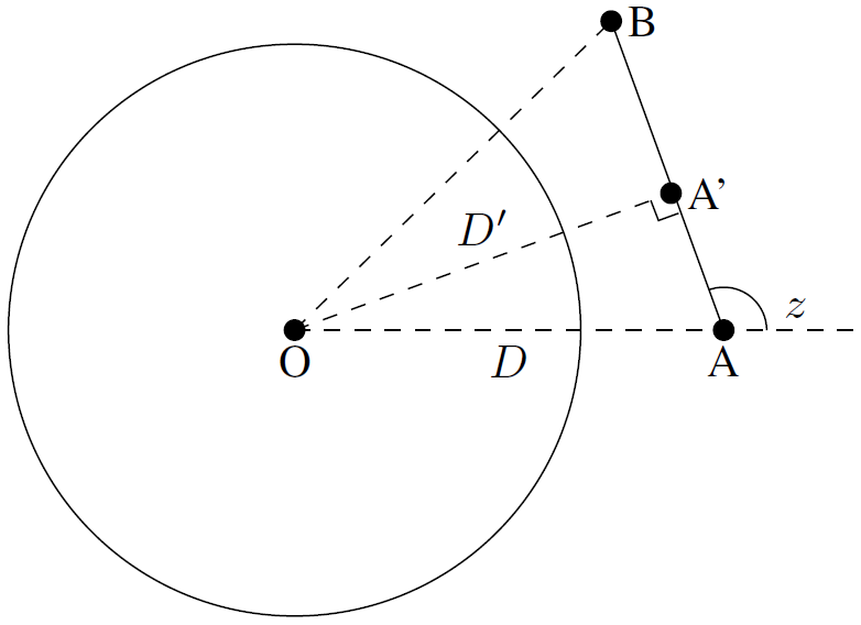
Figure 2Illustration of the density integral from point A to B, with zenith angles greater than at both endpoints. The integral is divided into two parts at point A′, enabling the application of the Y function.
To adapt the function to the case illustrated in Fig. 2, the approach involves altering the integration's starting point. This is achieved by drawing a perpendicular line from the center of the planet to the line AB and taking the intersection point A′ as the new starting point. The Y function is then applied to two segments, from A′ to A and from A′ to B, both with a zenith angle of .
With this change of the starting point, let , , and :

Given that λ is significantly greater than 1, the erfc function values in Eq. (11) rapidly converge to 0 at both limits for most z values (for instance, ). Simultaneously, the exponential factor of the second term inside the equation's brackets becomes exceedingly large for most z values. As previously mentioned, the original integral remains well defined and is smaller than the length of integration. Therefore, Eq. (12) is dependent on the near cancellation of erfc values at the integration limits:
For high values of λ, attempting a direct numerical calculation using Eqs. (11)–(12) could lead to overflow issues with the exponential term and imprecise results in the Δ term, due to the limitations in floating-point precision. It is crucial to analytically neutralize the positive exponent in the second term of Eq. (11). When , by retaining only the principal term in the asymptotic expansion of erfc(x), namely , we can simplify the Δ expression:
Using the above result, at large λ(1−sin z), Eq. (13) becomes
and when λy≫1, the exponentially small terms in above can be dropped. The formula is reduced to the well-known result in the limiting case.
It is important to observe that this approximation holds true only when , and cos z is non-zero at this limit. This indicates that for small zenith angles, the atmospheric curvature can be disregarded, and the optical depth calculations can be based simply on the length of the slanted path.
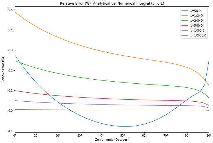
The sole approximation in our derivation was made in Eq. (10). Our analytical results, spanning Eqs. (11)–(15), are valid for any zenith angle, including . To evaluate our solution, we compared the analytical results from (Eqs. 11–12) with direct numerical integration of the original integral in Eq. (6), across a range of λ values and zenith angles within . Then we plotted the relative error of our analytical solution, calculated as the discrepancy between the analytical and numerical results, normalized by the numerical integral. The full evaluation is demonstrated in the GitHub repository (Yue, 2024). The key resulting plots are presented in Figs. 3 and 4.
Our numerical evaluations revealed that the maximum relative error in the analytical solution remained under 0.5 % for λ values ranging from 50 to 10 000. Furthermore, the asymptotic approximation in Eq. (18) demonstrates high accuracy, with the maximum relative error of less than 1 % when it is applied at . Even when the asymptotic approximation is switched on at , the relative error stayed below 5 %.
Additionally, we assessed our analytical results at an upper limit of y=0.1 for λ values between 50 and 10 000, juxtaposing them with the numerical values of the Chapman function. The comparisons indicated that they are within 0.5 % of each other.
In summary, our study provides a comprehensive analytical solution for the definite Chapman integral, applicable to any zenith angle and realistic λ values. The accuracy of our solution has been rigorously tested against direct numerical integrations, demonstrating a high degree of precision with relative errors consistently below 0.5 %. The solution is notable in its simplicity and versatility. This work paves the way for more efficient and accurate atmospheric effect analyses and related studies.
The Python code for evaluating the analytical approximation of the definite Chapman is available online on GitHub https://github.com/ydx2021/yuedx/, last access: 22 December 2023 (Yue, 2024).
The sole author, DY, PhD, conducted all aspects of the research, including conceptualization, calculation, analysis, coding, writing, and reviewing, and is responsible for the entire paper.
The author has declared that there are no competing interests.
Publisher’s note: Copernicus Publications remains neutral with regard to jurisdictional claims made in the text, published maps, institutional affiliations, or any other geographical representation in this paper. While Copernicus Publications makes every effort to include appropriate place names, the final responsibility lies with the authors.
This paper was edited by John Plane and reviewed by two anonymous referees.
Bauer, S. J. and Lammer, H.: Radiation and Particle Environments from Stellar and Cosmic Sources, in: Planetary Aeronomy, Phys. Earth Space Env., Springer, Berlin, Heidelberg, 3–30, https://doi.org/10.1007/978-3-662-09362-7_2, 2004. a
Brasseur, G. and Solomon, S.: Aeronomy of the Middle Atmosphere, Atmospheric and Oceanographic Sciences Library, Vol. 32, Springer, Boulder, Colorado, https://doi.org/10.1007/1-4020-3824-0_4, 2005. a
Chapman, S.: The absorption and dissociative or ionizing effect of monochromatic radiation in an atmosphere on a rotating earth part II. Grazing incidence, Proc. Phys. Soc., 43, 483–501, https://doi.org/10.1088/0959-5309/43/5/302, 1931. a, b
Chapman, S.: Note on the grazing-incidence integral ch(x,χ) for monochromatic absorption in an exponential atmosphere, Proc. Phys. Soc. B, 66, 710–712, https://doi.org/10.1088/0370-1301/66/8/411, 1953. a
Engel, W.: GPU Pro 360 Guide to Rendering, 1st Edn., A. K. Peters, Ltd., USA, ISBN 0815365519, 2018. a
Fitzmaurice, J. A.: Simplification of the Chapman function for atmospheric attenuation, Appl. Opt., 3, 640–640, https://doi.org/10.1364/AO.3.000640, 1964. a
Green, A. E. S. and Barnum, L.: Note on a simple approximation to the chapman function, Space Sci. Lab., General Dynamics/Astronautics, San Diego, California, 1963. a
Green, A. E. S., Lindenmeyer, C. S., and Griggs, M.: Molecular absorption in planetary atmospheres, J. Geophys. Res., 69, 493–504, https://doi.org/10.1029/JZ069i003p00493, 1964.
Grieder, P. K. F.: Extensive Air Showers: High Energy Phenomena and Astrophysical Aspects – A Tutorial, Reference Manual and Data Book, 1st Edn., Springer, Berlin, Heidelberg, https://doi.org/10.1007/978-3-540-76941-5, 2010. a
Huestis, D. L.: Accurate evaluation of the Chapman function for atmospheric attenuation, J. Quant. Spectrosc. Ra., 69, 709–721, https://doi.org/10.1016/S0022-4073(00)00107-2, 2001. a
Kocifaj, M.: Optical air mass and refraction in a Rayleigh atmosphere, Contrib. Astron. Obs. Skalnate Pleso., 26, 23–30, 1996. a
Schunk, R. and Nagy, A.: Ionospheres: Physics, Plasma Physics, and Chemistry, 2nd Edn., Cambridge Atmospheric and Space Science Series, Cambridge University Press, ISBN 9780511635342, https://doi.org/10.1017/CBO9780511635342, 2009. a
Swider, W. and Gardner, M. E.: On the Accuracy of Chapman Function Approximations, Appl. Opt., 8, p. 725, https://doi.org/10.1364/AO.8.000725, 1969. a
Titheridge, J. E.: An approximate form for the Chapman grazing incidence function, J. Atmos. Terr. Phys., 50, 699–701, https://doi.org/10.1016/0021-9169(88)90033-5, 1988. a
Vasylyev, D.: Accurate analytic approximation for the Chapman grazing incidence function, Earth Planet. Space, 73, 112, https://doi.org/10.1186/s40623-021-01435-y, 2021. a, b
Yue, D.: Numerical Validation of the Analytical Approximation to the Definite Chapman Integral, Zenodo [data set and code], https://doi.org/10.5281/zenodo.11075017, 2024. a, b