Air mass transport to the tropical western Pacific troposphere inferred from ozone and relative humidity balloon observations above Palau

The transport history of tropospheric air masses above the tropical western Pacific (TWP) is reflected by the local ozone and relative humidity (RH) characteristics. In boreal winter, the TWP is the main global entry point for air masses into the stratosphere and therefore a key region of atmospheric chemistry and dynamics. Our study aims to identify air masses with different pathways to the TWP using ozone and radio soundings from Palau from 2016–2019. Supported by backward trajectory calculations, we found five different types of air masses. We further defined locally controlled ozone and RH background profiles based on monthly statistics and analyzed corresponding anomalies in the 5–10 km altitude range. Our results show a bimodality in RH anomalies. Humid and ozone-poor background air masses are of local or Pacific convective origin and occur year-round, but they dominate from August until October. Anomalously dry and ozone-rich air masses indicate a non-local origin in tropical Asia and are transported to the TWP via an anticyclonic route, mostly from February to April. The geographic location of origin suggests anthropogenic pollution or biomass burning as a cause for ozone production. We propose large-scale descent within the tropical troposphere and radiative cooling in connection with the Hadley circulation as being responsible for the dehydration during transport. The trajectory analysis revealed no indication of a stratospheric influence. Our study thus presents a valuable contribution to the discussion about anomalous layers of dry ozone-rich air observed in ozone-poor background profiles in the TWP.

1 Introduction

The tropical western Pacific (TWP), an area extending from the Maritime Continent to the International Date Line, is considered the major air mass transport pathway from the troposphere to the stratosphere during boreal winter (e.g., Newell and Gould-Stewart, 1981; Fueglistaler et al., 2004; Krüger et al., 2008). Air masses entering the stratosphere largely originate in the local TWP boundary layer and free troposphere (Rex et al., 2014). Thus, the local tropospheric air composition has a key impact on concentrations of various chemical species within the global stratosphere, even up to a potential impact on polar ozone depletion.

Understanding (1) the variability of composition and transport of air masses to this region as well as (2) the unique air chemistry are therefore of great relevance. The monitoring of tropospheric ozone (O₃) concentrations sheds light on both aspects.

1. O₃ is a chemical tracer for both local convective (“low” O₃ in clean, maritime air, e.g., Kley et al., 1996; Pan et al., 2015) and long-range transport processes to this region (“high” O₃ from polluted or stratospheric origin, e.g., Anderson et al., 2016; Randel et al., 2016; Tao et al., 2018).

2. The abundance of ozone is important since the hydroxyl (OH) radical essentially defines the oxidizing capacity of the local troposphere. The close coupling of O₃ and OH in the very low NO_x environment of the TWP (Levy, 1971) allows estimation of the OH abundance from O₃ and relative humidity (RH) measurements and thus an assessment of chemical lifetimes (e.g., Rex et al., 2014; Nicely et al., 2016; Bozem et al., 2017).

Major research activities focusing on tropospheric air chemistry and O₃ observations have been conducted in the wider region since the late 1980s (e.g., Pan et al., 2017 and overview in Müller, 2020). The typical tropospheric composition of the TWP has been related to the local humid, marine and pollutant-free environment, favoring O₃ destruction (e.g., Kley et al., 1996; Levy, 1971):

$$\begin{array}{}\text{(R1)}& {\displaystyle }{\mathrm{O}}_{\mathrm{3}}+h\mathit{\nu }\to {\mathrm{O}}_{\mathrm{2}}+\mathrm{O}{(}^{\mathrm{1}}\mathrm{D})(\mathit{\nu }<\mathrm{310}\mathrm{nm}),\text{(R2)}& {\displaystyle }\mathrm{O}{(}^{\mathrm{1}}\mathrm{D})+{\mathrm{H}}_{\mathrm{2}}\mathrm{O}\to \mathrm{OH}+\mathrm{OH}.\end{array}$$

Observations in the TWP found low NO_x concentrations inhibiting O₃ production and thus facilitating an O₃ loss rate via the above reactions of 3.4 % per day for the tropospheric column (Crawford et al., 1997). For boundary layer O₃ in the equatorial Pacific the efficiency of this loss mechanism results in a lifetime of around 5 d (e.g., Liu et al., 1983; Kley et al., 1997). Deep convective outflow and overturning processes lift the clean boundary layer air to the Tropical Tropopause Layer (TTL). In conjunction with a lack of in situ net O₃ production, this creates a well-mixed, humid tropospheric profile with a uniform vertical O₃ distribution (e.g., Pan et al., 2015). These typical dynamical conditions are conducive to a respective zonal wave one pattern with a persistent tropospheric O₃ minimum in the TWP in particular (e.g., Thompson et al., 2003b; Rex et al., 2014).

Many studies highlight dry intrusions of enhanced O₃ volume mixing ratios (VMR) against the humid, ozone-poor background as characteristic features of the mid-troposphere for the wider tropical Pacific (e.g., Newell et al., 1999; Stoller et al., 1999; Thouret et al., 2000; Browell et al., 2001; Oltmans et al., 2001; Hayashi et al., 2008; Pan et al., 2015; Anderson et al., 2016). The importance of these distinct, anomalous layers for local air composition and climate forcing are often acknowledged (e.g., Mapes and Zuidema, 1996; Kley et al., 1997; Yoneyama and Parsons, 1999). Their genesis, source region and impact on the local radiative budget and oxidizing capacity are, however, the subject of an ongoing debate (Anderson et al., 2016; Randel et al., 2016; Nicely et al., 2016; Tao et al., 2018). Most studies agree that they have been advected from remote regions and thus indicate a departure from dominating local conditions, i.e., an absence of the local imprint on air composition (see Anderson et al., 2016, for an overview).

A long-term monitoring of tropospheric O₃ in the TWP as a key region of stratospheric entry has yet been missing (Smit et al., 2021) but is essential to clarify the source regions of air masses and their annual and interannual variability. All relevant major research campaigns in the TWP were temporarily limited to specific seasons and years, e.g., PEM Tropics/West (Newell et al., 1996), CEPEX (Kley et al., 1996), TransBrom (Krüger and Quack, 2013; Rex et al., 2014) and CONTRAST/CAST (Pan et al., 2017; Harris et al., 2017). To fill the observational gap, the Palau Atmospheric Observatory (PAO) was established in 2015 and has since been providing an unprecedented regular balloon sounding program for O₃ and RH. It is located in the center of the warm pool on the island nation of Palau, 1000 km east of the Philippines (7.34° N, 134.47° E). The instrumental setup and meteorological conditions for the time series used in this study are introduced in more detail in a companion study by Müller et al. (2024) (cf. Müller, 2020).

The aim of this study was to examine major air mass transport processes and pathways to the TWP troposphere by using balloon-borne O₃ and RH measurements from the PAO. Based on our process understanding explained in Sect. 3.1.3, we propose five major air mass pathways to Palau resulting in distinct relations between the O₃ abundance and RH in the column of air above the TWP. The continuous 4-year ozonesonde and radiosonde time series (2016–2019) enables a seasonal analysis of the source regions, reflected mainly in the O₃ variability. We distinguished between air mass categories first using a statistical, data-based approach and performed a seasonal analysis. Lagrangian backward trajectories were then used to examine according differences in air mass origin. A potential vorticity (PV) analysis was included to investigate a possible stratospheric origin.

In the following, we first introduce the observational data (Sect. 2) and methods (Sect. 3) used to define different categories of air masses, which we relate to different pathways to Palau (Sect. 3.1.1). The main results of this study are the characterization of seasonal tropospheric air mass variability (Sect. 4.1) and the verification of our process-based understanding of air mass transport using trajectory modeling (Sect. 4.2). After a discussion (Sect. 5), we conclude (Sect. 6) that the maximum of the mid-tropospheric seasonal O₃ cycle can be associated with long-range transport mainly from potentially polluted areas in Southeast Asia. We found no evidence of transport from the extratropical stratosphere. Additional figures with more details on the full seasonal extent are given in Appendix A.

2 Data

2.1 Sondes

Our analysis is based on electrochemical concentration cell (ECC) ozonesonde and radiosonde observations from January 2016–October 2019 conducted at the PAO. Balloon-borne measurements with ECC ozonesondes (Komhyr, 1969; Smit and the ASOPOS Panel, 2014) are the most practical way to observe and continuously monitor O₃ in situ, especially at more remote sites (e.g., Thompson et al., 2019). The specific instrumentation (models SPC 6A and Vaisala RS92/41) and dataset are introduced and described in detail by Müller et al. (2024), who provide additional meteorological and climatological context for the Palau time series. While carefully following the standard operating procedures (SOP) as recommended by Smit and the ASOPOS Panel (2014), the O₃ VMR are calculated using a pressure-dependent background current correction (see Müller et al., 2024, for details). Figure 1 shows a time–height cross-section of the dataset with individual soundings marked by arrows, ozone in color-filled contours and RH observations below 30 % enclosed in hatched contours. Fortnightly measurements, mostly during midday, are complemented by one or two intensive campaigns per year. The onset of measurements in the beginning of 2016 coincides with a very strong El Niño event (e.g., Huang et al., 2016; Diallo et al., 2018). As a consequence and in compliance with acknowledged El Niño–Southern Oscillation (ENSO) indices (cf. Müller et al., 2024), data before August 2016 was disregarded in some of the following statistical seasonal analysis and will be referred to as “excluding El Niño 2016”. The 2019 El Niño episode, weaker in nature, is still included.

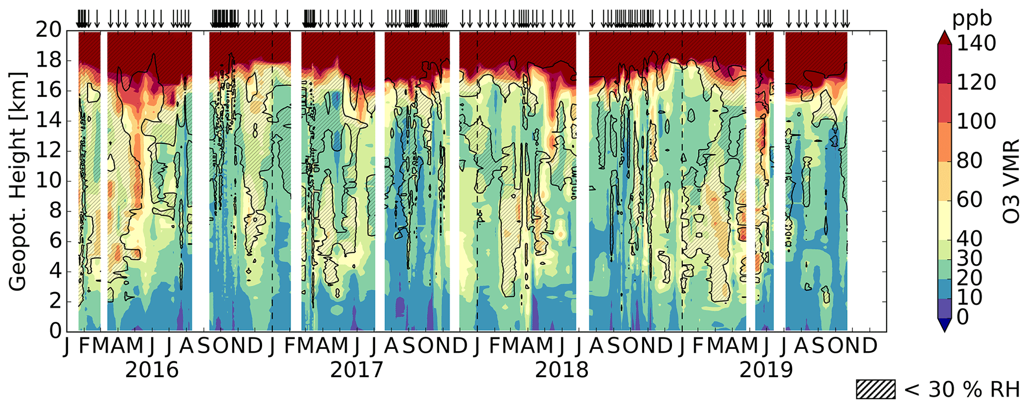
Figure 1 Tropospheric (0–20 km) time–height cross-section of O₃ VMR (in color-filled contours) and coinciding RH observations below 30 % (hatched areas enclosed in black contours) derived from PAO sounding data. Arrows on top indicate individual soundings. Data are linearly interpolated between soundings. Measurement gaps longer than 20 d are in white, beginning 7 d after or before the last or next sounding. Note the nonlinear scaling. O₃ VMR are calculated using a pressure dependent background current correction; see Müller et al. (2024) for more details.

The sparsity of the O₃ data with a sounding frequency of 0 to 11 launches per month and the resulting non-uniform distribution of the data affects the assessment of the temporal variability in our 4-year time series, which is still short for climatological studies. Details about our statistical averaging calculations can be found in Appendix B. For the trajectory analysis, the dataset was limited to 138 soundings due to missing metadata (timestamps) in some of the soundings, and the vertical profile resolution was reduced by selecting every 10th sonde reading. This dataset will be referred to as the trajectory dataset, including 13 627 individual observations in the 5–10 km altitude range.

2.2 Meteorological data

Back trajectory calculations were driven by 3D meteorological fields and diabatic heating rates from the European Centre for Medium-Range Weather Forecasts (ECMWF) Reanalysis data ERA5 (Hersbach et al., 2020) retrieved in a 1.125° × 1.125° horizontal and 3 h temporal resolution. ERA5 uses a parameterization for convection on the subgrid scale. Isolated deep convection is not captured, but the net wind flow from each grid cell is zero (Hersbach et al., 2020). While our trajectory model does not calculate convective transport, the ERA5 input therefore implicitly allows us to capture synoptic-scale convective processes.

3 Methods and analysis

The identification of differences in air mass origin by local O₃ and RH profile measurements naturally depends on the air mass definition itself. We chose air mass categories derived from statistical analysis of the two tracers, O₃ and RH, from the PAO balloon-borne time series, which reflect our process understanding in this particular location. The chemical composition of the tropospheric column above Palau is governed by the interplay of local and non-local atmospheric processes in time and space. Our air mass categories represent these differences in chemical or dynamical properties and allow attribution to local or non-local source regions. The tropospheric column of a single day can consist of a variety of air masses, sometimes visible as distinct layers within the tracer profiles.

In the following, we use O₃±RH±​​​​​​​ as a qualitative notation for air masses of low (“−”) or high (“+”) O₃ or RH, respectively (cf., e.g., Stoller et al., 1999). This leads to four qualitative categories, which we use to explain our process understanding and for comparison with previous studies (Sect. 3.1.1). The “Δ” symbol denotes quantitative air mass categories by anomalies (positive, “+”; negative, “−”) from atmospheric background profiles (i.e., close to zero anomalies, denoted as “∘”) as defined by our statistical approach. Within this anomaly space, we established a quantitative grid with nine categories with boundaries derived from the distributions of O₃ and RH anomalies, ΔO₃ and ΔRH (Sect. 4.1.3). With this approach, we particularly targeted the questions of local or non-local genesis of background air masses (ΔO₃∘ΔRH∘), which are humid and ozone-poor, and anomalously dry O₃-rich air (ΔO₃+ΔRH−) together with their respective seasonality.

3.1 Air mass definition

3.1.1 Tracers and process understanding

O₃ is a common tracer in transport studies within the TWP, with typical dynamical conditions being conducive to a tropospheric column of low O₃ VMR attributed to local air masses (e.g., Kley et al., 1996; Pan et al., 2015). Dominant marine convection leads to low NO_x concentrations and subsequently low O₃ production rates (e.g., Crawford et al., 1997; Rex et al., 2014). In this environment the HO_x-driven loss of O₃ is favored (see Reaction R2), resulting in a lifetime of about 5 d for boundary layer O₃ (e.g., Liu et al., 1983; Kley et al., 1997). The low-NO_x environment is fostered by dominating easterly winds in the annual mean and most of the troposphere (Müller et al., 2024). Most of the air reaching Palau has crossed the Pacific and has thus been cleaned of O₃ precursors from anthropogenic or other continental pollution. Palau has a hot, humid and wet climate all year, resulting in a continuously high convective activity (Gettelman and Forster, 2002; Müller et al., 2024). This persistent high convective activity creates a well-mixed profile of uniformly low O₃ VMR throughout the free troposphere, as illustrated in Fig. 2a. We refer to this as the clean state of the atmosphere or simply “background”.

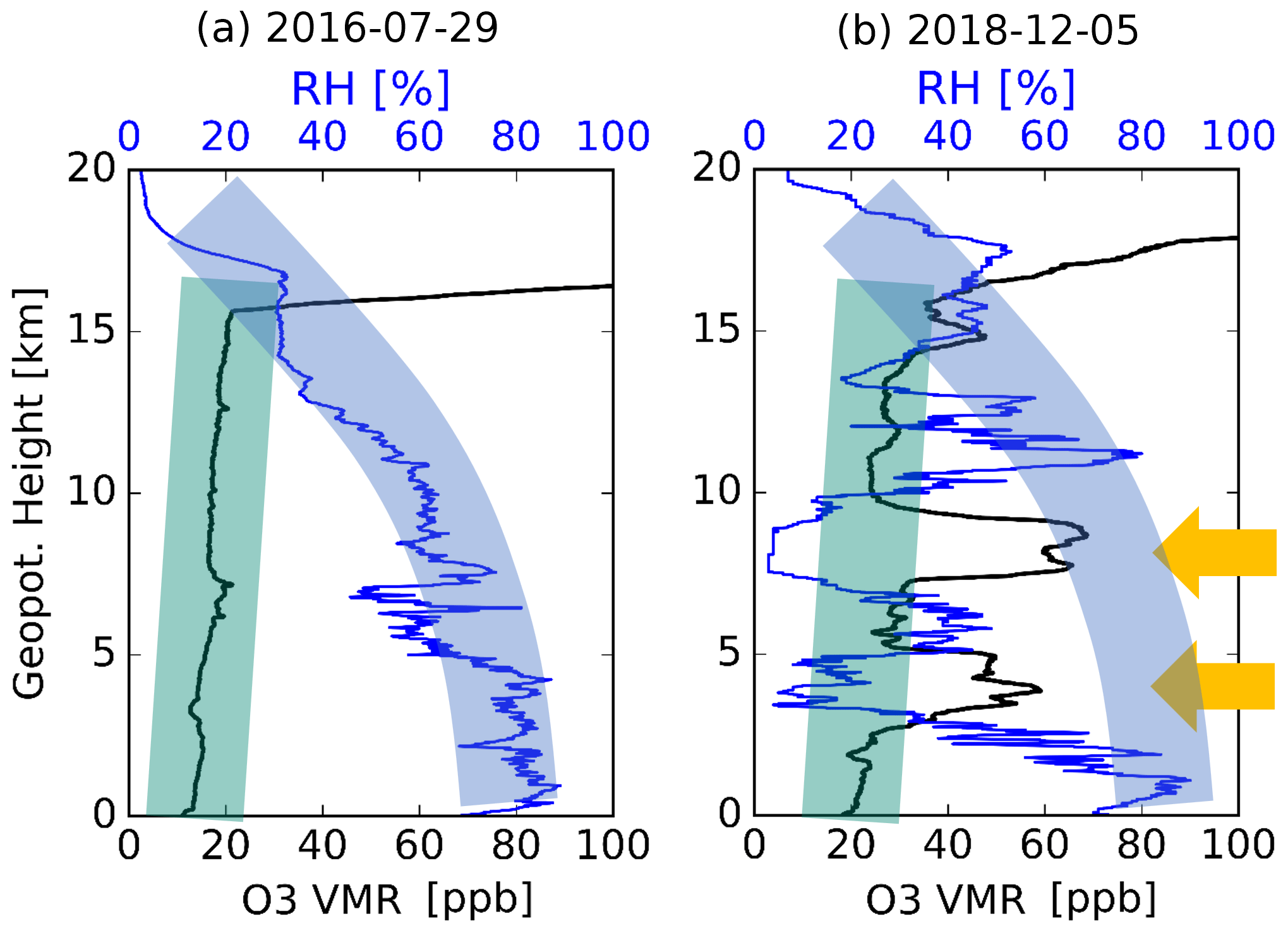
Figure 2 Example tropospheric O₃ VMR (black lines) and RH (blue lines) profiles from the PAO for the background atmosphere (a) and anomalously dry ozone-rich layers (b). The ideal shape for the background atmosphere in (a) is illustrated in green and blue shading; two layers disrupting the respective background are indicated by yellow arrows in (b).

Layered structures of higher O₃ VMR in the mid-troposphere disturbing the uniform low O₃ profile are often observed and a signature of non-local air masses (e.g., Pan et al., 2015; Anderson et al., 2016; Randel et al., 2016). Figure 2b shows an example profile with two distinct layers of enhanced O₃ levels (> 50 ppb) around 4 and 8 km, interrupting otherwise quite constant levels of low O₃ VMR (∼ 25 ppb). Enhanced tropospheric O₃ levels are generated either by photo-chemical processes in high tropospheric NO_x regimes, i.e., in polluted air masses, or by photo-dissociation of O₂ in the stratosphere and subsequent transport to the troposphere. In situ net O₃ production is unlikely at this altitude in the remote TWP, which is far from pollution sources and shows a lack of lightning activity (Christian, 2003; Cecil et al., 2014). Free tropospheric O₃ lifetimes are on the order of weeks and comparable to the dynamical timescales of long-range transport within the tropics and from the subtropics (e.g., Folkins, 2002; Ploeger et al., 2011). Thus, air masses transported either from polluted areas elsewhere or the extratropical stratosphere can retain their high O₃ VMR until arrival in the deep tropics.

To complement O₃ as an indicator of air mass origin, we made use of RH as a measure of vertical displacement of air masses. The benefit of using RH is the readily available data from the combined sonde measurements. The dominant anti-correlation between O₃ and RH in the PAO dataset further suggests closer examination of RH (Figs. 1 and 2). RH allows us to distinguish between different underlying processes affecting either local or non-local air masses (e.g., Hayashi et al., 2008; Schoeberl et al., 2015). Local air masses of low O₃ VMR often show high RH values (O₃−RH+) in accordance with the assumed dominance of convective activity and uplift. The example in Fig. 2a shows that RH values characteristically decrease with altitude but remain greater than 45 % throughout the mid-troposphere (cf. Mapes, 2001). Non-local, ozone-rich air masses often correspond to low RH compared to the air masses above and below the humid tropical column (O₃+RH−). The depressed RH levels can be explained by either stratospheric origin or various dynamical processes during transport, mostly involving a descent of air masses towards Palau that results in adiabatic compression and heating of the air, reducing RH at constant absolute humidity (Cau et al., 2007; Dessler and Minschwaner, 2007; Anderson et al., 2016). The study of RH data thus supports our understanding of processes governing O₃ variability above Palau.

The competing hypotheses for the genesis and origin of O₃+RH− air demand the use of an additional tracer (e.g., Stoller et al., 1999). In this study, we use potential vorticity (PV) as a dynamical tracer to identify a potential stratospheric origin of air masses. We assume a significant in-mixing of extratropical stratospheric air for air masses with an absolute PV greater than 1.5 PVU for at least 1 d during 10 d before arrival in Palau (Waugh and Polvani, 2000; Kunz et al., 2011).

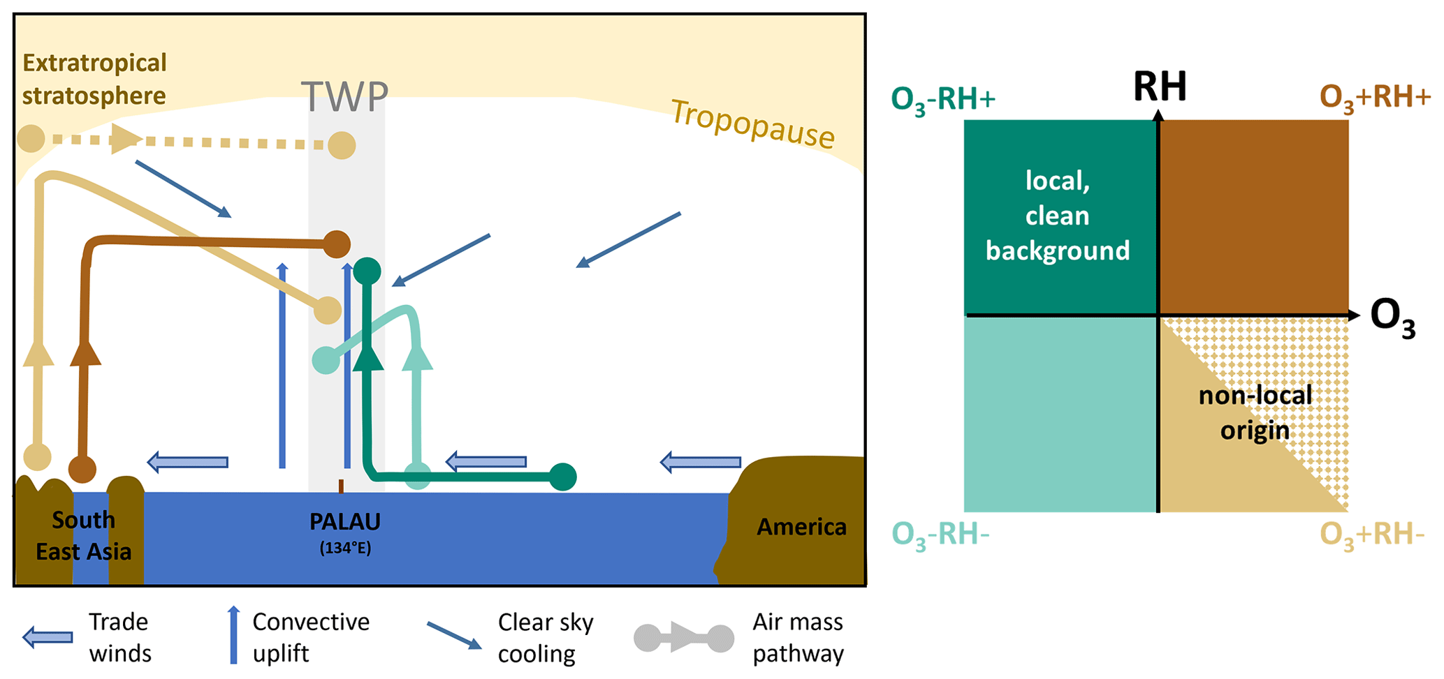
Figure 3 Schematic for transport pathways to Palau and the TWP on the zonal plane. Major dynamical drivers are marked with arrows (blue colors), while transport pathways are color coded according to the air masses' O₃ $/$ RH characteristics shown in the qualitative grid (turquoise colors for O₃−, brown colors for O₃+, hue for RH±). O₃+RH− air (light brown) masses above Palau may have followed two of the five shown pathways, indicated by a solid and dotted line in the schematic (for details, see Sect. 3.1.1).

In conclusion, we propose four qualitative categories of air masses and five different pathways identifiable by our tracers, as illustrated in Fig. 3. Ozone-depleted air masses (O₃−, turquoise colors) are of local or Pacific convective origin, and ozone-rich air masses (O₃+, brown colors) originate from non-local pollution or the stratosphere. High RH results from a dominant convective uplift of air masses (RH+, darker hues), while low RH indicates a stratospheric origin or dehydration of previously lifted air masses during transport due to clear-sky cooling and descent (RH−, lighter hues). O₃+RH− air is characteristic for two different pathways (solid and dotted light brown lines in Fig. 3), thus representing two different types of air masses.

As discussed above, the two important air mass categories are tied to the dominant anti-correlation of O₃ and RH above Palau: O₃−RH+ background air and O₃+RH− air masses occurring mostly in layers interrupting the background. Air masses with positively correlated O₃ and RH are observed less often and are more difficult to assess. O₃+RH+ air masses (dark brown) are potentially caused by non-local pollution convectively lifted in the source region and transported rapidly towards Palau on the same altitude, conserving the high humidity. We further suggest that O₃−RH− air (light turquoise) consists of clean boundary layer air convectively lifted in the Pacific vicinity of Palau, dehydrated due to clear-sky cooling during transport. Other processes, like remoistening or in-mixing of midlatitude air during transit to the TWP could also play a role (Cau et al., 2007; Sherwood et al., 2010; Schoeberl et al., 2015; Tao et al., 2018) and are difficult to assess just using the tracer data.

3.1.2 Previous approaches

To detect and assess anomalous layers from balloon and aircraft profiles, different methods have been applied (Stoller et al., 1999; Thouret et al., 2000; Hayashi et al., 2008; Pan et al., 2015). Stoller et al. (1999) used data from three NASA campaigns (PEM-Tropics, PEM West A and B) to calculate a free tropospheric background mode for various atmospheric constituents (O₃, H₂O, CO, CH₄) and for individual profiles. Using a spike detection approach, they produced extensive statistics for the frequency of anomalous layers in the whole tropical Pacific region for two different seasons. The same methodology was applied to MOZAIC aircraft data by Thouret et al. (2000). Its main disadvantage lies within an arbitrary threshold used to determine the background mode. Despite the statistical uncertainty, Stoller et al. (1999) recognized the importance of anomalous layers in tropical Pacific profiles and emphasized their role in atmospheric chemistry modeling due to their frequent occurrence.

A similar analysis of longer time series from three SHADOZ sites (Southern Hemispheric Additional Ozonesondes Network; Thompson et al., 2003a, b, 2012, 2017) confirms the frequent occurrence of dry enhanced O₃ layers below 12 km (Hayashi et al., 2008). Using a statistical method for the layer detection, the study found respective layers in approximately 50 % of profiles per year and station with differing seasonal variations. The study relies on the separation of a wet and distinct dry season at the respective stations, which is not applicable for the Palau site (see Müller et al., 2024).

Pan et al. (2015) isolated the low O₃ background or “primary mode” by removing all “dry” data with RH less than 45 % for all observations during the CONTRAST campaign (Pan et al., 2017). They thus refrained from resolving the individual vertical structure of layers but proposed the RH threshold as an overall criterion in the free troposphere to separate local and non-local air masses. Pan et al. (2015) emphasized the possible variability of air mass origin within the individual vertical column, which is obscured in seasonal or even annual profile averages, i.e., layered structures in the O₃ profile hidden within the typical so-called “S” shape (cf. Sect. 4.1). Their method, however, seems limited to the specific sites and season of the CONTRAST campaign, as it does not yield a robust output for the Palau data during all seasons (Müller et al., 2024).

3.1.3 Statistical definition of background and anomalies

For a quantitative definition of air masses above Palau, we first determined background profiles in the free troposphere from the PAO O₃ and RH time series. These profiles represent humid, ozone-poor, local air masses that are controlled by convective influence and not by long-range transport. This was performed on a statistical and monthly basis and aimed to identify profile shapes similar to the signature profiles in Fig. 2a. For the monthly O₃ VMR background profiles we chose the 20th quantile (Q20) profiles. Q20 guarantees sufficiently low O₃ values to avoid a “belly” shape in the profiles, typical for tropical average O₃ profiles. For the monthly RH background profiles we chose the 83.3th quantile (Q83) profiles. Q83 is the upper boundary of the central 66.6 % range, guaranteeing high humidity. Figure 4 shows an example of these background profiles for March. The monthly quantile profiles have been vertically smoothed using first a 1 km binning and then exponentially weighted moving averages with altitude (see also Figs. A3 and A4). Figure 4 includes the median and central 66.6 % ranges for both tracers separately and is calculated from 16 individual profiles (see Müller, 2020, for more details).

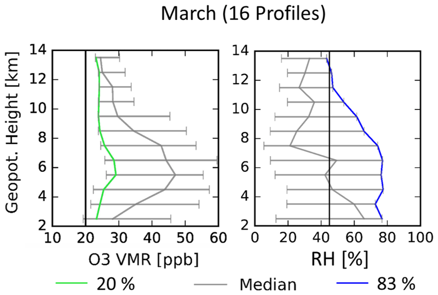
Figure 4 O₃ VMR and RH statistics for the month of March as example for Palau free tropospheric profiles as a function of altitude: the 20th quantile (Q20) for O₃ is shown in green, and the 83.3th quantile (Q83) for RH is shown in blue (both vertically smoothed using exponentially weighted moving averages). The median is marked in grey, and the central 66.6 % range is shown by grey horizontal bars. The number of included individual profiles is shown in brackets, and for orientation 20 ppb O₃ VMR and 45 % RH are marked in black (see also Figs. A3 and A4).

Our method roughly followed the approach of Hayashi et al. (2008). However, Hayashi et al. (2008) defined air masses above the 83.3th quantile as O₃ enhanced layers. With the Q20 limit for O₃ we used a less conservative approach because the Palau background atmosphere is characterized as a uniform, well-mixed low O₃ profile, caused by uplift of ozone-poor boundary layer air in active convection. We chose this particular O₃ quantile to yield the most uniform, “straight-line” profile in the free troposphere for all monthly averages of the given time series. This essentially smoothes out any interrupting layers occurring at varying altitudes in individual profiles. While Hayashi et al. (2008) analyzed RH in ozone-enhanced anomalous layers in contrast to the air masses above and below, we applied the statistical approach to both tracers and chose Q83 for RH to detect typical convection associated with the background. The resemblance of both the particular low O₃ and high RH quantiles with the example of an individual background profile in Fig. 2a is evident. The monthly averaging accounts for the seasonal variability of the background as the uniform O₃ profile shifts towards higher base VMR from summer–fall to winter–spring (cf. Figs. 2 and A3).

In a second step, we determined the anomalies against the monthly background profiles, denoted in the following by ΔO₃ and ΔRH. These are calculated for individual measured O₃ $/$ RH pairs within each sounding and in their respective month–altitude bin. Within the anomaly space, we define a new background air mass category, “ΔO₃∘ΔRH∘”, with close to zero anomalies in both tracers. We further denote eight other quantitative air mass categories with combinations of positive (“+”), negative (“−”) or close to zero (“∘”) anomalies for both ΔO₃ and ΔRH individually (Sect. 4.1.3). In this study, however, we limited further analyses to the two most interesting quantitative air mass categories, ΔO₃∘ΔRH∘ and ΔO₃+ΔRH−, i.e., per definition humid, ozone-poor background air masses and anomalously dry, ozone-rich air masses. In contrast to Hayashi et al. (2008) we did not assess the vertical structure of the anomalous layers in individual profiles. Hence, neither the layer thickness nor the layer position within the profile were considered. Any measured data point of a profile was quantitatively attributed to one of nine air mass categories, which were then analyzed “in bulk”. In our following analysis, we further focused on the altitude region between 5 and 10 km, where the weakest cloud mass divergence occurs, i.e., the weakest convective detrainment (Folkins and Martin, 2005) and the greatest frequency of anomalous layers.

3.2 Trajectory analysis

We deployed the trajectory module of the fully Lagrangian chemistry and transport model ATLAS (Wohltmann and Rex, 2009; Wohltmann et al., 2010) driven by ERA5 data (see Sect. 2). The model uses a hybrid vertical coordinate, which gradually transforms from pressure at the surface to potential temperature in the stratosphere. The corresponding vertical velocities change from vertical winds in pressure coordinates to diabatic heating rates, respectively.

The 10 d backward trajectories with a time step of 10 min were initialized at the location and time of every 10th sonde reading of a profile (approximately every 50 m, i.e., 20 trajectories per kilometer) for all profiles within the trajectory dataset. They are considered as a footprint for transport pathways towards Palau. We assume O₃ to be a passive tracer during transport, i.e., did not implement chemical reactions. This assumption is justified for dry, mid- to upper-tropospheric air because of photo-chemical lifetimes of O₃ on the order of several weeks to months under these conditions. In the wet lower troposphere and marine boundary layer this approach is only valid for a few days because of O₃ lifetimes on the order of days (e.g., Thompson et al., 1997). Convection is not treated explicitly in the model setup, but partly reflected in the reanalysis data. Anderson et al. (2016) found air parcel ages of around 10 d in the TWP in winter 2014, when stopping their trajectories at the point of last precipitating convection based on satellite observations of cloud top height and precipitation. We therefore assume no “reset” of the composition of our air mass within 5 d and stop our trajectories 5 d before arrival to identify the origin.

4 Results

We first present the variability of the PAO tropospheric O₃ time series to assess air mass seasonality and the application of our method to determine different groups of air masses. Then, our results from the trajectory analysis are shown, first by investigating general seasonal tracer variability and second by combining these results with our method to identify different air masses (Fig. 3). A physical interpretation of the results follows in the discussion (Sect. 5).

4.1 Air mass variability

4.1.1 Annual O₃ variability

Figure 5 shows time–height cross-sections of the annual variability of tropospheric O₃. Figure 5a shows monthly means, Fig. 5b shows anomalies from the annual mean profile and Fig. 5c shows the annual mean profile of the overall time series (solid black line), excluding El Niño 2016. Panel (c) also shows the standard deviation (SD) and the relative standard deviation (RSD) of the overall annual mean profile (dashed and dotted lines, respectively), as well as the annual mean profiles of individual years (colored lines). As the fraction of the SD relative to the annual mean, the RSD can be considered as a measure of variability with altitude (cf. Ogino et al., 2013). The annual mean tropospheric O₃ VMR profile (Fig. 5c) has an S shape typical for tropical sounding stations (e.g., Folkins, 2002; Thompson et al., 2003a, b; Pan et al., 2015). O₃ VMR are lowest in the boundary layer (< 20 ppb) and also low between 10 and 12 km (< 30 ppb). They increase in the mid-troposphere to about 35 ppb and again above 12 km towards their stratospheric maximum, which is an order of magnitude higher. The interannual variability of the annual mean O₃ profile is low for all years, with the exception of 2016.

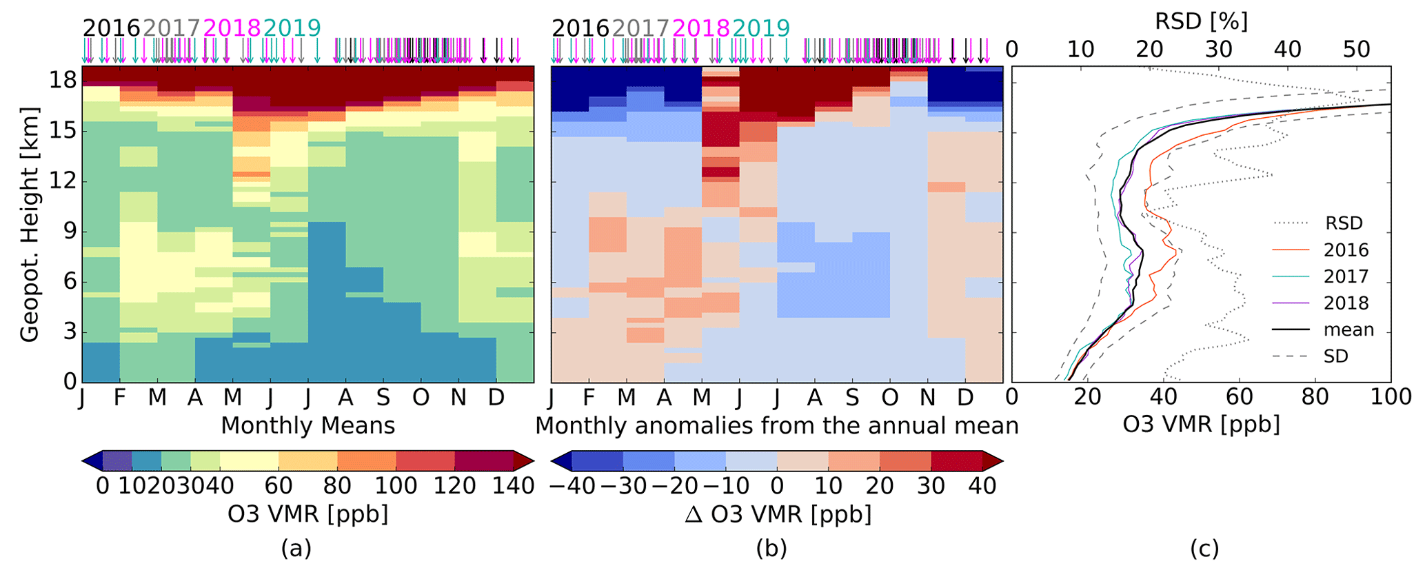
Figure 5 Monthly means (a), anomalies from the annual mean (b) and the annual mean profiles (c) for individual years (thin colored lines) and for the whole time series excluding El Niño 2016 (thick black line) with standard deviation for the whole time series (dashed grey lines) and relative standard deviation (RSD) (dotted grey line). Individual soundings are marked as arrows above with different colors for different years. Nonlinear scaling is used in (a) to match the different orders of magnitude in the lower and upper troposphere (cf. Müller et al., 2024, Fig. 6).

The monthly O₃ VMR (Fig. 5a and b) reveal two dominant signals: an annual cycle in the 5–10 km altitude range with the maximum from February until April (30–60 ppb) that is 2–3 times greater than the minimum from July until October (10–30 ppb) and a reverse, strong cycle in the TTL with maximum anomalies (> 40 ppb) from June until September. The peak in RSD of 50 % at about 17 km reflects the strong TTL cycle. The enhanced variability in mid-tropospheric O₃ (RSD ∼ 30 %) corresponds with the cycle revealed by the monthly means. Annual variations in O₃ observations are smallest between 10–12 km and especially in the boundary layer (RSD ∼ 20 %), and these are thus coincidental with the O₃ minima of the annual profile. The regionally typical ozone-poor background is clearly subject to seasonal variations.

4.1.2 Seasonal O₃ profiles

A more detailed analysis of the seasonal O₃ variability helps to identify recurring seasonal characteristics and differences in controlling processes like synoptic or meteorological conditions. Therefore, we divided our time series into four seasons, shifted by 1 month compared to the temperate climate seasons: November–December–January (NDJ), February–March–April (FMA), May–June–July (MJJ) and August–September–October (ASO). These Palau seasons reflect different influences dependent on the time of the year and were chosen empirically by sorting monthly O₃ profiles (Müller et al., 2024, Fig. A1) by similar shape, considering the full free troposphere. The resulting four most different types of profile shapes are shown in Fig. 6. The Palau seasons turned out to be centered around the equinoxes, which is reasonable for a tropical station.

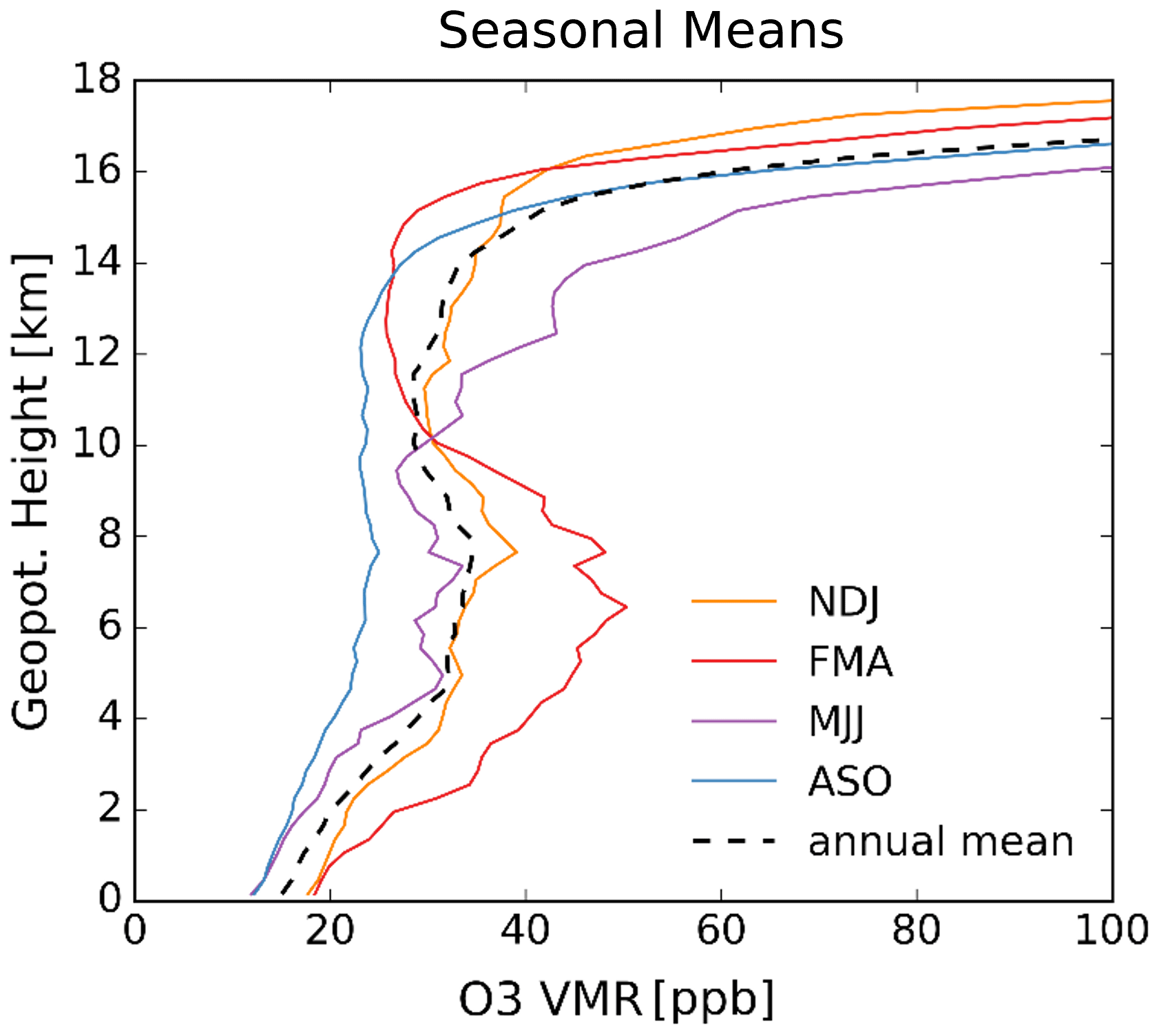
Figure 6 Seasonal mean O₃ VMR profiles (solid colored lines) in comparison to the annual mean (dashed black line), all excluding El Niño 2016, for Palau seasons November–December–January (NDJ), February–March–April (FMA), May–June–July (MJJ) and August–September–October (ASO).

In the 5–10 km altitude range FMA and ASO show the largest differences and represent the extremes of the mid-tropospheric cycle. The S shape of the annual mean profile prevails in the winter seasons, i.e., in NDJ and most pronounced in FMA. The interannual variability is particularly high during FMA from 5 to 10 km with generally enhanced O₃ VMR between 40 and 50 ppb (Fig. A1). The ASO profile is closest to the uniform background profile (20–25 ppb O₃ VMR) with little interannual variability, while having the highest sampling rate (59 profiles). We thus refer to ASO as the background season. In the TTL, both extreme seasons, ASO and FMA, show a pronounced O₃ minimum, except during the 2016 El Niño FMA season (Fig. A1). The steep onset of higher levels of (stratospheric) O₃ VMR in ASO occurs at lower altitudes compared to the NDJ and FMA seasons.

MJJ and NDJ can be considered as intermediate seasons with respect to the mid-tropospheric cycle; i.e., O₃ values here are in between the minimum and maximum. The NDJ profile resembles the annual mean profile up to about 14 km, while the MJJ profile diverges from the annual mean above 10 km towards higher values. The resulting tilted line shape during MJJ, compared to the straight line profile during ASO, implies a more gradual increase of O₃ in the upper troposphere–lower stratosphere (UTLS) (cf. Müller et al., 2024) and a lack of a pronounced O₃ minimum in the UT. In MJJ, the tropopause is at its lowest altitude of the year, which is also the case for the occurrence of high levels of stratospheric O₃ VMR.

4.1.3 O₃ and RH: background and anomalies

The application of our method to separate air masses on the full PAO time series for the free troposphere (3–14 km) yields the distribution of anomalies from the background profiles, ΔRH and ΔO₃, given in Fig. 7 (see also Sect. 3.1.3). The 2D histogram in Fig. 7a shows ΔO₃ versus ΔRH from all months and altitudes as percentages of the total count of all measured free-tropospheric O₃ $/$ RH data pairs in greyscale. Data along the zero lines within this anomaly space indicate zero anomalies and thus an attribution to the respective background profiles, Q20 of monthly O₃ VMR and Q83 of monthly RH values. The marginal 1D histograms show the distributions of both tracers individually normalized to unity.

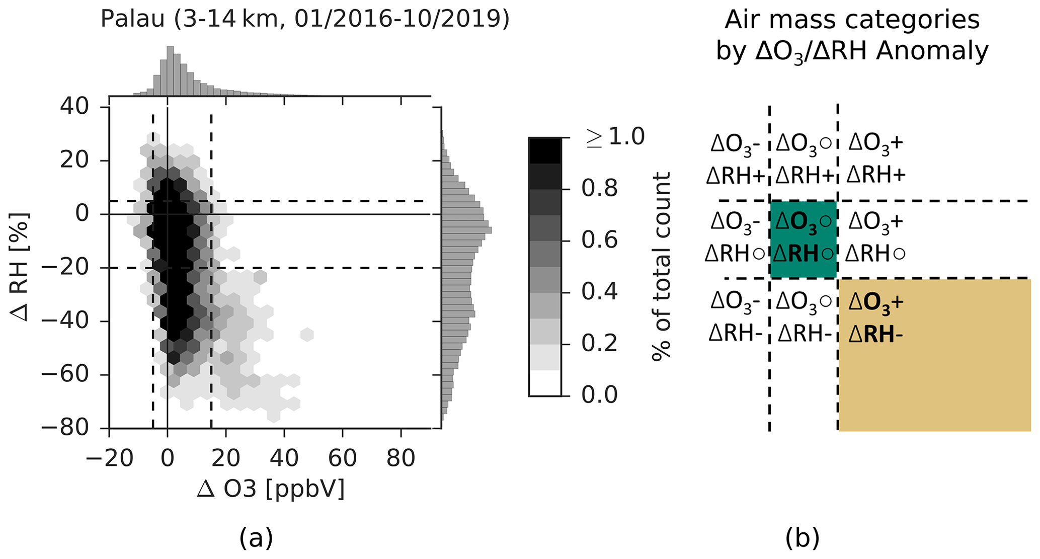
Figure 7 (a) Free-tropospheric (3–14 km) relation between tracer anomalies ΔO₃ VMR and ΔRH from monthly background profiles defined in Sect. 3.1. Color shading indicates percentages of total count of measured O₃ $/$ RH data pairs per grid point. Marginal plots for individual tracer anomaly distributions are normalized to unity. Dashed lines refer to quantitative air mass categories in the 3 × 3 quantitative grid as illustrated in (b), with boundary values for the central grid box (ΔO₃∘ΔRH∘) of −5/+15 ppb for ΔO₃ VMR and −20 %/+5 % for ΔRH. Two target categories of the analysis are highlighted in color in (b) (cf. Fig. 3).

Both ΔRH and ΔO₃ show heavily skewed distributions, with a long tail in the ΔO₃ distribution towards less frequent high O₃ occurrences and even a bimodal distribution for ΔRH with a secondary maximum in the tail towards dry air masses. These distributions motivate the separation of air masses into three domains for both parameters, with one corresponding to the low tail, one to the bulk of the observations and one to the high tail. Overall this leads to nine quantitative air mass categories in a 3 × 3 grid that is referred to as the quantitative grid (Fig. 7b). The boundaries were chosen empirically with respect to the shape of the distributions with a range of −5/+15 ppb ΔO₃VMR and −20 %/+5 % for ΔRH for the central group.

In particular, the correlated occurrence of air masses with high O₃ and low RH (ΔO₃+ΔRH−) stands out as a low but separate population in Fig. 7a (lower-right quadrant), while the central group (ΔO₃∘ΔRH∘) represents the most frequent conditions and is referred to as background category (not to be confused with the background profile) since anomalies from the background profiles are smallest. In this study, we focus on the distinct population of ΔO₃+ΔRH− air masses in contrast to this background category. ΔO₃∘ΔRH∘ air masses are characterized by significantly higher RH and lower O₃ and are therefore also referred to simply as the humid, ozone-poor background.

The anomalies are mostly clustered within 20 ppb along the ΔO₃ zero line indicating an overall dominance of ozone-poor air masses. Apart from the tail towards less frequent higher ΔO₃, the narrow distribution is nearly Gaussian and centered around 0 ppb ΔO₃ VMR with a tendency towards positive values. The majority of ΔRH values appear between −60 % and 20 %. The bimodality of the ΔRH distribution is persistent in all seasons with the exception of MJJ (Fig. A5). The primary, dominant mode is centered slightly off the ΔRH zero line towards negative values, i.e., the majority of measured RH values match the Q83 or slightly lower values of the respective month–altitude bin. The secondary mode occurs for ΔRH values 40 % lower than their background profile estimates.

Figure 8 Seasonal free-tropospheric (3–14 km) relation between tracer anomalies ΔO₃ VMR and ΔRH. The total number of data points is given in brackets, colors are according to Fig. 6, and more details are given in Figs. 7 and 6.

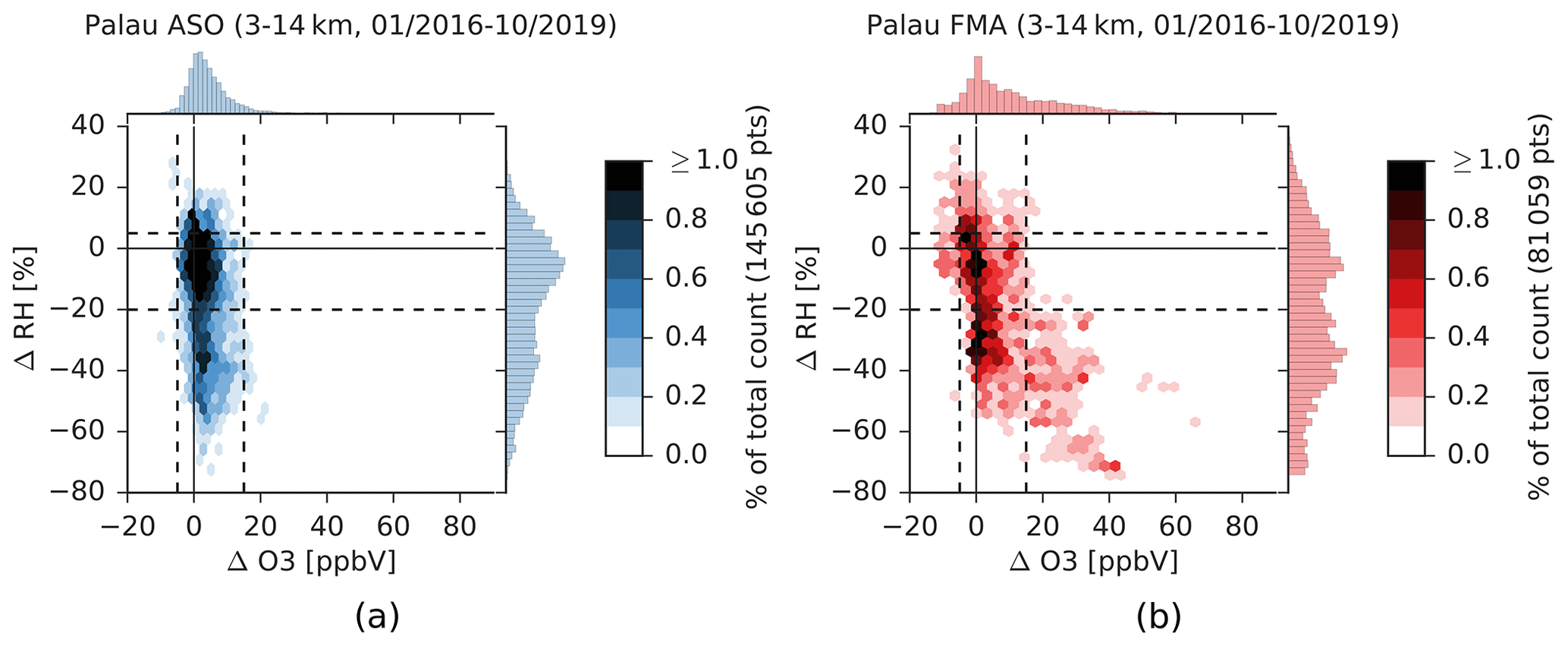
Figure 8 shows the ΔO₃ $/$ ΔRH distribution for the seasons FMA and ASO. As expected from the previous analysis, ΔO₃+ΔRH− are almost absent in ASO (Fig. 8a), emphasizing that the season represents an overall ozone-poor, mostly humid background in the free troposphere. In contrast to the seasonal mean FMA O₃ profile with elevated O₃ levels in the mid-troposphere (Fig. 6), the FMA anomalies distribution (Fig. 8b) reveals a dominance of background category air masses over ΔO₃+ΔRH− air masses within the free troposphere. A statistical view on the seasonal occurrence of different air masses in the mid-troposphere emphasizes the year-round dominance of ΔO₃∘ΔRH∘ air, which were observed in more than 70 % of profiles within each season (Fig. A6).

4.2 Air mass transport and processes

4.2.1 Trajectory origin by season

In the following, we focus on the 5–10 km altitude range with the most frequent occurrence of ΔO₃+ΔRH− air masses and the largest seasonal differences in O₃ VMR (cf. Fig. 6 and Sect. 3.1.3). A footprint of air mass transport to Palau is analyzed using 10 d backward trajectories for the study period (2016–2019) sorted by season arriving in Palau in the 5–10 km altitude range (Fig. 9). For better visualization, a representative subset was chosen, displaying only every 20th trajectory of a profile (roughly one trajectory per kilometer). Colored line segments show three different time periods backwards, 3, 5 and 10 d, thus indicating the velocity of air mass transport.

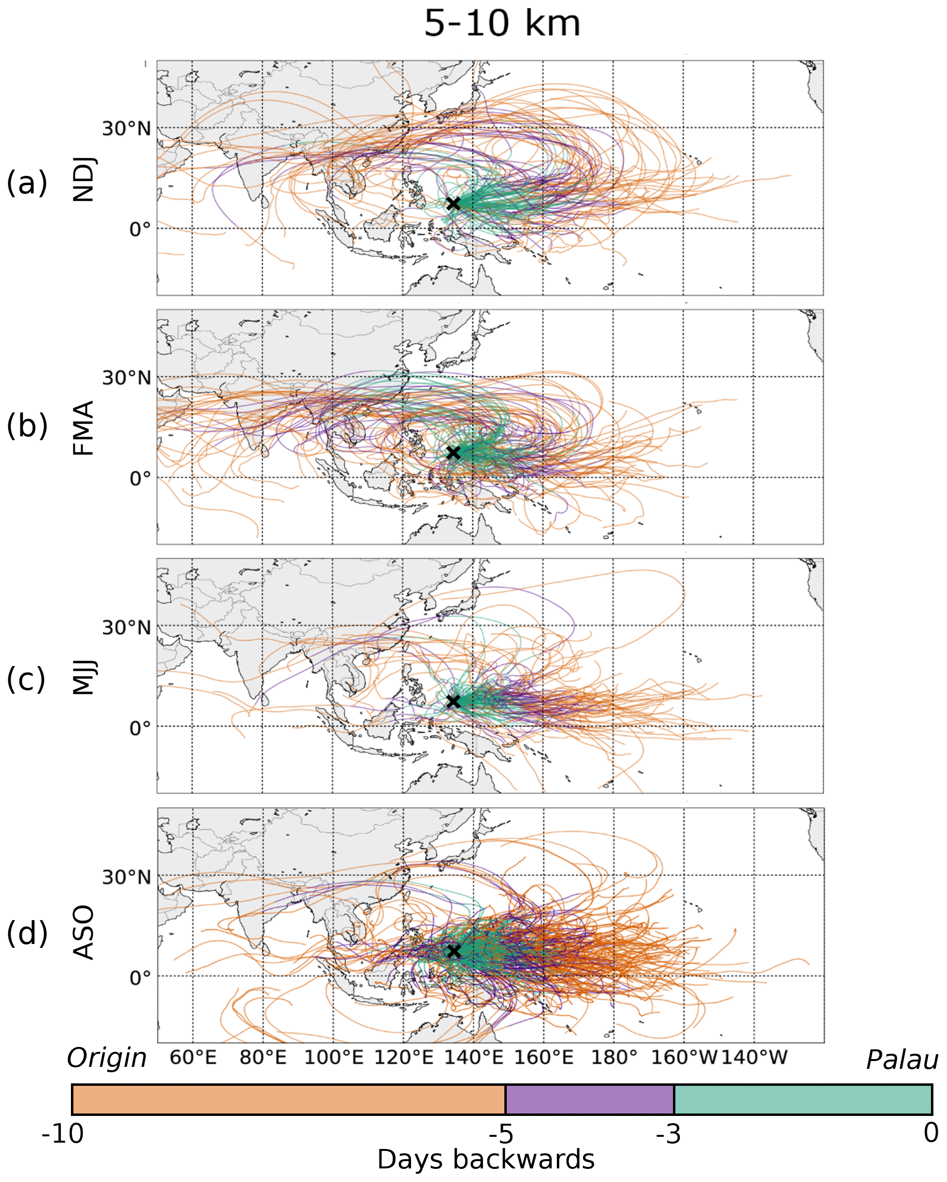
Figure 9 Geographical footprint of air masses. The 10 d backward trajectories from ATLAS arriving at Palau in the 5–10 km altitude range by season (2016–2019). Colored segments represent time periods of maximal 3 (green), 5 (purple) and 10 d (orange) backwards, respectively. The x marks the location of Palau. Only a subset (every 20th data point of a profile, roughly one per kilometer) of the trajectory dataset is shown; see Fig. 6 for seasons.

Most air masses reach Palau from the east but have traveled two different paths on different timescales. The seasonal distinction of trajectories roughly separates an eastern Pacific pathway, dominating in MJJ and ASO, from an anticyclonic route in NDJ and FMA, connecting Palau with Southeast Asia and some remote areas as far as the African continent. The anticyclonic route can be associated with long-range transport on shorter timescales compared to the Pacific route. As these transport patterns are most pronounced in FMA and ASO, respectively, which also exhibit the greatest tracer differences in the mid-troposphere (cf. Fig. 6), we focus on these two Palau seasons in the following.

The geospatial extent of the footprints differs significantly for season FMA and ASO. While all trajectories stay mostly within the tropical zone between 0 and 30° N, trajectories during FMA have a wider longitudinal extent than during ASO. Most ASO air masses never left the Pacific Ocean area within 10 d before arrival in Palau and have traveled shorter distances. Only a few trajectories on a Southern Hemispheric cyclonic route show the influence of the western Pacific monsoon, which is active from July to October but governs air mass transport mostly below 5 km altitude (Müller et al., 2024).

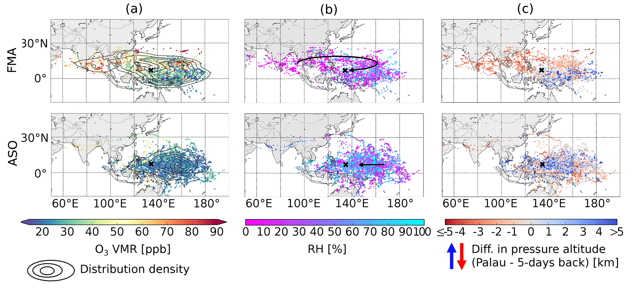
Figure 10 Origin of air masses by season. Location of air masses 5 d before their measurement in Palau in the 5–10 km altitude range inferred from trajectories for Palau seasons FMA (upper row) and ASO (lower row), which have been color coded by O₃ VMR (a), RH (b) and by difference in pressure altitude between the measurement and 5 d before the measurement (c). Black contours in (a) show distribution density, and schematic arrows in (b) indicate the pathway as shown by the footprint in Fig. 9; see Fig. 6 for seasons.

Figure 10 shows the location of air masses 5 d before their measurement in Palau inferred from trajectories for the seasons FMA (top) and ASO (bottom) as an indication of the origin of the air masses. The geospatial probability density function of data points is highlighted as black contour lines in Fig. 10a. Here, the colors indicate O₃ VMR as observed upon arrival in Palau. Figure 10b and c show the same locations as Fig. 10a but are color coded by RH (Fig. 10b) or difference in pressure altitude (Fig. 10c). Red colors in panel (c) indicate descent, while blue colors indicate ascent towards Palau.

The dominant source region of free-tropospheric Palauan air masses, indicated by the center of the density distribution in Fig. 10 a, is located east of Palau during both seasons and corresponds to low O₃ VMR (≤ 30 ppb). During FMA, this eastern center of the distribution is actually split in two parts along a latitudinal axis. The dominant part is located further south on the Equator, exhibiting low O₃ VMR. The northern part of the eastern center is of higher O₃ VMR. A separate cluster of trajectory points showing enhanced O₃ VMR (≥ 60 ppb) exists northwest of Palau during FMA, roughly extending from India to Taiwan. As revealed by the full 10 d trajectories in Fig. 9b, all air masses of higher O₃ VMR during FMA can be related to the anticyclonic route, though some took longer than 5 d to travel from Southeast Asia to Palau. During ASO the overall unimodal distribution is centered on Palau's latitude, 20° to the east, and observations of enhanced O₃ VMR originate outside the main cluster. For both seasons, air masses with O₃ VMR greater than 60 ppb rarely originate south of Palau.

The distinction between the two pathways is also reflected in RH (Fig. 10b) and even more clearly in the vertical displacement of air masses from origin to destination (Fig. 10c). In FMA, Fig. 10c shows descended air masses originating north and ascended air south of Palau. Here, the descent of air masses corresponds with greater O₃ VMR and lower RH, although the pairwise correlation, R, of these two parameters with the pressure height difference is not strong ($R=-\mathrm{0.53}$ for O₃VMR and R=0.44 for RH, for the latter cf. Fig. A7). We can, however, associate these dry, descending air masses with the anticyclonic route shown in the 10 d backward trajectory footprint.

For ASO air masses, the picture is not as clear, but ascent and humid air masses with low O₃ VMR are slightly dominating (Figs. 10c and A7b) and have likely followed the Pacific pathway. The pairwise correlation for pressure–height difference and O₃ VMR or RH, respectively, is even lower than during FMA ($R=-\mathrm{0.36}$ for O₃, R=0.35 for RH). However, there are clearly two main groups of air masses, one with RH below 40 %, descended mostly by only 1 km, and one group with RH centered around 70 %, ascended mostly by 1 km or more.

The investigation of the history of PV for Palauan air masses revealed no stratospheric pathway. Below 1 % of all 13 627 trajectories stayed above 1.5 PVU for more than a day during 10 d transit to Palau. Within 5 d before arrival only a few trajectories crossed the 1.5 PVU threshold.

4.2.2 Trajectory origin by air mass

While we have looked at the origin of the trajectories as a function of season in the previous section, we now turn to the origin as a function of air mass. The classification of trajectories by quantitative air mass category as defined in Sect. 3.1 yields the distribution of source regions as shown in Fig. 11. Background ΔO₃∘ΔRH∘ air masses originate within a compact region in the Pacific, mostly east of Palau and stretching as far as 180° E. The origin pattern for ΔO₃+ΔRH− air masses clearly shows transport from the Southeast Asian region and along the anticyclonic path to Palau. In comparison to the seasonal analysis, the classification of trajectories by air masses shows a clear distinction for the history of vertical displacement of the air masses. On their way towards Palau most ΔO₃∘ΔRH∘ air masses have been ascending, while ΔO₃+ΔRH− air has descended.

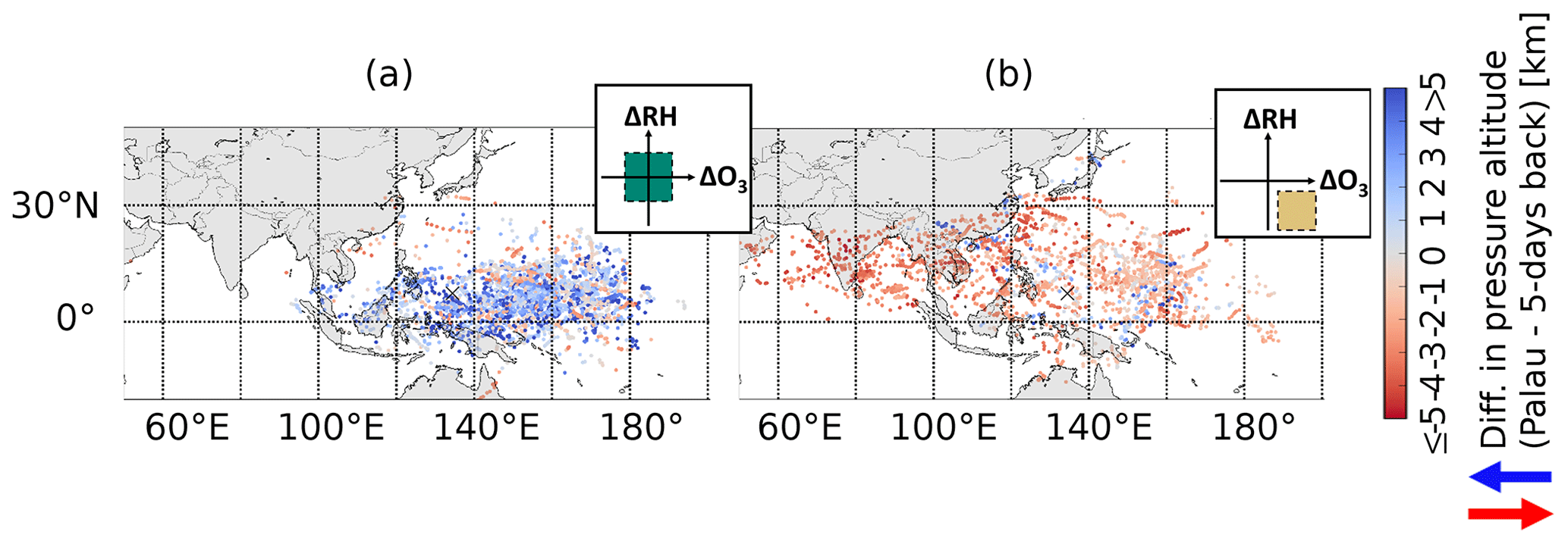
Figure 11 Origin of air masses by air mass anomalies. Location of air masses 5 d before their measurement in Palau in the 5–10 km altitude range inferred from trajectories for ΔO₃∘ΔRH∘ (a) and ΔO₃+ΔRH− (b) air masses, as indicated by the pictograms. These are color coded by the difference in pressure altitude between the measurement and 5 d before the measurement; see also Figs. 7 and 10.

A seasonal analysis of the trajectories sorted by air mass anomalies reveals some differences in the source regions of ΔO₃+ΔRH− air masses (Fig. A8). The origin hotspots around India and the Southeast Asian peninsula are almost exclusively observed during FMA. The southern Philippines and the area slightly northeast of Palau are equally dominant source regions in this season. In ASO, ΔO₃+ΔRH− air masses are less frequently observed, and their origins are clustered around three main areas: (1) northeast of Palau in the western Pacific, (2) between Borneo and the southern Philippines, and (3) in the New Guinea region, extending towards northern Australia.

5 Discussion

The central goal of our study was to identify the air mass origin of TWP air and its seasonality by means of the observed O₃ $/$ RH relation above the PAO. We proposed a qualitative transport scheme for different types of air masses (O₃±RH±, Fig. 3) that distinguishes between local and non-local processes. Lagrangian backward trajectories support this hypothesis. Trajectories with different air mass characteristics, defined by their O₃ and RH anomalies from statistically defined background profiles, show different geographical origins and transit properties. The PAO 4-year time series reveals the seasonality of air mass types and thus origin. Our analysis thereby confirms the usefulness of O₃ and RH as combined tracers for air mass origin in the TWP.

5.1 Seasonality and air mass definition

The PAO time series provides unprecedented insight into the seasonality of tropospheric air composition in the TWP (Müller, 2020; Müller et al., 2024). An important observation from the PAO dataset is the dominant anti-correlation between O₃ and RH (Fig. 1). The annual cycles of O₃ in the mid and upper troposphere were expected from satellite observations and previous studies, especially the zonal wave one pattern in the TTL (e.g., Thompson et al., 2003b; Randel et al., 2007) but had not been monitored continuously with in situ measurements before. The high temporal and vertical resolution of the ozonesonde dataset revealed day-to-day variations but also the prevalence of significant seasonal signals modulating these. The increased sampling frequency during the extremes of the mid-tropospheric cycle especially shows the robustness of this signal for Palau and the dominance of the local low O₃ mode during late summer (Fig. 6). Currently, the shortness of the time series and statistical bias due to the differences in monthly sampling frequencies have to be taken into account. A future analysis of the growing time series will be better able to assess the influence of interannual variability. The ENSO cycle will likely play the most important role in this.

The mid-tropospheric O₃ cycle is in accordance with the annual movement of the Intertropical Convergence Zone (ITCZ). The occurrence frequency of either a clean convective (local) state or a non-local state with long-range transport to the TWP is regulated by the two major barriers ITCZ and Southern Pacific Convergence Zone (SPCZ). Müller et al. (2024) showed the correspondence of the ITCZ's position north of Palau with the minimum in O₃ measurements (see Fig. 5). This relates to previous studies on air mass transport to the region: during the PEM-Tropics West B campaign, Browell et al. (2001) found that layers of high O₃ VMR advected to the TWP from remote polluted areas are mostly confined north of the ITCZ. Very low O₃ values were only present in the “equatorial wedge” between ITCZ and SPCZ and associated with enhanced vertical mixing in convection in the absence of gross ground pollution. Palau is enclosed between these bands during ASO (Sun et al., 2023); therefore, it is the best season to observe the clean air background. During FMA, when the ITCZ is located furthest south, transport from higher northern latitudes is possible. MJJ and NDJ can be considered as intermediate seasons with respect to both the mid-tropospheric cycle and the similar location of the ITCZ during its annual crossing. This feature explains why studies related to the CONTRAST campaign that took place in January–February 2014 did not see low O₃ extremes (Pan et al., 2015; Newton et al., 2016; Nicely et al., 2016; Tao et al., 2018), and why background conditions of the region need to be assessed by long-term measurements. Its unique location and year-round operation makes the PAO an excellent background site to study the influence of dynamics (cf. Thompson et al., 2021; Sun et al., 2023).

The strong TTL cycle as a zonal phenomenon can be mostly explained by the interplay between the Brewer–Dobson and Hadley circulations (cf. Müller et al., 2024). Mass fluxes for both circulation regimes become comparable at around 16 km altitude (e.g., Folkins, 2002; Pan et al., 2014). The minimum in the vertical O₃ profile in the UT (the so-called chemopause) can be attributed to deep convective outflow. Recognized as a characteristic feature of tropical profiles, low UT O₃ is often used as an indicator for deep convective detrainment (e.g., Kley et al., 1996; Folkins, 2002; Solomon et al., 2005; Gettelman et al., 2009; Paulik and Birner, 2012). Satellite observations confirm year-round convective activity in Palau, with some variability due to the traverse of the ITCZ twice a year (Gettelman and Forster, 2002; Müller et al., 2024). Müller et al. (2024) associate the occurrence of the strongest winds below 15 km when the ITCZ is furthest south or north of Palau with the poleward branch of the Hadley circulation. The low variability in UT O₃ (Fig. 5c) can hence be explained by the persistence of deep convection and the level of convective outflow in association with the Hadley and Walker circulations (e.g., Folkins, 2002; Solomon et al., 2005; Takashima et al., 2008). The months of May and June stand out in this context with higher O₃ levels between 12 and 15 km thus lacking a chemopause (Fig. 5). The dry environment at this altitude increases O₃ lifetimes and makes in situ O₃ destruction unlikely, although it is discussed as a consequence of convectively injected water vapor (Schoeberl et al., 2015; Anderson et al., 2016). The PAO dataset is predestined for future studies on the seasonality of deep convective outflow and stratosphere–troposphere exchange (STE) processes in the TTL in this region of major entry into the stratosphere in boreal winter.

The specific classification of seasons used in this study corresponds to distinct dynamical conditions. In particular, the Palau seasons can be related to the movement of the ITCZ, the main driver of dynamical variability. Our interpretation of the profile shapes is supported by the separation of trajectory footprints in Fig. 9, i.e., different dominating pathways for the different seasons, and a comparison with an analysis of SHADOZ station profiles from Java and American Samoa by Stauffer et al. (2018). They used a sophisticated clustering technique to characterize ozonesonde profile variability related to different controlling processes. Out of four cluster profiles, the low O₃ cluster associated with convective lifting of low O₃ VMR compares well with the Palau ASO profile. The cluster with highest average O₃ VMR exhibits a similar “tilted line” shape like Palau MJJ with a lower tropopause and weak gradient, explained by Stauffer et al. (2018) with STE. This corresponds well with the minimum annual tropopause height and a shift in wind regimes due to the crossing of the ITCZ around June (Müller et al., 2024). The horizontal wind is weakest throughout the entire tropospheric column in May, as the subtropical ridge shifts south with increasing altitude, which could favor quasi-horizontal transport of extratropical stratospheric air into the TTL. July can be seen as a transition month, as the tropopause is comparable with May and June, but mid-tropospheric O₃ VMR are as low as observed in August and September (cf. Fig. A1 in Müller et al., 2024). In July, the western Pacific monsoon already reaches Palau at lower altitudes in the form of equatorial westerlies, but the tropopause is still low. While the construction of 3-month seasons remains arbitrary in any case, it could be reconsidered especially for the summer months (MJJ, ASO) to further differentiate between these processes.

Our new definition of humid, ozone-poor background and anomalously dry ozone-rich air masses in relation to statistically defined background profiles allows a separation of air mass origin based on backward trajectories. Looking at anomalies, ΔO₃ and ΔRH, our method provides an improved criterion compared to using fixed thresholds based on absolute tracer values, as have been used in previous studies (e.g., Anderson et al., 2016; Nicely et al., 2016; Randel et al., 2016; Tao et al., 2018), who all defined O₃+RH− air masses with RH < 20 % and O₃ VMR > 40 ppb. Our approach using quantiles based on a 4-year time series focuses on a physically motivated background definition. A comparison between air mass categories based on absolute thresholds and our quantitative air mass categories for the PAO dataset shows an improved separation of processes in the trajectory analysis, namely between ascent and descent of air masses (not shown here). The main advantage of our method compared to algorithms of layer detection in individual profiles (e.g., Stoller et al., 1999) lies within its simplicity and the consideration of the identified bimodality in the RH anomalies. In principle, it is also applicable for sounding data time series from other tropical stations. However, it may not yield the best results as atmospheric processes and mechanisms determining air composition might be specific to this geographic region.

The bimodality in RH anomalies is a striking result of our study. It further justifies our separation between ΔRH∘ and ΔRH− air masses in the quantitative grid classification (dashed lines in Figs. 7 and 8), although the exact definition of the grid boundaries could be revisited. Global probability distribution functions of RH from observations have already been shown as bimodal for different tropospheric altitudes in tropical regions, in particular within the ascending branch of the Hadley circulation (e.g., Zhang et al., 2003; Ruzmaikin et al., 2014). Our results fit into the findings of these studies. Other studies, e.g., by Sherwood et al. (2006, 2010), earlier disputed the original claim of a common bimodality in RH distributions by Zhang et al. (2003). The PAO dataset now adds to this discussion. However, a comparison of the different methods arriving at RH distributions would be necessary to draw further conclusions.

A classification of free-tropospheric air mass anomalies by seasons in Fig. 8 shows the absence of ΔO₃+ΔRH− air in ASO and MJJ, as already inferred from the seasonal mean profiles (Fig. 6), compared to their prominent appearance in NDJ and FMA (see marginal 1D histograms for ΔRH in Figs. A5 and 8). During the NDJ and MJJ, both maxima in ΔRH are of similar amplitude, which emphasizes the importance of dry air masses intruding into the otherwise humid troposphere (cf. Stoller et al., 1999). While the relevance of ΔO₃+ΔRH− filaments is undisputed, other categories of air mass anomalies are encountered less often and are thus more difficult to relate to underlying atmospheric processes (cf. Sects. 1 and 3.1.1).

The selection of Q83 for RH could be revisited for the analysis of a larger time series, also in context of the ΔRH bimodality, as the maximum peak of the ΔRH distribution is mostly just below zero, i.e., background values (Figs. 7, 8 and A5). This is also reflected in the dominant occurrence of both ΔO₃∘ΔRH∘ and ΔO₃∘ΔRH− found for the 5–10 km subset of the Palau data (Fig. A6). An adjustment of the RH quantile for the background profile and a corresponding shift onto the center of the ΔO₃∘ΔRH∘ group could still improve the air mass selection. The monthly O₃ profiles are not uniform throughout the column, which is proposed as the ideal, purely convective profile (cf. Figs. 2, A3, A4). During the months of increased occurrence of dry ozone-rich layers, i.e., FMA and NDJ, the Q20 profile still incorporates the S shape, presumably caused by these layers. This effect could possibly be reduced by changing the temporal resolution from monthly to seasonal statistics, which has not been assessed yet. A growing time series will help to validate our approach as it reduces possible biases caused by different sampling frequencies per season.

5.2 Air mass transport and processes

The trajectories reflect the dominating general circulation patterns, namely the Hadley and Walker circulations and the trade winds, with most air masses eventually reaching Palau from the east (Fig. 9). The influence of the western Pacific monsoon, active from July until October, becomes most apparent below 5 km altitude (see Müller et al., 2024). We identified two dominating routes for air mass transport to Palau, the local, Pacific route and the anticyclonic route from Asia. On the anticyclonic route, air masses can travel from the ascending branch of the Hadley circulation towards the descending branch along the subtropical ridge (Anderson et al., 2016). Once air parcels reach the western to central Pacific during winter they are either diverted eastwards by the subtropical high anticyclone or are picked up by the general trade wind circulation, subsequently reaching Palau from the East. In contrast, with a subtropical ridge further north during summer, transport is governed only by the trade winds and monsoon circulation, bringing air masses from the convectively active Pacific region to Palau.

The anticyclonic flow pattern resembles the planetary wave response to tropical diabatic heating as shown for the National Centers for Environmental Prediction (NCEP) reanalysis data by Dima et al. (2005). Following the theoretical concepts of Matsuno (1966), Gill (1980) and Van Tuyl (1986), Dima et al. (2005) identified a pair of upper-tropospheric anticyclonic Rossby gyres located at a maximum of latent heating and directly west of it, i.e., over the western Pacific and Indian oceans. An analysis of the equatorially symmetric component of the circulation pattern reveals the year-round presence of the Rossby wave couplet at 150 hPa, located at the same longitude in the Northern Hemisphere and Southern Hemisphere, with a seasonal shift in longitude for the centers of the anticyclones from approx. 160° E in January–February to approx. 80° E in July–August. At Palau, the anticyclonic flow pattern is indeed dominating for back trajectories above 14 km altitude (not shown here). The equatorially symmetric nature of the Rossby wave couplet is potentially captured by some Palau back trajectories between 5 and 10 km during ASO reaching Palau from the Southern Hemisphere (Fig. 9d). The lack of the anticyclonic route for mid-tropospheric Palau back trajectories for MJJ and ASO and the dominance of the eastern pathway seems to be supported by the seasonal shift in longitude of the centers of the Rossby gyres in the summer months and subsequent stronger easterly flow near the Equator over the western Pacific region. However, Dima et al. (2005) focused their analysis on the upper troposphere.

The results of the backward trajectory analysis support our assumptions on combined O₃ and RH as tracers to identify local and non-local air masses in the 5–10 km altitude range. They further allow conclusions on air mass origin, frequency of occurrence and controlling processes. Seasonal variability in O₃ VMR, RH and the vertical movement already separate between pathways to the TWP and air mass origin. The additional quantitative tracer anomaly categorization emphasizes the link between air mass origin and tracer variability directly tied to different processes.

The two quantitative air mass categories ΔO₃∘ΔRH∘ and ΔO₃+ΔRH− can be related to the two governing transport patterns for Palau mid-tropospheric air masses, the clean Pacific and the polluted anticyclonic pathway (Fig. 11). The anticyclonic route for ΔO₃+ΔRH− air masses occurs particularly during FMA. These air masses originate in tropical Southeast Asia, where biomass burning is a potent source of pollution (e.g., Anderson et al., 2016; Yadav et al., 2017; Ogino et al., 2022). They experience large-scale clear-sky subsidence associated with the Hadley circulation and dehydration during their transport within the tropical troposphere (Dessler and Minschwaner, 2007; Anderson et al., 2016). The PV values along the 10 d backward trajectories remain below 1.5 PVU (with some very rare exceptions). That means that they do not originate in the extratropical stratosphere, which is characterized by PV values above 1.5 PVU. During ASO, these air masses are missing and we therefore see the undisturbed, extremely ozone-poor background (Fig. 8a). The ΔO₃∘ΔRH∘ background air masses ascend towards Palau, consistent with convective uplift. They do not leave the convectively active local Pacific region in the 10 d before arrival in Palau.

Within the debate on the origin and genesis of O₃+RH− air masses in the TWP, our analysis therefore supports the results of Anderson et al. (2016), i.e., a tropospheric origin of O₃+RH− air. Other studies, some using the same data from the CONTRAST campaign as Anderson et al. (2016), come to the conclusion of a dominant stratospheric origin (e.g., Stoller et al., 1999; Hayashi et al., 2008; Randel et al., 2016; Tao et al., 2018). Tao et al. (2018) conducted a quantitative study of the origin of O₃+RH− layers for the CONTRAST campaign using an artificial stratospheric tracer in the Lagrangian transport model CLaMS. They found a stratospheric influence in 60 % of O₃+RH− air masses due to in-mixing during isentropic transport and point out the limitations of calculating pure Lagrangian trajectories without chemistry. According to our analysis, the anticyclonic route identified for ΔO₃+ΔRH− air masses reaching Palau is indeed a pathway along the subtropical ridge, i.e., in close proximity to midlatitude UTLS air masses. However, a lack of air masses with high PV and the clustering of the trajectory ending points near centers of pollution sources on the ground are strong evidence for a tropical tropospheric origin. This is supported by the seasonality of ΔO₃+ΔRH− layers coinciding with the annual low in convective activity in FMA. We, however, cannot fully rule out a possible contribution of in-mixing of extratropical stratospheric air along the way to Palau. The additional use of aerosol observations from the co-located lidar instrument ComCAL and potentially more tracer observations during the ACCLIP campaign in late summer 2022 will contribute to the debate. Further insights are expected during the ongoing El Niño cycle with a potentially higher frequency of O₃+RH− air mass observations.

We propose biomass burning or anthropogenic pollution as a source of O₃ production in dry, ozone-rich layers at their remote origin. Their seasonal occurrence tied to the position of the Intertropical Convergence Zone indeed opens a pathway from potential source regions that is confirmed by the trajectory analysis. If the attribution to tropical biomass burning holds, this might become a strong argument for policymakers. Anderson et al. (2016) pointed out that, due to the contribution of tropospheric O₃ to radiative forcing, present legislation aiming at the limitation of O₃ precursor emissions in the extratropics might not be enough to mitigate climate change.

6 Conclusions

Our study sheds light on air mass transport to the TWP as a key region of stratospheric entry and sets a valuable contribution to the discussion about anomalous layers of dry ozone-rich air observed in ozone-poor background profiles in the TWP (e.g., Anderson et al., 2016; Randel et al., 2016; Tao et al., 2018). We complemented a seasonal and statistical analysis of the balloon-borne PAO O₃ and RH time series (2016–2019) with Lagrangian backward trajectory calculations. This approach allowed us to differentiate between air masses in the 5–10 km altitude range above Palau regarding their origin, frequency and underlying processes. We conclude, that humid, ozone-poor (ΔO₃∘ΔRH∘) air masses are of local or Pacific convective origin and occur year-round, but dominate from August until October. Anomalously dry ozone-rich (ΔO₃+ΔRH−) air originates in Tropical Asia and is subsequently transported to the TWP via an anticyclonic route, mostly from February to April. The origin in tropical Asia suggests different sources of ground pollution as a cause for high O₃ values. No evidence for a potential stratospheric origin was found by investigating potential vorticity on the backward trajectories or by analyzing the geographical distribution of their origin. We propose that large-scale descent within the tropical troposphere and subsequent radiative cooling in connection with the Hadley circulation is responsible for the vertical displacement and dehydration. In the future, an extended time series incorporating more ENSO cycles, coinciding measurements from the ACCLIP campaign, and aerosol observations by the co-located lidar system ComCAL will be applied to further validate the non-stratospheric origin of anomalous layers.

Appendix A

Figures A1, A2, A3 and A4 all give detailed insight into the seasonal or monthly variability of O₃ VMR and RH measured at the PAO. The following Figs. A5, A6 and A8 refer to the anomaly categories ΔO₃ΔRH as defined in Sect. 3.1.3. Figure A7 shows data from the trajectory dataset for the seasons FMA and ASO.

For the trajectory dataset in the 5–10 km altitude range, we observed ΔO₃∘ΔRH∘ air masses in 74 % of FMA profiles and 88 % of ASO profiles (Fig. A6). ΔO₃+ΔRH− air masses occur in 71 % of all individual FMA profiles and only 25 % of ASO profiles. In relation to the total number of seasonal data points, this contrast is even stronger: 40 % of all observed FMA data points and only 9 % of all ASO data points are identified as ΔO₃+ΔRH− air.

Figure A7 visualizes the correlation between RH and ascent and descent in a 2D histogram with a linear regression line. For FMA (Fig. A7a) the distribution reveals a cluster of very dry (<20 % RH) air masses that descended towards Palau (≈ 3 km). This cluster at the lower end of the physically possible scale is responsible for the low correlation between the two parameters, which is surprisingly low despite the clear geographical separation visible in Fig. 10c.

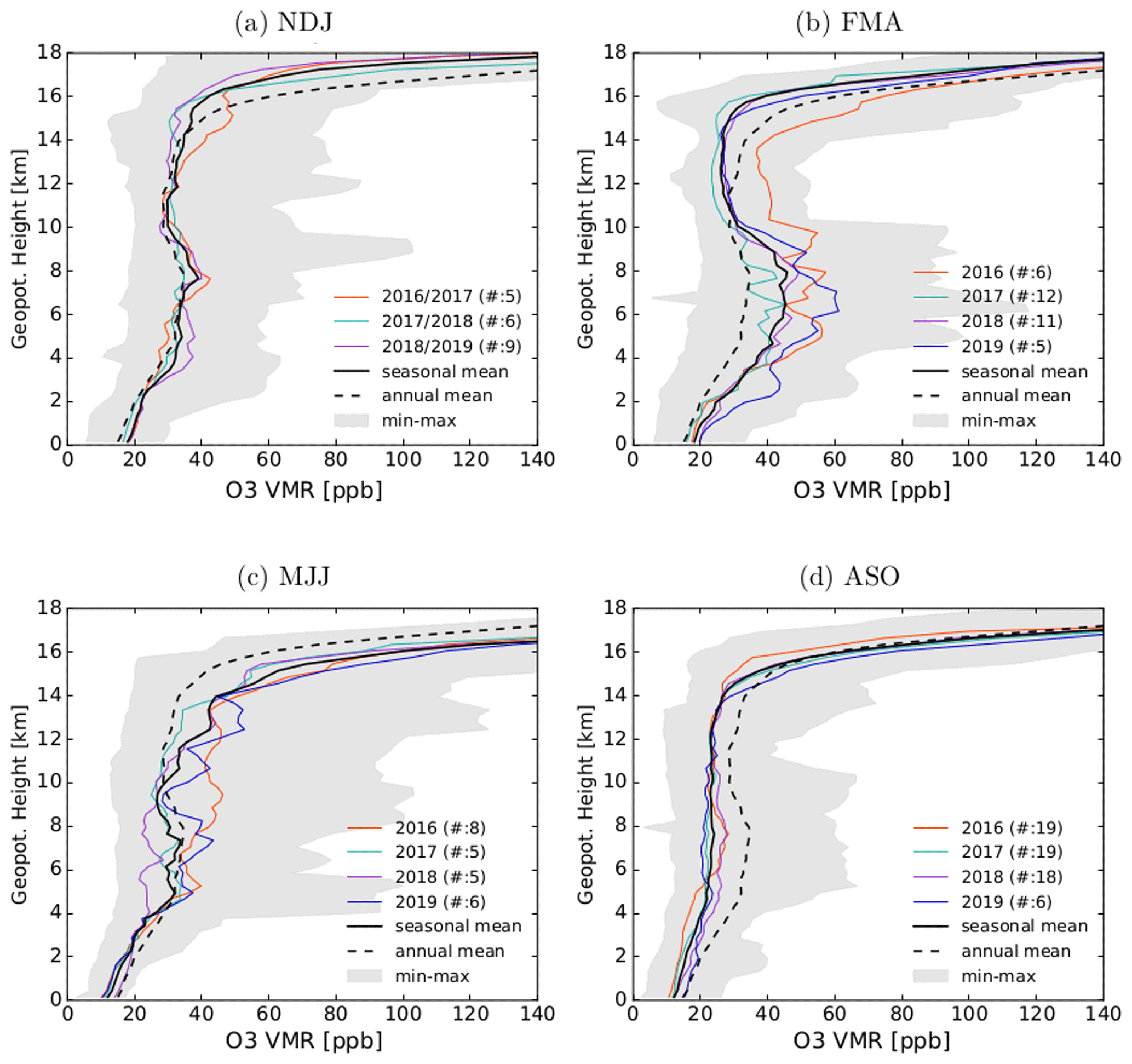
Figure A1 Variability of seasonal mean O₃ VMR profiles for Palau (solid black lines) in comparison to the long-term annual mean (dashed black line) in individual panels per season (a–d), all excluding the El Niño 2016 event, i.e., starting August 2016; the shaded grey area encloses all observations, minimum to maximum; thin colored lines indicate seasonal means per year; and the number (#) of profiles included in the calculations is given in brackets (cf. Fig. 6).

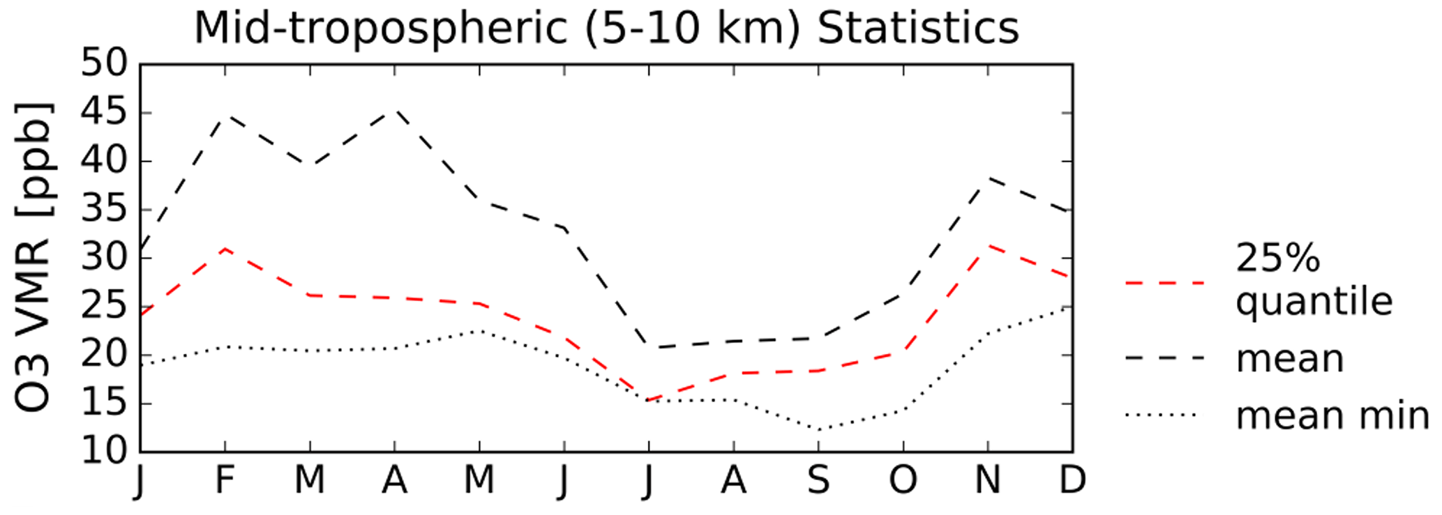
Figure A2 Statistical O₃ VMR measures for the 5–10 km altitude range highlighting the minimum O₃ season: monthly means from individual soundings' 25 % quantiles (dashed red line), mean (dashed black line) and minimum (dotted black line).

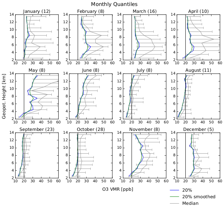
Figure A3 Monthly O₃ VMR statistics for Palau free tropospheric profiles as a function of altitude: 20th quantile (Q20) in blue, vertically smoothed using exponentially weighted averages in green, median in grey and central 66.6 % range in grey horizontal bars. The number of included individual profiles is given in brackets, and for orientation 20 ppb O₃ VMR is marked as a vertical black line (cf. Figs. 4 and A4).

Figure A4 Monthly RH statistics for Palau free tropospheric profiles as a function of altitude: 83.3th quantile (Q83) in blue. For more details, see Fig. A3. The 45 % RH is highlighted by a vertical black line (cf. Figs. 4 and A3).

Figure A5 Seasonal free-tropospheric (3–14 km) relation between tracer anomalies ΔO₃ VMR and ΔRH for November–December–January (NDJ) (a) and May–June–July (MJJ) (b), with colors according to Fig. 6. For more details, see Figs. 8 and 7.

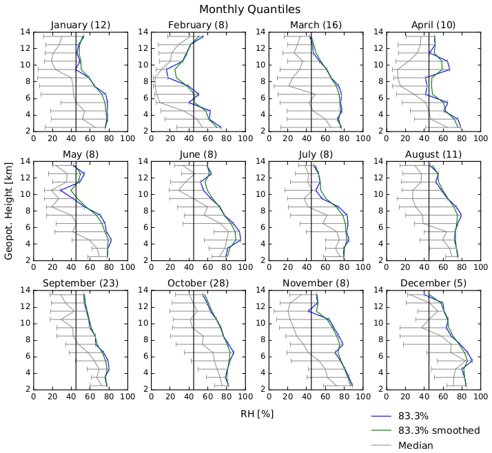
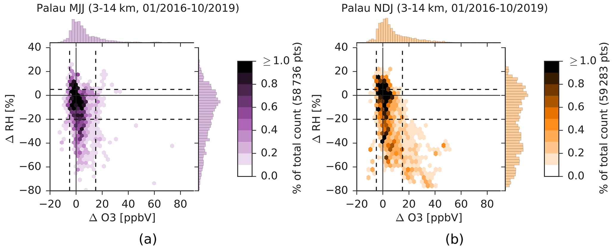
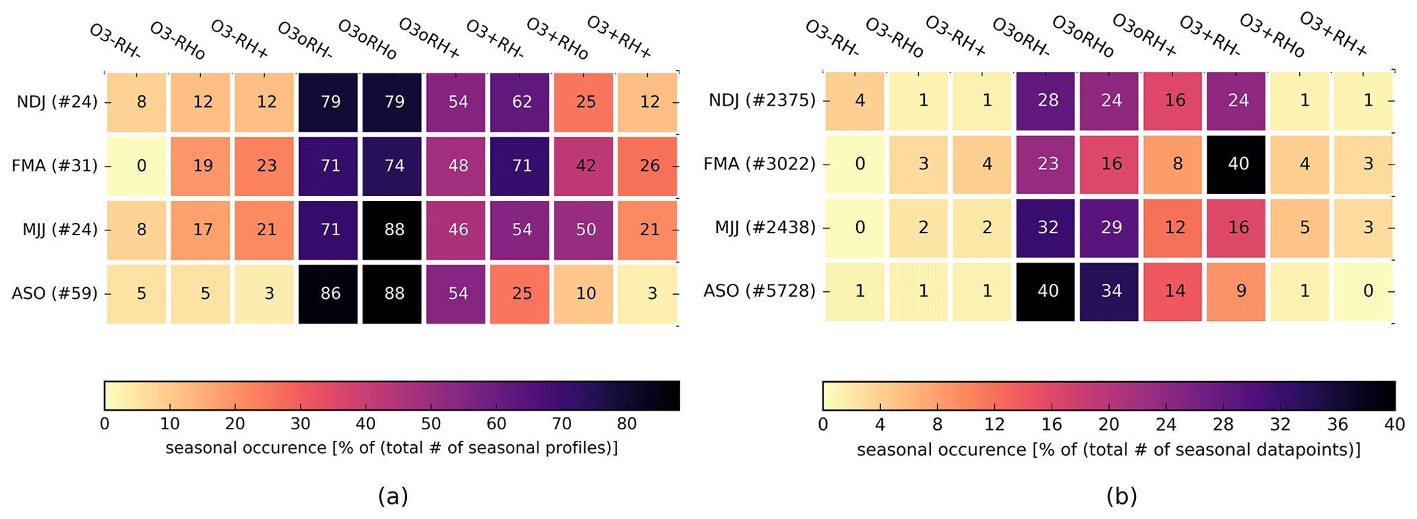
Figure A6 Heat map for the seasonal occurrence of air mass anomaly categories $\mathrm{\Delta }{\mathrm{O}}_{\mathrm{3}}/\mathrm{\Delta }$RH based on the definition given in Sect. 3.1.3 and presented in Fig. 7 for Palau observations in the 5–10 km altitude range (trajectory dataset, see Sect. 2). Panel (a) shows the occurrence relative to the total number (#) of seasonal profiles, while panel (b) shows the occurrence relative to the total number of all data points within the season. Total numbers are given in brackets per season.

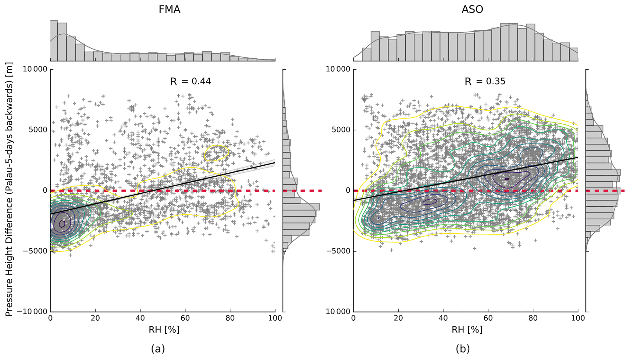
Figure A7 Relative humidity (RH) from observations above Palau versus difference in pressure altitude (between measurement date in Palau and 5 d before measurement) inferred from the backward trajectory analysis for the seasons FMA (a) and ASO (b). Grey “+” indicate individual measurements from the trajectory dataset, colored contours show the distribution density, the black line indicates a fit by linear regression with a grey shaded 95 % confidence interval, and the dashed red line highlights the zero line for the altitude difference with positive values indicating ascent and negative values descent towards Palau. The correlation coefficient R is shown in the plot. The marginal plots show univariate histograms and kernel density estimated curves.

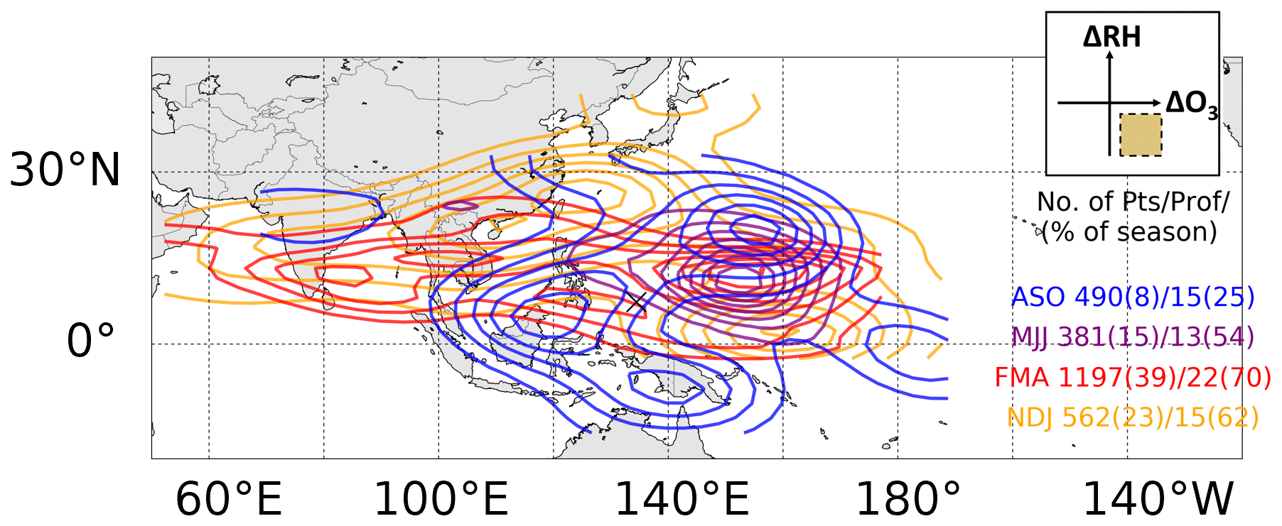
Figure A8 Seasonal distributions of the location of ΔO₃+ΔRH− air masses 5 d before their measurement in Palau in the 5–10 km altitude range inferred from trajectories, according to the definition shown in Fig. 7. The numbers in the plot show, from left to right, absolute number of individual air masses (trajectories) per season and as percentage per season in brackets, absolute number of profiles per season and as percentage per season in brackets. Differences to numbers shown in Fig. A6 due to rounding differences; see Fig. 6 for seasons.

Appendix B: Statistical averages

There are different ways to derive a climatological seasonal average and choosing the best-suited definition is not trivial with our given dataset. Data from an individual sounding are first averaged in 300 m height bins using an arithmetic mean (hereafter referred to as “mean”), which essentially complies with the vertical measurement resolution, introducing only a slightly greater degree of smoothing (cf. Müller et al., 2024). In the following temporal binning, the order of required steps must be considered as they lead to different values in our time series. There are four different possible sequences for (i) monthly, (ii) seasonal and (iii) annual averaging (Müller, 2020). In our case, we chose to first directly average individual profiles x_i(m,y) of month m of all years y to a climatological month mean, climmonmean(m), then to a climatological season mean over all years, climseasmean(s):

$$\begin{array}{}\text{(B1)}& {\displaystyle }\mathrm{climmonmean}\left(m\right)={\displaystyle \frac{\mathrm{1}}{\sum _{y=\mathrm{1}}^{Y}N(m,y)}}\times \sum _{y=\mathrm{1}}^Y\sum _{i=\mathrm{1}}^{N(m,y)}{x}_i(m,y),\text{(B2)}& {\displaystyle }\mathrm{climseasmean}\left(s\right)={\displaystyle \frac{\mathrm{1}}{M\left(s\right)}}\times \sum _{i=\mathrm{1}}^{M\left(s\right)}\mathrm{climmonmean}\left(i\right),\end{array}$$

with M(s) as the months in season s, N(m,y) as the number of profiles in month m of year y and Y as the number of years. climseasmean (s) will not overestimate single months with very few and/or outlying profiles, assuming the interannual variability of the months is small compared to variations between different months.