Abrupt excursions in water vapor isotopic variability at the Pointe Benedicte observatory on Amsterdam Island

In order to complement the picture of the atmospheric water cycle in the Southern Ocean, we have continuously monitored water vapor isotopes since January 2020 on Amsterdam Island in the Indian Ocean. We present here the first 2-year long water vapor isotopic record at this site. We show that the water vapor isotopic composition largely follows the water vapor mixing ratio, as expected in marine boundary layers. However, we detect 11 periods of a few days where there is a strong loss of correlation between water vapor δ¹⁸O and water vapor mixing ratio as well as abrupt negative excursions of water vapor δ¹⁸O. These excursions often occur toward the end of precipitation events. Six of these events show a decrease in gaseous elemental mercury, suggesting subsidence of air from a higher altitude.

Our study aims to further explore the mechanism driving these negative excursions in water vapor δ¹⁸O. We used two different models to provide a data–model comparison over this 2-year period. While the European Centre Hamburg model (ECHAM6-wiso) at 0.9° was able to reproduce most of the sharp negative water vapor δ¹⁸O excursions, hence validating the physics process and isotopic implementation in this model, the Laboratoire de Météorologie Dynamique Zoom model (LMDZ-iso) at 2° (3°) resolution was only able to reproduce seven (one) of the negative excursions, highlighting the possible influence of the model resolution for the study of such abrupt isotopic events. Based on our detailed model–data comparison, we conclude that the most plausible explanations for such isotopic excursions are rain–vapor interactions associated with subsidence at the rear of a precipitation event.

1 Introduction

The main sources of uncertainty in the atmospheric components of Earth system models for future climate projections are associated with complex atmospheric processes, particularly those related to water vapor and clouds (Arias et al., 2021; Sherwood et al., 2014). Decreasing these uncertainties is of vital interest as the hydrological cycle is a fundamental element of the climate system because it allows us, via the transport of water vapor, to ensure Earth's thermal balance.

Stable water isotopes are a useful tool for studying the influence of dynamical processes on the water budget at various spatial and temporal scales. They provide a framework for analyzing moist processes over a range of timescales from large-scale moisture transport to cloud formation, precipitation, and small-scale turbulent mixing (Bailey et al., 2023; Dahinden et al., 2021; Galewsky et al., 2016; Thurnherr et al., 2020).

The relative abundance of heavy and light isotopes in different water reservoirs is altered during phase change processes due to isotopic fractionation (caused by a difference in saturation vapor pressure and molecular diffusivity in the air and the ice). Each time a phase change occurs, the relative abundance of water vapor isotopes is altered. We express the abundance of the heavy isotopes D and ¹⁸O with respect to the number of light isotopes H and ¹⁶O, respectively, in the water molecules through the notation δ:

$$\begin{array}{}\text{(1)}& {\displaystyle }{\mathit{\delta }}^{\mathrm{18}}\mathrm{O}=\left({\displaystyle \frac{{\left({}^{\mathrm{18}}\mathrm{O}{/}^{\mathrm{16}}\mathrm{O}\right)}_{\mathrm{Sample}}}{{\left({}^{\mathrm{18}}\mathrm{O}{/}^{\mathrm{16}}\mathrm{O}\right)}_{\mathrm{VSMOW}}}}-\mathrm{1}\right)\times \mathrm{1000},\text{(2)}& {\displaystyle }\mathit{\delta }\mathrm{D}=\left({\displaystyle \frac{{\left(D/H\right)}_{\mathrm{Sample}}}{{\left(D/H\right)}_{\mathrm{VSMOW}}}}-\mathrm{1}\right)\times \mathrm{1000},\end{array}$$

where (¹⁸O $/$ ¹⁶O) and ($D/H$) represent the isotopic ratios of oxygen and hydrogen atoms in water and VSMOW (Vienna Standard Mean Ocean Water) is an international reference standard for water isotopes.

There are two types of isotopic fractionation: equilibrium fractionation, which is caused by the difference in saturation vapor pressure of different isotopes, and non-equilibrium fractionation, which occurs due to molecular diffusion (e.g., during ocean evaporation in an undersaturated atmosphere or snowflake condensation in an oversaturated atmosphere). In the water vapor above the ocean, the proportion of non-equilibrium fractionation and hence diffusive processes can be estimated by the deuterium excess, a second-order isotopic variable denoted “d-excess” and defined as (Dansgaard, 1964)

$$\begin{array}{}\text{(3)}& \text{d-excess}=\mathit{\delta }\mathrm{D}-\mathrm{8}\times {\mathit{\delta }}^{\mathrm{18}}\mathrm{O}.\end{array}$$

In recent years and thanks to the development of optical spectroscopy enabling continuous measurements of water isotope ratios in water vapor, an increasing number of studies have focused on the use of water vapor stable isotopes to document the dynamics of the water cycle over synoptic weather events, such as cyclones, cold fronts, atmospheric rivers (Aemisegger et al., 2015; Ansari et al., 2020; Bhattacharya et al., 2022; Dütsch et al., 2016; Graf et al., 2019; Lee et al., 2019; Munksgaard et al., 2015; Tremoy et al., 2014), or water cycle processes such as evaporation over the ocean or deep convection (Benetti et al., 2015; Bonne et al., 2019). Several instruments have been installed either at observatory stations (e.g., Aemisegger et al., 2012; Guilpart et al., 2017; Leroy-Dos Santos et al., 2020; Steen-Larsen et al., 2013; Tremoy et al., 2012), on boats (e.g., Benetti et al., 2014; Thurnherr et al., 2020), or on aircraft (Henze et al., 2022). In the aforementioned studies, the interpretation of the isotopic records is often performed using a hierarchy of isotopic models, from conceptual models (Rayleigh type) to general circulation models or regional weather prediction models equipped with water isotopes (Ciais and Jouzel, 1994; Markle and Steig, 2022; Risi et al., 2010; Werner et al., 2011). Such data comparisons enable one to test the performances of the models either in the simulation of the dynamics of the atmospheric water cycle or in the implementation of the water isotopes. Our study is part of these dynamics analyses and aims at improving the documentation of the climate and atmospheric water cycle in the southern Indian Ocean, a region which has been poorly documented until now.

Over the previous years, we installed three water vapor analyzers on La Réunion at the Maïdo observatory (21.079° S, 55.383° E; 2160 m) (Guilpart et al., 2017) and in Antarctica (Dumont d'Urville – 66.663° S, 140° E; 202 m; Concordia – 75.1° S, 123.333° E; 3233 m; Bréant et al., 2019; Casado et al., 2016; Leroy-Dos Santos et al., 2021). These instruments have been used for the following purposes. They document the diurnal variability of the isotopic signal with the influence of the subtropical westerly jet on the water isotopic signal at night as well as the cyclonic activity on La Réunion. In Antarctica, the records have shown a strong influence of katabatic winds on the isotopic composition of water vapor (Bréant et al., 2019). In order to complete the picture of the atmospheric water cycle over the Indian basin of the Southern Ocean already measured by these three analyzers, we installed a new water vapor isotopic analyzer at mid-latitude in the southern Indian Ocean on Amsterdam Island (Fig. 1) in November 2019. Amsterdam Island is one of the very rare atmospheric observatories in the Southern Hemisphere. Moreover, the southern Indian Ocean is a significant moisture source of Antarctic precipitation, notably in the region encompassing the Dumont d'Urville and Concordia stations (Jullien et al., 2020; Wang et al., 2020).

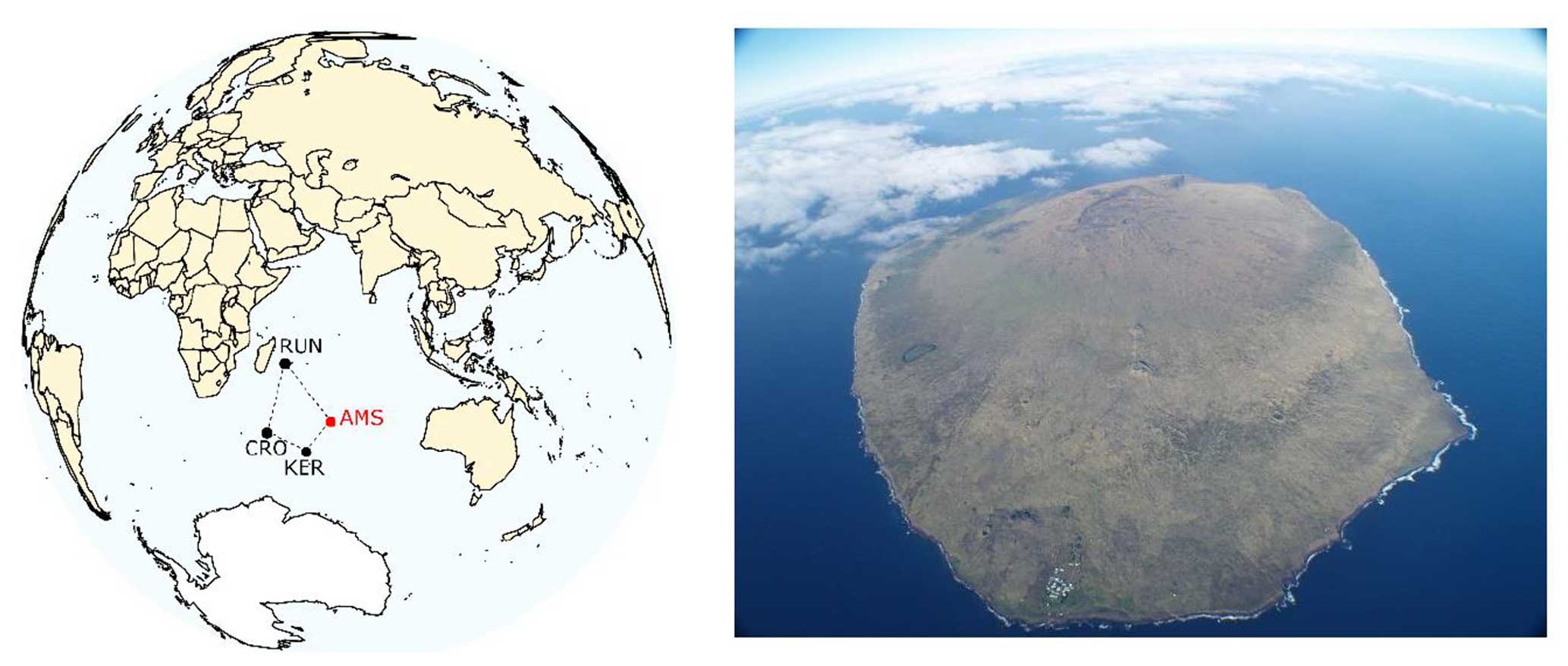
Figure 1 Location (left) and picture (right) of Amsterdam Island. CRO: Crozet islands; RUN: La Réunion; KER: Kerguelen island; AMS: Amsterdam Island. Picture credit: left – from Olivier Magand adapted from Angot et al. (2016); right – photo taken by Olivier Magand.

The objective of this study is to provide the first analyses of isotopic records (vapor and precipitation) on Amsterdam Island, with a comparison of meteorological data and environmental data collected in parallel at the Amsterdam Island observatory (e.g., atmospheric mercury) to help with the interpretation of isotopic records. Indeed, previous studies have shown that gaseous elemental mercury decreases with increasing altitude in marine environments, suggesting that gaseous elemental mercury can be used as a tracer of subsidence of air from high altitudes (e.g., Koenig et al., 2023). This study includes analyses of meteorological maps, back trajectories, and outputs from general circulation models equipped with water isotopes. After a description of the different records over the years 2020 and 2021, model simulations, and back trajectories, we focus on some low-pressure events associated with a strong negative excursion of δ¹⁸O_v over a few days and a decoupling between δ¹⁸O_v and humidity. These events are then used for evaluation of atmospheric components of Earth system models equipped with water isotopes.

2 Methods

2.1 Site

Labeled a global site for the Global Atmosphere Watch World Meteorological Organization, Amsterdam Island (37.7983° S, 77.5378° E) is a remote and very small island of 55 km² with a population of about 30 residents, located in the southern Indian Ocean at 3300 and 4200 km downwind from the nearest countries, Madagascar and South Africa, respectively (Sprovieri et al., 2016). The climate is temperate and generally mild with frequent presence of clouds (the average total sunshine hours is 1581 h yr⁻¹ over the period 1981–2010 from Météo-France data). Seasonal boundaries are defined as follows: winter from July to September and summer from December to February, in line with previous studies (Sciare et al., 2009). The average temperature is lower in winter compared to summer (10.5 °C vs. 15 °C), while the relative humidity and wind speed remain high (50 %–85 % and 5 m s⁻¹–15 m s⁻¹, respectively) most of the year without a clear seasonal cycle.

Numerous atmospheric compounds and meteorological parameters are and have been continuously monitored at the site since 1960 (Angot et al., 2014; El Yazidi et al., 2018; Gaudry et al., 1983; Gros et al., 1999, 1998; Polian et al., 1986; Sciare et al., 2000, 2009; Slemr et al., 2015, 2020). In particular, the Amsterdam Island (AMS) site hosts several dedicated atmospheric observation instruments, notably at the Pointe Bénédicte atmospheric observatory (70 m above sea level), where greenhouse gas concentrations and mercury (Hg) are monitored. Hg species have been continuously measured since 2012.

2.2 Long-term measurements

2.2.1 Meteorological measurements

One meteorological station has been installed at the top of an observation mast (25 m above ground level, hence 95 m above sea level) at the Pointe Bénédicte observatory since 1980 (data used during this study). Wind speed and direction, atmospheric pressure, air temperature, and relative humidity data are currently obtained at 1 min resolution. Another meteorological station is based on the island and is operated by Météo-France at Martin-de-Viviès life base around 27 m above sea level and about 2 km east of the Pointe Bénédicte observatory collecting air temperature, humidity, precipitation, wind speed and direction, pressure, and solar radiation.

2.2.2 Gaseous elemental mercury (GEM)

Atmospheric GEM measurements have been conducted since 2012 in the framework of the IPEV GMOStral-1028 observatory program at the Pointe Benedicte atmospheric research facility (Magand et al., 2022). GEM is continuously measured (15 min data frequency acquisition) using a Tekran 2537 A/B instrument model (Angot et al., 2014; Li et al., 2023; Slemr et al., 2015, 2020; Sprovieri et al., 2016). The measurement is based on mercury enrichment on a gold cartridge, followed by thermal desorption and detection by cold vapor atomic fluorescence spectroscopy (Bloom and Fitzgerald, 1988; Fitzgerald and Gill, 1979). Concentrations are expressed in nanograms per cubic meter under standard temperature and pressure conditions (273.15 K and 1013.25 hPa) with an instrumental detection limit below 0.1 ng m⁻³ and a GEM average uncertainty value around 10 % (Slemr et al., 2015). The instrument is automatically calibrated following a strict procedure adapted from that of Dumarey et al. (1985). Ambient air is sampled at 1.2 L min⁻¹ through a heated (50 °C) and UV-protected PTFE (polytetrafluoroethylene) sampling line, with an inlet installed outside, 6 m above ground level (76 m above sea level). The air is filtered through two 0.45 µm pore size polyethersulfone and one PTFE 47 mm diameter filters before entering in Tekran to prevent the introduction of any particulate material into the detection system as well as to capture any gaseous oxidized mercury or particulate-bound mercury species, ensuring that only GEM is sampled. To ensure the comparability of mercury measurements around the world, the instrument is operated according to the Global Mercury Observation System standard operating procedures (Sprovieri et al., 2016; Steffen et al., 2012).

In this study, and even though long-range transport and a variable tropopause height may modulate the signal, atmospheric GEM is used as a potential tracer of stratosphere-to-troposphere intrusion and/or subsidence of upper-tropospheric air (above 5–6 km), which may impact the atmospheric records at the Pointe Benedicte observatory, where marine boundary layer air is collected most of the time (Angot et al., 2014; Slemr et al., 2015, 2020; Sprovieri et al., 2016). Mercury in the atmosphere consists of three forms: GEM as defined above, gaseous oxidized mercury, and particulate-bound mercury. GEM, the dominant form of atmospheric mercury, is ubiquitous in the atmospheric reservoir and originates from a multitude of anthropogenic and natural sources (Edwards et al., 2021; Gaffney and Marley, 2014; Gustin et al., 2020; Gworek et al., 2020). Near the surface (marine or terrestrial boundary layer) and outside polar regions, gaseous oxidized mercury and particulate-bound mercury represent only a few percent of the total atmospheric mercury (Gustin and Jaffe, 2010; Gustin et al., 2015; Swartzendruber et al., 2006). Chemical cycling and the spatiotemporal distribution of mercury in the air are still poorly understood regardless of the atmospheric layer considered (surface, mixed or free troposphere, stratosphere), and complete GEM oxidation schemes remain unclear (Shah et al., 2021, and associated references). Still, several studies provided evidence that the vertical distribution of atmospheric mercury measurements from the boundary layer to the lower or upper troposphere and stratosphere shows a decreasing trend in GEM concentration with increasing altitude, in parallel with an increase in the concentration of divalent mercury resulting from GEM oxidation mechanisms (Brooks et al., 2014; Faïn et al., 2009; Fu et al., 2016; Koenig et al., 2023; Lyman and Jaffe, 2012; Murphy et al., 2006; Swartzendruber et al., 2006, 2008; Sheu et al., 2010; Talbot et al., 2007). The identification of such observational processes (lower concentration of GEM in high-altitude air masses compared to those in the marine boundary layer ones) is used here to help characterize possible intrusions of high-altitude air masses at the low-altitude Pointe Benedicte observatory.

2.3 Water vapor isotopic measurements

The near-surface water vapor δ¹⁸O and δD (hereafter δ¹⁸O_v and δD_v, ‰, vs. SMOW and enabling us to calculate water vapor d-excess_v as d-excess_v=δD${}_{\mathrm{v}}-\mathrm{8}\times {\mathit{\delta }}^{\mathrm{18}}$O_v). The water vapor mixing ratio (q_v, ppmv) has been measured continuously since November 2019. The measurements have been made with a Picarro Inc. instrument (L2130-i model) based on wavelength-scanned cavity ring-down spectroscopy. The instrument is installed in a temperature-controlled room at the Amsterdam Island observatory, and the sampling of water vapor is done outside at ∼6 m above ground level (or 76 m above sea level) through a 5 m long inlet tube made of PFA (perfluoroalkoxy alkanes) and heated at 40 °C.

The calibration of the water vapor mixing ratio was performed in the laboratory before sending the instrument to Amsterdam Island. In the field, we found excellent agreement between the mixing ratio measured by the Picarro instrument and the mixing ratio measured by the weather station (the difference between the two records always stays below 2 %, and there is no systematic shift between the two records).

The calibration of the water isotopic data is performed in several steps following previous studies (Leroy-Dos Santos et al., 2020; Tremoy et al., 2011) and using a standard delivery module by Picarro. First, we quantified the influence of the water vapor mixing ratio on the water isotope ratios. This effect is large at very low humidity (Leroy-Dos Santos et al., 2021). It can also depend on the isotopic composition of the standard water (Weng et al., 2020). Here, we introduced two different water standards, EPB-AMS and GREEN-AMS, with respective values of (−5.66 ‰, −47.31 ‰) and (−32.65 ‰, −263.76 ‰) for the couple (δ¹⁸O, δD) which encompass the isotopic values observed on site. While we would expect a constant null value for (δ¹⁸O_measured−δ¹⁸O_standard) in Fig. 2 because we always inject the same water standards, the measured δ¹⁸O values of both the EPB-AMS and GREEN-AMS standards in fact decrease with increasing humidity at the same amplitude. The (δD_measured−δD_standard) displayed in Fig. 2 also shows variations, but in contrast to the relative evolution of δ¹⁸O with respect to the water vapor mixing ratio, the δD measurements of the EPB-AMS and GREEN-AMS standards exhibit different behavior: the δD of EPB-AMS increases by 1.5 ‰, and the δD of GREEN-AMS decreases by 2.5 ‰ over the same 6000–24 000 ppmv range for the water vapor mixing ratio q_v.

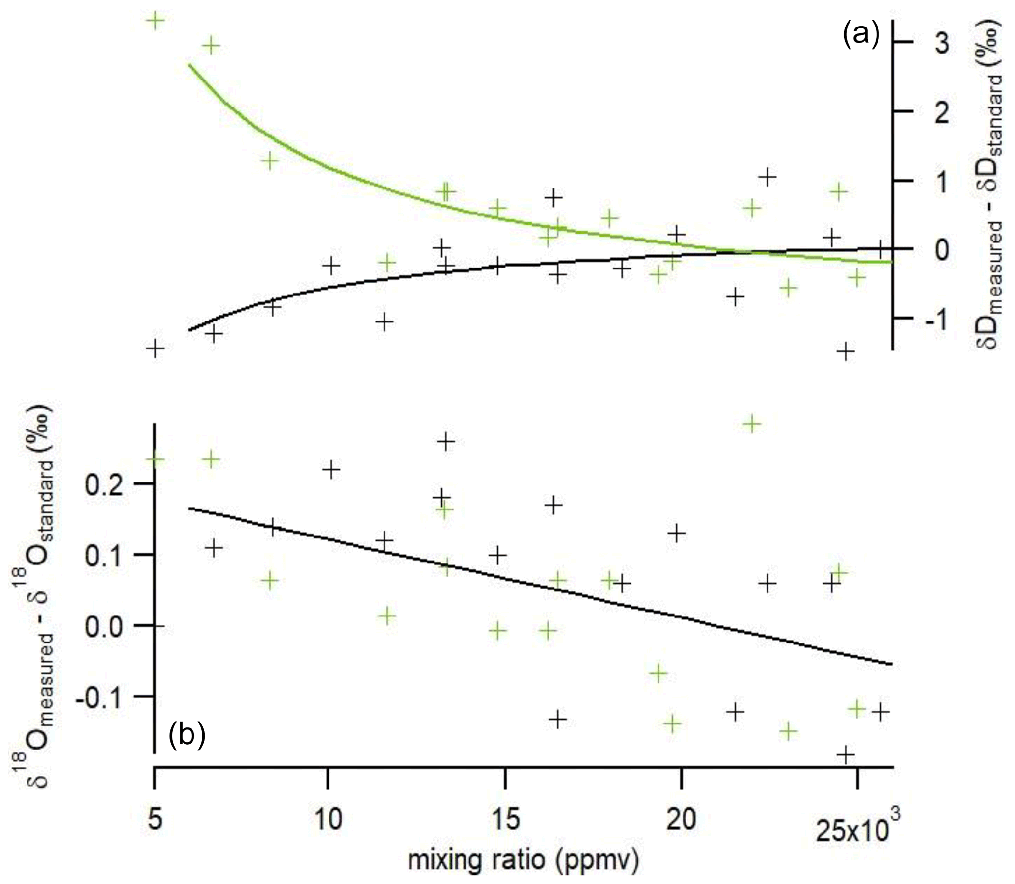
Figure 2 Influence of the water vapor mixing ratio on measured δD (a) and δ¹⁸O (b) (anomaly from the true value of the standard). The results are shown for two different standards (GREEN_AMS in green and EPB_AMS in black). The crosses indicate the data obtained with the setup, and the solid lines are the best regression curves (same curve for δ¹⁸O for both standards).

As a consequence, the raw δ¹⁸O_v measurements are corrected with the following regression:

$$\begin{array}{}\text{(4)}& {\mathit{\delta }}^{\mathrm{18}}{\mathrm{O}}_{\mathrm{v},\mathrm{corr}}={\mathit{\delta }}^{\mathrm{18}}{\mathrm{O}}_{\mathrm{v},\mathrm{measured}}+{\mathrm{1.1.10}}^{-\mathrm{5}}\times q+\mathrm{0.232}.\end{array}$$

For the correction of the raw δD_v, we use two different regression splines for EPB-AMS and GREEN-AMS (see Fig. 2):

$$\begin{array}{}\text{(5)}& {\displaystyle }\mathit{\delta }{\mathrm{D}}_{\text{EPB-AMS,corr}}=\mathit{\delta }{\mathrm{D}}_{\text{EPB-AMS,measured}}+{\displaystyle \frac{\mathrm{9300}}{q}}-\mathrm{0.383},\text{(6)}& {\displaystyle }\mathit{\delta }{\mathrm{D}}_{\text{GREEN-AMS,corr}}=\mathit{\delta }{\mathrm{D}}_{\text{GREEN-AMS,measured}}-{\displaystyle \frac{\mathrm{22400}}{q}}+\mathrm{1.05}.\end{array}$$

The raw δD_v are thus weighted-corrected according to their distance to the EPB_AMS and GREEN_AMS splines as follows:

$$\begin{array}{}\text{(7)}& \begin{array}{rl}\mathit{\delta }{\mathrm{D}}_{\mathrm{v},\mathrm{corr}}& =\mathit{\delta }{\mathrm{D}}_{\text{GREEN-AMS,corr}}\\ & +{\displaystyle \frac{\mathit{\delta }{\mathrm{D}}_{\mathrm{v},\mathrm{measured}}-\mathit{\delta }{\mathrm{D}}_{\text{GREEN-AMS,measured}}}{\mathit{\delta }{\mathrm{D}}_{\text{EPB-AMS,measured}}-\mathit{\delta }{\mathrm{D}}_{\text{GREEN-AMS,measured}}}}\\ & \times (\mathit{\delta }{\mathrm{D}}_{\text{EPB-AMS,corr}}-\mathit{\delta }{\mathrm{D}}_{\text{GREEN-AMS,corr}}).\end{array}\end{array}$$

This first calibration step (correction from the influence of the mixing ratio on the isotopic composition) has been performed every year over the whole range of mixing ratio values and provided very similar results from one year to the other. The second calibration step consists of the injection of the same two isotopic standards every 47 h at a water vapor mixing ratio of 13 000 ppmv to correct for any long-term drift. The correction associated with this drift is less than 0.4 ‰ for δ¹⁸O and 2.5 ‰ for δD over the 2 years of measurements.

Precipitation was also sampled on a weekly basis in a rain gauge filled with paraffin oil, which permits us to have measurements of water isotopic composition in the precipitation on a weekly basis. The water samples are then sent for analyses to the LSCE (Laboratoire des Sciences du Climat et de l'Environnement) and measured with an L2130-i isotopic analyzer by Picarro. The uncertainty associated with this series of measurements is ±0.15 ‰ for δ¹⁸O and ±0.7 ‰ for δD, leading to an uncertainty of ±1.4 ‰ for d-excess.

2.4 Back trajectories: FLEXPART

The origin and trajectory of air masses were calculated by FLEXPART, which is a Lagrangian particle dispersion model (Pisso et al., 2019). All the meteorological data used to simulate the back trajectories are taken from the ERA5 atmospheric reanalysis (Hersbach et al., 2020) with a 6-hourly resolution. The ERA5 reanalysis is carried out by the European Centre for Medium-Range Weather Forecasts (ECMWF) using its Earth system model IFS (Integrated Forecasting System), cycle 41r2. For a few selected events, we used FLEXPART to calculate back trajectories over 5 d with 1000 launches of neutral particles (sensitivity test) of inert air tracers released randomly (volume of 0.1° × 0.1° × 100 m) every 3 h at 100 m above sea level (Leroy-Dos Santos et al., 2020) centered around the coordinates of Amsterdam Island. The results of the FLEXPART back trajectories are then displayed as particle probability density as well as through the location of their humidity-weighted averages.

2.5 General atmospheric circulation model equipped with water stable isotopes

2.5.1 LMDZ-iso model (Laboratoire de Météorologie Dynamique Zoom model equipped with water isotopes)

LMDZ-iso (Risi et al., 2010) is the isotopic version of the atmospheric general circulation model LMDZ6 (Hourdin et al., 2020). We have used LMDZ-iso version 20230111.trunk with the physical package NPv6.1, identical to the atmospheric setup of IPSL-CM6A (Boucher et al., 2020) used for phase 6 of the Coupled Model Intercomparison Project (CMIP6, Eyring et al., 2016). We performed two simulations, one at very low horizontal resolution (VLR, 3.75° in longitude and 1.9° in latitude, 96×95 grid cells) and the second at low horizontal resolution (LR, 2.0° in longitude and 1.67° in latitude, 144×142 grid cells). Both simulations have 79 vertical levels, and the first atmospheric level is located around 10 m above ground level. The LMDZ-iso 3D fields of temperature and wind are nudged toward the 6-hourly ERA5 reanalysis data with a relaxation time of 3 h. Surface ocean boundary conditions are taken from the monthly mean sea surface temperature (SST) and sea ice fields from the CMIP6 AMIP Sea Surface Temperature and Sea Ice dataset version 1.1.8 (Durack et al., 2022; Taylor et al., 2000). LMDZ-iso outputs are used at a 3-hourly resolution. Amsterdam Island (58 km²) is too small to be represented in the LMDZ-iso model.

2.5.2 ECHAM6-wiso model (European Centre Hamburg model equipped with water isotopes)

ECHAM6-wiso (Cauquoin et al., 2019; Cauquoin and Werner, 2021) is the isotopic version of the atmospheric general circulation model ECHAM6 (Stevens et al., 2013). The implementation of the water isotopes in ECHAM6 has been described in detail by Cauquoin et al. (2019) and has been updated in several aspects by Cauquoin and Werner (2021) to make the model results more consistent with the last findings based on water isotope observations (isotopic composition of snow on sea ice considered, supersaturation equation slightly updated, and kinetic fractionation factors for oceanic evaporation assumed to be independent of wind speed). We have used ECHAM6-wiso model outputs from a simulation with a T127L95 spatial resolution (0.9° horizontal resolution and 95 vertical levels). ECHAM6-wiso is thus run with a finer resolution than both LMDZ-iso simulations. The ECHAM6-wiso 3D fields of temperature, vorticity, and divergence as well as the surface pressure field were nudged toward the ERA5 reanalysis data every 6 h (Hersbach et al., 2020). The orbital parameters and greenhouse gas concentrations have been set to the values of the corresponding model year. The monthly mean sea surface temperature and sea ice fields from the ERA5 reanalysis have been applied as ocean surface boundary conditions as well as a mean δ¹⁸O of surface seawater reconstruction from the global gridded dataset of LeGrande and Schmidt (2006). As no equivalent dataset of the δD composition of seawater exists, the δD of the seawater in any grid cell has been set equal to the related δ¹⁸O composition, multiplied by a factor of 8, in accordance with the observed relation for meteoric water on a global scale (Craig, 1961). The ECHAM6-wiso simulation is described in detail and evaluated by Cauquoin and Werner (2021). ECHAM6-wiso outputs are given at a 6-hourly resolution. As for the LMDZ-iso model, Amsterdam Island (58 km²) is too small to be represented by ECHAM6-wiso.

3 Results

3.1 Data description

3.1.1 Temporal variability in the meteorological records

As mentioned earlier, there is a clear annual cycle at Amsterdam Island, as recorded in the temperature and water vapor mixing ratio for the years 2020 and 2021. The December–February period (austral summer) has the highest temperatures with an average of 15.0 °C, while in winter (July–September) the average temperature varies around 10.5 °C. In parallel, we do not see clear patterns of a diurnal cycle in the temperature record, except for some periods with a small amplitude (4–5 °C).

The impact of synoptic events at the scale of a few days is visible in the temperature and water mixing ratio with a covariation of the temperature and water vapor mixing ratio and amplitudes of up to 10 °C and more than 10 000 ppmv.

3.1.2 Temporal variability in the GEM record

Previous studies clearly showed that AMS is little influenced by anthropogenic sources of mercury and greatly influenced by the ocean surrounding the island (Angot et al., 2014; Hoang et al., 2023; Jiskra et al., 2018; Li et al., 2023; Slemr et al., 2015, 2020). Angot et al. (2014) reported mean annual GEM concentrations of about 1.03±0.08 ng m⁻³ from 2012 to 2013. These concentrations are ∼30 % lower than those measured at remote sites of the Northern Hemisphere. Over the period 2012 to 2017, Slmer et al. (2020) confirmed that higher GEM concentrations can be found during austral winter. Lower GEM values are generally observed in October and November as well as in January and February during austral summer. Using this 6-year long dataset, the mean annual GEM concentration is 1.04 ± 0.07 ng m⁻³ (annual range 1.014 to 1.080 ng m⁻³), i.e., very close to the one observed by Angot et al. (2014).

Surprisingly, unlike the 2012–2017 dataset, the GEM presented in this study did not show a significantly higher mean concentration during the austral winter months than during the summer months (Fig. 3), with consequently no discernible seasonal amplitude of GEM. On a finer timescale, the lack of a clear pattern of the GEM seasonal cycle is counterbalanced by days showing abrupt increases or decreases in concentrations. Some of the sudden GEM decreases appear concomitant with important negative peaks of several per mille in δ¹⁸O_v.

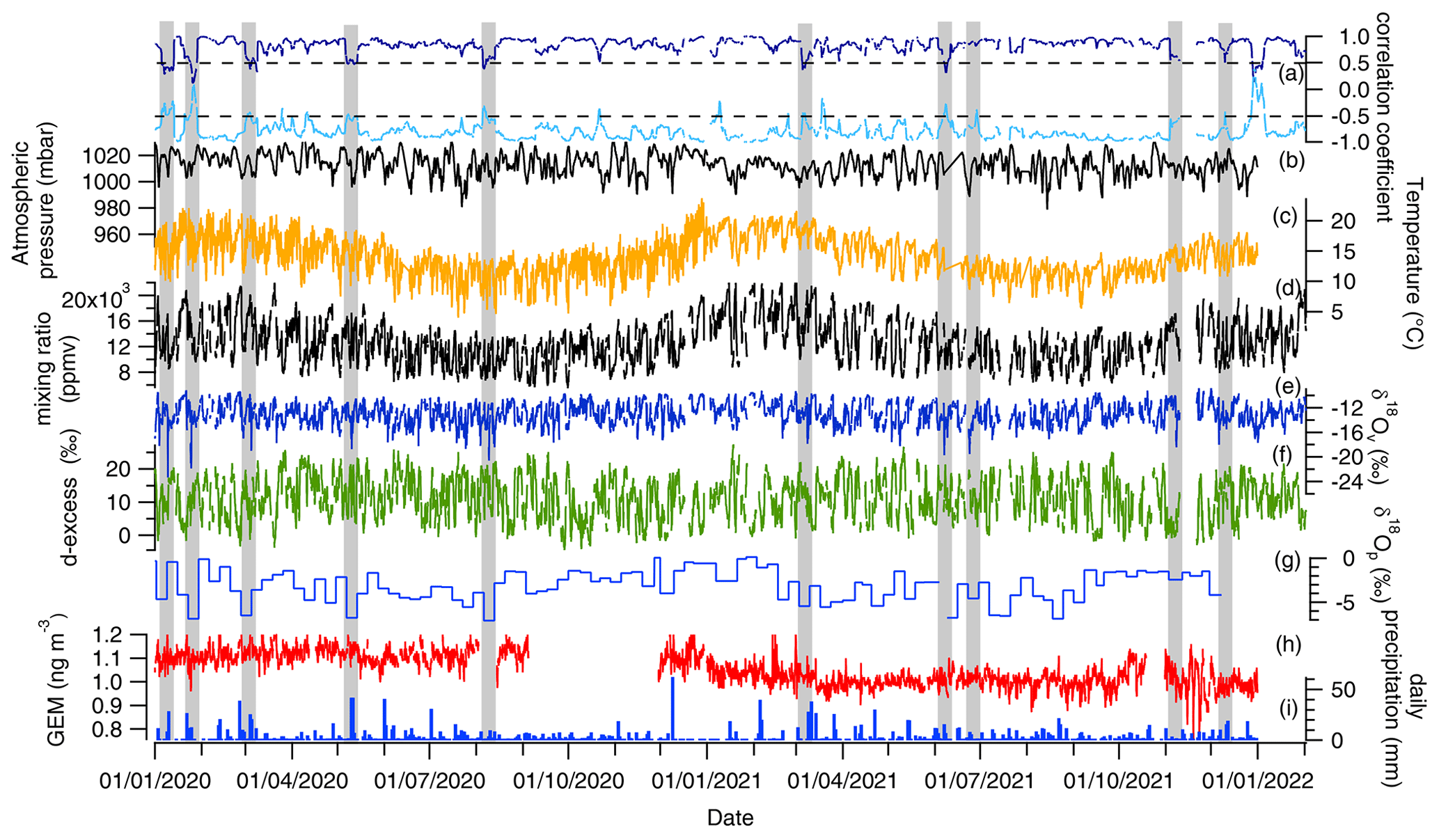
Figure 3 Meteorological, isotopic, and GEM records for the years 2020 and 2021 on the Amsterdam Island (a) correlation coefficient between δ¹⁸O_v and the mixing ratio (dark blue, top) and between δ¹⁸O_v and d-excess_v (light blue, bottom) over a moving time window of 8 d, (b) atmospheric pressure (hourly average), (c) atmospheric temperature (hourly average), (d) water vapor mixing ratio (hourly average), (e) δ¹⁸O_v (hourly average), (f) d-excess_v (hourly average), (g) δ¹⁸O of precipitation sampled on a weekly basis, (h) GEM concentration (hourly average), and (i) daily precipitation. The grey-shaded areas indicate the negative excursions in δ¹⁸O_v associated with decorrelation between the water vapor mixing ratio and δ¹⁸O_v and a correlation coefficient > −0.5 between d-excess_v and δ¹⁸O_v.

3.1.3 Temporal variability of water isotopic composition

The isotopic composition of precipitation (δ¹⁸O_p) sampled on a weekly basis displays a quite large variability (δ¹⁸O${}_{\mathrm{p}}=-\mathrm{3.06}\pm \mathrm{1.75}$ ‰, n=104) with values slightly higher during austral summer (the difference between summer and winter δ¹⁸O_p values is about 2 ‰ to 3 ‰) (Fig. 3). No significant seasonal variations are observed in the record of d-excess of precipitation (not shown).

No diurnal cycle can be detected in the δ¹⁸O_v and d-excess_v. An annual cycle is not visible either (1 ‰ difference between the summer and winter mean δ¹⁸O_v values, while the standard deviation of the entire record at 1 h resolution is 1.7 ‰). Only the synoptic-scale variability is well expressed in the records of δ¹⁸O_v and d-excess_v with an anticorrelation between both parameters when looking at the 2-year series at hourly resolution (R²= 0.61, with R² being the coefficient of determination for a linear regression). Moreover, δ¹⁸O_v is correlated most of the time with the water vapor mixing ratio (R²= 0.55 for the 2-year series at hourly resolution).

There are a few exceptions to the general correlation between the water vapor δ¹⁸O and the water vapor mixing ratio as illustrated in Fig. 3. Short periods of a few days are associated with a decrease in the correlation coefficient R estimated from the correlation between δ¹⁸O_v and q_v (R is calculated continuously from hourly records on an 8 d moving window). The periods of low R are also often characterized by a negative peak of several per mille in δ¹⁸O_v, which is not visible in the d-excess_v. During these δ¹⁸O_v excursions, the general anticorrelation between δ¹⁸O_v and d-excess_v hence also breaks down. Our study mostly focuses on the 11 most prominent abrupt events highlighted in the δ¹⁸O_v record (only 10 visible in Fig. 3 because of the scale). The 11 most abrupt events occurring when the correlation coefficient R between δ¹⁸O_v and d-excess_v is larger than −0.5 are associated with a δ¹⁸O_v negative excursion larger than 3 ‰ (at 6 h resolution) over a period of less than 24 h, the length of the event being measured between the middle slopes of the decrease and a subsequent increase in the δ¹⁸O_v. The 11 selected negative excursions occur at a rate larger than −0.5 ‰ h⁻¹, and the δ¹⁸O_v increase at the end of each excursion has an amplitude larger than half the amplitude of the corresponding initial decrease.

3.2 Model–data comparison

We selected a 3-month period (January to March 2020) for the comparison between our dataset and the outputs of the ECHAM6-wiso and LMDZ-iso models. This period has been selected for display because it encompasses 4 out the 11 negative excursions of δ¹⁸O_v, but the extended comparison over the whole 2-year period is displayed in Fig. A1. There is overall agreement between the measured and modeled δ¹⁸O_v and water vapor mixing ratio (Fig. 4). The best agreement over the 3-month series is obtained with the ECHAM6-wiso and LMDZ-iso (LR) models (R²= 0.59–0.6 and 0.87–0.90, respectively, for δ¹⁸O_v and water vapor mixing ratio series), while slightly less good agreement is observed with the VLR simulation of the LMDZ-iso model (R²= 0.49 and 0.79, respectively, for δ¹⁸O_v and the water vapor mixing ratio series). The same observation can be made of the entire 2-year time series. We also compare the precipitation amount modeled by ECHAM6-wiso and LMDZ-iso to the precipitation amount measured by the Météo-France weather station. The correlation between modeled and measured precipitation is close to zero for LMDZ-iso (R²= 0.08–0.13 for VLR–LR), while there is better agreement when comparing the measured precipitation amount to outputs of ECHAM6-wiso (R²= 0.45). Finally, when focusing on the short-term negative δ¹⁸O_v excursions (Figs. 4 and A1), they are in general more strongly expressed in the measurement time series than in the model series. Part of this disagreement can be explained by the fact that the δ¹⁸O_v record has a higher temporal resolution (1 h) than the model outputs (3 h for LMDZ-iso and 6 h for ECHAM6-wiso). However, when interpolating the δ¹⁸O_v record at a 6 h resolution (dotted dark blue), the negative excursions are still clearly visible but not captured by the LMDZ-iso model (Fig. 4 and Table 1). When looking at the whole 2-year series, the LMDZ-iso VLR simulation fails to reproduce most of these δ¹⁸O_v excursions (only the negative excursion of 3 January 2020 is reproduced), while the ECHAM6-wiso model is able to capture all the δ¹⁸O_v excursions. The LMDZ-iso LR simulation produces a negative δ¹⁸O_v excursion over many events with a significantly lower amplitude than in the data and in the ECHAM6-wiso model (Table 1).

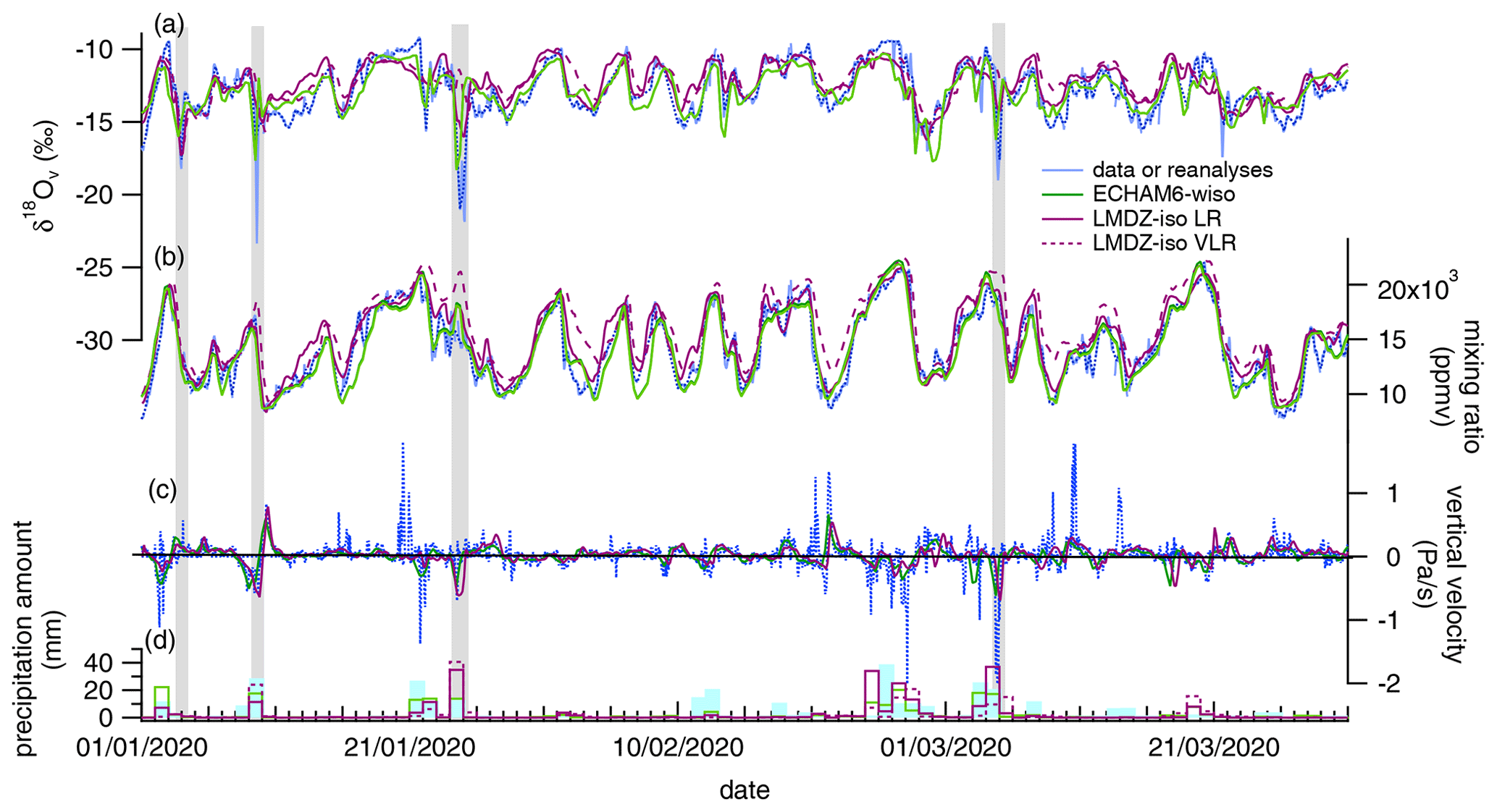
Figure 4 Model–measurement comparison (January–March 2020): (a) δ¹⁸O_v (light blue for data on hourly average, dotted dark blue for data resampled at a 6 h resolution); (b) water vapor mixing ratio from our dataset; (c) vertical velocity; (d) precipitation amount. The grey-shaded areas highlight the negative δ¹⁸O_v excursions as defined in Sect. 3.1.3 (note that in this figure the excursions of 3 and 9 January 2020 are distinct, while the distinction could not be made in Fig. 3 because of the scale).

Table 1 List of the 11 events associated with loss of correlation between δ¹⁸O_v and q_v, δ¹⁸O_v and d-excess_v, and negative excursions of δ¹⁸O_v over 2020–2021. The amplitude of the negative δ¹⁸O_v anomaly is calculated from the minimum of δ¹⁸O_v on the record at hourly resolution (at 6 h resolution). When the calculated amplitude is smaller than 1 ‰, we indicate only “–”. When the vertical velocity is between −0.25 and 0.25 Pa s⁻¹, this is indicated in the table as “∼ 0”.

4 Discussion

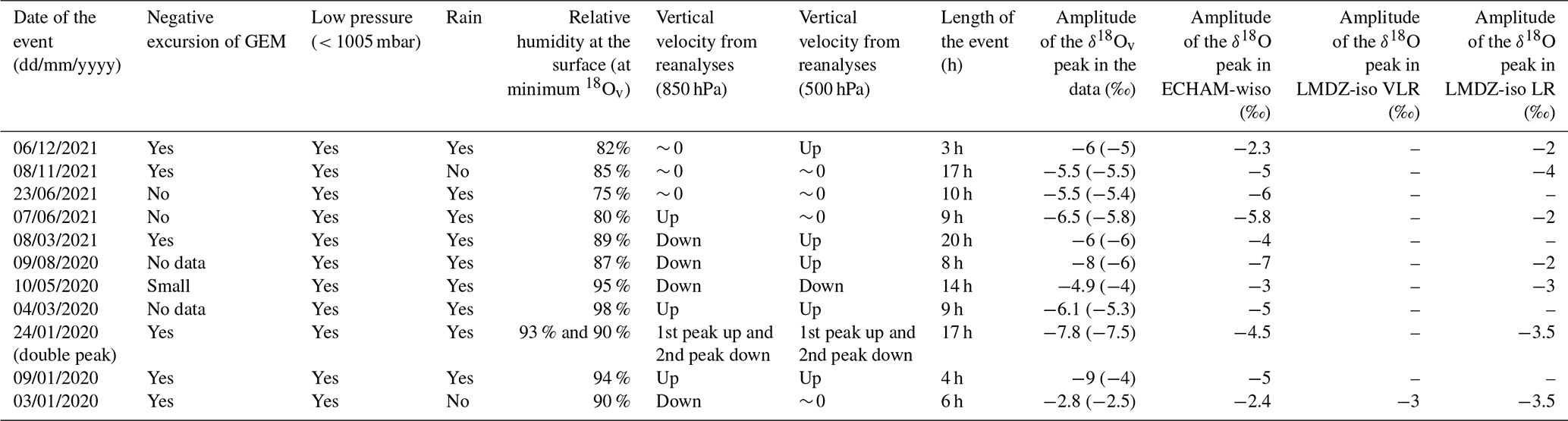
The most remarkable pattern from this 2-year series is the succession of short negative excursions of δ¹⁸O_v associated with decorrelation between δ¹⁸O_v and humidity, δ¹⁸O_v, and d-excess_v and which is highlighted with grey-shaded areas in Fig. 3, as detailed in Figs. 5 and A2 and referenced in Table 1. These negative δ¹⁸O_v excursions always occurred during low-pressure periods (atmospheric pressure below 1005 mbar), and we observe the presence of a cold front within a distance of 100 km around Amsterdam Island in a 48 h period covering the time of the event (Supplement Fig. S1). The focus on the first 3 months of the series presented in Fig. 4 shows that these events are captured by ECHAM6-wiso at 0.9° resolution but not systematically by LMDZ-iso at 2×1.67° and even less so by LMDZ-iso at 3.75×1.9° resolution. Such a mismatch makes the understanding of the processes at play during these events particularly important to investigate to further improve the performances of atmospheric general circulation models equipped with water isotopes.

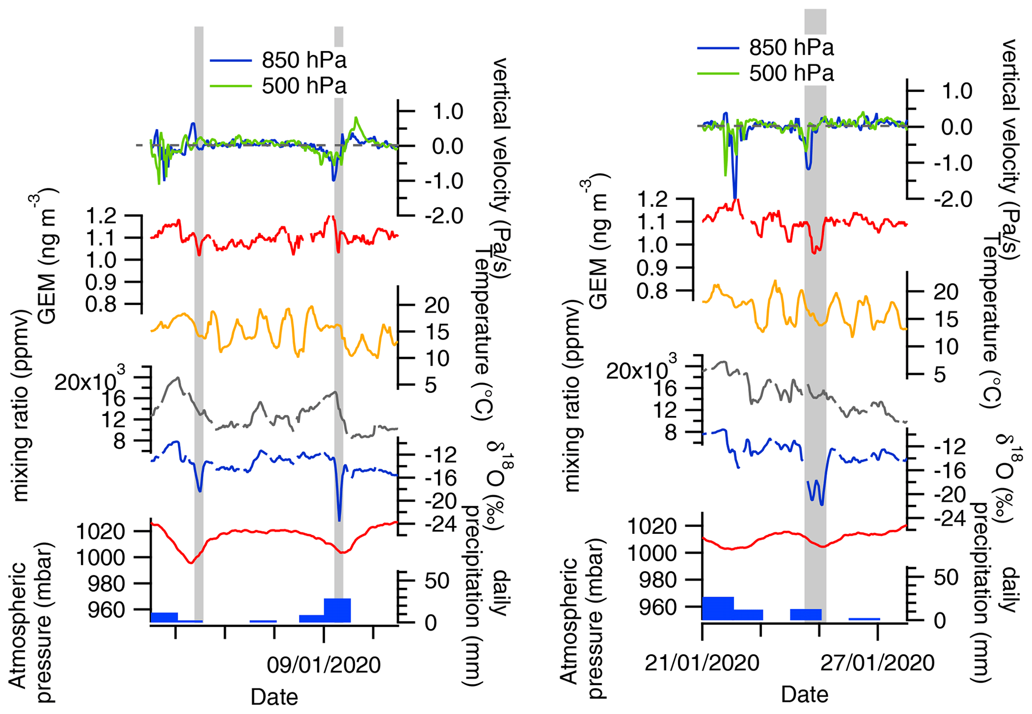
Figure 5 Evolution of the GEM, δ¹⁸O_v, water vapor mixing ratio, and meteorological parameters (surface temperature, surface atmospheric pressure, daily precipitation) measured by the Météo-France weather station and vertical velocity from the ERA5 reanalyses at 500 and 850 hPa over the three isotopic excursions of January 2020 (a, b) identified in Fig. 4. A focus on the other excursions is provided in Fig. A2.

Several hypotheses can be proposed to explain the negative excursions of δ¹⁸O_v. The beginning of these excursions is associated with a decrease in the water vapor mixing ratio and occurs in most cases during a precipitation event (Table 1). These events share similarities with negative δ¹⁸O_v and δ¹⁸O_p short events previously observed in temperate regions during a cold front passage (e.g., Aemisegger et al., 2015). Three possible processes at play to explain such events have already been listed in previous studies (e.g., Dütsch et al., 2016): (i) local interaction between the vapor and the rain droplets (rain equilibration and rain evaporation), (ii) vertical subsidence of water vapor with depleted isotopic composition, or (iii) horizontal advection through the arrival of a cold front. We explore below how we can gain information on the different processes using our dataset, back trajectories, and model–data comparison.

Figure 6 Relative evolution of q_v and δ¹⁸O_v for the different events (colors according to the date as explained in the graph) and for the entire 2-year records (grey). The solid lines are theoretical lines whose equations are detailed in Noone (2012) for different processes (re-moistening associated with exchange between rain and water vapor; Rayleigh distillation assuming that all formed condensation is removed from the cloud; a moist adiabatic process assuming that liquid condensation stays in the cloud with the water vapor; mixing of water vapor from ocean evaporation around Amsterdam Island and water vapor from the end of the Rayleigh distillation, i.e., high-altitude water vapor). The water vapor for the calculation of Rayleigh distillation and for the evaporation above the ocean has a q_v,0 of 20 000 ppmv and a δ¹⁸O_v,0 of −9.3 ‰. The vapor at the end of the distillation line has a water vapor mixing ratio of 1000 ppmv and a δ¹⁸O_v of −40 ‰.

4.1 δ¹⁸O_v–q_v relationship

First, to test the hypothesis of vapor–droplet interactions, we looked at the δ¹⁸O_v vs. q_v distribution following the approach already used by Guilpart et al. (2017) (Fig. 6). We acknowledge that our approach is crude and should be taken as a first-order approach since we can only look at the water vapor δ¹⁸O_v vs. q_v distribution in the surface layer using adapted boundary conditions, while it may be more relevant to look at this relationship in the free troposphere. In general, the δ¹⁸O_v vs. q_v evolution lies on a curve which can be explained by condensation processes (Rayleigh distillation or reversible moist adiabatic process). However, for the 11 events highlighted above, the water vapor δ¹⁸O_v vs. q_v evolution follows an evolution standing below the curve of the δ¹⁸O_v vs. q_v evolution observed for the rest of the series. Although the evolution of the water vapor δ¹⁸O_v vs. q_v is rather abrupt, there is a certain resemblance to the idealized theoretical re-moistening curve initially calculated for the free troposphere (Noone, 2012) and adapted here with initial conditions corresponding to the isotopic composition of surface water vapor. Re-moistening is described through a modification of the equilibrium fractionation coefficient between water vapor and rain (α_e), so that the effective fractionation factor is $\mathit{\alpha }=(\mathrm{1}+\mathit{\phi })\times {\mathit{\alpha }}_e$, φ being the degree to which α deviates from equilibrium. This effective fractionation coefficient is then introduced in the Rayleigh distillation equation to deduce the link between δ¹⁸O_v and the mixing ratio as

$$\begin{array}{}\text{(8)}& {\mathit{\delta }}^{\mathrm{18}}{\mathrm{O}}_{\mathrm{v}}-{\mathit{\delta }}^{\mathrm{18}}{\mathrm{O}}_{\mathrm{v},\mathrm{0}}=(\mathit{\alpha }-\mathrm{1})\times \ln (q_{\mathrm{v}}/q_{\mathrm{v},\mathrm{0}}).\end{array}$$

Despite the simplicity of our approach, the fact that the water vapor δ¹⁸O_v vs. q_v evolution lies below the idealized curve for condensation processes supports the depleting effect of vapor–rain interactions for our negative water vapor δ¹⁸O_v excursions (Noone, 2012; Worden et al., 2007). Surface relative humidity remains relatively high during these events (values given in Table 1 compared to a mean value of 77 %), which favors rain–vapor diffusive exchanges. This interpretation is also supported by the stable d-excess_v during these events.

4.2 δ¹⁸O_v–GEM relationship

Second, to test the hypothesis of subsidence of air from higher altitudes, GEM is used. Indeed, aircraft measurements and model simulations demonstrated that the upper troposphere or lower stratosphere is depleted in GEM and enriched in species composed of reactive gaseous mercury and particulate-bound mercury (Lyman and Jaffe, 2012; Murphy et al., 2006; Sillman et al., 2007; Swartzendruber et al., 2006, 2008; Talbot et al., 2007, 2008). This leads to lower GEM concentrations than those usually observed when the lowest atmosphere layer is only under marine influence (Angot et al., 2014; Lindberg et al., 2007). The fact that GEM negative excursions are observed in phase with negative δ¹⁸O_v excursions in most of the events (six events out of a total of nine events with GEM data; see Figs. 5 and A2 as well as Table 1) suggests that vertical subsidence of water vapor, δ¹⁸O-depleted by Rayleigh distillation and/or rain–vapor interactions, can have an influence on the observed excursions of δ¹⁸O_v, in agreement with the conclusion of Dütsch et al. (2016).

4.3 Back-trajectory information

To further explore the processes leading to the decoupling of humidity and δ¹⁸O_v as well as sharp negative excursions of δ¹⁸O_v during the 11 events identified here, we also use information from the ERA5 reanalyses. In particular, the influence of atmospheric circulation (vertical and horizontal advection) and moisture origin can be studied through back trajectories. The back trajectories, presented here for three events (Figs. 7, A3, and A4), confirm the information from wind directions that there is no systematic change in the horizontal origin of the trajectories for the different events. No systematic pattern is identified either in the vertical advection even if we note that, for the event of 3 January, the average altitude of the envelope of the 5 d back trajectories increases when comparing the situation before the excursion and the situation when the most negative δ¹⁸O_v values are reached. This observation may support the occurrence of air subsidence, as indicated by the GEM record for this particular event (Fig. 5).

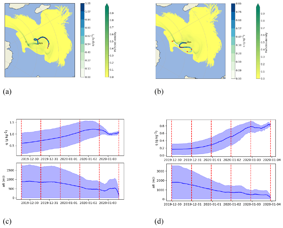
Figure 7 FLEXPART footprints of 5 d back trajectories for the event of 3–4 January. (a) Latitude–longitude projection of the FLEXPART back-trajectory footprints for 3 January 2020 at 13:30. The yellow to green colors at each grid point of these projections represent the density of particles. The white to blue colors indicate the water vapor mixing ratio along the humidity-weighted average back trajectory. Each red point indicates the location of the average back trajectory for each of the 5 d before the date of the considered event. (b) Same as for 3 January 2020 at 22:30. (c) The top shows the evolution of the water vapor mixing ratio of the back trajectories for 3 January 2020 at 13:30; the bottom shows the altitude evolution of the back trajectory for 3 January 2020 at 13:30. (d) Same as panel (c) for 3 January 2020 at 22:30.

The subsidence over the different events can better be studied from the vertical velocity from the ERA5 reanalyses (Figs. 4 and A1). Subsidence (positive vertical velocity) is not systematically associated with negative δ¹⁸O_v excursions: subsidence at either 850 or 500 hPa is observed for only 5 events of 11 (Table 1). In four cases, there is rather an ascending movement of the atmospheric air associated with the rain event. In the other cases, there is no clear vertical movement. However, we note that, when negative δ¹⁸O_v excursions are not concomitant with subsidence, they occur at the end of an ascending movement which is generally followed by subsidence (Figs. A1 and A2).

4.4 Model–data comparison and atmospheric dynamics

With the information gathered above, both subsidence and isotopic depletion associated with rain occurrence and further interaction between droplets and water vapor can explain the negative excursions of δ¹⁸O_v. We note however that the data gathered so far do not permit us to provide a simple and unique explanation. Neither subsidence nor rain systematically occurred for each of the δ¹⁸O_v excursions. Still, the fact that at least ECHAM6-wiso is able to reproduce every negative δ¹⁸O_v excursion (whether they are associated or not with subsidence or rainwater vapor re-equilibration) shows that (1) the patterns of the atmospheric water cycle are correctly reproduced, a validation which can be performed using humidity and precipitation data for some aspects while benefitting from water isotope implementation for the residence time of water; and (2) the isotopic processes are correctly implemented in this model. Such abrupt δ¹⁸O_v events can hence be used as a test bed of the performances of water-isotope-enabled general circulation models.

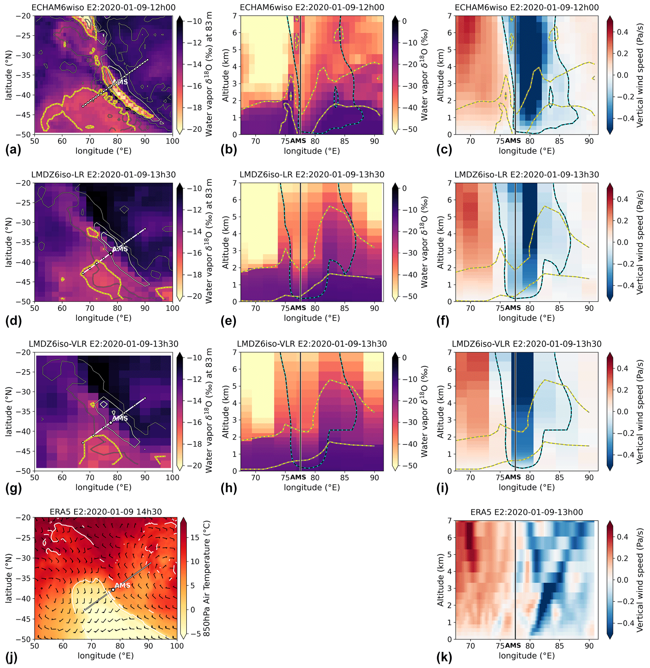
Figure 8 Modeled δ¹⁸O_v and vertical velocity for the event of 9 January 2020. (a) Surface air δ¹⁸O_v (∼ 83 m, latitude vs. longitude), with yellow lines indicating the −15 ‰ contour level and grey lines indicating precipitation contours at 0.5, 10, and 50 mm d⁻¹ (thin, medium, and thick lines, respectively). (b) δ¹⁸O_v plotted on a vertical cross section (altitude vs. longitude) along the transect indicated by the white line in panel (a), with yellow lines indicating δ¹⁸O_v contours at −30 ‰ and −15 ‰, blue lines indicating the contour of −0.05 Pa s⁻¹ vertical velocity (ascendance), and the vertical black line denoting the longitude of Amsterdam Island. (c) Vertical velocity plotted on a vertical cross section as for panel (b) with the same contour lines. Panels (a), (b), and (c) are drawn using outputs of the ECHAM6-wiso model. Panels (d), (e), and (f) are the same as panels (a), (b), and (c) but obtained from the LMDZ-iso model at low resolution (LR). Panels (g), (h), and (i) are the same as panels (a), (b), and (c) but obtained from the LMDZ-iso model at very low resolution (VLR). (j) ERA5 air temperature at 850 hPa, with white lines marking front locations (see Fig. S1). (k) ERA5 vertical velocity plotted on a vertical cross section (altitude vs. longitude) along the transect indicated by the black dotted line in panel (j).

To further explore the δ¹⁸O_v data–model comparison and the associated processes, we compare the performances of the ECHAM6-wiso and LMDZ-iso models over the first months of 2020 in terms of atmospheric dynamics (Figs. 4 and A1). First, and as expected because of the nudging, the two models reproduce rather well the evolution of the vertical velocity of the ERA5 reanalyses, with a stronger ascent for the model predicting the strongest precipitation amount (e.g., LMDZ-iso for 24 January 2020). The event of 3 January is the only one reproduced by both ECHAM6-wiso and the two versions of the LMDZ-iso model: the three simulations show a clear subsidence over the isotopic event and a clear negative δ¹⁸O_v excursion. For the other events, neither LMDZ-iso nor ECHAM6-wiso shows a clear signal of subsidence at 500 or 850 hPa (not shown). However, the horizontal distributions of vertical velocity obtained with ECHAM6-wiso and LMDZ-iso are significantly different (Fig. 8 for the event of 9 January, Figs. S2 and S3 for the other events). While the LMDZ-iso-modeled vertical velocity displays a rather strong homogeneity on the vertical axis, the ECHAM6-wiso-modeled vertical velocity highlights subsidence of air below the ascending column, with the maximum of the negative δ¹⁸O_v anomaly at the surface located just at the limit between ascendance and subsidence (between 75 and 77° E in Fig. 8c). This subsidence of depleted δ¹⁸O_v below the ascending column is responsible for the sharp negative δ¹⁸O_v excursion in the ECHAM6-wiso model. The fact that subsidence of air occurs just below uplifted air, at the limit between ascendance and subsidence (Figs. 8k and S2), permits us to reconcile the GEM data, suggesting subsidence, and the sign of the vertical velocity of the ERA5 reanalyses at Amsterdam Island suggests that many excursions start with ascendance. Since the isotope implementation was done similarly in the two models, the reason why the LMDZ-iso model does not reproduce the water isotopic anomaly is its too coarse resolution, as also supported by the comparison between performances of the LMDZ-iso model at low resolution and very low resolution for the event of 24 January (Table 1 and Fig. 4). As already pointed out by Ryan et al. (2000), a fine resolution is necessary for correctly simulating front dynamics, and we extend this result here to the high-resolution temporal patterns of surface δ¹⁸O_v.

4.5 Synthesis

Figure 9 summarizes the proposed mechanism for negative δ¹⁸O_v excursions as inferred from our data–model comparison when there is a clear rain event. A rain event is associated with a strong ascending column in which δ¹⁸O_v is depleted by progressive precipitation during the ascent and by interaction between rain and water vapor. This ascending column is generally associated with a cold front moving from southwest to northeast (Figs. 8j and S1), with subsidence and δ¹⁸O_v-depleted air at the rear of the front (Figs. 8, S2, and S3).

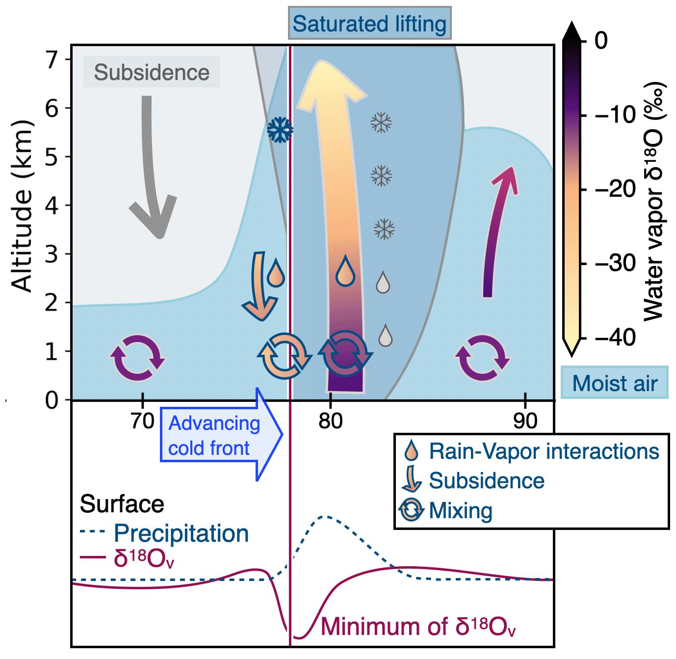
Figure 9 Scheme of the mechanism explaining the sharp negative excursion of δ¹⁸O_v recorded at the surface for cold-front events associated with precipitation. The scheme is based on the profile modeled by ECHAM6-wiso for the event of 9 January 2020 (see Fig. S5 for the other events). The top panel shows the altitude vs. longitude dynamics of air masses with vertical saturated lifting in the center and subsidence at the rear of the lifting. The bottom panel shows the associated evolution of δ¹⁸O_v and precipitation on the same longitude scale as the upper panel.

5 Conclusion

We presented here the first water vapor isotopic record over 2 years on Amsterdam Island. The water vapor isotopic variations follow at first order the variations of the water vapor mixing ratio, as expected for such a marine site. Superimposed on this variability, we have shown 11 periods of a few hours characterized by the occurrence of one or two abrupt negative excursions of δ¹⁸O_v, while the correlation between δ¹⁸O_v and the water vapor mixing ratio does not hold. These negative excursions often occur toward the end of precipitation events. Most of the time they occur during a decrease in the water vapor mixing ratio. Representation of these short events is a challenge for the atmospheric components of Earth system models equipped with water isotopes, and we found that the ECHAM6-wiso model was able to reproduce most of the sharp negative δ¹⁸O_v excursions, while the LMDZ-iso model at low (very low) resolution was only able to reproduce seven (one) of the negative excursions. The good agreement between modeled and measured δ¹⁸O_v when using ECHAM6-wiso validates the physics processes within the ECHAM6-wiso model as well as the implemented physics of water isotopes.

Using previous modeling studies as well as information provided by (1) the confrontation with other data sources (GEM, meteorology) obtained in parallel on this site, (2) back-trajectory analyses, and (3) the outputs of the two models ECHAM6-wiso and LMDZ-iso, we conclude that the most plausible explanations for such events are rain–vapor interactions and subsidence at the rear of a precipitation event. Both can be combined, since rain–vapor interactions can help maintain moist conditions in subsidence regions.

This study highlights the added value of combining different data from a surface atmospheric observatory to understand the dynamics of the atmospheric circulation, e.g., subsidence in the higher atmosphere. These 2-year records are also a good benchmark for model evaluation. We have especially shown that the isotopic composition of water vapor measured at the surface is a powerful tool for testing the vertical dynamics of atmospheric models and the implementation of water isotopes for those that are equipped with them. In our case, we used it to test different horizontal resolutions which influence the representativity of the vertical dynamics and have important implications in the simulation of surface variations of water vapor δ¹⁸O_v. Our study highlights the importance of having high-resolution models (e.g., mesoscale models) equipped with isotopes to further study such abrupt isotopic events.

Appendix A

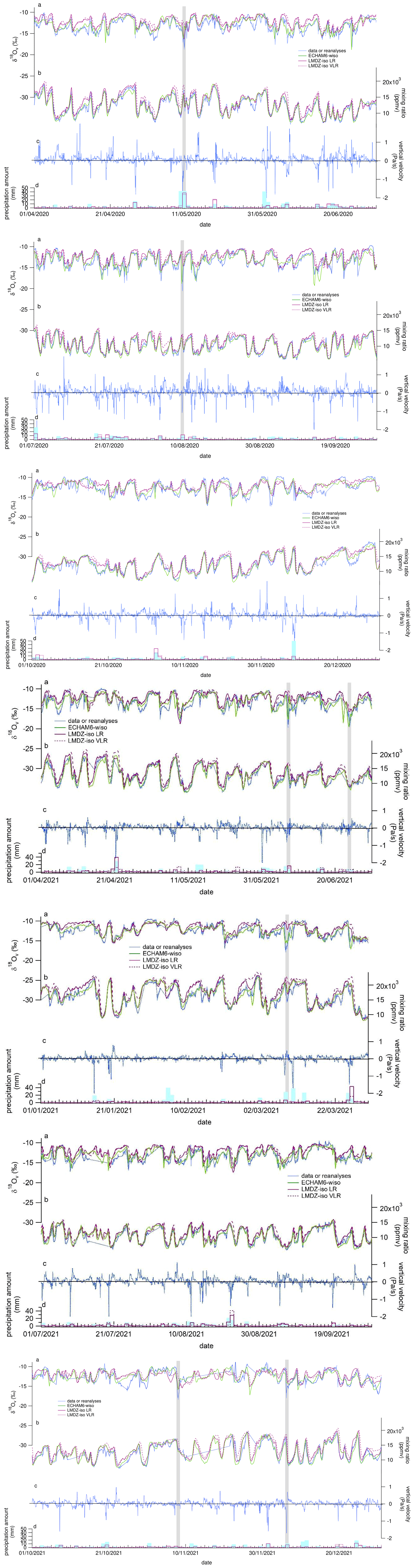
Figure A1 Model–measurement comparison (April 2020–December 2021). (a) δ¹⁸O_v (light blue for data on an hourly average, dark blue for data resampled at a 6 h resolution). (b) Water vapor mixing ratio from our dataset. (c) Vertical velocity. (d) Precipitation amount. The grey shadings highlight the negative δ¹⁸O_v excursions.

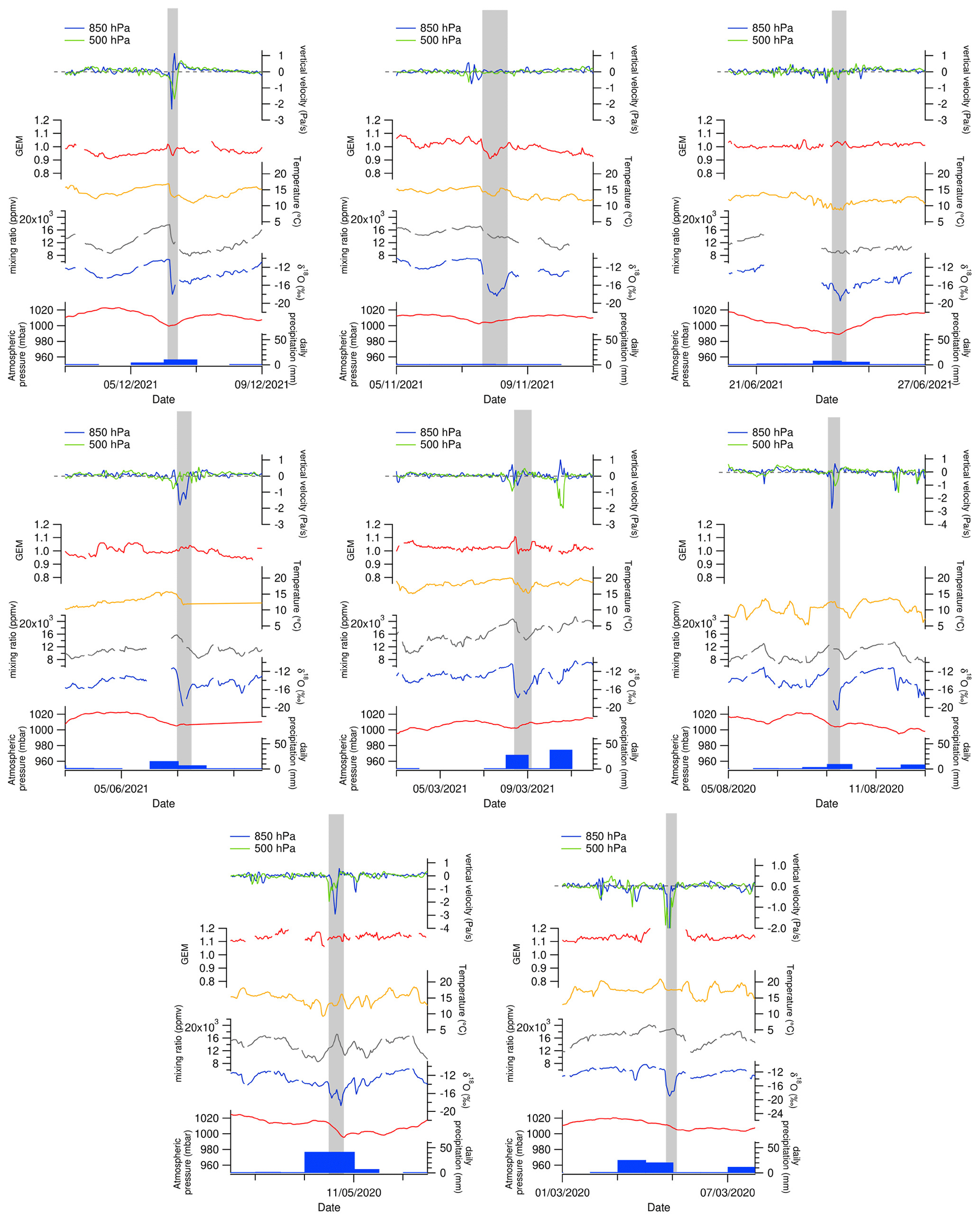
Figure A2 Evolution of GEM, δ¹⁸O_v, water vapor mixing ratio, meteorological parameters (surface temperature, surface atmospheric pressure, daily precipitation) measured by the Météo-France weather station, and vertical velocity from the ERA5 reanalyses at 500 and 850 hPa over the isotopic excursions between March 2020 and December 2021.

Figure A3 FLEXPART footprints of 5 d back trajectories for the event of 9 January 2020. (a) Latitude–longitude projection of the FLEXPART back-trajectory footprint for 9 January 2020 at 07:30. The yellow to green colors at each grid point of these projections represent the density of the particles. The white to blue colors indicate the water vapor mixing ratio on the humidity-weighted average back trajectory. Each red point indicates the location of the average back trajectory for each of the 5 d before the date of the considered event. (b) Same as for 9 January 2020 at 13:30. (c) The top shows the evolution of the water vapor mixing ratio of the back trajectories for 9 January 2020 at 07:30; the bottom shows the altitude evolution of the back trajectory for 9 January 2020 at 07:30. (d) Same as panel (c) for 9 January 2020 at 13:30.

Figure A4 FLEXPART footprints of 5 d back trajectories for the event of 21 January 2020. (a) Latitude–longitude projection of the FLEXPART back-trajectory footprint for 21 January 2020 at 07:30. The yellow to green colors at each grid point of these projections represent the density of the particles. The white to blue colors indicate the water vapor mixing ratio on the humidity-weighted average back trajectory. Each red point indicates the location of the average back trajectory for all 5 d before the date of the considered event. (b) Same as for 21 January 2020 at 13:00. (c) The top shows the evolution of the water vapor mixing ratio of the back trajectories for 21 January 2020 at 07:30; the bottom shows the altitude evolution of the back trajectory for 21 January 2020 at 07:30. (d) Same as panel (c) for 21 January 2020 at 13:00.